Embed Size (px)
Citation preview

HAL Id: hal-00768234https://hal.inria.fr/hal-00768234v3
Submitted on 12 Feb 2013
HAL is a multi-disciplinary open accessarchive for the deposit and dissemination of sci-entific research documents, whether they are pub-lished or not. The documents may come fromteaching and research institutions in France orabroad, or from public or private research centers.
L’archive ouverte pluridisciplinaire HAL, estdestinée au dépôt et à la diffusion de documentsscientifiques de niveau recherche, publiés ou non,émanant des établissements d’enseignement et derecherche français ou étrangers, des laboratoirespublics ou privés.
Modeling and simulation of a grand piano.Juliette Chabassier, Antoine Chaigne, Patrick Joly
To cite this version:Juliette Chabassier, Antoine Chaigne, Patrick Joly. Modeling and simulation of a grand piano..[Research Report] RR-8181, INRIA. 2012, pp.29. hal-00768234v3
ISS
N0
24
9-6
39
9IS
RN
INR
IA/R
R--
81
81
--F
R+
EN
G
RESEARCH
REPORT
N° 8181December 2012
Project-Teams Poems and Magique 3d
Modeling and simulation
of a grand piano.
Juliette Chabassier, Antoine Chaigne, Patrick Joly


RESEARCH CENTRE
BORDEAUX – SUD-OUEST
200 Avenue de la Vieille Tour,
33405 Talence Cedex
Modeling and simulation of a grand piano.
Juliette Chabassier∗†, Antoine Chaigne‡, Patrick Joly †
Project-Teams Poems and Magique 3d
Research Report n° 8181 — December 2012 — 35 pages
Abstract: A time-domain global modeling of a grand piano is presented. The string modelincludes internal losses, stiffness and geometrical nonlinearity. The hammer-string interaction isgoverned by a nonlinear dissipative compression force. The soundboard is modeled as a dissipativebidimensional orthotropic Reissner-Mindlin plate where the presence of ribs and bridges is treatedas local heterogeneities. The coupling between strings and soundboard at the bridge allows thetransmission of both transverse and longitudinal waves to the soundboard. The soundboard iscoupled to the acoustic field, whereas all other parts of the structure are supposed to be perfectlyrigid. The acoustic field is bounded artificially using perfectly matched layers (PML). The discreteform of the equations is based on original energy preserving schemes. Artificial decoupling isachieved, through the use of Schur complements and Lagrange multipliers, so that each variableof the problem can be updated separately at each time step. The capability of the model ishighlighted by series of simulations in the low, medium and high register, and through comparisonswith waveforms recorded on a Steinway D piano. Its ability to account for phantom partials andprecursors, consecutive to string nonlinearity and inharmonicity, is particularly emphasized.
Key-words: piano, modeling, time-domain, simulation, nonlinear strings, string-soundboardcoupling, radiation
∗ Magique 3d team† Poems team‡ UME Ensta
Modelisation et simulation numerique d’un piano a queue.
Resume : Un modele de piano a queue en domaine temporel est presente. Le modele decorde decrit les pertes internes, la raideur et la non linearite geometrique. L’interaction marteau-corde est dictee par une force non lineaire dissipative de compression. La table d’harmonie estmodelisee comme une plaque bidimensionnelle de Reissner-Mindlin dissipative, les raidisseurs et lechevalet etant traites comme des heterogeneites locales. Le couplage entre les cordes et la tableau chevalet permet la transmission des ondes transversales et longitudinales la table. La table estcouplee au champ acoustique, tandis que toutes les autres parties de la structure sont supposeesrigides. Le champ acoustique est tronque artificiellement l’aide de PML. La formulation discretedes equations se base sur l’utilisation de schemas numeriques preservant l’energie. Le potentiel dumodele est demontre via une serie de simulations en bas, medium et haut registre, ainsi que viades comparaisons avec des formes d’ondes enregistrees sur un piano queue Steinway-D. Sa capaciterendre compte des partiels fantmes et du precurseur, consequence de la non linearite des cordesconjointe leur inharmonicite, est particulierement mise en valeur.
Mots-cles : piano, modelisation, domaine temporel, simulation, cordes non lineaires, couplagecordes - table d’harmonie, rayonnement

Modeling a piano. 3
1 Introduction
In this paper, an extensive and global model of a piano is presented. Its aim is to reproduce themain vibratory and acoustic phenomena involved in the generation of a piano sound from the initialblow of the hammer against the strings to the radiation from soundboard to the air. Comparedto previous studies, the prime originality of the work is due to the string model which takes bothgeometrical nonlinear effects and stiffness into account. Other significant improvements are due tothe combined modeling of the three main couplings between the constitutive parts of the instrument:hammer-string, string-soundboard and soundboard-air coupling.
Although a vast literature exists on the piano and its subsystems (strings, hammer, soundboard,radiated field), there are only a few examples of a complete computational model of the instrument.One noticeable exception is the work by Giordano and Jiang [1] describing the modeling of a linearstring coupled to soundboard and air using finite differences. Compared to this reference, our workis based on a more accurate description of the piano physics, and also pays more attention to theproperties of the numerical schemes used for solving the complex system of coupled equations. Thestrategy used here for the piano is similar to the one developed previously by two of the authors forthe guitar [2] and the timpani [3]. The physical model is composed of a set of equations governingthe hammer-string contact and the wave propagation in strings, soundboard and air, in the timedomain. The input parameters of the equations are linked to the geometry and material propertiesof the propagation media. The equations are then discretized in time and space, in order to allowthe numerical resolution of the complete system. Original numerical schemes are developed in orderto ensure stability, sufficient accuracy and the conservation of energy. In this respect, this strategyhas a direct continuity with the work by Bilbao [4].
The numerical dispersion of the schemes is maintained sufficiently small so that the differencebetween real and simulated frequencies are comparable to the just noticeable differences of thehuman ear in the audible range (around 1 %). The validity of the numerical model is assessed bycareful analysis, in time and frequency, of the most significant variables of the problem: hammerforce, string, bridge and soundboard displacements (resp. velocities or accelerations), sound pres-sure. In a first step, using typical values of parameters found in the literature, the numerical resultsare expected to reproduce the main features of piano sounds, at least qualitatively. In a secondstep, the input parameters are the results of measurements on real pianos, and a more thoroughcomparison is made between real and simulated tones.
One motivation at the origin of this study was to reproduce the effects of the geometrical nonlin-earity of piano strings both in time (precursors[5], transverse-longitudinal coupling) and frequencydomain (phantom partials[6]). The purpose of the simulations is to get a better understandingof these phenomena: the aim is to exhibit quantitative links between some control parameters(initial hammer velocity, string tension,...) and observed waveforms and spectra. Experimentalobservations of string and soundboard spectra recorded on real pianos suggest, in addition, thatthe string-soundboard coupling plays a crucial role in the transmission of longitudinal string com-ponents [7], and thus attempting to reproduce and understand these effects is another challenge.
In pianos, it is well-known that the initial transients are perceptually highly significant. Onemajor attribute of spectral content during the attack is due to the presence of soundboard modesexcited by the string force at the bridge. The low-frequency modes, in particular, have low damping:they are well separated and clearly recognizable on the spectra [8]. An accurate model of string-soundboard coupling has the capability of accounting for such effects. Soundboard modeling alsoallows to explore the effects of bridge and ribs distribution on the produced sound.
RR n° 8181

Modeling a piano. 4
Finally, air-soundboard coupling is a necessary step for simulating sound pressure. Becauseof the wideband modeling, the computation of a 3-D pressure field is highly demanding. Highperformance parallel computing was necessary here. However, the results are very valuable, sinceone can make direct auditory comparisons with real piano sounds. Simulation of a 3-D field alsoyields information on directivity and sound power.
The physical model of the piano used in this work is presented in Section 2. Emphasis isput on what we believe to be the most innovative parts of the model: the nonlinear stiff stringand its coupling with an heterogeneous orthotropic soundboard via the bridge. Hammer-stringinteraction and air-soundboard coupling are also described. In Section 3, the general method usedfor putting the model into a discrete form is explained. The properties of the main numericalschemes retained for each constitutive part of the instrument and the coupling conditions are givenwithout demonstrations, with explicit references to other papers published by the authors, that aremore oriented on the mathematical and numerical aspects of the model.
The validity of the model is evaluated in Section 4 through analysis of a selection of simulatedpiano notes in the low, medium and treble register, respectively. The motion of the main elements(piano hammer, strings, bridge, soundboard, air) are analyzed alternatively in time, space, and/orfrequency domain. Because of the important effort put on the nonlinear string, the capability ofthe model to reproduce amplitude-dependent phenomena is emphasized. Comparisons are alsomade with measurements performed on a Steinway grand piano (D model). In these series ofexperiments, the motion of hammer, string, bridge and soundboard, and the sound pressure wererecorded simultaneously. This shed useful light on the transmission and transformation of thesignals from hammer to sound and, through comparisons, on the ability of the model to accountfor the coupling between the constitutive parts of the piano.
2 Presentation of the model
During the development of the model, particular attention was paid to the following guidelines:
• The prime function of the piano is to generate sounds. However, its conception is not onlygoverned by dynamical and acoustical laws, but also by purely static and mechanical consid-erations, as it is the case, for example, for the design of frame, rim and feet. In addition,from the point of view of the player, the piano must fulfill a number of playability rules. Ourpurpose is not to mimic piece by piece the construction of a real instrument, but rather todescribe the major phenomena that are at the origin of piano tones. This is achieved hereby considering a set of equations governing the nonlinear hammer-string contact, the wavepropagation in strings, the vibrations of the heterogeneous orthotropic soundboard radiatingin air, and the reciprocal coupling between strings and soundboard at the bridge.
• Several simplifying assumptions were made in the model. The hammer is supposed to beperfectly aligned with the strings. The agraffe is assumed to be rigidly fixed with a simplysupported end condition for the strings. Both the string-soundboard and soundboard-aircouplings are supposed to be lossless. The soundboard is considered as simply supportedalong its edge, and the “listening” room is anechoic with no obstacle except the piano itself.Finally, the action of the mechanism prior to the shock of the hammer against the strings isignored. In other words, the tone starts when the hammer hits the strings with an imposedvelocity.
RR n° 8181

Modeling a piano. 5
• Most of the physical parameters of hammers, strings and soundboards included in the modelare obtained from standard string scaling and geometrical data from piano, strings and sound-boards manufacturers. When necessary, these data were complemented by results of our ownmeasurements on various instruments. However, some difficulties arose for the physical de-scription of damping models in hammers, strings and soundboards since the underlying phys-ical mechanisms are often very complex, and because an accurate analytical description ofthese phenomena are not available in the present state-of-the-art. Thus, it was decided to usehere approximate models based on experimental data, as it is commonly done in other fieldsof structural dynamics [9].
• As shown in Section 3, the numerical formulation of the model is based on a discrete for-mulation of the global energy of the system, which ensures stability. This requires that thecontinuous energy of the problem is decaying with time. The global model of the piano isthus written according to this condition.
In what follows, an energy decaying model is developed for each constitutive part of the instrument,successively. Finally, a global piano model is proposed.
2.1 Strings
The selected string model accounts for large deformations, inducing geometrical nonlinearities,and intrinsic stiffness. These are two essential physical phenomena in piano strings [10, 11]. Thegoverning equations correspond to those of a Timoshenko beam under axial tension. Modeling thestiffness with a Timoshenko model, rather than with an Euler-Bernoulli model as in a previousstudy by Chaigne and Askenfelt [12], is motivated by both physical and numerical reasons. Asshown in Fig. 13 of Section 4, the physical dispersion predicted by the Timoshenko model shows agood agreement with experimental data in a wider frequency range than the Euler-Bernoulli model.It also yields an asymptotic value for the transverse wave velocity as the frequency increases, incontrast with the Euler-Bernoulli model. This latter property is not only more satisfying fromthe point of view of the physics, but it is also more tractable in the simulations. The geometricalnonlinearities are described using a standard model[13].
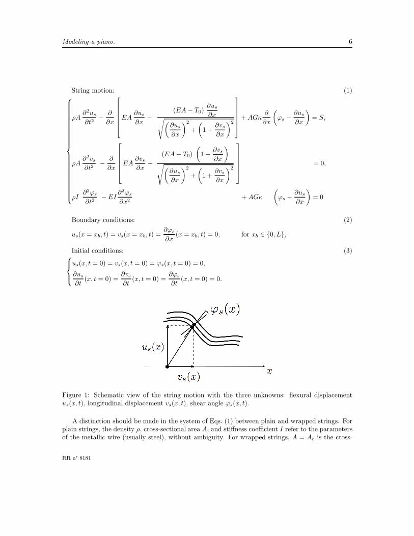
Let us call ρ the density of the string, A the area of its cross-section, T0 its tension at rest, Eits Young’s modulus, I its stiffness inertia coefficient, G its shear coefficient, and κ the nondimen-sional Timoshenko parameter. We denote us(x, t) the transverse vertical displacement, vs(x, t) thelongitudinal displacement, and ϕs(x, t) the angle of the cross-sections with the plane normal to thestring (see Fig. 1). The space variable is x ∈ [0, L], where L is the length of the string at rest. Forthe end conditions, we assume zero displacement (in both transverse and longitudinal directions)and zero moment. These conditions are motivated by usual observations at the agraffe (x = 0)[14], and will be revisited later at point x = L when considering the coupling with the soundboard.Finally, the string is considered at rest at the origin of time. We get the following system (1), whereS is a source term. As shown in the next paragraph, this term is supposed to account for the actionof the hammer against the strings. The model is written:
RR n° 8181
Modeling a piano. 6
String motion: (1)
ρA∂2us
∂t2−
∂
∂x
EA∂us
∂x−
(EA− T0)∂us
∂x√
(
∂us
∂x
)2
+
(
1 +∂vs∂x
)2
+AGκ∂
∂x
(
ϕs −∂us
∂x
)
= S,
ρA∂2vs∂t2
−∂
∂x
EA∂vs∂x
−
(EA− T0)
(
1 +∂vs∂x
)
√
(
∂us
∂x
)2
+
(
1 +∂vs∂x
)2
+AGκ∂
∂x
(
ϕs −∂us
∂x
)
= 0,
ρI∂2ϕs
∂t2− EI
∂2ϕs
∂x2+AGκ
∂
∂x
(
ϕs −∂us
∂x
)
= 0
Boundary conditions: (2)
us(x = xb, t) = vs(x = xb, t) =∂ϕs
∂x(x = xb, t) = 0, for xb ∈ 0, L,
Initial conditions: (3)
us(x, t = 0) = vs(x, t = 0) = ϕs(x, t = 0) = 0,
∂us
∂t(x, t = 0) =
∂vs∂t
(x, t = 0) =∂ϕs
∂t(x, t = 0) = 0.
Figure 1: Schematic view of the string motion with the three unknowns: flexural displacementus(x, t), longitudinal displacement vs(x, t), shear angle ϕs(x, t).
A distinction should be made in the system of Eqs. (1) between plain and wrapped strings. Forplain strings, the density ρ, cross-sectional area A, and stiffness coefficient I refer to the parametersof the metallic wire (usually steel), without ambiguity. For wrapped strings, A = Ac is the cross-
RR n° 8181

Modeling a piano. 7
sectional area of the core, I = Ic is the stiffness coefficient of the core, whereas ρ = ρcF where ρcis the density of the core, and F is a wrapping factor (see Conklin[14]) defined by the expression:
F = 1 +ρwAw
ρcAc
, (4)
where Aw is the cross-sectional area of the wrapping with density ρw (usually copper). In bothcases, the other parameters E, T0, G, κ refer to the material of the wire (resp. core). In short, thewrapping affects the inertial forces only.The eigenfrequencies of the linearized version of system (1) associated with boundary conditions(2) can be computed analytically (see, for example[17]), which yield three different series. Thefollowing expressions hold for partial’s rank ℓ ≥ 1. The flexural eigenfrequencies are given by:
f transℓ = ℓf trans
0
(
1 + ǫ ℓ2)
+O(ℓ5), where f trans0 =
1
2L
√
T0
ρA, ǫ =
π2
2L2
EI
T0
[
1−T0
EA
]
. (5)
The shear eigenfrequencies satisfy:
f shearℓ = f shear
0
(
1 + η ℓ2)
+O(ℓ4), where f shear0 =
1
2π
√
AGκ
ρI, η =
π2
2L2
EI + IGκ
AGκ. (6)
These shear frequencies, which are situated well above the audio range, are not perceived by thehuman ear. Finally, the longitudinal eigenfrequencies read
f longiℓ = ℓf longi
0 , where f longi0 =
1
2L
√
E
ρ. (7)
Eq. (5) shows that the model accounts for inharmonicity. The inharmonicity coefficient ǫ is close to,but slightly different from, the usual coefficient obtained with the Euler-Bernoulli model[18]. The
speed of waves associated to equations (5) and (7) are the transverse speed ctrans =√
T0/ρA and
the longitudinal speed clongi =√
E/ρ. For the string C2, for example, we obtain ctrans = 209 m·s−1
and clongi = 2914 m·s−1. Since both types of waves are present on the string (because of nonlineartransverse to longitudinal coupling) near the hammer contact point, the speed ratio explains whythe longitudinal waves arrive first at the bridge, inducing a precursor.
With the objective to simulate realistic tones, it is essential to account for the observed frequency-dependent damping on strings. Damping phenomena in structures in general, and in strings inparticular, are hard to apprehend, for many reasons (lack of available measurements, uneasy sep-aration of the mechanisms, difficulty in modeling microscale phenomena such as dislocations, inthe equation of motion,. . . ). Therefore, following the strategy used in previous studies, we use asimple model that globally and approximately accounts for the damping effect, without pretendingto model the underlying physics in details [19]. In practice, viscoelastic terms are added under theform:
2 ρARu
∂us
∂t− 2T0 ηu
∂3us
∂t ∂x2(8)
where Ru and ηu are empirical damping coefficients to be determined from measured sounds foreach string, through comparisons between simulated and measured spectrograms. The resulting
RR n° 8181

Modeling a piano. 8
damping law in the frequency domain is the sum of a constant term 2 ρARu and a quadratic term2T0 ηu f
2ℓ . Similar damping terms have to be added for shear and longitudinal motions in order to
avoid unpleasant endless frequencies in the simulated tones.
2 ρARv
∂vs∂t
− 2EAηv∂3vs∂t ∂x2
, 2 ρI Rϕ
∂ϕs
∂t− 2EI ηϕ
∂3ϕs
∂t ∂x2. (9)
Again, the order of magnitude for (Rv, Rϕ) and (ηv, ηϕ) are determined from experiments and/ortrial-and-error procedures, considering the absence of any other reliable method.
When the system is subjected to a source term S(x, t) in the transverse direction, it is possibleto show the following energy identity [20]:
dEsdt
≤
∫ L
0
S∂us
∂tdx where Es(t) = Es,kin(t) + Es,pot(t) (10)
Es,kin(t) =ρA
2
∫ L
0
(
∂us
∂t
)2
dx+ρA
2
∫ L
0
(
∂vs∂t
)2
dx+ρI
2
∫ L
0
(
∂ϕs
∂t
)2
dx
Es,pot(t) =T0
2
∫ L
0
(
∂us
∂x
)2
dx+EA
2
∫ L
0
(
∂vs∂x
)2
dx
+EI
2
∫ L
0
(
∂ϕs
∂x
)2
dx+AGκ
2
∫ L
0
(
∂us
∂x− ϕs
)2
dx
+ (EA− T0)
∫ L
0
1
2
(
∂us
∂x
)2
+
(
1 +∂vs∂x
)
−
√
(
∂us
∂x
)2
+
(
1 +∂vs∂x
)2
dx
This quantity is always positive in practice since, for real piano strings, we have EA > T0. Advan-tage of this property will be taken in Section 3 to derive stable numerical schemes for solving thenonlinear system of equations.
2.2 Hammer
We now turn to the interaction between the hammer and the strings. Depending on the note,the hammer strikes one, two or three strings. The components of the motion of the ith string’sof a given note’s set are written (us,i, vs,i, ϕs,i). Since the strings belonging to the same note areslightly detuned[21], each string has a different tension at rest T0,i in system (1). The hammer’scenter of gravity is supposed to be moving along a straight line orthogonal to the strings at rest.Its displacement on this line is represented by ξ(t). The interaction force between the hammer andthe ith-string of a note is distributed on a small portion of the string, through a spreading function
δH (represented in Fig. 2) localized around the impact point x0, with
∫ L
0
δH(x) dx = 1.
As a consequence, we denote 〈us,i〉 the weighted average of the transverse displacement of thestring:
〈us,i〉(t) =
∫ L
0
us,i(x, t) δH(x) dx. (11)
RR n° 8181

Modeling a piano. 9
Figure 2: Spreading function δH(x) used to model the hammer string contact. The width of thecontact zone is about 2 cm.
The interaction force depends on the distance d(t) between the hammer and the string: if d(t) > ξ,there is no contact and the force is zero. If d(t) ≤ ξ, the force is a function of the distance.According to previous studies, we define the function:
Φ(d) =[
(
ξ − d)+
]p
(12)
where (·)+ means “positive part of”, and where p is a real positive nonlinear exponent. In practice,this coefficient varies between 1.5 and 3.5 [22, 23, 12]. In order to account further for the observedhysteretic behavior of the felt[22], a dissipative term is added in the expression of the force. Insummary, the parameters characterizing the mechanical behavior of the hammer are its equivalentmass MH, its stiffness coefficient KH
i and its dissipation coefficient RH
i . The index i here indicatesthat the model can eventually account for the fact that the interaction with the hammer might notbe uniform for each string of a note. The interacting force between the hammer and the ith-stringfinally reads
FH
i (t) = KH
i Φ(
〈us,i〉(t)− ξ(t))
+RH
i
d
dtΦ(
〈us,i〉(t)− ξ(t))
. (13)
The hammer is submitted to the sum of these forces. Conversely, the right hand side S(x, t) of thestrings system (1) is replaced with FH
i (t) δH(x).We consider an initial position −ξ0 and an initial velocity vH0 for the hammer, while the strings
are considered at rest at the origin of time. Defining further Ψ(d) =
∫ +∞
d
Φ(s) ds, one can show
(see Chabassier et al. [20]) that any regular solution to the resulting hammer – strings systemsatisfies the following energy decay:
dEs,hdt
≤ 0, with Es,h(t) =∑
i
[
Es,i(t) +KH
i Ψ(
〈us,i〉(t)− ξ(t))
]
+MH
2
(
dξ
dt(t)
)2
≥ 0 (14)
where Es,i(t) is the energy defined in Eq. (10) for the ith string.
2.3 Soundboard
The only vibrating element of the piano case considered in the model is the soundboard, all otherparts (rim, keybed, lid, iron frame. . . ) being assumed to be perfectly rigid. In view of the small“thickness over other dimensions” ratio of the piano soundboard, a bidimensional Reissner-Mindlinplate model is considered. This model is the bidimensional equivalent to the linear Timoshenkomodel. It has been preferred here to the Kirchhoff-Love model, because its yields a better estimate
RR n° 8181

Modeling a piano. 10
for the soundboard motion, in the complete audio range. It also has better mathematical properties[20]. The variables of the motion are the vertical transverse displacement up(x, y, t) at a currentpoint of coordinates (x, y) of the bidimensional plate ω, and two shear angles θx,p(x, y, t) andθy,p(x, y, t). These last two variables account for the deviation of the straight segments of the platefrom the normal to the medium surface, in the (ex, ey)-referential plane (see Fig. 3). The vectorθp(x, y, t) groups these two angles. The bridge and ribs are considered as heterogeneities of thesoundboard, and the orientation of the orthotropy axes can be space dependent. As a consequence,the physical coefficients representing the density ρp, the thickness δ, the Young’s moduli in thetwo main directions of orthotropy Ex and Ey , the shear moduli in the three main directions oforthotropy Gxy, Gxz and Gyz, the Poisson’s ratios νxy and νyx, and the shear coefficient κx and κy
are functions of space.Modeling the thickness as a space dependent variable makes it possible to simulate a diaphrag-
matic soundboard [24] (the thickness varies between 6 and 9 mm in the soundboard, between 9and 35 mm on the ribs, between 29 and 69 mm on the bridge, and between 29 and 95 mm on thecrossing areas of ribs and bridge). The soundboard is assumed to be simply supported[25] on itsedge ∂ω. Finally, a source term is imposed in the transverse vertical direction. The function of thisterm is to account for both the string’s tension at the bridge (see Section 2.4) and the air pressurejump (see Section 2.5).
Figure 3: Schematic view of the four different zones of the soundboard in the referential plane. Theorthotropy axis of the soundboard makes an angle of −40 degrees with the horizontal axis (see thestripes).
For simplicity, the rotation of the orthotropy axes in the soundboard is ignored in the presen-tation of the equations, although this flexibility is possible in the model. The Reissner-Mindlinsystem that governs the motion of transverse displacement and shear angles is written for (x, y)
RR n° 8181

Modeling a piano. 11
Table 1: Parameters used for the wooden soundboard: Spruce for the table and the ribs, Beech forthe bridge.
ρp Ex Ey Gxy Gxz Gyz νxy(kg·m−3) (GPa) (GPa) (GPa) (GPa) (GPa)
Spruce 380 11.0 0.650 0.66 1.2 0.042 0.26Beech 750 13.7 2.24 1.61 1.06 0.46 0.3
belonging to the 2D domain ω:
ρpδ3
12
∂2θp∂t2
−Div
(
δ3
12C ε(θp)
)
+ δ κ2 ·G · (∇up + θp) = 0 (15a)
ρp δ∂2up
∂t2− div
(
δ κ2 ·G · (∇up + θp))
= f (15b)
up = Cε(θp)n = 0 on ∂ω (15c)
with C ε =
Ex
1− νxyνyx−
Eyνxy1− νxyνyx
0
−Exνyx
1− νxyνyx
Ey
1− νxyνyx0
0 0 2Gxy
εxxεyyεxy
where the tensor ε is symmetric,
G =
(
Gxz
Gyz
)
, κ2 =
(
κ2x
κ2y
)
(16)
Here, Div is the divergence operator for tensors: Div(τ) = ∂jτi,j , ε is the linearized strain ten-sor, div is the divergence operator for R
2 vectors and ∇ is the gradient operator. Table 1 givesthe parameters used for the soundboard wood (Spruce for the table and the ribs, Beech for thebridge). A prestress term can be added to this model, if necessary, accounting for the static actionof the strings on the curved soundboard. Since this action contributes to reduce the initial crownof the soundboard in such a way that it becomes almost flat in normal use, the curvature and theprestress of the soundboard are ignored here.
With regard to the modeling of damping in the soundboard material, a modal approach hasbeen adopted where the modal damping can be adjusted, mode by mode. This method is justifiedas long as the damping factor is small compared to the eigenfrequency, and is of current use instructural dynamics [26]. The modal amplitudes Xn(t) of the nth mode associated to the frequencyfn are then solution of the second-order uncoupled damped oscillators equations:
d2Xn
dt2+ α(fn)
dXn
dt+ (2πfn)
2Xn = Fn (17)
where α is a positive damping function matching experimental data[27], and Fn is the modal con-tribution of the transversal source term f .
RR n° 8181

Modeling a piano. 12
For any positive damping law it is possible to show the following energy identity:
dEpdt
≤
∫ ∫
ω
f∂up
∂tdx dy where Ep(t) = Ep,kin(t) + Ep,pot(t) (18)
Ep,kin(t) =
∫ ∫
ω
ρp δ
(
∂up
∂t
)2
dx dy +
∫ ∫
ω
ρpδ3
12
∣
∣
∣
∣
∂θp∂t
∣
∣
∣
∣
2
dx dy
Ep,pot(t) =
∫ ∫
ω
δ3
12C ε(θp) : ε(θp) dx dy +
∫ ∫
ω
δ κ2 ·G |∇up + θp|2dx dy
Thus, like for the strings-hammer system, we can conclude that the energy of the soundboard decayswith time, after extinction of the source.
2.4 Strings-soundboard coupling at the bridge
The main purpose of the bridge is to transmit the vibrations from the strings to the soundboard.Conversely, the motion of the soundboard drives the string at the bridge. As highlighted by thespectral content of the precursor signal[28], it is essential to model the transmission of both trans-verse and longitudinal waves of the string to the other parts of the structure. The literature isnot very broad concerning this part of the instrument, with a few exceptions [7, 29]. Also fewexperimental data are available, and the wave transmission phenomena occurring at the bridge arestill not clearly understood. For these reasons, we decided to describe a plausible, though not fullyproved, way for transforming the string longitudinal component into a bridge transverse motion.The method is based on the observation that the strings form a slight angle α with the horizontalplane due to both bridge height and soundboard curvature (see Fig. 4-(a)). We also assume that thebridge moves in the vertical direction only. This, again, seems to be a reasonable assumption sincethe static tension of the complete set of strings prevents the bridge to have a significant motion inthe direction of the strings. At this point, we are aware of the fact that some authors were ableto identify and measure such a motion [7], but we must admit that we were no able to exhibitsimilar features in our measurements. It would be probably also necessary in the future to revisitthe assumption of ignoring the horizontal bridge motion perpendicular to the strings, that mightinduce an horizontal component to the string motion.
When the hammer strikes the strings, it gives rise to a transversal wave which, in turn, inducesa longitudinal wave, because of nonlinear geometrical coupling. The longitudinal wave travels 10 to20 times faster than the transverse one, and thus it comes first at the bridge (see Section 2). Theresulting variation of tension is oriented in the direction of the string at rest. Because of the angleformed by the string with the horizontal plane, this induces a vertical component of the longitudinalforce at the bridge, in addition to the transverse force. In our numerical model, the total bridgeforce is distributed in space in the soundboard by means of a rapidly decreasing regular functionχω centered on the point where the string is attached on the soundboard (see Fig. 4-(b)). Theassociated kinematic boundary conditions are the continuity of string and soundboard velocities inthe vertical direction ν, and the nullity of the velocity in the horizontal direction τ at this point(see Fig. 4(a)). These conditions are written formally:
∂us,i
∂t(x = L)
∂vs,i∂t
(x = L)
· ν =
∫
ω
∂up
∂tχω,
∂us,i
∂t(x = L)
∂vs,i∂t
(x = L)
· τ = 0. (19)
RR n° 8181

Modeling a piano. 13
Figure 4: (a) Schematic view of strings-soundboard coupling at the bridge. The soundboard is flatbecause of the static action of the strings. The bridge is supposed to move in the vertical directionν only. The string forms a small angle α with the horizontal plane containing the vector τ . (b) Thespot indicates the spreading function χω for note C2, centered on the point where the string passesover the bridge.
In addition, the source term in the system of Eqs. (15)-(a) to (15)-(c) is given by f = −Fb(t)χω(x, y),where Fb(t) is the bridge force associated to the cinematic conditions written in Eq. (19). Ignoringthe damping terms, and considering only one string for simplicity, this force is written:
Fb(t) = cos(α)
[
EA∂xus +AGκ(
∂xus − ϕs
)
− (EA− T0)∂xus
√
(∂xus)2 + (1 + ∂xvs)2
]
(x = L, t)
+ sin(α)
[
EA∂xvs + (EA− T0)(
1−1 + ∂xvs
√
(∂xus)2 + (1 + ∂xvs)2)
]
(x = L, t) (20)
If the magnitude of the transverse motion remains small enough, it becomes justified under someconditions to derive approximate string models using an asymptotic approach [30]. Such modelswere used in the past by different authors for analytical[31] or numerical[4] purposes. In our case, wewill not use this approximate system for the modeling of the piano, and the mathematical reasonsfor this choice were given explicitely in a previous paper [32]. However, interesting properties canbe derived from the approximate expression of the bridge force:
Fb(t) ≈ cos(α)[
T0 ∂xus +AGκ(
∂xus − ϕc
)
+(EA− T0)∂xus ∂xvs + (EA− T0)(∂xus)
3
2
]
(x = L, t)
+ sin(α)
[
EA∂xvs + (EA− T0)(∂xus)
2
2
]
(x = L, t). (21)
From Eq. (21), it can be derived that the quadratic and cubic terms in us generate double andtriple combinations of the transverse eigenfrequencies[31]. Combination of longitudinal and trans-verse eigenfrequencies can also exist potentially, through the product usvs. All these combinationscorrespond to the so-called “phantom” partials.
RR n° 8181

Modeling a piano. 14
2.5 Sound propagation and structural acoustics
We are now interested in the propagation of piano sounds in free space. The rim (occupying thespace Ωr) is considered to be a rigid obstacle (see Fig. 5). The acoustic velocity V a and theacoustic pressure P are solutions of the linearized Euler equations with velocity ca = 340 m/s,density ρa = 1.29 kg/m3 and adiabatic compressibility coefficient µa = 1/(ρac
2a), in the unbounded
domain Ω = R3 \ ω ∪ Ωr which excludes the rim and the plate:
ρa∂V a
∂t+∇P = 0
µa
∂P
∂t+Div V a = 0
in Ω (22)
Viscothermal losses in the air are ignored in the acoustic model. The normal component of theacoustic velocity vanishes on the rim:
V a · nr = 0 on Ωr (23)
Figure 5: Geometrical configuration of the piano. (Color online)
The coupling between the 3D sound field in Ω and the vibrating soundboard in ω obeys to thecondition of continuity of the velocity normal components:
V a · ez =∂up
∂ton ω (24)
where ez completes the referential (ex, ey) introduced for the describing the motion of the sound-
board in ω ⊂ R2 (see Fig. 5). Finally, the soundboard force f is the pressure jump:
[P ]ω = P |ω− − P |ω+ (25)
RR n° 8181

Modeling a piano. 15
where ω+ and ω− stand for the both sides the plate. Again, the vibroacoustic system satisfies thefollowing energy decay:
dEp,adt
≤ 0 with Ep,a(t) = Ep(t) + Ea(t) (26)
where Ep(t) was defined in Eq. (18), and
Ea(t) =
∫ ∫ ∫
Ω
ρa2
|V a|2 dx dy dz +
∫ ∫ ∫
Ω
µa
2P 2 dx dy dz. (27)
2.6 Piano model
In the complete piano model, the soundboard is coupled to the hammer-strings system, accordingto the description made in Section 2.4, and radiates in free space (see Section 2.5). Consequently,the force f in the system of equations (15) becomes:
f = −∑
i
Fb,i(t) χω + [P ]ω . (28)
At the origin of time, the hammer has an initial velocity, while all the other parts of the system areat rest. The global coupled system satisfies the energy decay property:
dEh,s,p,adt
≤ 0 with Eh,s,p,a(t) = Eh,s(t) + Ep(t) + Ea(t), (29)
where Eh,s(t) is defined in Eq. (14), Ep(t) is defined in Eq. (18), and Ea(t) is defined in Eq. (27). Inour model, it is assumed that there is no dissipation in the strings – soundboard and soundboard– air coupling terms. In other words, all dissipative terms are intrinsic to the constitutive elements(hammer, strings, soundboard). The acoustic dissipation is consecutive to the radiation in freespace, which corresponds to energy loss for the “piano” system.
3 Numerical formulation
We now turn to the discretization of the global piano model described in the previous sections. Wehave to solve a complex system of coupled equations, where each subsystem has different spatialdimensions, inducing specific difficulties. The hammer-strings part is a 1D system governed bynonlinear equations. The soundboard is a 2D system with diagonal damping. The acoustic field isa 3D problem in an unbounded domain. The selection of the appropriate numerical methods aregoverned by the necessity of constructing an accurate and a priori stable scheme.
The nonlinear parts of the problem (hammer-strings interaction, string vibrations), the couplingbetween the subsystems and, more generally, the size of the problem in terms of computationalburden, requires to guarantee long-term numerical stability. In the context of wave equations, andin musical acoustics particularly[3, 2], a classical and efficient technique to achieve this goal is todesign numerical schemes based on the formulation of a discrete energy which is either constantor decreasing with time. This discrete energy has to be consistent with the continuous energy ofthe physical system. If the positivity of the discrete energy is ensured, then a priori estimatescan be established for the unknowns of the problem leading to the stability of the method. Formost numerical schemes this imposes a restriction on the discretization parameters, expressed, forexample, as an upper bound for the time step.
RR n° 8181

Modeling a piano. 16
Another innovative aspect of our method is that the reciprocity and conservative nature of thecoupling terms are guaranteed. In the discrete formulation, the couplings need a specific handlingin order to guarantee a simple energy transfer without artificial introduction of dissipation, andwithout instabilities. Our choice here is to consider discrete coupling terms that cancel each otherwhen computing the complete energy. In total, this method yields centered implicit couplingsbetween the unknowns of the subsystems. The order of accuracy of the method is preserved,compared to the order of each subsystem taken independently, with no additional stability condition.
In view of the diversity of the various problems encountered in the full piano model, differentdiscretization methods are chosen for each subsystem and for the coupling terms. The completepiano model is written in a variational form. In summary:
• Higher-order finite elements in space, and an innovative nonlinear three-points time discretiza-tion are used on the string,
• A centered nonlinear three time steps formulation is used for the hammer-strings coupling,
• A modal decomposition, followed by a semi-analytic time resolution is used for the sound-board,
• A centered formulation is used for the strings-soundboard coupling, where the forces actingat the bridge are introduced as additional unknowns,
• For the acoustic propagation, higher-order finite elements are used in the artificially truncatedspace, coupled to Perfectly Matched Layers (PML) at the boundaries, with an explicit timediscretization.
The numerical schemes used are not presented in detail below. We restrict the presentation tosome general survey on the numerical resolution and on its main difficulties. References are givento more numerically-oriented papers where a rigorous presentation of the method is given.
3.1 Strings
Standard higher-order finite elements are used for the space discretization of the nonlinear systemof equations that govern the vibrations of the strings. The spatial discretization parameters (meshsize and polynomial order) are selected to ensure a small numerical dispersion in the audio range.The unknowns are then evaluated on a regular time grid so that u(n∆t) ≈ un
h, v(n∆t) ≈ vnh andϕ(n∆t) ≈ ϕn
h .The most popular conservative schemes for wave equations are the family of θ-schemes, which
have two drawbacks in the context of the piano strings: firstly, they were designed for linearequations, and, secondly, the less dispersive schemes in this family are subject to a restrictivestability condition that yields an upper bound for the time step (the so-called CFL condition).Therefore, it has been decided to adopt two different discretization schemes for the linear and thenonlinear part of the system, respectively. In addition, an improvement of the θ-scheme is developedfor the linear part that combines both stability and accuracy.
For the nonlinear part, one major difficulty is that no existing standard scheme has the capabilityto preserve a discrete energy. As a consequence, we had to develop new schemes[32] based on theexpression of a discrete gradient, which ensures the conservation of an energy, for a special classof equations called “Hamiltonian systems of wave equation”. We have shown theoretically thatno explicit scheme could ensure energy conservation, and the final numerical scheme is nonlinearly
RR n° 8181

Modeling a piano. 17
implicit in time (which implies that a nonlinear system must be solved at each time iteration). Fora scalar equation, for example, the scheme would simply treat a continuous derivative term H ′(u)as a derivative quotient based on the evaluation of the solution at successive time steps:
H ′(u(n∆t)) ≈H(un+1
h )−H(un−1
h )
un+1
h − un−1
h
(30)
The case of a system of equations involves the gradient ∇H(u, v, ϕ) for which new methods havebeen developped since the trivial generalisation of Eq. (30) does not lead to an energy preservingdiscretisation.
In the linearized part of the string system, transverse, longitudinal and shear waves coexist.In the piano case, the transverse waves propagate much slower than the two others. In the audiorange, and for the 88 notes of the instrument, small numerical dispersion must be guaranteed forthe series of transverse partials and for the lowest longitudinal components. The shear componentsare beyond the audio range, and thus numerical schemes inducing higher dispersion for this seriesare acceptable.
In view of these considerations, a novel implicit discretization has been elaborated that reducesthe numerical dispersion while allowing the use of a large time step in the numerical computations[17].This method is based on the classical second-order time derivative centered scheme combined tothe three points centered θ-approximation:
∂2u
∂t2(n∆t) ≈
un+1
h − 2unh + un−1
h
∆tu(n∆t) ≈ θ un+1
h + (1 − 2θ)unh + θ un−1
h
(31)
where θ ∈ (0, 1/2). For θ ≥ 1/4, the numerical scheme is unconditionally stable, while for θ < 1/4the time step ∆t must satisfy the relation
∆t2 ≤4
(1− 4θ) ρ (Kh)(32)
where ρ (Kh) is the spectral radius of the stiffness matrix. When finite differences are used for spacediscretisation of a wave equation with velocity c, with a mesh size h, this relation simplifies to
c2 ∆t2
h2≤
1
1− 4θ. (33)
A classical analysis shows that the value θ = 1/12 minimizes the numerical dispersion, but choosingthis value for the whole system would yield a too severe time step restriction, due to the two fastestwaves. We propose a scheme where the value θ = 1/4 is used for the longitudinal and shear waves,hence relaxing the stability condition, while the value θ = 1/12 is used for the transverse wave,hence reducing the numerical dispersion for the series of transverse partials (see Fig. 6). The implicitnature of the resulting scheme might be a drawback in other contexts, but is not penalizing heresince an implicit scheme is already necessary for the nonlinear part of the system.
The solution is computed via an iterative modified Newton-Raphson method which needs theevaluation of both the scheme and its Jacobian with respect to the unknowns. It can be shown thata discrete energy is decaying, after extinction of the source. The stability of the numerical scheme
RR n° 8181

Modeling a piano. 18
Table 2: Parameters for the note D♯1 used in the simulations shown in Figure 6. The observationpoint is located at a distance of 6 cm from one end. Simply supported boundary conditions areconsidered.
L A ρc F T0 E(m) (m2) (kg·m−3) (N) (Pa)
1.945 1.31× 10⁻⁶ 7850 5.642 1328 2.02× 10¹¹
I G κ Nx order ∆t(m4) (Pa) (s)
1.78× 10⁻¹⁴ 1.00× 10¹⁰ 0.95 300 4 5× 10⁻⁶
5500 5600 5700 5800 5900 6000 6100 6200 6300 6400 6500-100
-80
-60
-40
Frequency (Hz)
Am
plit
ud
e (d
B)
5500 5600 5700 5800 5900 6000 6100 6200 6300 6400 6500-100
-80
-60
-40
Frequency (Hz)
Am
plit
ud
e (d
B)
Figure 6: Spectrum of the transverse displacement of string D♯1 when considering the linear Tim-oshenko model. Parameters are listed in Table 2. Solid line: spectrum obtained from numericalsimulation. Circles: theoretical spectrum of the numerical simulations. Diamonds: theoreticalspectrum of the continuous system. (Top) Usual θ-scheme, with θ = 1/4. (Bottom) New schemewith θ = 1/4, θ = 1/12.
RR n° 8181

Modeling a piano. 19
is derived from this property, yielding a condition on the time step. In practice, for typical spacediscretization parameters, the time step ∆t = 10−6 s yields stable and satisfying results in termsof dispersion.
3.2 Hammer-strings coupling
The hammer-strings system is solved by considering together the unknowns of each strings of agiven note, and the hammer displacement ξnh ≈ ξ(n∆t). The nonlinear hammer-strings interactingforce is treated in a centered conservative way, following the method used for the strings system(the function Φ in Eq. (13) is seen as a derivative quotient of its primitive function −Ψ governed byEq. (30)). A global discrete energy is shown to be decaying with respect to time when the hammeris given with an initial velocity.
3.3 Soundboard
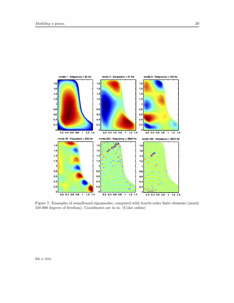
The soundboard model assumes a diagonal damping in the modal basis. Its motion is first decom-posed onto the modes of the undamped Reissner–Mindlin plate (see Eqs. (15)) belonging to theaudio range, after semi-discretization in space with higher-order finite elements[2]. In practice, 2400 modes are needed to model the soundboard vibrations up to 10 kHz. Fig. 7 shows some of thenumerically computed modes associated to their eigenfrequencies. The presence of ribs and bridgesis visible in the high frequency range. These modes are only computed once for all, before the timecomputation starts.
The choice of a Reissner-Mindlin model for the plate is validated numerically by comparisonwith measurements on rectangular plates made by other authors[33] (see Fig. 8). The discretemodal amplitudes Xh,n(t) of the discrete eigenmodes are solutions of the uncoupled second-orderequations:
d2Xh,n
dt2+ (2πfh,n)
2 Xh,n = Fh,n
where the fh,n are the numerically computed eigenfrequencies of the undamped Reissner–Mindlinmodel. We then introduce a discrete damping mode per mode:
d2Xh,n
dt2+ α(fh,n)
dXh,n
dt+ (2πfh,n)
2Xh,n = Fh,n (34)
This procedure yields decoupled equations which can be solved analytically in time, without intro-ducing any additional approximation or numerical dispersion[2]. The energy identity over time ofthis semi-discrete problem is also exactly satisfied with this method. However, one drawback ofthis choice is the loss of the local nature of the coupling with strings and air.
3.4 Strings-soundboard coupling at the bridge
The discrete formulation of the strings-soundboard continuity equations must be done with specialcare in order to ensure the stability of the resulting coupled scheme. The purpose here is to couplethe implicit three points nonlinear strings scheme described in Section 3.1 with the time semi-analytic soundboard model described in Section 3.3. In practice, the last point of the string has tofulfil a discrete condition consistent with the continuity condition expressed in Eq. (19).
RR n° 8181
Modeling a piano. 20
Figure 7: Examples of soundboard eigenmodes, computed with fourth-order finite elements (nearly450 000 degrees of freedom). Coordinates are in m. (Color online)
RR n° 8181

Modeling a piano. 21
Figure 8: Simulated and measured eigenfrequencies obtained for rectangular isotropic (left) and or-thotropic (right) plates. The simulated results are obtained for three boundary conditions: Dirichlet(circles), Neumann (squares) and simply supported (triangles) conditions. The experiments weredone on plates suspended by Nylon threads, and the results fit very well with the simulations us-ing Neumann (free) boundary conditions. As expected, the eigenfrequencies increase as the fixingconditions become stronger.
For computational efficiency reasons, new variables are introduced that represent the couplingforces associated to the cinematic conditions between string and soundboard expressed in Eq. (19)(see Fig. 4). The strings and soundboard unknowns are evaluated on interleaved time grids: n∆tfor the strings, and (n+ 1/2)∆t for the soundboard. The forces at the bridge are consideredconstant on time intervals of the form [(n− 1/2)∆t, (n+ 1/2)∆t]. The coupling condition is animplicit version of Eq. (19) centered on times n∆t (see Fig. 9).
Due to the linearity of the soundboard model, it is possible to express the soundboard unknownsas linear functions of the forces at the bridge. Taking advantage of this property, it is possible toperform Schur complements[15] on the system which, originally, is globally implicit. An algorithmis then written which updates first the unknowns of the strings and the forces at the bridge, and,in a second step, updates the unknowns of the soundboard.
3.5 Acoustic propagation and structural acoustics
The acoustic domain being unbounded, it is necessary to artificially truncate the computationaldomain, while minimizing the wave reflection on this artificial boundary. Perfectly Matched Layersis an option [16]. Even after this truncation, the numerical parameters need to be chosen smallenough, in view of the necessary wideband computation. A commonly accepted rule is to provide atleast 10 points per wavelength so that the signal is spatially well sampled by the discretization. Forexample, if one has to model the propagation of an acoustic wave with noticeable energy content upto 10 kHz, with a corresponding smallest wavelength of 3.4 cm, one has to provide a mesh composedof 3 mm large elements. Since the size of a piano can be 2 m large and 3 m long, with a 40 cm rim,the mesh reaches 60 millions of degrees of freedom.
RR n° 8181

Modeling a piano. 22
n n
n+ 1
n− 1n− 1
n+ 1
!"#$%&%'()*+,- ./0%1232$4'%& 50#$%&%'()*+,-
*67#$%389
:&679'%&();<- .673=>62?=()@(<- .'?%38()A(<-
9#/&'?2$(B%8B(6?=/?(+!C C6=2$(=/&60#69%'%63 D%8B(6?=/?(+!C
Xh,n(t)
Xh,n(t)
Xh,n(t)
Pn+1/2h
Pn−1/2h
Vna,h
Vn+1
a,h
Vn−1
a,h
(un
h, v
n
h,ϕ
n
h)
(un+1
h, v
n+1
h,ϕ
n+1
h)
(un−1
h, v
n−1
h,ϕ
n−1
h)
Figure 9: Schematic view of the discretization. The string’s variables (uh, vh, ϕh) are evaluated onthe time grid n ∆t. The soundboard modal displacements Xh,p are calculated at times (n+1/2) ∆t.The acoustic velocity Va,h is calculated at times n ∆t and the acoustic pressure Ph is calculated attimes (n + 1/2) ∆t. All methods used yield energy identities, where the energies are centered ontimes (n+1/2) ∆t. The coupling terms representing the forces at the bridge are centered on timesn ∆t. (Color online)
The acoustical problem is solved in space with higher-order finite elements, and in time withan explicit leapfrog scheme, in view of the large number of degrees of freedom to consider. Theacoustic velocity V a,h and sound pressure Ph are calculated at times n∆t and (n+ 1/2)∆t,respectively. This scheme has a restrictive stability condition: in practice, the adopted time step isaround 10−6 s. An implicit coupling exists between the soundboard displacement and the acousticpressure in the vicinity of the plate, which implies a change of basis between both the physicaland modal representations of the soundboard. In the variational formulation, the coupling betweensoundboard and air appears as skew–symmetric source terms for the soundboard and the soundpressure equations, respectively. These terms are constructed in the discrete scheme so that theyvanish when computing the energy, and centered at times n∆t. Due to the linearity of the equations,it is possible here to perform Schur complements, yielding an efficient algorithm that updatesseparately the plate (with a semi-analytic method) and the air variables.
RR n° 8181

Modeling a piano. 23
3.6 A virtual piano
The resulting numerical scheme is stable, under the previously mentioned conditions on the nu-merical parameters, globally implicit, nonlocal for the soundboard, and uses multifarious methods.The efficiency of the computer code is optimized through the use of adapted additional unknownsand Schur complements, so that the update of the unknowns of each subsystem is made separatelyat each time step. A massively parallel computing was necessary, and special attention was paidto the cost of each step, in order to minimize the global computation time. In average, computingone second of sound for the complete piano model (with frequency content up to 10 kHz) takes 24hours on a 300 cpus cluster (around 86 ms per time iteration for the complete piano).
In Fig. 10 the time evolution of selected quantities are represented for the note C2. Nearly 3 000degrees of freedom (dofs) are used on each string of the triplet, 420 000 dofs are used to computethe 2400 first modes of the soundboard, and slightly more than 90 000 000 dofs are used in the airdomain. The time step is 10−6 second. The parameters are listed in Table 1 for the soundboardand in Table 3 for the strings. The hammer strikes the strings with a velocity of 4.5 m·s−1 (a forteto fortissimo playing). The longitudinal precursor can be seen on the upper parts of the figure:when the longitudinal wave of the string reaches the bridge, the soundboard is pushed down (seeFig. 10(b)), until the transverse wave arrives and pulls the soundboard up (see Fig. 10(g)). Theacoustic wave is absorbed by the PML (not represented in the figures), and the rim is an obstacleto sound propagation (see Fig. 10(h)). Fig. 11 shows the energy evolution of each subsystem versustime, both in linear and logarithmic scales. The energy associated to sound propagation is computedin the truncated domain only. The total energy (solid line) is decreasing, as expected.
4 Results of the simulations
In order to show the ability of the method to simulate the complete register of a piano, the results(output data) of the model are presented and discussed in this Section for different notes in thelow (D♯1 and C2), medium (F3) and treble (C♯5 and G6) register, respectively. Table 3 gives thenumerical values used for these notes in the simulations.
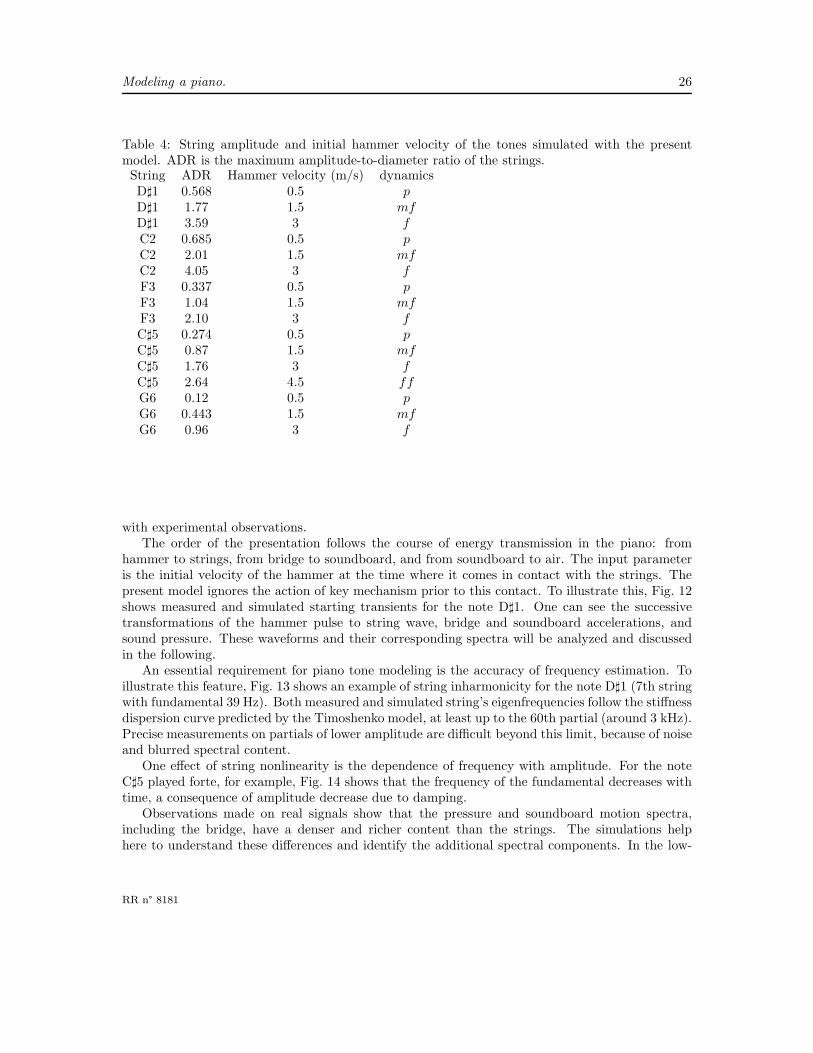
Since the nonlinear string is one major feature of the model, particular attention is paid to theinfluence of string amplitude on the resulting sound. The amplitude of transverse string motionis linked to the impact velocity of the hammer. The string amplitudes of the simulated tones,normalized with respect to string diameter, and the associated hammer impact velocities are shownin Table 4. Comparisons with real tones allows to group the simulations into typical categories ofplaying: piano, mezzo-forte, forte, fortissimo, corresponding to realistic, though relatively arbitrary,hammer velocity ranges[34].
As a rule of thumb, it is generally admitted that, for thin structures, nonlinear effects becomeapparent when the amplitude of the vibrations are comparable to the thickness[35]. Transposing
this rule to the case of strings yields the condition ADR =|us|
ds> 1, where ds is the diameter of the
string. According to this rule, Table 4 predicts that nonlinear effects should be noticeable in thebass and medium ranges, even for moderate hammer velocity, whereas they should be less easilydetectable for the treble notes, except for strong impacts. This simple criterion is in accordance
RR n° 8181

Modeling a piano. 24
Figure 10: Time evolution of some variables of the piano model for string C2. The transversedisplacement of the string is represented in the upper parts of the figures, while the longitudinaldisplacement is shown through shading in the string thickness (upper scale). The displacement ofthe soundboard is shown in the lower parts, while the pressure is shown in two vertical planes whichcross at the point where the string is attached to the bridge: x = 0.59 m and y = 1.26 m. Thelower scale is related to the sound pressure. The scale of the soundboard’s displacement is adjustedover time in order to see the evolution of waves clearly. (a) t = 0.4 ms. (b) t = 1.1 ms. (c) t = 2.1ms. (d) t = 3.1 ms. (e) t = 4.1 ms. (f) t = 5.1 ms. (g) t = 7.1 ms. (h) t = 8.1 ms. (i) t = 16.1 ms.(Color online)
RR n° 8181

Modeling a piano. 25
0 0.01 0.02 0.03 0.04-10
-8
-6
-4
-2
0
Time (s)0 0.01 0.02 0.03 0.04
0
0.02
0.04
0.06
0.08
0.1
Time (s)
Figure 11: Energy vs time for note C2 (three strings). Solid line: Total energy. [- -] Hammer. [- ·]Strings. [· · ·] Soundboard. [Thick -] Air. Left: Linear scale. Right: Logarithmic scale.
Table 3: Parameters used for the strings in the simulationsNote D♯1 C2 F3 C♯5 G6
L (m) 1.945 1.600 0.961 0.326 0.124d (mm) 1.48 0.9502 1, 0525 0, 921 0.794F 5.73 3.55 1 1 1T0 (N) 1781 865 774 684 587f0 (Hz) 38.9 65.4 174.6 555.6 1571.4p 2.4 2.27 2.4 2.6 3.0
KH (N·m−p) 4.0× 10⁸ 2× 10⁹ 1.0× 10⁹ 2.8× 10¹⁰ 2.3× 10¹¹
MH (g) 12.00 10.20 9.00 7.90 6.77
xH (m) 0.25 0.2 0.115 0.039 0.015x0 (m) 0.47 0.59 0.54 0.88 1.16y0 (m) 1.63 1.26 0.83 0.23 0.05
A =πd2
4, I =
πd4
64, E = 2.0× 10¹¹ Pa, G = 8× 10¹⁰ Pa, ρc = 7850 kg.m−3, ρ = ρcF.
RR n° 8181
Modeling a piano. 26
Table 4: String amplitude and initial hammer velocity of the tones simulated with the presentmodel. ADR is the maximum amplitude-to-diameter ratio of the strings.String ADR Hammer velocity (m/s) dynamicsD♯1 0.568 0.5 pD♯1 1.77 1.5 mfD♯1 3.59 3 fC2 0.685 0.5 pC2 2.01 1.5 mfC2 4.05 3 fF3 0.337 0.5 pF3 1.04 1.5 mfF3 2.10 3 fC♯5 0.274 0.5 pC♯5 0.87 1.5 mfC♯5 1.76 3 fC♯5 2.64 4.5 ffG6 0.12 0.5 pG6 0.443 1.5 mfG6 0.96 3 f
with experimental observations.The order of the presentation follows the course of energy transmission in the piano: from
hammer to strings, from bridge to soundboard, and from soundboard to air. The input parameteris the initial velocity of the hammer at the time where it comes in contact with the strings. Thepresent model ignores the action of key mechanism prior to this contact. To illustrate this, Fig. 12shows measured and simulated starting transients for the note D♯1. One can see the successivetransformations of the hammer pulse to string wave, bridge and soundboard accelerations, andsound pressure. These waveforms and their corresponding spectra will be analyzed and discussedin the following.
An essential requirement for piano tone modeling is the accuracy of frequency estimation. Toillustrate this feature, Fig. 13 shows an example of string inharmonicity for the note D♯1 (7th stringwith fundamental 39 Hz). Both measured and simulated string’s eigenfrequencies follow the stiffnessdispersion curve predicted by the Timoshenko model, at least up to the 60th partial (around 3 kHz).Precise measurements on partials of lower amplitude are difficult beyond this limit, because of noiseand blurred spectral content.
One effect of string nonlinearity is the dependence of frequency with amplitude. For the noteC♯5 played forte, for example, Fig. 14 shows that the frequency of the fundamental decreases withtime, a consequence of amplitude decrease due to damping.
Observations made on real signals show that the pressure and soundboard motion spectra,including the bridge, have a denser and richer content than the strings. The simulations helphere to understand these differences and identify the additional spectral components. In the low-
RR n° 8181

Modeling a piano. 27
-1 0 1 2 3 4 5 6 7 8 9-1000
0100020003000
Hammer Acceleration (m / s2)
time (ms)-1 0 1 2 3 4 5 6 7 8 9
-500
0
500
1000
1500Hammer Acceleration (m / s2)
time (ms)
0 0.05 0.1 0.15
0
time (s)
String displacement (AU)
0 0.05 0.1 0.15-2
0
2x 10
-3
time (s)
String displacement (m)
0 0.05 0.1 0.15-40
-20
0
20
40
time (s)
Bridge acceleration (m / s2)
0 0.05 0.1 0.15-20
0
20
time (s)
Bridge acceleration (m / s2)
0 0.05 0.1 0.15-50
0
50
time (ms)
Soundboard acceleration (m / s2)
0 0.05 0.1 0.15-20
0
20
time (s)
Soundboard acceleration (m / s2)
0 0.05 0.1 0.15-6-4-2
024
time (s)
Pressure (Pa)
0 0.05 0.1 0.15-5
0
5
time (s)
Pressure (Pa)
Figure 12: Measured (left) and simulated (right) starting transients of the main variables for noteD♯1 (7th). From top to bottom: hammer acceleration, string displacement (at point located 1.749m from the agraffe), bridge acceleration at string end, soundboard acceleration (at point x=0.17 m; y=1.49 m in the coordinate axes shown in Fig. 3), sound pressure (simulated at point x=0.8500; y=1.4590 ; z=0.3800, and measured in the nearfield at a comparable location).
frequency range, most of the additional spectral peaks correspond to soundboard modes excitedby the string pulse. They are present in piano sounds even for light touch. These modes areparticularly visible for the upper notes of the instrument, because of large spacing between thestrings’ partials (see Fig. 15). The soundboard modes are damped more rapidly than the string’spartials, and thus they are essentially audible during the initial transients of the tones.
Increasing the hammer velocity progressively induces additional peaks between the string com-ponents, a consequence of string nonlinearity and coupling at the bridge. As explained in Section2, a coupling exists between transverse and longitudinal motion of the nonlinear string. Due tostring-bridge coupling, both the transverse and longitudinal components are transmitted to thesoundboard. This explains why the longitudinal eigenfrequencies of the strings are visible on bridgeand soundboard waveforms, but not on the transverse string motion[7]. In addition, a consequenceof the nonlinear terms in the string wave equation is that combinations of string components arecreated: the so-called “phantom partials”[6].
As explained theoretically from Eq. 21 in Section 2, the frequencies of these phantoms correspond
RR n° 8181

Modeling a piano. 28
0 20 40 60 80-0.05
0
0.05
0.1
0.15
Rank of partials
∆ f/
(n f
1)
Figure 13: Inharmonicity derived from frequency analysis of simulated (black circles) and measured(squares) string spectra. Note D♯1.
0.01 0.1 1 10554
556
558
560
Time (s) ->
Freq
uenc
y (H
z) -
>
Figure 14: Evolution of frequency with time of the fundamental, due to geometrical nonlinearity.Simulation of note C♯5 played fortissimo.
RR n° 8181
Modeling a piano. 29
!"#$%&'(
)*$+,$-./%&01(
234 235 236 2372
522
8222
8522
9222
!852
!822
!52
2
!"#$%&'(
)*$+,$-./%&01(
234 235 236 237 2382
722
9222
9722
4222
!972
!922
!72
2
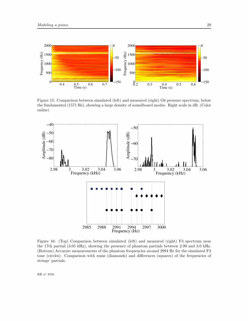
Figure 15: Comparison between simulated (left) and measured (right) G6 pressure spectrum, belowthe fundamental (1571 Hz), showing a large density of soundboard modes. Right scale in dB. (Coloronline)
!"#$ % %"&! %"&' %"&(
!$&
!)&
!(&
!*&
!'&
+,-./-012345678
9:;<=>/?-34?@8
!"#$ % %"&! %"&' %"&(
!)&
!(&
!*&
+,-./-012345678
9:;<=>/?-34?@8
2985 2988 2991 2994 2997 3000Frequency (Hz)
Figure 16: (Top) Comparison between simulated (left) and measured (right) F3 spectrum nearthe 17th partial (3.05 kHz), showing the presence of phantom partials between 2.99 and 3.0 kHz.(Bottom) Accurate measurements of the phantom frequencies around 2994 Hz for the simulated F3tone (circles). Comparison with sums (diamonds) and differences (squares) of the frequencies ofstrings’ partials.
RR n° 8181

Modeling a piano. 30
0 2 4 6 8 100
2
4
6
8
10
12
Frequency (kHz)
Dam
ping
fac
tors
(s-1
)
Figure 17: Damping factors of the partials due to radiation (squares), radiation and soundboardlosses (circles), radiation, soundboard and string losses (triangles), and for all causes of losses(diamonds). Simulations of note C♯5.
to sums (or differences) between two or three of the string components, depending on whether thecombinations are the results of quadratic, or cubic, nonlinearities. In general all combinationsare not observable, and obey to complex rules. The instability conditions that gives rise to thesecomponents must reach a certain threshold[35]. Similar phenomena are observed in gongs andcymbals[36]. Such an analysis is beyond the scope of this paper. Notice in Fig. 16 that thefrequencies predicted by sums or differences of partials’ eigenfrequencies correspond with greataccuracy (less than 1 Hz) to the observed phantoms, both in simulations and measurements.
In the time-domain, the presence of nonlinear coupling is seen in the precursors. Fig. 12 showsthat the precursor is not visible on the string displacement, while it is clearly seen on the otherwaveforms (bridge, soundboard, pressure), both in measurements and simulations. This precursoris primarily due to the longitudinal waves. In real instruments, the composition of these precursorsis more complex and not totally understood[5]. Presumably, they contain some signature of shockof the key on the keybed, and other structural components that are not yet included in our model.
One further interest of simulations lies in the possibility of separating phenomena that aremixed together in the reality. In this respect, damping factors of the partials are good illustratingexamples. When systems are coupled, it is always problematic to separate the causes of losses.In contrast, a model has the capability of introducing dissipation of energy in the hammer felt,along the string, and at the ends, separately. Even more interesting is the separation of structuraland radiation losses. Experimentally, such a separation would require a rather delicate procedurewhere the instrument should to be put in a vacuum chamber in order to modify the conditionsof radiation. One known difficulty of such experiments follows from the modifications of woodproperties consecutive to variations of ambient pressure, and thus investigating such a problemwith the help of simulations is an appealing alternative. To illustrate this ability of the model,Fig. 17 shows the damping factors derived from simulations for the C♯5 note, introducing each
RR n° 8181

Modeling a piano. 31
cause of losses successively (radiation, soundboard, strings, hammer felt). These damping factorsare averaged in the frequency band of each partial, during the first second of the simulated tones.The damping factor related to the 17th partial (around 7 kHz) is ignored, since its amplitude isvery low due to the striking position. In this example, the influence of the soundboard seems tobe weak. For some partials, it turns also paradoxically out that the mean damping factors is lessin the presence of both soundboard losses and radiation than for radiation only. In fact, it mightbe plausible that the conditions of coupling between strings and soundboard modes are slightlymodified by the damping due to eigenfrequency shift. As a consequence, a “local” measure ofdamping might exhibit unexpected results. More investigation is needed here based, for example,on the computation of sound power and radiation efficiency.
5 Conclusion
In this paper, a global model of a grand piano has been presented. This model couples together thehammer, the nonlinear strings, the soundboard with ribs and bridges, and the radiation of acousticwaves in free field. As far as we are aware, this is probably the most general physical model of apiano available today. However, a number of significant features of real pianos were not consideredin this model. The key mechanism, and an accurate description of the hammer action includingthe vibrations of the hammer shank, have been left aside. From the point of view of the player,adding this part would allow interesting studies of the links between the action of the finger andthe resulting sound.
Beside this, an improvement in the string model would be to account for the nonplanar motionobserved on real pianos. A strong hypothesis is that this motion might be due to the customaryobserved zig-zag clamping conditions at the bridge[37], but this needs to be verified and quantifiedby measurements. To reproduce such effects, more appropriate boundary conditions have to bedeveloped, that allow the progressive transformation of a vertical polarization into an horizontalmotion. The way both polarizations are transmitted to the rest of the structure also need tobe better understood. The coexistence of these polarizations with different decay times greatlyinfluence the amplitude envelope of the tone, and thus its perception.
The motion of the structure is restricted here to the soundboard. Previous measurements tendto show that some other parts of the instrument contribute to the sound[5]. In this context, itwould be attractive to reproduce the shock of the key against the keybed and the vibrations of therim, to evaluate their relevance.
The present model is solved in the time-domain. The results yield the temporal evolution of themain significant variables of the system simultaneously: hammer force, string motion, bridge andsoundboard vibrations, pressure field. The obtained waveforms can be heard through headphonesor loudspeakers, and clearly evoke piano tones. They also shed useful light on the transfer of energyand transformations of the signals from hammer to strings, soundboard and air.
To numerically solve the problem, specific and original methods were developed for each part ofthe piano. A gradient approach coupled to higher-order finite elements lead us to design an energydecaying numerical scheme for the string’s system, which is nonlinearly coupled to the hammer. Amodal method was chosen to solve the soundboard problem, with a diagonal damping form. Theeigenmodes and eigenfrequencies are computed once for all using higher-order finite elements, andan analytic formula is then used in time. Finally, sound radiation is solved with finite differencesin time and higher-order finite elements in the space domain, which is artificially truncated withPML (Perfectly Matched Layers).
RR n° 8181

Modeling a piano. 32
As a result, a numerical formulation of the global piano model is obtained with high precision intime, space and frequency. This formulation ensures that the total energy of the system is decaying.The model accounts for the dependence of piano sounds and vibrations with amplitude, due tononlinear modeling of strings and hammers. In this respect, the simulations show the main effectsof nonlinearity observed on real tones: precursors, time evolution of eigenfrequencies, transverse-longitudinal coupling, and phantom partials. The model used for string-soundboard coupling atthe bridge is consistent with the transmission of nonlinearities observed on real instruments. Dueto this coupling, the presence of the soundboard modes in the piano transients are reproduced ina natural way. The soundboard model also integrates the presence of ribs and bridges, which aretreated as heterogeneities in material and thickness of a Reissner-Mindlin plate.
The piano is a instrument with a large register. Most of the notes, from bass to treble, showa wideband spectrum, with significant energy up to 10 kHz and more. As a consequence, pianomodeling requires a fine spatial grid for each part. The most demanding grid is associated with themodeling of the pressure field. This part of the simulations was a particularly challenging pointof the work, which necessitated high performance parallel computing. In the present state of theequipment, several hours of computation in parallel on a 300 cpus cluster are necessary to computethe pressure field during one second in a box of the order of 10 m3 that contains the instrument[38].
Analysis of the simulated piano tones in time and frequency show a satisfactory agreement withmeasurements performed on a Steinway D grand piano. This particular instrument was used forextracting accurate values of input parameters, thus allowing precise comparisons between modeland measurements for some selected notes in the bass, medium and treble range. Informal auditoryevaluation of the simulated tones indicates that medium and treble notes are fairly well reproduced,but that the depth of the bass notes is not completely rendered.
In its present state, this model of piano should be considered as a crude skeleton of the in-strument. Its prime function is to get a better understanding of the complex coupled phenomenainvolved in a complete piano, with the possibility of systematic variations of making parameters.Numerous additional improvements, careful adjustments and fine tuning would be necessary beforethinking of competing with high-quality pianos. However, even in its imperfect form, we believethat the model could be used as a companion tool for piano making. In this context, investigatingthe influence of soundboard modifications on the radiation of sound and on string-bridge couplingappear as potentially fruitful examples.
6 Acknowledgment
Simulations presented in this paper were carried out using the PLAFRIM experimental testbed,being developed under the Inria PlaFRIM development action with support from LABRI andIMB and other entities: Conseil Regional d’Aquitaine, FeDER, Universite de Bordeaux and CNRS(see https://plafrim.bordeaux.inria.fr/) and the computing facilities MCIA (Mesocentre de CalculIntensif Aquitain) of the Universite de Bordeaux and of the Universite de Pau et des Pays de l’Adour(see http://www.mcia.univ-bordeaux.fr).
References
[1] N. Giordano and M. Jiang, “Physical modeling of the piano”, Eurasip Journal on Appl. SignalProc. 7, 926–933 (2004).
RR n° 8181

Modeling a piano. 33
[2] G. Derveaux, A. Chaigne, P. Joly, and E. Becache, “Time-domain simulation of a guitar:Model and method”, J. Acoust. Soc. Am. 114, 3368–3383 (2003).
[3] L. Rhaouti, A. Chaigne, and P. Joly, “Time-domain modeling and numerical simulation of akettledrum”, J. Acoust. Soc. Am. 105, 3545–3562 (1999).
[4] S. Bilbao, “Conservative numerical methods for nonlinear strings”, J. Acoust. Soc. Am. 118,3316–3327 (2005).
[5] A. Askenfelt, “Observations on the transient components of the piano tone”, STL-QPSR 34,15–22 (1993).
[6] Harold A. Conklin, Jr., “Generation of partials due to nonlinear mixing in a stringed instru-ment”, J. Acoust. Soc. Am. 105, 536–545 (1999).
[7] N. Giordano and A. J. Korty, “Motion of a piano string: Longitudinal vibrations and the roleof the bridge”, J. Acoust. Soc. Am. 100, 3899–3908 (1996).
[8] Harold A. Conklin, Jr., “Design and tone in the mechanoacoustic piano. part II. Piano struc-ture”, J. Acoust. Soc. Am. 100, 695–708 (1996).
[9] E. Balmes, “Modeling damping at the material and structure level”, in Proceedings of the24th IMAC Conference and exposition on structural dynamics, volume 3, 1314–39 (Society forExperimental Mechanics, St Louis, Missouri) (2006).
[10] H. Jarvelainen, V. Valimaki, and M. Karjalainen, “Audibility of the timbral effects of inhar-monicity in stringed instrument tones”, Acoustics Research Letters Online 2, 79–84 (2001).
[11] B. Bank and H.-M. Lehtonen, “Perception of longitudinal components in piano string vibra-tions”, J. Acoust. Soc. Am. 128, EL117–EL123 (2010).
[12] A. Chaigne and A. Askenfelt, “Numerical simulation of piano strings. I. A physical model fora struck string using finite-difference methods”, J. Acoust. Soc. Am. 95, 1112–1118 (1994).
[13] P. Morse and K. Ingard, Theoretical Acoustics, chapter 14, 856–863, (Princeton UniversityPress, Princeton, New Jersey) (1968).
[14] Harold A. Conklin, Jr., “Design and tone in the mechanoacoustic piano. part III. Piano stringsand scale design”, J. Acoust. Soc. Am. 100, 1286–1298 (1996).
[15] C. Brezinski, Schur complements and applications in numerical analysis, Vol. 4 of Numericalmethods and algorithms, chapter 7, 227–258 (Springer, New York) (2005).
[16] E. Becache, S. Fauqueux and P. Joly, “Stability of perfectly matched layers, group velocitiesand anisotropic waves” Journal of Computational Physics, 188, 399-403 (2003).
[17] J. Chabassier and S. Imperiale, “Stability and dispersion analysis of improved time discretiza-tion for simply supported prestressed Timoshenko systems. Application to the stiff pianostring.”, Wave Motion, doi:10.1016/j.wavemoti.2012.11.002 (2012).
[18] H. Fletcher, “Normal vibration frequencies of a stiff piano string”, J. Acoust. Soc. Am. 36,203–209 (1964).
RR n° 8181

Modeling a piano. 34
[19] J. Bensa, S. Bilbao, and R. Kronland-Martinet, “The simulation of piano string vibration:From physical models to finite difference schemes and digital waveguides”, J. Acoust. Soc.Am. 114, 1095–1107 (2003).
[20] J. Chabassier, A. Chaigne, and P. Joly, “Time domain simulation of a piano. Part I: modeldescription.”, Research Report 8097, INRIA, Bordeaux, France (2012).
[21] G. Weinreich, “Coupled piano strings”, J. Acoust. Soc. Am. 62, 1474–1484 (1977).
[22] A. Stulov, “Dynamic behavior and mechanical features of wool felt”, Acta Mechanica 169,13–21 (2004).
[23] N. Giordano and J. P. Winans II, “Piano hammers and their force compression characteristics:does a power law make sense ?”, J. Acoust. Soc. Am. 107, 2248–2255 (2000).
[24] P. H. Bilhuber and C. A. Johnson, “The influence of the soundboard on piano tone quality”,J. Acoust. Soc. Am. 11, 311–320 (1940).
[25] A. Mamou-Mani, J. Frelat, and C. Besnainou, “Numerical simulation of a piano soundboardunder downbearing”, J. Acoust. Soc. Am. 123, 2401–2406 (2008).
[26] T. K. Hasselman, “Modal coupling in lightly damped structures”, AIAA Journal 14, 1627–1628(1976).
[27] K. Ege, X. Boutillon, and M. Rebillat, “Vibroacoustics of the piano soundboard:(non)linearityand modal properties in the low- and mid-frequency ranges”, J. Sound Vib. 335, 1288–1305(2013).
[28] M. Podlesak and A. R. Lee, “Dispersion of waves in piano strings”, J. Acoust. Soc. Am. 83,305–317 (1988).
[29] J. Cuenca and R. Causse, “Three-dimensional interaction between strings, bridge and sound-board in modern piano’s treble range”, in Proc. of the 19th International Congress on Acoustics,edited by SEA, volume 3, 1705–1710 (Madrid, Spain) (2007).
[30] J. Chabassier, A. Chaigne, and P. Joly, “Transitoires de piano et non-linearites des cordes: Mesures et simulations”, in Proceedings of the 10th French Acoustical Society Meeting (inFrench), 225 (Lyon, France) (2010).
[31] B. Bank and L. Sujbert, “Generation of longitudinal vibrations in piano strings: From physicsto sound synthesis”, J. Acoust. Soc. Am. 117, 2268–2278 (2005).
[32] J. Chabassier and P. Joly, “Energy preserving schemes for nonlinear Hamiltonian systems ofwave equations. Application to the vibrating piano string.”, Computer Methods in AppliedMechanics and Engineering 199, 2779–2795 (2010).
[33] C. Lambourg, “Modele temporel pour la simulation numerique de plaques vibrantes. applica-tion a la synthese sonore”, Ph.D. thesis, Universite du Maine (1997).
[34] A. Askenfelt and E. Jansson, “From touch to string vibrations: II: The motion of key andhammer”, J. Acoust. Soc. Am. 90, 2383–2393 (1991).
RR n° 8181

Modeling a piano. 35
[35] A. H. Nayfeh and D. T. Mook, Nonlinear oscillations, chapter 7, 485-499, Wiley classicslibrary (J. Wiley, Hoboken, New Jersey) (1979).
[36] C. Touze and A. Chaigne, “Lyapunov exponents from experimental time series: Applicationto cymbal vibrations”, Acustica united with Acta Acustica 86, 557–567 (2000).
[37] R. Anderssen and W. D. Stuart, “The challenge of piano maker”, The Math. Scientist 32,71–82 (2007).
[38] J. Chabassier and M. Durufle, “Physical parameters for piano modeling”, Technical reportRT-0425, INRIA, Bordeaux, France (2012).
RR n° 8181

RESEARCH CENTRE
BORDEAUX – SUD-OUEST
200 Avenue de la Vieille Tour,
33405 Talence Cedex
Publisher
Inria
Domaine de Voluceau - Rocquencourt
BP 105 - 78153 Le Chesnay Cedex
inria.fr
ISSN 0249-6399

Modeling a piano. 36
RR n° 8181