Modeling and Performance Improvementof TCP over LTE Handover

MATTEO PACIFICO

Master’s Degree ProjectStockholm, Sweden 2009

CHAOOCHAOOCHAOO

“con tanto amore mi avete cresciuto,con uno sguardo mi avete insegnato a vivere,

con un sorriso mi avete reso felice,con coraggio avete accettato e sostenuto le mie scelte,

con tanta pazienza mi avete permesso di diventare quel che sono ora.Siete per sempre nel mio cuore!”

A Mamma e Papa

Abstract

The Long Term Evolution (LTE) of the UMTS Terrestrial Radio Access and

Radio Access Network is a new communication standard aimed for commercial

deployment in 2010. Goals for LTE include support for improved system capacity

and coverage, high peak data rates, low latency, reduced operating costs, multi-

antenna support, flexible bandwidth operations and seamless integration with

existing systems.

The aim of this thesis project is to study the impacts on the end-user and sys-

tem performance when users with high bit rates tcp services are moving through

the network. These impacts affect the reduced end-user or system throughput,

e.g., due to congestion in the transport network, leading to poor utilization of

the transport and radio resources available. To reach such an aim, it has been

necessary (1) to create a new simulator with the ns-2 and perform simulation in

different network settings and (2) formulate a mathematical model able to cap-

ture the principal dynamics of the real system. Possible solutions to mitigate the

impacts are investigated by comparing the simulations results of tcp performance

in the radio and transport network, with the mathematical model of it.

The project has been performed at the Automatic Control Lab at KTH in

Stockholm and in collaboration with Ericsson Research Lab. The work is part of a

joint effort with Davide Pacifico. Further results are available in the master thesis

“Analysis and Performance Improvement of tcp during handover of LTE”[1].

iii

Preface

LTE, short for Long Term Evolution, is the result of ongoing work by the 3rd

Generation Partnership Project (3GPP), a collaborative group of international

standards organizations and mobile-technology companies. 3GPP set out in 1998

to define the key technologies for the third generation of GSM-based mobile net-

works (3G), and its work has continued to define the ongoing evolution of these

networks. Near the end of 2004, discussions on the longer-term evolution of 3G

networks began, and a set of high-level requirements for LTE was defined: the

networks must transmit data at a reduced cost per bit compared to 3G; they must

be able to offer more services at lower transmission cost with better user expe-

rience; LTE must have the flexibility to operate in a wide number of frequency

bands; it should utilize open interfaces and offer a simplified architecture; and

it must have reasonable power demands on mobile terminals. Standardization

work on LTE is continuing with some operators projected to deploy the first LTE

networks in 2009.

LTE (“Turbo 3G”), is a wireless broadband technology designed to support

roaming Internet access via cell phones and handheld devices. Because LTE offers

significant improvements over older cellular communication standards, some refer

to it as a 4G (fourth generation) technology along with WiMax.

LTE defines new radio connections for mobile networks, and will utilize Or-

thogonal Frequency Division Multiplexing (OFDM), a widely used modulation

v

Preface

technique that is the basis for Wi-Fi, WiMAX, and the Digital Video Broadcast-

ing (DVB) and Digital Audio Broadcasting (DAB) technologies. The targets for

LTE indicate bandwidth increases as high as 100 Mbps on the downlink, and up

to 50 Mbps on the uplink. However, this potential increase in bandwidth is just

a small part of the overall improvement LTE aims to provide. LTE is optimized

for data traffic, and it will not feature a separate, circuit-switched voice network,

as in 2G GSM and 3G UMTS networks.

LTE is the successor to the current generation of UMTS 3G technology, which

is based upon WCDMA (3G), HSDPA, HSUPA, and HSPA. LTE is not a replace-

ment for UMTS in the way that UMTS was a replacement for GSM, but rather

an update to the UMTS technology that will enable it to provide significantly

faster data rates for both uploading and downloading.

With its architecture centered on Internet Protocol (IP), Long Term Evolution

promises to have excellent support for browsing Web sites, VoIP and other IP-

based services. LTE can theoretically support downloads at 100 Megabits per

second (Mbps) or more based on experimental trials.

Another important feature of LTE is the amount of flexibility it allows opera-

tors in determining the spectrum in which it will be deployed. Not only will LTE

have the ability to operate in a number of different frequency bands (meaning op-

erators will be able to deploy it at lower frequencies with better propagation char-

acteristics), but it also features scalable bandwidth. Whereas WCDMA/HSPA

uses fixed 5 MHz channels, the amount of bandwidth in an LTE system can be

scaled from 1.25 to 20 MHz. This means networks can be launched with a small

amount of spectrum, alongside existing services, and adding more spectrum as

users switch over. It also allows operators to tailor their network deployment

strategies to fit their available spectrum resources, and not have to make their

spectrum fit a particular technology.

vi

Preface

The Transmission Control Protocol (tcp) is one of the core protocols of the

Internet Protocol Suite. TCP is so central that the entire suite is often referred

to as tcp/ip. tcp has been optimized for wired networks. Any packet loss is

considered to be the result of congestion and the congestion window size is reduced

dramatically as a precaution. However, wireless links are known to experience

sporadic and usually temporary losses due to fading, shadowing, handoff, and

other radio effects, that cannot be considered congestion. After the (erroneous)

back-off of the congestion window size, due to wireless packet loss, there can be

a congestion avoidance phase with a conservative decrease in window size. This

causes the radio link to be under utilized. Extensive research has been done

on the subject of how to combat these harmful effects. Suggested solutions can

be categorized as end-to-end solutions (which require modifications at the client

and/or server), link layer solutions, or proxy based solutions, which require some

changes in the network without modifying end nodes.

In cellular telecommunications, the term handoff refers to the process of trans-

ferring an ongoing call or data session from one channel connected to the core

network to another. The British English term for transferring a cellular call is

handover, which is the terminology standardized by 3GPP within such European

originated technologies as GSM and UMTS.

The aim of this thesis is to study the performances of the tcp protocol in the

handover procedure in LTE. This study proposes a mathematical model of that

features a compromise between simplicity and accuracy in the representation of

the dynamics of the real system.

The handover of an end-user who moves in a train or a bus or walks in a

crowded street while is surfing on internet by his terminal could be an abrupt

service interruptions. It is therefore important that the operator control properly

the handover procedure to avoid these problems.

vii

Preface

For these reasons is essential put the attention to mitigate the problems of

TCP during the handover and find a way to keep it transparent to the end-users.

To reach this aim, our analytical model is compared with a set of simulations of

the real network scenario performed by an original LTE simulation implemented

the ns-2 environment.

The thesis at a glance

This thesis work is organized in five chapters.

Chapter 1 is an overview of the LTE system and its main new features, such as

the system architecture, the Hybrid Automatic Repeat reQuest and the Evolved

RAN. A section is dedicated to LTE handover in which the procedure is explained

in detail.

In Chapter 2 the tcp protocol is described and its combination with LTE. In

particular we focus our attention on the tcp Reno.

In Chapter 3 we investigate problems arising during the handover procedure

in LTE network and we will show how to solve or mitigate it. We introduce

also an ns-2 network simulator and how it is implemented to realize our LTE

simulations.

In Chapter 5 we develop a model of TCP during handover, which is based

on the Joint link model proposed by Moller in 2008 [2]. This model shows the

behavior of the TCP congestion window of a mobile that does the LTE handover

procedure.

Finally in Chapter 6, we discuss the results and propose some developments

for future studies.

viii

Contents

Abstract iii

Preface v

Contents xi

List of Figures xiv

List of Tables xv

Abbreviations xvii

1 Background 3

1.1 LTE (Long Term Evolution) . . . . . . . . . . . . . . . . . . . . . 3

1.1.1 Requirements and performance goals for LTE . . . . . . . 4

1.1.2 System architecture description . . . . . . . . . . . . . . . 8

1.1.3 Key Features . . . . . . . . . . . . . . . . . . . . . . . . . 10

1.1.4 Network Sharing . . . . . . . . . . . . . . . . . . . . . . . 11

1.2 Mobility management . . . . . . . . . . . . . . . . . . . . . . . . . 17

1.3 LTE Technologies . . . . . . . . . . . . . . . . . . . . . . . . . . . 18

1.3.1 OFDM . . . . . . . . . . . . . . . . . . . . . . . . . . . . . 18

1.3.2 Multiple antenna techniques . . . . . . . . . . . . . . . . . 19

1.3.3 Scheduling . . . . . . . . . . . . . . . . . . . . . . . . . . . 24

1.4 Handover . . . . . . . . . . . . . . . . . . . . . . . . . . . . . . . 24

1.5 Summary . . . . . . . . . . . . . . . . . . . . . . . . . . . . . . . 28

ix

Contents

2 TCP and LTE 29

2.1 Importance of TCP . . . . . . . . . . . . . . . . . . . . . . . . . . 30

2.2 TCP key features . . . . . . . . . . . . . . . . . . . . . . . . . . . 31

2.2.1 Flow control . . . . . . . . . . . . . . . . . . . . . . . . . . 31

2.3 TCP Applicability . . . . . . . . . . . . . . . . . . . . . . . . . . 33

2.3.1 Congestion control . . . . . . . . . . . . . . . . . . . . . . 35

2.3.2 Explicit Congestion Notification (ECN) . . . . . . . . . . . 39

2.4 Evaluation of TCP Performance . . . . . . . . . . . . . . . . . . . 40

2.5 Bottleneck in the core network . . . . . . . . . . . . . . . . . . . . 42

2.5.1 GPRS Tunneling Protocol (GTP) . . . . . . . . . . . . . . 42

2.6 Summary . . . . . . . . . . . . . . . . . . . . . . . . . . . . . . . 45

3 Management of LTE handover 47

3.1 Forwarding procedure . . . . . . . . . . . . . . . . . . . . . . . . . 47

3.1.1 Optimal case . . . . . . . . . . . . . . . . . . . . . . . . . 49

3.1.2 Window halving case . . . . . . . . . . . . . . . . . . . . . 49

3.1.3 Timeout occurrence case . . . . . . . . . . . . . . . . . . . 50

3.2 Two improving solutions . . . . . . . . . . . . . . . . . . . . . . . 54

3.2.1 Advancing the path switch command . . . . . . . . . . . . 54

3.2.2 Predicting the handover occurrence . . . . . . . . . . . . . 55

3.3 Validation of the solutions . . . . . . . . . . . . . . . . . . . . . . 56

3.4 Summary . . . . . . . . . . . . . . . . . . . . . . . . . . . . . . . 59

4 LTE simulator: an overview 61

4.1 LTE simulator through ns-2 and nsMiracle . . . . . . . . . . . . . 61

4.2 Network topology . . . . . . . . . . . . . . . . . . . . . . . . . . . 64

4.3 Summary . . . . . . . . . . . . . . . . . . . . . . . . . . . . . . . 65

x

Contents

5 Mathematical model of TCP over LTE 67

5.1 Existing models . . . . . . . . . . . . . . . . . . . . . . . . . . . . 68

5.2 Model adaptation . . . . . . . . . . . . . . . . . . . . . . . . . . . 70

5.2.1 Single flow and multiple flow model . . . . . . . . . . . . . 72

5.3 Application scenario . . . . . . . . . . . . . . . . . . . . . . . . . 73

5.3.1 Handover preparation . . . . . . . . . . . . . . . . . . . . . 73

5.3.2 Handover actuation . . . . . . . . . . . . . . . . . . . . . . 74

5.3.3 Handover completion . . . . . . . . . . . . . . . . . . . . . 74

5.4 Simulations and Results . . . . . . . . . . . . . . . . . . . . . . . 75

5.5 Summary . . . . . . . . . . . . . . . . . . . . . . . . . . . . . . . 78

6 Conclusion and future work 79

6.1 Conclusion . . . . . . . . . . . . . . . . . . . . . . . . . . . . . . . 79

6.2 Future work . . . . . . . . . . . . . . . . . . . . . . . . . . . . . . 79

Bibliography 81

xi

List of Figures

1.1.1 FDD and TDD operating bands. . . . . . . . . . . . . . . . . . . 8

1.1.2 LTE architecture. . . . . . . . . . . . . . . . . . . . . . . . . . . . 9

1.1.3 Layer 2 structure for Downlink. . . . . . . . . . . . . . . . . . . . 13

1.1.4 Example of mapping of logical channels to transport channels. . . 16

1.2.1 Mobility states of the UE in LTE. . . . . . . . . . . . . . . . . . . 17

1.3.1 Downlink reference signal structure - normal cyclic prefix, two

transmit antennas . . . . . . . . . . . . . . . . . . . . . . . . . . . 20

1.3.2 Radio channel access modes . . . . . . . . . . . . . . . . . . . . . 20

1.3.3 Channel-dependent scheduling. . . . . . . . . . . . . . . . . . . . 24

1.4.1 Message chart of the LTE handover procedure. . . . . . . . . . . . 26

2.2.1 Sliding window mechanism. . . . . . . . . . . . . . . . . . . . . . 32

2.3.1 tcp slow start and congestion avoidance. . . . . . . . . . . . . . . 37

2.3.2 tcp fast retransmit and fast recovery. . . . . . . . . . . . . . . . . 39

2.3.3 The TOS field in ip header and ECN signaling. . . . . . . . . . . 40

2.3.4 Bytes 13 and 14 of the tcp header. . . . . . . . . . . . . . . . . . 40

2.5.1 GTP-U Protocol Stack. . . . . . . . . . . . . . . . . . . . . . . . . 43

2.5.2 GTPv1 header (default and optional fields). . . . . . . . . . . . . 44

3.1.1 rtt behavior during the LTE handover . . . . . . . . . . . . . . . 47

xiii

List of Figures

3.1.2 cwnd during handover in case of optimal case, window halving and

timeout . . . . . . . . . . . . . . . . . . . . . . . . . . . . . . . . 48

3.1.3 Difference between optimal case and window halving . . . . . . . 50

3.1.4 Difference between optimal case and timeout verification . . . . . 51

3.1.5 Normalized throughput during the time interval (rtt1,rtt2) con-

sidering optimal case, window halving and timeout for different

values of cwndMAX . . . . . . . . . . . . . . . . . . . . . . . . . . . 52

3.1.6 Different averages of the normalized throughput on varying the

cwndMAX parameter . . . . . . . . . . . . . . . . . . . . . . . . . . 53

3.2.1 Advancing the path switch command in the handover message chart 54

3.2.2 Modification to the handover message chart to predict the handover. 55

3.3.1 cwnd and rtt of the reference ME during the handover. . . . . . 57

3.3.2 Reference ME received sequence number. . . . . . . . . . . . . . . 58

4.1.1 One node of nsMIracle. . . . . . . . . . . . . . . . . . . . . . . . . 62

4.2.1 Reference simulation scenario. . . . . . . . . . . . . . . . . . . . . 64

5.2.1 LTE handover scenario. . . . . . . . . . . . . . . . . . . . . . . . . 71

5.4.1 Bit rate comparison. . . . . . . . . . . . . . . . . . . . . . . . . . 76

5.4.2 cwnd comparison. . . . . . . . . . . . . . . . . . . . . . . . . . . . 76

5.4.3 Buffer status comparison. . . . . . . . . . . . . . . . . . . . . . . 77

5.4.4 rtt comparison. . . . . . . . . . . . . . . . . . . . . . . . . . . . 78

xiv

List of Tables

1.1.1 LTE performance goal . . . . . . . . . . . . . . . . . . . . . . . . 5

1.1.2 LTE user throughput and spectrum efficiency requirements . . . . 6

1.1.3 Interruption time requirements, LTE-GSM and LTE-WCDMA. . . 7

1.1.4 Logical channel characterized by the transferred information. . . . 14

1.1.5 Transport channel characterized by how the data is transferred

over radio interface. . . . . . . . . . . . . . . . . . . . . . . . . . . 15

1.3.6 E-UTRA Numerology . . . . . . . . . . . . . . . . . . . . . . . . . 18

3.3.1 Simulations parameters about the solution proposed in Section 3.2. 56

4.2.1 Common parameters of all simulation . . . . . . . . . . . . . . . . 65

5.4.1 Parameters for simulation results and mathematical model com-

parison . . . . . . . . . . . . . . . . . . . . . . . . . . . . . . . . . 75

xv

Abbreviations

3GPP 3rd Generation Partnership Project

AIPN All IP Network

AM Acknowledged Mode

AMC Adaptive Modulation and Coding

AQM Active Queue Management

ARQ Automatic Repeat Request

CDM Code Division Multiplexing

CN Core Network

CQI Channel Quality Information

CWR Congestion Window Reduced

DL Downlink

DAE Differential Algebraic Equation

DSCP Differentiated Services Codepoint

eNB eNodeB

ECE ECN-echo

ECN Explicit Congestion Notification

EDGE Enhanced Data rates for GSM Evolution

EPC Evolved Packet Core

EPS Evolved Packet System

E-UTRA Evolved UMTS Terrestrial Radio Access

E-UTRAN Evolved UMTS Terrestrial Radio Access Network

FDM Frequency Division Multiplexing

FDD Frequency Division Duplex

FFT Fast Fourier Transform

GPRS General Packet Radio Service

GSM Global System for Mobile communications

xvii

Abbreviations

GTP GPRS Tunneling Protocol

GW Gateway

HARQ Hybrid ARQ

HO Handover

HSPA High Speed Packet Access

HSS Home Subscriber Server

IFFT Inverse FFT

IP Internet Protocol

LTE Long Term Evolution

NAS Non-Access Stratum

MAC Medium Access Control

ME Mobile Equipment

MIMO Multiple Input Multiple Output

MISO Multiple Input Single Output

MME Mobility Management Entity

MMOG Multimedia Online Gaming

NAS Non-Access Stratum

NRT Non-Real Time

OFDM Orthogonal Frequency Division Multiplexing

PDCP Packet Data Convergence Protocol

PDN Packet Data Network

PDN GW Packet Data Network Gateway

PHY Physical

PLMN Public Land Mobile Network

QoS Quality of Services

RACH Random Access Channel

RAN Radio Access Network

RAT Radio Access Technology

RED Random Early Discard

RLC Radio Link Control

RNC Radio Network Controller

ROHC Robust Header Compression

RRC Radio Resource Control

RT Real Time

RTO Retransmission Timeout

xviii

Abbreviations

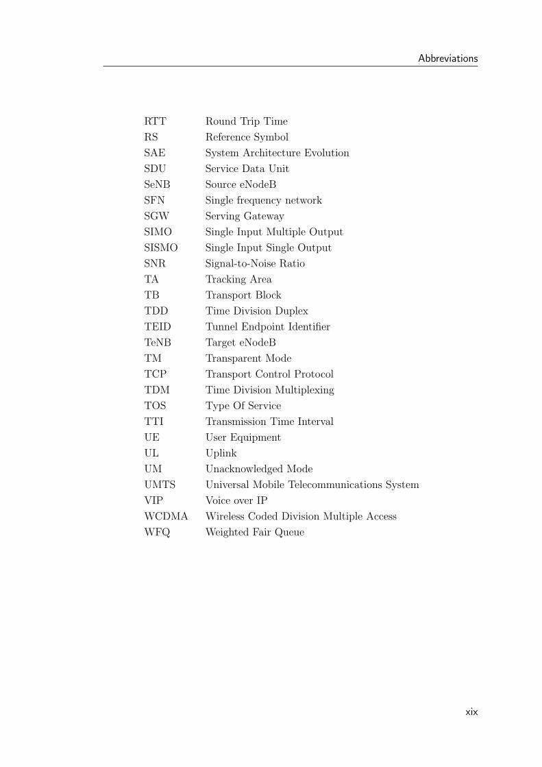
RTT Round Trip Time

RS Reference Symbol

SAE System Architecture Evolution

SDU Service Data Unit

SeNB Source eNodeB

SFN Single frequency network

SGW Serving Gateway

SIMO Single Input Multiple Output

SISMO Single Input Single Output

SNR Signal-to-Noise Ratio

TA Tracking Area

TB Transport Block

TDD Time Division Duplex

TEID Tunnel Endpoint Identifier

TeNB Target eNodeB

TM Transparent Mode

TCP Transport Control Protocol

TDM Time Division Multiplexing

TOS Type Of Service

TTI Transmission Time Interval

UE User Equipment

UL Uplink

UM Unacknowledged Mode

UMTS Universal Mobile Telecommunications System

VIP Voice over IP

WCDMA Wireless Coded Division Multiple Access

WFQ Weighted Fair Queue

xix

Chapter 1

Background

In this chapter we describe the key aspects of LTE. The chapter is then con-

cluded with a detailed description of the handover mechanism of LTE.

1.1 LTE (Long Term Evolution)

The recent increase of mobile data usage and the emergence of new applica-

tions, such as Multimedia Online Gaming (MMOG), mobile TV, Web 2.0, stream-

ing contents, have motivated the 3rd Generation Partnership Project (3GPP) to

work on the Long Term Evolution (LTE). LTE is the latest standard in the mo-

bile network technology tree, which previously implemented the GSM/EDGE

and UMTS/HSxPA network technologies now account for over 85% of all mo-

bile subscribers. LTE will ensure 3GPP’s competitive edge over other cellular

technologies.

LTE, whose radio access is called Evolved UMTS Terrestrial Radio Access

Network (E-UTRAN), is expected to substantially improve end-user through-

puts and sector capacity also to reduce user plane latency, bringing significantly

improved user experience with full mobility. With the emergence of Internet

Protocol (ip) as the protocol of choice for carrying all types of traffic, LTE is

scheduled to provide support for ip-based traffic with end-to-end Quality of ser-

3

1. Background

vice (QoS). Voice traffic will be supported mainly as Voice over ip (VIP) enabling

better integration with other multimedia services. Initial deployments of LTE are

expected by 2010 and commercial availability on a larger scale 1-2 years later.

Unlike High Speed Packet Access (HSPA), which was accommodated within

the Release 99 UMTS architecture, 3GPP is specifying a new Packet Core, the

Evolved Packet Core (EPC) network architecture to support the E-UTRAN

through a reduction in the number of network elements, simpler functionality, im-

proved redundancy but most importantly allowing for connections and handover

to other fixed line and wireless access technologies, giving the service providers

the ability to deliver a seamless mobility experience.

LTE has been set aggressive performance requirements that rely on phys-

ical layer technologies, such as: Orthogonal Frequency Division Multiplexing

(OFDM), Multiple-Input Multiple-Output (MIMO) systems and Smart Anten-

nas to achieve the baseline targets. The main objectives of LTE are to minimize

the system and User Equipment (UE) complexities, allow flexible spectrum de-

ployment in existing or new frequency spectrum and to enable co-existence with

other 3GPP Radio Access Technologies (RATs).

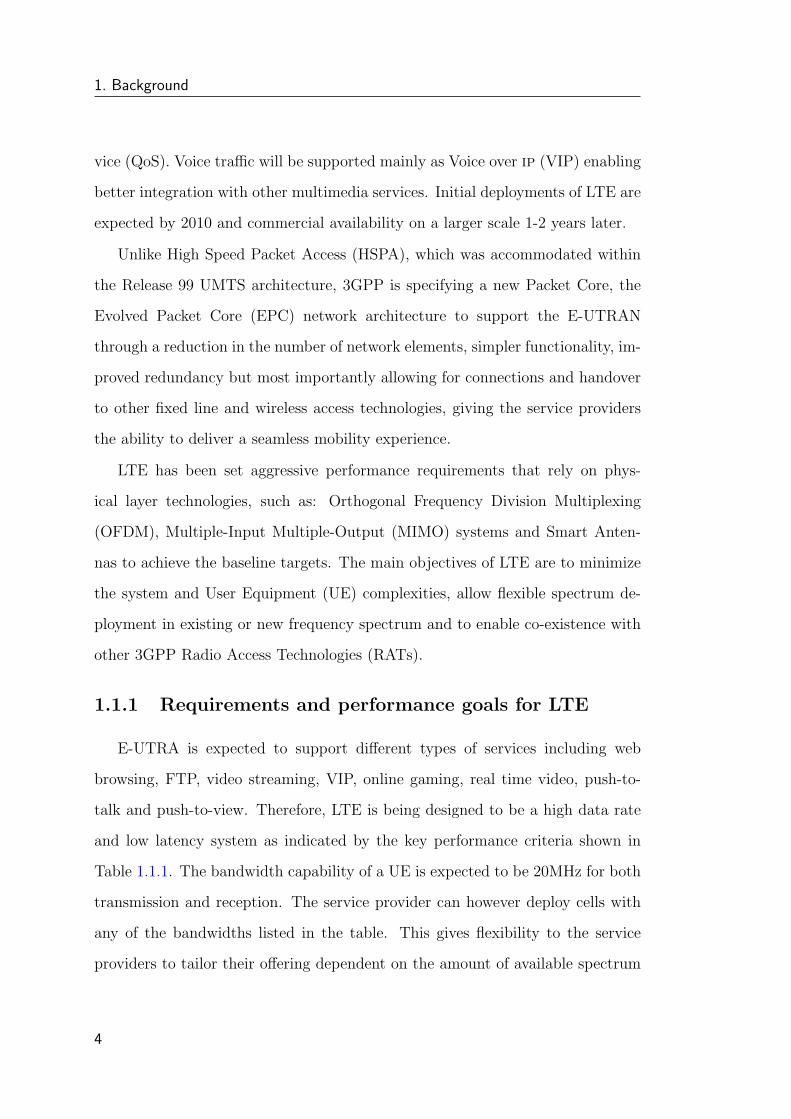
1.1.1 Requirements and performance goals for LTE

E-UTRA is expected to support different types of services including web

browsing, FTP, video streaming, VIP, online gaming, real time video, push-to-

talk and push-to-view. Therefore, LTE is being designed to be a high data rate

and low latency system as indicated by the key performance criteria shown in

Table 1.1.1. The bandwidth capability of a UE is expected to be 20MHz for both

transmission and reception. The service provider can however deploy cells with

any of the bandwidths listed in the table. This gives flexibility to the service

providers to tailor their offering dependent on the amount of available spectrum

4

LTE (Long Term Evolution) 1.1

Metric RequirementPeak data rate DL: 100 Mbps

UL: 50 Mbps(for 20 MHz spectrum)

Mobility support Up to 500 km/h but optimizedfor low speeds from 0 to 15 km/h

Control plane latency < 100 ms (for idle to active)(Transition time to active state)User plane latency < 5 msControl plane capacity > 200 users per cell

(for 5 MHz spectrum)Coverage (Cell sizes) 5-100 km with slight

degradation after 30 kmSpectrum flexibility 1.25, 2.5, 5, 20 MHz

Table 1.1.1. LTE performance goal

or the ability to start with limited spectrum for lower upfront cost and grow the

spectrum for extra capacity.

During 2005 the 3GPP activity on 3G evolution was setting the requirement

for LTE. These are documented in [8] and were divided into seven categories:

• capabilities,

• system performance,

• deployment-related aspects,

• architecture and migration,

• radio resource management,

• complexity,

• general aspects.

5

1. Background

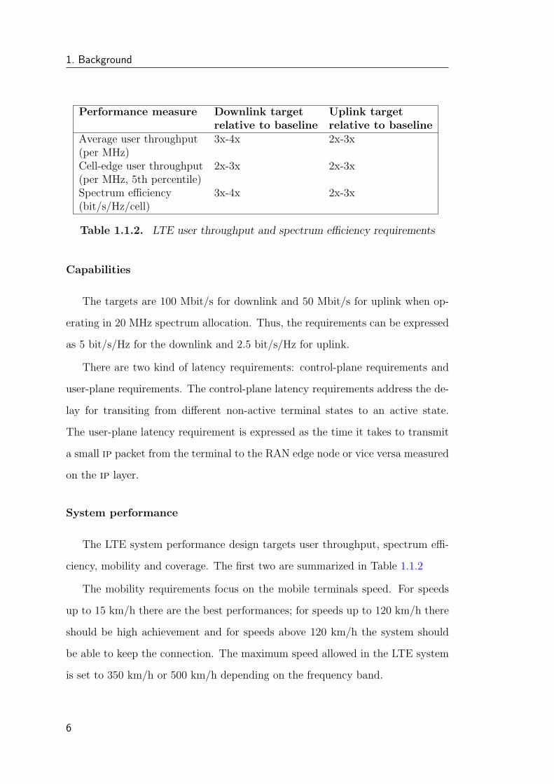
Performance measure Downlink target Uplink targetrelative to baseline relative to baseline

Average user throughput 3x-4x 2x-3x(per MHz)Cell-edge user throughput 2x-3x 2x-3x(per MHz, 5th percentile)Spectrum efficiency 3x-4x 2x-3x(bit/s/Hz/cell)

Table 1.1.2. LTE user throughput and spectrum efficiency requirements

Capabilities

The targets are 100 Mbit/s for downlink and 50 Mbit/s for uplink when op-

erating in 20 MHz spectrum allocation. Thus, the requirements can be expressed

as 5 bit/s/Hz for the downlink and 2.5 bit/s/Hz for uplink.

There are two kind of latency requirements: control-plane requirements and

user-plane requirements. The control-plane latency requirements address the de-

lay for transiting from different non-active terminal states to an active state.

The user-plane latency requirement is expressed as the time it takes to transmit

a small ip packet from the terminal to the RAN edge node or vice versa measured

on the ip layer.

System performance

The LTE system performance design targets user throughput, spectrum effi-

ciency, mobility and coverage. The first two are summarized in Table 1.1.2

The mobility requirements focus on the mobile terminals speed. For speeds

up to 15 km/h there are the best performances; for speeds up to 120 km/h there

should be high achievement and for speeds above 120 km/h the system should

be able to keep the connection. The maximum speed allowed in the LTE system

is set to 350 km/h or 500 km/h depending on the frequency band.

6

LTE (Long Term Evolution) 1.1

Non-real-time (ms) Real-time (ms)relative to baseline relative to baseline

LTE to WCDMA 500 300LTE to GSM 500 300

Table 1.1.3. Interruption time requirements, LTE-GSM and LTE-WCDMA.

The coverage requirements focus on the cell range. The cells up to 5 km of

radius allow non-interference-limited scenarios; for cells range up to 30 km, a

slight performances degradation are tolerated and cell ranges up to 100 km are

not precluded but no performance requirements are stated yet.

Deployment-related aspects

The requirement on the deployment scenario includes both the case when the

LTE system is deployed as a stand-alone system and the case when it is deployed

together with WCDMA/HSPA and/or GSM. For mobile terminals supporting

those technologies, Table 1.1.3 lists the interruption requirements, that is, longest

acceptable interruption in the radio link when moving between the different radio

access technologies, for both real-time and non-real-time services.

The basis for the requirements on spectrum flexibility is the requirement for

LTE to be deployed in existing IMT-2000 frequency bands (coexistence with the

systems that are already deployed in those bands), that is LTE should support

both Frequency Division Duplex (FDD), and Time Division Duplex (TDD) (Fig-

ure 1.1.1).

Architecture and migration

LTE RAN architecture should be packet based (and also support real-time

class traffic), simplify and minimize the interface, support an end-to-end QoS

and designed to minimize the jitter (for example, for tcp/ip traffic type) [8].

7

1. Background

Uplink Downlink

1900 217021102025201019801920

Frequency (MHz)

FDD-Based radio accessTDD-Based radio access

Figure 1.1.1. FDD and TDD operating bands.

Radio resource management

The radio resource management requirements are divided into enhanced sup-

port for end-to-end QoS, efficient support for transmission of higher layers, and

support of load sharing and policy management across different radio access tech-

nologies.

Complexity and general aspects

LTE complexity requirements imply that the number of options should be

minimized with no redundant required features. This has an impact also to

the cost and service related aspects that, specific to the cost, it is desirable to

minimize it maintaining the desired performance.

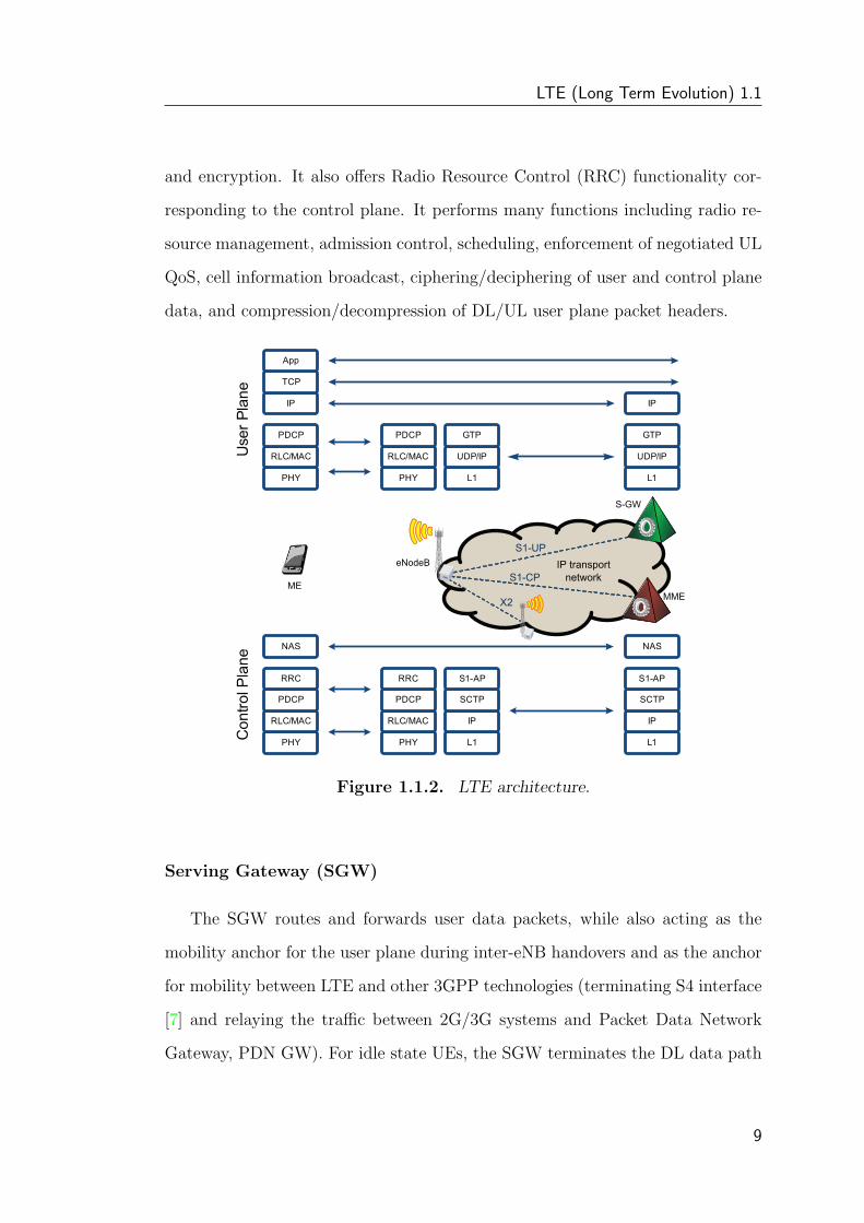
1.1.2 System architecture description

The architecture consists of the following functional elements:

Evolved Radio Access Network (RAN)

The evolved RAN for LTE is composed of a single node, i.e., the eNodeB (eNB)

that interfaces with the UE. The eNB hosts the PHYsical (PHY), Medium Access

Control (MAC), Radio Link Control (RLC), and Packet Data Control Protocol

(PDCP) layers that include the functionality of user-plane header-compression

8

LTE (Long Term Evolution) 1.1

and encryption. It also offers Radio Resource Control (RRC) functionality cor-

responding to the control plane. It performs many functions including radio re-

source management, admission control, scheduling, enforcement of negotiated UL

QoS, cell information broadcast, ciphering/deciphering of user and control plane

data, and compression/decompression of DL/UL user plane packet headers.

IP transportnetwork

S1-UP

S1-CP

X2

IP transportnetwork

S1-UP

S1-CP

X2

PHY

RLC/MAC

PDCP

IP

TCP

App

PHY

RLC/MAC

PDCP

L1

UDP/IP

GTP

L1

UDP/IP

GTP

IP

Use

r Pla

ne

PHY

RLC/MAC

PDCP

RRC

NAS

PHY

RLC/MAC

PDCP

RRC

L1

IP

SCTP

S1-AP

NAS

L1

IP

SCTP

S1-AP

Con

trol P

lane

ME

eNodeB

MME

S-GW

Figure 1.1.2. LTE architecture.

Serving Gateway (SGW)

The SGW routes and forwards user data packets, while also acting as the

mobility anchor for the user plane during inter-eNB handovers and as the anchor

for mobility between LTE and other 3GPP technologies (terminating S4 interface

[7] and relaying the traffic between 2G/3G systems and Packet Data Network

Gateway, PDN GW). For idle state UEs, the SGW terminates the DL data path

9

1. Background

and triggers paging when DL data arrives for the UE. It manages and stores

UE contexts, e.g. parameters of the ip bearer service, network internal routing

information. It also performs replication of the user traffic in case of lawful

interception.

Mobility Management Entity (MME)

The MME is the key control-node for the LTE access network. It is responsible

for idle mode UE tracking and paging procedure including retransmissions. It

is involved in the bearer activation/deactivation process and is also responsible

for choosing the SGW for a UE at the initial attach and at the time of intra-

LTE handover involving Core Network (CN) node relocation. It is responsible

for authenticating the user (by interacting with the Home Subscriber Server,

HSS). The Non-Access Stratum (NAS) signaling terminates at the MME and it

is also responsible for generation and allocation of temporary identities to UEs.

It checks the authorization of the UE to camp on the service provider’s Public

Land Mobile Network (PLMN) and enforces UE roaming restrictions. The MME

is the termination point in the network for ciphering/integrity protection for

NAS signaling and handles the security key management. Lawful interception

of signaling is also supported by the MME. The MME also provides the control

plane function for mobility between LTE and 2G/3G access networks with the

S3 interface terminating at the MME from the SGSN. The MME also terminates

the S6a interface towards the home HSS for roaming UEs.

1.1.3 Key Features

EPS to EPC

A key feature of the EPS is the separation of the network entity that performs

control-plane functionality (MME) from the network entity that performs bearer-

10

LTE (Long Term Evolution) 1.1

plane functionality (SGW) with a well defined open interface between them (S11).

Since E-UTRAN will provide higher bandwidth to enable new services as well

as to improve existing ones, separation of MME from SGW implies that SGW

can be based on a platform optimized for high bandwidth packet processing,

where as the MME is based on a platform optimized for signaling transactions.

This enables selection of more cost-effective platforms for, as well as independent

scaling, of each of these two elements. Service providers can also choose optimized

topological locations of SGWs within the network independent of the locations of

MMEs in order to optimize bandwidth, reduce latencies and avoid concentrated

points of failure.

S1-flex Mechanism

The S1-flex concept provides support for network redundancy and load sharing

of traffic across network elements in the CN, the MME and the SGW, by creating

pools of MMEs and SGWs and allowing each eNB to be connected to multiple

MMEs and SGWs in a pool.

1.1.4 Network Sharing

The LTE architecture enables service providers to reduce the cost of owning

and operating the network by allowing the service providers to have separate CN

(MME, SGW, PDN GW) while the E-UTRAN (eNBs) is jointly shared by them.

This is enabled by the S1-flex mechanism by enabling each eNB to be connected

to multiple CN entities. When a UE attaches to the network, it is connected to

the appropriate CN entities based on the identity of the service provider sent by

the UE.

In this section, we describe the functions of the different protocol layers and

their location in the LTE architecture. In Figure 1.1.2, the NAS protocol, which

11

1. Background

runs between the MME and the UE, is used for control-purposes such as network

attach, authentication, setting up of bearers, and mobility management. All NAS

messages are ciphered and integrity protected by the MME and UE. The RRC

layer in the eNB makes handover decisions based on neighbor cell measurements

sent by the UE, pages for the UEs over the air, broadcasts system information,

controls UE measurement reporting such as the periodicity of Channel Quality

Information (CQI) reports and allocates cell-level temporary identifiers to active

UEs. It also executes transfer of UE context from the Source eNB to the Target

eNB during handover, and does integrity protection of RRC messages. The RRC

layer is responsible for the setting up and maintenance of radio bearers.

In the user-plane, the PDCP layer is responsible for compression/decompres-

sion the headers of user plane ip packets using Robust Header Compression

(ROHC) to enable efficient use of air interface bandwidth. This layer also per-

forms ciphering of both user plane and control plane data. Because the NAS

messages are carried in RRC, they are effectively double ciphered and integrity

protected, once at the MME and again at the eNB.

The RLC layer is used to format and transport traffic between the UE and the

eNB. RLC provides three different reliability modes for data transport: Acknowl-

edged Mode (AM), Unacknowledged Mode (UM), or Transparent Mode (TM).

The UM mode is suitable for transport of Real Time (RT) services because such

services are delay sensitive and cannot wait for retransmissions. The AM mode,

on the other hand, is appropriate for non-RT (NRT) services such as file down-

loads. The TM mode is used when the PDU sizes are known a priori such as for

broadcasting system information. The RLC layer also provides in-sequence de-

livery of Service Data Units (SDUs) to the upper layers and eliminates duplicate

SDUs from being delivered to the upper layers. It may also segment the SDUs

depending on the radio conditions.

12

LTE (Long Term Evolution) 1.1

Furthermore, there are two levels of re-transmissions for providing reliability,

namely, the Hybrid Automatic Repeat reQuest (HARQ) at the MAC layer and

outer ARQ at the RLC layer. The outer ARQ is required to handle residual errors

that are not corrected by HARQ, that is kept simple by the use of a single bit

error-feedback mechanism. An N-process stop-and-wait HARQ is employed that

has asynchronous re-transmissions in the DL and synchronous re-transmissions

in the UL. Synchronous HARQ means that the re-transmissions of HARQ blocks

occur at pre-defined periodic intervals, hence, no explicit signaling is required to

indicate to the receiver the retransmission schedule. Asynchronous HARQ offers

the flexibility of scheduling re-transmissions based on air interface conditions.

The Figure 1.1.3 show the structure of layer 2 for DL. The PDCP, RLC and

MAC layers together constitute layer 2.

ROCH

Security

Segm.ARQ

Scheduling / Priority Handling

ROCH

Security

Segm.

ARQ

ROCH

Security

Segm.

ARQ

ROCH

Security

Segm.

ARQ BCCH PCCH

Multiplexing UE1

HARQ

Multiplexing UEn

HARQ

Radio Bearers

Logical Channels

Transport Channels

MAC

RLC

PDCP

Figure 1.1.3. Layer 2 structure for Downlink.

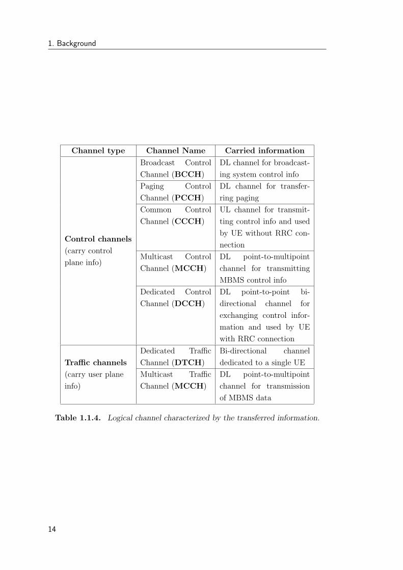
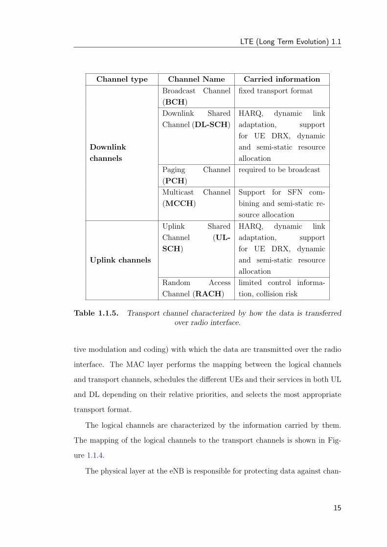
In LTE, there is significant effort to simplify the number and mappings of

logical and transport channels. The different logical and transport channels in

LTE are illustrated in Table 1.1.4 and Table 1.1.5, respectively.

The transport channels are distinguished by the characteristics (e.g. adap-

13

1. Background

Channel type Channel Name Carried information

Control channels

(carry control

plane info)

Broadcast Control

Channel (BCCH)

DL channel for broadcast-

ing system control info

Paging Control

Channel (PCCH)

DL channel for transfer-

ring paging

Common Control

Channel (CCCH)

UL channel for transmit-

ting control info and used

by UE without RRC con-

nection

Multicast Control

Channel (MCCH)

DL point-to-multipoint

channel for transmitting

MBMS control info

Dedicated Control

Channel (DCCH)

DL point-to-point bi-

directional channel for

exchanging control infor-

mation and used by UE

with RRC connection

Traffic channels

(carry user plane

info)

Dedicated Traffic

Channel (DTCH)

Bi-directional channel

dedicated to a single UE

Multicast Traffic

Channel (MCCH)

DL point-to-multipoint

channel for transmission

of MBMS data

Table 1.1.4. Logical channel characterized by the transferred information.

14

LTE (Long Term Evolution) 1.1

Channel type Channel Name Carried information

Downlink

channels

Broadcast Channel

(BCH)

fixed transport format

Downlink Shared

Channel (DL-SCH)

HARQ, dynamic link

adaptation, support

for UE DRX, dynamic

and semi-static resource

allocation

Paging Channel

(PCH)

required to be broadcast

Multicast Channel

(MCCH)

Support for SFN com-

bining and semi-static re-

source allocation

Uplink channels

Uplink Shared

Channel (UL-

SCH)

HARQ, dynamic link

adaptation, support

for UE DRX, dynamic

and semi-static resource

allocation

Random Access

Channel (RACH)

limited control informa-

tion, collision risk

Table 1.1.5. Transport channel characterized by how the data is transferredover radio interface.

tive modulation and coding) with which the data are transmitted over the radio

interface. The MAC layer performs the mapping between the logical channels

and transport channels, schedules the different UEs and their services in both UL

and DL depending on their relative priorities, and selects the most appropriate

transport format.

The logical channels are characterized by the information carried by them.

The mapping of the logical channels to the transport channels is shown in Fig-

ure 1.1.4.

The physical layer at the eNB is responsible for protecting data against chan-

15

1. Background

MTCH MCCH

Logical Channels

Transport Channels

BCCH PCCHDTCH DCCH

DL-SCHUL-SCH BCH PCH MCH

Downlink onlyDownlink or uplink

Figure 1.1.4. Example of mapping of logical channels to transport channels.

nel errors using adaptive modulation and coding (AMC) schemes based on chan-

nel conditions. It also maintains frequency and time synchronization and per-

forms RF processing including modulation and demodulation. In addition, it

processes measurement reports from the UE such as CQI and provides indica-

tions to the upper layers.

The minimum unit of scheduling is a time-frequency block corresponding to

one sub-frame (1 ms) and 12 sub-carriers. The scheduling is not done at a sub-

carrier granularity in order to limit the control signaling. QPSK, 16QAM and

64QAM will be the DL and UL modulation schemes in E-UTRA. For UL, 64-QAM

is optional at the UE. Each radio frame is 10ms long containing 10 sub-frames

with each sub-frame capable of carrying 14 OFDM symbols. For more details on

these access schemes, refer to [4].

Multiple antennas at the UE are supported with the 2 receive and 1 transmit

antenna configuration being mandatory. MIMO (multiple input multiple output)

is also supported at the eNB with two transmit antennas being the baseline

configuration. Orthogonal Frequency Division Multiple Access (OFDMA) with

a sub-carrier spacing of 15 kHz and Single Carrier Frequency Division Multiple

Access (SC-FDMA) have been chosen as the transmission schemes for the DL

and UL, respectively.

16

Mobility management 1.2

1.2 Mobility management

LTE_DETACHED LTE_ACTIVE LTE_IDLE

• No IP address

• Position not known

• IP address assigned

• Position partially known

• DL DRX period

• IP address assigned

• Connected to known cell

Power-Up

OUT_OF_SINK IN_SINK

• DL reception possible

• No UL transmission

• DL reception possible

• UL transmission possible

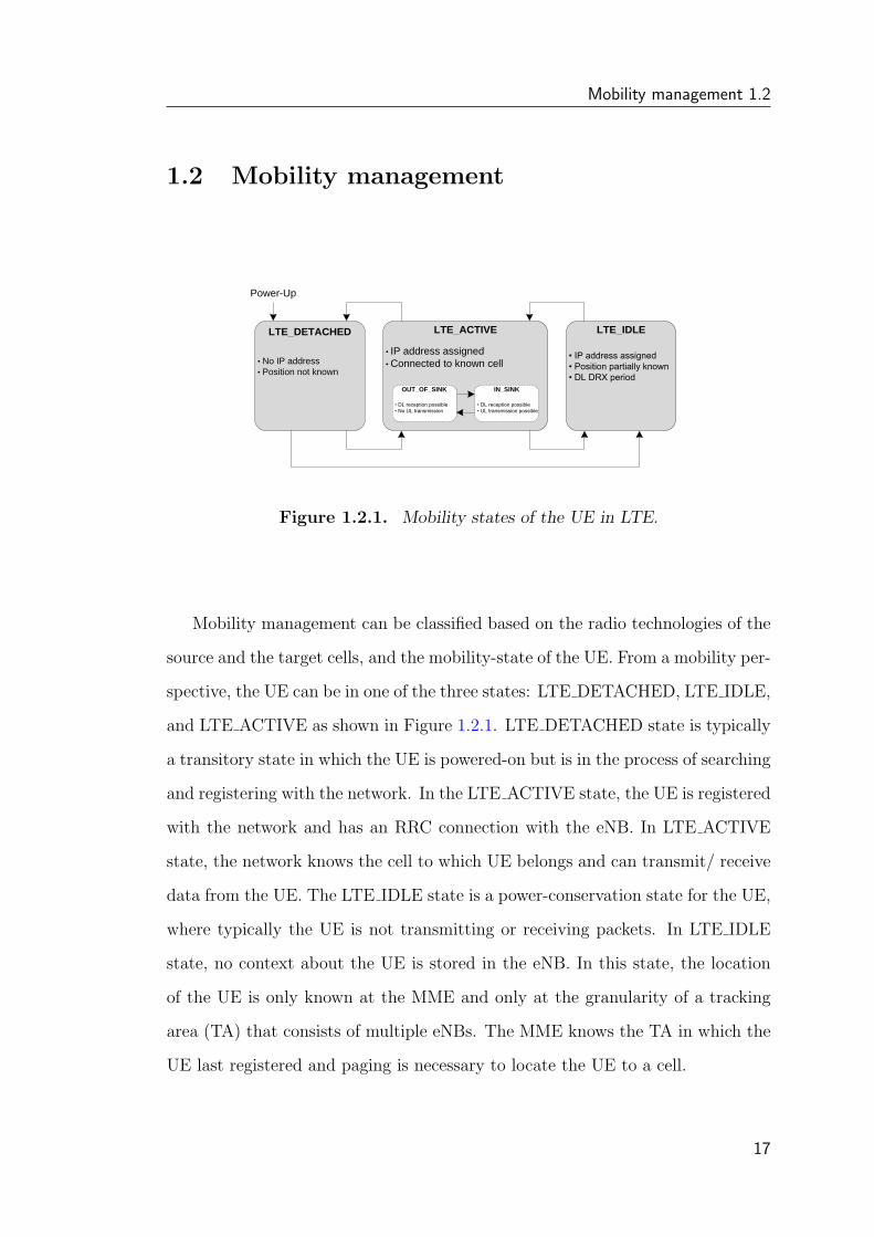
Figure 1.2.1. Mobility states of the UE in LTE.

Mobility management can be classified based on the radio technologies of the

source and the target cells, and the mobility-state of the UE. From a mobility per-

spective, the UE can be in one of the three states: LTE DETACHED, LTE IDLE,

and LTE ACTIVE as shown in Figure 1.2.1. LTE DETACHED state is typically

a transitory state in which the UE is powered-on but is in the process of searching

and registering with the network. In the LTE ACTIVE state, the UE is registered

with the network and has an RRC connection with the eNB. In LTE ACTIVE

state, the network knows the cell to which UE belongs and can transmit/ receive

data from the UE. The LTE IDLE state is a power-conservation state for the UE,

where typically the UE is not transmitting or receiving packets. In LTE IDLE

state, no context about the UE is stored in the eNB. In this state, the location

of the UE is only known at the MME and only at the granularity of a tracking

area (TA) that consists of multiple eNBs. The MME knows the TA in which the

UE last registered and paging is necessary to locate the UE to a cell.

17

1. Background

Transmission BW (MHz) 1.4 3 5 10 15 20Sub-frame duration 1.0 msSub-carrier spacing 15KHzSampling frequency (MHz) 1.92 3.84 7.68 15.36 23.04 30.72FFT size 128 256 512 1024 1536 2048Number of occupied sub-carriers 72 180 300 600 900 1200

CP length (µs)Normal 4.69×6, 5.21×1

Extended 16.6

Table 1.3.6. E-UTRA Numerology

1.3 LTE Technologies

1.3.1 OFDM

In the downlink, OFDM is selected to meet efficiently E-UTRA performance

requirements. With OFDM, it is straightforward to exploit frequency selectiv-

ity of the multi-path channel with low complexity receivers. This allows fre-

quency selective in addition to frequency diverse scheduling and one cell reuse of

available bandwidth. Furthermore, due to its frequency domain nature, OFDM

enables flexible bandwidth operation with low complexity. Smart antenna tech-

nologies are also easier to support with OFDM, since each sub-carrier becomes

flat faded and the antenna weights can be optimized on a per sub-carrier (or

block of sub-carriers) basis. In addition, OFDM enables broadcast services on

a synchronized Single Frequency Network (SFN) with appropriate cyclic prefix

design. This allows broadcast signals from different cells to combine over the air,

thus significantly increasing the received signal power and supportable data rates

for broadcast services.

To provide great operational flexibility, E-UTRA physical layer specifications

are bandwidth agnostic and designed to accommodate up to 20 MHz system

bandwidth. Table 1.3.6 provides the downlink sub-frame numerology for different

spectrum allocations. Sub-frames with one of two cyclic prefix (CP) durations

18

LTE Technologies 1.3

may be time-domain multiplexed, with the shorter designed for unicast trans-

mission and the longer designed for larger cells or broadcast SFN transmission.

The useful symbol duration is constant across all bandwidths. The 15 kHz sub-

carrier spacing is large enough to avoid degradation from phase noise and Doppler

(250km/h at 2.6 GHz) with 64QAM modulation.

The downlink reference signal structure for channel estimation, CQI measure-

ment, and cell search/acquisition is shown in Figure 1.3.1. Reference symbols

(RS) are located in the 1st OFDM symbol (1st RS) and 3rd to last OFDM symbol

(2nd RS) of every slot. For FDD, it may be possible to reduce overhead by not

transmitting the 2nd RS for at least low to medium speeds, since adjacent sub-

frames can often be used to improve channel estimation performance. This dual

TDM (or TDM) structure has similar performance to a scattered structure in 0.5

ms sub-frames, and an advantage in that low complexity channel estimation (in-

terpolation) is supported as well as other excellent performance low-complexity

techniques, such as IFFT-based channel estimators. To provide orthogonal sig-

nals for multi-antenna implementation, FDM is used for different TX antennas

of the same cell, and CDM is used for different cells.

1.3.2 Multiple antenna techniques

Central to LTE is the concept of multiple antenna techniques - often loosely

referred to as MIMO - which take advantage of spatial diversity in the radio

channel. Multiple antenna techniques are of three main types: diversity, MIMO,

and beamforming. These techniques are used to improve signal robustness and

to increase system capacity and single-user data rates. Each technique has its

own performance benefits and costs.

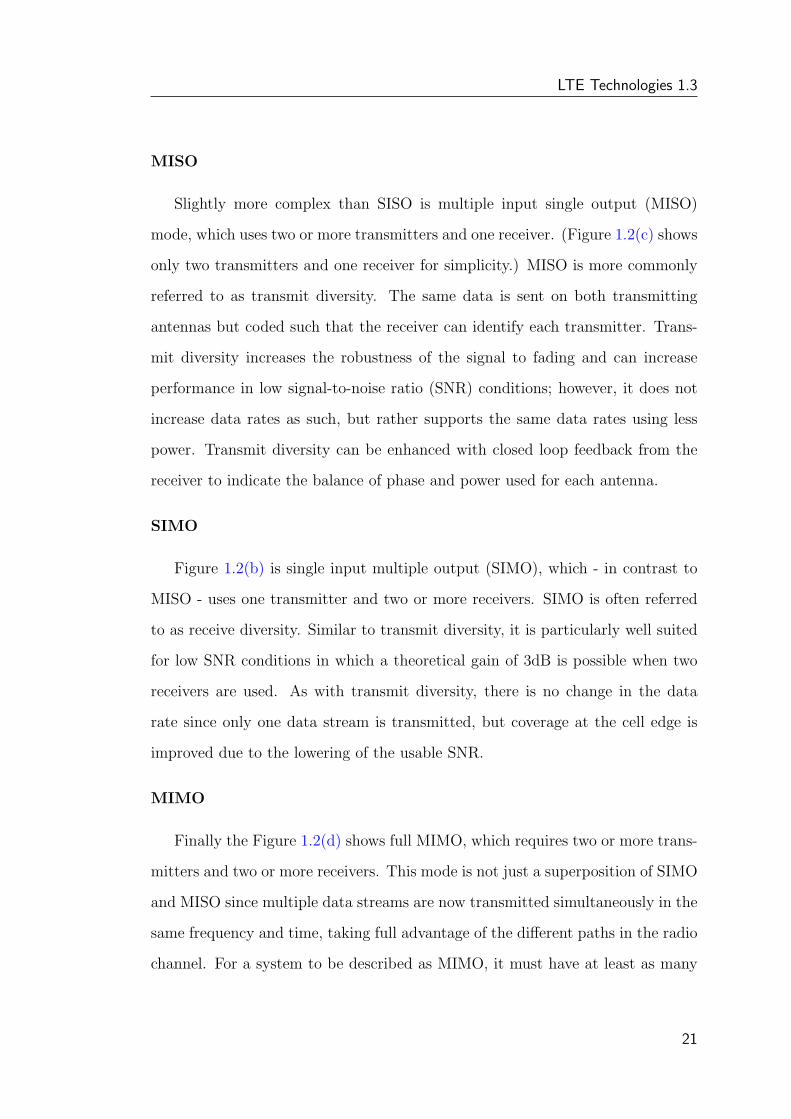
Figure 1.3.2 illustrates the range of possible antenna techniques from the

simplest to the most complex, indicating how the radio channel is accessed by

19

1. Background

R0

R0

R0

R0

R0

R0

R0

R0

Freq

uenc

y

Slot Slot

l=0 l=0l=6 l=6

(a) Antenna port 0.

R1

R1

R1

R1

R1

R1

R1

R1

Freq

uenc

y

Slot Slot

l=0 l=0l=6 l=6

(b) Antenna port 1.

Figure 1.3.1. Downlink reference signal structure - normal cyclic prefix, twotransmit antennas

the system’s transmitters and receivers.

Transmit antennas

Receive antennas The radio channel

(a) SISO system.

Transmit antennas

Receive antennas The radio channel

(b) SIMO system.

(c) MISO system. (d) MIMO system.

Figure 1.3.2. Radio channel access modes

SISO

The most basic radio channel access mode is single input single output (SISO)

in which, only one transmit antenna and one receive antenna are used. This is

the form of communication that has been the default since radio began and is

the baseline to which all the multiple antenna techniques are compared.

20

LTE Technologies 1.3

MISO

Slightly more complex than SISO is multiple input single output (MISO)

mode, which uses two or more transmitters and one receiver. (Figure 1.2(c) shows

only two transmitters and one receiver for simplicity.) MISO is more commonly

referred to as transmit diversity. The same data is sent on both transmitting

antennas but coded such that the receiver can identify each transmitter. Trans-

mit diversity increases the robustness of the signal to fading and can increase

performance in low signal-to-noise ratio (SNR) conditions; however, it does not

increase data rates as such, but rather supports the same data rates using less

power. Transmit diversity can be enhanced with closed loop feedback from the

receiver to indicate the balance of phase and power used for each antenna.

SIMO

Figure 1.2(b) is single input multiple output (SIMO), which - in contrast to

MISO - uses one transmitter and two or more receivers. SIMO is often referred

to as receive diversity. Similar to transmit diversity, it is particularly well suited

for low SNR conditions in which a theoretical gain of 3dB is possible when two

receivers are used. As with transmit diversity, there is no change in the data

rate since only one data stream is transmitted, but coverage at the cell edge is

improved due to the lowering of the usable SNR.

MIMO

Finally the Figure 1.2(d) shows full MIMO, which requires two or more trans-

mitters and two or more receivers. This mode is not just a superposition of SIMO

and MISO since multiple data streams are now transmitted simultaneously in the

same frequency and time, taking full advantage of the different paths in the radio

channel. For a system to be described as MIMO, it must have at least as many

21

1. Background

receivers as there are transmit streams. The number of transmit streams should

not be confused with the number of transmit antennas. Consider the Tx diver-

sity (MISO) case in which two transmitters are present but only one data stream.

Adding receive diversity (SIMO) does not turn this into MIMO, even though there

are now two Tx and two Rx antennas involved. SIMO + MISO 6= MIMO. It is

always possible to have more transmitters than data streams but not the other

way around. If N data streams are transmitted from less than N antennas, the

data cannot be fully descrambled by any number of receivers since overlapping

streams without the addition of spatial diversity just creates interference. How-

ever, by spatially separating N streams across at least N antennas, N receivers

will be able to fully reconstruct the original data streams provided the crosstalk

and noise in the radio channel are low enough.

One other crucial factor for MIMO operation is that the transmissions from

each antenna must be uniquely identifiable so that each receiver can determine

what combination of transmissions has been received. This identification is usu-

ally done with pilot signals, which use orthogonal patterns for each antenna.

The spatial diversity of the radio channel means that MIMO has the potential

to increase the data rate. The most basic form of MIMO assigns one data stream

to each antenna.

In this form, one data stream is uniquely assigned to one antenna. The channel

then mixes up the two transmissions such that at the receivers, each antenna

sees a combination of each stream. Decoding the received signals is a clever

process in which the receivers, by analyzing the patterns that uniquely identify

each transmitter, determine what combination of each transmit stream is present.

The application of an inverse filter and summing of the received streams recreates

the original data.

The theoretical gains from MIMO are a function of the number of transmit and

22

LTE Technologies 1.3

receive antennas, the radio propagation conditions, the ability of the transmitter

to adapt to the changing conditions, and the SNR. The ideal case is one in which

the paths in the radio channel are completely uncorrelated, almost as if separate,

physically cabled connections with no crosstalk existed between the transmitters

and receivers. Such conditions are almost impossible to achieve in free space, and

with the potential for so many variables, it is neither helpful nor possible to quote

MIMO gains without stating the conditions. The upper limit of MIMO gain in

ideal conditions is more easily defined, and for a 2x2 system with two simultaneous

data streams a doubling of capacity and data rate is possible. MIMO works best

in high SNR conditions with minimal line of sight.

Beamforming

Beamforming uses the same signal processing and antenna techniques as

MIMO but rather than exploit de-correlation in the radio path, beamforming

aims to exploit correlation so that the radiation pattern from the transmitter is

directed towards the receiver. This is done by applying small time delays to a

calibrated phase array of antennas. The effectiveness of beamforming varies with

the number of antennas. With just two antennas little gain is seen, but with

four antennas the gains are more useful. Obtaining the initial antenna timing

calibration and maintaining it in the field are challenge.

Combining beamforming and MIMO

The most advanced form of multiple antenna techniques is probably the com-

bination of beamforming with MIMO. In this mode MIMO techniques could be

used on sets of antennas, each of which comprises a beamforming array. Given

that beamforming with only two antennas has limited gains, the advantage of

combining beamforming and MIMO will not be realized unless there are many

23

1. Background

antennas. This limits the practical use of the technique on cost grounds.

1.3.3 Scheduling

Scheduling controls the allocation of the shared resources among the users and

often is jointed to link adaptation; if this happens we have a channel-dependent

scheduling (Figure 1.3.3). In LTE a part of the scheduler is the rate adaptation,

so it determines the data rate to be used for each link.

User #1

User #2

Effective channel variationsseen by the base station

#1 #2 #1 #2 Time

Cha

nnel

qual

ity

(a) Time domain scheduling.

User #1

User #2

Effective channel variationsseen by the base station

#1 #2 #1 #2 Frequency

Cha

nnel

qual

ity

#1 #2

(b) Frequency domain scheduling.

Figure 1.3.3. Channel-dependent scheduling.

LTE has also, in addition to the time domain, access to the frequency domain,

due to the use of OFDM. In other words, scheduling in LTE can take channel

variations into account not only in the time domain, as HSPA, but also in the

frequency domain and this meant that for LTE, scheduling decisions can be taken

as often as once every 1 ms and the granularity in the frequency domain is 180

kHz.

1.4 Handover

In case of a handover the protocol endpoints that are located in the eNodeB

will need to be moved from the Source eNodeB to the Target eNodeB. Then,

it is an option whether the full protocol status of the Source eNodeB is trans-

ferred to the Target eNodeB or the protocols are reinitialized after the handover.

24

Handover 1.4

This raises the question for example, whether the HARQ and ARQ window state

is discarded and reset or transferred during the handover. Since, it would be

overly complex and not always feasible to transfer the whole protocol state, it

is an assumption in LTE that the RLC/MAC protocols are reset after a han-

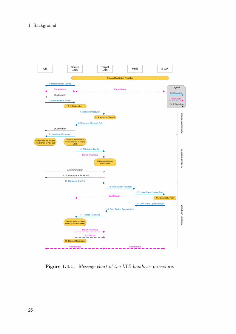
dover. The message sequence diagram of the LTE handover procedure is shown

in Figure 1.4.1.

The figure shows both the control plane messages (black and blue solid arrows)

and the flow of the user plane packets (purple dashed arrows). See also [4] for a

description of the procedure. The UE sends measurement reports to the Source

eNodeB, which may decide on the execution of a handover. The Source eNodeB

requests the preparation of a handover at the Target eNodeB. The Target eNodeB

can perform admission control to check whether the established QoS bearers of

the UE can be accommodated in the target cell.

Next, the Source eNodeB sends the Handover Command to the UE, which

includes all necessary information for the UE to access the target cell. At the

same time the Source eNodeB suspends the RLC/MAC protocols and it may start

to forward the SDUs that have not yet been successfully sent to the UE toward

the Target eNodeB. That is, partially transmitted SDUs at the HARQ/ARQ

layers will be forwarded along with the buffered and not yet transmitted SDUs,

also including all the incoming SDUs from the GW. Whether SDU forwarding is

employed at all by the eNodeB is left as a vendor specific implementation detail.

At the same time, the UE starts to execute the handover to reconnect at

the Target eNodeB. The UE needs to perform a random access procedure on

the RACH (Random Access Channel) in the target cell. The UE also needs to

get uplink time alignment assigned, which means that the eNodeB has to mea-

sure on the uplink transmission of the UE (on the RACH) and determine the

timing advance that the UE has to use for its uplink transmissions in order for

25

1. Background

UE SourceeNB

TargeteNB MME S-GW

0. Area Restriction Provided

1. Measurement Control

Packet Data Packet Data

UL allocation

2. Measurement Report

3. HO decision

4. Handover Request

6. Handover Request Ack

5. Admission Control

DL allocation

7. Handover Command

Detach from old cell andsynchronize to new cell

Deliver buffered and intransit packets to target

eNB

8. SN Status Tranfer

Data Forwarding

Buffer packets fromSource eNB

9. Syncronization

10. UL Allocation + TA for UE

11. Handover Confirm

12. Path Switch Request

13. User Plane Update Req

14. Switch DL Path

15. User Plane Update Reply

16. Path Switch Request Ack

17. Relase Resource

End Marker

Flush DL buffer, continuedelivering in transit packets

Data Forwarding

End Marker

18. Relase Resources

Packet Data Packet Data

Han

dove

rPre

para

tion

Han

dove

rExe

cutio

nH

ando

verC

ompl

etio

n

L3 Signaling

User Data

L1/L2 Signaling

Legend

Figure 1.4.1. Message chart of the LTE handover procedure.

26

Handover 1.4

the received signals from multiple UEs arrive time synchronized at the eNodeB.

Note that in OFDM [5] it is important to keep an accurate time synchronization

between carriers in order to maintain orthogonality. The UE also needs to get

UL/DL resources scheduled in order to be able to commence user data trans-

mission. These L1/L2 access procedures, i.e., the radio interruption time at a

handover, are estimated to take approximately 30 ms [6].

Next, the UE sends the Handover Complete message in the target cell, which

is used by the Target eNodeB to verify that it is the right UE that is accessing the

target cell. At that point the Target eNodeB can start sending DL data to the

UE. The Target eNodeB sends the path switch command to the GW and finally,

it triggers the release of resources at the Source eNodeB. Note that there can be

a time interval after the path switch when packets both on the direct path and

also on the forwarding path arrive in parallel at the Target eNodeB. This may

give rise to the problem of out of order packet delivery as explained below.

In fact, during the handover procedure there is a time interval when packets

on the direct path (GW - Target eNodeB) and packets on the forwarding path

(GW - Source eNodeB - Target eNodeB) may arrive in parallel at the Target

eNodeB. This gives rise to the potential problem of out of order packet delivery

to the UE, since packets on the direct path typically travel a shorter distance and

arrive earlier to the Target eNodeB than packets on the forwarding path. Note

that out of order packet arrivals may have a bad impact on tcp performance and

may result in a loss of system utilization. When three or more packets arrive out

of order, it results in duplicate acks received at the tcp sender, which will react

with a retransmission and congestion window halving.

The problem mentioned above has been analyzed and solved in [6], where the

solution consists in a packet reordering feature inside the TeNB to avoid the out

of order delivering.

27

1. Background

1.5 Summary

In this chapter we have seen that the main objectives of Long Term Evolution

(LTE) are (1) instantaneous peak data rate 100 Mbps in downlink and 50 Mbps

in uplink within a 20 MHz spectrum allocation, the data rate is scalable with

the spectrum allocation; (2) user throughput improved by factor of 2-3 in uplink

and downlink respectively; reduced control-plane latency; (3) user-plane latency

below 5 ms for small ip packet in an unloaded network; (4) improved spectrum

efficiency by factor of 2-3 in uplink and downlink respectively; (5) co-existence

and interworking with legacy standards; (6) reduced cost.

A detailed description of the handover procedure in LTE is given by a message

chart that includes the control plane messages and the flow of the user plane pack-

ets. In the next chapter, we give a description of TCP with particular reference

to LTE.

28

Chapter 2

TCP and LTE

In this chapter we describe the Transmission Control Protocol and his appli-

cation to LTE.

The most commonly used transport layer protocols are tcp and udp. udp[12]

is a connectionless protocol that does not guarantee delivery of data, it does not

make any error check on the payload. It is used in server client type request-reply

situations and in applications where prompt delivery of data is more important

than accurate delivery, like video streaming.

The Transmission Control Protocol (tcp) is one of the core protocols of the

Internet Protocol Suite. tcp is so central that the entire suite is often referred

to as “tcp/ip”. Whereas ip handles lower-level transmissions from computer

to computer as a message makes its way across the Internet, tcp operates at a

higher level, concerned only with the two end systems, for example a Web browser

and a Web server.

tcp/ip manages the end-to-end reliability in the Transport layer. The topic

of this section is the Transmission Control Protocol (tcp) which is the predom-

inant transport protocol of the Internet today carrying more than 80% of the

total traffic volume. tcp is used by a range of different applications such as

web-traffic (www), file transfer (ftp, ssh), e-mail and even streaming media ap-

29

2. TCP and LTE

plication with “almost real-time” constraints such as, e.g., Internet radio. Among

its management tasks, tcp controls message size, the rate at which messages are

exchanged, and network traffic congestion.

2.1 Importance of TCP

tcp provides a communication service at an intermediate level between an

application program and the Internet Protocol (ip). That is, when an application

program desires to send a large chunk of data across the Internet using ip, instead

of breaking the data into ip-sized pieces and issuing a series of ip requests, the

software can issue a single request to tcp and let tcp handle the ip details.

ip works by exchanging pieces of information called packets. A packet is a

sequence of bytes and consists of a header followed by a body. The header de-

scribes the packet’s destination and, optionally, the routers to use for forwarding

- generally in the right direction - until it arrives at its final destination. The

body contains data which ip is transmitting. When ip is transmitting data on

behalf of tcp, the content of the ip packet body is tcp payload.

Due to network congestion, traffic load balancing, or other unpredictable net-

work behavior, ip packets can be lost or delivered out of order. tcp detects these

problems, requests retransmission of lost packets, rearranges out-of-order packets,

and even helps minimize network congestion to reduce the occurrence of other

problems. Once the tcp receiver has finally reassembled a perfect copy of data

originally transmitted, it passes that datagram to the application program. Thus,

tcp abstracts the application’s communication from the underlying networking

details.

30

TCP key features 2.2

2.2 TCP key features

tcp[11] is a reliable transport protocol with connection procedure that pro-

vides a in-sequence data delivering from a sender to a receiver. Some of the

tcp properties may be desired by certain applications.

The tcp reliability is achieved using ARQ mechanism based on positive ac-

knowledgments. tcp protocol provides transparent segmentation and reassembly

of user data and handles both data flow and congestion. tcp packets are cumula-

tively acknowledged when they arrive in sequence; out of sequence packets cause

the generation of duplicate acknowledgments. For each segment transmission, a

retransmission timer is started; retransmission timers are continuously updated

on a weighted average of previous round trip time (rtt) measurements, i.e. the

time it takes from the transmission of a segment until the paired acknowledgment

is received. tcp sender detects a loss either when multiple duplicate acknowl-

edgments (3 is the default value) arrive, this imply that the packet after the last

acknowledged one has been lost, or when a retransmission timeout (RTO) expires.

The RTO value is calculated dynamically based on rtt measurements. Its accu-

racy is critical, delayed timeouts slow down recovery or redundant retransmissions

can occur due to mistakes in the RTO evaluation.

2.2.1 Flow control

For the flow control tcp uses a sliding window mechanism. It limits the

amount of data that can be sent without waiting for acknowledgement (ack)

from the receiver and when the window is constant, this results in the so called

ack-clock.

31

2. TCP and LTE

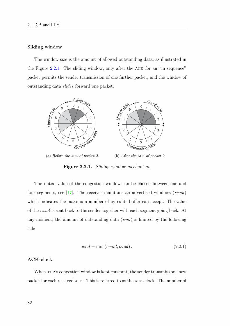
Sliding window

The window size is the amount of allowed outstanding data, as illustrated in

the Figure 2.2.1. The sliding window, only after the ack for an “in sequence”

packet permits the sender transmission of one further packet, and the window of

outstanding data slides forward one packet.

1

2

3

45

6

7

8

90

(a) Before the ack of packet 2.

1

2

3

45

6

7

8

90

(b) After the ack of packet 2.

Figure 2.2.1. Sliding window mechanism.

The initial value of the congestion window can be chosen between one and

four segments, see [17]. The receiver maintains an advertised windows (rwnd)

which indicates the maximum number of bytes its buffer can accept. The value

of the rwnd is sent back to the sender together with each segment going back. At

any moment, the amount of outstanding data (wnd) is limited by the following

rule

wnd = min (rwnd, cwnd) . (2.2.1)

ACK-clock

When tcp’s congestion window is kept constant, the sender transmits one new

packet for each received ack. This is referred to as the ack-clock. The number of

32

TCP Applicability 2.3

packets inside the network (be they data packets or acks) is kept constant. The

ack-clock is based on the idea that by controlling the number of packets inside

the network, we can control the load of the network. The average transmission

rate is one window of data per rtt. In tcp congestion control, the control signal

is the window size, and the actual sending rate is controlled only indirectly by

adjusting the window. This can be seen as a cascaded control system, where

the ack-clock is a fast inner-loop, operating on a per-packet timescale, which is

combined with an outer-loop that adjusts the window size, and operates on an

per-rtt timescale.

2.3 TCP Applicability

tcp is used extensively by many of the Internet’s most popular application

protocols and resulting applications, however, because tcp is optimized for ac-

curate delivery rather than timely delivery, tcp sometimes incurs relatively long

delays (in the order of seconds) while waiting for out-of-order messages or re-

transmissions of lost messages, and it is not particularly suitable for real-time

applications such as Voice over ip. For such applications, protocols like the Real-

time Transport Protocol (rtp) running over the User Datagram Protocol (udp)

are usually recommended instead.

tcp is a reliable stream delivery service that guarantees delivery of a data

stream sent from one host to another without duplication or losing data. Since

packet transfer is not reliable, a technique known as positive acknowledgment

with retransmission is used to guarantee reliability of packet transfers. This

fundamental technique requires the receiver to respond with an acknowledgment

message as it receives the data. The sender keeps a record of each packet it sends,

and waits for acknowledgment before sending the next packet. The sender also

33

2. TCP and LTE

keeps a timer starting from the moment the packet was sent, and retransmits a

packet if the timer expires (rto). The timer is needed in case a packet gets lost

or corrupt.

tcp consists of a set of rules: for the protocol, that are used with the Internet

Protocol, and for the ip, to send data “in a form of message units” between com-

puters over the Internet. At the same time that the ip takes care of handling the

actual delivery of the data, the tcp takes care of keeping track of the individual

units of data “packets” (or more accurately, “segments1”) that a message is di-

vided into for efficient routing through the net. For example, when a html file is

sent from a Web server, the tcp program layer of that server takes the file as a

stream of bytes and divides it into segments, numbers the segments, and then for-

wards them individually to the ip program layer. The ip program layer then turns

each tcp segment into an ip packet by adding a header which includes (among

other things) the destination ip address. Even though every packet has the same

destination ip address, they can get routed differently through the network. When

the client program in your computer gets them, the tcp stack (implementation)

reassembles the individual segments and ensures they are correctly ordered as it

streams them to an application.

Over wireless networks, where losses are mainly caused by mobility and in-

termittent poor channel conditions [14], poor tcp performance is experienced.

Common tcp version misinterpret delays as congestion indications, sometimes

useless retransmissions are experienced and much time is wasted during the slow

start and the congestion avoidance phases. Some solutions have been found by

1tcp accepts data from a data stream, segments it into chunks, and adds a tcp headercreating a tcp segment. The tcp segment is then encapsulated into an IP packet. A tcp seg-ment is “the packet of information that tcp uses to exchange data with its peers.” Note thatthe term tcp packet is now used interchangeably with the term tcp segment, although in theoriginal RFC segment usually referred to the tcp unit of data

34

TCP Applicability 2.3

introducing changes in the tcp paradigm. Westwood tcp for example tries to im-

prove the classic tcp behavior to keep it applicable over both wireless and wired

networks. tcp selective acknowledgments (sack)[16] is proposed to alleviate the

inefficiency of tcp in handling multiple drops in a single data window.

2.3.1 Congestion control

tcp was initially designed to be used in wired networks which has extremely

low transmission losses (BERs lower than 10−10), it assumes that all losses are

due to congestion. Therefore, when tcp detects packet losses, it reacts both

retransmitting the lost packet and reducing the transmission rate. In this way it

allows a reduction of the router queues length. Afterwards, it gradually increases

the transmission rate to probe the network’s capacity.

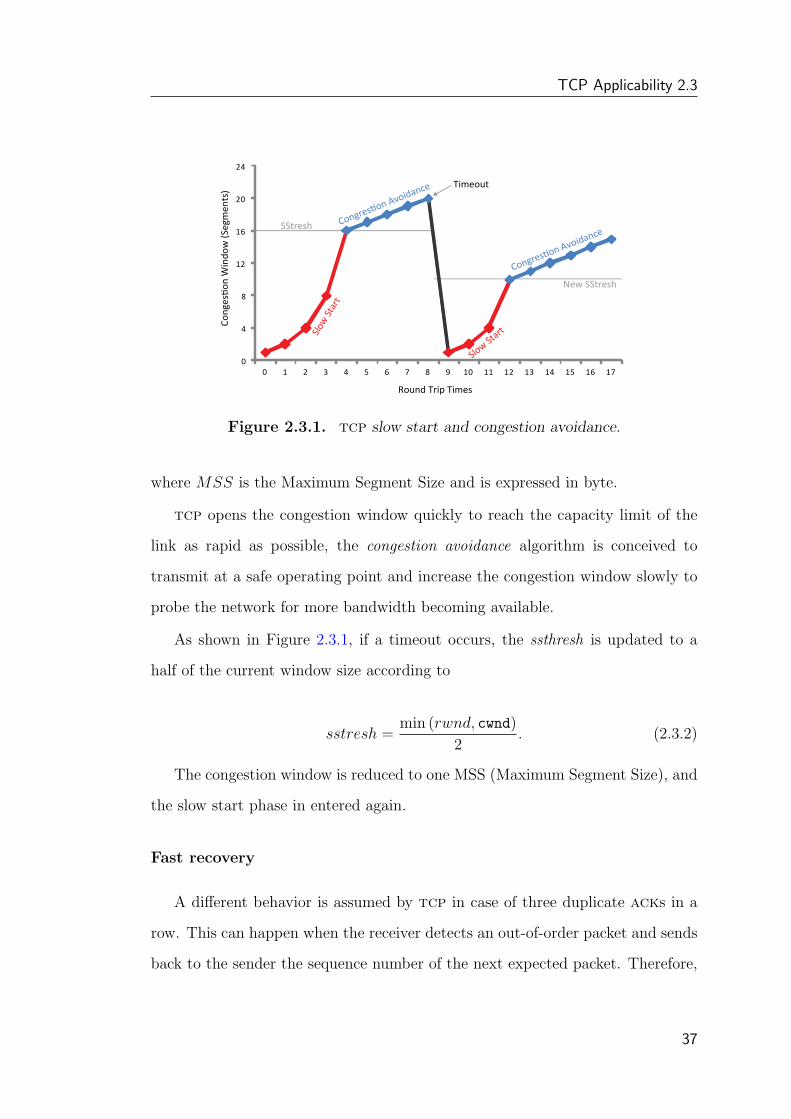
The purpose of slow start and congestion avoidance is to prevent the con-

gestion from occurring varying the transmission rate. For this reason tcp uses

a congestion window (cwnd), which represents the number of segments that the

network might deliver without congestion occurring.

Today all tcp implementations are provided of congestion control algorithm

such slow start, congestion avoidance, fast retransmit and fast recovery[13].

Slow start

In the slow start phase, the congestion window is increased by one segment

for each acknowledgment received. This phase is used both at the beginning of a

new connections and after retransmissions due to RTO expiring. During the slow

start phase cwnd experiences an exponential increase until a timeout occurs or a

threshold value (ssthresh) is reached. In the first case the cwnd will be set to one

packet, instead in the second case, the slow start phase ends and the congestion

avoidance phase starts.

35

2. TCP and LTE

In this state, cwnd is increased by one packet for each non-duplicate ack. The

effect is that for each received ack, two new packets are transmitted. This implies

that the congestion window, and also the sending rate, increases exponentially,

doubling once per rtt.

The motivation for the slow start state is that when a new flow enters the

network, and there is a bottleneck link along the path, then the old flows sharing

that link need some time to react and slow down before there is room for the new

flow to send at full speed.

Congestion avoidance

In the congestion avoidance state, cwnd is increased by one packet per rtt (if

cwnd reaches the maximum value, it stays there). This corresponds to a linear

increase in the sending rate. On timeout, tcp enters the exponential back-off

state2, and on three duplicate acks, it enters the fast recovery state.

The motivation for this congestion avoidance mechanism is that since tcp does

not know the available capacity, it has to probe the network to see at how high

a rate data can get through.

The main difference between slow start and congestion avoidance algorithm is

the way to update the cwnd value (the first it is exponential while for the second

it is linear) as shown in

cwnd =

cwnd + 1, Slow Start ;

cwnd + MSS · MSS

cwnd, Congestion avoidance.

(2.3.1)

2In the exponential back-off mode, once timeout occurred, tcp takes the following actions:(1) The lost packet is retransmitted. (2) The state variables are updated as follow: cwnd isset at 1 packet and ssthresh is set to the value of cwnd/2. (3) The rto value is doubled.The motivation for the exponential back-off mechanism is to avoid congestion collapse due totimeout, that is a sign of severe network congestion.

36

TCP Applicability 2.3

0

4

8

12

16

20

24

0 1 2 3 4 5 6 7 8 9 10 11 12 13 14 15 16 17

Timeout

SStresh

New SStresh

Slow

Sta

rt

Congrestion Avoidance

Congrestion Avoidance

Slow Start

Round Trip Times

Cong

estio

n W

indo

w (S

egm

ents

)

Figure 2.3.1. tcp slow start and congestion avoidance.

where MSS is the Maximum Segment Size and is expressed in byte.

tcp opens the congestion window quickly to reach the capacity limit of the

link as rapid as possible, the congestion avoidance algorithm is conceived to

transmit at a safe operating point and increase the congestion window slowly to

probe the network for more bandwidth becoming available.

As shown in Figure 2.3.1, if a timeout occurs, the ssthresh is updated to a

half of the current window size according to

sstresh =min (rwnd, cwnd)

2. (2.3.2)

The congestion window is reduced to one MSS (Maximum Segment Size), and

the slow start phase in entered again.

Fast recovery

A different behavior is assumed by tcp in case of three duplicate acks in a

row. This can happen when the receiver detects an out-of-order packet and sends

back to the sender the sequence number of the next expected packet. Therefore,

37

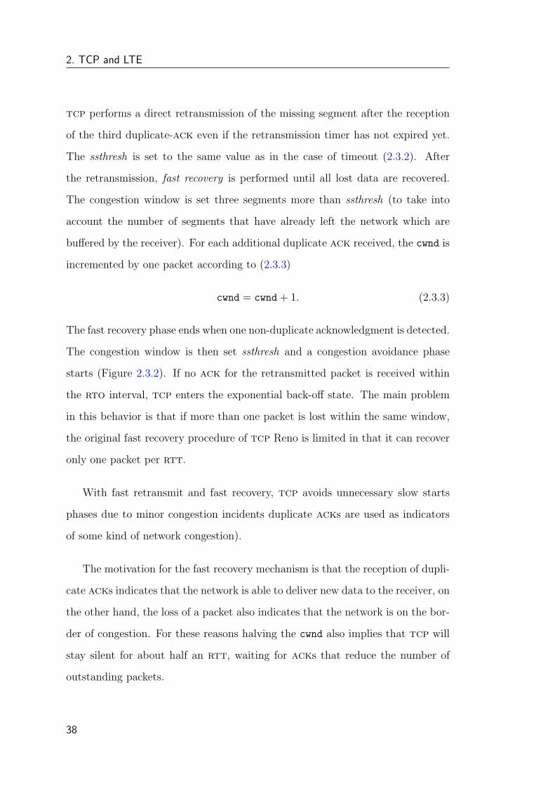
2. TCP and LTE

tcp performs a direct retransmission of the missing segment after the reception

of the third duplicate-ack even if the retransmission timer has not expired yet.

The ssthresh is set to the same value as in the case of timeout (2.3.2). After

the retransmission, fast recovery is performed until all lost data are recovered.

The congestion window is set three segments more than ssthresh (to take into

account the number of segments that have already left the network which are

buffered by the receiver). For each additional duplicate ack received, the cwnd is

incremented by one packet according to (2.3.3)

cwnd = cwnd + 1. (2.3.3)

The fast recovery phase ends when one non-duplicate acknowledgment is detected.

The congestion window is then set ssthresh and a congestion avoidance phase

starts (Figure 2.3.2). If no ack for the retransmitted packet is received within

the rto interval, tcp enters the exponential back-off state. The main problem

in this behavior is that if more than one packet is lost within the same window,

the original fast recovery procedure of tcp Reno is limited in that it can recover

only one packet per rtt.

With fast retransmit and fast recovery, tcp avoids unnecessary slow starts

phases due to minor congestion incidents duplicate acks are used as indicators

of some kind of network congestion).

The motivation for the fast recovery mechanism is that the reception of dupli-

cate acks indicates that the network is able to deliver new data to the receiver, on

the other hand, the loss of a packet also indicates that the network is on the bor-

der of congestion. For these reasons halving the cwnd also implies that tcp will

stay silent for about half an rtt, waiting for acks that reduce the number of

outstanding packets.

38

TCP Applicability 2.3

0

4

8

12

16

20

24

0 1 2 3 4 5 6 7 8 9 10 11 12 13 14 15 16 17

3rd duplicate Ack

SStresh

New SStresh

Slow

Sta

rt

Congrestion Avoidance

Congrestion Avoidance

Round Trip Times

Cong

estio

n W

indo

w (S

egm

ents

)

Fast Recovery

New Ack

(fast retransmit)

Figure 2.3.2. tcp fast retransmit and fast recovery.

2.3.2 Explicit Congestion Notification (ECN)

ECN is an extension to the Internet Protocol and is defined in [19]. ECN

allows end-to-end notification of network congestion without dropping packets.

It is an optional feature and is only used when both endpoints signal that they

want to use it (ECN negotiation occur during the three way handshaking).

Traditionally, tcp/ip networks signal congestion by dropping packets. When

ECN is successfully negotiated, an ECN-aware router may set one bit in the

ip header instead of dropping a packet in order to signal the beginning of conges-

tion. The receiver of the packet echoes the congestion indication to the sender,

which must react as though a packet drop were detected. Obviously this policy

is useful only if it is used in a network where the nodes have an Active Queue

Management (AQM) algorithm.

ECN uses two bits in the ipv4 Type Of Service (TOS) field in the ip header.

These two bits can be used to encode one of the values ECN-unaware transport,

ECN-aware transport or congestion experienced as shown in Figure 2.3.3.

In addition to the two ECN bits in the ip header, tcp uses two flags in the

39

2. TCP and LTE

0 1 2 3 4 5 6 7

Differentiated Service CodePoint ECN

ECT CE

0 0

0 1

1 0

1 1

ECN-unaware

ECN-aware

ECN-aware

Congestion Experienced

Figure 2.3.3. The TOS field in ip header and ECN signaling.

tcp header to signal the sender to reduce the amount of information it sends.

These are the ECN-echo (ECE) and Congestion Window Reduced (CWR) bits

(Figure 2.3.4).

0 1 2 3 4 5 6 7

Header Length Reserved

8 9 10 11 12 13 14 15

CWR ECE URG ACK PSH RST SYN FIN

Figure 2.3.4. Bytes 13 and 14 of the tcp header.

Once the receiver get a tcp segment with the Congestion Experienced code-

point, the tcp receiver sends an acknowledgement with the ECN-echo (ECE)

flag set. The ECN-echo bit indicates congestion to the sender, which reduces its

congestion window as for a packet drop. It then acknowledges the congestion

indication by sending a segment with the Congestion Window Reduced (CWR)

codepoint.

2.4 Evaluation of TCP Performance

tcp performance can be evaluated in different ways depending on the context,

such as the system used and the application carried over the tcp connection. The

key parameters to evaluate tcp Performance are [18]:

40

Evaluation of TCP Performance 2.4

Effective throughput also called effective bandwidth. It is the data trans-

mission rate of the application in bit/s. The effective throughput is more

significant than the communication channel throughput, since it takes into

account the effective amount of data delivered at the tcp layer.

Throughput variation The throughput variation over a given timescale, de-

pending on the application, is very important to assess end-to-end perfor-

mance of certain application.

File transfer time This parameter is related to the effective throughput.

Round trip time (rtt) The time between the transmission of a segment and

the reception of the paired acknowledgment. This parameter includes the

delay in the intermediate network nodes and is an estimation of the network

latency. It can limit the effective throughput.

Delay variation or jitter in other words, the variation of the rtt. This varia-

tion can have a direct impact on the appearance of triple duplicate ack or

timeout events (sometimes spurious) and it results in throughput limitation

unappropriate use of resources, meant as a scarce use of them.

Fairness is an important characteristic, especially when tcp applications are

carried over wireless systems. Unfair resource allocation can have drastic

effects on the effective throughput.

Resource consumption The amount of resources (e.g., buffer space, transmis-

sion power) needed to achieve a given effective throughput.

41

2. TCP and LTE

2.5 Bottleneck in the core network

The LTE system supports QoS mechanisms over radio and in the transport

network. However no flow control mechanism are supported between the base

station and the gateway. This implies that packet buffering/dropping for elastic

services, like tcp, could occur during congestion in any node of the core network

(e.g., in the base station or a transport network router).

The 3GPP standard assume that the end-to-end tcp protocol will govern

the congestion control and adapt to the varying network conditions and handle

packet loss.

As already depicted in the Section 1.1.2 the user plane connection crosses

the core network exploiting an ip tunnel, between serving gateway and eNodeB,

based on GPRS Tunneling Protocol (GTP).

Due to this tunneling protocol any explicit congestion signaling is not allowed

even if the user connection is able to handle it. The ip header handled by the

network router is belonging to the tunnel application rather than the user and

the signaling will be trashed once the packet has reached the end of the tunnel.

2.5.1 GPRS Tunneling Protocol (GTP)

GPRS Tunneling Protocol[15] is an ip based protocol created to be used within

GSM and UMTS networks as a solution to manage the mobility of the MEs. It

can be used with udp or tcp but generally the first solution is adopted.

We can distinguish two separate protocols for user data and control data:

GTP-C is used inside the core network for signalling between inner Support

Nodes. This allows the network to activate a session on behalf of users

(PDP context activation), to deactivate the same session, to adjust Quality

of Service parameters or to update a session for a subscriber.

42

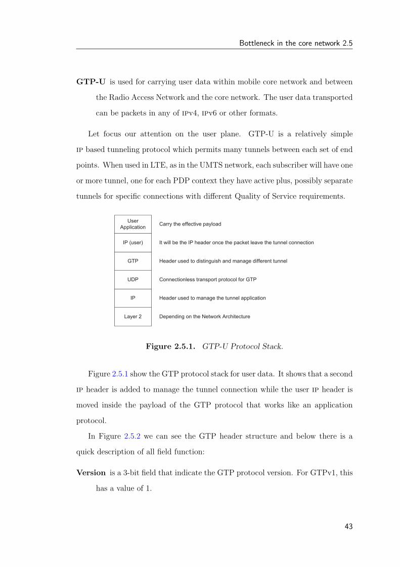
Bottleneck in the core network 2.5

GTP-U is used for carrying user data within mobile core network and between

the Radio Access Network and the core network. The user data transported

can be packets in any of ipv4, ipv6 or other formats.

Let focus our attention on the user plane. GTP-U is a relatively simple

ip based tunneling protocol which permits many tunnels between each set of end

points. When used in LTE, as in the UMTS network, each subscriber will have one

or more tunnel, one for each PDP context they have active plus, possibly separate

tunnels for specific connections with different Quality of Service requirements.

Layer 2

IP

UDP

GTP

UserApplication

IP (user)

Depending on the Network Architecture

Header used to manage the tunnel application

Connectionless transport protocol for GTP

Header used to distinguish and manage different tunnel

It will be the IP header once the packet leave the tunnel connection

Carry the effective payload

Figure 2.5.1. GTP-U Protocol Stack.

Figure 2.5.1 show the GTP protocol stack for user data. It shows that a second

ip header is added to manage the tunnel connection while the user ip header is

moved inside the payload of the GTP protocol that works like an application

protocol.

In Figure 2.5.2 we can see the GTP header structure and below there is a

quick description of all field function:

Version is a 3-bit field that indicate the GTP protocol version. For GTPv1, this

has a value of 1.

43

2. TCP and LTE

VersionProtpcol

TypeReserved

Next

Extension

Header

Sequence

Number

N-PDU

NumberType Total Lentht

Bits 0-2 3 4 5 6 7 8-15 16-23 24-31

0

32

64

TEID

Sequence NumberNext Extension

HeaderN-PDU Number

Figure 2.5.2. GTPv1 header (default and optional fields).

Protocol Type differentiates GTP (value 1) from GTP’ (value 0).

Reserved this field must be 0.

Extension Header (E) is set if there is an Extension Header optional field.

Sequence Number (S) is set if there is a Sequence Number optional field.

N-PDU number (PN) is set if there is a N-PDU number optional field.

Type differentiates the packet type

Total Length is a 16-bit field that states the length of the packet being encap-

sulated by GTP (not including the GTP header itself, but including the

optional fields).

Tunnel Endpoint Identifier (TEID) used to multiplex different connections

in the same GTP tunnel.

We can find also some optional fields available only if any of the E, S, or PN bits

are on. These fields are:

Sequence Number must be interpreted only if the S bit is set to 1.

N-PDU number must be interpreted only if the PN bit is high

44

Summary 2.6

Next Extension Header must be interpreted only if the E bit is on

The separate tunnels are identified by a Tunnel Endpoint Identifier (TEID) in

the GTP-U messages, which should be a dynamically allocated random number.

If this random number is of cryptographic quality, then it will provide a measure of

security against certain attacks. Even so, the requirement of the 3GPP standard

is that all GTP traffic, including user data should be sent within secure private

networks, not directly connected to the Internet.

2.6 Summary

In this chapter, an accurate description of the tcp protocol is given by focusing

on the flow control and congestion control. Particular attention is given to the

GTP tunnel protocol used by LTE during the handover procedure, where the

ip tunnel between the GW and the radio base station associated with the moving

mobile is switched in the GW towards the target base station when the terminal

arrives there. In the next chapter, we see how to manage TCP during LTE

handover.

45

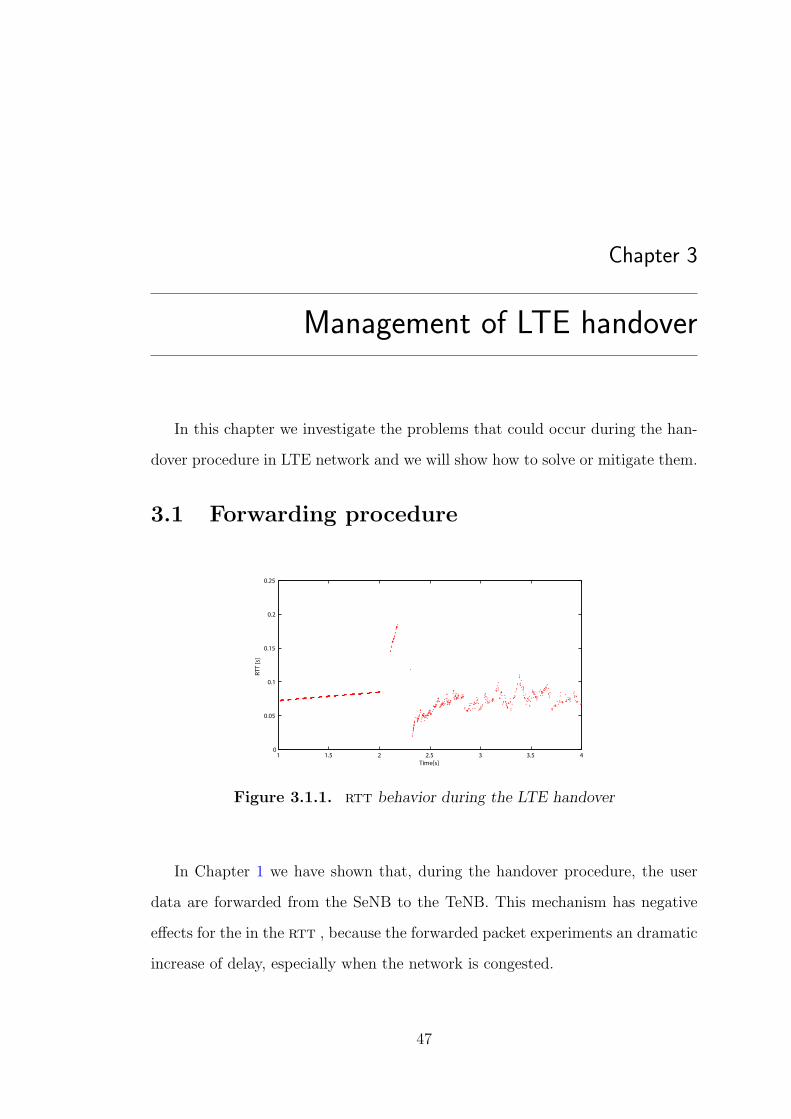
Chapter 3

Management of LTE handover

In this chapter we investigate the problems that could occur during the han-

dover procedure in LTE network and we will show how to solve or mitigate them.

3.1 Forwarding procedure

1 1.5 2 2.5 3 3.5 40

0.05

0.1

0.15

0.2

0.25

Time[s]

RTT

[s]

Figure 3.1.1. rtt behavior during the LTE handover

In Chapter 1 we have shown that, during the handover procedure, the user

data are forwarded from the SeNB to the TeNB. This mechanism has negative

effects for the in the rtt , because the forwarded packet experiments an dramatic

increase of delay, especially when the network is congested.

47

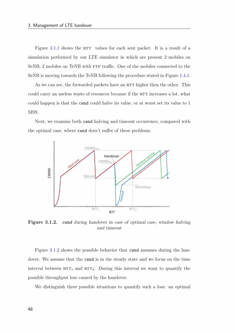
3. Management of LTE handover

Figure 3.1.1 shows the rtt values for each sent packet. It is a result of a

simulation performed by our LTE simulator in which are present 2 mobiles on

SeNB, 2 mobiles on TeNB with ftp traffic. One of the mobiles connected to the

SeNB is moving towards the TeNB following the procedure stated in Figure 1.4.1.

As we can see, the forwarded packets have an rtt higher then the other. This

could carry an useless waste of resources because if the rtt increases a lot, what

could happen is that the cwnd could halve its value, or at worst set its value to 1

MSS.

Next, we examine both cwnd halving and timeout occurrence, compared with

the optimal case, where cwnd does’t suffer of these problems.

Handover

SStresh

SStreshHO

CWNDMAX

CWNDHO

RTT1 RTT2RTT

CWN

D Ideal case

Window halving

Tim

eout

Figure 3.1.2. cwnd during handover in case of optimal case, window halvingand timeout

Figure 3.1.2 shows the possible behavior that cwnd assumes during the han-

dover. We assume that the cwnd is in the steady state and we focus on the time

interval between rtt1 and rtt2. During this interval we want to quantify the

possible throughput loss caused by the handover.

We distinguish three possible situations to quantify such a loss: an optimal

48

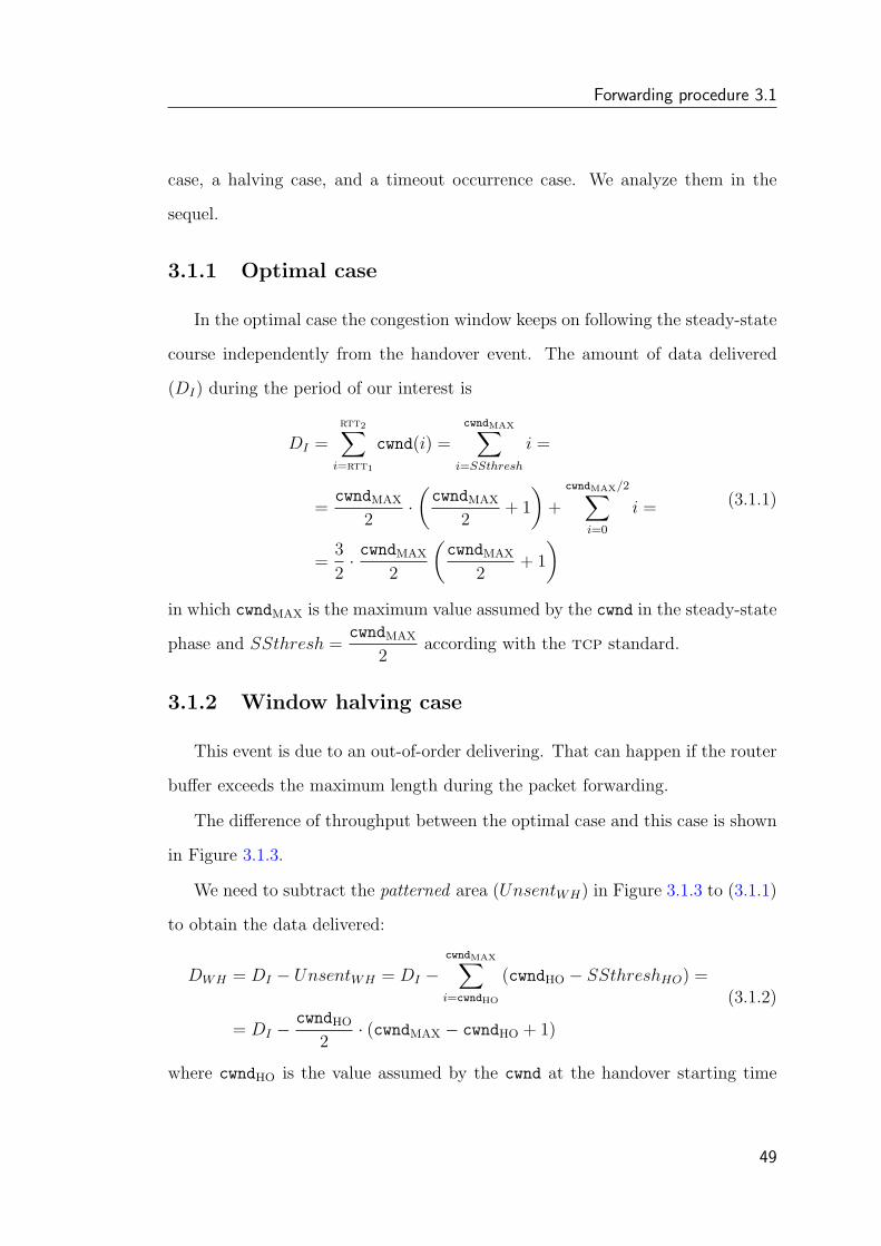
Forwarding procedure 3.1

case, a halving case, and a timeout occurrence case. We analyze them in the

sequel.

3.1.1 Optimal case

In the optimal case the congestion window keeps on following the steady-state

course independently from the handover event. The amount of data delivered

(DI) during the period of our interest is

DI =

rtt2∑i=rtt1

cwnd(i) =

cwndMAX∑i=SSthresh

i =

=cwndMAX

2·(cwndMAX

2+ 1

)+

cwndMAX/2∑i=0

i =

=3

2· cwndMAX

2

(cwndMAX

2+ 1

)(3.1.1)

in which cwndMAX is the maximum value assumed by the cwnd in the steady-state

phase and SSthresh =cwndMAX

2according with the tcp standard.

3.1.2 Window halving case

This event is due to an out-of-order delivering. That can happen if the router

buffer exceeds the maximum length during the packet forwarding.

The difference of throughput between the optimal case and this case is shown

in Figure 3.1.3.

We need to subtract the patterned area (UnsentWH) in Figure 3.1.3 to (3.1.1)

to obtain the data delivered:

DWH = DI − UnsentWH = DI −cwndMAX∑i=cwndHO

(cwndHO − SSthreshHO) =

= DI −cwndHO

2· (cwndMAX − cwndHO + 1)

(3.1.2)

where cwndHO is the value assumed by the cwnd at the handover starting time

49

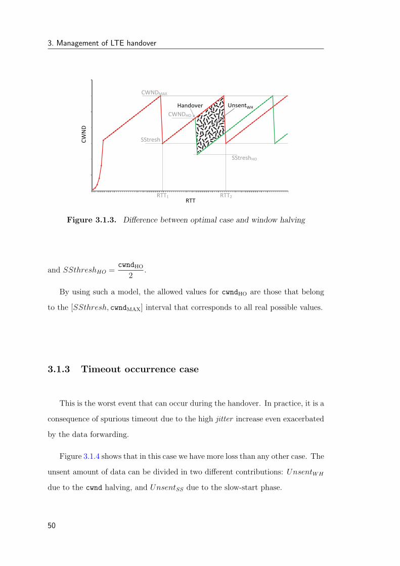
3. Management of LTE handover

Handover

SStresh

SStreshHO

CWNDMAX

CWNDHO

RTT1 RTT2RTT

CWN

D

UnsentWH

Figure 3.1.3. Difference between optimal case and window halving

and SSthreshHO =cwndHO

2.

By using such a model, the allowed values for cwndHO are those that belong

to the [SSthresh, cwndMAX] interval that corresponds to all real possible values.

3.1.3 Timeout occurrence case

This is the worst event that can occur during the handover. In practice, it is a

consequence of spurious timeout due to the high jitter increase even exacerbated

by the data forwarding.

Figure 3.1.4 shows that in this case we have more loss than any other case. The

unsent amount of data can be divided in two different contributions: UnsentWH

due to the cwnd halving, and UnsentSS due to the slow-start phase.

50

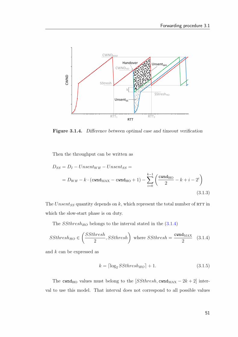
Forwarding procedure 3.1

Handover

SStresh

SStreshHO

CWNDMAX

CWNDHO

RTT1 RTT2RTT

CWN

D

k

UnsentWH

UnsentSS

Figure 3.1.4. Difference between optimal case and timeout verification

Then the throughput can be written as

DSS = DI − UnsentWH − UnsentSS =

= DWH − k · (cwndMAX − cwndHO + 1)−k−1∑i=0

(cwndHO

2− k + i− 2i

)(3.1.3)

The UnsentSS quantity depends on k, which represent the total number of rtt in

which the slow-start phase is on duty.

The SSthreshHO belongs to the interval stated in the (3.1.4)

SSthreshHO ∈(

SSthresh

2, SSthresh

)where SSthresh =

cwndMAX

2(3.1.4)

and k can be expressed as

k = dlog2 SSthreshHOe+ 1. (3.1.5)

The cwndHO values must belong to the [SSthresh, cwndMAX − 2k + 2] inter-

val to use this model. That interval does not correspond to all possible values

51

3. Management of LTE handover

40 45 50 55 60 65 70 75 8050

55

60

65

70

75

80

85

90

95

100

IdealWHSS

CWNDHO [Packets]

Nor

mal

ized

Thr

ough

put [

%]

(a) cwndMAX = 80.

70 80 90 100 110 12050

55

60

65

70

75

80

85

90

95

100

IdealWHSS

CWNDHO [Packets]

Nor

mal

ized

Thr

ough

put [

%]

(b) cwndMAX = 128.

140 160 180 200 220 24050

55

60

65

70

75

80

85

90

95

100

IdealWHSS

CWNDHO [Packets]

Nor

mal

ized

Thr

ough

put [

%]

(c) cwndMAX = 256.

Figure 3.1.5. Normalized throughput during the time interval (rtt1,rtt2)considering optimal case, window halving and timeout for different values of

cwndMAX

52

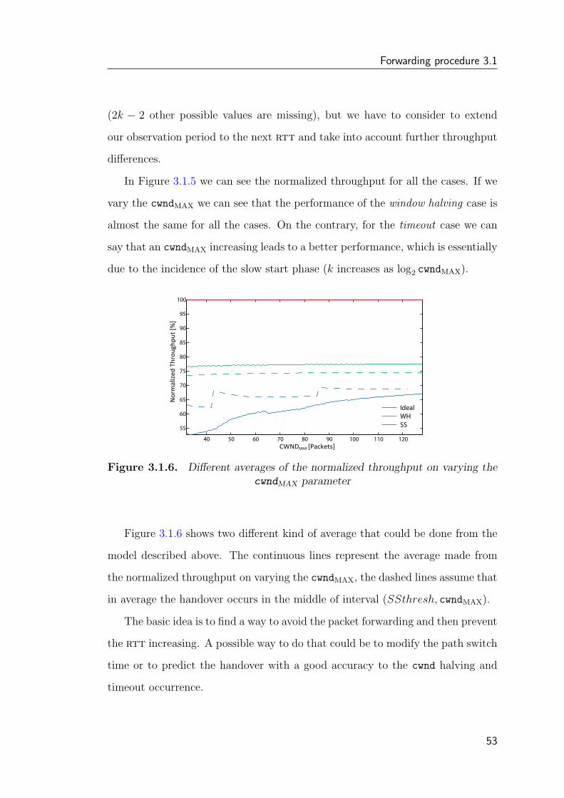
Forwarding procedure 3.1

(2k − 2 other possible values are missing), but we have to consider to extend

our observation period to the next rtt and take into account further throughput

differences.

In Figure 3.1.5 we can see the normalized throughput for all the cases. If we

vary the cwndMAX we can see that the performance of the window halving case is

almost the same for all the cases. On the contrary, for the timeout case we can

say that an cwndMAX increasing leads to a better performance, which is essentially

due to the incidence of the slow start phase (k increases as log2 cwndMAX).

40 50 60 70 80 90 100 110 120

55

60

65

70

75

80

85

90

95

100

CWNDMAX [Packets]

Nor

mal

ized

Thr

ough

put [

%]

IdealWHSS

Figure 3.1.6. Different averages of the normalized throughput on varying thecwndMAX parameter

Figure 3.1.6 shows two different kind of average that could be done from the

model described above. The continuous lines represent the average made from

the normalized throughput on varying the cwndMAX, the dashed lines assume that

in average the handover occurs in the middle of interval (SSthresh, cwndMAX).

The basic idea is to find a way to avoid the packet forwarding and then prevent

the rtt increasing. A possible way to do that could be to modify the path switch

time or to predict the handover with a good accuracy to the cwnd halving and

timeout occurrence.

53

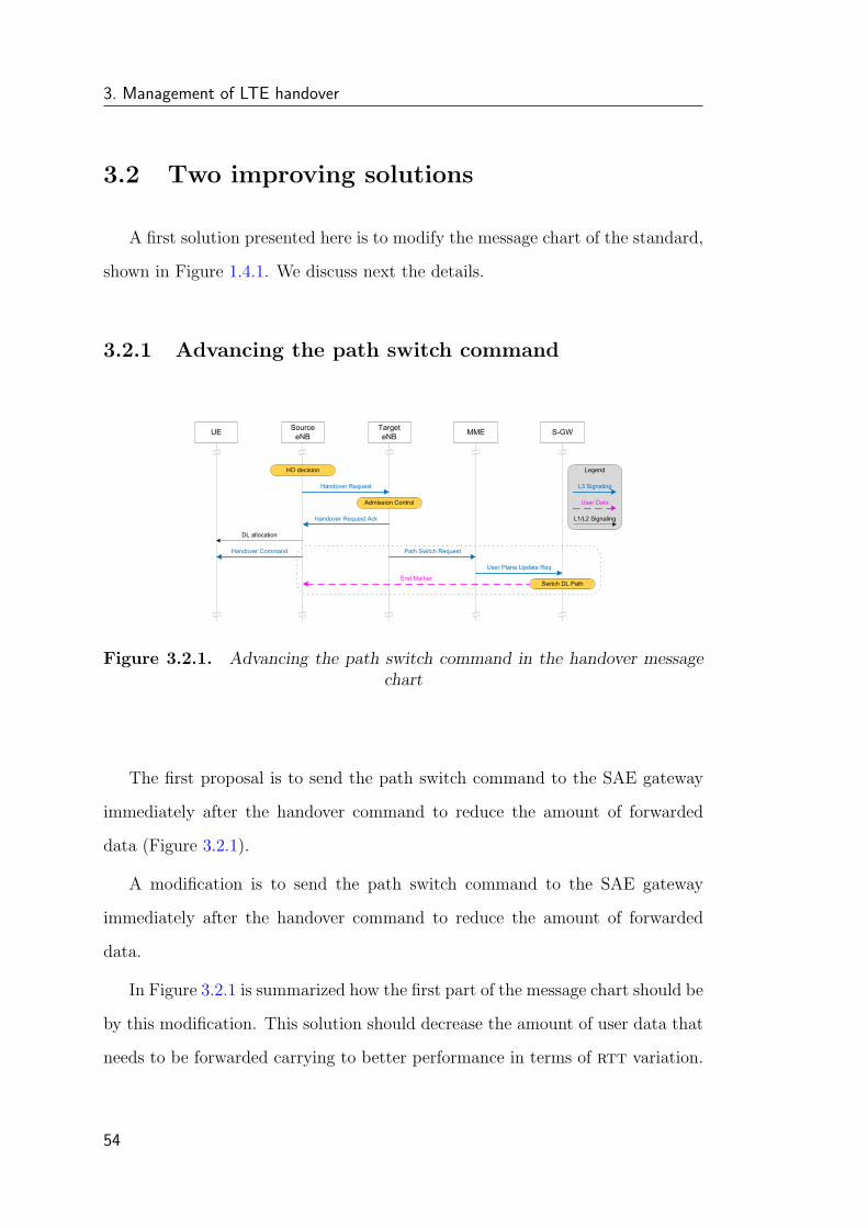
3. Management of LTE handover

3.2 Two improving solutions

A first solution presented here is to modify the message chart of the standard,

shown in Figure 1.4.1. We discuss next the details.

3.2.1 Advancing the path switch command

UE SourceeNB

TargeteNB MME S-GW

HO decision

Handover Request

Handover Request Ack

Admission Control

DL allocation

Handover Command Path Switch Request

User Plane Update Req

Switch DL PathEnd Marker

L3 Signaling

User Data

L1/L2 Signaling

Legend

Figure 3.2.1. Advancing the path switch command in the handover messagechart

The first proposal is to send the path switch command to the SAE gateway

immediately after the handover command to reduce the amount of forwarded

data (Figure 3.2.1).

A modification is to send the path switch command to the SAE gateway

immediately after the handover command to reduce the amount of forwarded

data.

In Figure 3.2.1 is summarized how the first part of the message chart should be

by this modification. This solution should decrease the amount of user data that

needs to be forwarded carrying to better performance in terms of rtt variation.

54

Two improving solutions 3.2

3.2.2 Predicting the handover occurrence

The second proposal is using a handover prediction mechanism. Even if in the

LTE standard this feature is not used yet, it seems to be an appealing solution

for a 3G LTE system.

The basic idea of this solution concerns a prediction of the handover event to

allow the generation of the path switch command before the handover command.

This algorithm allow the emptying of the ME pipe before the handover command

and avoid the data forwarding procedure, as shown in Figure 3.2.2.

UESource

eNB

Target

eNBMME S-GW

HO prediction

Handover Request

Handover Request Ack

Admission Control

DL allocation

Handover Command

Path Switch Request

User Plane Update Req

Switch DL PathEnd Marker

L3 Signaling

User Data

L1/L2 Signaling

Legend

1. Measurement Control

Packet Data

UL allocation

2. Measurement Report

Ne

ce

ssa

ry P

red

ictio

n tim

e in

terv

al

Figure 3.2.2. Modification to the handover message chart to predict the han-dover.

In this case the modification in the message chart involves that the path switch

request should be sent to the MME before the handover (Figure 3.2.2). In that

way the amount of user data that need to be forwarded should decrease, carrying

to better performance in terms of rtt variation.

For this solution, as well as for the one depicted in the Section 3.2.1, a pro-

cedure is needed for resource allocation on the Target eNB after a request made

55

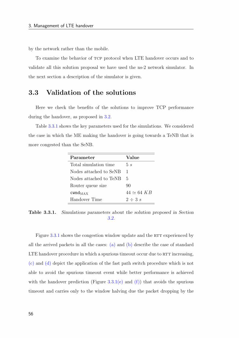
3. Management of LTE handover

by the network rather than the mobile.

To examine the behavior of tcp protocol when LTE handover occurs and to

validate all this solution proposal we have used the ns-2 network simulator. In

the next section a description of the simulator is given.

3.3 Validation of the solutions

Here we check the benefits of the solutions to improve TCP performance

during the handover, as proposed in 3.2.

Table 3.3.1 shows the key parameters used for the simulations. We considered

the case in which the ME making the handover is going towards a TeNB that is

more congested than the SeNB.

Parameter Value

Total simulation time 5 s

Nodes attached to SeNB 1

Nodes attached to TeNB 5

Router queue size 90

cwndMAX 44 ' 64 KB

Handover Time 2 ÷ 3 s

Table 3.3.1. Simulations parameters about the solution proposed in Section3.2.

Figure 3.3.1 shows the congestion window update and the rtt experienced by

all the arrived packets in all the cases: (a) and (b) describe the case of standard

LTE handover procedure in which a spurious timeout occur due to rtt increasing,

(c) and (d) depict the application of the fast path switch procedure which is not

able to avoid the spurious timeout event while better performance is achieved

with the handover prediction (Figure 3.3.1(e) and (f)) that avoids the spurious

timeout and carries only to the window halving due the packet dropping by the

56

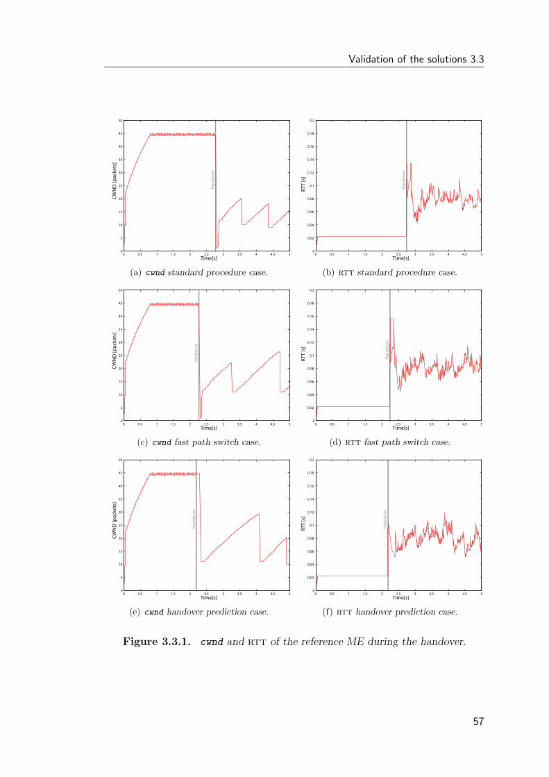
Validation of the solutions 3.3

0 0.5 1 1.5 2 2.5 3 3.5 4 4.5 50

5

10

15

20

25

30

35

40

45

50

Time[s]

CWN

D [p

acke

ts]

Han

dove

r

(a) cwnd standard procedure case.

0 0.5 1 1.5 2 2.5 3 3.5 4 4.5 50

0.02

0.04

0.06

0.08

0.1

0.12

0.14

0.16

0.18

0.2

Time[s]

RTT

[s]

Han

dove

r

(b) rtt standard procedure case.

0 0.5 1 1.5 2 2.5 3 3.5 4 4.5 50

5

10

15

20

25

30

35

40

45

50

Time[s]

CWN

D [p

acke

ts]

Han

dove

r

(c) cwnd fast path switch case.

0 0.5 1 1.5 2 2.5 3 3.5 4 4.5 50

0.02

0.04

0.06

0.08

0.1

0.12

0.14

0.16

0.18

0.2

Time[s]

RTT

[s]

Han

dove

r

(d) rtt fast path switch case.

0 0.5 1 1.5 2 2.5 3 3.5 4 4.5 50

5

10

15

20

25

30

35

40

45

50

Time[s]

CWN

D [p

acke

ts]

Han

dove

r

(e) cwnd handover prediction case.

0 0.5 1 1.5 2 2.5 3 3.5 4 4.5 50

0.02

0.04

0.06

0.08

0.1

0.12

0.14

0.16

0.18

0.2

Time[s]

RTT

[s]

Han

dove

r

(f) rtt handover prediction case.

Figure 3.3.1. cwnd and rtt of the reference ME during the handover.

57

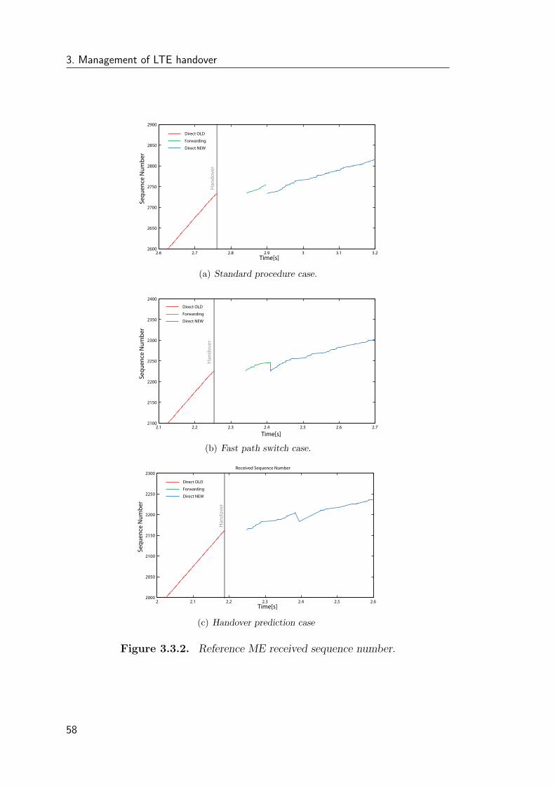
3. Management of LTE handover

2.6 2.7 2.8 2.9 3 3.1 3.22600

2650

2700

2750

2800

2850

2900

Time[s]

Sequ

ence

Num

ber

Direct OLD

Forwarding

Direct NEW

Han

dove

r

(a) Standard procedure case.

2.1 2.2 2.3 2.4 2.5 2.6 2.72100

2150

2200

2250

2300

2350

2400

Time[s]

Sequ

ence

Num

ber

Direct OLD

Forwarding

Direct NEW

Han

dove

r

(b) Fast path switch case.

2 2.1 2.2 2.3 2.4 2.5 2.62000

2050

2100

2150

2200

2250

2300Received Sequence Number

Time[s]

Sequ

ence

Num

ber

Direct OLD

Forwarding

Direct NEW

Han

dove

r

(c) Handover prediction case

Figure 3.3.2. Reference ME received sequence number.

58

Summary 3.4

router buffer.

In Figure 3.3.2 we can see that between standard handover procedure and

fast path switch procedure there is a negligible difference in terms of amount of

data forwarded (green line in the Figure 3.3.2(a) and (b)), this is essentially due

to the fact that outstanding data always corresponds to the window, intended as

in (2.2.1), and at the handover time such an amount of data has been already

pushed in the network. On the contrary, there are no forwarded data in the

handover prediction procedure (Figure 3.3.2(c)) and that is the main reason that

carrying to better performance.

3.4 Summary

In this chapter the main issues of the LTE handover procedure are investi-

gated. After a study regarding the possible tcp behavior, two solutions proposed

and validated by simulation in ns-2. These solutions avoids the data forwarding

during the LTE handover, and thus they improve the performance of the tcp pro-

tocol as seen by the end-user.

59

Chapter 4

LTE simulator: an overview

In this chapter a brief description of the ns-2 LTE simulator and the nsMir-

acle framework is given to show how we implemented our LTE simulator. This

simulator is the first one developed to evaluate LTE performance in ns2. We use

it to validate the solution proposed in Chapter 3 and the model proposed in the

next chapter.

4.1 LTE simulator through ns-2 and nsMiracle

ns began as a variant of the REAL network simulator in 1989 and has evolved

substantially over the past few years. In 1995 ns development was supported

by DARPA through the VINT project [27] at LBL, Xerox PARC, UCB, and

USC/ISI. Currently ns development is support through DARPA with SAMAN

and through NSF with CONSER, both in collaboration with other researchers

including ACIRI. ns has always included substantial contributions from other

researchers, including wireless code from the UCB Daedelus and CMU Monarch

projects and Sun Microsystems. We used the version 2 of ns, called ns-2.

ns-2 is a discrete event simulator targeted at networking research that provides

substantial support for simulation of tcp, routing, and multicast protocols over

wired and wireless (local and satellite) networks. ns-2 is written in C++ and an

61

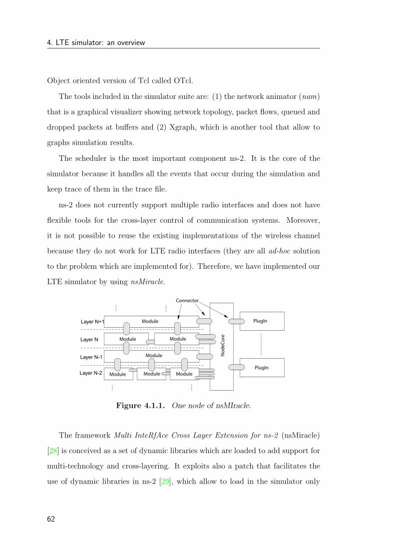
4. LTE simulator: an overview

Object oriented version of Tcl called OTcl.

The tools included in the simulator suite are: (1) the network animator (nam)

that is a graphical visualizer showing network topology, packet flows, queued and

dropped packets at buffers and (2) Xgraph, which is another tool that allow to

graphs simulation results.

The scheduler is the most important component ns-2. It is the core of the

simulator because it handles all the events that occur during the simulation and

keep trace of them in the trace file.

ns-2 does not currently support multiple radio interfaces and does not have

flexible tools for the cross-layer control of communication systems. Moreover,

it is not possible to reuse the existing implementations of the wireless channel

because they do not work for LTE radio interfaces (they are all ad-hoc solution

to the problem which are implemented for). Therefore, we have implemented our

LTE simulator by using nsMiracle.

.....

.....

.....

......

......

.....

.....

Layer N+1

Layer N

Layer N-1

Layer N-2

Module

Module

Module

Module

Connector

PlugIn

PlugInModuleModuleModule

Nod

eCore

Figure 4.1.1. One node of nsMIracle.

The framework Multi InteRfAce Cross Layer Extension for ns-2 (nsMiracle)

[28] is conceived as a set of dynamic libraries which are loaded to add support for

multi-technology and cross-layering. It exploits also a patch that facilitates the

use of dynamic libraries in ns-2 [29], which allow to load in the simulator only

62

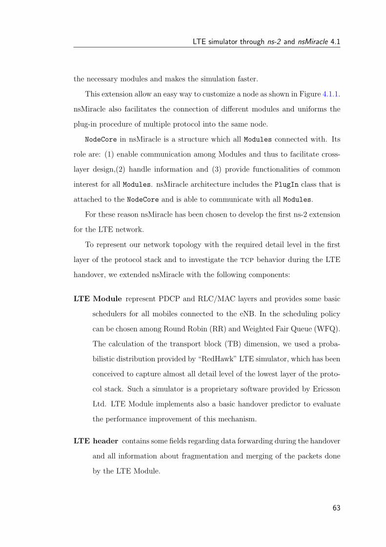
LTE simulator through ns-2 and nsMiracle 4.1

the necessary modules and makes the simulation faster.

This extension allow an easy way to customize a node as shown in Figure 4.1.1.

nsMiracle also facilitates the connection of different modules and uniforms the

plug-in procedure of multiple protocol into the same node.

NodeCore in nsMiracle is a structure which all Modules connected with. Its

role are: (1) enable communication among Modules and thus to facilitate cross-

layer design,(2) handle information and (3) provide functionalities of common

interest for all Modules. nsMiracle architecture includes the PlugIn class that is

attached to the NodeCore and is able to communicate with all Modules.

For these reason nsMiracle has been chosen to develop the first ns-2 extension

for the LTE network.

To represent our network topology with the required detail level in the first

layer of the protocol stack and to investigate the tcp behavior during the LTE

handover, we extended nsMiracle with the following components:

LTE Module represent PDCP and RLC/MAC layers and provides some basic

schedulers for all mobiles connected to the eNB. In the scheduling policy

can be chosen among Round Robin (RR) and Weighted Fair Queue (WFQ).

The calculation of the transport block (TB) dimension, we used a proba-

bilistic distribution provided by “RedHawk” LTE simulator, which has been

conceived to capture almost all detail level of the lowest layer of the proto-

col stack. Such a simulator is a proprietary software provided by Ericsson

Ltd. LTE Module implements also a basic handover predictor to evaluate

the performance improvement of this mechanism.

LTE header contains some fields regarding data forwarding during the handover

and all information about fragmentation and merging of the packets done

by the LTE Module.

63

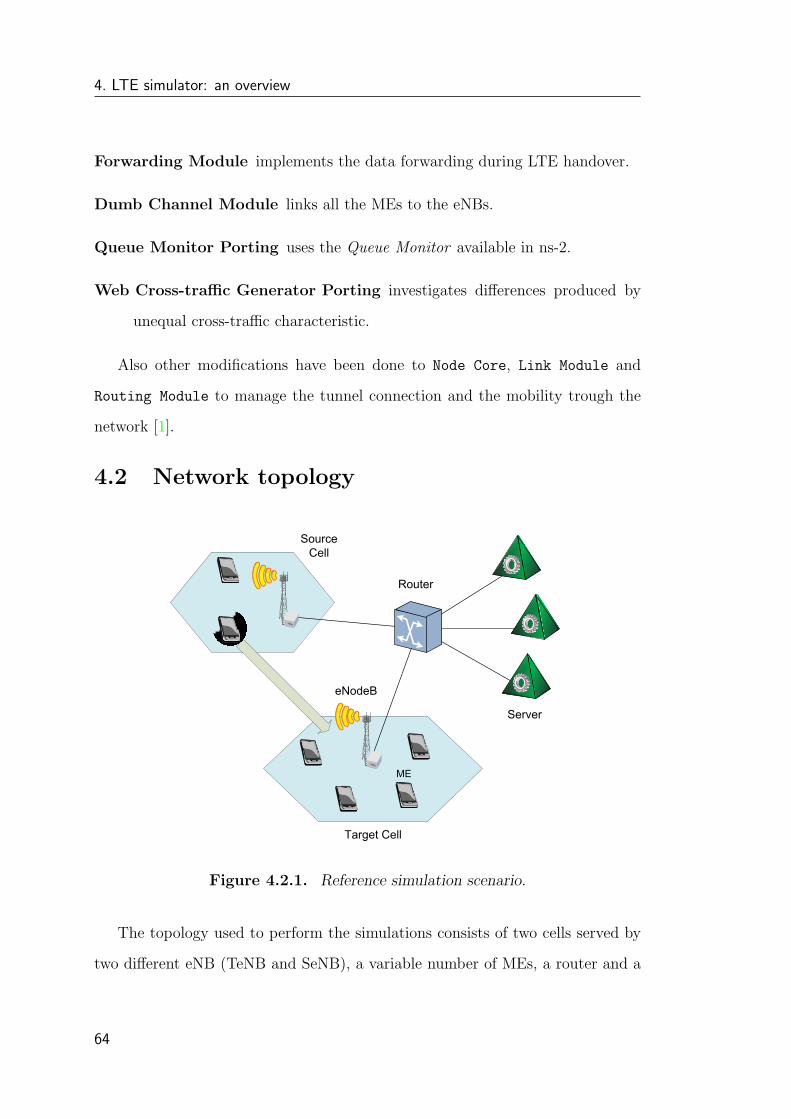
4. LTE simulator: an overview

Forwarding Module implements the data forwarding during LTE handover.

Dumb Channel Module links all the MEs to the eNBs.

Queue Monitor Porting uses the Queue Monitor available in ns-2.

Web Cross-traffic Generator Porting investigates differences produced by

unequal cross-traffic characteristic.

Also other modifications have been done to Node Core, Link Module and

Routing Module to manage the tunnel connection and the mobility trough the

network [1].

4.2 Network topology

SourceCell

eNodeB

Router

Server

ME

Target Cell

Figure 4.2.1. Reference simulation scenario.

The topology used to perform the simulations consists of two cells served by

two different eNB (TeNB and SeNB), a variable number of MEs, a router and a

64

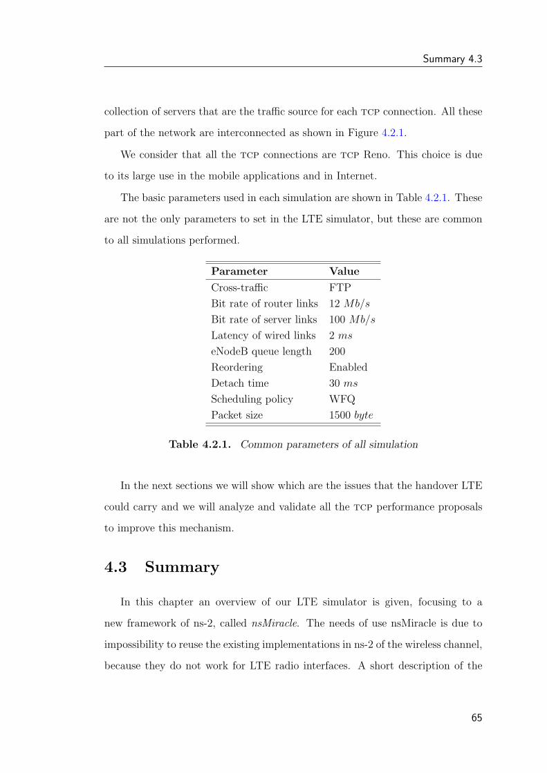
Summary 4.3

collection of servers that are the traffic source for each tcp connection. All these

part of the network are interconnected as shown in Figure 4.2.1.

We consider that all the tcp connections are tcp Reno. This choice is due

to its large use in the mobile applications and in Internet.

The basic parameters used in each simulation are shown in Table 4.2.1. These

are not the only parameters to set in the LTE simulator, but these are common

to all simulations performed.

Parameter Value

Cross-traffic FTP

Bit rate of router links 12 Mb/s

Bit rate of server links 100 Mb/s

Latency of wired links 2 ms

eNodeB queue length 200

Reordering Enabled

Detach time 30 ms

Scheduling policy WFQ

Packet size 1500 byte

Table 4.2.1. Common parameters of all simulation

In the next sections we will show which are the issues that the handover LTE

could carry and we will analyze and validate all the tcp performance proposals

to improve this mechanism.

4.3 Summary

In this chapter an overview of our LTE simulator is given, focusing to a

new framework of ns-2, called nsMiracle. The needs of use nsMiracle is due to

impossibility to reuse the existing implementations in ns-2 of the wireless channel,

because they do not work for LTE radio interfaces. A short description of the

65

4. LTE simulator: an overview

nsMiracle node is also given and the network topology implemented is shown with

some implementation parameters set to achieve the aims of this project.

66

Chapter 5

Mathematical model of TCP over LTE

In this Chapter we propose a mathematical model of the tcp during the

handover in LTE. The model is then validated by ns-2 simulations.

To develop a model that is able to capture the important dynamics of the real

system and, at the same time, be simple enough for mathematical analysis, we

have to know which class of models we want to use. There are three classes of

mathematical models fo congestion control: packet-level, fluid flow and hybrid.

The first one sees the network from a discrete-events point of view; so, it takes

into account the location of each individual packet. The second one describes

the network system using differential equation; this mean that this model does

not take into account the packet boundaries, but sees the data transport as a

continuous flow. All the quantities of interest, such as sending rates, window

sizes and queue sizes, are considered as continuous functions of time. The last

one is a result of discrete events, together with continuous changes between events.

Next a deep description of the analytical model is given taking into account the

LTE an tcp concept explained in the first chapters.

67

5. Mathematical model of TCP over LTE

5.1 Existing models

In the literature, the following models to describe the behavior of congestion

control can be found:

1. Integrator model

2. Static link model

3. Joint link model

4. DAE link model

Before analyzing the models listed above, we make some useful considerations.

First, when analyzing congestion control methods, it is useful to divide the sys-

tem traffic into two types: Traffic from flows that use congestion control, and

other cross traffic, x(t) (cross traffic). Second, in fluid flow modeling of queueing

networks, data rates are the central quantities of interest. In the tcp family

of congestion control, the main control variable is the congestion window. The

sending rate is determined indirectly by the window size, under the control of the

ack-clock. For equilibrium or average quantities, that relation between window

size and the resulting sending rate is simple:

sending rate =window size

roundtrip time. (5.1.1)

At this point is better to understand what the “windows size” is. We mean by

“windows size” (w(t)) the actual amount of in-flight data, which are packets that

have been transmitted but for which no ack has been received yet. Sometimes

this definition may create a confusion with congestion window in tcp, cwnd, which

is determined by the window update mechanism, but there may be a significant

discrepancy between w and cwnd.

68

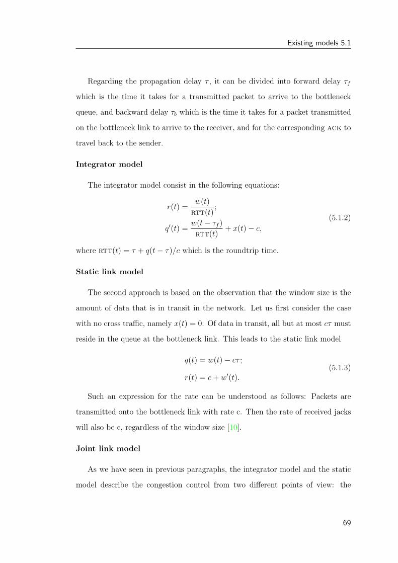
Existing models 5.1

Regarding the propagation delay τ , it can be divided into forward delay τf

which is the time it takes for a transmitted packet to arrive to the bottleneck

queue, and backward delay τb which is the time it takes for a packet transmitted

on the bottleneck link to arrive to the receiver, and for the corresponding ack to

travel back to the sender.

Integrator model

The integrator model consist in the following equations:

r(t) =w(t)

rtt(t);

q′(t) =w(t− τf )

rtt(t)+ x(t)− c,

(5.1.2)

where rtt(t) = τ + q(t− τ)/c which is the roundtrip time.

Static link model

The second approach is based on the observation that the window size is the

amount of data that is in transit in the network. Let us first consider the case

with no cross traffic, namely x(t) = 0. Of data in transit, all but at most cτ must

reside in the queue at the bottleneck link. This leads to the static link model

q(t) = w(t)− cτ ;

r(t) = c + w′(t).(5.1.3)

Such an expression for the rate can be understood as follows: Packets are

transmitted onto the bottleneck link with rate c. Then the rate of received jacks

will also be c, regardless of the window size [10].

Joint link model

As we have seen in previous paragraphs, the integrator model and the static

model describe the congestion control from two different points of view: the

69

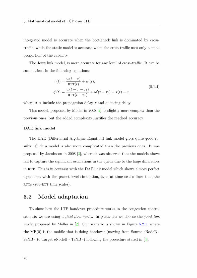
5. Mathematical model of TCP over LTE

integrator model is accurate when the bottleneck link is dominated by cross-

traffic, while the static model is accurate when the cross-traffic uses only a small

proportion of the capacity.

The Joint link model, is more accurate for any level of cross-traffic. It can be

summarized in the following equations:

r(t) =w(t− τ)

rtt(t)+ w′(t);

q′(t) =w(t− τ − τf )

rtt(t− τf )+ w′(t− τf ) + x(t)− c,

(5.1.4)

where rtt include the propagation delay τ and queueing delay.

This model, proposed by Moller in 2008 [2], is slightly more complex than the

previous ones, but the added complexity justifies the reached accuracy.

DAE link model

The DAE (Differential Algebraic Equation) link model gives quite good re-

sults. Such a model is also more complicated than the previous ones. It was

proposed by Jacobsson in 2008 [3], where it was observed that the models above

fail to capture the significant oscillations in the queue due to the large differences

in rtt. This is in contrast with the DAE link model which shows almost perfect

agreement with the packet level simulation, even at time scales finer than the

rtts (sub-rtt time scales).

5.2 Model adaptation

To show how the LTE handover procedure works in the congestion control

scenario we are using a fluid-flow model. In particular we choose the joint link

model proposed by Moller in [2]. Our scenario is shown in Figure 5.2.1, where

the ME(0) is the mobile that is doing handover (moving from Source eNodeB -

SeNB - to Target eNodeB - TeNB -) following the procedure stated in [4].

70

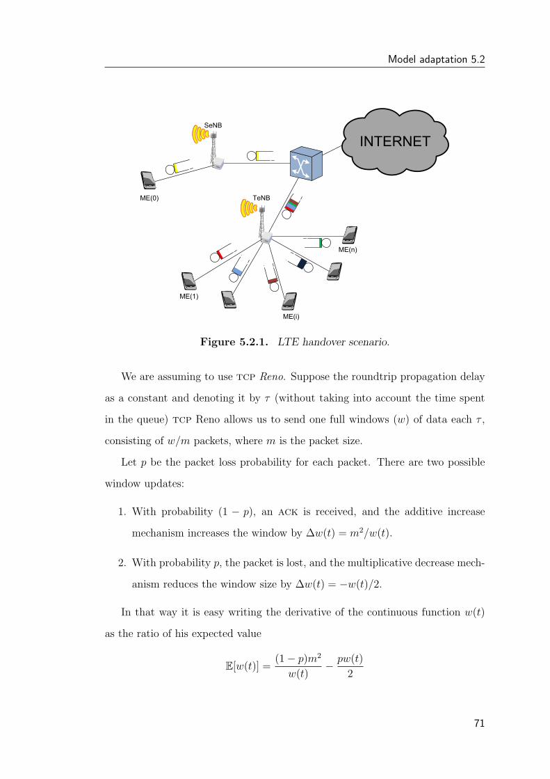
Model adaptation 5.2

SeNB

TeNBME(0)

ME(1)

ME(n)

ME(i)

INTERNET

Figure 5.2.1. LTE handover scenario.

We are assuming to use tcp Reno. Suppose the roundtrip propagation delay

as a constant and denoting it by τ (without taking into account the time spent

in the queue) tcp Reno allows us to send one full windows (w) of data each τ ,

consisting of w/m packets, where m is the packet size.

Let p be the packet loss probability for each packet. There are two possible

window updates:

1. With probability (1 − p), an ack is received, and the additive increase

mechanism increases the window by ∆w(t) = m2/w(t).

2. With probability p, the packet is lost, and the multiplicative decrease mech-

anism reduces the window size by ∆w(t) = −w(t)/2.

In that way it is easy writing the derivative of the continuous function w(t)

as the ratio of his expected value

E[w(t)] =(1− p)m2

w(t)− pw(t)

2

71

5. Mathematical model of TCP over LTE

and the average inter-packet time T = τm/w:

dw

dt=

(1− p)m

τ− pw2(t)

2τm. (5.2.1)

By extending this result with the time-varying queueing delay, (5.2.1) becomes

dw

dt=

(1− p)m

τ + q(t− τb)/c− pw2(t)

2m (τ + q(t− τb)/c), (5.2.2)

where c is the link capacity and τb is the backward delay.

5.2.1 Single flow and multiple flow model

In the previous section is shown that for single flow traversing a single bottle-

neck, the state equations are

r(t) =w(t− τ)

rtt(t)+ w′(t);

q′(t) =w(t− τ − τf )

rtt(t− τf )+ w′(t− τf ) + x(t)− c,

(5.2.3)

where w′(t) is defined by (5.2.2) for tcp Reno, x(t) is the cross traffic (it includes

all non tcp traffic type) and rtt(t) = τ + q(t− τb)/c, where τ = τf + τb. τf and

τb are the forward and backward delay, respectively.

When we have multiple flows traversing a single bottleneck, every k-th ones

have a window size wk(t), sending rate rk(t), and a roundtrip propagation delay

τk. Let us extend the results found in (5.2.3), below is shown how we can easily

write the equation for multiple flows. Without loss of generality, we can assume

that τf,k = 0.

rk(t) =wk(t− τk)

rttk(t)+ w′

k(t),

q′(t) =∑

k

wk(t− τk)

rttk(t)+

∑k

w′k(t) + x(t)− c,

(5.2.4)

where now rttk(t) = τ + q(t− τk)/c, in which τk = τb,k.

72

Application scenario 5.3

Flows with the same roundtrip propagation delay behave as a single aggre-

gated flow, where the rate and the window size of the aggregated packets are the

sums of the rate and window sizes of the individual flows. With heterogeneous

delays, the dynamics becomes more complex.

5.3 Application scenario

In this section we apply the model illustrated before to our scenario by dividing

the problem in three phases:

1. Handover preparation: the ME(0) is still attached to the network by the

SeNB and other mobiles are connected with TeNB;

2. Handover actuation: this phase is the time in which the mobile ME(0)

starts the handover procedure (at time tHO) and his data - stored in the

SeNB’s buffer - start to be forwarded to TeNB through the core network

(Router);

3. Handover completion: the handover has finished and the ME(0) is at-

tached to the network by the TeNB with all the other mobiles and share

the radio resource with them.

5.3.1 Handover preparation

In the beginning we suppose that the ME(0) is the only mobile attached to

SeNB, so we start the analysis by studying the queue state over the link between

the router and SeNB (see Figure 5.2.1) taking into account that all the connection

between MEs and sources are tcp ones, so we can handle this problem as a single

tcp flow traversing a single bottleneck. The state equation are given by (5.2.3).

Meanwhile, studying the queue state over the link between the router and

TeNB (see Figure 5.2.1), we can suppose to handle the problem as a multiple

73

5. Mathematical model of TCP over LTE

tcp flows traversing a single bottleneck; so the state equation will become (5.2.4)

with 1 ≤ k < n, where n is the total number of attached mobiles to the TeNB.

5.3.2 Handover actuation

At the handover time, tHO, we suppose that all the data in the SeNB’s buffer

are moved to the TeNB’s buffer in a priority queue to avoid the out of order

packets arrival to ME(0). Hence, the packet amount that are forwarded to the

TeNB at time tHO, is the in-flight data at tHO added to the data sent from the

sources, between the attach time (tATT ) and path sw time (tPS), which is 10ms

for LTE. We call by FW this packet amount. We model this data transfer as the

time that a link with capacity c uses to transmit FW data; in that way, the integral

is exactly the data to forwards. Specifically, for the ME(0) in the TeNB, we have

(denoting his flow by k = 0) that

r0(t) =w(t− τ0)

rtt0(t)+ w′

0(t);

q′0(t) =w(t− τ0)

rtt0(t)+ w′(t− τ0) + x(t)− c + c · rect

(t− (tHO + FW/2c)

FW/c

),

(5.3.1)

where

FW = w(tHO) +

∫ tPS

tATT

r0(t)dt (5.3.2)

and for all the other flows the equations are given by (5.2.4).

5.3.3 Handover completion

After handover at TeNB the situation will be the same as before, with the

exception of the presence of a further mobile. Therefore, the equations for all the

flows are given by (5.2.4) but now 0 ≤ k < n. At SeNB we don’t have anymore

tcp connections.

74

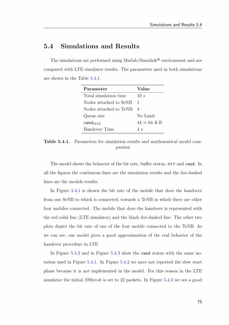
Simulations and Results 5.4

5.4 Simulations and Results

The simulations are performed using Matlab/Simulinkr environment and are

compared with LTE simulator results. The parameters used in both simulations

are shown in the Table 5.4.1.

Parameter Value

Total simulation time 10 s

Nodes attached to SeNB 1

Nodes attached to TeNB 4

Queue size No Limit

cwndMAX 44 ' 64 KB

Handover Time 4 s

Table 5.4.1. Parameters for simulation results and mathematical model com-parison

The model shows the behavior of the bit rate, buffer status, rtt and cwnd. In

all the figures the continuous lines are the simulation results and the dot-dashed

lines are the models results.

In Figure 5.4.1 is shown the bit rate of the mobile that does the handover

from one SeNB to which is connected, towards a TeNB in which there are other

four mobiles connected. The mobile that does the handover is represented with

the red solid line (LTE simulator) and the black dot-dashed line. The other two

plots depict the bit rate of one of the four mobile connected to the TeNB. As

we can see, our model gives a good approximation of the real behavior of the

handover procedure in LTE.

In Figure 5.4.2 and in Figure 5.4.3 show the cwnd status with the same no-

tation used in Figure 5.4.1. In Figure 5.4.2 we nave not reported the slow start

phase because it is not implemented in the model. For this reason in the LTE

simulator the initial SSthresh is set to 22 packets. In Figure 5.4.3 we see a good

75

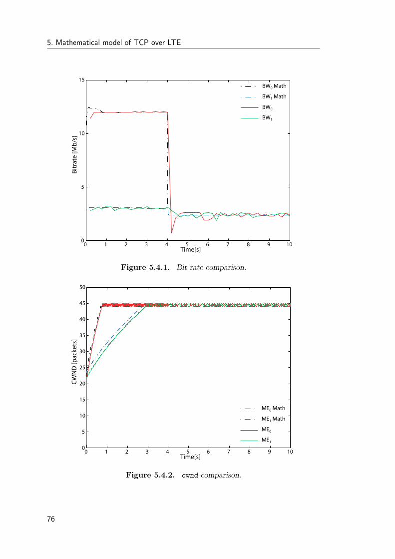
5. Mathematical model of TCP over LTE

0 1 2 3 4 5 6 7 8 9 100

5

10

15

Time[s]

Bitr

ate

[Mb/

s]

BW0 Math

BW1 Math

BW0

BW1

Figure 5.4.1. Bit rate comparison.

0 1 2 3 4 5 6 7 8 9 100

5

10

15

20

25

30

35

40

45

50

Time[s]

CWN

D [p

acke

ts]

ME0 Math

ME1 Math

ME0

ME1

Figure 5.4.2. cwnd comparison.

76

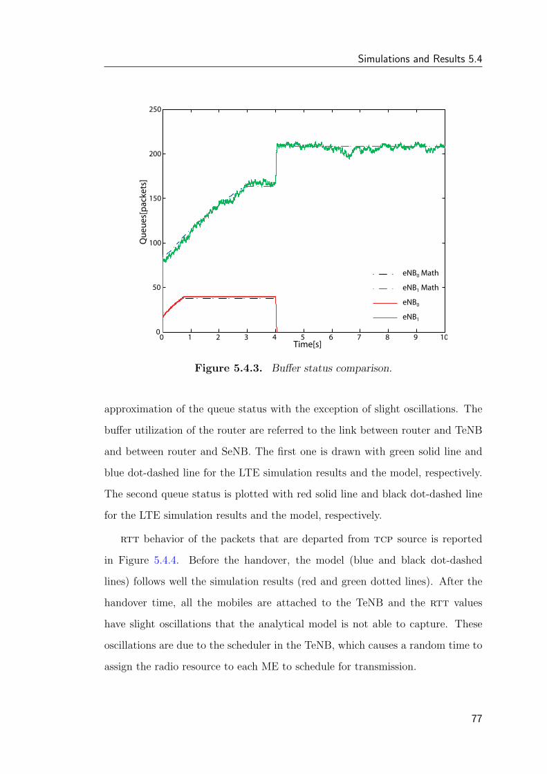
Simulations and Results 5.4

0 1 2 3 4 5 6 7 8 9 100

50

100

150

200

250

Time[s]

Que

ues[

pack

ets]

eNB0 Math

eNB1 Math

eNB0

eNB1

Figure 5.4.3. Buffer status comparison.

approximation of the queue status with the exception of slight oscillations. The

buffer utilization of the router are referred to the link between router and TeNB

and between router and SeNB. The first one is drawn with green solid line and

blue dot-dashed line for the LTE simulation results and the model, respectively.

The second queue status is plotted with red solid line and black dot-dashed line

for the LTE simulation results and the model, respectively.

rtt behavior of the packets that are departed from tcp source is reported

in Figure 5.4.4. Before the handover, the model (blue and black dot-dashed

lines) follows well the simulation results (red and green dotted lines). After the

handover time, all the mobiles are attached to the TeNB and the rtt values

have slight oscillations that the analytical model is not able to capture. These

oscillations are due to the scheduler in the TeNB, which causes a random time to

assign the radio resource to each ME to schedule for transmission.

77

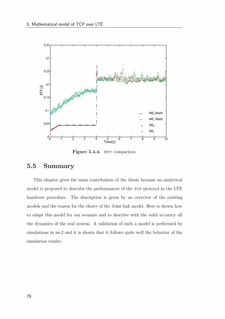
5. Mathematical model of TCP over LTE

0 1 2 3 4 5 6 7 8 9 100

0.05

0.1

0.15

0.2

0.25

0.3

0.35

Time[s]

RTT

[s]

ME0 Math

ME1 Math

ME0

ME1

Figure 5.4.4. rtt comparison.

5.5 Summary

This chapter gives the main contribution of the thesis because an analytical

model is proposed to describe the performances of the tcp protocol in the LTE

handover procedure. The description is given by an overview of the existing

models and the reason for the choice of the Joint link model. Here is shown how

to adapt this model for our scenario and to describe with the valid accuracy all

the dynamics of the real system. A validation of such a model is performed by

simulations in ns-2 and it is shown that it follows quite well the behavior of the

simulation results.

78

Chapter 6

Conclusion and future work

6.1 Conclusion

In this thesis we have studied the impacts on the end-user and system per-

formance when users with high bit rates tcp services are moving through the

network. In particular we have focused on the tcp performances during the LTE

handover procedure.

To reach such an aim we proposed a simple modification of the analytical

model based on the fluid flow model Joint link proposed by Moller in 2008 [2].

The validation of this model has been done by simulations performed with ns-2

and the framework nsMiracle which to our best knowledge is the first simulator

developed to evaluate LTE performance.

The result showed a good agreement analysis-simulations of the real behavior

of the handover procedure in LTE.

6.2 Future work

Developments for future studies could be the extension of the proposed model

by evaluating the tcp performances during the LTE handover with a finite buffer

size of the router, because the model proposed in this thesis does not take into

79

6. Conclusion and future work

account such a case. This involves a previous study of packet loss probability,

which the buffer size is dependent on.

80

Bibliography

[1] Davide Pacifico, “Analysis and Performance Improvement of tcp during

Handover of LTE”, Msc Thesis, February 2009.

[2] Niels Moller, “Window-based congestion control - Modeling, analysis and

design”, Phd Thesis, January 2008

[3] Krister Jacobsson, “Dynamic modeling of Internet congestion control”, Phd

Thesis, April 2008

[4] 3GPP TS 36.300, “Evolved UTRA and evolved UTRAN, overall description”,

http://www.3gpp.org/ftp/Specs/archive/36_series/36.300/, 2006.

[5] R. van Nee, R. Prasad, “OFDM for Multimedia Wireless Communications”,

Artech House, 2000.

[6] A. Racz, A. Temesvary, N. Reider, “Handover Performance in 3GPP Long

Term Evolution (LTE) Systems”, Mobile and Wireless Communications

Summit, 2007. 16th IST

[7] 3GPP TS 23.402, “Architecture enhancements for non-3GPP accesses”,

http://www.3gpp.org/ftp/specs/archive/23_series/23.402/, 2006.

81

Bibliography

[8] 3GPP TS 25.913, “Requirements for Evolved UTRA (E-UTRA) and Evolved

UTRAN (E-UTRAN)”, http://www.3gpp.org/ftp/specs/archive/25_

series/25.913/, 2006.

[9] 3GPP TS 36.101, “E-UTRA and UE radio transmission and reception”,

http://www.3gpp.org/ftp/Specs/archive/36_series/36.300/, 2008.

[10] J. Wang, D. X. Wei, and S. H. Low. “Modelling and stability of fast tcp.

In Proceedings of IEEE Infocom, Miami, March 2005.

[11] J. Postel, “RFC 793: Transmission Control Protocol”, IETF, Tech. Rep.,

September 1981.

[12] J. Postel, “RFC 768: User Datagram Protocol”, IETF, Tech. Rep., August

1980.

[13] M. Allman, V. Paxson, and W. R. Stevens, “RFC 2581: tcp congestion

control”, IETF, Tech. Rep., April 1999. A.

[14] Dahlen and P. Ernstrm, “tcp over umts”, RVK02, 2002.

[15] 3GPP TS 29.060, “GPRS tunnelling protocol across the Gn and Gp inter-

face (Rel 7)”, http://www.3gpp.org/ftp/specs/archive/29_series/29.

060/, 2006.

[16] M. Mathis, J. Mahdavi, S. Floyd, and A. Romanow, “RFC 2018: tcp se-

lective acknowledgment options”, IETF, Tech. Rep., April 1996.

[17] M. Allman, S. Floyd and C. Partridge, “RFC 3390: Increasingtcp’s initial

window”, IETF, Tech. Rep., October 2002.

82

Bibliography

[18] G. Xylomenos, G. C. Polyzos, M. Saaranen, and P. Mahonen, “tcp/ip Per-

formance over Wireless Networks”, M. HASSAN and R. JAIN, Eds. PREN-

TICE HALL, 2002.

[19] K. Ramakrishnan, S. Floyd and D. Black, “RFC 3168: The Addition of Ex-

plicit Congestion Notification (ECN) to IP”, IETF, Tech. Rep., September

2001.

[20] L. Le, J. Aikat, K. Jeffay and F. D. Smith, “The effects of active queue man-

agement on web performance”, In Proceedings of the 2003 conference on

Applications, technologies, architectures, and protocols for computer com-

munications, Karlsruhe, 2003.

[21] S. Floyd and V. Jacobson, “Random Early Detection Gateways for Conges-

tion Avoidance”, Transactions on Networking, August 1993.

[22] S. Floyd, “RED: Discussions of Setting Parameters”, November 1997, http:

//www.aciri.org/floyd/REDparameters.txt.

[23] W. Feng, D. Kandlur, D. Saha, and K. Shin, “A Self-Configuring RED Gate-

way”, Infocom, March 1999.

[24] Tae-Hyong Kim, Qiping Yang, Jae-Hyoung Lee, Soon-Gi Park and Yeon-

Seung Shin, “A Mobility Management Technique with Simple Handover Pre-

diction for 3G LTE Systems”, Vehicular Technology Conference, 2007.

[25] Hyeyeon Kwon, Mi-Jeong Yang, Ae-Soon Park and S.Venkatesan, “Handover

Prediction Strategy for 3G-WLAN Overlay Networks”, Network Operations

and Management Symposium, April 2008.

[26] Nicola Baldo, Federico Maguolo, Marco Miozzo, Michele Rossi and Michele

Zorzi, “ns2-MIRACLE: a Modular Framework for Multi-Technology and

83

Bibliography

Cross-Layer Support in Network Simulator 2”, NSTools ’07, October 2007,

Nantes, France.

[27] “The network simulator ns-2”, http://www.isi.edu/nsnam/ns/.

[28] “ns-MIRACLE: Multi InteRfAce Cross Layer Extension for ns-2”, http:

//www.dei.unipd.it/ricerca/signet/tools/nsmiracle.

[29] “Dynamic Modules in ns-2”, http://telecom.dei.unipd.it/ns/miracle/

ns_dynamic_libraries/.

[30] T. Berners-Lee, R. Fielding and H. Frystyk, “RFC 1945: Hypertext Transfer

Protocol (HTTP/1.0)”, IETF, Tech. Rep., May 1996

[31] R. Fielding, J. Gettys and H. Frystyk, “RFC 2616: Hypertext Transfer Pro-

tocol (HTTP/1.1)”, IETF, Tech. Rep., May 1996

[32] F. Xinz and A. Jamalipour, “TCP throughput and fairness performance in

presence of delay spikes in wireless networks”, International Journal of Com-

munication Systems, March 2005

[33] A. Speranzon Fischione C. and K.H. Johansson, “Distributed and collabora-

tive estimation over wireless sensor networks”, IEEE Conference on Decision

and Control, 2006.

[34] A. Speranzon Fischione C. and K.H. Johansson, and A. Sangiovanni-

Vincentelli, “A Distributed Minimum Variance Estimator for Sensor Net-

works”, IEEE Journal on Selected Areas in Communications, Special Issue

on Control and Communication, May 2008, p. 609-621, vol. 26.

84

Bibliography

[35] Speranzon Fischione C. and K.H. Johansson, and A. Sangiovanni-Vincentelli,

“Peer-to-Peer Estimation over Wireless Sensor Networks via Lipschitz Op-

timization”, ACM/IEEE IPSN, 2009.

85