Modeling and OptimizingMapReduce Programs

Jens Dörre, Sven Apel, Christian Lengauer

University of PassauGermany

Technical Report, Number MIP-1304Department of Computer Science and Mathematics

University of Passau, GermanyDecember 2013

Modeling and Optimizing MapReduce Programs

Jens Dörre, Sven Apel, Christian LengauerUniversity of Passau

Germany

Abstract

MapReduce frameworks allow programmers to write distributed, data-parallel programs that operate on multisets. These frameworks offer con-siderable flexibility to support various kinds of programs and data. Tounderstand the essence of the programming model better and to providea rigorous foundation for optimizations, we present an abstract, functionalmodel of MapReduce along with a number of customization options. Wedemonstrate that the MapReduce programming model can also representprograms that operate on lists, which differ from multisets in that the or-der of elements matters. Along with the functional model, we offer a costmodel that allows programmers to estimate and compare the performanceof MapReduce programs. Based on the cost model, we introduce twotransformation rules aiming at performance optimization of MapReduceprograms, which also demonstrates the usefulness of our model. In anexploratory study, we assess the impact of applying these rules to twoapplications. The functional model and the cost model provide insightsat a proper level of abstraction into why the optimization works.

1 IntroductionSince the advent of (cheap) cluster computing with Beowulf Linux clusters inthe 1990s [1], Google’s MapReduce programming model [2] has been one of thecontributions with highest practical impact in the field of distributed comput-ing. MapReduce is closely related to functional programming, especially to thealgebraic theory of list homomorphisms: functions that preserve list structure.List homomorphisms facilitate program composition, optimization of intermedi-ate data, and parallelization. To put these theoretical benefits to practical use,we strive for a combination of the formal basis of list homomorphisms with thescalability and industrial-strength distributed implementation of MapReduce.

MapReduce Programming Model Viewed at an abstract level, MapReduceis a simple data-parallel programming model enhanced with sorting, grouping,and reduction capabilities, and with the ability to scale to very large volumes ofdata. Looking more closely, MapReduce offers many customization options withmany interdependences. For example, one can set the total amount of buffermemory to be used during sorting, as well as the total memory available to atask—a value by which the former parameter is bounded. Another example isthe SortComparator function: the user can supply a custom function to spec-ify the order in which the members of a group will be passed to the Reducer

2

function of a MapReduce program, but the same parameter will also be usedto specify groups that are passed to another function, the Combiner function.MapReduce programmers must keep many details in mind. Making the wrongchoices can result in two kinds of bugs: correctness bugs and performance bugs.First, the program may be incorrect, which may be noticed only for largerinputs—a condition which makes testing difficult. Second, the program may becorrect, but it may run not much faster than a sequential program, yet consumefar more resources. The program may even fail due to a lack of resources. So,our foremost question is: What is the essence of the MapReduce programmingmodel? Answering this question will help to avoid these bugs. To address it,we develop a functional model, an abstract view of the behavior of MapReducecomputations.

Cost Model The functional model also allows us to extract the primitive op-erations that we have to consider in a corresponding cost model for MapReducecomputations, which we develop on top. The cost model includes startup, com-putation, and I/O costs for the different phases of a MapReduce computation.It is parameterized with the input size of the problem to be solved, with selectedproperties of the MapReduce program executed, as well as with properties ofthe MapReduce cluster environment on which the program is being run. Thishelps the programmer to estimate the scaling behavior, and to compare differ-ent MapReduce programs, taking the underlying cluster platform into account.More importantly, the cost model is the foundation for the optimization rulesthat we develop further on.

Focus on Order We put a special focus on a class of MapReduce programsthat operate on lists, in which elements are ordered by their position. Stan-dard MapReduce programs work only on multisets, in which order is of noimportance. This is explained by the fact that, in a distributed computation, itcan become very costly to preserve (list) order, because this requires additionalsynchronization between distributed nodes. So, there are good reasons for theMapReduce programming model not to preserve order by default. Still, there aremany practical uses of MapReduce programs that operate on lists, for example,the Maximum Common Subsequence problem, or the analysis of consecutive re-visions of a file in version control systems for the accumulated effect of changes,or different analyses of financial time series (of stock prices), or many othersthat are formulated in a (sequential) way that requires list structure implicitly.We demonstrate that, with our functional model, it is possible—with reasonableextra effort—to write MapReduce programs that respect list order. To this end,we require that the input data be encoded as a sequence of key–value pairs withconsecutive indices as keys. Furthermore, we describe which of the user-definedfunctions (with which the MapReduce framework is parameterized) need to bemade order-aware, and we give example implementations of them. We do nothave to change the MapReduce framework itself.

Optimization Rules To demonstrate the expressiveness and applicability ofthe model, we propose optimization rules for MapReduce programs that areapplicable to two important classes of parallel algorithms. These classes are

1. multiset homomorphisms that aggregate data to produce a small result,and

2. list homomorphisms that aggregate data to produce a small result.

We formulate the optimization rules based on our functional model. Using ourcost model, we show that these rules are beneficial when applied to MapReducecomputations on input sizes above a certain threshold. Furthermore, we validatethese theoretical predictions in practical experiments.

Experiments We have conducted a series of experiments to evaluate our costmodel and optimization rules on a 16-node, 128-core Hadoop cluster. (ApacheHadoop MapReduce [3] is the most widely used MapReduce framework, writtenin Java.) To this end, we use the example problems described next, createdifferent Hadoop Java programs per problem, and measure and compare theirexecutions on the Hadoop cluster. We obtain speedups between 16 and morethan 64 for larger input sizes. These results provide initial evidence that thefunctional and cost model are practical and that the optimization rules work.

Example Programs For experimentation, we have developed, for two canon-ical problems, different Hadoop MapReduce programs that vary in parallelismand performance. The two problems are the Maximum (Max) problem and theMaximum Segment Sum (MSS) problem [4, 5], of which the latter is a classicalexample of data-parallel programming, skeletal parallelism, and list homomor-phisms [6]. These problems are canonical in the sense that they represent awhole class of useful and relevant applications. For example, the Max problemcan easily be extended to record also the indices of the maximal elements in theinput, or changed to perform a sum computation instead. Basically, all stan-dard database aggregation operators are covered by the Max example, alongwith many customization possibilities not easily possible in standard databasemanagement systems.

For each of these two problems, we have created three MapReduce programs.Beginning with a sequential program, we use a first optimization rule to intro-duce parallelism without sacrificing correctness, which leads us to a two-stepparallel program involving huge amounts of communication. Then, we use asecond optimization rule to fuse both steps into a single-step parallel programwith minimized communication. For the Max problem, these optimizations arejust more formal and structured descriptions of best practices, whereas for theMSS problem, they involve intricate control of list order to preserve correctness.

Contributions Let us summarize our contributions:

• a formal model of MapReduce programs suitable for optimization (com-prising a functional model and a cost model),

• an approach to write MapReduce programs that operate on lists insteadof on multisets only,

• a total of four optimization rules for MapReduce programs formulated ontop of our formal model,

• experiments to validate the model and the optimization rules.

Structure The rest of this article is structured as follows, In Section 2, we givesome background on the relevant functional concepts of MapReduce and discussrelated work. In Section 3, we introduce our functional model and cost modelof MapReduce computations. Section 4 presents the optimization rules appli-cable to two classes of MapReduce algorithms: multiset homomorphisms andlist homomorphisms. To be able to deal with list homomorphisms, we presenta general approach for creating MapReduce programs that depend on properhandling of list order. In Section 5, we apply each rule to an example pro-gram. To this end, we start with a simple Maximum computation and continuewith the Maximum Segment Sum problem—thereby outlining our approach towrite MapReduce programs that operate on lists. We report on an exploratoryperformance evaluation, using these examples on a practical Hadoop cluster.In Section 7, we conclude and outline avenues of further work.

2 BackgroundLet us discuss the background on Google’s MapReduce as well as on universalalgebra and list homomorphisms, on which our work is based.

2.1 MapReduceMapReduce is a framework for large-scale, distributed, data-intensive batchprocessing, developed by Google. Google has promoted MapReduce in severalpublications [2, 7, 8], which has lead to the creation of multiple alternative im-plementations and their adoption in industry. In parallel, many research groupsfrom different communities have pinpointed limitations and proposed improve-ments, extensions, and alternative frameworks in over a thousand publicationsto day that cite one of Google’s MapReduce publications [9].

Mapper and Reducer Conceptually, MapReduce is an algorithmic templatethat leaves, in the simplest variant, two functions to be implemented by theuser. The Mapper function transforms a key and a value to a list of key–valuepairs; the type of keys may differ from the type of values. The Reducer functiontransforms its parameters—a key and a list of values—to a list of key–value pairs.The framework applies these functions in the following manner, yielding a usefultemplate applicable to many problems: It applies the Mapper function to all key–value pairs in the input, groups the resulting intermediate data by key, appliesthe Reducer function to each group, and, finally, stores all the results. All thishappens in a distributed fashion and, after a brief startup phase, without anysequencing.

Infrastructure A distributed implementation of the MapReduce frameworkrequires an underlying distributed file system to access input data, giving pref-erence to local access, and to store output and log data. Consequently, Map-Reduce normally runs as a set of server processes on each node in a cluster, andmanages most of the available disk space.

Hadoop ApacheHadoop1 [3] is an open-source Java implementation of Google’sMapReduce and the distributed Google File System. Users can choose to run itin their own environment or on a virtual cluster in a cloud environment. Hadoopis the MapReduce implementation most widely used today, available in differentdistributions from different vendors. It was this maturity and popularity thatlet us chose to base our work on Hadoop MapReduce. From now on, we willmean Hadoop MapReduce when we speak of MapReduce, and few details maybe specific to this implementation.

Further Functions In MapReduce, partitioning is done (usually by hashing)to form larger chunks (that is, partitions) of intermediate data to be grouped.Grouping and (optional) ordering of the data in each partition are achieved byan external sorting function. MapReduce operates on pairs of keys and values(although, theoretically, one could, in the Mapper, store all data in the keys, thusmaking the values obsolete). Between the execution of Mapper and Reducer,all intermediate data are re-distributed to the different nodes in the cluster,as specified by the partitioning. To reduce the amount of communication, anadditional Combiner function can be used, which the framework can invoke onparts of intermediate data to reduce their volume. For example, MapReducecan be used with Combiner functions to count the number of occurrences of eachword in a set of documents: The Mapper function extracts each word from adocument, uses it as the key and associates it with the value 1 as the occurrencecount. The Reducer function then accepts a word together with a long list of 1’sand computes the sum. Finally, a Combiner function sum up all the local valuesof a node executing the Mapper function, before they are transmitted over thenetwork and passed to the Reducer function.

Data Parallelism MapReduce aims at data parallelism, in which each con-stituting piece of data is (implicitly) processed by the same function in parallel.This is in contrast to task parallelism, in which possibly heterogeneous concur-rent tasks (or threads) need to be created explicitly and synchronized, whileavoiding deadlocks, starvation, or the corruption of shared data. In data paral-lelism, the mental model of a programmer can be sequential: there is no needto consider complex interactions between different parallel processes, becauseall interactions are made explicit via function parameters and return values.Despite the simplicity of this model of parallelism, there are many real applica-tions.

Task Farming MapReduce employs the concept of task farming : a job isdivided automatically into many tasks. (More exactly, the input data is dividedinto many chunks.) Each task is assumed to take the same amount of time tocomplete. If this is not the case, we have probably encountered data skew. Thisproblem is partly solved by creating multiple smaller tasks per processor (core)in a node, and by the use of dynamic scheduling: tasks are scheduled at runtime, such that the scheduler can react to imbalances. Large differences in taskcompletion time that are not due to inherent characteristics of the task inputdata, but rather stem from temporary differences in node performance in thedistributed environment, are addressed by a specific latency optimization [2].

1http://hadoop.apache.org

2.2 Foundations from Universal AlgebraWhen we talk about correctness and different classes of MapReduce programs inour functional model later on, we take an algebraic view of data structures. Inuniversal algebra, data are represented by basic singleton (one-element) struc-tures (of type X) and a binary operator ⊕ (of type X→ X→ X) on (non-empty,basic or complex) data. Assume an operator S from numbers to a singletonstructure of type X, we can formulate the following example data structure (sub-sequently named d1): (S(0)⊕S(7))⊕S(0), which we will use in the remainingdiscussion.

Trees, Lists, Multisets, and Sets The data structure defined varies depend-ing on the algebraic properties of the binary operator ⊕ used in our example.In particular, these properties specify which instances of the data structure areconsidered equal, that is, cannot be distinguished. This will be important lateron when optimizing MapReduce programs (Section 4), because the optimiza-tions require some of the following properties to hold for the data processed andthe user-defined functions employed.

• If we know nothing about operator ⊕, we need to store all informationof the operator tree defining an instance like d1: We have defined a tree,the simplest (easiest to define) data structure in algebra. Trees are onlyconsidered equal iff their syntactical representations are identical. For ex-ample, the following tree t2 differs from tree d1, because it has a differentstructure: S(0)⊕ (S(7)⊕ S(0)).

• If operator ⊕ is known to be associative (∀ xs, ys, zs : xs, ys, zs ∈ X :(xs⊕ys)⊕zs = xs⊕(ys⊕zs)), we can neglect the operator/tree structureand use a linear representation without parentheses: we are speaking oflists. As lists, both d1 and t2 are the same as the following l1: S(0) ⊕S(7)⊕ S(0). Yet they are all different from this l2: S(0)⊕ S(0)⊕ S(7).

• If, in addition to associativity, we also have the commutativity (∀ xs, ys :xs, ys ∈ X : xs ⊕ ys = ys ⊕ xs) of ⊕, we can also neglect the order ofconstruction. We can, for example, choose some arbitrary order to definea normal form to represent the elements of this multiset (or bag), therebygrouping multiple identical elements. Alternatively, we may choose not toimpose a specific order, but rather work with any existing ordering, whichis very useful in a distributed context, in which any order, if imposed,would necessitate synchronization. As multisets, l1 and l2 and the fol-lowing m1: S(7) ⊕ S(0) ⊕ S(0) are equal, too. Still, they differ from thefollowing m2: S(0)⊕ S(7).

• Finally, if the operator ⊕ is also idempotent (∀ xs : xs ∈ X : xs⊕xs = xs),we do not even need to consider multiples of an element: we have definedsets. As sets, m1 and m2 and the following s1: S(7)⊕ S(0) are also equal.

Of course, the simplest data structure to use is the set, which is why itplays such an important role in mathematics and also, for example, in thesemantics of relational databases.

As an aside, there are also are other important properties, for example, theexistence of a (left/right) neutral element to allow for empty data, and othercombinations of the algebraic properties mentioned.

2.3 Correctness Conditions for Combiner FunctionsA Combiner function is a Reducer function whose output type coincides with itsinput type and that is associative and commutative (when viewed as a binaryoperator ⊕ on individual key–value pairs (k1, v1)). When viewed as a unaryfunction (for example, function C of type X → X) on multisets, it should alsobe idempotent (∀ xs : xs ∈ X : C(C(xs)) = C(xs)), because it may be appliedmultiple times (at least, in newer versions of Hadoop). The Combiner functionmay not even be applied at all by the framework. To ensure correctness inthis case, the user-defined Reducer function should first apply the Combinerfunction on its input, and may only then conduct an arbitrary computation.

2.4 Combinators and List HomomorphismsImportant ingredients of functional programming are higher-order functions orcombinators—functions that have other functions as parameters or results. Inthis sense, they are (usually very small) algorithmic templates.

Lists in Functional Programming Usually, the basic data structure infunctional programming is the immutable linked list. This is why most stan-dard combinators can be defined on lists. Such a list, if finite, correspondslargely to a stack, which only offers access to one end of the linked data struc-ture. For example, in the syntax of the functional language Haskell, the type ofhomogeneous lists with elements of type a is denoted by [a].

Basic List Combinators Two of the simplest higher-order functions on thiskind of lists are map and reduce. Function map is of type (a→b)→[a]→[b]. Itapplies a user-defined function to all elements of an input list, and it returnsan output list consisting of the results of all these applications. The type ofreduce is (a→a→a)→[a]→a. It applies a user-defined associative binary func-tion successively to two neighboring elements of the list. The consideration ofsome special cases is instructive: Because reduce cannot possibly be written toreturn any concrete element of an arbitrary type a (a type selected at invocationtime), it cannot handle the empty list. Thus, we will restrict its input to non-empty lists. If we wanted to allow also non-associative functions as parametersof reduce, we would have to specify the order of iteration over the list.2

List and Multiset Homomorphisms A list homomorphism is a functionthat operates on lists, preserving their algebraic structure. Recall that, inuniversal algebra, unlike in functional programming, list structure is definedthrough a list concatenation operator, where a list with at least two elementsis viewed as a concatenation of two non-empty segments; in the extreme case,at least one of the segments is a singleton list. All list homomorphisms can

2In Haskell, a generalized reduce, iterating from left to right with an additionally suppliedinitial value is known as foldl.

be written in Haskell as the composition of a map before a reduce combinator.The function map exposes (massive) independent data parallelism, because itsapplication-specific function parameter (say f) can be applied to all list elementsin parallel. In parallel functional programming, the function reduce is also as-sumed to be data-parallel, because, exploiting the associativity of its functionparameter (say g), it can be implemented as a balanced tree of applications ofg; in consequence, its execution requires a logarithmic number of parallel steps.Applications of list homomorphisms will often also use a post-processing func-tion, which shall be a constant-time, sequential function. In summary, everylist homomorphism can be formulated in Haskell as [10]:

listHomomorphism = (postProcess) . reduce(g) . map(f)

This code uses the right-to-left function composition operator . , the map andthe reduce combinator, and three user-defined function parameters, each putbetween brackets.

A multiset homomorphism is a function that respects the algebraic struc-ture of multisets. The only difference to a list homomorphism is that a multisethomomorphism may disregard the order of its input, because the algebraic mul-tiset concatenation (or better: union) operator is commutative, as we have seenabove. (It follows that the function parameter, say g, of the combinator reducemust also be commutative.)

MapReduce and Combinators MapReduce does not offer the combinatorsmap and reduce directly. Rather, it offers a map (or, more exactly, a concatMap),followed by a groupBy on sorted lists and a second map (concatMap), where thesecond map is often parameterized by a user-implemented reduce [11]. Thisstandard case is known as a segmented reduction in the MPI community [12]Consequently, although MapReduce is not simply a composition of a reduceafter map (as the name would suggest), there is often a reduce involved inMapReduce programs. For details, refer to our functional model of MapReduce(Section 3.1).

Combinators in Practical Distributed Systems We have just seen thatMapReduce is rooted in functional programming with combinators. One of theGoogle MapReduce papers [7] even cites earlier work on the parallelization ofcombinators [13]. Yet, unlike the combinators used in functional programming,Google’s MapReduce is available as a robust, large-scale, distributed systemthat is used in practice by companies all over the world (in the form of its open-source clone Apache Hadoop). In this regard, it is comparable with the MessagePassing Interface (MPI) [12], which offers functional combinators (called col-lective operations) on distributed data, which include, for example, a variant ofreduce and a segmented reduction. Though one can use MPI without usingits collective operations, it has been the distributed platform offering functionalcombinators with the most practical impact before the rise of Google’s Map-Reduce. Of course, the C-based MPI has many downsides from the point of viewof functional or high-level programming, one of which is its lack of abstractionand a type system: there are no data structures, no static types (everything isa void*), and in the C implementation, code is not even made type-safe usingrun-time checks.

3 A Model of MapReduceIn a first step, we present a functional model of MapReduce. Based on it, weproceed to develop a cost model. Both models are inspired by the semantics ofApache Hadoop.

3.1 Functional ModelWe use the functional language Haskell [14] to represent our functional modelof MapReduce in a concise way, expressing all transformations as state-less dataflow.

3.1.1 Types

In the functional model, a MapReduce program is expressed as a function(mapReduce) from input to output that is parameterized with user-defined func-tions that employ three user-defined types. Function mapReduce is a genericfunction, parametric in the types of its input (m), its intermediate data (r),and its final output (o). We begin with an explanation of the types of the sixuser-defined function parameters of function mapReduce.

mapReduce ::(m -> [r]) -- Mapper

-> ([r] -> [r]) -- Combiner-> ([r] -> [o]) -- Reducer-> (r -> r -> Ordering) -- Partitioner-> (r -> r -> Ordering) -- SortComparator-> (r -> r -> Ordering) -- GroupingComparator-> [[m]] -- input-> [[o]] -- output

The first three parameters of mapReduce (Mapper, Combiner and Reducer; seethe comments) describe transformations from input type m to intermediate typer, within intermediate type r, and from r to output type o, respectively. Allthree functions can produce multiple results or no result at all; this is modeledwith list types as result types. In the same vein, whereas the Mapper inputis a single value, both Combiner and Reducer take a (non-empty) group ofvalues as input, which is passed lazily as an iterator in Hadoop MapReduce;we represent this in the functional model with the Haskell list type. We makethe model abstract enough to neglect the possible distinction of key and value,resulting in a simplification of all types involved. This does not preclude thepossibility to instantiate the model with standard MapReduce key–value pairs—or, alternatively, with a more database-oriented view in which all data is in thekeys only, and part of these data are projected away when not needed.

Comparator Functions Since we do not distinguish between keys and val-ues, we need the remaining three function parameters (Partitioner, Sort-Comparator, and GroupingComparator): they are different comparison oper-ators, each on two values of the intermediate type r, returning whether theirfirst value parameter is less than, equal to, or greater than their second parame-ter, according to a user-defined order. They are used by function mapReduce to

guarantee that intermediate data is sent to the correct partition (Partitioner),processed together with (only) the values in the correct group (Grouping-Comparator) in this partition, and that all groups in a partition are processedin the correct order (SortComparator). (Note that, in Hadoop, Partitioner isnot defined using comparison, but rather using hashing, which enables slightlyfaster processing; nevertheless, we abstract from this detail, for consistency withsorting and grouping.) Finally, function mapReduce takes as a last parametera distributed input of values of type m, and produces a distributed output ofvalues of type o. Using nested lists (denoted [[a]] for elements of type a), wemodel the fact that there are multiple values, distributed in different partitions,and that the individual values in a partition are read or written sequentially.

3.1.2 Basic Syntax

We assume basic knowledge of Haskell syntax and of some standard library func-tions. Additionally, we use x0 $> f x1 ... xn to denote left-to-right functionapplication, similarily to object-oriented method calls x0.f(x1, ..., xn) inJava. (Think of data flowing in the direction of the arrow head to a parameter-ized function that will process it.) Furthermore, we use custom variants of theHaskell functions map, concat, groupBy, and mergeBy. Their names carry theprefix mr (for MapReduce) to mark non-standard behavior; extra prefixes of d(or s) denote distributed (or sequential) execution, whereby multiple prefixesdescribe, from left to right, the computation from the outermost list level tomore deeply nested levels. For example, the prefix ds means outer distributed,inner sequential computation. So, function dsMap is the map combinator thatapplies its argument function to a two-level list, whereby only the outer levelis executed in a distributed manner. All the remaining functions used are de-scribed next.

3.1.3 Data flow

Our functional model of MapReduce describes the data flow from input to out-put in different steps.3 The six user-defined function parameters of functionmapReduce all end in F (for function), and they use shortened names (for exam-ple, mapF for Mapper function).

Let us start with a general remark on the types of the data passed betweenthe different steps. When the level of nesting of the lists that hold the datachanges between any two consecutive steps, this change is indicated in the com-ment after the first step with the new type of the data just produced. To enablethis form of explanation, we model explicitly—by means of an extra step inboth Mapper and Reducer tasks—the flattening of the innermost list level usingdMap mrConcat, although this happens implicitly in MapReduce.

Mapper execution We start with the input, which is modeled as a two-levellist with inner elements of type m in Figure 1. The outer level is distributedacross the cluster nodes that execute the Mapper function in parallel, and thenested lists represent the mostly local data that are read sequentially by eachnode. For each input value, the first four steps are executed together in a pipeline

3In reality, all steps are fused, and the only global synchronization happens after theshuffling.

mapReduce mapF combF redF partF sortF groupF input =input -- [[ m ]]

-- in Mapper tasks$> dsMap mapF -- [[[r]]]$> dMap mrConcat -- [[ r ]]$> dMap (mrGroupBy partF) -- [[[r]]]$> dMap (repeatUntilSorted (\ir -> ir

$> sMap combF$> sMap (oneRunOfExternalSortBy sortF)

))

-- pulled by all Reducer tasks from all Mapper tasks$> dmrShuffle partF

-- in Reducer tasks$> dMap (mrMergeBy sortF) -- [[ r ]]$> dMap (mrGroupBy groupF) -- [[[r]]]$> dsMap redF$> dMap mrConcat -- [[ o ]]

Figure 1: Data-flow implementation of the mapReduce function in Haskell;changes of the nesting depth are indicated in comments.

on the same Mapper node. Overall, this takes place in a distributed fashion inthe Mapper tasks on many cluster nodes (all four functions are prefixed with d):This way, we can also take the global view of all the data being processed “atonce” on all nodes, producing a single global, distributed result after each of thefour steps:

1. The user-defined Mapper function mapF is applied to each inner elementof the input, possibly producing multiple results (of different type r) perinput element. Consequently, an additional third list level is introduced.

2. The new third list level is then fused (using mrConcat) at the second listlevel, denoting sequentially accessed data.

3. The result is grouped according to the user-defined Partitioner functionpartF, again producing an additional third list level. Each of the result-ing third-level lists represents a partition that will be sent to a differentReducer node.

4. These third-level data are sorted according to the user-defined sort func-tion sortF. An external sort algorithm is used to cater for intermediatedata too big to fit into the main memory available to the Mapper taskeffecting the sort. Sorting possibly requires multiple runs across the data.These runs are interspersed with calls to the user-defined Combiner func-tion combF, whose purpose is to combine a list of multiple elements (whichwill be equal according to sortF) into a smaller list, this way reducing thesize of intermediate data to be further processed.

Shuffle execution The step in the middle of the computation (dmrShuffle)models the global communication and synchronization between the computa-tion by the Mapper tasks just described, and the subsequent computation bythe Reducer tasks. Here, we take again a global view, modeling a completelydistributed computation as a single function call. In practice, each Reducer taskpulls “its” partition of intermediate data from each Mapper task. Synchroniza-tion is implied by each Reducer task waiting for each Mapper task to supply allthe data needed. This synchronization cannot be avoided, because the mergingprocedure done in the next step is a pipeline breaker, a computation that willnot produce output before it has consumed all of its input. (For simplicity, ourfunction dmrShuffle may use partF, although this is not needed in practicalimplementations.)

Reducer execution The last four steps are executed, again, in a distributedfashion but, this time, in the Reducer tasks on the different nodes. In thefollowing description, we take a local view of one Reducer task.

1. All sorted partitions (one from each Mapper task) are merged into a singlelocal list using sortF.

2. The single local list is divided into different groups according to the user-defined grouping function groupF, creating one more level of nested liststructure.

3. Each of the groups (consisting of multiple elements) is passed in one func-tion call to the user-defined Reducer function redF, which produces, foreach group, a list of output elements of type o.

4. Finally, all the lists produced by one Reducer task (for different groups)are fused (using mrConcat) into a single local output list (per Reducertask).The distributed list containing all these local lists forms the output of theMapReduce job.

Overall, we have crafted a data-flow model of MapReduce that is customiz-able via a handful of function parameters. It is as complex as needed to repre-sent different classes of MapReduce programs (see Section 4), and as simple aspossible for this undertaking.

3.2 Modelling PerformanceWe start with some preliminaries about the platforms on which MapReduceprograms are typically executed; then, we give a general overview of the kindsof resources and costs that our cost model addresses.

Cluster Environment MapReduce is designed for cluster-local execution oncost-effective homogeneous nodes with large local hard disks. As a consequence,network latency can largely be ignored. Considering network bandwidth, thesituation is different. Each node’s local bandwidth is limited. And, there isanother bottleneck: for large installations, full network bisection width is verycostly to realize, and thus rare. Because this is likely to change, we do notconsider limits of bisection width.

Chunked I/O An important design goal of MapReduce has been to avoidrandom access patterns for input/output (I/O) operations. This is in line withits functional roots: Customary data structures, such as arrays or graphs, donot require random memory access, and existing data are never updated, newdata are created instead. As a consequence, MapReduce shares many propertieswith data-flow and stream programming, although it is batch-oriented. For I/O,this means that data are read in large, contiguous chunks using sequential diskscans; this is also the goal when writing data. Hence, caches are effective inhiding disk and memory latency, both of which are ignored by our cost model.

Resources Ignoring caches, the following resources remain to be considered:CPUs (the number of CPU cores), memory and disks (both with bandwidth,without latency, and with size), and network (with local bandwidth, withoutlatency). Because the location of data in a MapReduce cluster can hardly becontrolled, we will assume sufficient disk space on every node in the cluster,and ignore disk size. For reasons of coherence, we will also exclude memory sizefrom our considerations.

Cost We are interested in MapReduce job latency. This is opposed to othercost measures such as throughput, or utilization, in a shared cluster or efficiencyof usage of individual resources, as achieved by low-level improvements in theimplementation of the Hadoop framework. We define cost as the minimumlatency of MapReduce job execution on an otherwise unused cluster.

Skew in Data The minimum in this cost measure corresponds to the bestcase, which is never attained in practice because of skew in the data: the divi-sion of the job into tasks is not perfect because it is driven only be the inputsize and not by the processing effort needed. Consequently, some tasks takelonger to complete than others. Yet, in practice, there is often only a smalldeviation. This is partly due to an optimization that executes speculation aredundant copy of the slowest tasks that have yet to complete (see the discus-sion on “stragglers” [7]). But, often enough, there is sufficient skew in either theinput or the intermediate data, to let the MapReduce job in question will nevercome close to the best case because some of the tasks in its execution will needconsiderably longer than the average to complete. We specifically do not modelthis aspect.

Performance Portability Furthermore, we assume the same, fixed process-ing speed for all CPU cores; we do not model the performance of programsported to different hardware (despite the fact that porting a Hadoop programis easy because it is written in run-anywhere Java for a framework that hidesmost machine details).

In summary, we restrict ourselves in several dimensions. Nevertheless, theexperiments confirm that our model of MapReduce performance is relevant,(see Section 5).

3.3 Cost ModelGiven the considerations in Section 3.2, we propose the analytical model of theperformance of MapReduce programs, as shown in Figure 2. It is a linear modelfor costing time, so the unit of each summand (1a–h) is time in seconds. Eachsummand is a product of a per-unit cost factor and the number of units affected.The unit differs between startup costs (seconds) and processing costs (secondsper byte processed).

3.3.1 Basic Parameters

Let us describe the three different kinds of basic parameters, used in the formulaof Figure 2, before we explain the total cost of a MapReduce job (a run of aMapReduce program in a given environment) and each of its summands indetail.

Input and Dependent Data (size in bytes)

inputSize is the size of the job’s input in bytes.

mapOutputSize is the total size of the output of all Mapper tasks, directly afterapplying the Mapper function only.

combineOutputSize is the total size of the output of all Mapper tasks, afterapplication of the Combiner function (if applied; otherwise, it is equal tomapOutputSize).

outputSize is the total size of the job’s output.

These sizes enter into calculations involving the size of data processed by dif-ferent kinds of tasks.

Cluster Configuration Parameters (various units)

numCpuCores (unitless) is the number of processor cores in the cluster.

chunkSize (size in bytes) is the size of a chunk of data in an I/O operation(about 64MByte).

These parameters will be used to calculate the number of tasks into which theMapReduce job is divided.

Program Parameters (unitless)

numReducers is the number of Reducer tasks requested by the program.

numReducersEff is the number of Reducer tasks used effectively: those thatreceive data to process; it can be, at most, numReducers (in the best case);it may be smaller, if there are Reducer tasks that receive little or no datagroups to process. Its actual value depends on how well the user-definedPartitioner function divides the intermediate data into chunks of equalsize.

Parameter numReducers is the most important tuning parameter for manyMapReduce programs but, in practice, the number of Reducer tasks that douseful work during a job may be smaller, which is modelled by parameternumReducersEff .

cost = (1a)

costjobStartup (1b)

+ costtaskStartup ∗( inputSizechunkSize + numReducers)

numCpuCores(1c)

+ (costreadDFS + costMapper) ∗inputSize

numCpuCores(1d)

+ (costsort + costCombiner) ∗mapOutputSize

numCpuCores(1e)

+ costwrite ∗combineOutputSize

numCpuCores(1f)

+ (costreadNet + costmerge + costReducer) ∗mapOutputSize

numReducersEff(1g)

+ costwriteDFS ∗outputSize

numReducersEff(1h)

Figure 2: The MapReduce cost model.

3.3.2 Explanation of Each Cost Term

Next, we explain the total cost of running a MapReduce program and each ofthe cost summands (1a–h) in detail, including the basic costs from which thecost summands are composed.

Absolute Performance (time in seconds)

cost (1a) is the estimated (minimum) latency of the execution of a MapReducejob, consisting of a MapReduce program (which may have been definedjust-in-time before execution), a cluster configuration (or the default con-figuration for local single-threaded execution with one Reducer task only),and an input to be processed.

We define the total cost as the sum of individual startup costs and processingcosts, as described below. This implies a sequencing and barrier synchronizationbetween the different processing steps which, in practice, occurs only betweensome of these steps. As a consequence, we can model CPU-bound as well asI/O-bound jobs, but we will over-estimate the costs of jobs that need much pro-cessing and much I/O. We could model this over-estimation with some maximumoperators, but decided that this would complicate our model unnecessarily.

Startup Costs (time in seconds)

The startup costs depend on the cluster configuration, especially, on whetherexecution is local or distributed.

costjobStartup (1b) is the cost incurred when submitting a MapReduce job, in-cluding the time needed by the Splitter function (see Section 3.3.3 formore detail) to compute the split boundaries of all files in the input; itcan be ignored for realistic input sizes.

costtaskStartup (1c) is the cost incurred when starting an additional task ina job. For local execution, is it negligible, whereas it amounts to sometime for distributed execution; it can be ignored if each input file’s sizeis larger than chunkSize, the input is divided with a standard HadoopSplitter into large partitions, and thus the processing time of eachtask outweighs its startup costs. This cost must be multiplied with the(average) number of tasks (Mapper plus Reducer tasks) per CPU core(numCpuCores). The number of Reducer tasks is specified explicitly byparameter numReducers, whereas the number of Mapper tasks depends onthe Splitter used, which, by default, divides each file into chunks of sizeof, at most, chunkSize. This is an under-approximation, as we abstractslightly from the fact that the input consists often of multiple files, whosesizes may not be multiples of chunkSize. So, in practice, there may be oneadditional small chunk per input file.

Processing Costs (1/throughput in seconds/byte)

costreadDFS (1d) is the cost of reading a byte from the distributed file system(DFS). In most cases, the MapReduce framework schedules Mapper tasksto be executed on the node on which their input data are located; then,it is equal to the cost of a local read. Like all other read and write costs,it includes (de-)serialization overhead.

costMapper is the cost of executing the Mapper function on the byte of inputjust read. It is often negligible, but it can be arbitrarily large, depend-ing on the Mapper code (for example, in the extreme case of running acomplete, possibly non-terminating sequential program in a single Mappertask). The sum of these two costs has to be multiplied with the (average)size of the input (inputSize) that is processed in parallel, per CPU core(numCpuCores).

costsort (1e) is the cost of sorting a byte externally (which is necessary becausethe entire task output may not fit into the main memory available to theMapper task).

costCombiner is the cost of executing the Combiner function on a byte of input.As for the Mapper function, this cost depends on the application code.The sum of the last two cost items has to be multiplied with the size ofthe data on which they operate (mapOutputSize), which is often similarto the size of the input; but, in some cases, it is an order of magnitudelarger, and, in some cases, it is considerably smaller. Furthermore, thecost model makes the assumptions that sorting is linear and that it onlyoccurs before the Combiner function sees the data. Both these assump-tions are gross abstractions: Hadoop MapReduce uses external QuickSortand MergeSort, and the Combiner function is applied after each of thenormally multiple rounds of external sorting in practice. So, in the worstcase, in which the Combiner function is superfluous because it is the iden-tity on its input, it will be executed in each round of external sorting onthe entire intermediate data, wasting resources.

costwrite (1f) is the cost of writing a byte to local disk. It is multiplied with(combineOutputSize), the size of the data on which it operates which, in

most cases, will be considerably smaller than (mapOutputSize), and oftena constant.

costreadNet (1g) is the cost of reading a byte that has to be transmitted acrossthe cluster network.

costmerge is the cost of externally merging a byte from pre-sorted inputs justread from the network. This establishes the grouping of the complete inputof one Reducer task into different groups, which will then be processedby the Reducer function, one group at a time. Additionally, it establishesthe ordering in which the groups are handed over to the Reducer function,and can also be used to establish some order inside each group.

costReducer is the cost of executing the Reducer function on a byte of input. Asfor the Mapper and Combiner functions, this cost depends on the applica-tion code.

costwriteDFS (1h) is the cost of writing a byte to the distributed file system.This is a local write plus, typically, two additional redundant copies onother nodes in the same cluster.

3.3.3 Relation to the Functional Model

Our cost model is based on our functional model. Yet, there are some differences.First, there are some functions in the functional model that are not explicit

in the cost model. This includes the user-defined comparison functions partF,sortF, and groupF. These functions are comparison operators on user-defineddata. As such, they should take constant time per comparison, and their totalcost should be subsumed by the costs of sorting and merging, which are alreadypart of our model. Recall that the choice of function parameter partF influencesthe value of numReducersEff heavily, so its effect is already incorporated indi-rectly in our cost model. In the same vein, we have also mentioned the HadoopSplitter function in the cost model without attributing a separate cost to it.This is legitimate because the Splitter function induces negligible overheadwhen it computes the split points for each input file; later on, this guaranteesthat each task has at most chunkSize input data to process, so the data will bemore evenly distributed between tasks. Furthermore, we also do not attributecosts to dmrConcat because, in practice, it does not constitute an extra stepof computation, but rather happens on the fly without incurring a discerniblecost.

Second, there are additional cost terms that do not refer explicitly to el-ements of the functional model. This includes the startup costs of jobs andtasks (1a–b), which are considerable for some MapReduce jobs, although theydo not appear in a simplified data-flow view. More importantly, our cost modelcontains individual I/O costs for input, intermediate, and output data, whichtakes the amount of data transferred at the different stages of a MapReducecomputation into account. We believe that an explicit inclusion of I/O in thefunctional data-flow model would complicate this model unnecessarily, whereas,in the cost model, I/O is too important to omit.

4 Optimization of MapReduce ProgramsTo demonstrate the feasibility of our functional model and our cost model, weuse them as a basis for formulating optimization rules for MapReduce programs.The transformations that we discuss in this section aim mainly at performanceoptimization. Nevertheless, the transformations are undirected: they can beapplied forward, in the direction of target code, to optimize performance or,alternatively, backward, in the direction of source code, to refactor MapReduceprograms into a more modular and less tangled form. We formulate two pairsof transformation rules for MapReduce programs—one pair for each of the al-gorithm classes considered, as we explain next.

Classes of Algorithms Considered We concentrate on two important classesof homomorphisms that are compatible with MapReduce, namely, homomor-phisms on multisets (Section 4.3) and on lists (Section 4.4), both with onerestriction concerning resource consumption: they may only produce a singleresult of constant size. To produce a global result, as homomorphisms do, theMapReduce programs considered here must have a single Reducer task in thefinal program step.4 This is in line with the common view that, in the Map-Reduce world, only linear-time, constant-space algorithms are considered to bereally scalable. More precisely, the size of the data processed by each paralleltask created should be bounded by a constant. As a consequence, all programsthat do not reduce the volume of data massively—using heavy filtering (in theMapper function) or heavy reduction (in the Combiner function)—need multi-ple Reducer tasks in the first MapReduce program step. This also amounts toproducing only a single result of constant size in the single Reducer task in thelast program step, for example, a single maximum value or a single count ofentities of some kind. Results that are more complicated are also allowed, forexample, a histogram of values (which consists of a fixed number of counts ofentities of some kind). Results whose size depends on the size of the input arenot considered. This excludes many simple, embarrassingly parallel map-onlyproblems, which is okay because we do not consider them to be very interesting.It also excludes interesting complex data transformations with big distributedresults, which form only a small percentage of MapReduce programs executed,although the MapReduce programming model really excels at them. In con-trast, we include most reporting and summarization problems, which makes ouroptimizations very relevant in practice.

4.1 Implementing Homomorphisms Using MapReduceFirst, we show how to implement basic versions of both classes of homomor-phisms in MapReduce. We start with multiset homomorphisms and then extendthe approach to include preservation of order, thus handling list homomorphismsas well.

FromMultiset Homomorphisms to MapReduce Programs MapReducedoes not directly offer the combinators map and reduce, which are normally usedto implement list homomorphisms (see Section 2.4). Let us demonstrate how to

4There is no such restriction on the other program steps in these MapReduce programs.

replace these combinators with appropriate MapReduce counterparts. Becausewe need a single global result, computed by taking all input values into account,we can only use one segment of the segmented reduction, which must containall data. Then, although all Mapper tasks can work in parallel in a distributedfashion, the real work is done sequentially by a single Reducer task. So, thesimplest MapReduce implementation of a homomorphism is effectively sequen-tial. Furthermore, because we want only a single group in the only segment,we need to regard all keys as equal during grouping. If the keys are not usedin computing the result, then the simplest way to guarantee this is to projectall input keys to the same constant intermediate key in the Mapper function.5Then, the function subject to a map in a homomorphism has to be applied tothe current value by the Mapper. Similarly, the function subject to a reducein a homomorphism has to be applied to any two values in the iterator by theReducer—so, the programmer needs to implement also the reduce combinatorin the Reducer.

From List Homomorphisms to MapReduce Programs Next, we showhow to extend our approach of creating MapReduce programs from multisethomomorphisms to list homomorphisms. To implement list homomorphismsin MapReduce, we have to take special care to preserve the order of inputelements in all steps. To begin, we need some representation of the input listorder. We use positions (or indices), for simplicity. In Hadoop MapReduce,there is no notion of a global index for a datum in the input; to remedy thislimitation, we assume that the input has been preprocessed and each elementis carrying a globally unique index, which is exactly 1 greater than the indexof its predecessor (we will call such indices contiguous). An even better (butmore costly, and thus not pursued) solution would be to use ranges of begin andend indices, because they allow to represent exactly the segments on which listhomomorphisms work.

4.2 Optimization RulesWe can now proceed to the formalism that we use to describe optimization rulesfor MapReduce programs.

Rule Notation Formally, we denote a program transformation rule as follows.A tuple of original program steps is transformed (denoted by a horizontal line)into a tuple of new program steps. Often, these tuples only have a single element,in which case we omit the enclosing parentheses. In all rules, we denote variablesin italics, and constants and predicates in sans-serif font. As a simple but notvery useful example, Rule Example, which divides, under a specific condition,a MapReduce program s into two MapReduce program steps i and t, wouldlook as follows:

isCompositionOf(s, (i, t))s → (i, t)

(Example)

In the condition (premise) of a rule, above the horizontal bar, we use binaryrelations (for example, isCompositionOf), whose names hint at their meaning

5Of course, alternatively, one could employ a user-defined GroupingComparator instead.

when they are read as infix relations (“s is composition of (i, t)”). Multipleconditions are combined with conjunction.

Number of Reducer Tasks as Parameter In addition to the parameters in-troduced in the functional model (Section 3.1), the transformation rules dependon the number of Reducer tasks specified in the MapReduce program. We spec-ify the number of Reducer tasks as an additional parameter that can be eitherzero (0), one (1), or more than one (N). These three cases correspond to threesemantically different kinds of behavior: do not execute Reducer tasks, alwaysexecute a single (sequential) task, and execute at least two tasks (in parallel, ifthe cluster has more than one CPU core). The latter case corresponds to theoptimal number of parallel, distributed Reducer tasks given the specification ofthe problem and the cluster at hand.

4.3 Optimization of Multiset HomomorphismsLet us describe first the two optimization rules on multiset homomorphisms(see Section 2.4). The basic idea of the first rule is to parallelize a sequentialMapReduce program, whereas the second rule optimizes this or another parallelprogram further by reducing communication overhead and discarding interme-diate results. Before we come to the rules, we provide some technical contextthat is common to both rules.

Context Although there is no order in multisets, programs on multisets makespecial use of the three order-related parameters (Partitioner, SortComparator,and GroupingComparator) of our functional model (see Section 3.1).

• For grouping, all keys are considered equal (allEqualCmp). This gives usmore freedom in defining keys.

• For sorting, we do the same to avoid some of the overhead associated withsorting.

• We do not change the default (hash) Partitioner function, because it iswell suited for distributing most kinds of data to different partitions.

These order-related functions are the same for all programs treated by themultiset rules. For brevity, we omit the parameters for SortComparator andGroupingComparator from all rules. We keep the parameter for the Partitionerfunction to be able to show that, in cases that have only a single Reducer task,the choice of the Partitioner function does not matter (which we denote byan asterisk, ∗). Other than the order-related parameters, we have four param-eters for each MapReduce program step: the user-defined Mapper, Combiner,and Reducer function, and the number of Reducer tasks. Because Combinerfunctions are optional in MapReduce, we model the absence of a Combiner func-tion with the special value ε. Functionally, if we do not consider differences inperformance, this amounts to specifying the identity function as Combiner.

4.3.1 Multiset Parallelization Rule

The first rule (Rule M-Par, short for multiset parallelization) describes thetransformation of a sequential MapReduce program to a potentially faster two-step MapReduce program with parallelism.6 The two parameters m and r ofthe original program describe fully the multiset homomorphism that we wantto optimize.

isCompositionOf(m, (m’, oneKeyMapper))isMapperFor(m’, (stdPartitioner,N)) isCombinerFor(c, r)

(m, ε, r, 1, ∗) → ((m’, ε, c,N, stdPartitioner), (oneKeyMapper, ε, r, 1, ∗))(M-Par)

Parallelism In the original program, only the Mapper function is executedin parallel. We consider the original MapReduce program to be sequential, forits sequential execution of the single Reducer task. This judgment stems fromthe view that it is the Reducer function parameter that is responsible for theexpressiveness of homomorphisms, and of much of MapReduce as well. In theresulting two-step MapReduce program, the first step is parallel (N means manyReducer tasks; the number is approximately one Reducer task per processorcore), while the subsequent reduction in the second step is executed sequentiallyby a single Reducer task (1). Of course, the only step of the sequential programhas a single Reducer task as well.

Computation on Values, only Grouping on Keys For simplicity, wehave chosen to use the keys of the key–value pairs as meta-data only. So, theoriginal program needs to store all user data in the value part of the key–valuepairs on which it works, and to use the keys only to make the MapReduceframework use the default partitioning and grouping (and sorting) on them.This is asserted by the condition isCompositionOf, which constrains the originalprogram’s Mapper function m. To this end, it makes use of one special function,named oneKeyMapper, which has to be predefined to be used in MapReduceprograms for homomorphisms. It maps each input key–value pair to a pairconsisting of a single constant key and the value of the input. This way, wecan guarantee that the output produced by this Mapper function only containsa single key, which will then lead to a single group to be processed by a singleReducer task. Likewise, the condition isMapperFor asserts that the Mapperfunction m’ in the transformed program produces sufficiently many differentkeys to make up N different partitions of roughly equal size when using thedefault partitioning function (stdPartitioner). Note that, here, we benefit fromthe fact that all keys are considered equal for grouping. This way, we can usea key type with many different values, allowing for a balanced partitioning ofkeys, while still grouping and reducing all values in a partition into a singlevalue.

Decomposition of Multiset Homomorphisms in MapReduce Rule M-Par is a variant of a classical bookkeeping rule [15], for multiset homomorphismsin a MapReduce framework. The idea is to decompose the Reducer functionr into a Combiner function that is executed in a parallel, distributed fashion,

6Note that, for performance, we desire distributed execution mostly for the parallelismgained; fault tolerance and other aspects are not in the center of our discussion.

and a Reducer function for the final computation on the intermediate results.So, in the target program, we make use of segmented reduction implemented byMapReduce. This program produces multiple partial results: one local resultfor each of the many Reducer tasks. We regard these partial results as interme-diate results in a compound computation (a multi-step program or workflow7)consisting of two MapReduce programs. The parallelism in the target programhas the structure of a two-level tree with the global result as the root, the in-termediate results as its children, and all partitions of the initial input in thefirst MapReduce job as the grandchildren.

Correctness Condition for Decomposition For correctness, function c,used as the Reducer function in the first step of the transformed MapReduceprogram, must also be a Combiner function compatible with r as a Reducerfunction: isCombinerFor asserts that both functions implement the same re-duction, and composing them in the order stated does not change the result.This is needed to guarantee that the composition of a segmented reduction anda global reduction (the two MapReduce programs in the transformed program)is semantically equivalent to a single global reduction (the original program).We need to impose this constraint on function c, not allowing arbitrary Reducerfunctions here, because a Reducer function in MapReduce is more general: afterexecuting a reduction, a Reducer function may also execute some other func-tion (for example, an additional map or filter function). In the same vein,note that a function parameter m for specifying a Mapper function is not evenneeded to implement global reduction; allowing only an identity function herewould suffice to implement multiset homomorphisms. However, parameter mgives the user the flexibility to specify an additional preprocessing function to beapplied to each input value, which is executed in the same MapReduce programstep, without creating the need to add an extra program step with its associated(communication) overhead.

Cost If we compare the original program (left of the arrow) of Rule M-Parand the transformed program (right of the arrow) using our cost model, thereare several things to note. First, there are two MapReduce program steps inthe transformed program, so it may take up to twice the resources of the orig-inal program, including twice the time. Actually, this is the worst case, whichhappens only for small input sizes, in which the startup overheads outweigh anyother costs. Second, through parallelization on numReducers nodes, the costassociated with the execution of the Reducer function (see 1g in the cost modelof Figure 2) is decreased by a factor of numReducers. In the best case, thiscost dominates all other costs. For large input sizes, this is also more or less theexpected typical case. So, we can expect to attain a cost reduction by a factorof between numReducers

2 and numReducers when applying Rule M-Par to realprograms. The resulting program can be optimized further using the followingtransformation rule.

7Although not directly modeled in the basic MapReduce papers of Google [2, 7, 8] andby Lämmel [11], multi-step MapReduce programs are very common in practice. A draw-back of using them is that the programmer support provided by MapReduce implementations(libraries) is limited even for single-step MapReduce programs, and quasi non-existent forworkflows. Thus, the use of multiple, chained MapReduce programs places a significant addi-tional burden on the programmer.

4.3.2 Multiset Combiner Rule

The second rule (Rule M-Comb, multiset Combiner) describes the transforma-tion of a two-step MapReduce program without Combiner function (for example,a program produced by applying Rule M-Par above) to a (somewhat faster)single-step program that uses a standard Hadoop Combiner function.

isCompositionOf(m, (m’, oneKeyMapper))isMapperFor(m’, (stdPartitioner,N)) isCombinerFor(c, r)

((m’, ε, c,N, stdPartitioner), (oneKeyMapper, ε, r, 1, ∗)) → (m, c, r, 1, ∗)(M-Comb)

Parallelism Observe that it is not obvious whether the transformed programis sequential (like the input program to Rule M-Par) or parallel (which it is,in fact). The only syntactic difference between these two programs is the pres-ence of a Combiner function (c) in the transformed program. Yet, a syntacticdifference may not be a semantic difference and, more importantly, a semanticdifference may not be visible in the syntax.8 The important difference here issemantic: the Combiner function c is reducing the size of the intermediate databy a factor large enough that the subsequent single Reducer task can run in veryshort time, shorter than that of an average Mapper task. If this were not thecase, the transformed program would also be sequential, like the input programto Rule M-Par. Of course, this line of argument also applies to the two-stepprogram produced by Rule M-Par, but it is easier to show using the examplejust discussed.

Overview Both programs, the original one on the left and the transformed oneon the right side of Rule M-Comb, implement a global reduction in MapReduce.In contrast, the first step of the original program alone implements a segmentedreduction, a local reduction in each partition/segment of input data. The ideais best explained by applying three smaller transformations in a row: first movethe reduction in the first step of the original MapReduce program to the emptyCombiner position, then move the single-Reducer reduction of the second step inthe original MapReduce program to the now empty position of the Reducer, andfinally omit the now empty second MapReduce program step. The first part ofthis transformation is only possible because the original program does not makeuse of the repartitioning and grouping facilities of MapReduce. Actually, this isan instance of a bigger pattern:

If, in a MapReduce program with multiple Reducer tasks, you needonly the (Map and) Reduce part(s) but not the implicit Group-Byor Sort-By, try to make use of a Combiner function to speed upprocessing.

Details In the original program, parameters m’, c, and r describe fully themultiset homomorphism that we want to optimize. A necessary correctnesscondition is here that the function parameter c is a Combiner function thatis compatible with the Reducer function r (isCombinerFor; see above). As a

8Without changing the semantics, we could add an identity Combiner function in the otherprogram, thus, removing any difference in syntax between the two programs with Combinerfunction.

slight generalization beyond multiset homomorphisms, in both the original andthe transformed program, function parameter r may, again, apply also someother function (for example, an additional map or filter function) after thisreduction. Much like in Rule M-Par, we also need isCompositionOf to constrainthe Mapper function m’ in the original program with respect to Mapper functionm in the transformed program.

Effects on Parallelism and I/O Rule M-Comb does not change the degreeof parallelism: both the original and the optimized program are equally par-allel. Only the second MapReduce program step in the original program andthe Reducer task execution in the optimized program are sequential—and nec-essarily so, as described earlier. The costs for I/O operations are reduced onlyslightly (because we do not create redundant copies of intermediate data). Theperformance optimization intended here is to reduce the delay and the overheadincurred by a second MapReduce program step.

Effects on Programming Comfort Having only a single program left alsoavoids the hassle of programming multiple consistent MapReduce programs. Asdescribed in Section 2, Combiner functions have been introduced in MapReducefor a closely related kind of optimization [MR]: they shall reduce the size ofintermediate data that has to be communicated from all the Mapper nodes overthe cluster-network to all the Reducer nodes. Because the original MapReducemodel [MR] assumes a single MapReduce program, this is the only applicationthat could have been thought of. Yet, in our case of a chain (workflow) of twoconsecutive, closely related MapReduce programs, the benefit of using Combinerfunctions is even greater than in the original use case.

Cost In the case of a small input, the cost decreases by, at least, a factor of2, because the overhead of creating an extra MapReduce job with all its tasksdisappears. This is the best case for Rule M-Comb. There cannot be a costincrease due to additional Combiner runs compared to a single Reducer run inthe original program, because the result of each application of the Combinerfunction c to intermediate data of any size has constant size. As a consequence,in the worst case, the transformed program incurs the same cost as the originalprogram. Furthermore, because the first program step in the original programincurs much cost for the data transfer between Mapper and Reducer tasks toachieve a deterministic grouping (which is not actually needed), the transformedprogram will be faster for large input sizes. In summary, we expect a speedupof slightly more than a factor of 2 for most practical problem sizes.

4.4 Optimization of List HomomorphismsNow that we have seen two optimization rules for the comparatively simple caseof multiset homomorphisms, we strive to port these optimization rules to themore difficult-to-parallelize case of list homomorphisms. Recall that the basicidea of the first rule is to parallelize the execution of Reducer functions, whereasthe second rule fuses a two-step MapReduce program, possibly created by thefirst rule, into a—likely faster—single-step program. In the end, we will seethese rules ported from multiset to list homomorphisms but, first, we have to

work out what even a basic sequential list homomorphism looks like when castas a MapReduce program. As mentioned earlier, in MapReduce, the order ofinput data is not preserved by default. Yet, to implement list homomorphisms,we need exactly this feature. We will have to take extra care to preserve orderin all MapReduce programs of this section, including the sequential programthat is the starting point of the transformations.

Preserving Order in MapReduce Programs (Sequential) One mightassume that the original, sequential program need not take the list order intoaccount, because computation can proceed along the list. But, because Map-Reduce is inherently parallel, this is not true—at least not after the shuffle hashappened in the execution of a MapReduce program: Even though the singleReducer function works only on a single partition, we need non-standard Sort-Comparator and GroupingComparator functions to preserve order and createa single group. Sorting is achieved using the natural ordering on the indices(naturalCmp; this is different from the multiset case!) and, for grouping, allindices are considered equal (allEqualCmp). Of course, these two functions andthe Partitioner function must match the types of the data to be processed; thisneeds to be coded manually, by overloading these functions on the data typesused. Fortunately, we can even re-use the SortComparator and Grouping-Comparator functions from the original program in both optimized programs.For simplicity, we will also omit them from the rules for list homomorphisms.So, compared to the rules for multiset homomorphisms, we do not need to addadditional parameters to each program step. As for multiset homomorphisms,once again we use keys only as meta-data.

4.4.1 List Parallelization Rule

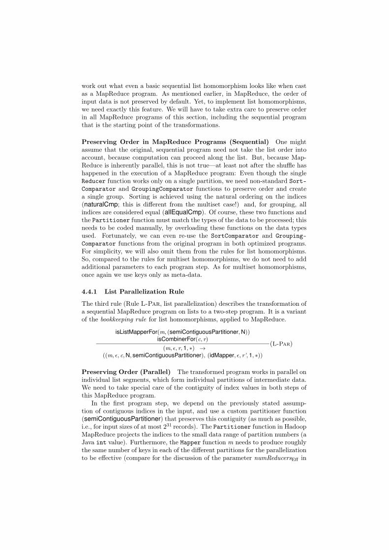
The third rule (Rule L-Par, list parallelization) describes the transformation ofa sequential MapReduce program on lists to a two-step program. It is a variantof the bookkeeping rule for list homomorphisms, applied to MapReduce.

isListMapperFor(m, (semiContiguousPartitioner,N))isCombinerFor(c, r)(m, ε, r, 1, ∗) →

((m, ε, c,N, semiContiguousPartitioner), (idMapper, ε, r’, 1, ∗))

(L-Par)

Preserving Order (Parallel) The transformed program works in parallel onindividual list segments, which form individual partitions of intermediate data.We need to take special care of the contiguity of index values in both steps ofthis MapReduce program.

In the first program step, we depend on the previously stated assump-tion of contiguous indices in the input, and use a custom partitioner function(semiContiguousPartitioner) that preserves this contiguity (as much as possible,i.e., for input sizes of at most 231 records). The Partitioner function in HadoopMapReduce projects the indices to the small data range of partition numbers (aJava int value). Furthermore, the Mapper function m needs to produce roughlythe same number of keys in each of the different partitions for the parallelizationto be effective (compare for the discussion of the parameter numReducersEff in

the cost model, Section 3.3.1). We combine all these constraints into the fol-lowing condition: isListMapperFor(m, (semiContiguousPartitioner, N)).

In the second program step, the input data have no longer contiguous indices,because all values of one partition have been combined into a single value, with asingle index as the key, leaving a gap between subsequent indices. As mentionedpreviously, we could resort to transforming indices to ranges, either directly inthe first Mapper function (m), incurring an additional overhead of around 20%for storing and transferring six instead of five numeric values per record, or in thefirst Reducer function (c), which would then no longer be a Combiner function.We have opted for another solution: We continue working with indices, andaccept that we will not be able to detect errors (that is, intermediate data in anincorrect order) in a fail-fast manner, but only at the end of the computation.This means that, in the second Reducer function (r’ ), we reduce any valueswith strictly increasing indices, and we can only detect (programming) errorswhen there are duplicate or decreasing indices. Put simply, we perform a relaxedcheck on the indices.

Input and Output Programs The input program (left of the arrow) ofRule L-Par consists of one program step. It has variable Mapper (m) andReducer functions (r), no Combiner function, uses a single Reducer task (1)and any partitioner function. The output program is a two-step MapReduceprogram, with a parallel first step (N) and a sequential second step (1). Like theinput program, it does not use Combiner functions. It is parameterized with theMapper function (m) of the original program, a Combiner (c) function used as aReducer function, and a second Reducer function (r’ ), as described above. Inthe second step, it uses an identity function as the Mapper function (idMapper).We could also use the oneKeyMapper function here, that we introduced inRule M-Par, with the advantages of not having to store a key for each record,and of more flexibility in the Mapper function of the original program, but weprefer to pursue an alternative approach that spares us one rule condition. Onceagain, because the second step is sequential, any Partitioner function can beused (∗).

Additional Rule Conditions In addition to constraint isListMapperFor de-scribed above, this rule is only applicable if the Reducer functions c and r arein relation isCombinerFor, that is, if the first Reducer function c is a Combinerfunction compatible with the second Reducer function r.

Cost The cost estimates are very much the same here, for ordered (list) data,as those for unordered (multiset) data, except for two small differences. Onedifference is the extra sorting step necessary to guarantee preservation of order.Although the data are almost sorted (as they consist of a comparably smallnumber of sorted chunks), they need to undergo the complete process of ex-ternal sorting with multiple reads and writes to disk. There seems to be someopportunity for optimization in the Hadoop framework here. Yet, this work isalso needed to achieve grouping alone, and so there is no difference to the casefor multisets. The second difference concerns the type of data processed. Inthe multiset case, we do not need to store anything in the keys of intermediatedata whereas, in the list case, we have chosen to store unique (and contiguous)

list indices. Consequently, we incur more overhead during I/O and comparison.But the additional overhead is present in both list programs, before and afterapplication of Rule L-Par, so there is no difference compared to Rule M-Parfor multisets: We expect the same best and worse cases and, for real programs,we can expect to attain a cost reduction by a factor of between numReducers

2 andnumReducers via Rule L-Par.

4.4.2 List Combiner Rule

The fourth rule (Rule L-Comb, list Combiner) describes the transformationof a two-step MapReduce program on lists to a single-step program that usesa custom Combiner function that is run exactly once. In this rule, the twosteps of the original program together implement a global, ordered reductionin MapReduce (whereas the first step alone implements a segmented, orderedreduction).

isListMapperFor(m, (semiContiguousPartitioner,N))isMapperWithCombinerOnceFor(mc1, (m, c”)) isCombinerFor(c, r)

((m, ε, c,N, semiContiguousPartitioner), (idMapper, ε, r’, 1, ∗)) →(mc1, ε, r’, 1, ∗)

(L-Comb)

Hadoop Combiner Function The idea of Rule L-Comb is, once again, tospeed up processing using a Combiner function. Unfortunately, we cannot useHadoop Combiner functions on list data for three reasons that are caused by rea-sonable design choices in distributed programming. First, to be able to reducethe volume of intermediate data as much as possible, Hadoop applies Combinerfunctions arbitrarily often; thus, they must be idempotent. This is problem-atic because our Combiner function does not preserve the contiguity it requires,and an alternative Combiner function that preserves contiguity by transformingindices to ranges is not idempotent either. Second, to keep the implemen-tation simple and fast, Hadoop Combiner functions are applied to arbitrarysubsets of intermediate data; this,they must be associative-commutative. Thismeans that non-contiguous values will occur frequently, rendering the Combinerfunction almost useless. Third, Hadoop prioritizes sorting over combining, soCombiner functions are only applied to groups of values that are equal accordingto GroupingComparator and also SortComparator—and, for sorting, we needgroups of single values, which cannot be combined, rendering the Combinerfunction a no-op.

Preserving Order (Optimized Parallel) As a resort, we use a custom-built function (mc1 ). It is a Mapper function that also executes the logic ofa Combiner function, but only once, on the complete list of intermediate val-ues produced by the Mapper, and in the order in which they have been produced.This requirement is expressed by relation isMapperWithCombinerOnceFor, whichis parameterized with the new Mapper function mc1 and the defining Mapperand Combiner functions (here, m and c”). For our experiments (Section 5), wehave implemented this by refactoring the Combiner code, thereby adding a newfunction that can perform the reduction in a streaming fashion, and we call thisfunction from the Mapper code for each new intermediate value produced. This

eliminates problems with memory management (the worry of whether the inter-mediate values fit into the memory assigned to the Mapper task), and it does notrequire a reimplementation of the rather complicated interface between Mapperand Combiner functions (a read-once iterator reusing mutable singleton con-tainers for possibly serialized keys and values, grouped by some function).

Variables Rule L-Comb is parameterized with two different Mapper functions(m, mc1 ), and different variants of Combiner (c, c”) and Reducer functions (r,r’ ). The difference between the Reducer functions is that function r’ onlyperforms a relaxed check, as described above; the Combiner function c” doesnot perform any check at all.

Input and Output Programs The input program is a two-step MapReduceprogram. It uses the functions idMapper and semiContiguousPartitioner de-scribed above. More precisely, it is of the form produced by Rule L-Par. Theresulting program is single-step. It uses the custom-built function mc1 as itsMapper function, no Hadoop Combiner function (as explained above), the re-laxed Reducer function r’, any Partitioner function, and it has only a singleReducer (1; no parallelism here). All parallelism is associated with functionmc1.

Additional Rule Conditions isListMapperFor and isCombinerFor are thesame as in Rule L-Par, with the same parameters as mentioned there; concern-ing the relation isMapperWithCombinerOnceFor, see the explication on pre-serving order given above.

Cost All arguments that we have given for Rule M-Comb also hold for Rule L-Comb. So, we expect a speedup of slightly more than a factor of 2 for mostpractical problem sizes.

5 ExperimentsSo far, we have developed a lot of theory: We have started with a functionalmodel of MapReduce, continued with a cost model, and finished with four op-timization rules—-two rules for each of two classes of programs, resemblingmultiset and list homomorphisms.

We do not prove the correctness of these rules formally, an approach othershave pursued [16]. Instead, we will take an experimental approach to demon-strate their practicality.

5.1 Research QuestionWe consider Hadoop Java programs and perform tests to measure performanceand speedup. Our research question is: “Do the optimization rules achieve theindicated performance gain?” So, we report on an exploratory evaluation of theoptimization rules in this section. Our conclusion is that the results justify theformal model, on which the rules are based.

5.2 Experimental SetupIn the following, we describe the code of the Hadoop MapReduce programs thatwe have implemented. First, we describe briefly the Java interface to Hadoopthat we developed to resemble our functional model. Then, we proceed with theexample programs for two problems to which we apply the optimization rules.

5.2.1 Java MapReduce Skeleton

Hadoop MapReduce programs are meta-programs that make heavy use of Javareflection. In particular, the semantics and the type of result data depend ona numeric parameter (called numReducers in the cost model). When portingthe formal model of MapReduce (in Section 3.1) from Haskell to Java withGenerics, we needed to create two Java instances to enable type checking: onewith a Hadoop Combiner function and one without.9 In Java, we do representthe key–value pairs that we have abstracted away in the functional model. Theyare modelled as separate keys and values, forgoing the notion of being part ofa pair. So, the Mapper function parameter in our formal model (Section 3.1)with Haskell type m -> [r] becomes an object parameter of our Java skeleton,which takes the form of a Java function; the object needs to be an instanceof the generic Hadoop class Mapper<K1,V1, K2,V2>, where K1 and V1 are theJava types of the keys and values in the input type m, and K2 and V2 are theJava types of the keys and values in the result type r (the list in the result type[r] is not represented explicitly). When passed to Hadoop, the Mapper functionparameter will have the even less expressive reflective type of Class<? extendsMapper>. In both instances of the Java skeleton, parameter numReducers isalso passed on to Hadoop. Furthermore, we pass on some more type parametersneeded by Hadoop for (de)serialization. Lastly, we use Hadoop’s Partitionerfunction on keys and values instead of a third comparator. Apart from this,the two resulting Java skeletons are straightforward adaptations of our Haskellskeleton. More information on the Java skeletons are available in Appendix Aas well as in Doerre et al. [17].

5.2.2 Subject Programs

For each of the two pairs of optimization rules, we created an example programfrom the class of programs to which the first rule of the pair applies, optimized itaccording to this rule, and optimized it further using the second rule of the pair.This enables us to assess the performance of the original and the transformedprograms. Thus, for both multiset and list homomorphisms, we have threeprogram variants of an example program each.

Sequential: the original, unoptimized program, using one Hadoop programstep; the baseline variant

TwoStep: the program after application of the corresponding parallelizationrule (Rule M-Par or L-Par), using two Hadoop program steps; no Combinerfunction

9Two additional instances will be needed to support MapReduce programs without aReducer function

Optimized: the final program after also applying the corresponding Combinerrule (Rule M-Comb or L-Comb), using one Hadoop program step; asuitable Combiner function

Multiset Homomorphism: Maximum We will first apply the optimizationrules on multisets to the Maximum (Max) problem. The problem consists offinding the maximum value in a list of signed 32-bit Java int values. Thisproblem represents a whole set of database aggregation operators, for example,count, sum, and average (i.e., it can be easily modified to implement theseoperators). Because the binary operator max is associative and commutative,Max is a multiset homomorphism.

Given the Java MapReduce skeleton for Hadoop, it is now straightforwardto implement the Sequential Maximum problem in Hadoop, and to derive theTwoStep and the Optimized variant using the optimization rules stated in Sec-tion 4.3. Each of them makes use of the same user-defined Reducer functionthat implements a max computation on a list (or, more exactly, on an iterator)of intermediate values. Note that, for Maximum, the optimized parallel Map-Reduce program is known and easy to write without this method. This exampleis mainly used as an intermediate step to the more complex Maximum SegmentSum problem that follows.

List Homomorphism: Maximum Segment Sum Our next example isthe Maximum Segment Sum (MSS) problem, which is defined as follows: Foran input list of integers, look at each segment (a sublist containing only consec-utive list elements), and compute its sum; return the maximum of these sums.We have selected MSS for several reasons: It works on lists, it is non-trivial toparallelize, using a complex operator on intermediate data and post-processing,and it has been studied extensively in parallel functional programming [6]. Nev-ertheless, MSS is grounded in a practical use case: Its original two-dimensionalformulation was intended to be used as a simplified maximum likelyhood es-timator on digital images [4]. A naïve implementation of this algorithm is ofcubic time complexity. Optimal sequential implementations have linear timecomplexity and run in a streaming fashion (as a linear scan), requiring onlyconstant space at any time. The algorithm described next will also have theseproperties when run sequentially. Nevertheless, we are concerned with paral-lel implementations here. MSS is both an instance of the divide-and-conquerprogram skeleton and a list homomorphism [6].

As with the Maximum problem, we have created three different MapReduceimplementations of MSS. More information on the subject programs are avail-able in Appendix B.

5.2.3 Test Input Data

Now that we have described the test programs, let us describe the test inputdata which they process.

Format The test input data are made up of random 32-bit signed integervalues. For consistency, we use the same input data for both problems in theevaluation. This means that, although this is only needed for list homomor-phisms, all input records also contain the current (32-bit signed integer) index

in the key part of a key–value pair. For ease of access, each input record isstored as the textual representation of the key and the textual representationof the value, separated by a tab and terminated by a newline.

Scaling Because Hadoop is optimized for larger files, we start testing with asize of 16 million (224) input records (see parameter chunkSize of our cost model,described in Section 3.3.1). We double the input size between consecutive tests,which gives us an evenly-spaced doubly-logarithmic scale. Technically, we re-usethe input file(s) of the smaller size and add the same number of input files ofsize 224 records each to reach the next (binary) order of magnitude. We stop at231 input records for two reasons. First, disk space and run time do not allowfor much bigger inputs, given the cluster on which we run our experiments, asdescribed in Section 5.3.1. Second, and more importantly, the return type ofthe Java Object’s hashCode method is a 32-bit signed integer (a Java int). Itis used pervasively by the Hadoop MapReduce framework for partitioning andcannot be changed easily to a bigger type. We depend on this functionalitywhen preserving order for list homomorphisms and, for consistency, we use thesame input sizes also for multiset homomorphisms.

5.3 ExperimentsNext, we describe the experiments performed, to quantify the performance gainsobtainable using the optimization rules.

5.3.1 Measurement Setup

The measurement environment consists of hardware, software, and measurementtools.

Hardware All experiments were run on the same 16-node cluster (which hasone additional master node with a similar configuration); the input was dis-tributed across the cluster (in the Hadoop distributed file system); each nodehas

• 2 ∗ 4 CPU cores (Intel(R) Xeon(R) CPU E5405 @ 2.00GHz)

• 16 GB of RAM (plus 8 GB of swap space on hard disk)

• 1 hard disk volume (striped on 2 ∗ 72 GB physical disks; one node has2 ∗ 600 GB)

• 1 GBit Ethernet, connected through a switch

In total, there are 16 ∗ 2 ∗ 4 = 128 CPU cores in the cluster. In the optimalcase, CPU-bound programs that can run fully parallel will be able to makeuse of this degree of parallelism. Any additional speedup is likely due to cacheeffects.

Third-Party Software The operating system was a 64-bit openSUSE 10.3Linux (kernel 2.6.22.17-0.1-default). The Java Virtual Machine (from Ora-cle) was: Java(TM) SE Runtime Environment (build 1.6.0_15-b03) with JavaHotSpot(TM) 64-Bit Server VM (build 14.1-b02, mixed mode).

Hadoop Configuration With the given data encoding, inputSize is 310MBfor each file of 224 records. Given the chunkSize of 64MB, this amounts to 6input splits per input file. We have verified that the outputSize for all programsis a very small constant (some dozen bytes). We used a replication factor of 2in the Hadoop DFS. In Hadoop MapReduce, we used at maximum 8 Mappertasks and 8 Reducer tasks per 8-core cluster node, allowing for potentially fullutilization in all phases, even if only Mapper or only Reducer tasks are at work.Following standard guidelines [numReducers in Hadoop Wiki], in all parallelprogram steps, we used 111 Reducer tasks (which is slightly less than the numberof CPU cores).

Measuring Runtime We used the tool GNU time 1.7 to measure the wall-clock run time, including startup overheads of the user program. The serverprocesses on each cluster node ran for weeks, and the Java just-in-time compilerand the data caches have been warmed up with the real input data for bothprograms before the measurements start for each input size. We only measuredeach point once, because the small measurement differences that occurr havelittle influence on the trends that we expected to observe and compare.

5.3.2 Performance Results

In the Figures 3 and 4, we show, for both the Max and the MSS problem, theperformance of the original program and the program after applying only thefirst and both optimization rules, respectively.

For both problems, we used the same setup. The results are plotted on adoubly-logarithmic scale. On the horizontal axis, we have the binary (or dyadic)logarithm of the number of elements in the input, as described in Section 5.2.3;it starts at 224, because this is the minimum number of input records. Thevertical axis records the binary logarithm of the program run time in seconds,as just described. The raw results are also shown in Table 1.

24 25 26 27 28 29 30 31

02

46

81

01

2

input size: log2(records)

run tim

e: lo

g2(s

econds)

● ● ● ● ●

●

●

●

Max problem

●Sequential TwoStep Optimized

Figure 3: Wall-clock run time of the Sequential, TwoStep, Optimized programsfor the Max problem on input sizes between 224 and 231 records.

Max Problem For the Max problem, the TwoStep program is much fasterthan the Sequential program for large inputs (by a factor of 24.2), and the

24 25 26 27 28 29 30 31

02

46

81

01

2

input size: log2(records)

run tim

e: lo

g2(s

econds)

● ● ● ● ●

●

●

●

MSS problem

●Sequential TwoStep Optimized

Figure 4: Wall-clock run time of the Sequential, TwoStep, Optimized programsfor the MSS problem on input sizes between 224 and 231 records.

Optimized program is even faster for all inputs (up to a factor of 25.2 comparedto the Sequential program).

MSS Problem For the MSS problem, the TwoStep program is orders of mag-nitude faster than the Sequential program for medium and large inputs (up toa factor of 24.8), and the Optimized program is even faster for all inputs (up toa factor of 26.4).

Raw data Table 1 shows the raw data for Figure 3 and Figure 4, again asdoubly-logarithmic values. The run time for input sizes between 224 and 231

records is shown in log2 seconds.

5.4 DiscussionNext, we discuss the performance gains obtained by applying the optimizationrules, and the consequences for both the functional and the cost model.

Table 1: Raw data (log2 of wall-clock run time in seconds) of the Sequential,TwoStep, Optimized programs for both the Max and the MSS problem on inputsizes between 224 and 231 records.

Max MSS

log2 records Optimized TwoStep Sequential Optimized TwoStep Sequential

24 5.07 6.48 5.50 5.06 6.55 6.1825 5.07 6.48 5.70 5.06 6.52 6.4826 5.07 6.48 6.40 5.06 6.56 7.4227 5.16 6.50 7.38 5.08 6.57 8.4828 5.24 6.41 8.52 5.15 6.59 9.4929 5.79 6.86 9.76 5.70 7.06 11.1930 6.32 7.37 11.11 6.09 7.61 12.2731 7.05 8.04 12.25 6.88 8.44 13.28

Performance Overall, the results for the optimization of the Max and MSSproblems are very similar. The biggest difference is that Max is up to twiceas fast as MSS, especially when comparing the Sequential variants for the twoproblems. So, let us discuss them together. Looking at the diagrams, the Se-quential variants take very long for larger input sizes (more than 228 records);the TwoStep variants are much faster and the Optimized variants are the fastestby some factor of 2. For smaller input sizes (224 to 228 records), the executiontimes of the non-sequential variants do not depend on the input size, but are con-stant; this can be explained by the dominance of the startup overhead. For evensmaller input sizes, this is likely to apply also to the Sequential variants. TheTwoStep variants take around three times as long as the Optimized variants—except for the Max program with large inputs, in which case the slowdown factoris 2, not 3.

Speedup Compared to the Sequential variant, the speedup of the TwoStepprogram for the Max problem grows from 2−1 to 24.2 with an increase of afactor of 27 in input size (from 224 to 231 records), and the speedup of theOptimized program grows from 20.4 to 25.2 in the same frame. Likewise, for theMSS problem, the TwoStep program shows a speedup of between 2−0.4 and 24.8

(with a slightly different slope), and the Optimized program exhibits a speedupof between 21.1 and 26.4 (which is a speedup of around 85).

Interpretation The observed speedups are not unexpected. In Section 4,we describe the cost reduction associated with each optimization rule. Thesecosts ranged from a slowdown by a factor of 2 (as exhibited by the TwoStepprogram variant of the Max problem on the smallest input size) to a speedup of2 ∗ numReducers ≈ 2 ∗ 128 = 256 = 28 (theoretically, if the best cases of bothrules apply to the same input size; we observed 26.4 for the Optimized programvariant of the MSS problem on the biggest input size). The data points betweenthese extreme values also align well with our expectations.

Justification We have chosen a formal and algebraic approach to explore thepossibilities of MapReduce program optimizations. Our approach has the ad-vantage of being both better founded and able to give more practical advice thanthe current best practice for MapReduce program development, namely, rulesof thumb as, for example, the following one, taken from the introduction of theHadoop documentation: If your program is slow, try to use a Combiner func-tion. We had to apply several simplifications in the functional and cost modeland the optimization rules compared to the practical evaluation using Hadoop.We have already discussed the performance-related points in Section 3.2, Sec-tion 3.3.3 and Section 4.2. Nevertheless, the optimization rules worked. This isbecause, at least, for the problem classes described, the models seem to matchthe Hadoop programs well.

Recommendation of Use For all but trivially small input sizes, the paral-lelization sule M-Par and L-Par should be applied to MapReduce programs.Concerning the combiner rules M-Comb and L-Comb, the situation is lessclear: The performance gain alone (a factor of 2 or 3) may not pay off, given the

development effort needed to implement it. But, the target program has the ex-tra benefit of expressing a one-step computation (in the logical/homomorphismview) by a one-step program (instead of two separate MapReduce steps). Thisis more intuitive, and it renders operations more manageable.

Further Applications We have demonstrated that our functional model andour cost model are useful and principled tools for formulating and reasoningabout performance optimization of MapReduce programs. Beyond formulat-ing further optimizations, the models can serve as a basis for reasoning aboutproperties other than performance. First, the functional model can be a foun-dation for modeling and reasoning about functional correctness of MapReduceprograms and their optimizations. Second, the cost model can be extended tocover also other non-functional properties, such as reliability and energy con-sumption. Overall, a formal approach to this domain—as taken by us—will helpto classify, compare, inspire, and guide further work on MapReduce program-ming and similar models for distributed programming.

6 Related WorkSince its invention, a huge amount of research has been conducted on HadoopMapReduce optimization [9]. Yang et al. [18] state the main principles andrequirements of MapReduce implementations.

The authors of MapReduce themselves recommend that one should takeadvantage of natural indices whenever possible [8]. This supports our interest inlist homomorphisms, in which order plays an important role. Map-Join-Reduceextends MapReduce by user-specified join functions that allow to control theorder or items during joining [19].

HaLoop optimizes the execution of MapReduce programs by caching in-termediate results between MapReduce jobs [20]. This is an alternative toour approach of merging jobs structurally based on our model. Similarly toHaLoop, iMapReduce also optimizes the execution of MapReduce programs,not by caching, but by pooling and reusing suspended MapReduce jobs [21].

The MRShare system transforms a batch of queries into a new batch bymerging jobs into groups and an evaluating each group as a singlen query [22].The transformation is based on a cost model. Again, this is not really a struc-tural program rewrite, as we do it.

Babu [23] introduces a profiler that monitors, based on instrumentation, theexecution of a Hadoop MapReduce program, and a cost-based optimizer thattunes the underlying parameters of the Hadoop framework. This is parametertuning, which is complementary to our approach of a structural program opti-mization. Similarly, Herodotou et al. [24, 25, 26] perform parameter tuning, inthis case, based on clustering.

The Manimal system performs a static analysis to determine relational op-timizations and to generate proper indexes for the raw data [27, 28], no archi-tectural optimization, as we do it.

Several approached concentrate on increasing fault tolerance, mostly by mon-itoring and job re-scheduling: ParaTimer [29, 30], LATE [31], RAFT [32, 33]and Hadoop++ [34]. Several systems perform optimization on logical query

plans, much like in ordinary databases: FlumeJava [35], Pig Latin [36] andTenzing [37].

Finally, some tools provide declarative interfaces to Hadoop, but these arerather SQL-like data processing interfaces, and not architectural models likeours: Sawzall [38], Pig Latin [36], Tenzing [37], Hive [39] and SQL/MapReduce[40].

7 Conclusions and Future WorkGoogle’s MapReduce programming model has been one of the contributionswith highest practical impact in the field of distributed computing in the re-cent year. It is closely related to functional programming, especially to thealgebraic theory of list homomorphisms. List homomorphisms facilitate pro-gram composition, optimization of intermediate data, and parallelization. Toput these theoretical benefits to practical use, we strive for a combination of theformal basis of list homomorphisms with the scalability and industrial-strengthdistributed implementation of MapReduce.

In particular, we have developed a formal model of MapReduce programssuitable for optimization (comprising a functional model and a cost model),an approach to write MapReduce programs that operate on lists instead ofon multisets only, a total of four optimization rules for MapReduce programsformulated on top of our formal model, and a series of experiments to validatethe model and the optimization rules.

We believe that the development of MapReduce programs, for example usingHadoop, benefits from the use of a formal functional model and cost model. Ourwork is a first step on the way to easier MapReduce programming.

There are several avenues that can be followed in the future. First, onecan conduct a complete, controlled experimental evaluation as a follow-up ofthe exploratory evaluation reported on here. Second, one can try to extend or,even better, further simplify the (cost) model, and to mechanize it in the formof an automatic optimizer for (certain) MapReduce programs. Third, one cangeneralize the findings beyond the (Hadoop) MapReduce context.

8 AcknowledgementsThis work received financial support under DFG project MapReduceFoundation,grant no. Le 912/13-1.

References[1] Sterling TL, Savarese D, Becker DJ, Dorband JE, Ranawake UA, Packer

CV. BEOWULF: A parallel workstation for scientific computation. Proc.Int. Conf. on Parallel Processing (ICPP), vol. 1, CRC Press, 1995; 11–14.2

[2] Dean J, Ghemawat S. MapReduce: Simplified data processing on largeclusters. Proc. 6th Symp. on Operating Systems Design and Implementation(OSDI), USENIX Association, 2004; 137–150. 2, 5, 6, 23

[3] White T. Hadoop: The Definitive Guide. 3rd edn., O’Reilly, 2012. 4, 6

[4] Bentley J. Programming pearls: Algorithm design techniques. Comm.ACM 1984; 27(9):865–873. 4, 31

[5] Bird R. Algebraic identities for program calculation. Computer J. 1989;32(2):122–126. 4

[6] Gorlatch S. Toward formally-based design of message passing programs.IEEE Trans. on Software Engineering (TSE) 2000; 26(3):276–288. 4, 31

[7] Dean J, Ghemawat S. MapReduce: Simplified data processing on largeclusters. Comm. ACM 2008; 51(1):107–113. 5, 9, 14, 23

[8] Dean J. MapReduce: A flexible data processing tool. Comm. ACM 2010;53(1):72–77. 5, 23, 36

[9] Sakr S, Liu A, Fayoumi AG. The family of MapReduce and large-scale dataprocessing systems. ACM Comp. Surveys Oct 2013; 46(1):44 pp. Article11. 5, 36

[10] Bird R. Lectures on constructive functional programming. Technical Re-port PRG-69, Programming Research Group, Oxford University Comput-ing Laboratory Sep 1988. 9

[11] Lämmel R. Google’s MapReduce programming model – Revisited. Scienceof Computer Programming (SCP) Jan 2008; 70(1):1–30. 9, 23

[12] Forum MPI. MPI: A Message Passing Interface Standard, Version 2.1.High-Performance Computing Center Stuttgart, 2008. 9

[13] Gorlatch S. Systematic efficient parallelization of scan and other list homo-morphisms. Euro-Par’96: Parallel Processing, Vol. II, Bougé L, FraigniaudP, Mignotte A, Robert Y (eds.), LNCS 1124, Springer-Verlag, 1996; 401–408. 9

[14] Marlow S ( (ed.)). Haskell 2010 Language Report. haskell.org, 2010. URLhttp://www.haskell.org/onlinereport/haskell2010/. 10

[15] Bird R. Introduction to Functional Programming using Haskell. 2nd edn.,Prentice Hall Series in Computer Science, Prentice Hall Europe, 1998. 22

[16] Ono K, Hirai Y, Tanabe Y, Noda N, Hagiya M. Using Coq in specificationand program extraction of Hadoop MapReduce applications. Software En-gineering and Formal Methods (SEFM), Barthe G, Pardo A, Schneider G(eds.), LNCS 7041, Springer, 2011; 350–365. 29

[17] Dörre J, Apel S, Lengauer C. Static type checking of Hadoop MapReduceprograms. Proc. Int. Workshop on MapReduce and its Applications (Map-Reduce), ACM Press, 2011; 17–24. 30, 41

[18] Yang HC, Dasdan A, Hsiao RL, Parker DS. Map-reduce-merge: Simplifiedrelational data processing on large clusters. Proc. ACM SIGMOD Int. Conf.on Management of Data (SIGMOD), ACM, 2007; 1029–1040. 36

[19] Jiang D, Tung AKH, Chen G. MAP-JOIN-REDUCE: Toward scalable andefficient data analysis on large clusters. IEEE Trans. on Knowl. and DataEng. Sep 2011; 23(9):1299–1311. 36

[20] Bu Y, Howe B, Balazinska M, Ernst MD. HaLoop: Efficient iterative dataprocessing on large clusters. Proc. VLDB Endow. Sep 2010; 3(1–2):285–296. 36

[21] Zhang Y, Gao Q, Gao L, Wang C. iMapReduce: A distributed computingframework for iterative computation. J. Grid Comput. Mar 2012; 10(1):47–68. 36

[22] Nykiel T, Potamias M, Mishra C, Kollios G, Koudas N. MRShare: Sharingacross multiple queries in MapReduce. Proc. VLDB Endow. Sep 2010; 3(1–2):494–505. 36

[23] Babu S. Towards automatic optimization of MapReduce programs. Proc.1st ACM Symp. on Cloud Computing (SoCC), ACM, 2010; 137–142. 36

[24] Herodotou H, Babu S. Profiling, what-if analsyis, and cost-based optimiza-tion of MapReduce programs. Proc. VLDB Endow. 2011; 4(11):1111–1122.36

[25] Herodotou H, Dong F, Babu S. MapReduce programming and cost-basedoptimization? crossing this chasm with a starfish. Proc. VLDB Endow.2011; 4(12):1446–1449. 36

[26] Herodotou H, Lim H, Luo G, Borisov N, Dong L, Cetin FB, Babu S.Starfish: A self-tuning system for big data analytics. Proc. 5th Bienn. Conf.on Innovative Data Systems Research (CIDR), 2011; 261–272. 36

[27] Cafarella MJ, Ré C. Manimal: Relational optimization for data-intensiveprograms. Proc. 13th Int. Workshop on the Web and Databases (WebDB),ACM, 2010; 10:1–10:6. 36

[28] Jahani E, Cafarella MJ, Ré C. Automatic optimization for MapReduceprograms. Proc. VLDB Endow. Mar 2011; 4(6):385–396. 36

[29] Morton K, Balazinska M, Grossman D. ParaTimer: A progress indicatorfor MapReduce DAGs. Proc. ACM SIGMOD Int. Conf. on Managementof Data (SIGMOD), ACM, 2010; 507–518. 36

[30] Morton K, Friesen A, Balazinska M, Grossman D. Estimating the progressof MapReduce pipelines. Proc. IEEE 29th Int. Conf. on Data Engineering(ICDE), IEEE Computer Society, 2010; 681–684. 36

[31] Zaharia M, Konwinski A, Joseph AD, Katz R, Stoica I. Improving Map-Reduce performance in heterogeneous environments. Proc. 8th USENIXConf. on Operating Systems Design and Implementation (OSDI), USENIXAssociation, 2008; 29–42. 36

[32] Quiané-Ruiz JA, Pinkel C, Schad J, Dittrich J. RAFTing MapReduce: Fastrecovery on the RAFT. Proc. 27th Int. Conf. on Data Engineering (ICDE),IEEE Computer Society, 2011; 589–600. 36

[33] Quiané-Ruiz JA, Pinkel C, Schad J, Dittrich J. RAFT at work: Speeding-up MapReduce applications under task and node failures. Proc. ACM SIG-MOD Int. Conf. on Management of Data (SIGMOD), ACM, 2011; 1225–1228. 36

[34] Dittrich J, Quiané-Ruiz JA, Jindal A, Kargin Y, Setty V, Schad J.Hadoop++: Making a yellow elephant run like a cheetah (without it evennoticing). Proc. VLDB Endow. Sep 2010; 3(1–2):515–529. 36

[35] Chambers C, Raniwala A, Perry F, Adams S, Henry RR, Bradshaw R,Weizenbaum N. FlumeJava: Easy, efficient data-parallel pipelines. Proc.ACM SIGPLAN Conf. on Programming Language Design and Implemen-tation (PLDI), ACM, 2010; 363–375. 37

[36] Olston C, Reed B, Srivastava U, Kumar R, Tomkins A. Pig Latin: A not-so-foreign language for data processing. Proc. ACM SIGMOD Int. Conf.on Management of data (SIGMOD), ACM, 2008; 1099–1110. 37

[37] Chattopadhyay B, Lin L, Liu W, Mittal S, Aragonda P, Lychagina V, KwonY, Wong M. Tenzing A SQL implementation on the MapReduce framework.Proc. VLDB Endow. Aug 2011; 4(12):1318–1327. 37

[38] Pike R, Dorward S, Griesemer R, Quinlan S. Interpreting the data: Parallelanalysis with Sawzall. Sci. Program. Oct 2005; 13(4):277–298. 37

[39] Thusoo A, Sarma JS, Jain N, Shao Z, Chakka P, Anthony S, Liu H, WyckoffP, Murthy R. Hive – A warehousing solution over a Map-Reduce framework.Proc. VLDB Endow. Aug 2009; 2(2):1626–1629. 37

[40] Friedman E, Pawlowski PM, Cieslewicz J. SQL/MapReduce: A practicalapproach to self-describing, polymorphic, and parallelizable user-definedfunctions. Proc. VLDB Endow. Aug 2009; 2(2):1402–1413. 37

A Java Skeleton for Hadoop MapReduceIn this section, we provide more detail of the Java incarnation of our functionalmodel. We pay special attention to the typing issues that arise because of theuse of generic types in Java, in continuation of our work on improved statictyping for MapReduce programs [17].

On the implementation side, we use Java and Hadoop for our example Map-Reduce programs. In our functional model (Section 3.1), we have extracted themost important parameters from the many parameters that Hadoop and otherMapReduce frameworks accept. If we port the functional model to Java, theresult is a Java program skeleton that is very similar to our Haskell programskeleton of MapReduce. The main difference is that, on the Java side, becauseof the pervasive use of reflection in Hadoop, we really have a meta-program withmore flexibility than we could attain in plain Haskell. This flexibility allows usto introduce an additional parameter (a natural number) that specifies exactlythe number of Reducer tasks to run. (We have already used this parameter inthe cost model and in the optimization rules.) There are three possible kinds ofbehavior and associated (Java) types of result data depending on the value ofthis numeric parameter.

• With zero Reducer tasks, only the Mapper function is run. The user-defined Partitioner, SortComparator, GroupingComparator, Combiner,and Reducer functions are not used. Consequently, the user-defined typeof the final output data is given by the return type of the Mapper function,and not by the return type of the Reducer function, as would normally bethe case.

• With one Reducer task, any Partitioner specified produces only a singlepartition. Thus, the single Reducer task processes all intermediate data,and it has a global view of this data.

• With any larger number of Reducer tasks, everything happens as normal(as described in Section 2.1).

The types in last two cases can be unified, regarding a single result as a singletonlist, but the MapReduce program skeleton still has two different possible resulttypes.

No Compile-Time Checks Of course, the flexibility of selecting differentbehaviors, via a numeric value at run time, comes at a price. For example, unlikein Haskell (the programming language of our functional model), two MapReduceprograms using the Java skeleton cannot be composed in a type-safe manner,because they are not fully type-checked until run time. One would need to takethe number of Reducer tasks specified into account to be able to decide betweenthe two possible result types of the first MapReduce program, and to verify typecorrectness. Of course, this would be possible using an external type checker;yet, in our current implementation, this is impossible to achieve at compile time,because there is only a thin wrapper library around the Hadoop Java API thatuses the standard Java type-checker and its support for generics. The best wecould do is to provide a separate skeleton for the case of zero Reducer tasks,and to throw a run-time error if the user specifies a zero value in the normal

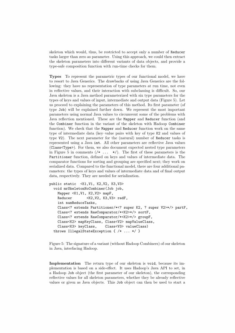
skeleton which would, thus, be restricted to accept only a number of Reducertasks larger than zero as parameter. Using this approach, we could then extractthe skeleton parameters into different variants of data objects, and provide atype-safe composition function with run-time checks for them.

Types To represent the parametric types of our functional model, we haveto resort to Java Generics. The drawbacks of using Java Generics are the fol-lowing: they have no representation of type parameters at run time, not evenin reflective values, and their interaction with subclassing is difficult. So, ourJava skeleton is a Java method parameterized with six type parameters for thetypes of keys and values of input, intermediate and output data (Figure 5). Letus proceed to explaining the parameters of this method. Its first parameter (oftype Job) will be explained further down. We represent the most importantparameters using normal Java values to circumvent some of the problems withJava reflection mentioned. These are the Mapper and Reducer function (andthe Combiner function in the variant of the skeleton with Hadoop Combinerfunction). We check that the Mapper and Reducer function work on the sametype of intermediate data (key–value pairs with key of type K2 and values oftype V2). The next parameter for the (natural) number of Reducer tasks isrepresented using a Java int. All other parameters are reflective Java values(Class<Type>). For them, we also document expected nested type parametersin Figure 5 in comments (/* ... */). The first of these parameters is thePartitioner function, defined on keys and values of intermediate data. Thecomparator functions for sorting and grouping are specified next; they work onserialized data. Compared to the functional model, there are four additional pa-rameters: the types of keys and values of intermediate data and of final outputdata, respectively. They are needed for serialization.

public static <K1,V1, K2,V2, K3,V3>void mrSkeletonNoCombiner(Job job,

Mapper <K1,V1, K2,V2> mapF,Reducer <K2,V2, K3,V3> redF,int numReduceTasks,Class<? extends Partitioner/*<? super K2, ? super V2>*/> partF,Class<? extends RawComparator/*<K2>*/> sortF,Class<? extends RawComparator/*<K2>*/> groupF,Class<K2> mapKeyClass, Class<V2> mapValueClass,Class<K3> keyClass, Class<V3> valueClass)

throws IllegalStateException { /* ... */ }

Figure 5: The signature of a variant (without Hadoop Combiners) of our skeletonin Java, interfacing Hadoop.

Implementation The return type of our skeleton is void, because its im-plementation is based on a side-effect. It uses Hadoop’s Java API to set, ina Hadoop Job object (the first parameter of our skeleton), the correspondingreflective values for all skeleton parameters, whether they be already reflectivevalues or given as Java objects. This Job object can then be used to start a

distributed Hadoop job. (As an aside: a job already running cannot be config-ured any further, which leads to the IllegalStateException mentioned in thetype.)

In Figure 6, we show a call to this Java skeleton, which is suitable for theSequential variant of the MSS example program. As described before, the firstparameter is the Hadoop Job object to be configured.

public class MssMainIndexedSequential /* ... */ {

Mapper<LongWritable, Text, LongWritable, LongWQuadruple>map = new IndexedTextToLongWQuadrupleValueMapper();

Reducer<LongWritable,LongWQuadruple, LongWritable,LongWQuadruple>reduce = new IndexedMssReducerRelaxed();

mrSkeletonNoCombiner(job,map,reduce,1,HashPartitioner/*<LongWritable,Object>*/

/*<Object,Object>*/.class,NaturalLongWritableComparator.class,AllEqualComparator/*<LongWritable>*/ /*<Object>*/.class,LongWritable.class, LongWQuadruple.class,LongWritable.class, LongWQuadruple.class);

/* ... */}

Figure 6: A call (from the Sequential program for the MSS problem) to the Javaskeleton shown in Figure 5.

We store the Mapper (map) and Reducer (reduce) objects in separate vari-ables make the types that they use explicit. The input (when read by thestandard Hadoop TextInputFormat) consists of the (binary) position offset inthe current input file as the key of type LongWritable, and the textual values ofindex and data item as the value of type Text. These are the first two type pa-rameters of the Mapper object used. The text is then parsed, the index is storedin the intermediate key of type LongWritable, and the data item is stored asa quadruple with four identical entries in the value of type LongWQuadruple.This is needed to apply a homomorphism to the data: we need to store thisadditional information in the intermediate data to be able to re-combine partialresults (for contiguous data) in multiple passes, and even to forgo the need tostore all input data. The Reducer function implements a true reduction on thisintermediate data; in consequence, it produces output of the same type. TheMapper and Reducer objects are the second and third parameters of the Map-Reduce skeleton (in the variant without Hadoop Combiner function), whichguarantees that the types of intermediate data used by Mapper and Reducerfunction coincide. This can be checked by looking at the declarations of mapand reduce. They also need to coincide with the types represented by the Javaclass literals that are the four last parameters of the skeleton (two for interme-

diate keys/values, two for output keys/values). The remaining parameters arethe number of Reducer tasks in a sequential program (1), and the class literalsof the functions for partitioning, sorting, and grouping the type of intermediatedata used.

B Descriptions of Subject ProgramsIn this section, we describe how the optimization rules (Section 4) must beinstantiated for the subject programs used in the experiments (Section 5.2.2).

B.1 Multiset Homomorphism: MaxThe Max problem can be defined using an associative, commutative, binaryreduction operator max (which is the parameter of reduce; see Section 2.4).Commutativity entails that the order of elements in the input list (and also inpossible intermediate result lists) does not matter, so the input can be regardedas a multiset. Furthermore, every reduction can be regarded as a list homo-morphism with the identity function (id), both as the parameter to the mapcombinator and as the post-processing function. Thus, a Haskell implementa-tion of the Max problem might look as follows:

maximum = (id) . reduce(max) . map(id)

Finally, every list homomorphism with a commutative reduction operator is amultiset homomorphism. So, this Haskell implementation of Max is a multisethomomorphism, too.

Max MapReduce Programs Let us now describe three different implemen-tations of Max in MapReduce, and how to get from one to the next, using theoptimization rules stated in Section 4.3.

Sequential There are two variables on the left-hand side of rule M-Par(Section 4.3.1), which have to be instantiated for the Max problem: Mapperfunction m and Reducer function r. The Mapper function m is called on eacha line of the input text file. It splits the line into key and value, discards theunnecessary index in the key, parses the value into a Java long integer, convertsit to a Hadoop LongWritable, and returns it together with a constant key. TheReducer function r iterates over the LongWritable values that are passed to it,converts each value into a Java long integer, reduces all these values using themax function, and finally converts the single result to a Hadoop LongWritableand returns it together with a constant key.

TwoStep We use rule M-Par to create a two-step parallel MapReduceprogram for the Max problem. On the right-hand side of rule M-Par, Reducerfunction r is already bound to the value used on the left-hand side of this rule.The additional variables that need to be instantiated are Mapper function m’and Combiner function c. They are constrained by the relations in the conditionof the rule. The choice of Combiner function c is given by Reducer functionr. Concerning Mapper function m’, there is some freedom in the set to which

the input keys are mapped: we need to map the set of all input keys to a(not too) small set of different intermediate keys. This is because we needa certain number (some hundreds or thousands) of segments, which will beprocessed in parallel. So, we need sufficiently many keys for parallelism in thefirst MapReduce program step and, at the same time, not too many groups ofkeys in this step, to reduce the input size in the first program step only, suchthat the second step does not dominate execution time. Having the Grouping-Comparator defined to yield always a single group simplifies things: we neednot bother about the number of groups, and we can just re-use the input keyset (long integer).

Optimized Now we can use rule M-Comb to derive an even more opti-mized, single-step parallel MapReduce program for the Max problem. Combinerfunction c and Reducer function r on the right-hand side of rule M-Comb arealready bound by the left-hand side. As to Mapper function m, we can justre-use the Mapper function from the Sequential Max program (also named mthere).

B.2 List Homomorphism: MSSTo parallelize MSS, we formulate it as a list homomorphism, a function thatoperates on lists while respecting their structure. To encode MSS as a listhomomorphism, we need, as a parameter to the map function, a simple functionf that maps a value to a quadruple (encoded as a pair of pairs), which isnecessary to store additional intermediate values. These are needed if we donot process all input sequentially. Parameter g of the reduce function has tooperate on two of these quadruples, producing a third, and will consequentlybe more complex than f. It can be expressed as a combination of one additionoperator and two maximum operators. The post-processing function will thenextract the first component from the single final nested pair.

MSS MapReduce Programs As with the Max programs, we now describethree different MapReduce implementations of MSS, and how to get from oneto the next.

Sequential In the first variant of the MSS Hadoop program, we also havea single group and a single partition of intermediate values, as for the Maxprogram. Additionally, the elements of the only group have to be in inputorder for correctness. We state this in the program by specifying an own Sort-Comparator that compares elements based on their indices.

TwoStep We use rule L-Par to create a two-step parallel MapReduceprogram for the MSS problem. Because we have multiple partitions, it is nowalso important in which way the data are partitioned. By default, Hadoop useshashing and modulo calculations here. To preserve correctness, we must onlyprocess contiguous list segments at a time (instead of lists of interleaved listelements). So, we specify an own Partitioner function that uses long integerdivision internally.

Optimized We can now use rule L-Comb to derive an even more opti-mized, single-step parallel MapReduce program for the MSS problem. In otherwords, we would like to replace the Reducer tasks in the first MapReduce jobwith a Combiner function, to be able to fuse the two jobs later on. Unfortu-nately, in Hadoop, the framework may choose to run a Combiner function morethan once. This has two consequences for a MapReduce program using standardHadoop Combiner functions.

First, correctness is lost if a Combiner function assumes to be fed originalinput while it cannot be applied in a semantically correct way to intermediateresults. This happens, for example, if a Combiner function for MSS assumescontiguous indices in its input, yet it produces non-contiguous ones, for it canonly keep one index for all the values which it consumes.

Second, efficiency may degrade even more seriously if a Combiner functiondoes not reduce the data volume much. Then, the Combiner function runs mul-tiple times over largely the same data, mostly incurring costs without achievingmuch.

As a consequence, we cannot use the way in which Hadoop runs Combinerfunctions. Instead, we call the Combiner function directly from our Mapperfunction. This is a manual replacement for the former Hadoop behavior, andit assures that the Combiner function is only called once, thus, preserving cor-rectness and efficiency.