Embed Size (px)
Citation preview
HAL Id: tel-00719401https://tel.archives-ouvertes.fr/tel-00719401
Submitted on 19 Jul 2012
HAL is a multi-disciplinary open accessarchive for the deposit and dissemination of sci-entific research documents, whether they are pub-lished or not. The documents may come fromteaching and research institutions in France orabroad, or from public or private research centers.
L’archive ouverte pluridisciplinaire HAL, estdestinée au dépôt et à la diffusion de documentsscientifiques de niveau recherche, publiés ou non,émanant des établissements d’enseignement et derecherche français ou étrangers, des laboratoirespublics ou privés.
Modeling and optimization of tubular polymerizationreactorsIonut Banu
To cite this version:Ionut Banu. Modeling and optimization of tubular polymerization reactors. Other. Université ClaudeBernard - Lyon I; Universitatea politehnica (Bucarest), 2009. English. �NNT : 2009LYO10121�. �tel-00719401�
THÈSE
Présentée devant
L’UNIVERSITÉ CLAUDE BERNARD-LYON, FRANCE et
L’UNIVERSITÉ « POLITEHNICA » DE BUCAREST, ROUMANIE
pour l’obtention en cotutelle du
DIPLÔME DE DOCTORAT
ECOLE DOCTORALE MATERIAUX DE LYON
Présentée et soutenu publiquement le 17/07/2009 par
IONUŢ BANU
SPECIALITÉ: GÉNIE CHIMIQUE
Modeling and optimization of tubular polymerization reactors
Directeurs de thèse:
M. Jean-Pierre PUAUX Professeur, UCBLyonl
M. Grigore BOZGA Professeur, UPB
JURY:
M. Fernand PLA Professeur Emerite, ENSIC Rapporteur
M. Şerban AGACHI Professeur, Université BABES-BOLYAI Rapporteur
M. Phillipe CASSAGNAU Professeur, UCBLyon1 Examinateur
M. Iosif NAGY Maître de Conférences, UPB Examinateur
M. Jean-Pierre PUAUX Professeur, UCBLyon1
M. Grigore BOZGA Professeur, UPB
M. Horia IOVU Professeur, UPB President

2
3
TABLE OF CONTENTS
Index of figures_________________________________________________________ 6
Index of tables__________________________________________________________ 9
Acknowledgements_________________________________________________________ 13
1. Introduction ______________________________________________________ 15
2. Optimization of polymerization processes in tubular reactors. Case study: the
polymerization of methyl methacrylate ___________________________________________ 19
2.1. Literature survey ___________________________________________________ 20
2.1.1. Introduction_____________________________________________________________ 20
2.1.2. Polymerization techniques _________________________________________________ 22
2.1.3. Mechanism and kinetics of the free radical polymerization ________________________ 23
Kinetic mechanism of free radical polymerization [4, 5] _______________________________ 24
Hypotheses used for the kinetic modeling of polymerization reactions ____________________ 26
Relations for polymer characteristics ______________________________________________ 27
2.1.4. Methyl methacrylate polymerization _________________________________________ 28
Gel effect models for MMA free radical polymerization _______________________________ 29
Published kinetic models for MMA polymerization in solution__________________________ 33
2.1.5. Mathematical models for tubular MMA polymerization reactor ____________________ 33
Plug flow reactor model ________________________________________________________ 33
Laminar flow reactor model _____________________________________________________ 39
2.1.6. Optimization of tubular polymerization reactors ________________________________ 41
Pontryagin’s Minimum Principle (MP) ____________________________________________ 43
The Genetic Algorithms ________________________________________________________ 45
2.2. Simulation of a tubular reactor for MMA polymerization in solution ________ 48
2.2.1. Selection of the kinetic model_______________________________________________ 48
2.2.2. Simulation of the laminar flow polymerization reactor ___________________________ 50
Influence of tube diameter ______________________________________________________ 54
Influence of initiator concentration________________________________________________ 56
Influence of monomer concentration ______________________________________________ 57
2.2.3. Comparison of laminar flow and plug flow reactor simulation results ________________ 58
2.3. Optimization of MMA tubular polymerization reactor ____________________ 59
2.3.1. A comparison of variational and genetic algorithms performances in the optimization of
plug flow MMA polymerization reactor [55] _________________________________________________ 59
Optimization by Minimum Principle method ________________________________________ 60
Genetic Algorithm ____________________________________________________________ 64
Results and discussions_________________________________________________________ 65
2.3.2. Laminar flow and plug-flow tubular reactors optimization by a Genetic Algorithm _____ 68

4
Optimization problem 1___________________________________________________________ 68
Optimization results for a laminar flow tubular reactor ________________________________ 69
Optimization results for a jacketed plug-flow reactor _________________________________ 73
Optimization Problem 2: Maximization of the polymer production _________________________ 77
Optimization of a laminar flow tubular reactor ______________________________________ 78
Optimization of the plug-flow polymerization reactor _________________________________ 80
2.4. Conclusions ________________________________________________________ 82
3. Modeling and optimization of the PLA synthesis process by reactive extrusion _ 85
3.1. Literature survey ___________________________________________________ 86
Historical survey and PLA practical applications_____________________________________ 86
Monomers and polymerization processes___________________________________________ 87
L-lactide ring-opening polymerization. Polymerization initiators and mechanisms___________ 88
PLA thermal and rheological properties____________________________________________ 96
PLA reactive extrusion _________________________________________________________ 97
3.2. Experimental study of the L-lactide polymerization kinetics ________________ 97
3.2.1. Experimental set- up, materials and polymerization method _______________________ 97
Experimental apparatus ________________________________________________________ 97
Materials ____________________________________________________________________ 99
Method _____________________________________________________________________ 99
3.2.2. Polymer characterization__________________________________________________ 100
Nuclear magnetic resonance ____________________________________________________ 100
Size-exclusion chromatography (SEC)____________________________________________ 101
Infrared spectroscopy (FT-IR) __________________________________________________ 104
3.2.3. Experimental results _____________________________________________________ 105
A. L-lactide polymerization initiated by stannous octoate _____________________________ 105
Temperature influence ________________________________________________________ 107
Initiator concentration influence_________________________________________________ 109
B. L-lactide polymerization initiated by stannous octoate and co-initiated by triphenyl phosphine
_________________________________________________________________________________ 109
Temperature influence ________________________________________________________ 111
M/I influence _______________________________________________________________ 114
3.2.4. Polymerization kinetics modeling___________________________________________ 115
A. Estimation results for L-lactide polymerization initiated by stannous octoate _________ 118
B. Estimation results for L-lactide polymerization initiated by stannous octoate and co-initiated by
triphenylphosphine __________________________________________________________________ 121
3.3. Experimental study of reactive extrusion process ________________________ 123
3.3.1. Extruder characteristics___________________________________________________ 123
3.3.2. Polymerization procedure _________________________________________________ 124
L-lactide initiated with stannous octoate __________________________________________ 124
5
L-lactide initiated with stannous octoate/triphenyl phosphine __________________________ 124
3.3.3. Experimental results of reactive extrusion ____________________________________ 124
3.4. Modeling of the flow and mixing of the melting material in the extruder.
Evaluation of the residence time distribution in the extruder by the simulator Ludovic®
____ 128
3.4.1. Experimental study of polymer flow in the twin-screw extruder ___________________ 129
3.4.2. RTD evaluation for melted polypropylene flow by Ludovic® simulator _____________ 131
3.5. Mathematical modeling of the PLA reactive extrusion____________________ 133
3.5.1. Modeling of polymer flow by axial dispersion model. Evaluation of the Pe values_____ 134
3.5.2. Flow simulation by Ludovic® software for PLA reactive extrusion ________________ 135
3.5.3. Mathematical modeling of reactive extrusion process ___________________________ 138
Polymerization modeling by axial dispersion model approach (Ludovic simulation) ________ 138
TSE extruder as a compartment model____________________________________________ 139
Comparison of simulation results predicted by the two modeling approaches______________ 141
3.6. Reactive extrusion optimization study _________________________________ 144
3.7. Conclusions _______________________________________________________ 146
4. General Conclusions ______________________________________________ 149
Original results ______________________________________________________________ 150
Suggestions for future work ____________________________________________________ 152
5. Appendix 1: PLA reactive extrusion simulation by Ludovic. RTD curves and
compartment model data _____________________________________________________ 155
Flow rate: 0.75 kg/h, Screw speed: 50 rpm ______________________________________ 156
Flow rate: 0.75 kg/h, Screw speed: 200 rpm _____________________________________ 157
Flow rate: 0.75 kg/h, Screw speed: 300 rpm _____________________________________ 158
Flow rate: 1.25 kg/h, Screw speed: 50 rpm ______________________________________ 159
Flow rate: 1.25 kg/h, Screw speed: 200 rpm _____________________________________ 160
Flow rate: 1.25 kg/h, Screw speed: 300 rpm _____________________________________ 161
Flow rate: 1.5 kg/h, Screw speed: 50 rpm _______________________________________ 162
Flow rate: 1.5 kg/h, Screw speed: 200 rpm ______________________________________ 163
6. List of publications ________________________________________________ 165
A. Journal papers ___________________________________________________________ 165
B. Papers published in the proceedings of national and international conferences ______ 165
C. National and international conferences communications_________________________ 165
7. References_______________________________________________________ 166
6
Index of figures
Figure 2.1. Calculated monomer conversion and number‐average molecular weights profiles ................................. 49
Figure 2.2. Profiles for monomer conversion (left) and axial velocity (right), at different positions (z) along the
reactor......................................................................................................................................................................... 54
Figure 2.3. Number‐average molecular weights (left) and temperature (right) profiles, at different positions (z)
along the reactor......................................................................................................................................................... 54
Figure 2.4. Radial profiles of monomer conversion, at different positions along the reactor. Left: Reactor 2; Right:
Reactor 3 ..................................................................................................................................................................... 55
Figure 2.5. Radial profiles for number‐average molecular weights, at different positions (z) along the reactor. Left:
Reactor 2; Right: Reactor 3 ......................................................................................................................................... 56
Figure 2.6. Radial profiles for temperature, at different positions (z) along the reactor. Left: Reactor 2; Right:
Reactor 3 ..................................................................................................................................................................... 56
Figure 2.7. Monomer conversion profiles for feed initiator concentration of 0.025 mole/L (left) and 0.1 mole/L
(right) .......................................................................................................................................................................... 56
Figure 2.8. Number average molecular weight profiles for feed initiator concen‐tration of 0.025 mole/L (left) and
0.1 mole/L (right) ........................................................................................................................................................ 57
Figure 2.9. Monomer conversion profiles for smallest (ws = 0.3, left) and highest (ws = 0.7, right) feed weight
solvent fractions.......................................................................................................................................................... 57
Figure 2.10. Number‐average molecular weight for smallest (ws = 0.3, left) and highest (ws = 0.7, right) feed solvent
fraction........................................................................................................................................................................ 58
Figure 2.11. Plug flow and laminar flow reactor simulated monomer conversion and number‐average molecular
weights axial profiles (Reactor 1)................................................................................................................................ 59
Figure 2.12. Starting temperature profiles (A) and the corresponding minimum profiles (B) .................................... 63
Figure 2.13. Performance index vs. iteration number................................................................................................. 64
Figure 2.14. Temperature profiles calculated by Minimum Principle and Genetic Algorithm .................................... 66
Figure 2.15. Optimal state variables profiles .............................................................................................................. 67
Figure 2.16 Optimal jacket temperature values (NJ=8); left: Xd = 0.5, right: Xd = 0.8 ................................................. 71
Figure 2.17. Reaction temperature profiles on radial direction calculated with the optimal control policy (NJ=8, A: Xd
= 0.5, B: Xd = 0.8) ......................................................................................................................................................... 72
Figure 2.18. Monomer conversion profiles on radial direction calculated with the optimal control policy (NJ=8);left:
Xd = 0.5; right: Xd = 0.8 ................................................................................................................................................ 72
Figure 2.19. Number‐average molecular weight profiles on radial direction calculated with the optimal control
policy (NJ=8);left: Xd = 0.5, right: Xd = 0.8.................................................................................................................... 72
Figure 2.20. Polydispersion index profiles on radial direction calculated with the optimal control policy (NJ=8, A: Xd
= 0.5, B: Xd = 0.8) ........................................................................................................................................................ 73
Figure 2.21. Initiator concentration profiles on radial direction calculated with the optimal control policy (NJ=8);left:
Xd = 0.5, right: Xd = 0.8 ................................................................................................................................................ 73
7
Figure 2.22 Velocity profiles on radial direction calculated with the optimal control policy (NJ=8);left: Xd = 0.5, right:
Xd = 0.8 ........................................................................................................................................................................ 73
Figure 2.23. Optimal thermal agent profile for the plug‐flow reactor (A: Xd = 0.5, B: Xd = 0.8) .................................. 75
Figure 2.24. Monomer conversion profiles (optimization problem1, plug‐flow reactor, A: Xd =0.5, B: Xd = 0.8) ........ 75
Figure 2.25. Polymer molecular weights profiles (optimization problem1, plug‐flow reactor, A: Xd =0.5, B: Xd = 0.8)76
Figure 2.26.Reaction temperature profiles (optimization problem1, plug‐flow reactor, A: Xd =0.5, B: Xd = 0.8) ........ 76
Figure 2.27. Initiator concentration profiles (optimization problem1, plug‐flow reactor, A: Xd =0.5, B: Xd = 0.8) ...... 77
Figure 2.28. Polydispersion index profile (optimization problem 1, plug‐flow reactor) .............................................. 77
Figure 2.29. Optimal jacket temperature profile (laminar flow reactor, optimization problem 2)............................. 79
Figure 2.30. Monomer conversion (left) and number‐average weight (right) profiles (laminar flow reactor,
optimization problem 2).............................................................................................................................................. 79
Figure 2.31. Reaction temperature (left) and initiator concentration (right) profiles (laminar flow reactor,
optimization problem 2).............................................................................................................................................. 80
Figure 2.32. Polydispersion index (left) and flow velocity (right) profiles (laminar flow reactor, optimization problem
2) ................................................................................................................................................................................. 80
Figure 2.33. Optimal jacket temperature profile (plug‐flow reactor, optimization problem 2).................................. 81
Figure 2.34. Monomer conversion (left) and number‐average weight (right) profiles (plug‐flow reactor, optimization
problem 2)................................................................................................................................................................... 81
Figure 2.35. Reaction temperature (left) and initiator concentration (right) profiles (plug‐flow reactor, optimization
problem 2)................................................................................................................................................................... 82
Figure 2.36. Polydispersion index profile (plug‐flow reactor, optimization problem 2) .............................................. 82
Figure 3.1. Cationic mechanism of lactide polymerization [101] ................................................................................ 91
Figure 3.2. HAAKE Rheocord Mixer simplified schema................................................................................................ 98
Figure 3.3. DSM Micro 15 TS Compounder ................................................................................................................. 98
Figure 3.4. Detailed view of the reaction chamber ..................................................................................................... 99
Figure 3.5. Characteristic proton positions for L‐LA and PLA .................................................................................... 101
Figure 3.6. Example of 1H‐NMR spectra of PLA......................................................................................................... 101
Figure 3.7. SEC chromatogram for a PLA/L‐LA mixture............................................................................................. 103
Figure 3.8. FT-IR spectra for M/I= 4500 series ........................................................................................................ 104
Figure 3.9. FT-IR spectra for M/I= 2250 series ........................................................................................................ 105
Figure 3.10. Monomer conversion and number‐average molecular weight profiles (M/I of 2250, initiator SnOct2)108
Figure 3.11. Monomer conversion and number‐average molecular weight profiles (M/I of 4500, initiator SnOct2)108
Figure 3.12. Monomer conversion and number‐average molecular weight profiles for a temperature of 195 oC
(initiator SnOct2) ....................................................................................................................................................... 109
Figure 3.13. Monomer conversion and number‐average molecular weights profiles for a M/I of 4500 (Initiator
SnOct2/TPP)............................................................................................................................................................... 112
Figure 3.14. Polydispersion index for a M/I of 4500 (Initiator SnOct2/TPP) .............................................................. 112
Figure 3.15. Monomer conversion and number‐average molecular weights profiles for a M/I of 2250 (Initiator
SnOct2/TPP)............................................................................................................................................................... 113

8
Figure 3.16. Polydispersity index for a M/I of 2250 (Initiator SnOct2/TPP) ............................................................... 113
Figure 3.17.Comparison of monomer conversion and number‐average molecular weights profiles for the kinetics
and reproducibility tests (Initiator SnOct2/TPP) ........................................................................................................ 114
Figure 3.18. Monomer conversions and number‐averagemolecular weights profiles at a temperature of 195 °C
(Initiator SnOct2/TPP)................................................................................................................................................ 114
Figure 3.19. Number‐average molecular weights at a temperature of 195 °C (Initiator SnOct2/TPP) ..................... 115
Figure 3.20. Mechanism of polymerization of dilactide in the presence of stannous octoate.................................. 116
Figure 3.21. Time dependence of L‐lactide conversion, M/I=2250 (initiator SnOct2)................................................ 119
Figure 3.22. Time dependence of the number average molecular weight, M/I=2250(initiator SnOct2) ................... 120
Figure 3.23. Time dependence of L‐lactide conversion, M/I=4500(initiator SnOct2)................................................. 120
Figure 3.24. Time dependence of number average molecular weight, M/I=4500(initiator SnOct2) ......................... 120
Figure 3.25. Experimental vs. calculated monomer conversion for kinetic experiments (initiator SnOct2/TPP) ....... 122
Figure 3.26. Experimental vs. calculated number average molecular weight for kinetic experiments(initiator
SnOct2/TPP)............................................................................................................................................................... 122
Figure 3.27. Screw profile for L‐lactide polymerization initiated by SnOct2/TPP (Screw 1) ...................................... 123
Figure 3.28. Screw profile for L‐lactide polymerization initiated by SnOct2 (Screw 2).............................................. 124
Figure 3.29. RTD curves at constant flow rate and variable screw speed (left: 0.75 kg/h, right: 1.25 kg/h) ............ 130
Figure 3.30. RTD curves at 1.5 kg/h and variable screw speed................................................................................. 130
Figure 3.31 RTD curves at constant screw speed and variable flow rate (left: 50 rpm, right: 300 rpm)................... 130
Figure 3.32. Experimental (points) and calculated (line) values of polypropylene viscosity ..................................... 131
Figure 3.33. Simulated RTD curve: 0.75 kg/h, 50 rpm............................................................................................... 132
Figure 3.34. Simulated RTD curve: 0.75 kg/h, 200 rpm............................................................................................. 132
Figure 3.35. Simulated RTD curve: 0.75 kg/h, 300 rpm............................................................................................. 132
Figure 3.36. Comparison of RTD curves for a flow rate of 1.25 kg/h and screw speed of 200 rpm .......................... 135
Figura 3.37. Comparison of RTD curves for a flow rate of 1.25 kg/h and screw speed of 300 rpm .......................... 135
Figure 3.38. Published [121] and calculated viscosity values at 200 oC .................................................................... 136
Figure 3.39. Residence time for the viscosity model 1 .............................................................................................. 136
Figure 3.40. Residence time for the viscosity model 2 .............................................................................................. 137
Figure 3.41. Filling ratio for the viscosity model 1 .................................................................................................... 137
Figure 3.42. Filling ratio for the viscosity model 2 .................................................................................................... 138
Figure 3.43.Simulated chemical transformation for a M/I of 2250(initiator SnOct2/TFF, flow rate 1.25 kg/h, screw
speed 50 rpm) ........................................................................................................................................................... 141
Figure 3.44. Twin screw extruder simulation by the two modeling approaches (DA Model – axial dispersion model,
Compart Model – Compartment model)................................................................................................................... 142
Figure 3.45. Monomer conversion profiles for both M/I ratios at a flow rate 0.75 kg/h;......................................... 143
Figure 3.46. Number‐average molecular weights profiles for both M/I ratios at a flow rate 0.75 kg/h; left: 200 rpm,
right: 300 rpm ........................................................................................................................................................... 143
Figure 3.47. Optimal temperature profile for the reactive extrusion optimization problem .................................... 146
Figure 3.48. Monomer conversion and number‐average molecular weights ........................................................... 146
9
Figure_Apx 1. Ludovic simulated RTD curve (0.75 kg/h, 50 rpm).............................................................................. 156
Figure_Apx 2. Local and global residence time profiles (0.75 kg/h, 50 rpm) ............................................................ 156
Figure_Apx 3. Ludovic simulated RTD curve (0.75 kg/h, 200 rpm)............................................................................ 157
Figure_Apx 4. Local and global residence time profiles (0.75 kg/h, 200 rpm) .......................................................... 157
Figure_Apx 5. Ludovic simulated RTD curve (0.75 kg/h, 300 rpm)............................................................................ 158
Figure_Apx 6. Local and global residence time profiles (0.75 kg/h, 300 rpm) .......................................................... 158
Figure_Apx 7. Ludovic simulated RTD curve (1.25 kg/h, 50 rpm).............................................................................. 159
Figure_Apx 8. Local and global residence time profiles (1.25 kg/h, 50 rpm) ............................................................ 159
Figure_Apx 9. Ludovic simulated RTD curve (1.25 kg/h, 200 rpm)............................................................................ 160
Figure_Apx 10. Local and global residence time profiles (1.25 kg/h, 200 rpm) ........................................................ 160
Figure_Apx 11. Ludovic simulated RTD curve (1.25 kg/h, 300 rpm).......................................................................... 161
Figure_Apx 12. Local and global residence time profiles (1.25 kg/h, 300 rpm) ........................................................ 161
Figure_Apx 13. Ludovic simulated RTD curve (1.5 kg/h, 50 rpm).............................................................................. 162
Figure_Apx 14. Local and global residence time profiles (1.5 kg/h, 50 rpm) ............................................................ 162
Figure_Apx 15. Ludovic simulated RTD curve (1.5 kg/h, 200 rpm)............................................................................ 163
Figure_Apx 16. Local and global residence time profiles (1.5 kg/h, 200 rpm) .......................................................... 163
Index of tables
Table 2.1. Kinetic mechanism for free‐radical solution polymerization process ......................................................... 25
Table 2.2. Gel effect constitutive equations proposed by Chiu, Carrat and Soong [13, 16] ........................................ 32
Table 2.3. Working conditions for MMA solution polymerization studies .................................................................. 34
Table 2.4. The Arrhenius expressions for the kinetic constants proposed by different authors.................................. 36
Table 2.5. Operating conditions for reactor simulation .............................................................................................. 49
Table 2.6. Tubular reactor characteristics................................................................................................................... 50
Table 2.7. Thermal conductivity constitutive equations [31] ...................................................................................... 53
Table 2.8. Reactor configurations ............................................................................................................................... 55
Table 2.9. Working conditions for reactor optimization ............................................................................................. 62
Table 2.10. Specified values in the performance index expression ............................................................................. 62
Table 2.11. Minimization results by the MP algorithm for different initialization profiles ......................................... 63
Table 2.12. Performance index values after 200 iterations ........................................................................................ 65
Table 2.13. Performance index values after 500 iterations ........................................................................................ 65
Table 2.14. Optimization results for polymerization reactor in laminar flow ............................................................. 70
Table 2.15. Weighting coefficients in performance index (2.126)............................................................................... 71
Table 2.16. Optimization results for a plug‐flow polymerization reactor ................................................................... 74
Table 2.17. Weighting coefficients in performance index (2.126)............................................................................... 78
10
Table 2.18. Results of the laminar flow tubular reactor optimization problem.......................................................... 78
Table 2.19. Results of the plug‐flow reactor optimization problem 2......................................................................... 81
Table 3.1. Conversion values estimated by 1H‐NMR and GPC for two kinetic experiments (initiator SnOct2) .......... 103
Table 3.2. Polymer characteristics for 170 °C and M/I = 2250 (initiator SnOct2) ...................................................... 105
Table 3.3. Polymer characteristics for 185 °C and M/I = 2250(initiator SnOct2) ....................................................... 105
Table 3.4. Polymer characteristics for 195 °C and M/I = 2250(initiator SnOct2)....................................................... 106
Table 3.5. Polymer characteristics for 185 °C and M/I = 4450(initiator SnOct2)....................................................... 106
Table 3.6. Polymer characteristics for 195 °C and M/I = 4500(initiator SnOct2) ....................................................... 106
Table 3.7. Polymer characteristics for 200 °C and M/I = 225. First experiment (initiator SnOct2) ............................ 106
Table 3.8. Polymer characteristics for 200 °C and M/I = 225. Second experiment (initiator SnOct2)........................ 107
Table 3.9. Time evolution of polymer characteristics for 185 °C and M/I = 4500 (initiator SnOct2/TPP).................. 110
Table 3.10. Time evolution of polymer characteristics for 195 °C and M/I = 4500 (initiator SnOct2/TPP)................ 110
Table 3.11. Time evolution of polymer characteristics for 205 °C and M/I = 4500 (initiator SnOct2/TPP)................ 110
Table 3.12. Time evolution of polymer characteristics for 185 °C and M/I = 2250 (initiator SnOct2/TPP)................ 111
Table 3.13. Time evolution of polymer characteristics for 195 °C and M/I = 2250 (initiator SnOct2/TPP)................ 111
Table 3.14. Calculated kinetic parameters values [124] ........................................................................................... 119
Table 3.15. The calculated kinetic parameters for the L‐lactide – SnOct2 polymerization system ........................... 121
Table 3.16. Estimated values for the kinetic parameters (initiator SnOct2/TPP) ...................................................... 121
Table 3.17. The calculated kinetic parameters for the L‐lactide – (initiator SnOct2/TPP) ......................................... 122
Table 3.18. Reactive extrusion results at 200 °C and M/I = 2250 on Screw 1 (initiator SnOct2/TPP)........................ 126
Table 3.19. Reactive extrusion results at 200 °C and M/I = 4500 on Screw 1(initiator SnOct2/TPP)......................... 126
Table 3.20. Reactive extrusion of L‐lactide initiated by stannous octoate (Screw 2, initiator SnOct2)...................... 127
Table 3.21. Reactive extrusion results at 200 °C and M/I = 225 on Screw 1 (initiator SnOct2) ................................. 127
Table 3.22. Carreau‐Yasuda parameters for PP model ............................................................................................. 131
Table 3.23. Experimental and simulated residence times at 200 ºC ......................................................................... 133
Table 3.24. Estimated parameters of the axial dispersion model ............................................................................. 134
Table 3.25. Estimated values for the parameters of the Carreau‐Yasuda viscosity model ....................................... 136
Table 3.26. AD model parameters for Ludovic simulated RTD.................................................................................. 138
Table 3.27. The parameters for 1.25 kg/h, 50 rpm, screw 1 (Figure 3.27) and viscosity model 1 (Table 3.25)......... 140
Table 3.28. Experimental and predicted polymer characteristics for M/I = 2250 (initiator SnOct2/TPP).................. 144
Table 3.29. Experimental and predicted polymer characteristics for M/I = 4500(initiator SnOct2/TPP)................... 144
Table 3.30. Reactive extrusion optimization results.................................................................................................. 145
Table_Apx 1. Compartment model parameters (0.75 kg/h, 50 rpm)........................................................................ 157
Table_Apx 2. Compartment model parameters (0.75 kg/h, 200 rpm)...................................................................... 158
Table_Apx 3. Compartment model parameters (0.75 kg/h, 300 rpm)...................................................................... 159
Table_Apx 4. Compartment model parameters (1.25 kg/h, 50 rpm)........................................................................ 160
11
Table_Apx 5. Compartment model parameters (1.25 kg/h, 200 rpm)...................................................................... 161
Table_Apx 6. Compartment model parameters (1.25 kg/h, 300 rpm)...................................................................... 162
Table_Apx 7. Compartment model parameters (1.5 kg/h, 50 rpm).......................................................................... 163
Table_Apx 8. Compartment model parameters (1.5 kg/h, 200 rpm)........................................................................ 164

12

13
Acknowledgements
First I have to mention that this work was realized by a scientific collaboration with “La-
boratoire des Materiaux Polymeres and Biomateriaux”, University Claude Bernard, Lyon, and I
wish to thank my supervisors, prof. dr. ing. Grigore BOZGA from University “Politehnica” of
Bucharest and prof. Jean-Pierre PUAUX from University Claude Bernard, Lyon I, who guided
me all these years through the Ph. D. studies. Their constant support, patience, transfer of knowl-
edge and trust made this thesis possible.
I wish also to express my gratitude to conf. dr. ing. Gheorghe SOARE that guided my
first steps in the research field of chemical engineering and offered me the possibility to begin
this Ph. D. thesis. I want to thank also to conf. dr. ing. Iosif NAGY and conf. dr. ing. Sorin
BÎLDEA for their valuable suggestions.
Prof. dr. ing. Şerban AGACHI (University Babes-Bolyai, Cluj-Napoca, Romania) and
Prof. Fernand PLA (Ecole Nationale Superieure des Industries Chimiques, Nancy, France) that
accepted to examine this work as reporters and members of the jury. I thank them strongly for
their helpful advices and observations.
I am eager to express my gratitude to members of the jury that they accepted to judge this
work: Prof. Phillipe CASSAGNAU (Universite Claude Bernard, Lyon) and conf. dr. ing. Iosif
NAGY (University Politehnica of Bucharest).
I would like to thank all the staff of the Department of Chemical Engineering, University
Politehnica and of the Laboratoire des Materiaux Polymeres and Biomateriaux, University
Claude Bernard, Lyon, for the inspiring and cordial atmosphere. My special thanks for Flavien
MELIS that help me a lot, not only with the experimental part realized in the French Laboratory
but also from the human point of view. He was able to imbue me with a better understanding of

14
the nature of french people, life and culture and also made me tasting some of the natural land-
scapes of this country by the interesting trips organized along my research stages. Many thanks
to my friends, ing. Doriana Stanciu for helping me with the interpretation of the different poly-
mer analysis presented in this work, ing. Iulian BANU and his wife, Laura, for their incommen-
surable support in difficult moments and the continuous friendship.
For their financial support I would like to thank the French Government of Foreign and
European Affairs and the Rhone-Alpes region for the provided scholarships and the The Na-
tional University Research Council of Romania, for the Research Grant.
Last but not least, I am very grateful to my family and all other friends not mentioned
here, who were always there for me.

15
1. Introduction

16
The tubular reactors have the advantage of higher transformation rates and consequently
higher reagent conversions, compared with stirred tank reactors, respectively a more uniform
product quality and a more simple operation. In the field of polymerization processes, the utiliza-
tion of the tubular reactors is feasible for the reaction mixtures presenting limited variations of
viscosity, such as the solution or emulsion polymerization processes, and pre-polymerization
steps for bulk polymerization respectively. Due to these limitations, there are a relatively small
number of publications dealing with the optimization of tubular polymerization reactors.
A particular category of tubular reactors are the extruders, often used to perform the po-
lymerization processes (reactive extrusion). The high pumping capacity of the extruder screw
allows the processing of viscous polymer mixtures, avoiding the limitations generated by the
important viscosity increases during polymerization.
The goal of this thesis is the investigation of the modeling and optimization particularities
of tubular polymerization reactors, highlighting the performances of two important optimization
algorithms appropriate for these applications.
The thesis is structured in 4 chapters, among which the first has an introductory role and
the last one presents the main conclusions of the work. The theoretical and experimental research
and their results are presented in the chapters 2 and 3.
In Chapter 2 of the work a modeling and optimization case study that reveals the particu-
larities of these applications to polymerization tubular reactors will be described. Among the
optimization algorithms currently used in the field of chemical engineering, the most popular
appear to be the Minimum Principle of Pontryagin and Genetic Algorithms respectively. In order
to compare the performances of these two algorithms, we will select as case study the methyl
methacrylate solution polymerization, a reaction system well described by an important number
of kinetic studies published in the literature. The most representative, among the published ki-
netic models for this system, will be selected by reactor simulations in identical working condi-
tions. Based on the selected kinetic model, mathematical models of the polymerization tubular
reactor in ideal (plug-flow) and non-ideal (bi-dimensional laminar model) flow hypotheses will
be then developed.
In order to compare the performances of the mentioned optimization algorithms, an
optimization problem based on the ideal flow model, having as objective to produce a polymer
with imposed characteristics (number-average molecular weight and polydispersion index) at a
given monomer conversion will be formulated. By the formulation of the performance index,
number of variables and mathematical model structure used to describe the process behavior, this
problem can be considered as one of average complexity. In order to solve this optimization

17
problem, computer programs based both on Minimum Principle of Pontryagin and Genetic
Algorithms respectively will be developed. A comparison of the two optimization algorithms
will be further developed in terms of efforts associated for preparation of solving procedure,
convergence to the optimum and computing time. In the second part of Chapter 2 a more
complex optimization study of tubular MMA polymerization reactor by a Genetic Algorithm will
be presented. Several optimization problems with an increased number of control variables will
be formulated and solved, describing the tubular polymerization reactor by plug-flow and
laminar flow models respectively.
Chapter 3 will present a modeling and optimization study of L-lactide polymerization in
co-rotating twin-screw extruders. In spite of the commercial importance of this polymer, there
are only few published works treating the polymerization process kinetics. The experimental and
theoretical researches presented in this chapter will involve three steps:
i) The experimental study of L-lactide polymerization kinetics with different initiation systems
and elaboration of the kinetic model of the process. The stannous octoate alone and stannous
octoate/triphenyl phosphine initiation systems will be tested for representative operating condi-
tions. A kinetic model for the L-lactide polymerization process will be then developed and the
parameters will be estimated by a nonlinear parameters estimation procedure.
ii) The study of flow and mixing of the L-lactide/polylactide melt along the extruder and elabo-
ration of two flow models (axial dispersion model and a compartment type model). The flow of
reaction mixture along the extruder screw will be simulated by the commercial software Ludo-
vic®. To check the validity of this approach, an evaluation of Ludovic® simulator ability in pre-
dicting the flow and mixing characteristics in TSE will be performed by using RTD experiments
with polypropylene melt in the same apparatus. The characteristics of a L-lactide/polylactide
mixture flow in the extruder, will be determined by Ludovic® simulations, for the operating
conditions of practical interest. These simulations will provide the necessary data for evaluation
of the parameters of the flow models used in polymerization process calculation.
iii) The experimental study of the L-lactide polymerization in a co-rotating twin screw extruder
and the mathematical modeling and simulation of this reactive extrusion process. Based on the
previously proposed kinetic model and the calculated polymer mixture flow characteristics, the
simulation of the reactive extrusion by different mathematical models will be performed. The
model results will be then compared with experimental results. Finally, a problem concerning
the optimization of the thermal regime for the L-lactide reactive extrusion process will be devel-
oped and solved.
The thesis will end with a chapter presenting the general conclusions and the proposal for

18
future developments of the subject.
The experimental studies presented in this work were performed at Laboratoire des Matéri-
aux Polymères and Biomatériaux of University Claude Bernard, Lyon, France.
The researches were partially financed by the research grant TD GR 18/09.05.2007 fi-
nanced by The National University Research Council of Romania, two studentships MIRA fi-
nanced by Rhône-Alpes region and an Eiffel Doctorate Scholarship financed by French Ministry
of Foreign and European Affairs.
19
2. Optimization of polymerization processes in tubular re-
actors. Case study: the polymerization of methyl
methacrylate
20
2.1. Literature survey
2.1.1. Introduction
The kinetic of the polymerization processes is usually complex, due to the high number
of the consecutive-parallel reactions that define the process. Due to polymerization proceses be-
havior, small variations in the operating conditions or physical properties of the reaction mixture
could conduct to a product with no practical utility.
All the polymerization processes are highly exothermal, with thermal effects in the range
60 – 90 kJ/mole. This important amount of heat generated inside the reaction mixture must be
efficiently evacuated, otherwise the temperature can reach values of few hundreds °C.
The length of the polymer chain is often in the range 102 – 104, the molecular weights of
the polymer having values of tens and hundreds of thousands kg/kmol. In the polymerization
processes, due to continuous increase of the macromolecular chains, the reaction mixture viscos-
ity rise rapidly, frequently with more than 6 orders of magnitude. The increase of reaction mix-
ture viscosity has as main consequences the hindrance of mixing (and consequently of heat
transport toward the heat transfer surfaces) and a significant change on process kinetics. The
kinetic of the elementary steps is strongly influenced by the physical characteristics of the sys-
tem. The rise of viscosity is favoring the diffusion control of the polymerization process (due to
the limitation of diffusion transport of live polymer radicals inside the reaction medium). This
phenomenon can be determinant for the overall evolution of polymerization process and is
strongly interrelated to the molecular weight and physical properties of the polymer product.
These factors are inducing serious difficulties in the control of the polymerization proc-
ess, particularly when applying the bulk polymerization technique or solution technique at high
concentrations of monomer.
Comparing with autoclave reactors, the tubular reactors have larger heat transfer capacity
(higher surface/volume ratios) and a very low degree of mixing in axial direction, these favoring
a good control of thermal regime and higher values of monomer conversion. Due to their sim-
plicity, this configuration has small fixed and operational costs. The disadvantages of these reac-
tors are related to a significant pressure drop associated with high viscosities of the reaction mix-
ture that are inducing also broaden residence time distributions and consequently difficulties in
the control of the product quality [1].
Polymerization reactors produce materials whose characteristics are assessed in terms of
strength, processability, thermal properties and so on. These qualities could be reduced to quanti-
fiable measures (mean molecular weights, polydispersion index), but different operating parame-
21
ters have opposite effects on their values and usually these measures are distributions due to the
complexity of the kinetics.
The mathematical models of polymerization reactors are generally constituted of highly
coupled multivariable, nonlinear ordinary or partial differential equations, which require ad-
vanced numerical algorithms for obtaining proper solutions in a reasonable amount of time.
The modeling of the tubular polymerization reactors is facing difficulties regarding de-
scription of the flow and mixing, correlation of end-use and molecular properties of the polymer
product and to account the role of impurities that often exert a strong influence on the process
(most of them difficult or impossible to be measured) [2].
An important difficulty in polymerization process operation is that the molecular proper-
ties of polymer materials cannot be measured on-line, which means that control procedures have
to rely on values provided by process models and on measured values provided with long delays
by laboratories (off-line measurements) [3]. Runaway effects are usually encountered in the po-
lymerization processes, occurring when the heat removal is much lower than the rate of genera-
tion and proper heat transfer systems have to be provided to avoid these effects.
The complexity of the polymerization reactors makes them outstanding challenges in ap-
plying nonlinear optimization and control techniques. In the industrial practice, often the main
objectives are to maximize the monomer conversion and obtain a polymer with imposed charac-
teristics (average polymerization degree, molecular weights distribution). Usually, the control of
the polymer properties is achieved by using as control variables the flow rate, the cooling fluid
temperature, the feed monomer and initiator concentrations. The values of these variables are
subjected to practical restrictions (temperatures lower than boiling temperature of raw materials
or thermal agents, flow rates lower than maximum pumping capacity, temperature variations
within the limits of the thermal transfer system). An appropriate reaction temperature profile
could be achieved by using a thermal agent with a specified temperature and flow rate.
At our knowledge, the literature referring the optimization of tubular polymerization re-
actors is rather scarce. The goal of this chapter is to investigate the modeling and optimization
particularities of the tubular polymerization reactors in order to select the most appropriate algo-
rithms. As case study we considered the process of methyl methacrylate (MMA) polymerization
in solution. In order to select a kinetic model, we have reviewed the main published studies of
MMA polymerization in solution and performed reactor simulations in similar operating condi-
tions, by each kinetic model. From the simulations results, the kinetic model that proved the
most representative, from the monomer conversion and polymer molecular weight points of
view, was chosen to be used further in the modeling and optimization studies. Based on this ki-
22
netic model, the behavior of tubular reactors described by the plug-flow and laminar-flow mod-
els are studied by numerical simulations and a comparison between the polymerization process
performances provided by the two flow models is performed. Several optimization problems of
different complexities for the plug-flow reactor are formulated and solved by two already classi-
cal optimization methods: Pontryagin’s Minimum Principle and a Genetic Algorithm. The com-
parison of the optimization results obtained by two numerical methods in terms of programming
effort and convergence rate allowed to draw several conclusions regarding their performances in
the optimization of complex chemical processes.
A simulation and optimization study of a jacketed tubular polymerization reactor is fur-
ther performed. As optimization (control) variables were considered the jacket temperature, the
feed temperature, the mass flow rate, the feed initiator concentration and the feed monomer con-
centration.
2.1.2. Polymerization techniques
In the published literature, the polymerization processes are classified in different catego-
ries, considering:
• the stoechiometry of the polymerization reactions;
• the composition of the polymeric chain;
• polymerization mechanism.
Following the polymerization mechanism, these reactions are classified in two categories:
stepwise polymerizations and chain-growth polymerizations [4].
The free-radical polymerization process is a chain-growth polymerization, where the
polymer chains grow in dimension in a short time, the life time of a live molecule being of the
order of magnitude of seconds. This type of polymerization needs an active center. The deactiva-
tion of the polymeric chain proceeds by a termination reaction. The mean polymerization degree
is strictly related to the ratio between the frequencies of addition steps and termination steps.
In chain-growth polymerization, monomers can only join active chains. Monomers con-
tain carbon–carbon double bonds (e.g., ethylene, propylene, styrene, vinyl chloride, butadiene,
esters of (meth)acrylic acid). The activity of the chain is generated by either a catalyst or an ini-
tiator. Several classes of chain-growth polymerizations can be distinguished according to the
type of active center [3]:
• Coordination polymerization (active center is an active site of a catalyst);
• Free-radical polymerization (active center is a radical);
23
• Anionic polymerization (active center is an anion);
• Cationic polymerization (active center is a cation);
The different polymerization classes discussed above can be implemented in several
ways: bulk polymerization, solution polymerization, gas-phase polymerization, slurry polymeri-
zation, suspension polymerization and emulsion polymerization. In bulk polymerization, the only
components of the formulation are monomers and the catalyst or initiator. The main advantages
of bulk polymerization are that a very pure polymer is produced at a high production rate per unit
volume of the reactor. The drawback is that the removal of the polymerization heat is difficult
because of the high viscosity of the reaction mixture associated with the high concentration of
polymer. The thermal control of the reactor is more difficult in free-radical polymerization than
in step-growth polymerization. The reason is that higher molecular weights are achieved in free-
radical polymerization, and hence the viscosity is higher and the heat removal rate lower [3].
The thermal control of the reactor is much easier if the monomer is polymerized in solu-
tion. The solvent lowers the monomer concentration, and consequently the heat generation rate
per unit volume of the reactor. In addition, the lower viscosity allows a higher heat removal rate
and the solvent allows for the use of reflux condensers [3].
A way of achieving good thermal control and avoiding the use of solvents is to use sus-
pension polymerization. In this process, drops of monomer containing the initiator are suspended
in water. Each of the droplets acts as a small bulk polymerization reactor. Although the internal
viscosity of the droplet increases with monomer conversion, the viscosity of the suspension re-
mains low allowing a good heat transfer. Suspension stability and particle size are controlled by
the agitation intensity as well as by the type and concentration of the suspension agents used.
Emulsion polymerization is a polymerization technique leading to polymer finely dis-
persed (particle diameters usually ranging from 80 to 500 nm) in a continuous medium (most
often water). This product is frequently called latex. Only free-radical polymerization has been
commercially implemented in emulsion polymerization [3].
The thermal control of this process is easier than for bulk polymerization. However, it is
not trivial as the modest viscosity of the reaction medium and the presence of a high heat capac-
ity continuous medium (water) are counteracted by the fast polymerization rate.
2.1.3. Mechanism and kinetics of the free radical polymerization
Due to the high complexity of the polymerization process, their kinetic models are based
on simplification hypothesis, necessary in order to reduce the calculation volume and also to
have results that can be practically verified.
24
The main objective of a polymerization process is to achieve higher monomer conversion
possible and to produce a polymer with desired molecular weight and molecular weights distri-
bution. In order to formulate a kinetic model for a certain process, firstly it is necessary to know
the variables that could be practically measured. When one deals with polymerizations, one has
to take into account as measurable variables the monomer conversion and also the polymer prop-
erties (degree of polymerization and the distributions of polymerization degrees).
Kinetic mechanism of free radical polymerization [4, 5]
The kinetics of free radical polymerization is the best known among all the polymeriza-
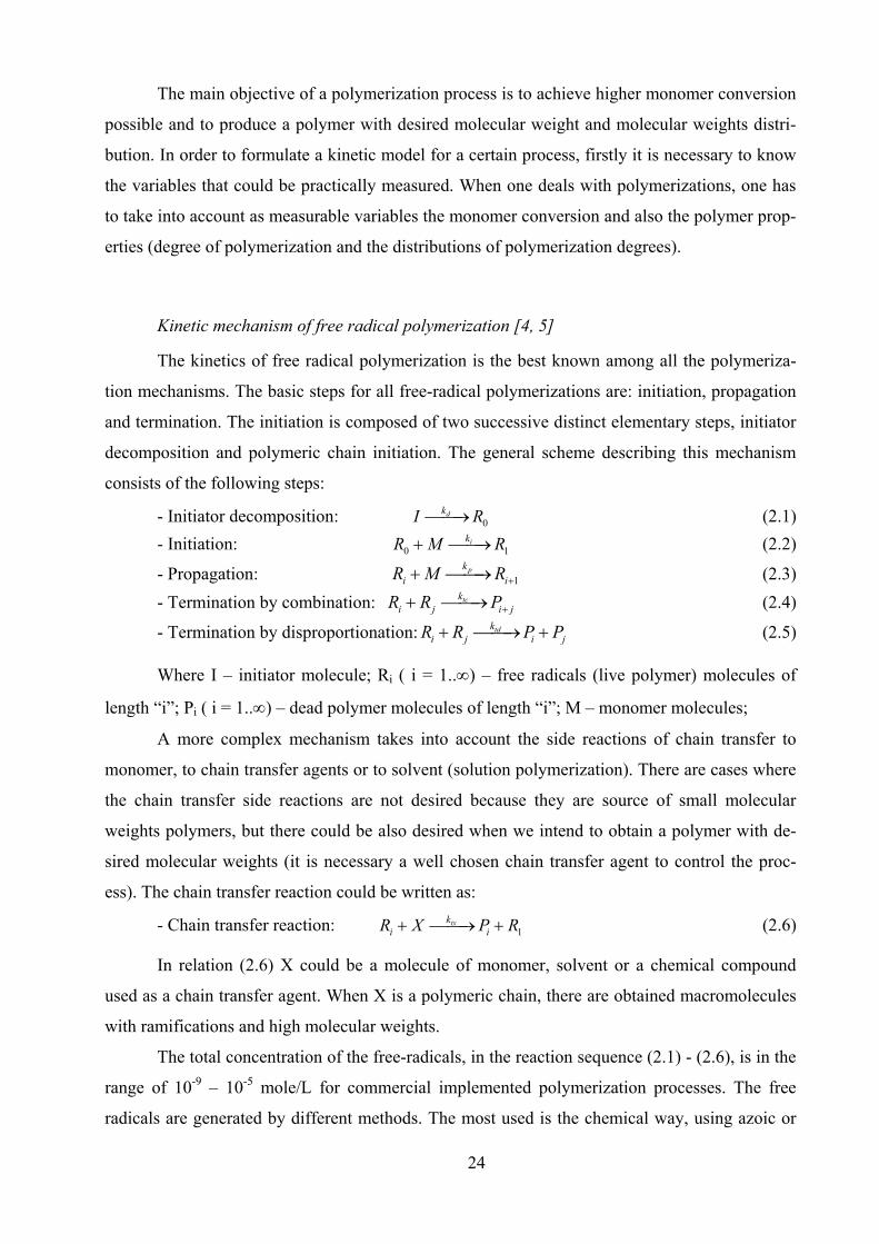
tion mechanisms. The basic steps for all free-radical polymerizations are: initiation, propagation
and termination. The initiation is composed of two successive distinct elementary steps, initiator
decomposition and polymeric chain initiation. The general scheme describing this mechanism
consists of the following steps:
- Initiator decomposition: 0dk
I R⎯⎯→ (2.1)
- Initiation: 0 1ik
R M R+ ⎯⎯→ (2.2)
- Propagation: 1pk
i iR M R ++ ⎯⎯→ (2.3)
- Termination by combination: tck
i j i jR R P++ ⎯⎯→ (2.4)
- Termination by disproportionation: tdk
i j i jR R P P+ ⎯⎯→ + (2.5)
Where I – initiator molecule; Ri ( i = 1..∞) – free radicals (live polymer) molecules of
length “i”; Pi ( i = 1..∞) – dead polymer molecules of length “i”; M – monomer molecules;
A more complex mechanism takes into account the side reactions of chain transfer to
monomer, to chain transfer agents or to solvent (solution polymerization). There are cases where
the chain transfer side reactions are not desired because they are source of small molecular
weights polymers, but there could be also desired when we intend to obtain a polymer with de-
sired molecular weights (it is necessary a well chosen chain transfer agent to control the proc-
ess). The chain transfer reaction could be written as:
- Chain transfer reaction: 1txk
i iR X P R+ ⎯⎯→ + (2.6)
In relation (2.6) X could be a molecule of monomer, solvent or a chemical compound
used as a chain transfer agent. When X is a polymeric chain, there are obtained macromolecules
with ramifications and high molecular weights.
The total concentration of the free-radicals, in the reaction sequence (2.1) - (2.6), is in the
range of 10-9 – 10-5 mole/L for commercial implemented polymerization processes. The free
radicals are generated by different methods. The most used is the chemical way, using azoic or
25
peroxide compounds in small concentrations (< 1 % wt). For example, the organic peroxides are
thermally decomposed by cleavage of the O – O chemical liaison. The efficiency of the initiator
is usually in the range 0.2 – 1 [6]. The principal cause of losing initiator efficiency is the so
called cage effect. At the initiator decomposition, the primary radicals are one in the vicinity of
the others a time of 10-10 – 10-9 s. In this interval, the radicals are walled by solvent molecules
among which they have to diffuse to initiate the polymerization reaction. The other ways to initi-
ate a polymerization reaction are thermally, UV radiations, high energy electron beam or gamma
radiations.
The propagation reaction (2.3) controls the rate of growth of the polymeric chain and its
structure. In free radical polymerization the microstructure of the polymeric chain is not influ-
enced by the initiation reaction mechanism and the initiator type. The termination reactions
(combination and disproportionation) take place simultaneously and their importance depends on
the monomer type and polymerization temperature. In the styrene polymerization, for instance,
the termination by combination is predominant on a certain temperature range. For the methyl
methacrylate polymerization, both terminations are important at small temperature, whereas at
high temperatures the termination by disproportionation is predominant.
At high monomer conversions, when the circulation of the radicals is hindered due to the
high reaction mixture viscosity, the active centers can continue to move and to produce bimol-
ecular termination reactions. So, the termination rate is independent of the length of the poly-
meric chain. Recently it was demonstrated that the bimolecular termination can be diffusion con-
trolled also at small monomer conversions [4].
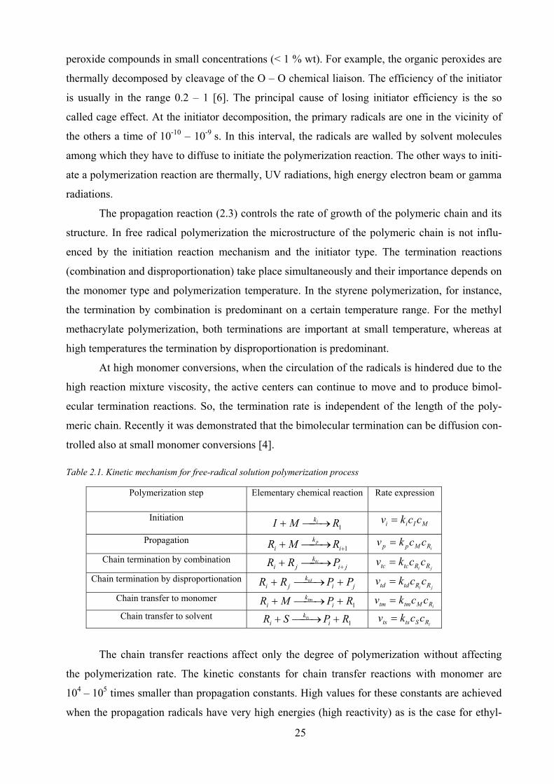
Table 2.1. Kinetic mechanism for free-radical solution polymerization process
Polymerization step Elementary chemical reaction Rate expression
Initiation 1RMI ik⎯→⎯+
MIii cckv =
Propagation 1+⎯→⎯+ i
k
i RMR p
iRMpp cckv =
Chain termination by combination ji
k
ji PRR tc +⎯→⎯+ ji RRtctc cckv =
Chain termination by disproportionation
ji
k
ji PPRR td +⎯→⎯+ ji RRtdtd cckv =
Chain transfer to monomer
1RPMR i
k
itm +⎯→⎯+
iRMtmtm cckv =
Chain transfer to solvent 1RPSR i
k
its +⎯→⎯+
iRStsts cckv =
The chain transfer reactions affect only the degree of polymerization without affecting
the polymerization rate. The kinetic constants for chain transfer reactions with monomer are
104 – 105 times smaller than propagation constants. High values for these constants are achieved
when the propagation radicals have very high energies (high reactivity) as is the case for ethyl-

26
ene, vinyl acetate and vinyl chloride polymerizations.
Based on the elementary steps (2.1) - (2.6), and considering only monomer and solvent as
involved chain transfer species, the rate expressions for a free-radical solution polymerization are
presented in Table 2.1. The overall chain termination constant is defined as the summation of the
termination by combination and disproportionation rate constants, t tc tdk k k= + .
Hypotheses used for the kinetic modeling of polymerization reactions
Regarding the reactants depletion, the limitative reactant could be the monomer (as in
majority of the cases) or the initiator (so called “dead – end”). A complex polymerization reac-
tion concerns elementary steps and there are involved chemical species with high and low mo-
lecular weights. The reactivity of the macromolecules is given by the end groups or the active
intermediates (free-radicals, ions, catalytic complexes). In the most cases it is applied the princi-
ple of equal reactivity which is stating that the reactivity of a polymeric chain is given only by its
end groups and it is independent of the chain length. In that case we can use a single kinetic con-
stant for all the propagation elementary steps. The other simplifications that could be used are
the QSSA (quasi steady state assumption) and long chains approximation. The long chains ap-
proximation is base on the hypothesis that the monomer is consumed predominantly to produce
polymers in the propagation step. The validity of this approximation could be confirmed study-
ing the degree of polymerization, that in the case of the invalidation is relatively small [6].
Most of the polymerization reactions sequence involve active intermediary (free-radicals,
ionic radicals, catalyst radicals). A characteristic of the chain reactions is a small concentration
of active species all long the process (a typical value for the free-radical polymerization is 10-8
mole/L) [6]. A problem that is raised is the validity of the QSSA in situations of practical interest
(high variations in kinetic constants, high rates of initiator consumption, hindered termination
reactions, non-uniformities in temperature profiles).
It is also accepted that the rates expressions valid for QSSA applied to close systems are
also valid for continuous reactors. It is proven that QSSA can be applied without significant er-
rors when the life time of the active species is much shorter than the residence time of the reac-
tion mixture in the reactor (i.e. free-radical polymerization).
Another approximation frequently used in the polymerization modeling is the constant
density and viscosity of the reaction mixture [5-8]. This represents simplified approaches and,
when more accurate results are desired, it is necessary to develop realistic viscosity models for
the studied polymerization processes.
27
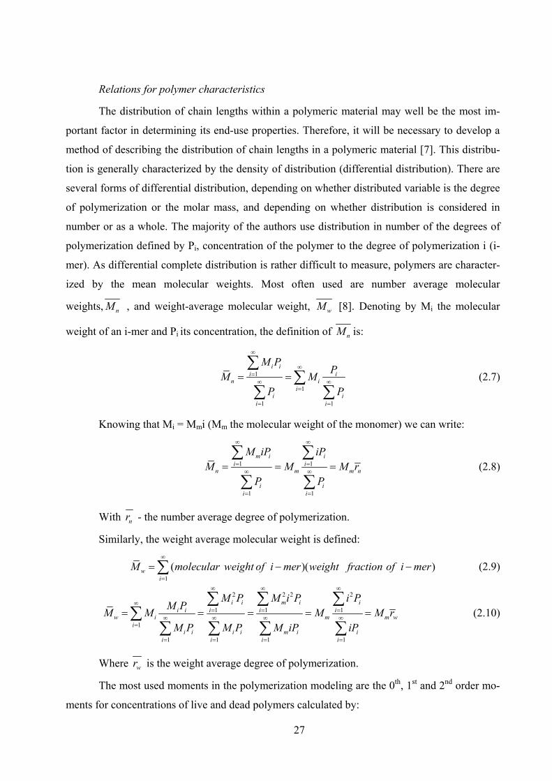
Relations for polymer characteristics
The distribution of chain lengths within a polymeric material may well be the most im-
portant factor in determining its end-use properties. Therefore, it will be necessary to develop a
method of describing the distribution of chain lengths in a polymeric material [7]. This distribu-
tion is generally characterized by the density of distribution (differential distribution). There are
several forms of differential distribution, depending on whether distributed variable is the degree
of polymerization or the molar mass, and depending on whether distribution is considered in
number or as a whole. The majority of the authors use distribution in number of the degrees of
polymerization defined by Pi, concentration of the polymer to the degree of polymerization i (i-
mer). As differential complete distribution is rather difficult to measure, polymers are character-
ized by the mean molecular weights. Most often used are number average molecular
weights, nM , and weight-average molecular weight, wM [8]. Denoting by Mi the molecular
weight of an i-mer and Pi its concentration, the definition of nM is:
1
1
1 1
i i
i in i
ii i
i i
M PP
M M
P P
∞∞= ∞ ∞=
= =
= =∑ ∑∑ ∑ (2.7)
Knowing that Mi = Mmi (Mm the molecular weight of the monomer) we can write:
1 1
1 1
m i i
i in m m n
i i
i i
M iP iP
M M M r
P P
∞ ∞
= =∞ ∞
= =
= = =∑ ∑∑ ∑ (2.8)
With nr - the number average degree of polymerization.
Similarly, the weight average molecular weight is defined:
1
( )( )w
i
M molecular weight of i mer weight fraction of i mer∞
== − −∑ (2.9)
2 2 2 2
1 1 1
1
1 1 1 1
i i m i i
i i i i iw i m m w
ii i i i m i i
i i i i
M P M i P i PM P
M M M M r
M P M P M iP iP
∞ ∞ ∞∞ = = =∞ ∞ ∞ ∞=
= = = =
= = = = =∑ ∑ ∑∑ ∑ ∑ ∑ ∑ (2.10)
Where wr is the weight average degree of polymerization.
The most used moments in the polymerization modeling are the 0th, 1st and 2nd order mo-
ments for concentrations of live and dead polymers calculated by:

28
20 1 2
1 1 1
20 1 2
1 1 1
; ;
; ;
i i i
i i i
i i i
i i i
P iP i P
R iR i R
μ μ μλ λ λ
∞ ∞ ∞
= = =∞ ∞ ∞
= = =
= = == = =
∑ ∑ ∑∑ ∑ ∑ (2.11)
If we consider that in the reaction mixture we have a dead and live polymers, the number
and weight average degree of polymerization could be also defined:
1 1 2 2
0 0 1 1
;n wr rμ λ μ λμ λ μ λ
+ += =+ + (2.12)
The structural homogeneity of the polymer mixture is usually characterized by the poly-
dispersion index, defined as the ratio of the two degrees of polymerization:
w
n
rIP
r= (2.13)
2.1.4. Methyl methacrylate polymerization
The acrylic acid and acrylate esters are known since the middle of the 19th century. A re-
view of acrylate esters was published in 1901 by H. Von Pechmann and O. Rohm [4, 9]. An
industrial production process of acrylates was developed in 1928 by W. Bauer [10]. Solution
polymers were produced from methyl methacrylate since 1927 by Rohm and Haas (Germany).
Emulsion polymers were first developed on an industrial scale in 1929 - 1930 by H. Fikentscher,
and were introduced on the market by BASF as a polymer dispersion named "Corialgrund" for
the surface finishing of leather [4].
Acrylates can be polymerized extremely easily because their carboxyl groups are adjacent
to a vinyl group. Polyacrylates are produced almost exclusively by radical polymerization; con-
ventional radical formers (e.g., peroxides and other per compounds) or azo starters are used as
initiators. Polymerization can also be initiated photochemically, by け-rays, or by electron beams.
Although ionic (particularly anionic) polymerization is possible, this process is not used industri-
ally. The heat of reaction in the exothermic polymerization of acrylates is cca. 60 – 80 kJ/mol,
and must be removed if the process is to be controlled effectively [4].
Several general disadvantages of bulk polymerization (removal of the reaction heat, in-
solubility of the resulting polymer in the monomer, side reactions in highly viscous systems such
as the Trommsdorff effect or chain transfer with polymer) are responsible for the fact that many
polymerization processes are carried out in the presence of a solvent [9].
Acrylates are polymerized as solutions in organic solvents [12-18] if the user wishes to
exploit specific properties of polymers in dissolved form (e.g., low molecular mass, good flow
29
behavior, and homogeneous film formation after drying in paints or adhesives). Aromatic hydro-
carbons such as benzene and toluene [12-18] can be used as solvents for the polymerization of
acrylates of long-chain alcohols; esters (i. e. ethyl acetate [11, 12]) and ketones can be used for
acrylates of short-chain alcohols [4].
Gel effect models for MMA free radical polymerization
At low monomer conversions, the viscosity of the reaction mixture is low, and the rate of
reaction is controlled by the segmental diffusion (internal reorientation of the polymer chains
required to bring the chains together for the polymerization take place) [3, 13]. In this stage of
the process, the termination rate have relatively high values (order of magnitude 108 L mol-1 s-1
or higher). However, the viscosity of the reaction mixture increases rapidly with the monomer
conversion (polymer concentration) and the rate at which two polymer chains encounter each
other is slower than in the segmental reorientation. Consequently, the polymerization kinetics is
controlled by the low frequency of reciprocal collisions of live chains through the mixtures of
dead polymers. As known, the translational diffusion is affected both by chain length of the re-
acting polymers and the system viscosity [3].
At high monomer conversions, the system becomes so viscous that the polymers size in-
creases more quickly due to propagation than by reciprocal combinations (due to the resistance
opposed by reaction mixture to polymer diffusion). The diffusional limitations of the live and
polymer dynamics, with strong effects on the propagation as well as termination rates (lowering
its values) are called gel effect (or Trommsdorff effect).
Modeling the gel effect presents significant difficulties, due to the particularities of the
phenomenon. As specified, its influence becomes important at high monomer conversions, par-
ticularly for bulk polymerization. However it can be significant also for solution polymerization,
at high monomer to solvent ratios.
Free radical solution polymerization of MMA follows the mechanism presented in the
previous paragraph. The considerable increase in the polymerization rate and in the average
chain length at intermediate conversions is a phenomenon common to many monomers undergo-
ing free radical polymerization [14]. The termination rate depends on the polymerization tem-
perature, the mobility of the polymeric chains (diffusion), the molecular weights of the involved
species and the composition of the reaction mixture.
During the last decades, several studies have been devoted to develop an isothermal dif-
fusion-controlled model for the free radical polymerization of methyl-methacrylate (MMA).
The existing models can be separated into three groups: mechanistic, semi-empirical, and
30
fully empirical. Mechanistic models, developed during the middle to late seventies period, fo-
cused mainly on reptation theory (developed to explain the dynamics of entangled molecules in a
network of fixed obstacles) and scaling concepts [15] while the semi-empirical models made use
of many different variations on free volume theory [13].
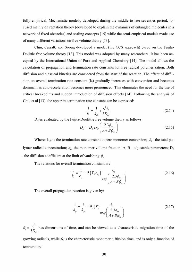
Chiu, Carratt, and Soong developed a model (the CCS approach) based on the Fujita-
Dolittle free volume theory [13]. This model was adopted by many researchers. It has been ac-
cepted by the International Union of Pure and Applied Chemistry [14]. The model allows the
calculation of propagation and termination rate constants for free radical polymerization. Both
diffusion and classical kinetics are considered from the start of the reaction. The effect of diffu-
sion on overall termination rate constant (kt) gradually increases with conversion and becomes
dominant as auto-acceleration becomes more pronounced. This eliminates the need for the use of
critical breakpoints and sudden introduction of diffusion effects [14]. Following the analysis of
Chiu et al [13], the apparent termination rate constant can be expressed:
2
0
0
1 1
3t
t t ef
r
k k D
λ= + (2.14)
Def is evaluated by the Fujita-Doolittle free volume theory as follows:
0
2.3exp m
ef
m
D DA B
φφ
⎛ ⎞= ⎜ ⎟+⎝ ⎠ (2.15)
Where: kt,0 is the termination rate constant at zero monomer conversion; 0λ - the total po-
lymer radical concentration; mφ -the monomer volume fraction; A, B - adjustable parameters; D0
-the diffusion coefficient at the limit of vanishing mφ .
The relations for overall termination constant are:
( )0
0
01 1,
2.3exp
t I
t t m
m
T ck k
A B
λθ φφ
= + ⎛ ⎞⎜ ⎟+⎝ ⎠ (2.16)
The overall propagation reaction is given by:
( )0
01 1
2.3exp
p
p p m
m
Tk k
A B
λθ φφ
= + ⎛ ⎞⎜ ⎟+⎝ ⎠ (2.17)
3
3t
t
ef
r
Dθ = has dimensions of time, and can be viewed as a characteristic migration time of the
growing radicals, while tθ is the characteristic monomer diffusion time, and is only a function of
temperature.

31
The global rate constants for termination and propagation defined by these equations are
calculated as the contributions of a purely chemical kinetic constant (the first term on the right
hand side of both equations) and a purely diffusional one respectively (the second term on the
right hand side of both equations). A and B are also treated as adjustable parameters and can be
derived from experimental data. In addition, in the cited study of Chiu [20], tθ was found by
fitting experimental data which only considered AIBN as the initiator.
With other initiators, the kinetics will affect how the chain length varies with initiator
loading. Therefore the correlation is not valid for other polymer/initiator systems [14].
Expressions for overall termination and propagation reactions were derived by Baillagou
and Soong [16, 17] based on the kinetic data of Chiu et al [13]. The expressions (2.16) - (2.17)
are rewritten as:
0 0
0 00 0
;
1 1
t p
t pt t p p
ef ef
k kk k
k k
D D
θ λ θ λ= =+ +
(2.18)
Chiu et al [13] proposed a constant value of 0.03 for parameter B (expression (2.17)), be-
cause it was found to be relatively insensitive to the working conditions.
Also, the parameter A was determined from experimental data and is given by the expres-
sion:
( )260.168 8.21 10 gpA T T−= − ⋅ − , (2.19)
where Tg =114 °C is the glass transition temperature for the polymer.
The gel-effect model of Chiu, Carrat and Soong are presented in a condensed mode in
Table 2.2. The gel-effect model published by Fleury and reviewed by Nising [18] is an approach
based on the model published by Chiu, Carrat and Soong. The aim of Fleury was to linearize the
expression (2.16) of the apparent termination rate constant. The model is a good example of a
semi-empirical approach adapted to the experimental conditions. The equation (2.16) was modi-
fied as:
( )0
1 1 1
expt tk k Xα β= + − × (2.20)
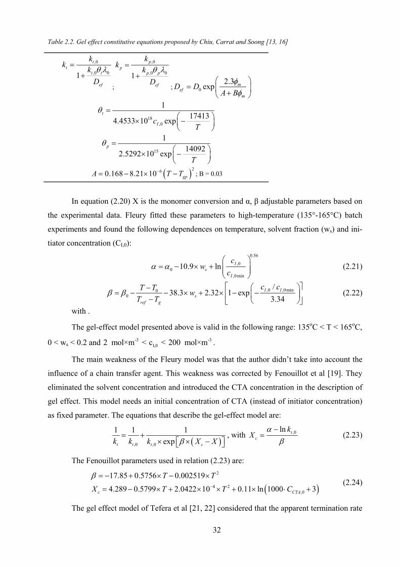
32
Table 2.2. Gel effect constitutive equations proposed by Chiu, Carrat and Soong [13, 16]
,0
,0 01
t
tt t
ef
kk
k
D
θ λ=+
;
,0
,0 01
p
pp p
ef
kk
k
D
θ λ=+
; 0
2.3exp m
ef
m
D DA B
φφ
⎛ ⎞= ⎜ ⎟+⎝ ⎠
18,0
117413
4.4533 10 expt
IcT
θ = ⎛ ⎞× −⎜ ⎟⎝ ⎠
15
114092
2.5292 10 exp= ⎛ ⎞× −⎜ ⎟⎝ ⎠
p
T
θ
( )260.168 8.21 10−= − × − gpA T T ; B = 0.03
In equation (2.20) X is the monomer conversion and α, く adjustable parameters based on
the experimental data. Fleury fitted these parameters to high-temperature (135°-165°C) batch
experiments and found the following dependences on temperature, solvent fraction (ws) and ini-
tiator concentration (CI,0):
0.56
,00
,0min
10.9 ln I
s
I
cw
cα α ⎛ ⎞= − × + ⎜ ⎟⎜ ⎟⎝ ⎠ (2.21)
,0 ,0min00
/38.3 2.32 1 exp
3.34I I
s
ref g
c cT Tw
T Tβ β ⎡ ⎤⎛ ⎞−= − − × + × − −⎢ ⎥⎜ ⎟− ⎝ ⎠⎣ ⎦ (2.22)
with .
The gel-effect model presented above is valid in the following range: 135oC < T < 165oC,
0 < ws < 0.2 and -3 -3I,02 mol×m < c < 200 mol×m .
The main weakness of the Fleury model was that the author didn’t take into account the
influence of a chain transfer agent. This weakness was corrected by Fenouillot et al [19]. They
eliminated the solvent concentration and introduced the CTA concentration in the description of
gel effect. This model needs an initial concentration of CTA (instead of initiator concentration)
as fixed parameter. The equations that describe the gel-effect model are:
( ),0 ,0
1 1 1
expt t t ck k k X Xβ= + × × −⎡ ⎤⎣ ⎦ , with ,0ln t
c
kX
αβ
−= (2.23)
The Fenouillot parameters used in relation (2.23) are:
( )2
4 2,0
17.85 0.5756 0.002519
4.289 0.5799 2.0422 10 0.11 ln 1000 3c CTA
T T
X T T C
β−
= − + × − ×= − × + × × + × ⋅ + (2.24)
The gel effect model of Tefera et al [21, 22] considered that the apparent termination rate
33
constant is governed by three mechanisms: the segmental diffusion, at the early polymerization
stages, the translational diffusion at intermediate conversions and the reaction diffusion taking
place through the whole reaction. The model is based on the free volume theory and one of its
advantages is inclusion of the molecular weight dependence. The model was reported to work in
polymerization systems with CTA agents.
Published kinetic models for MMA polymerization in solution
The kinetics of the MMA polymerization process in solution was investigated in an im-
portant number of experimental and theoretical studies, proposing their own kinetic models. The
temperature dependences of reaction rate constants involved in the rate expressions presented in
Table 2.1 were also investigated in a significant number of published works.
The expressions for the rate constants proposed by different authors are presented in
Table 2.4 and the working conditions corresponding to these kinetic studies are presented in
Table 2.3.
2.1.5. Mathematical models for tubular MMA polymerization reactor
Plug flow reactor model
The plug flow reactor becomes a viable alternative in polymer processing when it is de-
sired to exploit the kinetic advantages of the batch reactors (high conversions) and the opera-
tional advantages of continuous processing (easy operation, lack of batch-to-batch variability).
Tubular reactors (approximating plug flow characteristics) are applicable in high-volume polym-
erizations and exhibit excellent heat transfer capabilities [7].
The mass balance equation for a species X in a plug-flow polymerization reactor could be
written as:
( )z x
x
d u cr
dz= (2.25)
Where uz is the velocity of the reactor mixture. In expression (2.25) the index x can de-
note initiator (I), monomer (M), radical concentrations distribution moments ( , 0..2i iλ = ) or
polymers concentrations distribution moments ( , 0..2i iμ = ).
The consumption rates, rx, for MMA solution polymerization can be determined based on
the kinetic scheme in Table 2.1. In this case the density variation of the reaction mixture was
taken into account. Such a model was implemented by Ahn et al [20], Chang et al [21, 22].
When no density variations are taken into account, the equations (2.25) are simplified to:
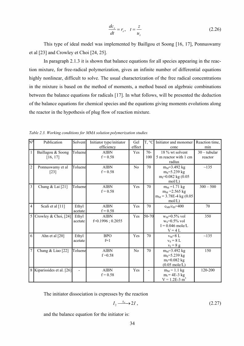
34
,xx
z
dc zr t
dt u= = (2.26)
This type of ideal model was implemented by Baillgou et Soong [16, 17], Ponnuswamy
et al [23] and Crowley et Choi [24, 25].
In paragraph 2.1.3 it is shown that balance equations for all species appearing in the reac-
tion mixture, for free-radical polymerization, gives an infinite number of differential equations
highly nonlinear, difficult to solve. The usual characterization of the free radical concentrations
in the mixture is based on the method of moments, a method based on algebraic combinations
between the balance equations for radicals [17]. In what follows, will be presented the deduction
of the balance equations for chemical species and the equations giving moments evolutions along
the reactor in the hypothesis of plug flow of reaction mixture.
Table 2.3. Working conditions for MMA solution polymerization studies
No Publication Solvent Initiator type/initiator efficiency
Gel effect
T, °C Initiator and monomer conc
Reaction time, min
1 Baillagou & Soong [16, 17]
Toluene AIBN f = 0.58
Yes 70-100
18 % wt solvent 5 m reactor with 1 cm
radius
30 – tubular reactor
2 Ponnuswamy et al [23]
Toluene AIBN f = 0.58
No 70 mM=3.492 kg mS=5.239 kg
mI=0.082 kg (0.05 mol/L)
~135
3 Chang & Lai [21] Toluene AIBN f = 0.58
Yes 70 mM =1.71 kg mM =2.565 kg
mM = 3.78E-4 kg (0.05 mol/L)
300 – 500
4 Scali et al [11] Ethyl acetate
AIBN f = 0.58
Yes 70 cM0/cI0=400 70
5 Crowley & Choi, [24] Ethyl acetate
AIBN f=0.1996 ; 0.2055
Yes 50-70 wM=0.5% vol wS=0.5% vol
I = 0.046 mole/L V = 4 L
350
6 Ahn et al [20] Ethyl acetate
BPO f=1
Yes 70 vM=8 L vS = 8 L vI = 8 g
~135
7 Chang & Liao [22] Toluene AIBN f =0.58
No 70 mM=3.492 kg mS=5.239 kg mI=0.082 kg (0.05 mole/L)
150
8 Kiparissides et al. [26] - AIBN f = 0.58
Yes - mM = 1.1 kg mI = 4E-3 kg
V = 1.2E-3 m3
120-200
The initiator dissociation is expresses by the reaction
2 2dkI I⎯⎯→ , (2.27)
and the balance equation for the initiator is:
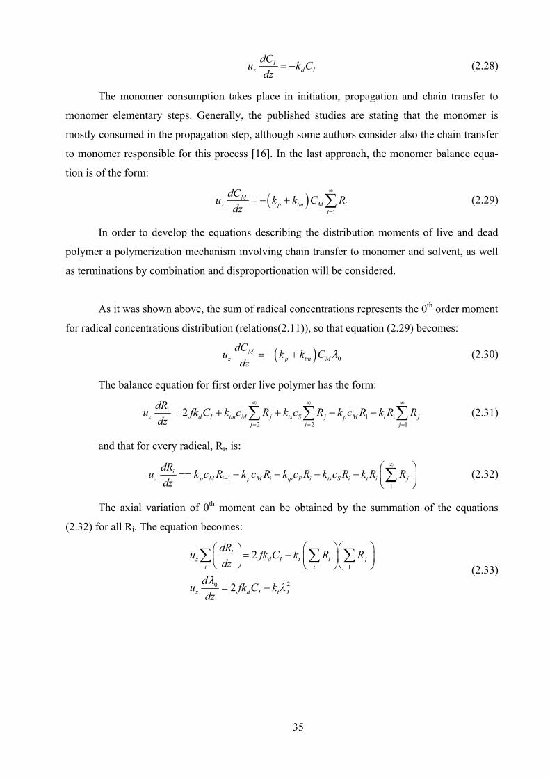
35
Iz d I
dCu k C
dz= − (2.28)
The monomer consumption takes place in initiation, propagation and chain transfer to
monomer elementary steps. Generally, the published studies are stating that the monomer is
mostly consumed in the propagation step, although some authors consider also the chain transfer
to monomer responsible for this process [16]. In the last approach, the monomer balance equa-
tion is of the form:
( )1
Mz p tm M i
i
dCu k k C R
dz
∞
== − + ∑ (2.29)
In order to develop the equations describing the distribution moments of live and dead
polymer a polymerization mechanism involving chain transfer to monomer and solvent, as well
as terminations by combination and disproportionation will be considered.
As it was shown above, the sum of radical concentrations represents the 0th order moment
for radical concentrations distribution (relations(2.11)), so that equation (2.29) becomes:
( ) 0M
z p tm M
dCu k k C
dzλ= − + (2.30)
The balance equation for first order live polymer has the form:
11 1
2 2 1
2z d I tm M j ts S j p M t j
j j j
dRu fk C k c R k c R k c R k R R
dz
∞ ∞ ∞
= = == + + − −∑ ∑ ∑ (2.31)
and that for every radical, Ri, is:
11
iz p M i p M i tp P i ts S i t i j
dRu k c R k c R k c R k c R k R R
dz
∞−
⎛ ⎞== − − − − ⎜ ⎟⎝ ⎠∑ (2.32)
The axial variation of 0th moment can be obtained by the summation of the equations
(2.32) for all Ri. The equation becomes:
1
200
2
2
iz d I t i j
i i
z d I t
dRu fk C k R R
dz
du fk C k
dz
λ λ
⎛ ⎞⎛ ⎞⎛ ⎞ = −⎜ ⎟ ⎜ ⎟⎜ ⎟⎝ ⎠ ⎝ ⎠⎝ ⎠= −
∑ ∑ ∑ (2.33)
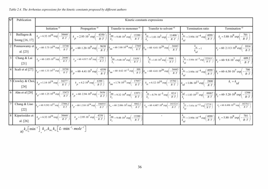
36
Table 2.4. The Arrhenius expressions for the kinetic constants proposed by different authors
a)1mindk −⎡ ⎤⎣ ⎦ ,
1 1,, minp tm tsk k k L mole− −⎡ ⎤⋅ ⋅⎣ ⎦
Kinetic constants expressions No Publication
Initiation a) Propagation a) Transfer to monomer a) Transfer to solvent a) Termination ratio Termination a)
1 Baillagou &
Soong [16, 17]
30660166.32 10 expkd R T
⎛ ⎞= ⋅ −⎜ ⎟⋅⎝ ⎠
435072.95 10 expkp R T
⎛ ⎞= ⋅ −⎜ ⎟⋅⎝ ⎠
1338039.48 10 expp
ktm
k R T
⎛ ⎞= ⋅ −⎜ ⎟⋅⎝ ⎠1140031.01 10 exp
p
kts
k R T
⎛ ⎞= ⋅ −⎜ ⎟⋅⎝ ⎠
409043.956 10 expktc
k R Ttd
⎛ ⎞−= ⋅ ⎜ ⎟⋅⎝ ⎠70195.88 10 expk
t R T
⎛ ⎞= ⋅ −⎜ ⎟⋅⎝ ⎠
2 Ponnuswamy et
al. [23]
337401660 3.75 10 expkd R T
⎛ ⎞= ⋅ ⋅ −⎜ ⎟⋅⎝ ⎠ 9630960 1.20 10 expk
p R T
⎛ ⎞= ⋅ ⋅ −⎜ ⎟⋅⎝ ⎠276031460 3.88 10 expk
tm R T
⎛ ⎞= ⋅ ⋅ −⎜ ⎟⋅⎝ ⎠344432060 4.41 10 expk
ts R T
⎛ ⎞= ⋅ ⋅ −⎜ ⎟⋅⎝ ⎠ 1ktc
ktd
=
1014860 2.113 10 expkt R T
⎛ ⎞= ⋅ ⋅ −⎜ ⎟⋅⎝ ⎠
3 Chang & Lai
[21]
266401560 1.053 10 expkd R T
⎛ ⎞= ⋅ ⋅ −⎜ ⎟⋅⎝ ⎠ 3781560 4.917 10 expk
p R T
⎛ ⎞= ⋅ ⋅ −⎜ ⎟⋅⎝ ⎠ 1163039.48 10 exp
p
ktm
k R T
⎛ ⎞= ⋅ −⎜ ⎟⋅⎝ ⎠
9908 31.01 10 expp
kts
k R T
⎛ ⎞= ⋅ −⎜ ⎟⋅⎝ ⎠
3554.833.956 10 expktc
k R Ttd
⎛ ⎞−= ⋅ ⎜ ⎟⋅⎝ ⎠
609.2760 9.8 10 expkt R T
⎛ ⎞= ⋅ ⋅ −⎜ ⎟⋅⎝ ⎠
4 Scali et al [27] 307001560 1.33 10 expkd R T
⎛ ⎞= ⋅ ⋅ −⎜ ⎟⋅⎝ ⎠ 4350560 4.41 10 expk
p R T
⎛ ⎞= ⋅ ⋅ −⎜ ⎟⋅⎝ ⎠888260 4.62 10 expk
tm R T
⎛ ⎞−= ⋅ ⋅ −⎜ ⎟⋅⎝ ⎠344432060 4.41 10 expk
ts R T
⎛ ⎞= ⋅ ⋅ −⎜ ⎟⋅⎝ ⎠ 409043.956 10 expktc
k R Ttd
⎛ ⎞−= ⋅ ⎜ ⎟⋅⎝ ⎠700760 6.50 10 expk
t R T
⎛ ⎞= ⋅ ⋅ −⎜ ⎟⋅⎝ ⎠
5 Crowley & Choi,
[24]
34277191.14 10 expkd R T
⎛ ⎞= ⋅ −⎜ ⎟⋅⎝ ⎠
630084.2 10 expkp R T
⎛ ⎞= ⋅ −⎜ ⎟⋅⎝ ⎠
17957131.74 10 expktm R T
⎛ ⎞= ⋅ −⎜ ⎟⋅⎝ ⎠15702106.12 10 expk
ts R T
⎛ ⎞= ⋅ −⎜ ⎟⋅⎝ ⎠
2800111.06 10 expktd R T
⎛ ⎞= ⋅ −⎜ ⎟⋅⎝ ⎠ tk ktd
=
6 Ahn et al [20] 354731860 1.25 10 expkd R T
⎛ ⎞= ⋅ ⋅ −⎜ ⎟⋅⎝ ⎠
5656660 2.94 10 expkp R T
⎛ ⎞= ⋅ ⋅ −⎜ ⎟⋅⎝ ⎠1397149.32 10 exp
p
ktm
k R T
⎛ ⎞= ⋅ −⎜ ⎟⋅⎝ ⎠42.658.79 10 exp
p
kts
k R T
⎛ ⎞−= ⋅ −⎜ ⎟⋅⎝ ⎠
44467271.83 10 expktd
k R Tt
⎛ ⎞= ⋅ −⎜ ⎟⋅⎝ ⎠1394860 5.20 10 expk
t R T
⎛ ⎞= ⋅ ⋅ −⎜ ⎟⋅⎝ ⎠
7 Chang & Liao
[22]
27886.21560 9.592 10 expkd R T
⎛ ⎞= ⋅ ⋅ −⎜ ⎟⋅⎝ ⎠ 14669.81460 1.310 10 expk
p R T
⎛ ⎞= ⋅ ⋅ −⎜ ⎟⋅⎝ ⎠8862.1160 2.886 10 exptmk
R T
⎛ ⎞= ⋅ ⋅ −⎜ ⎟⋅⎝ ⎠14152.8660 4.487 10 expk
ts R T
⎛ ⎞= ⋅ ⋅ −⎜ ⎟⋅⎝ ⎠12718127.976 10 exp
ktc
k R Ttd
⎛ ⎞−= ⋅ ⎜ ⎟⋅⎝ ⎠
18378.32160 8.498 10 expkt R T
⎛ ⎞= ⋅ ⋅ −⎜ ⎟⋅⎝ ⎠
8 Kiparissides et
al. [26]
30660166.32 10 expkd R T
⎛ ⎞= ⋅ −⎜ ⎟⋅⎝ ⎠
435072.95 10 expkp R T
⎛ ⎞= ⋅ −⎜ ⎟⋅⎝ ⎠ 1338039.48 10 exp
p
ktm
k R T
⎛ ⎞= ⋅ −⎜ ⎟⋅⎝ ⎠- 409043.956 10 exp
ktc
k R Ttd
⎛ ⎞−= ⋅ ⎜ ⎟⋅⎝ ⎠70195.88 10 expk
t R T
⎛ ⎞= ⋅ −⎜ ⎟⋅⎝ ⎠
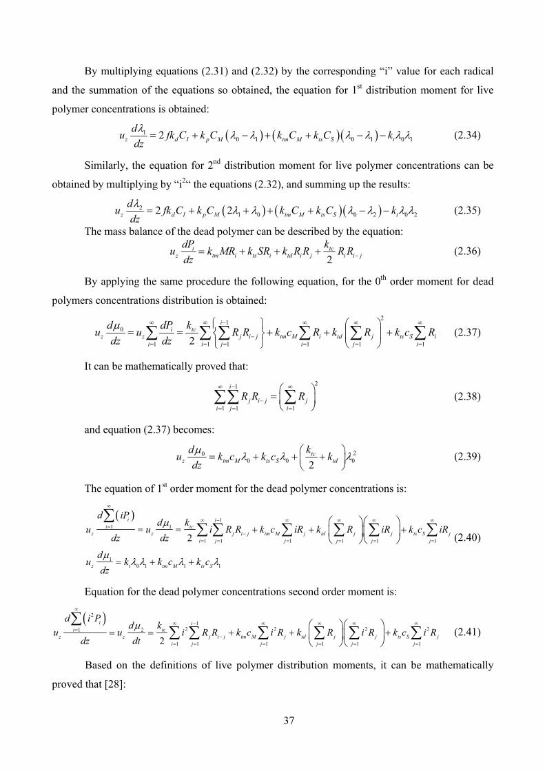
37
By multiplying equations (2.31) and (2.32) by the corresponding “i” value for each radical
and the summation of the equations so obtained, the equation for 1st distribution moment for live
polymer concentrations is obtained:
( ) ( )( )10 1 0 1 0 12z d I p M tm M ts S t
du fk C k C k C k C k
dz
λ λ λ λ λ λ λ= + − + + − − (2.34)
Similarly, the equation for 2nd distribution moment for live polymer concentrations can be
obtained by multiplying by “i2“ the equations (2.32), and summing up the results:
( ) ( )( )21 0 0 2 0 22 2z d I p M tm M ts S t
du fk C k C k C k C k
dz
λ λ λ λ λ λ λ= + + + + − − (2.35)
The mass balance of the dead polymer can be described by the equation:
2
i tcz tm i ts i td i j i i j
dP ku k MR k SR k R R R R
dz−= + + + (2.36)
By applying the same procedure the following equation, for the 0th order moment for dead
polymers concentrations distribution is obtained:
21
0
1 1 1 1 1 12
ii tc
z z j i j tm M i td j ts S i
i i j i j i
d dP ku u R R k c R k R k c R
dz dz
μ ∞ ∞ − ∞ ∞ ∞−= = = = = =
⎧ ⎫ ⎛ ⎞= = + + +⎨ ⎬ ⎜ ⎟⎩ ⎭ ⎝ ⎠∑ ∑ ∑ ∑ ∑ ∑ (2.37)
It can be mathematically proved that:
21
1 1 1
i
j i j j
i j i
R R R∞ − ∞
−= = =⎛ ⎞= ⎜ ⎟⎝ ⎠∑∑ ∑ (2.38)
and equation (2.37) becomes:
200 0 02
tcz tm M ts S td
d ku k c k c k
dz
μ λ λ λ⎛ ⎞= + + +⎜ ⎟⎝ ⎠ (2.39)
The equation of 1st order moment for the dead polymer concentrations is:
( ) 11 1
1 1 1 1 1 1
10 1 1 1
2
∞∞ − ∞ ∞ ∞ ∞=
−= = = = = =
= = + + +
= + +
⎛ ⎞⎛ ⎞⎜ ⎟⎜ ⎟⎝ ⎠⎝ ⎠∑ ∑ ∑ ∑ ∑ ∑ ∑i i
i tc
z z j i j tm M j td j j ts S j
i j j j j j
z t tm M ts S
d iPkd
u u i R R k c iR k R iR k c iRdz dz
du k k c k c
dz
μμ λ λ λ λ
(2.40)
Equation for the dead polymer concentrations second order moment is:
( )2
12 2 2 21 2
1 1 1 1 1 12
∞∞ − ∞ ∞ ∞ ∞=
−= = = = = =
= = + + +⎛ ⎞⎛ ⎞⎜ ⎟⎜ ⎟⎝ ⎠⎝ ⎠∑ ∑ ∑ ∑ ∑ ∑ ∑i i
i tc
z z j i j tm M j td j j ts S j
i j j j j j
d i Pkd
u u i R R k c i R k R i R k c i Rdz dt
μ (2.41)
Based on the definitions of live polymer distribution moments, it can be mathematically
proved that [28]:
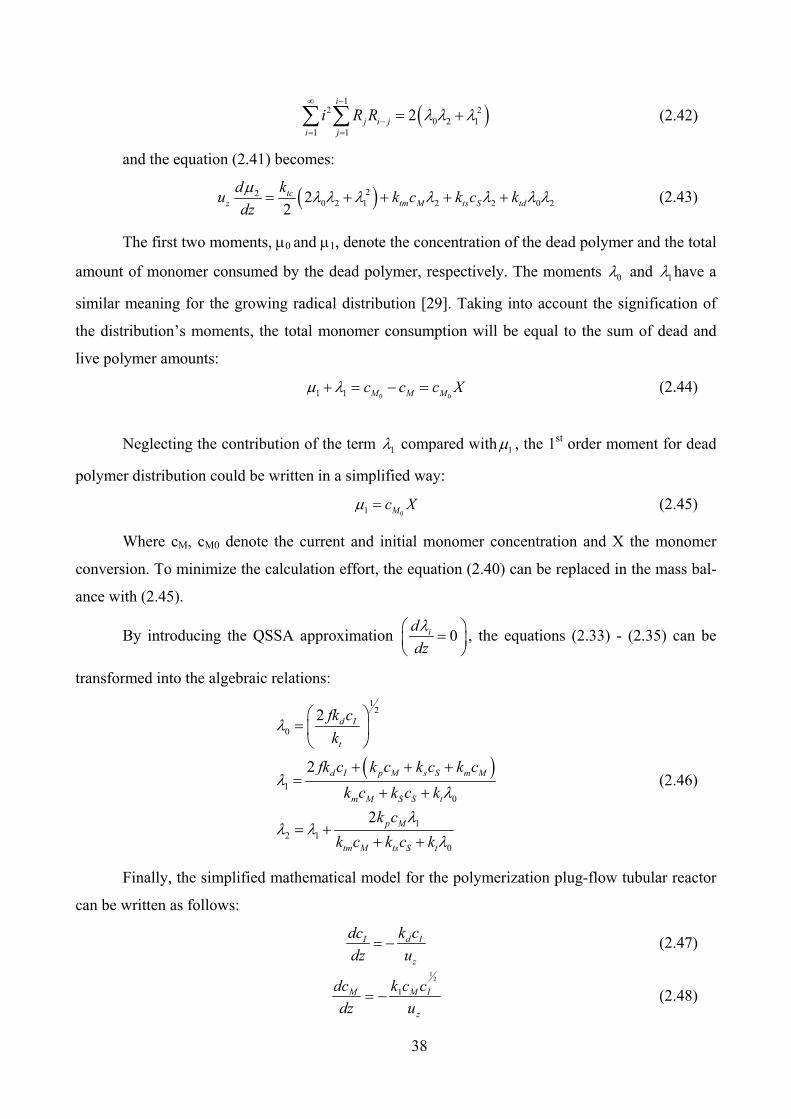
38
( )12 2
0 2 11 1
2i
j i j
i j
i R R λ λ λ∞ −−= =
= +∑ ∑ (2.42)
and the equation (2.41) becomes:
( )220 2 1 2 2 0 22
2tc
z tm M ts S td
kdu k c k c k
dz
μ λ λ λ λ λ λ λ= + + + + (2.43)
The first two moments, μ0 and μ1, denote the concentration of the dead polymer and the total
amount of monomer consumed by the dead polymer, respectively. The moments 0λ and 1λ have a
similar meaning for the growing radical distribution [29]. Taking into account the signification of
the distribution’s moments, the total monomer consumption will be equal to the sum of dead and
live polymer amounts:
0 01 1 M M Mc c c Xμ λ+ = − = (2.44)
Neglecting the contribution of the term 1λ compared with 1μ , the 1st order moment for dead
polymer distribution could be written in a simplified way:
01 Mc Xμ = (2.45)
Where cM, cM0 denote the current and initial monomer concentration and X the monomer
conversion. To minimize the calculation effort, the equation (2.40) can be replaced in the mass bal-
ance with (2.45).
By introducing the QSSA approximation 0id
dz
λ⎛ ⎞=⎜ ⎟⎝ ⎠ , the equations (2.33) - (2.35) can be
transformed into the algebraic relations:
( )
12
0
10
12 1
0
2
2
2
d I
t
d I p M s S m M
m M S S t
p M
tm M ts S t
fk c
k
fk c k c k c k c
k c k c k
k c
k c k c k
λ
λ λλλ λ λ
⎛ ⎞= ⎜ ⎟⎝ ⎠+ + += + +
= + + +
(2.46)
Finally, the simplified mathematical model for the polymerization plug-flow tubular reactor
can be written as follows:
d II
z
k cdc
dz u= − (2.47)
z
IMM
u
cck
dz
dc2
1
1−= (2.48)
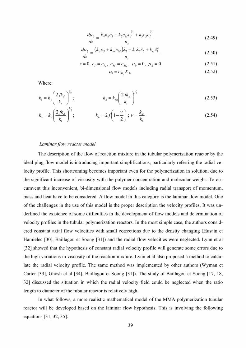
39
z
ISIMId
u
cckcckckk
dz
d2
12
1
3240 ++=μ (2.49)
( )
z
tctMtmSts
u
kkckck
dz
d212022 λλλλμ +++= (2.50)
0,0,,,0 2000===== μμMMII ccccz (2.51)
01 M Mc Xμ = (2.52)
Where:
21
1
2 ⎟⎟⎠⎞⎜⎜⎝
⎛=t
dp
k
fkkk ;
21
2
2 ⎟⎟⎠⎞⎜⎜⎝
⎛=t
dtm
k
fkkk (2.53)
21
3
2 ⎟⎟⎠⎞⎜⎜⎝
⎛=t
dts
k
fkkk ; ⎟⎠
⎞⎜⎝⎛ −=
2124
νfk ;
t
tc
k
k=ν (2.54)
Laminar flow reactor model
The description of the flow of reaction mixture in the tubular polymerization reactor by the
ideal plug flow model is introducing important simplifications, particularly referring the radial ve-
locity profile. This shortcoming becomes important even for the polymerization in solution, due to
the significant increase of viscosity with the polymer concentration and molecular weight. To cir-
cumvent this inconvenient, bi-dimensional flow models including radial transport of momentum,
mass and heat have to be considered. A flow model in this category is the laminar flow model. One
of the challenges in the use of this model is the proper description the velocity profiles. It was un-
derlined the existence of some difficulties in the development of flow models and determination of
velocity profiles in the tubular polymerization reactors. In the most simple case, the authors consid-
ered constant axial flow velocities with small corrections due to the density changing (Husain et
Hamielec [30], Baillagou et Soong [31]) and the radial flow velocities were neglected. Lynn et al
[32] showed that the hypothesis of constant radial velocity profile will generate some errors due to
the high variations in viscosity of the reaction mixture. Lynn et al also proposed a method to calcu-
late the radial velocity profile. The same method was implemented by other authors (Wyman et
Carter [33], Ghosh et al [34], Baillagou et Soong [31]). The study of Baillagou et Soong [17, 18,
32] discussed the situation in which the radial velocity field could be neglected when the ratio
length to diameter of the tubular reactor is relatively high.
In what follows, a more realistic mathematical model of the MMA polymerization tubular
reactor will be developed based on the laminar flow hypothesis. This is involving the following
equations [31, 32, 35]:
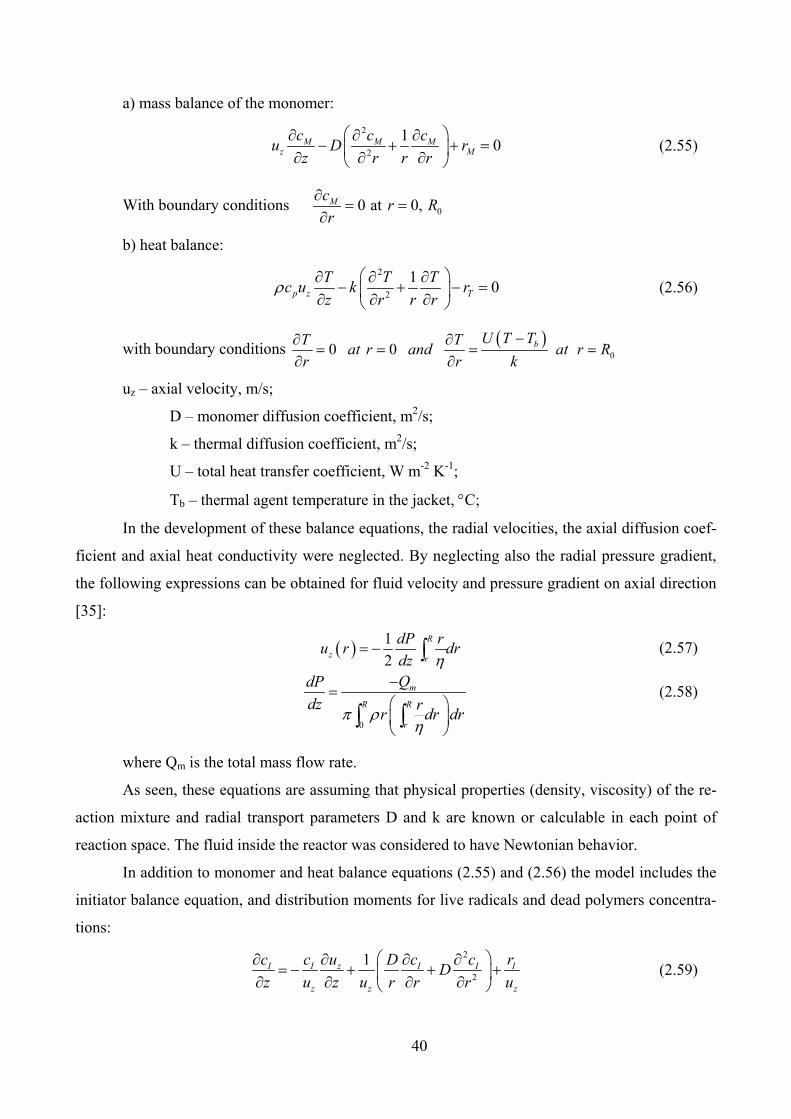
40
a) mass balance of the monomer:
2
2
10M M M
z M
c c cu D r
z r r r
⎛ ⎞∂ ∂ ∂− + + =⎜ ⎟∂ ∂ ∂⎝ ⎠ (2.55)
With boundary conditions 00 at 0,Mcr R
r
∂ = =∂
b) heat balance:
2
2
10p z T
T T Tc u k r
z r r rρ ⎛ ⎞∂ ∂ ∂− + − =⎜ ⎟∂ ∂ ∂⎝ ⎠ (2.56)
with boundary conditions ( )
00 0 bU T TT Tat r and at r R
r r k
−∂ ∂= = = =∂ ∂
uz – axial velocity, m/s;
D – monomer diffusion coefficient, m2/s;
k – thermal diffusion coefficient, m2/s;
U – total heat transfer coefficient, W m-2 K-1;
Tb – thermal agent temperature in the jacket, °C;
In the development of these balance equations, the radial velocities, the axial diffusion coef-
ficient and axial heat conductivity were neglected. By neglecting also the radial pressure gradient,
the following expressions can be obtained for fluid velocity and pressure gradient on axial direction
[35]:
( ) 1
2
R
zr
dP ru r dr
dz η= − ∫ (2.57)
0
m
R R
r
QdP
dz rr dr drπ ρ η
−= ⎛ ⎞⎜ ⎟⎝ ⎠∫ ∫ (2.58)
where Qm is the total mass flow rate.
As seen, these equations are assuming that physical properties (density, viscosity) of the re-
action mixture and radial transport parameters D and k are known or calculable in each point of
reaction space. The fluid inside the reactor was considered to have Newtonian behavior.
In addition to monomer and heat balance equations (2.55) and (2.56) the model includes the
initiator balance equation, and distribution moments for live radicals and dead polymers concentra-
tions:
2
2
1I I z I I I
z z z
c c u c c rDD
z u z u r r r u
⎛ ⎞∂ ∂ ∂ ∂= − + + +⎜ ⎟∂ ∂ ∂ ∂⎝ ⎠ (2.59)
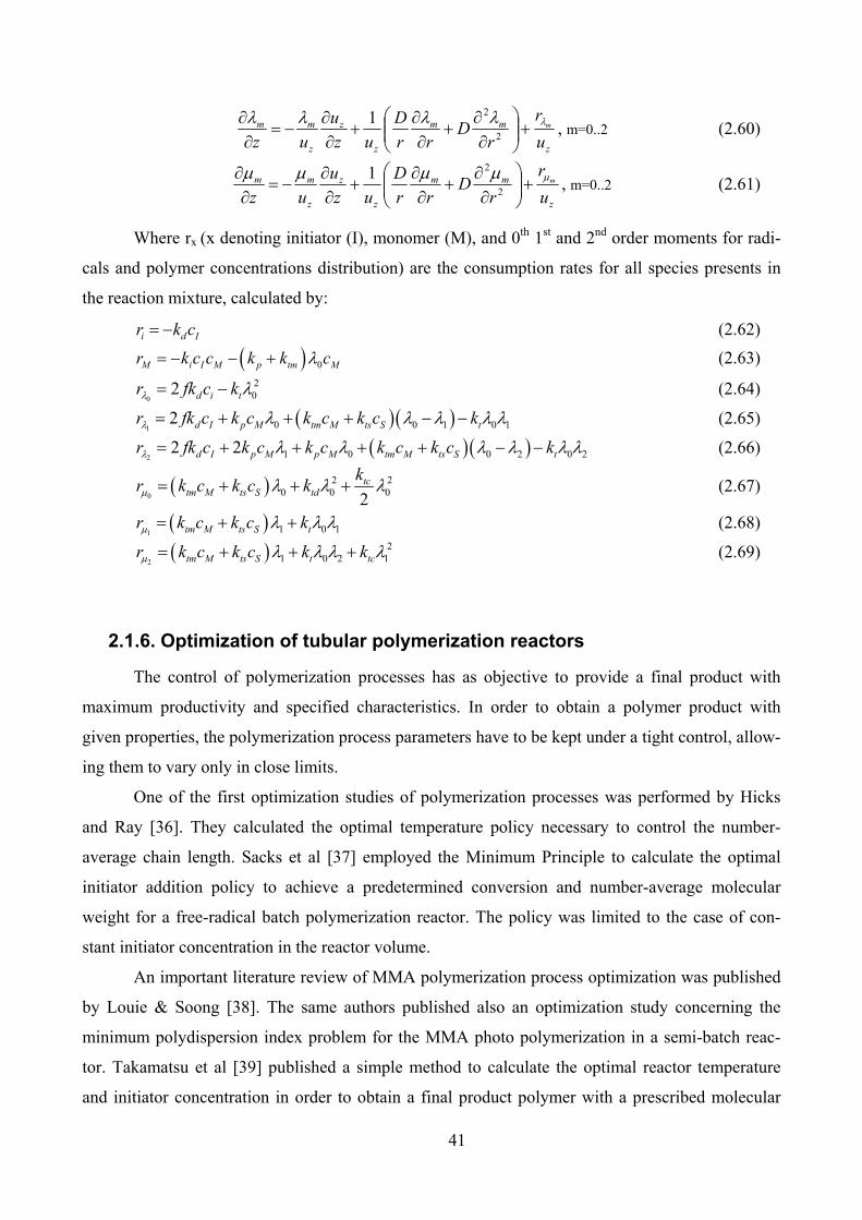
41
z
mm
z
z
z
mm
u
r
rD
rr
D
uz
u
uz
mλλλλλ +⎟⎟⎠⎞⎜⎜⎝
⎛∂
∂+∂∂+∂
∂−=∂∂
2
21, m=0..2 (2.60)
z
mm
z
z
z
mm
u
r
rD
rr
D
uz
u
uz
mμμμμμ +⎟⎟⎠⎞⎜⎜⎝
⎛∂
∂+∂∂+∂
∂−=∂∂
2
21, m=0..2 (2.61)
Where rx (x denoting initiator (I), monomer (M), and 0th 1st and 2nd order moments for radi-
cals and polymer concentrations distribution) are the consumption rates for all species presents in
the reaction mixture, calculated by:
i d Ir k c= − (2.62) ( ) 0M i I M p tm Mr k c c k k cλ= − − + (2.63)
0
202 d i tr fk c kλ λ= − (2.64)
( )( )1 0 0 1 0 12 d I p M tm M ts S tr fk c k c k c k c kλ λ λ λ λ λ= + + + − − (2.65)
( )( )2 1 0 0 2 0 22 2d I p M p M tm M ts S tr fk c k c k c k c k c kλ λ λ λ λ λ λ= + + + + − − (2.66)
( )0
2 20 0 02
tctm M ts S td
kr k c k c kμ λ λ λ= + + + (2.67)
( )1 1 0 1tm M ts S tr k c k c kμ λ λ λ= + + (2.68)
( )2
21 0 2 1tm M ts S t tcr k c k c k kμ λ λ λ λ= + + + (2.69)
2.1.6. Optimization of tubular polymerization reactors
The control of polymerization processes has as objective to provide a final product with
maximum productivity and specified characteristics. In order to obtain a polymer product with
given properties, the polymerization process parameters have to be kept under a tight control, allow-
ing them to vary only in close limits.
One of the first optimization studies of polymerization processes was performed by Hicks
and Ray [36]. They calculated the optimal temperature policy necessary to control the number-
average chain length. Sacks et al [37] employed the Minimum Principle to calculate the optimal
initiator addition policy to achieve a predetermined conversion and number-average molecular
weight for a free-radical batch polymerization reactor. The policy was limited to the case of con-
stant initiator concentration in the reactor volume.
An important literature review of MMA polymerization process optimization was published
by Louie & Soong [38]. The same authors published also an optimization study concerning the
minimum polydispersion index problem for the MMA photo polymerization in a semi-batch reac-
tor. Takamatsu et al [39] published a simple method to calculate the optimal reactor temperature
and initiator concentration in order to obtain a final product polymer with a prescribed molecular
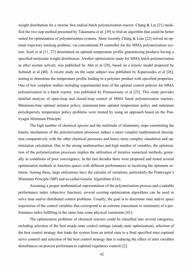
42
weight distribution for a styrene free-radical batch polymerization reactor. Chang & Lai [21] modi-
fied the two step method presented by Takamatsu et al. [39] to find an algorithm that could be better
suited for optimization of polymerization systems. More recently Chang & Liao [22] solved an op-
timal trajectory tracking problem, via conventional PI controller for the MMA polymerization sys-
tem. Scali et al [11, 27] determined an optimal temperature profile guaranteeing products having a
specified molecular weight distribution. Another optimization study for MMA batch polymerization
in ethyl acetate solvent, was published by Ahn et al [20], based on a kinetic model proposed by
Schmidt et al [40]. A recent study on the same subject was published by Kiparissides et al [26],
aiming to determine the temperature profile leading to a polymer product with specified properties.
One of few complete studies including experimental tests of the optimal control policies for MMA
polymerization in a batch reactor, was published by Ponnuswamy et al [23]. This study provides
detailed analysis of open-loop and closed-loop control of MMA batch polymerization reactors.
Minimum-time optimal initiator policy, minimum-time optimal temperature policy and minimum
polydispersity temperature policy problems were treated by using an approach based on the Pon-
tryagin Minimum Principle.
The high number of chemical species and the multitude of elementary steps constituting the
kinetic mechanism of the polymerization processes induce a more complex mathematical descrip-
tion comparatively with the other chemical processes and hence more complex simulation and op-
timization calculation. Due to the strong nonlinearities and high number of variables, the optimiza-
tion of the polymerization processes implies the utilization of iterative numerical methods, gener-
ally in conditions of poor convergence. In the last decades there were proposed and tested several
optimization methods in function spaces with different performances in localizing the optimum so-
lution. Among these, large utilizations have the calculus of variations, particularly the Pontryagin’s
Minimum Principle (MP) and so-called Genetic Algorithms (GA).
Assuming a proper mathematical representation of the polymerization process and a suitable
performance index (objective function), several existing optimization algorithms can be used to
solve time and/or distributed control problems. Usually, the goal is to determine time and/or space
trajectories of the control variables that correspond to an extreme (maximum or minimum) of a per-
formance index fulfilling in the same time some physical constraints [41].
The optimization problems of chemical reactors could be classified into several categories,
including selection of the best steady-state control settings (steady-state optimization), selection of
the best control strategy that leads the system from an initial state to a final specified state (optimal
servo control) and selection of the best control strategy that is reducing the effect of inlet variables
disturbances on process performances (optimal regulatory control) [2].

43
The mathematical model of a polymerization tubular reactor could be written in a general
formulation as [42, 43]:
( ) ( )( ) ( )0 0 0, , , ,f
dxf x z u z z x z x z z z
dz= = ≤ ≤ (2.70)
Where x and u are vectors of state and control variables respectively, and z the reactor axial
coordinate.
The optimization problem consists in finding a control u* that leads the system from an ini-
tial state x0 at z=z0 to a final state xf at z=zf, so that to minimize the performance index:
( )( ) ( ) ( )( )0
, , ,fz
f fz
J h x z z g x u dτ τ τ τ= + ∫ (2.71)
In the case of terminal control problems the performance index is written:
( ) ( ) ( )( )2
,1
, or ,N
i f i d f f f
i
J x z x z J h x z z=
⎡ ⎤= − =⎣ ⎦∑ (2.72)
When the states xi have different orders of magnitude, each term in the performance index
(2.72) is multiplied by a weighting coefficient, in order to bring the values of all terms at the same
order of magnitude. Considering a polymerization process where the objective is to realize imposed
final values for monomer conversion, number-average molecular weight and polydispersion index,
the performance index has the expression:
( ) ( )( ) ( )( )2 22
1 , 2 , 3( )M f M d n f n d f dJ w X z X w M z M w IP z IP= − + − + − (2.73)
With XM – monomer conversion, Mn – number-average molecular weight, IP – polydisper-
sion index and index d denoting the imposed values of the process variables. The values of weight-
ing coefficients, wi, will be discussed separately for each optimization problem.
Pontryagin’s Minimum Principle (MP)
One of the classical methods in solving the optimal control problems is the Pontryagin’s
Minimum Principle. The Minimum Principle states that a optimal control policy, u*(z), that is
minimizing the performance index (2.71), is minimizing in the same time the ‘Hamiltonian func-
tional’ of the problem, defined by the expression [41]:
( ) ( ) ( )( ) ( ) ( )( ) ( ) ( )( )H , , , , , , ,Tx z u z p z z g x z u z z p f x z u z z⎡ ⎤= + ⎣ ⎦ (2.74)
Mathematically, the principle is written:
( ) ( ) ( ) ( ) ( )( )* *min J min H , , ,u t u t
x z u z p z z= (2.75)
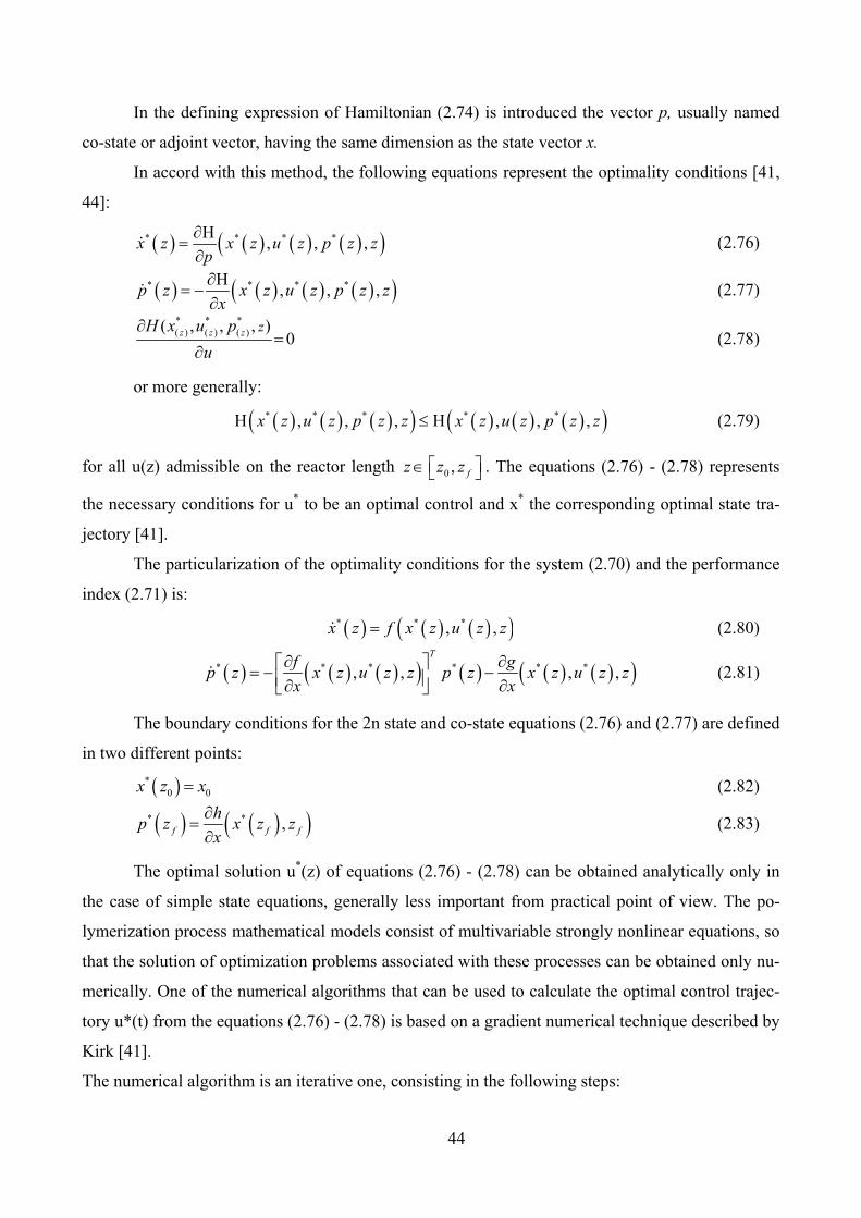
44
In the defining expression of Hamiltonian (2.74) is introduced the vector p, usually named
co-state or adjoint vector, having the same dimension as the state vector x.
In accord with this method, the following equations represent the optimality conditions [41,
44]:
( ) ( ) ( ) ( )( )* * * *H, , ,x z x z u z p z z
p
∂= ∂& (2.76)
( ) ( ) ( ) ( )( )* * * *H, , ,p z x z u z p z z
x
∂= − ∂& (2.77)
* * *( ) ( ) ( )( , , , )
0z z z zH x u p
u
∂ =∂ (2.78)
or more generally:
( ) ( ) ( )( ) ( ) ( ) ( )( )* * * * *H , , , H , , ,x z u z p z z x z u z p z z≤ (2.79)
for all u(z) admissible on the reactor length 0 , fz z z⎡ ⎤∈ ⎣ ⎦ . The equations (2.76) - (2.78) represents
the necessary conditions for u* to be an optimal control and x* the corresponding optimal state tra-
jectory [41].
The particularization of the optimality conditions for the system (2.70) and the performance
index (2.71) is:
( ) ( ) ( )( )* * *, ,x z f x z u z z=& (2.80)
( ) ( ) ( )( ) ( ) ( ) ( )( )* * * * * *, , , ,T
f gp z x z u z z p z x z u z z
x x
∂ ∂⎡ ⎤= − −⎢ ⎥∂ ∂⎣ ⎦& (2.81)
The boundary conditions for the 2n state and co-state equations (2.76) and (2.77) are defined
in two different points:
( )*0 0x z x= (2.82)
( ) ( )( )* * ,f f f
hp z x z z
x
∂= ∂ (2.83)
The optimal solution u*(z) of equations (2.76) - (2.78) can be obtained analytically only in
the case of simple state equations, generally less important from practical point of view. The po-
lymerization process mathematical models consist of multivariable strongly nonlinear equations, so
that the solution of optimization problems associated with these processes can be obtained only nu-
merically. One of the numerical algorithms that can be used to calculate the optimal control trajec-
tory u*(t) from the equations (2.76) - (2.78) is based on a gradient numerical technique described by
Kirk [41].
The numerical algorithm is an iterative one, consisting in the following steps:

45
• Initialize an iteration index, k = 0. Guess a starting control function ( ) ( )ku z , integrate equa-
tions (2.70) from 0 to zf and store the calculated state variables values;
• Using the final values for the monomer state variables stored at step (a) calculate final
boundary conditions for the variables pi, by (2.83), integrate differential equations (2.70)
and calculate the gradient of the Hamiltonian:
( ) ( )
u
fp
u
H kT
k
∂∂=∂
∂ (2.84)
• Adjust the optimal control variable profile on the Hamiltonian gradient direction:
( )( ) ( )( ) ( )( )kkk
u
zHzuzu ∂
∂−=+ λ1 (2.85)
(λ – a small real number used as iteration step);
• Integrate the state equations (2.70) for the new control variable profile, u(z)(k+1) and the new
value of the performance index, J(k+1);calculate the improvement of the performance index:
( ) ( )
( )k
kk
J
JJ −=Δ +1
(2.86)
• Increment the iteration index k and continue with step a, until Δ ≤ i.
Usually, the value of the iteration step, λ , is selected at each iteration, k, by an unidirec-
tional search procedure, so as to minimize the performance index value J(k) on the corresponding
Hamiltonian gradient profile, ( ) ( )k
H z
u
∂∂ . A drawback of this algorithm, especially for highly nonlin-
ear and multivariable processes is its poor convergence to the global optimum and the strong de-
pendence of this convergence on the guess of starting control function u(0)(z).
Consequently, the success in application of the Pontryagin’s Minimum Principle is strongly
dependent on the process model complexity. It is very convenient for the processes described by a
reasonable number of equations in the process model.
The Genetic Algorithms
When the number of state and control variables is important and the process features a high
nonlinearity, the optimization methods from the class of evolutionary algorithms are more efficient
in the localization of global minimum of the performance index. In the last several years, the so-

46
called Genetic Algorithms (GA) has gained wide acceptance as a robust optimization algorithm in
almost all areas of science and engineering. Polymer science and engineering is no exception. Fur-
thermore, multiple-objective functions have been optimized simultaneously by this method. Chak-
ravarthy et al [45] and Lee et al [46] were among the first to adapt simple GA and use it to optimize
polymer production using decision variables that are continuous functions of time. Chakravarthy et
al [47] studied the optimization of the bulk polymerization of MMA. This is an interesting and
complex system because it exhibits the gel effect, which is associated with an extremely sharp in-
crease in the monomer conversion with time at some stage of polymerization. They used the tem-
perature history to minimize the reaction time in a batch reactor while simultaneously requiring the
attainment of the design values (monomer conversion and degree of polymerization).
Lee et al [46] carried out a similar time-optimal control of a continuous-flow stirred in
which random copolymerization of MMA and vinyl alcohol was taking place, during startup or
grade-change. The system does not shows the Trommsdorf effect but is quite complex because of
the simultaneous polymerization of the two monomers. They calculated the optimal jacket tempera-
ture history and the history of the flow rate of VA to minimize the transition time. At the same time,
they used two end-point constraints: the polymer product was forced to be of a desired molecular
weight and the average mole fraction of VA in the polymer product was to have a desired value.
Some of the advantages of a GA include the following: optimizes with continuous or dis-
crete variables, doesn’t require derivative information, simultaneously searches from a wide sam-
pling of the cost surface, can deal with a large number of variables, is well suited for parallel com-
puters, optimizes variables with extremely complex cost surfaces (they can jump out of a local min-
imum), provides a list of optimum variables, not just a single solution, may encode the variables so
that the optimization is done with the en-coded variables, works with numerically generated data,
experimental data, or analytical functions.
A standard genetic algorithm consists in the following steps [43, 48]:
Ü Generate an initial set of control policies (profiles) P(0) at random and set iteration in-
dex, i = 0;
Ü Evaluate the performances of all control profiles in the set P(0) and sort them in respect
with performance index values, J;
REPEAT
Ü Select the best PK profiles in the initial set P(0);
Ü Make reciprocal changes of Nc elements between pairs of selected profiles (Nc ran-
domly calculated);
47
Ü Randomly alterate certain values of the control variables (mutation) obtain next gen-
eration P(i+1);
UNTIL the stop criterion is satisfied.
The principle of the GA we used was taken from the literature [48] and adapted to solve po-
lymerization tubular reactor optimization problem. As example, consider an optimization problem
involving a temperature profile as control variable. The GA optimization calculus is initialized with
a set of S temperature profiles, ( )0iP , i=1,..S, (as defined in the expressions (2.87) below), each one
consisting of N temperature values along the reactor. Then, the quality of each temperature profile
is evaluated by the performance index value and the profiles are sorted in respect with these val-
ues ( ) ( ) ( )( )0 0 01 2 ... SJ J J< < .
Further, an iterative selection procedure is applied. The best K = S×Pselect temperature pro-
files ( )k
iP are chosen to be used in the next step as “parent” solutions, where Pselect is the “probability
of selection”. These best K temperature profiles are kept for the next „generation”, the other S-K
being replaced by new “children profiles”.
( ) ( ) ( ) ( ) ( ) ( )[ ]( ) ( ) ( ) ( ) ( ) ( )[ ]( ) ( ) ( ) ( ) ( ) ( )[ ]0,0,
10,
30,
20,
10
0,0,1
0,3
0,2
0,1
0
0,10,11
0,13
0,12
0,11
01
....
.........................................................
....
........................................................
....
S
N
S
N
SSS
S
i
N
i
N
iii
i
NN
TTTTTP
TTTTTP
TTTTTP
−
−
−
=
=
=
(2.87)
A „crossover operator” is responsible for the information exchange between „parent” solu-
tions, in order to generate „children” solutions. To apply the specified crossover operator, there are
randomly chosen pairs of “parent” profiles among the selected K profiles. For example, the “parent”
profiles (2.88) will generate another two “children” profiles, (2.89), that will replace two of the
worst (S-K) profiles in the hierarchy.
( ) ( ) ( ) ( ) ( ) ( )[ ] ( ) ( ) ( ) ( ) ( ) ( )[ ][ ];K,l,mwhere
;TT....TTTP;TT....TTTP m,k
N
m,k
N
m,km,km,kk
m
l,k
N
l,k
N
l,kl,kl,kk
l
113211321
∈== −− (2.88)
( ) ( ) ( ) ( ) ( ) ( ) ( ) ( )[ ]( ) ( ) ( ) ( ) ( ) ( ) ( ) ( )[ ]l,k
N
l,k
j
l,k
j
m,k
j
m,km,km,kk
m
m,k
N
m,k
j
m,k
j
l,k
j
l,kl,kl,kk
l
..TTT....TTTTP
..TTT....TTTTP
213211
213211
++++++
==
(2.89)
On overall, a number of (S-K)/2 such crossover operations between randomly chosen pairs
of temperature profiles from the set K will be performed to generate the “child” solutions. Further, a
„mutation operator” is used in order to perform random changes on the values of elements con-
tained in the selected set of S temperature profiles. The number of random changes is given by
48
mutM S N P= ⋅ ⋅ , where Pmut is the “probability of mutation” chosen in this study 10-3, similar value
with those published by Kennedy et al [49] and Marco et al [50] . The random “mutation” of a cer-
tain temperature value in the profile i at iteration k follows the relation:
( ) ( ) ( ) ( )NjSiTaT ki
j
ki
j ,1,,1,1,, ∈∈⋅= − (2.90)
where a are randomly generated numbers in the range (0, 1).
The procedure of evaluation of the temperature profiles qualities continues with the new set
so obtained and a new ‘family’ of parents and children profiles is generated in the same manner. By
iterating, the set P(i) of temperature profiles is evaluating toward better and better performances.
Finally, the temperature profile fulfilling the demanded minimization of performance index is iden-
tified. The same principle is used in the case of other control variables.
As expected, the algorithm performances (accuracy of global optimum localization and the
associated computation time) are depending on the size of explored temperature interval, the num-
ber of the points defining a temperature profile, N, the number of profiles S and K involved in im-
provement iterations, as well as the constants Pselect, Pmut and a. The identification of the best values
of these algorithm parameters is a matter of exploratory calculation trials that is burdening the op-
timization calculus.
2.2. Simulation of a tubular reactor for MMA polymerization in solu-
tion
In order to underline the main features of the polymerization process taking place in tubular
reactors, several simulation studies will be presented, before to approach the optimization problems,
based on plug flow and laminar flow models. A comparison of the results provided by the two flow
models will be then discussed.
2.2.1. Selection of the kinetic model
To select an appropriate kinetic model for the MMA solution polymerization process, simu-
lation of a plug-flow reactor were performed in identical operating conditions, using the rate con-
stants proposed by different authors, presented in Table 2.4. The simulations were performed con-
sidering the working conditions specified in Table 2.5 and the assumptions of constant density, neg-
ligible gel effect on the propagation and termination steps and isothermal operating regime.
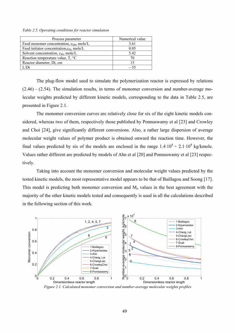
49
Table 2.5. Operating conditions for reactor simulation
Process parameter Numerical value Feed monomer concentration, cM0, mole/L 3.61 Feed initiator concentration,cI0, mole/L 0.05 Solvent concentration, cS0, mole/L 5.42 Reaction temperature value, T, °C 70 Reactor diameter, Dt, cm 15 L/Dt ~ 55
The plug-flow model used to simulate the polymerization reactor is expressed by relations
(2.46) - (2.54). The simulation results, in terms of monomer conversion and number-average mo-
lecular weights predicted by different kinetic models, corresponding to the data in Table 2.5, are
presented in Figure 2.1.
The monomer conversion curves are relatively close for six of the eight kinetic models con-
sidered, whereas two of them, respectively those published by Ponnuswamy et al [23] and Crowley
and Choi [24], give significantly different conversions. Also, a rather large dispersion of average
molecular weight values of polymer product is obtained onward the reaction time. However, the
final values predicted by six of the models are enclosed in the range 1.4·104 ÷ 2.1·104 kg/kmole.
Values rather different are predicted by models of Ahn et al [20] and Ponnuswamy et al [23] respec-
tively.
Taking into account the monomer conversion and molecular weight values predicted by the
tested kinetic models, the most representative model appears to be that of Baillagou and Soong [17].
This model is predicting both monomer conversion and Mn values in the best agreement with the
majority of the other kinetic models tested and consequently is used in all the calculations described
in the following section of this work.
Figure 2.1. Calculated monomer conversion and number-average molecular weights profiles
0 0.2 0.4 0.6 0.8 10
0.2
0.4
0.6
0.8
1
Dimensionless reactor length
Mo
no
me
r co
nve
rsio
n
1-Baillagou
2-Kiparissides
3-Ahn
4-Chang, Lai
5-ChangLiao
6-CrowleyChoi
7-Scali
8-Ponnuswamy
1, 2, 4, 5, 7
3
68
0 0.2 0.4 0.6 0.8 10
1
2
3
4
5
6
7x 10
4
Dimensionless reactor length
Nu
mb
er-
ave
rag
e m
ole
cu
lar
we
igh
t, k
g/k
mo
le
1-Baillagou
2-Kiparissides
3-Ahn
4-Chang, Lai
5-ChangLiao
6-CrowleyChoi
7-Scali
8-Ponnuswamy
8
7
41
25
6
3
50
2.2.2. Simulation of the laminar flow polymerization reactor
In this paragraph will be analyzed the behavior of a laminar-flow reactor in different oper-
ating conditions. In this aim, a simulation calculus is performed based on the kinetic model selected
above (Baillagou and Soong [16, 17]). The gel effect is described by the model proposed by Chiu et
al [13], the constitutive equations being presented in Table 2.2. The characteristics of the reactor are
displayed in Table 2.6. Because of the strong exothermicity of the polymerization process, a high
value of length to diameter ratio is chosen, insuring a high specific heat transfer area.
Table 2.6. Tubular reactor characteristics
Process parameter Numerical value Total mass flow rate / [kg/s] 10-3 Feed initiator concentration (cI0) / [mole/L] 0.05 Toluene mass fraction in the feed 0.5 Reactor length / [m] 8 Reactor diameter (dt) / [m] 2×10⁻² Feed temperature / [OC] 80 Thermal agent temperature / [OC] 80
The reactor model was presented in paragraph 2.1.5. The radial convection terms are ig-
nored in the model, this being explained by the high length to diameter ratio of the reactor. In the
axial direction, mass diffusion and heat conduction are assumed to be negligible as compared to the
convective terms.
Variations of monomer conversion and consequently of mixture viscosity and density pro-
duce strong radial variations in the axial velocities. The flow is considered fully developed at the
reactor entrance and the velocity profiles along the reactor axis are calculated using the method
proposed by Lynn and Huff [32]. The physical properties (density, viscosity, thermal conductivity)
of the reaction mixture are estimated using relations published in literature [2, 7, 17, 18].
It is considered that the main resistance to the heat transfer in radial direction occurs inside
the reactor. Therefore, the overall heat transfer coefficient, U, is approximated by the internal partial
heat transfer coefficient calculated by the equation (2.91), where the variation of the viscosity at the
wall proximity is neglected (the ratio / pη η approaches unity) [51]:
0.140.8
0.467
0.193.66
1 0.177t
p
d GzNu
k Gz
α ηη
⎛ ⎞= = + ⎜ ⎟⎜ ⎟+ ⎝ ⎠ (2.91)
Where Gz is the Graetz number, defined by Re PrtdGz
L= , with Re – Reynolds number and
Pr – Prandtl number. In the energy balance, as generally accepted, only the heat generated in
propagation reactions and chain transfer to monomer is considered [16, 17], so that the heat genera-
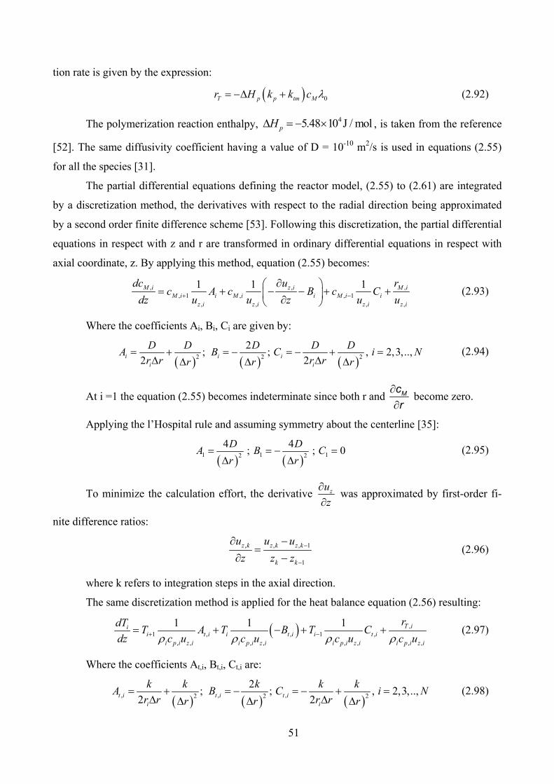
51
tion rate is given by the expression:
( ) 0T p p tm Mr H k k c λ= −Δ + (2.92)
The polymerization reaction enthalpy, 45.48 10 J / molpHΔ = − × , is taken from the reference
[52]. The same diffusivity coefficient having a value of D = 10-10 m2/s is used in equations (2.55)
for all the species [31].
The partial differential equations defining the reactor model, (2.55) to (2.61) are integrated
by a discretization method, the derivatives with respect to the radial direction being approximated
by a second order finite difference scheme [53]. Following this discretization, the partial differential
equations in respect with z and r are transformed in ordinary differential equations in respect with
axial coordinate, z. By applying this method, equation (2.55) becomes:
, , ,, 1 , , 1
, , , ,
1 1 1M i z i M i
M i i M i i M i i
z i z i z i z i
dc u rc A c B c C
dz u u z u u+ −
∂⎛ ⎞= + − − + +⎜ ⎟∂⎝ ⎠ (2.93)
Where the coefficients Ai, Bi, Ci are given by:
( ) ( ) ( )2 2 2
2; ; , 2,3,..,
2 2= + = − = − + =Δ ΔΔ Δ Δi i i
i i
D D D D DA B C i N
r r r rr r r (2.94)
At i =1 the equation (2.55) becomes indeterminate since both r and ∂∂ Mc
r become zero.
Applying the l’Hospital rule and assuming symmetry about the centerline [35]:
( ) ( )1 1 12 2
4 4; ; 0
D DA B C
r r= = − =Δ Δ (2.95)
To minimize the calculation effort, the derivative zu
z
∂∂ was approximated by first-order fi-
nite difference ratios:
, , , 1
1
z k z k z k
k k
u u u
z z z
−−
∂ −=∂ − (2.96)
where k refers to integration steps in the axial direction.
The same discretization method is applied for the heat balance equation (2.56) resulting:
( ) ,1 , , 1 ,
, , , , , , , ,
1 1 1 T iii t i i t i i t i
i p i z i i p i z i i p i z i i p i z i
rdTT A T B T C
dz c u c u c u c uρ ρ ρ ρ+ −= + − + + (2.97)
Where the coefficients At,i, Bt,i, Ct,i are:
( ) ( ) ( ), , ,2 2 2
2; ; , 2,3,..,
2 2t i t i t i
i i
k k k k kA B C i N
r r r rr r r= + = − = − + =Δ ΔΔ Δ Δ (2.98)
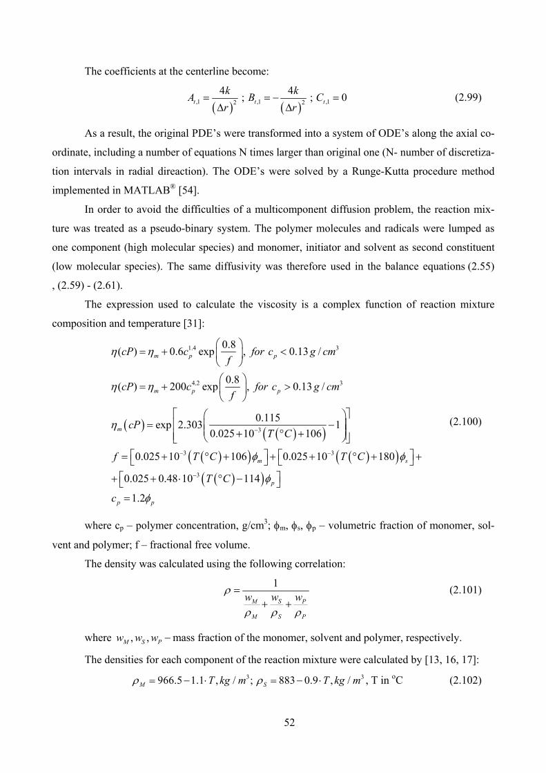
52
The coefficients at the centerline become:
( ) ( ),1 ,1 ,12 2
4 4; ; 0t t t
k kA B C
r r= = − =Δ Δ (2.99)
As a result, the original PDE’s were transformed into a system of ODE’s along the axial co-
ordinate, including a number of equations N times larger than original one (N- number of discretiza-
tion intervals in radial direaction). The ODE’s were solved by a Runge-Kutta procedure method
implemented in MATLAB® [54].
In order to avoid the difficulties of a multicomponent diffusion problem, the reaction mix-
ture was treated as a pseudo-binary system. The polymer molecules and radicals were lumped as
one component (high molecular species) and monomer, initiator and solvent as second constituent
(low molecular species). The same diffusivity was therefore used in the balance equations (2.55)
, (2.59) - (2.61).
The expression used to calculate the viscosity is a complex function of reaction mixture
composition and temperature [31]:
( ) ( )( )( )( ) ( )( )
1.4 3
4.2 3
3
3 3
0.8( ) 0.6 exp , 0.13 /
0.8( ) 200 exp , 0.13 /
0.115exp 2.303 1
0.025 10 106
0.025 10 106 0.025 10 180
0.02
m p p
m p p
m
m s
cP c for c g cmf
cP c for c g cmf
cPT C
f T C T C
η ηη η
ηφ φ−
− −
⎛ ⎞= + <⎜ ⎟⎝ ⎠⎛ ⎞= + >⎜ ⎟⎝ ⎠
⎡ ⎤⎛ ⎞= −⎢ ⎥⎜ ⎟⎜ ⎟+ ° +⎢ ⎥⎝ ⎠⎣ ⎦⎡ ⎤ ⎡ ⎤= + ° + + + ° + +⎣ ⎦ ⎣ ⎦
+ ( )( )35 0.48 10 114
1.2
p
p p
T C
c
φφ
−⎡ ⎤+ ⋅ ° −⎣ ⎦=
(2.100)
where cp – polymer concentration, g/cm3; φm, φs, φp – volumetric fraction of monomer, sol-
vent and polymer; f – fractional free volume.
The density was calculated using the following correlation:
1
SM P
M S P
ww wρ
ρ ρ ρ=
+ + (2.101)
where , ,M S Pw w w − mass fraction of the monomer, solvent and polymer, respectively.
The densities for each component of the reaction mixture were calculated by [13, 16, 17]:
3 3966.5 1.1 , / ; 883 0.9 , /M ST kg m T kg mρ ρ= − ⋅ = − ⋅ , T in oC (2.102)
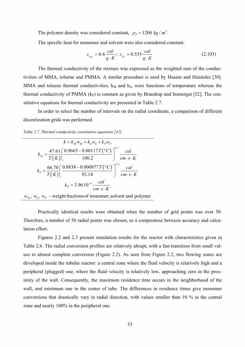
53
The polymer density was considered constant, 31200 /P kg mρ = .
The specific heat for monomer and solvent were also considered constant:
0.4 ; 0.535M Sp p
cal calc c
g K g K= =⋅ ⋅ (2.103)
The thermal conductivity of the mixture was expressed as the weighted sum of the conduc-
tivities of MMA, toluene and PMMA. A similar procedure is used by Husain and Hamielec [30].
MMA and toluene thermal conductivities, kM and kS, were functions of temperature whereas the
thermal conductivity of PMMA (kP) is constant as given by Brandrup and Immergut [52]. The con-
stitutive equations for thermal conductivity are presented in Table 2.7.
In order to select the number of intervals on the radial coordinate, a comparison of different
discretization grids was performed.
Table 2.7. Thermal conductivity constitutive equations [31]
M M S S P Pk k w k w k w= + +
( ) ( ) 4/30.9665 0.0011747.61
100.2M
T C calk
T K cm s K
− °⎛ ⎞= ⎜ ⎟ ⋅ ⋅⎝ ⎠
( ) ( ) 4 /30.8838 0.00087766.70
92.14S
T C calk
T K cm s K
− °⎛ ⎞= ⎜ ⎟ ⋅ ⋅⎝ ⎠ 43.9610P
calk
cm s K
−= ⋅ ⋅
, , weight fractionsof monomer,solvent and polymerM S Pw w w −
Practically identical results were obtained when the number of grid points was over 50.
Therefore, a number of 50 radial points was chosen, as a compromise between accuracy and calcu-
lation effort.
Figures 2.2 and 2.3 present simulation results for the reactor with characteristics given in
Table 2.6. The radial conversion profiles are relatively abrupt, with a fast transition from small val-
ues to almost complete conversion (Figure 2.2). As seen from Figure 2.2, two flowing zones are
developed inside the tubular reactor: a central zone where the fluid velocity is relatively high and a
peripheral (plugged) one, where the fluid velocity is relatively low, approaching zero in the prox-
imity of the wall. Consequently, the maximum residence time occurs in the neighborhood of the
wall, and minimum one in the center of tube. The differences in residence times give monomer
conversions that drastically vary in radial direction, with values smaller than 10 % in the central
zone and nearly 100% in the peripheral one.
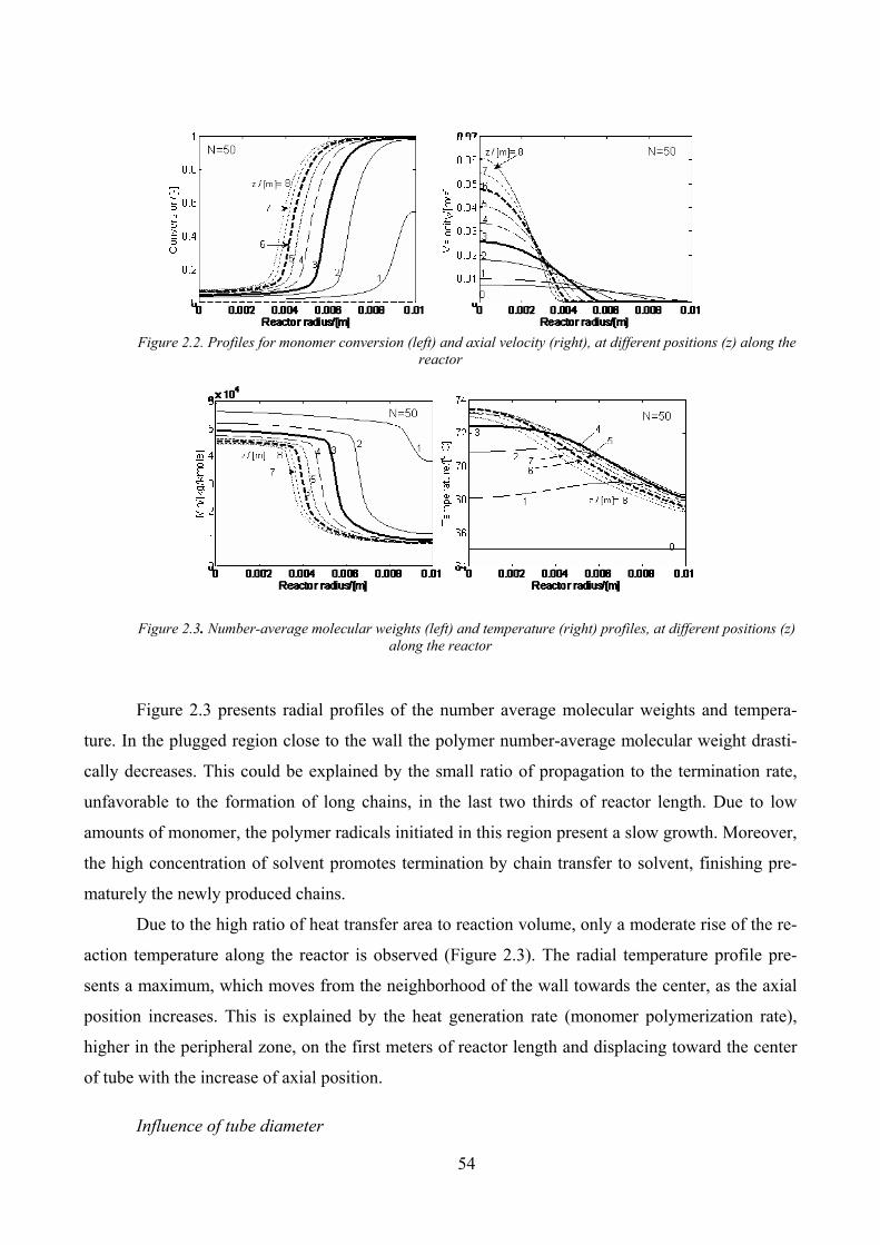
54
Figure 2.2. Profiles for monomer conversion (left) and axial velocity (right), at different positions (z) along the
reactor
Figure 2.3. Number-average molecular weights (left) and temperature (right) profiles, at different positions (z)
along the reactor
Figure 2.3 presents radial profiles of the number average molecular weights and tempera-
ture. In the plugged region close to the wall the polymer number-average molecular weight drasti-
cally decreases. This could be explained by the small ratio of propagation to the termination rate,
unfavorable to the formation of long chains, in the last two thirds of reactor length. Due to low
amounts of monomer, the polymer radicals initiated in this region present a slow growth. Moreover,
the high concentration of solvent promotes termination by chain transfer to solvent, finishing pre-
maturely the newly produced chains.
Due to the high ratio of heat transfer area to reaction volume, only a moderate rise of the re-
action temperature along the reactor is observed (Figure 2.3). The radial temperature profile pre-
sents a maximum, which moves from the neighborhood of the wall towards the center, as the axial
position increases. This is explained by the heat generation rate (monomer polymerization rate),
higher in the peripheral zone, on the first meters of reactor length and displacing toward the center
of tube with the increase of axial position.
Influence of tube diameter
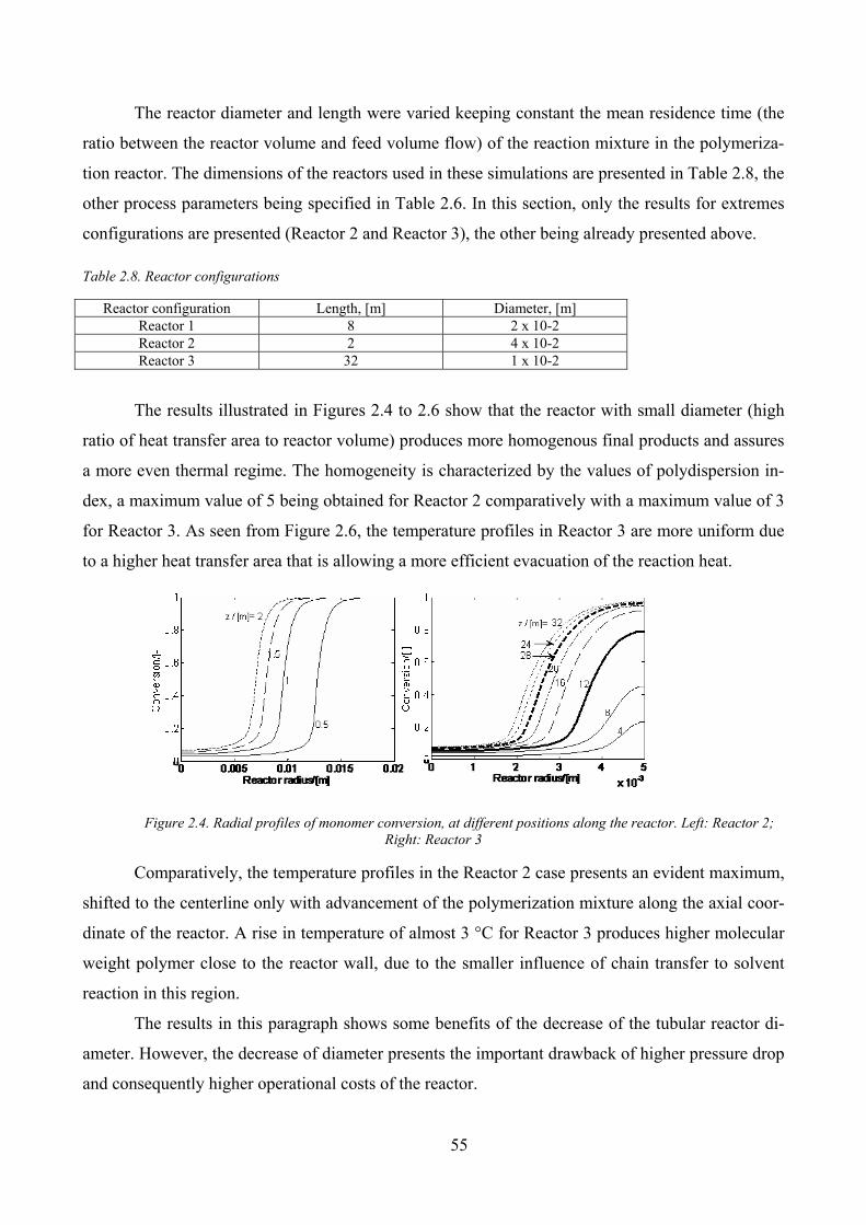
55
The reactor diameter and length were varied keeping constant the mean residence time (the
ratio between the reactor volume and feed volume flow) of the reaction mixture in the polymeriza-
tion reactor. The dimensions of the reactors used in these simulations are presented in Table 2.8, the
other process parameters being specified in Table 2.6. In this section, only the results for extremes
configurations are presented (Reactor 2 and Reactor 3), the other being already presented above.
Table 2.8. Reactor configurations
Reactor configuration Length, [m] Diameter, [m] Reactor 1 8 2 x 10⁻² Reactor 2 2 4 x 10⁻² Reactor 3 32 1 x 10⁻²
The results illustrated in Figures 2.4 to 2.6 show that the reactor with small diameter (high
ratio of heat transfer area to reactor volume) produces more homogenous final products and assures
a more even thermal regime. The homogeneity is characterized by the values of polydispersion in-
dex, a maximum value of 5 being obtained for Reactor 2 comparatively with a maximum value of 3
for Reactor 3. As seen from Figure 2.6, the temperature profiles in Reactor 3 are more uniform due
to a higher heat transfer area that is allowing a more efficient evacuation of the reaction heat.
Figure 2.4. Radial profiles of monomer conversion, at different positions along the reactor. Left: Reactor 2;
Right: Reactor 3
Comparatively, the temperature profiles in the Reactor 2 case presents an evident maximum,
shifted to the centerline only with advancement of the polymerization mixture along the axial coor-
dinate of the reactor. A rise in temperature of almost 3 °C for Reactor 3 produces higher molecular
weight polymer close to the reactor wall, due to the smaller influence of chain transfer to solvent
reaction in this region.
The results in this paragraph shows some benefits of the decrease of the tubular reactor di-
ameter. However, the decrease of diameter presents the important drawback of higher pressure drop
and consequently higher operational costs of the reactor.
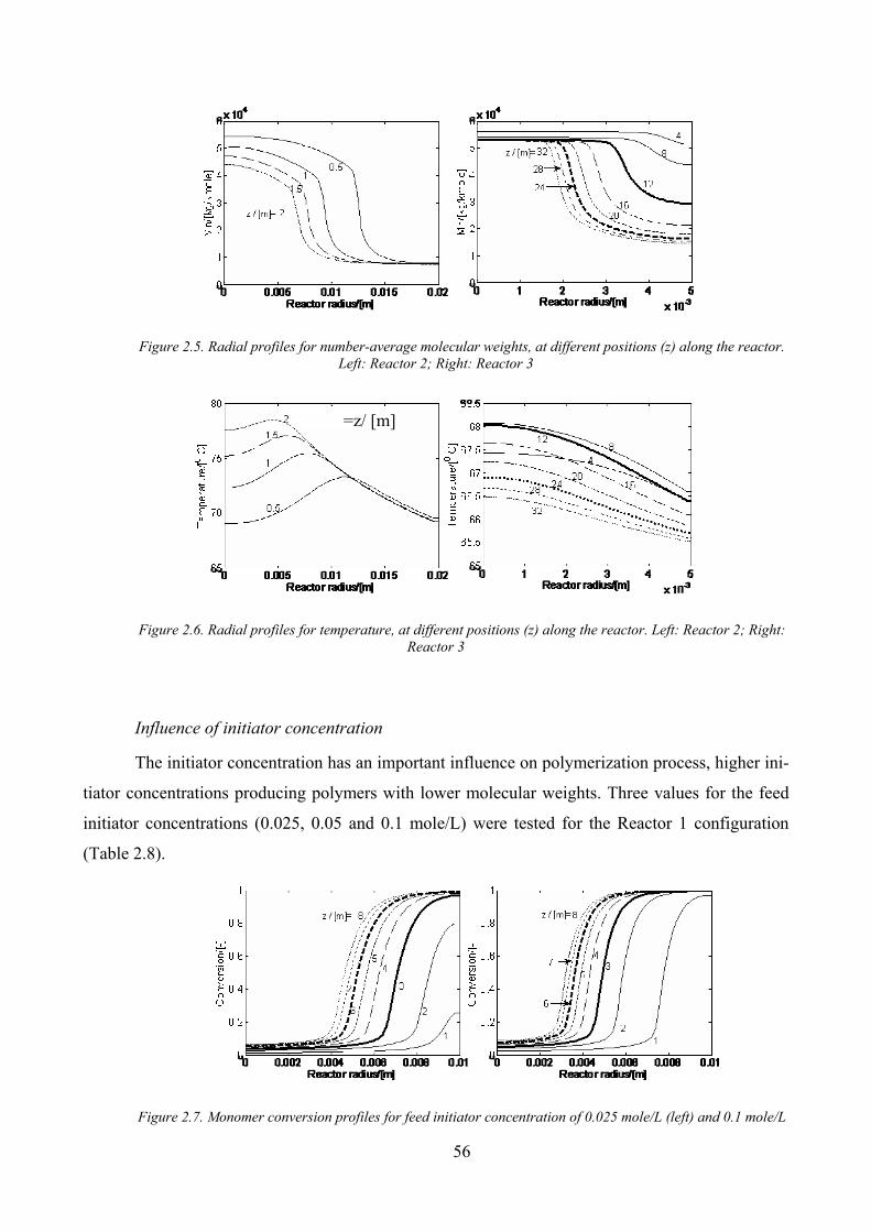
56
Figure 2.5. Radial profiles for number-average molecular weights, at different positions (z) along the reactor.
Left: Reactor 2; Right: Reactor 3
Figure 2.6. Radial profiles for temperature, at different positions (z) along the reactor. Left: Reactor 2; Right:
Reactor 3
Influence of initiator concentration
The initiator concentration has an important influence on polymerization process, higher ini-
tiator concentrations producing polymers with lower molecular weights. Three values for the feed
initiator concentrations (0.025, 0.05 and 0.1 mole/L) were tested for the Reactor 1 configuration
(Table 2.8).
Figure 2.7. Monomer conversion profiles for feed initiator concentration of 0.025 mole/L (left) and 0.1 mole/L
=z/ [m]
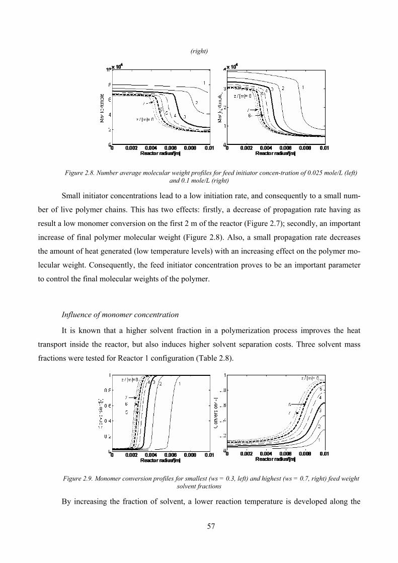
57
(right)
Figure 2.8. Number average molecular weight profiles for feed initiator concen-tration of 0.025 mole/L (left)
and 0.1 mole/L (right)
Small initiator concentrations lead to a low initiation rate, and consequently to a small num-
ber of live polymer chains. This has two effects: firstly, a decrease of propagation rate having as
result a low monomer conversion on the first 2 m of the reactor (Figure 2.7); secondly, an important
increase of final polymer molecular weight (Figure 2.8). Also, a small propagation rate decreases
the amount of heat generated (low temperature levels) with an increasing effect on the polymer mo-
lecular weight. Consequently, the feed initiator concentration proves to be an important parameter
to control the final molecular weights of the polymer.
Influence of monomer concentration
It is known that a higher solvent fraction in a polymerization process improves the heat
transport inside the reactor, but also induces higher solvent separation costs. Three solvent mass
fractions were tested for Reactor 1 configuration (Table 2.8).
Figure 2.9. Monomer conversion profiles for smallest (ws = 0.3, left) and highest (ws = 0.7, right) feed weight
solvent fractions
By increasing the fraction of solvent, a lower reaction temperature is developed along the
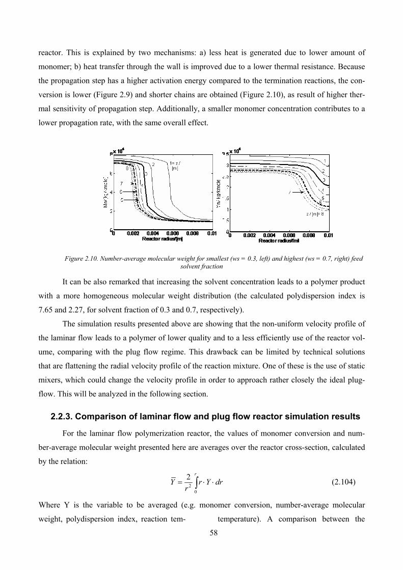
58
reactor. This is explained by two mechanisms: a) less heat is generated due to lower amount of
monomer; b) heat transfer through the wall is improved due to a lower thermal resistance. Because
the propagation step has a higher activation energy compared to the termination reactions, the con-
version is lower (Figure 2.9) and shorter chains are obtained (Figure 2.10), as result of higher ther-
mal sensitivity of propagation step. Additionally, a smaller monomer concentration contributes to a
lower propagation rate, with the same overall effect.
Figure 2.10. Number-average molecular weight for smallest (ws = 0.3, left) and highest (ws = 0.7, right) feed
solvent fraction
It can be also remarked that increasing the solvent concentration leads to a polymer product
with a more homogeneous molecular weight distribution (the calculated polydispersion index is
7.65 and 2.27, for solvent fraction of 0.3 and 0.7, respectively).
The simulation results presented above are showing that the non-uniform velocity profile of
the laminar flow leads to a polymer of lower quality and to a less efficiently use of the reactor vol-
ume, comparing with the plug flow regime. This drawback can be limited by technical solutions
that are flattening the radial velocity profile of the reaction mixture. One of these is the use of static
mixers, which could change the velocity profile in order to approach rather closely the ideal plug-
flow. This will be analyzed in the following section.
2.2.3. Comparison of laminar flow and plug flow reactor simulation results
For the laminar flow polymerization reactor, the values of monomer conversion and num-
ber-average molecular weight presented here are averages over the reactor cross-section, calculated
by the relation:
2
0
2 r
Y r Y drr
= ⋅ ⋅∫ (2.104)
Where Y is the variable to be averaged (e.g. monomer conversion, number-average molecular
weight, polydispersion index, reaction tem- temperature). A comparison between the
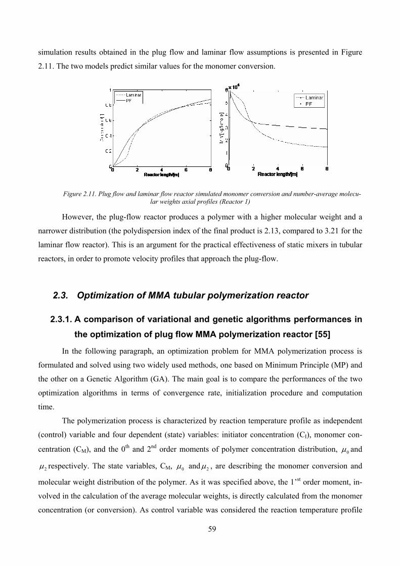
59
simulation results obtained in the plug flow and laminar flow assumptions is presented in Figure
2.11. The two models predict similar values for the monomer conversion.
Figure 2.11. Plug flow and laminar flow reactor simulated monomer conversion and number-average molecu-
lar weights axial profiles (Reactor 1)
However, the plug-flow reactor produces a polymer with a higher molecular weight and a
narrower distribution (the polydispersion index of the final product is 2.13, compared to 3.21 for the
laminar flow reactor). This is an argument for the practical effectiveness of static mixers in tubular
reactors, in order to promote velocity profiles that approach the plug-flow.
2.3. Optimization of MMA tubular polymerization reactor
2.3.1. A comparison of variational and genetic algorithms performances in
the optimization of plug flow MMA polymerization reactor [55]
In the following paragraph, an optimization problem for MMA polymerization process is
formulated and solved using two widely used methods, one based on Minimum Principle (MP) and
the other on a Genetic Algorithm (GA). The main goal is to compare the performances of the two
optimization algorithms in terms of convergence rate, initialization procedure and computation
time.
The polymerization process is characterized by reaction temperature profile as independent
(control) variable and four dependent (state) variables: initiator concentration (CI), monomer con-
centration (CM), and the 0th and 2nd order moments of polymer concentration distribution, 0μ and
2μ respectively. The state variables, CM, 0μ and 2μ , are describing the monomer conversion and
molecular weight distribution of the polymer. As it was specified above, the 1’st order moment, in-
volved in the calculation of the average molecular weights, is directly calculated from the monomer
concentration (or conversion). As control variable was considered the reaction temperature profile
60
T(z). The objective of the problem is to calculate the temperature profile along the reactor that leads
to desired values of polymer properties and monomer conversion at reactor exit, for a given reaction
volume and flow rate (or equivalently, given reaction time). This is accomplished by the minimiza-
tion of the performance index (2.73), where w1, w2 and w3, are weighting factors so chosen, to in-
sure close magnitude orders for all terms of the summation.
The problem so defined could be considered as one of average complexity for a polymeri-
zation process (a single control variable, no heat balance equation necessary in the mathematical
model, plug flow of reaction mixture). More complex problems could be formulated by using more
realistic mathematical models of chemical process and/or considering more control variables (the
temperature of thermal agent along the reactor, the flow rate of thermal agent, the feed flow rate of
reaction mixture and its composition and temperature).
Optimization by Minimum Principle method
The mathematical model of the plug-flow reactor and the optimal conditions were written in
dimensionless variables:
11 1
sd s
z s
zdxk x I f
dz u I= − = (2.105)
( )1/2 1/221 2 1 2
ss s
z s
zdxk x M x I f
dz u M= − = (2.106)
( )( )1/2 1/2 1/2 1/2 232 2 1 3 1 0 3
0
0.5ss s s td tc
z s
dx zk x M x I k Sx I k k f
dz uλμ= + + + = (2.107)
( )( )242 2 1 0 2 4
2
sm s s tc t
z s
zdxk x M k S k k f
dz uλ λ λ λμ= + + + = (2.108)
0 21 2 3 4
0 2
; ; ;s s s s
I Mx x x x
I M
μ μμ μ= = = = (2.109)
The index s is denoting the reference values used in the definitions of dimensionless vari-
ables.
The live polymer distribution moments are:
1/2
2 11 1 00 1 2 1
2 2 0 2
22 2; ;
;
p sd s d s
t
p s s m s t s m s
k x Mfk x I fk x I A
k B B
A k x M k S k M x B k k S k x M
λλλ λ λ λλ
⎛ ⎞ += = = +⎜ ⎟⎝ ⎠= + + = + +
(2.110)
The performance index in dimensionless variables is:
61
( ) ( ) ( )( )( )
2 2 22 2 21 2 2 0, 3 3
2
3 4
2
2
1 1
1;
1
s f d f d
f fd
s f
J w M x w x w IP
x xM
M x
α μ βαα β
= − + − + −−= = −
(2.111)
The optimality conditions (2.76) - (2.78) can be easily particularized for the present optimi-
zation problem. The co-state (adjoint) equations (2.83) are particularized as:
31 1 2 41 2 3 4
1 1 1 1 1
fdp f f fHp p p p
dz x x x x x
⎛ ⎞∂∂ ∂ ∂∂= − = − + + +⎜ ⎟∂ ∂ ∂ ∂ ∂⎝ ⎠ (2.112)
32 1 2 41 2 3 4
2 2 2 2 2
fdp f f fHp p p p
dz x x x x x
⎛ ⎞∂∂ ∂ ∂∂= − = − + + +⎜ ⎟∂ ∂ ∂ ∂ ∂⎝ ⎠ (2.113)
3 31 2 41 2 3 4
3 3 3 3 3
dp ff f fHp p p p
dz x x x x x
⎛ ⎞∂∂ ∂ ∂∂= − = − + + +⎜ ⎟∂ ∂ ∂ ∂ ∂⎝ ⎠ (2.114)
34 1 2 41 2 3 4
4 4 4 4 4
fdp f f fHp p p p
dz x x x x x
⎛ ⎞∂∂ ∂ ∂∂= − = − + + +⎜ ⎟∂ ∂ ∂ ∂ ∂⎝ ⎠ (2.115)
With the boundary conditions at the reactor exit described by:
( )11
0f
f
z z
Jp z
x =∂= =∂ (2.116)
( ) ( ) ( )2 22 1 2 3
2 2
2 2 1f
f s f d
z z
Jp z M x IP
x x
βω α ω β=
∂ ∂= = − + −∂ ∂ (2.117)
( ) ( ) ( )2 23 2 0 3 3
3 3
2 1 2 1f
f d f d
z z
Jp z x IP
x x
βω μ ω β=
∂ ∂= = − + −∂ ∂ (2.118)
( ) ( )24 3
4 4
2 1f
f d
fz z
Jp z IP
x x
βω β=
∂= = −∂ (2.119)
The Hamiltonian derivative in respect with the control variable (in this case the temperature)
necessary in relation (2.85) is:
31 2 41 2 3 4
ff f fHp p p p
T T T T T
∂∂ ∂ ∂∂ = + + +∂ ∂ ∂ ∂ ∂ (2.120)
The derivatives of the functions fi, i = 1..4 in respect with the temperature are:
11
s ds
z s
z dkfx I
T u I dT
∂ = −∂ (2.121)
( )1/2 1/22 12 1
ss s
z s
zf dkx M x I
T u M dT
∂ = −∂ (2.122)
( )1/ 2 1/ 2 1/ 2 1/ 2 23 3 02
2 1 1 0 0
0
0.5 2 0.5∂ ∂= + + + + +∂ ∂
⎛ ⎛ ⎞ ⎞⎜ ⎜ ⎟ ⎟⎝ ⎝ ⎠ ⎠s td tc
s s s td tc
z s
f z dk dk dkdkx M x I Sx I k k
T u dT dT dT dT T
λλ λμ (2.123)

62
( ) 22 12 2 2 1 1
4
2 0 20 2 2 0
2m s tcs m s s tc
s
z s tt t
dk dk dkx M S k x M k S k
zf dT dT T dT T
T u dkk k
dT T T
λ λλ λ λμ λ λλ λ λ λ
⎛ ⎞∂ ∂⎛ ⎞+ + + + +⎜ ⎟⎜ ⎟∂ ∂ ∂⎝ ⎠⎜ ⎟=∂ ⎜ ⎟∂ ∂+ + +⎜ ⎟∂ ∂⎝ ⎠ (2.124)
The numerical algorithm based on a gradient method used to solve this optimization prob-
lem is presented in paragraph 2.1.6.
The values of the different parameters and the working conditions used in the computation
are given in Tables 2.9 and 2.10. For the problem such defined, finding the initial profile leading to
the global minimum proved to be a rather difficult task. The calculation procedures failed to attain
the global minimum of performance index for constant initial profiles, increasing temperature pro-
files and even certain decreasing profiles.
Several initialization temperature profiles and the corresponding solutions are presented in
Figure 2.12 and Table 2.11. The global minimum was obtained only by initializing the algorithm
with a slowly decreasing profile in the interval 329 – 323 K (profile 5 in Table 2.11 and Figure
2.12). Additionally, it is worth to stress that, besides the starting profile, the minimum value of the
performance index is also dependent on the convergence limit, i.
Table 2.9. Working conditions for reactor optimization
Process parameter Numerical value Feed monomer concentration, cM0, mole/L 3.61 Feed initiator concentration,cI0, mole/L 0.05 Solvent concentration, cS0, mole/L 5.42 Reaction temperature value, T, °C 70 Reactor diameter, Dt, cm 15 L/Dt ~ 55
Table 2.10. Specified values in the performance index expression
The best result reported in Table 2.11 was found with an extremely low value of this pa-
rameter, introduced in order to approach the same order of magnitude for performance index, as
was achieved by the GA. The corresponding evolution of performance index in respect with the
iteration number is presented in Figure 2.13 (semi-logarithmic scale). Initializing the iterative calcu-
Desired final monomer concentration CMd = CM0 /2; (XMd = 0.5)
Desired zero order moment (corresponding to a given number-average molecular weight, Mn,d)
μ0d = 3.008 10-3 (Mn,d = 60000)
Desired polydispersion index IPd = 2 Weighting factors in the expression (2.73) w1 = w3 = 1;
w2 = 108 The convergence criterion in Minimum Principle method i = 10-9
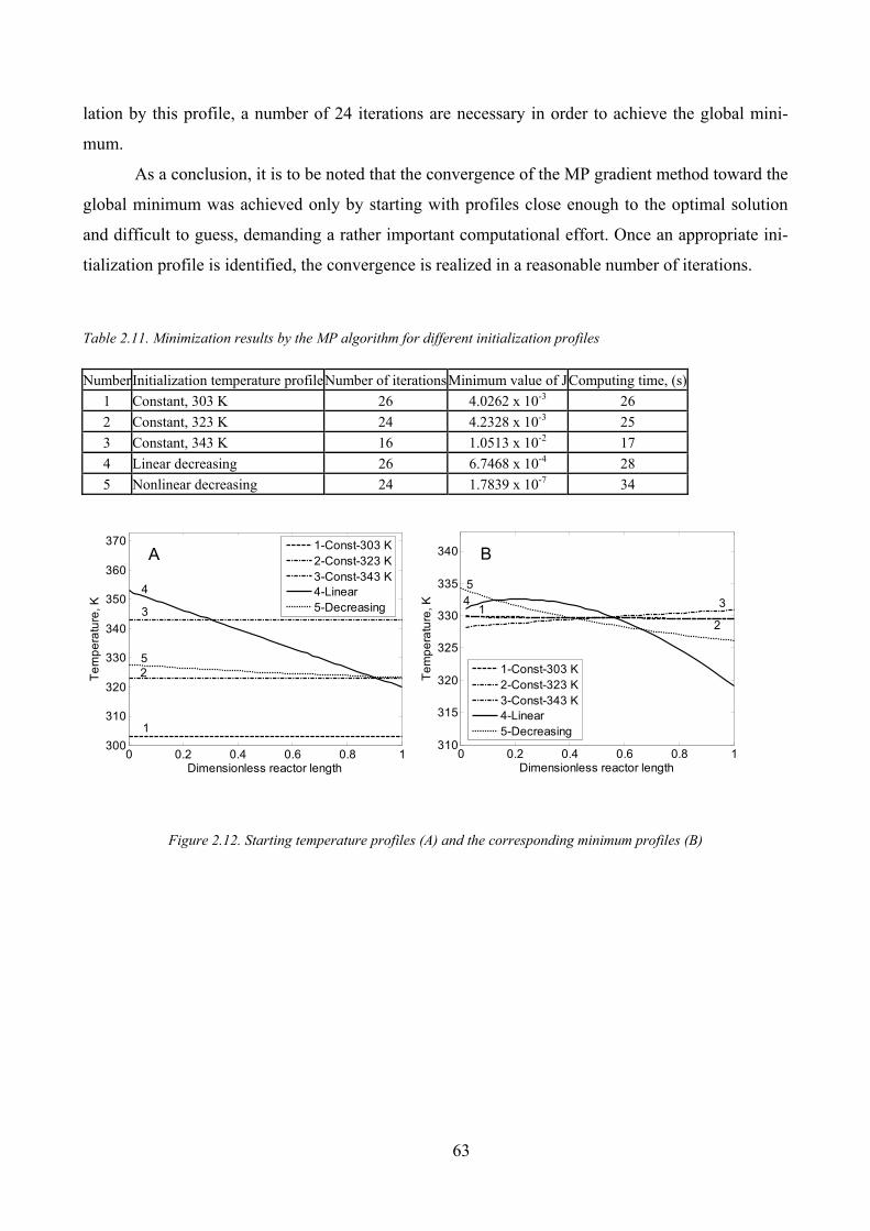
63
lation by this profile, a number of 24 iterations are necessary in order to achieve the global mini-
mum.
As a conclusion, it is to be noted that the convergence of the MP gradient method toward the
global minimum was achieved only by starting with profiles close enough to the optimal solution
and difficult to guess, demanding a rather important computational effort. Once an appropriate ini-
tialization profile is identified, the convergence is realized in a reasonable number of iterations.
Table 2.11. Minimization results by the MP algorithm for different initialization profiles
Figure 2.12. Starting temperature profiles (A) and the corresponding minimum profiles (B)
NumberInitialization temperature profile Number of iterationsMinimum value of JComputing time, (s)
1 Constant, 303 K 26 4.0262 x 10⁻³ 26
2 Constant, 323 K 24 4.2328 x 10⁻³ 25
3 Constant, 343 K 16 1.0513 x 10⁻² 17
4 Linear decreasing 26 6.7468 x 10⁻⁴ 28
5 Nonlinear decreasing 24 1.7839 x 10⁻⁷ 34
0 0.2 0.4 0.6 0.8 1300
310
320
330
340
350
360
370
Dimensionless reactor length
Te
mp
era
ture
, K
1
2
3
4
5
1-Const-303 K
2-Const-323 K
3-Const-343 K
4-Linear
5-Decreasing
A
0 0.2 0.4 0.6 0.8 1310
315
320
325
330
335
340
Dimensionless reactor length
Te
mp
era
ture
, K
1
2
34
5
1-Const-303 K
2-Const-323 K
3-Const-343 K
4-Linear
5-Decreasing
B
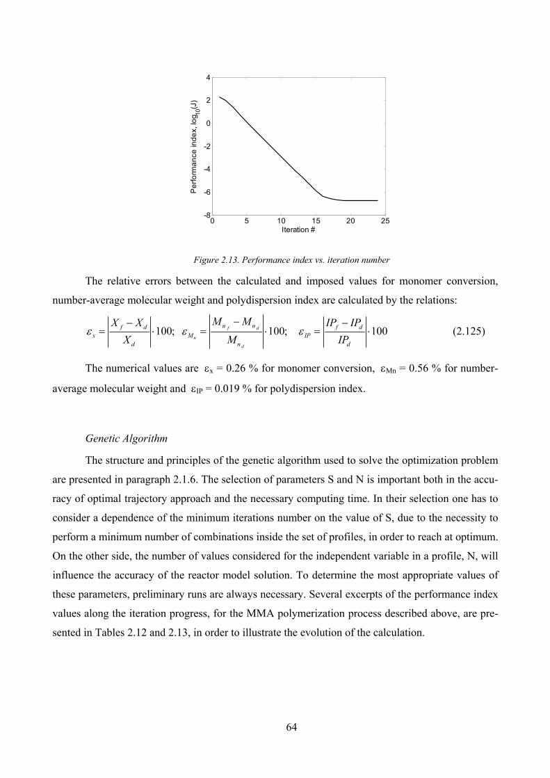
64
0 5 10 15 20 25-8
-6
-4
-2
0
2
4
Iteration #
Pe
rfo
rma
nce
ind
ex, lo
g 10(J
)
Figure 2.13. Performance index vs. iteration number
The relative errors between the calculated and imposed values for monomer conversion,
number-average molecular weight and polydispersion index are calculated by the relations:
100; 100; 100f d
n
d
n nf d f d
x M IP
d n d
M MX X IP IP
X M IPε ε ε−− −= ⋅ = ⋅ = ⋅ (2.125)
The numerical values are εx = 0.26 % for monomer conversion, εMn = 0.56 % for number-
average molecular weight and εIP = 0.019 % for polydispersion index.
Genetic Algorithm
The structure and principles of the genetic algorithm used to solve the optimization problem
are presented in paragraph 2.1.6. The selection of parameters S and N is important both in the accu-
racy of optimal trajectory approach and the necessary computing time. In their selection one has to
consider a dependence of the minimum iterations number on the value of S, due to the necessity to
perform a minimum number of combinations inside the set of profiles, in order to reach at optimum.
On the other side, the number of values considered for the independent variable in a profile, N, will
influence the accuracy of the reactor model solution. To determine the most appropriate values of
these parameters, preliminary runs are always necessary. Several excerpts of the performance index
values along the iteration progress, for the MMA polymerization process described above, are pre-
sented in Tables 2.12 and 2.13, in order to illustrate the evolution of the calculation.
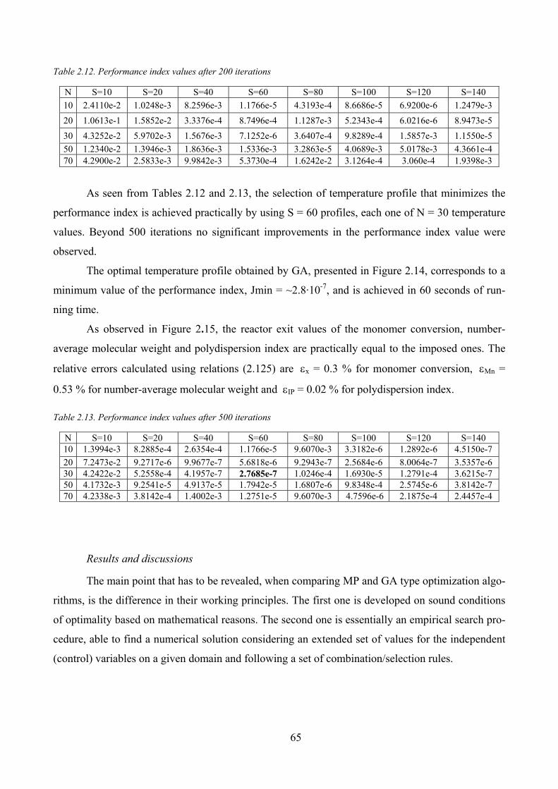
65
Table 2.12. Performance index values after 200 iterations
N S=10 S=20 S=40 S=60 S=80 S=100 S=120 S=140
10 2.4110e-2 1.0248e-3 8.2596e-3 1.1766e-5 4.3193e-4 8.6686e-5 6.9200e-6 1.2479e-3
20 1.0613e-1 1.5852e-2 3.3376e-4 8.7496e-4 1.1287e-3 5.2343e-4 6.0216e-6 8.9473e-5
30 4.3252e-2 5.9702e-3 1.5676e-3 7.1252e-6 3.6407e-4 9.8289e-4 1.5857e-3 1.1550e-5
50 1.2340e-2 1.3946e-3 1.8636e-3 1.5336e-3 3.2863e-5 4.0689e-3 5.0178e-3 4.3661e-4 70 4.2900e-2 2.5833e-3 9.9842e-3 5.3730e-4 1.6242e-2 3.1264e-4 3.060e-4 1.9398e-3
As seen from Tables 2.12 and 2.13, the selection of temperature profile that minimizes the
performance index is achieved practically by using S = 60 profiles, each one of N = 30 temperature
values. Beyond 500 iterations no significant improvements in the performance index value were
observed.
The optimal temperature profile obtained by GA, presented in Figure 2.14, corresponds to a
minimum value of the performance index, Jmin = ~2.8·10-7, and is achieved in 60 seconds of run-
ning time.
As observed in Figure 2.15, the reactor exit values of the monomer conversion, number-
average molecular weight and polydispersion index are practically equal to the imposed ones. The
relative errors calculated using relations (2.125) are εx = 0.3 % for monomer conversion, εMn =
0.53 % for number-average molecular weight and εIP = 0.02 % for polydispersion index.
Table 2.13. Performance index values after 500 iterations
N S=10 S=20 S=40 S=60 S=80 S=100 S=120 S=140 10 1.3994e-3 8.2885e-4 2.6354e-4 1.1766e-5 9.6070e-3 3.3182e-6 1.2892e-6 4.5150e-7
20 7.2473e-2 9.2717e-6 9.9677e-7 5.6818e-6 9.2943e-7 2.5684e-6 8.0064e-7 3.5357e-6 30 4.2422e-2 5.2558e-4 4.1957e-7 2.7685e-7 1.0246e-4 1.6930e-5 1.2791e-4 3.6215e-7 50 4.1732e-3 9.2541e-5 4.9137e-5 1.7942e-5 1.6807e-6 9.8348e-4 2.5745e-6 3.8142e-7 70 4.2338e-3 3.8142e-4 1.4002e-3 1.2751e-5 9.6070e-3 4.7596e-6 2.1875e-4 2.4457e-4
Results and discussions
The main point that has to be revealed, when comparing MP and GA type optimization algo-
rithms, is the difference in their working principles. The first one is developed on sound conditions
of optimality based on mathematical reasons. The second one is essentially an empirical search pro-
cedure, able to find a numerical solution considering an extended set of values for the independent
(control) variables on a given domain and following a set of combination/selection rules.
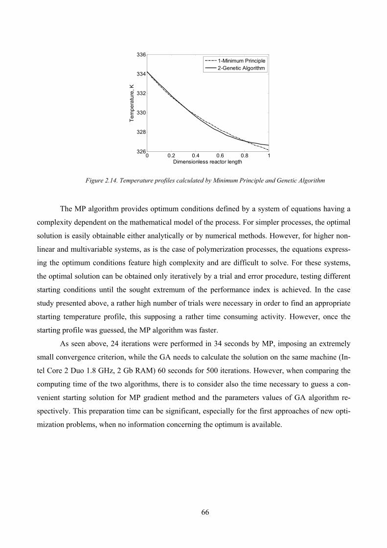
66
0 0.2 0.4 0.6 0.8 1326
328
330
332
334
336
Dimensionless reactor length
Te
mp
era
ture
, K
1-Minimum Principle
2-Genetic Algorithm
Figure 2.14. Temperature profiles calculated by Minimum Principle and Genetic Algorithm
The MP algorithm provides optimum conditions defined by a system of equations having a
complexity dependent on the mathematical model of the process. For simpler processes, the optimal
solution is easily obtainable either analytically or by numerical methods. However, for higher non-
linear and multivariable systems, as is the case of polymerization processes, the equations express-
ing the optimum conditions feature high complexity and are difficult to solve. For these systems,
the optimal solution can be obtained only iteratively by a trial and error procedure, testing different
starting conditions until the sought extremum of the performance index is achieved. In the case
study presented above, a rather high number of trials were necessary in order to find an appropriate
starting temperature profile, this supposing a rather time consuming activity. However, once the
starting profile was guessed, the MP algorithm was faster.
As seen above, 24 iterations were performed in 34 seconds by MP, imposing an extremely
small convergence criterion, while the GA needs to calculate the solution on the same machine (In-
tel Core 2 Duo 1.8 GHz, 2 Gb RAM) 60 seconds for 500 iterations. However, when comparing the
computing time of the two algorithms, there is to consider also the time necessary to guess a con-
venient starting solution for MP gradient method and the parameters values of GA algorithm re-
spectively. This preparation time can be significant, especially for the first approaches of new opti-
mization problems, when no information concerning the optimum is available.

67
Figure 2.15. Optimal state variables profiles
The GA type algorithms are more robust in the localization of optimum, due to their work-
ing principle. There is no convergence radius and, provided that the working domain and the discre-
tization of independent variables are appropriate, there is a small risk to converge towards a local
optimum. Also, these algorithms do not induce initialization difficulties, due to their internal initia-
tion mode with a family of independent variables profiles. Another important advantage of the GA
is that they are not demanding any effort in the preparation and programming of the equations giv-
ing the conditions of optimum, as in the case of MP. These features are making GA convenient op-
timization tools, especially in the case of new complex nonlinear problems. Their only disadvantage
is a rather high computing time necessary to find the optimum. However, in the conditions of the
present progresses in the digital computing, this inconvenient is becoming less and less important.
In the case of optimization problem defined above for MMA polymerization process, MP
and GA methods are giving reasonably close solutions. The minimum values of the performance
index found by the two algorithms are practically equal, with a non-significant smaller value in the
case of the MP (~1.78·10-7 comparing with ~ 2.77·10-7). The corresponding optimal temperature
0 0.2 0.4 0.6 0.8 10
0.1
0.2
0.3
0.4
0.5
0.6
0.7
Mo
no
me
r co
nve
rsio
n
Dimensionless reactor length
1-Genetic Algorithm
2-Minimum Principle
0 0.2 0.4 0.6 0.8 10
1
2
3
4
5
6
7x 10
4
Nu
mb
er
ave
rag
e m
ole
cu
lar
we
igh
t, k
g/k
mo
le
Dimensionless reactor length
1-Genetic Algorithm
2-Minimum Principle
0 0.2 0.4 0.6 0.8 11
1.5
2
2.5
Po
lyd
isp
ers
ion
in
de
x
Dimensionless reactor length
1-Genetic Algorithm
2-Minimum Principle

68
profiles comparatively presented in Figure 2.14, are practically overlapping. Also the optimal pro-
files for monomer conversion, number average molecular weight and polydispersity are graphically
presented in Figure 2.15. The final monomer conversion, number-average molecular weight and
polydispersion index calculated in optimal conditions, are practically identical with the correspond-
ing imposed values, given in Table 2.10.
To summarize, it can be asserted that the differences between the two algorithms lie in the
basic principles, complexity of the implementation and the computing times. For the case study we
considered, the two algorithms gave practically the same result, but with a significant superior effort
necessary to find an adequate starting temperature profile in the case of the gradient method based
on the MP. Once this initial profile was identified, the convergence to the optimum was attained in
a reasonable number of iterations. In the case of GA, the working principle is demanding a smaller
preparation time, but implies a much higher number of iterations in calculation and consequently, a
significant higher computing time. Supplementary runs are also necessary to optimize the values of
the algorithm parameters (number of profiles, S, number of the discretization points in a profile, N,
and the minimum number of iterations).
It is also worth to recall that the case study we considered represents an average complexity
optimization problem for a polymerization process (a single control variable, no heat balance equa-
tion necessary in the mathematical model, plug flow of reaction mixture). For more complex opti-
mization problems it could be expected supplementary difficulties in the application of MP algo-
rithms and more evident advantages in using the GA.
2.3.2. Laminar flow and plug-flow tubular reactors optimization by a
Genetic Algorithm
Optimization problem 1
Due to the strong exothermicity of the polymerization process, an appropriate control of re-
action temperature along a polymerization tubular reactor usually involves a minimum number of
cooling jackets [56]. The tubular reactors in laminar flow have pronounced temperature and compo-
sition variations across the flow direction that change the viscosity and alter the velocity profile
from the simple parabolic one. Molecular diffusion acts in the direction of diminishing the radial
gradients but will not completely eliminate them, particularly in liquid phase systems, where the
diffusivities are of the order of magnitude 10-9 to 10-10 m2 s-1 for small molecules and much lower
for the polymers [35].
69
The comparison of the simulation results for a MMA polymerization reactor in plug-flow
and laminar flow assumptions performed in paragraph 2.2 showed significant differences in calcu-
lated reaction temperature profiles in the two cases.
In this paragraph an optimization study of the laminar flow and jacketed plug-flow reactor
will be presented, based on the models described in paragraph 2.1.5. The performance index defined
by relation (2.73) and the weighting factors presented in Table 2.10 were also considered in this
problem. The Genetic Algorithm presented in paragraph 2.1.6 was adapted to solve the optimization
problem so formulated. The control variables have to obey the following restrictions:
• Temperatures: 298 373K T K< < ;
• Mass flow rate, [kg/h]: 4 0.08 10 1 10−× < < ×MD
• Initiator concentrations, [mole/L]: 4 2,05 10 5 10Ic− −× < < ×
• Solvent mass fraction in the mixture: 0.1 0.9sw< < .
The reactor characteristics are given in Table 2.9. The imposed values for monomer conver-
sion, number-average molecular weight and polydispersion index are given in Table 2.10.
The representative outlet values of temperature, monomer conversion and polymer charac-
teristics are calculated as averages of their radial profiles by using the relation (2.104).
The objective of all studies was to determine the control policies that assure at the reactor
outlet an imposed monomer conversion and specified polymer characteristics (mean molecular
weight and polydispersion index). The optimization problems consider a tubular reactor with a
jacket divided in 8 sections, each one kept at a constant temperature.
As mentioned, the selected control variables are the feed initiator concentration, the mass
flow rate, the jacket temperature profile, the feed temperature of the reaction mixture and the feed
solvent weight fraction. From practical reasons (to preclude uneconomical temperature policies in-
volving cooling of the fed reactant mixture) the feed temperature was considered equal to the tem-
perature on the first jacket section. The results of the optimization study in monomer conversion,
number-average molecular weights and polydispersion index are presented in Table 2.14 (recall
that the objective is to obtain at the reactor outlet a monomer conversion, XM,d=0.5, a mean polymer
molecular weight, Mn,d = 60000 kg/kmol and a polydispersion index, Ip,d = 2).
Optimization results for a laminar flow tubular reactor
The optimization problem was solved for two values of monomer conversion (0.5 and 0.8)
and same specified values for polymer properties (number average molecular weight, Mn=60000

70
and polydispersity index, IP=2). The results of calculations are given in Figures 2.16 – 2.22 and
Table 2.14. As seen from this table, the calculated operation policies provide values for the
monomer conversion and number-average molecular weight close to the imposed ones. A slightly
weaker performance is obtained in acheiving the specified value of polydispersion index. This result
is explained firstly by the imposed value (IP=2), a relatively difficult goal and secondly by the
strong variations of reaction rates across the flowing section, particular for the laminar flow.
Table 2.14. Optimization results for polymerization reactor in laminar flow
Optimized process performances
X, [-] Mn, [kg/kmole] IP, [-]
No Solvent mass fraction, ws, [-]
Mass flow rate,DM,0, [kg/s]
Feed initiator concentration, CI,0, [mole/L]
Calculated Imposed Calculated Imposed Calculated Imposed
1 0.810 7.391 × 10⁻³ 7.990 × 10⁻⁴ 0.502 0.5 60322 2.04 2 0.346 2.870 × 10⁻² 2.260 × 10⁻² 0.808 0.8 59931
60000 2.55
2
The results presented in Table 2.14 and Figures 2.16 and 2.17 show that the optimal opera-
tion in the case of smaller monomer conversion is demandind smaller flow rates, lower initiator
concentration, higher solvent amount in the feed and relatively higher temperatures. In this case it is
required a higher reaction temperature in order to compensate the effect of lower monomer concen-
tration on polymerization rate. By this combination of operating variables values, besides the
monomer conversion and molecular weight, it is also provided a very good control for the molecu-
lar weight distribution (smallest polydispersion index).
Corresponding to a higher amount of solvent, Figure 2.17-A shows a more flat reaction tem-
perature profiles, due to a more uniform radial velocity profile. Consequently, smaller radial varia-
tions occur for monomer conversion, number-average molecular weight and polydispersion index.
Also, a more uniform initiator and monomer consumption in radial direction is observed (Figure
2.18 -A) and, consequently, a more uniform propagation rate. This has as effect a more homogene-
ous polymer (narrower molecular weight distribution, Figure 2.20 - A).
When a higher monomer conversion (Xd=0.8) is desired, the optimization algorithm is de-
manding an operation policy with higher flow rate, higher monomer and initiator concentrations in
the feed and a lower temperature level. More pronounced radial variations of the initiator and
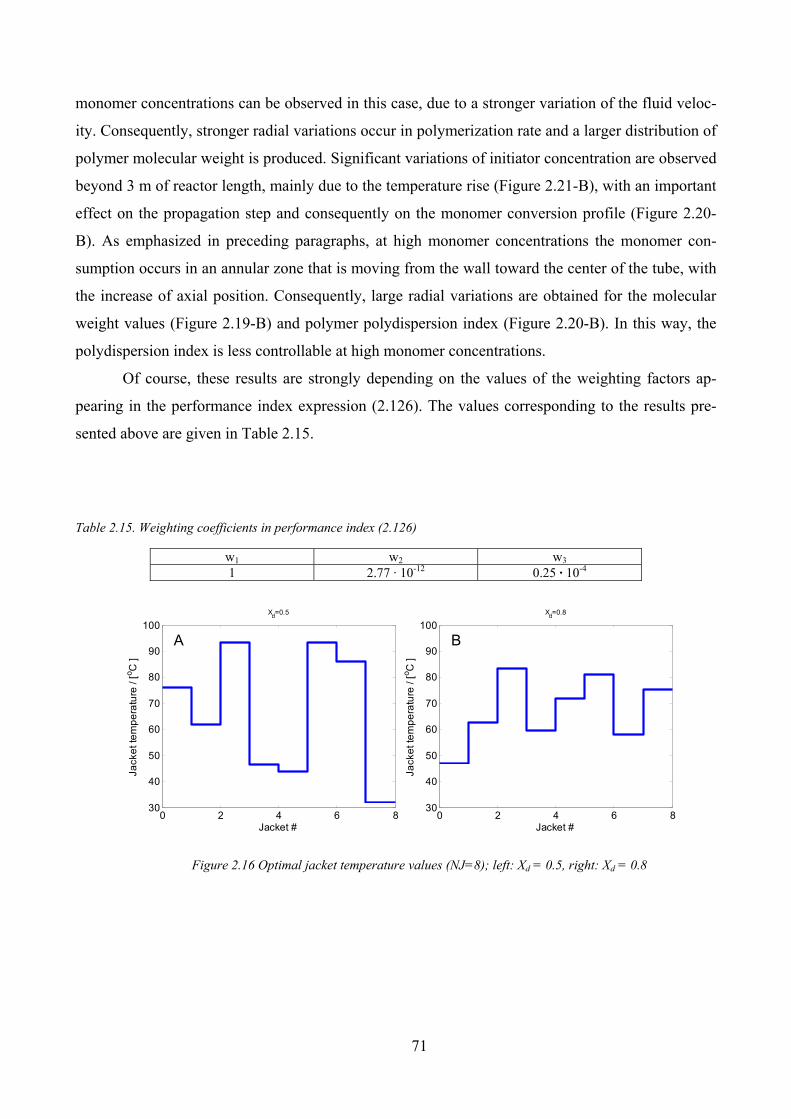
71
monomer concentrations can be observed in this case, due to a stronger variation of the fluid veloc-
ity. Consequently, stronger radial variations occur in polymerization rate and a larger distribution of
polymer molecular weight is produced. Significant variations of initiator concentration are observed
beyond 3 m of reactor length, mainly due to the temperature rise (Figure 2.21-B), with an important
effect on the propagation step and consequently on the monomer conversion profile (Figure 2.20-
B). As emphasized in preceding paragraphs, at high monomer concentrations the monomer con-
sumption occurs in an annular zone that is moving from the wall toward the center of the tube, with
the increase of axial position. Consequently, large radial variations are obtained for the molecular
weight values (Figure 2.19-B) and polymer polydispersion index (Figure 2.20-B). In this way, the
polydispersion index is less controllable at high monomer concentrations.
Of course, these results are strongly depending on the values of the weighting factors ap-
pearing in the performance index expression (2.126). The values corresponding to the results pre-
sented above are given in Table 2.15.
Table 2.15. Weighting coefficients in performance index (2.126)
w1 w2 w3
1 2.77 · 10-12 0.25 · 10-4
Figure 2.16 Optimal jacket temperature values (NJ=8); left: Xd = 0.5, right: Xd = 0.8
0 2 4 6 830
40
50
60
70
80
90
100
Jacket #
Ja
cke
t te
mp
era
ture
/ [ oC
]
Xd=0.5
0 2 4 6 830
40
50
60
70
80
90
100
Jacket #
Ja
cke
t te
mp
era
ture
/ [ oC
]
Xd=0.8
A B
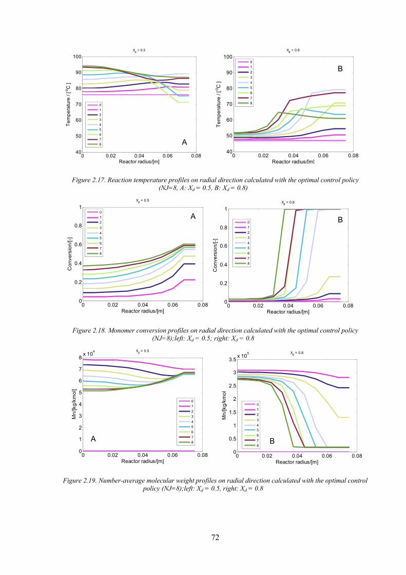
72
Figure 2.17. Reaction temperature profiles on radial direction calculated with the optimal control policy
(NJ=8, A: Xd = 0.5, B: Xd = 0.8)
Figure 2.18. Monomer conversion profiles on radial direction calculated with the optimal control policy
(NJ=8);left: Xd = 0.5; right: Xd = 0.8
Figure 2.19. Number-average molecular weight profiles on radial direction calculated with the optimal control
policy (NJ=8);left: Xd = 0.5, right: Xd = 0.8
0 0.02 0.04 0.06 0.080
0.5
1
1.5
2
2.5
3
3.5x 10
5
Reactor radius/[m]
Mn
/[kg
/km
ol
Xd = 0.8
0
1
2
3
4
5
6
7
8
0 0.02 0.04 0.06 0.080
1
2
3
4
5
6
7
8x 10
4
Reactor radius/[m]
Mn
/[kg
/km
ol]
Xd = 0.5
0
1
2
3
4
5
6
7
8 BA
0 0.02 0.04 0.06 0.080
0.2
0.4
0.6
0.8
1
Reactor radius/[m]
Co
nve
rsio
n/[-]
Xd = 0.5
0
1
2
3
4
5
6
7
8
0 0.02 0.04 0.06 0.080
0.2
0.4
0.6
0.8
1
Reactor radius/[m]
Co
nve
rsio
n/[-]
Xd = 0.8
0
1
2
3
4
5
6
7
8
A B
0 0.02 0.04 0.06 0.0840
50
60
70
80
90
100
Reactor radius/[m]
Xd = 0.5
Te
mp
era
ture
/ [ o
C ]
0
1
2
3
4
5
6
7
8
0 0.02 0.04 0.06 0.0840
50
60
70
80
90
100
Reactor radius/[m]
Te
mp
era
ture
/ [ o
C ]
Xd = 0.8
0
1
2
3
4
5
6
7
8
B
A

73
Figure 2.20. Polydispersion index profiles on radial direction calculated with the optimal control policy (NJ=8,
A: Xd = 0.5, B: Xd = 0.8)
Figure 2.21. Initiator concentration profiles on radial direction calculated with the optimal control policy
(NJ=8);left: Xd = 0.5, right: Xd = 0.8
Figure 2.22 Velocity profiles on radial direction calculated with the optimal control policy (NJ=8);left: Xd =
0.5, right: Xd = 0.8
Optimization results for a jacketed plug-flow reactor
0 0.02 0.04 0.06 0.080
0.005
0.01
0.015
0.02
Reactor radius/[m]
Ve
locity/[m
/s]
Xd = 0.8
0
1
2
3
4
5
6
7
8
0 0.02 0.04 0.06 0.080
0.2
0.4
0.6
0.8
1
1.2x 10
-3
Reactor radius/[m]
Ve
locity/[m
/s]
Xd = 0.5
0
1
2
3
4
5
6
7
8
AB
0 0.02 0.04 0.06 0.080
0.005
0.01
0.015
0.02
0.025
Reactor radius/[m]
Initia
tor
co
nce
ntr
atio
n/[m
ol/L
]
Xd = 0.8
0
1
2
3
4
5
6
7
8
0 0.02 0.04 0.06 0.080
1
2
3
4
5
6
7
8x 10
-4
Reactor radius/[m]
Initia
tor
co
nce
ntr
atio
n/[m
ol/L
]
Xd = 0.5
0
1
2
3
4
5
6
7
8
A
B
0 0.02 0.04 0.06 0.081
1.5
2
2.5
3
3.5
4
4.5
Reactor radius/[m]
Po
lyd
isp
ers
ity/[-]
Xd = 0.5
0
1
2
3
4
5
6
7
8
0 0.02 0.04 0.06 0.081
1.5
2
2.5
3
3.5
4
4.5
Reactor radius/[m]
Po
lyd
isp
ers
ity/[-]
Xd = 0.8
0
1
2
3
4
5
6
7
8
A
B
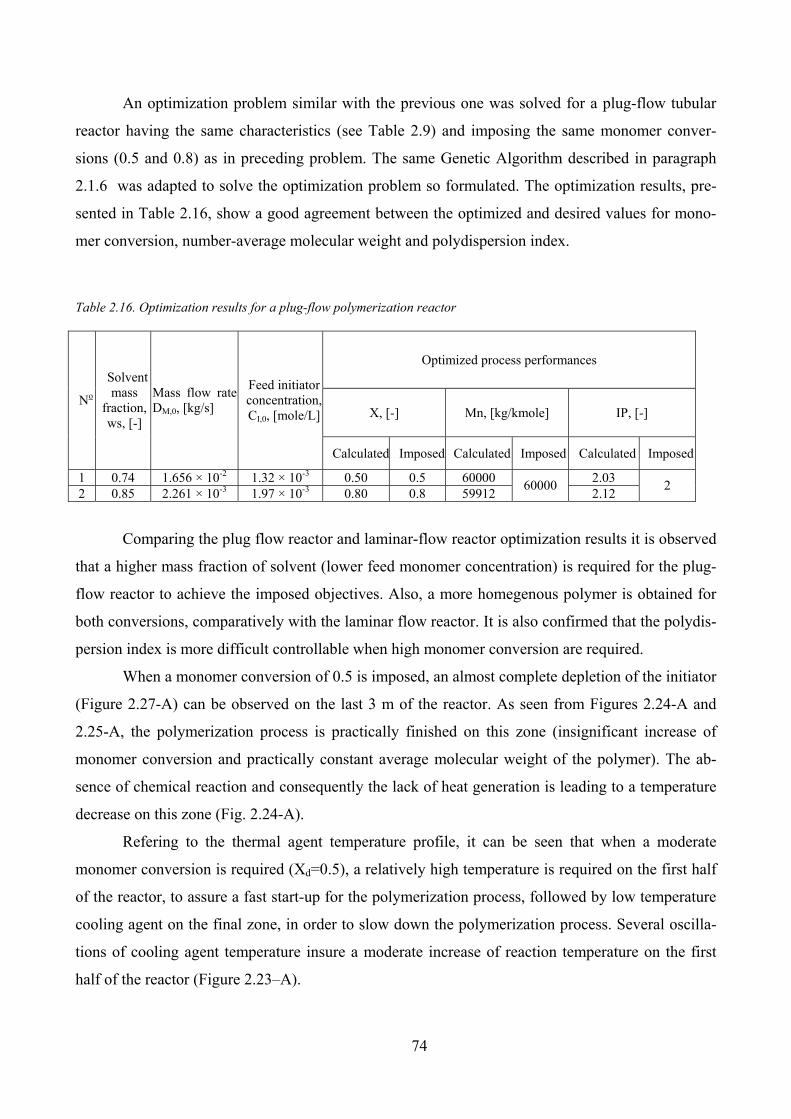
74
An optimization problem similar with the previous one was solved for a plug-flow tubular
reactor having the same characteristics (see Table 2.9) and imposing the same monomer conver-
sions (0.5 and 0.8) as in preceding problem. The same Genetic Algorithm described in paragraph
2.1.6 was adapted to solve the optimization problem so formulated. The optimization results, pre-
sented in Table 2.16, show a good agreement between the optimized and desired values for mono-
mer conversion, number-average molecular weight and polydispersion index.
Table 2.16. Optimization results for a plug-flow polymerization reactor
Comparing the plug flow reactor and laminar-flow reactor optimization results it is observed
that a higher mass fraction of solvent (lower feed monomer concentration) is required for the plug-
flow reactor to achieve the imposed objectives. Also, a more homegenous polymer is obtained for
both conversions, comparatively with the laminar flow reactor. It is also confirmed that the polydis-
persion index is more difficult controllable when high monomer conversion are required.
When a monomer conversion of 0.5 is imposed, an almost complete depletion of the initiator
(Figure 2.27-A) can be observed on the last 3 m of the reactor. As seen from Figures 2.24-A and
2.25-A, the polymerization process is practically finished on this zone (insignificant increase of
monomer conversion and practically constant average molecular weight of the polymer). The ab-
sence of chemical reaction and consequently the lack of heat generation is leading to a temperature
decrease on this zone (Fig. 2.24-A).
Refering to the thermal agent temperature profile, it can be seen that when a moderate
monomer conversion is required (Xd=0.5), a relatively high temperature is required on the first half
of the reactor, to assure a fast start-up for the polymerization process, followed by low temperature
cooling agent on the final zone, in order to slow down the polymerization process. Several oscilla-
tions of cooling agent temperature insure a moderate increase of reaction temperature on the first
half of the reactor (Figure 2.23–A).
Optimized process performances
X, [-] Mn, [kg/kmole] IP, [-] No
Solvent mass
fraction, ws, [-]
Mass flow rate,DM,0, [kg/s]
Feed initiator concentration, CI,0, [mole/L]
Calculated Imposed Calculated Imposed Calculated Imposed
1 0.74 1.656 × 10⁻² 1.32 × 10⁻³ 0.50 0.5 60000 2.03 2 0.85 2.261 × 10⁻³ 1.97 × 10⁻³ 0.80 0.8 59912
60000 2.12
2
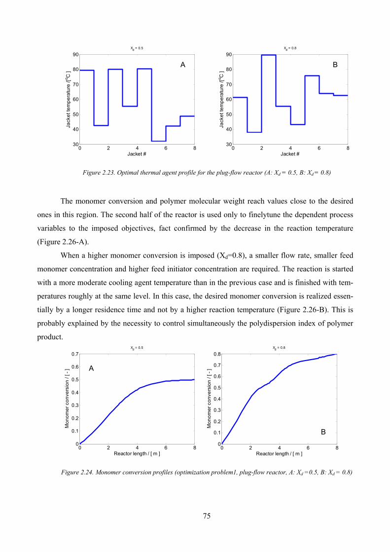
75
Figure 2.23. Optimal thermal agent profile for the plug-flow reactor (A: Xd = 0.5, B: Xd = 0.8)
The monomer conversion and polymer molecular weight reach values close to the desired
ones in this region. The second half of the reactor is used only to finelytune the dependent process
variables to the imposed objectives, fact confirmed by the decrease in the reaction temperature
(Figure 2.26-A).
When a higher monomer conversion is imposed (Xd=0.8), a smaller flow rate, smaller feed
monomer concentration and higher feed initiator concentration are required. The reaction is started
with a more moderate cooling agent temperature than in the previous case and is finished with tem-
peratures roughly at the same level. In this case, the desired monomer conversion is realized essen-
tially by a longer residence time and not by a higher reaction temperature (Figure 2.26-B). This is
probably explained by the necessity to control simultaneously the polydispersion index of polymer
product.
Figure 2.24. Monomer conversion profiles (optimization problem1, plug-flow reactor, A: Xd =0.5, B: Xd = 0.8)
0 2 4 6 80
0.1
0.2
0.3
0.4
0.5
0.6
0.7
Xd = 0.5
Reactor length / [ m ]
Mo
no
me
r co
nve
rsio
n / [ -
]
0 2 4 6 80
0.1
0.2
0.3
0.4
0.5
0.6
0.7
0.8
Xd = 0.8
Reactor length / [ m ]
Mo
no
me
r co
nve
rsio
n / [ -
]A
B
0 2 4 6 830
40
50
60
70
80
90
Jacket #
Ja
cke
t te
mp
era
ture
/[ o
C ]
Xd = 0.8
0 2 4 6 830
40
50
60
70
80
90
Jacket #
Ja
cke
t te
mp
era
ture
/[ o
C ]
Xd = 0.5
A B

76
Figure 2.25. Polymer molecular weights profiles (optimization problem1, plug-flow reactor, A: Xd =0.5, B: Xd = 0.8)
Figure 2.26.Reaction temperature profiles (optimization problem1, plug-flow reactor, A: Xd =0.5, B: Xd = 0.8)
A curious particularity of the calculated optimal regime in this case is a somewhat curious
evolution of the reaction temperature which is presenting several oscillations along the reactor (Fig-
ure 2.26-B). This is suggesting a tendency to keep the reaction temperature in close limits along the
reactor, in order to better control the polymer properties.
0 2 4 6 875
80
85
90
95
100
105
Xd = 0.5
Reactor length / [ m ]
Te
mp
era
ture
/[ o
C ]
0 2 4 6 860
62
64
66
68
70
72
74
76
Xd = 0.8
Reactor length / [ m ]
Te
mp
era
ture
/[ o
C ]
A B
0 2 4 6 80
2
4
6
8
10
12x 10
4 Xd = 0.5
Reactor length / [ m ]
Nu
mb
er-
ave
rag
e m
ole
cu
lar
we
igh
t/[ kg
/km
ol ]
0 2 4 6 80
2
4
6
8
10
12
14x 10
4 Xd = 0.8
Reactor length / [ m ]
Nu
mb
er-
ave
rag
e m
ole
cu
lar
we
igh
t/[ kg
/km
ol ]
BA
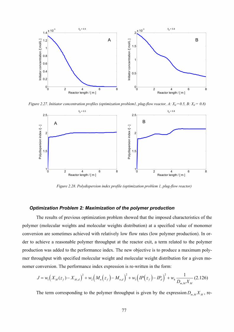
77
Figure 2.27. Initiator concentration profiles (optimization problem1, plug-flow reactor, A: Xd =0.5, B: Xd = 0.8)
Figure 2.28. Polydispersion index profile (optimization problem 1, plug-flow reactor)
Optimization Problem 2: Maximization of the polymer production
The results of previous optimization problem showed that the imposed characteristics of the
polymer (molecular weights and molecular weights distribution) at a specified value of monomer
conversion are sometimes achieved with relatively low flow rates (low polymer production). In or-
der to achieve a reasonable polymer throughput at the reactor exit, a term related to the polymer
production was added to the performance index. The new objective is to produce a maximum poly-
mer throughput with specified molecular weight and molecular weight distribution for a given mo-
nomer conversion. The performance index expression is re-written in the form:
( ) ( )( ) ( )( )2 22
1 , 2 , 3 4,
1( )M f M d n f n d f d
m M M
J w X z X w M z M w IP z IP wD X
= − + − + − + (2.126)
The term corresponding to the polymer throughput is given by the expression ,m M MD X , re-
0 2 4 6 81
1.5
2
2.5
Xd = 0.5
Reactor length / [ m ]
Po
lyd
isp
ers
ion
ind
ex /[ -
]
0 2 4 6 81
1.5
2
2.5
Xd = 0.8
Reactor length / [ m ]
Po
lyd
isp
ers
ion
in
de
x /[ -
]A B
0 2 4 6 80
0.2
0.4
0.6
0.8
1
1.2
1.4x 10
-3 Xd = 0.5
Reactor length / [ m ]
Initia
tor
co
nce
ntr
atio
n /[ m
ol/L
]
0 2 4 6 80
0.5
1
1.5
2x 10
-3 Xd = 0.8
Reactor length / [ m ]
Initia
tor
co
nce
ntr
atio
n /[ m
ol/L
] BA

78
lated to the monomer conversion and the monomer mass flow rate. The new optimization problem
was solved for the same tubular reactor, having the characteristics given in Table 2.9, for both lami-
nar flow and plug-flow hypothesis.
The values of the weighting coefficients in the performance index (2.126) given in Table
2.17 were chosen by numerical experimentation to assure the same magnitude order for each of the
terms in the considered performance index.
Table 2.17. Weighting coefficients in performance index (2.126)
Weighting coefficients w1 w2 w3 w4
1 1.4 ·10-11 2.5 · 10-5 3.0 · 10-6
Optimization of a laminar flow tubular reactor
The calculated optimal values of the solvent mass fraction, initiator concentration and mass
flow rate are presented in Table 2.18. Close values for the calculated and imposed values for mo-
nomer conversion, polymer molecular weight and molecular weight distribution were obtained. As
expected, these values are obtained with higher mass flow rates and initiator concentration, requir-
ing relatively higher thermal agent temperatures along the reactor jacket (as compared with previ-
ous optimization problem). The optimal operation policy corresponds to the cooling temperature
profile presented in Figure 2.29 and reaction temperature profiles presented in Figure 2.31 – A. This
leads to the development of polymerization process, predominantly on the second half of reactor.
Table 2.18. Results of the laminar flow tubular reactor optimization problem
On the first half of the tubular reactor only a small amount of initiator is decomposed
(Figure 2.31-B), corresponding to a low monomer conversion, due to the low level of temperature.
The small amount of primary radicals produce high molecular weights polymers (Figure 2.30 - B)
with a narrow molecular weight distribution (Figure 2.32 - A).
Due to the high monomer concentration in the feed, important radial variations of process
variables occur on the second zone of reactor length where takes place the polymerization
Optimized process performances
X, [-] Mn, [kg/kmole] IP, [-] No
Solvent mass
fraction, ws, [-]
Mass flow rate,DM,0, [kg/s]
Feed initiator concentration, CI,0, [mole/L]
Calculated Imposed Calculated Imposed Calculated Imposed
1 0.235 2.58× 10⁻¹ 4.40 × 10⁻² 0.493 0.5 60600 60000 2.19 2
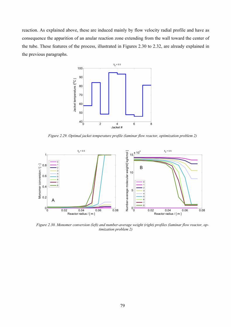
79
reaction. As explained above, these are induced mainly by flow velocity radial profile and have as
consequence the apparition of an anular reaction zone extending from the wall toward the center of
the tube. These features of the process, illustrated in Figures 2.30 to 2.32, are already explained in
the previous paragraphs.
0 2 4 6 840
50
60
70
80
90
100
Jacket #
Ja
cke
t te
mp
era
ture
/[ o
C ]
Xd = 0.5
Figure 2.29. Optimal jacket temperature profile (laminar flow reactor, optimization problem 2)
Figure 2.30. Monomer conversion (left) and number-average weight (right) profiles (laminar flow reactor, op-
timization problem 2)
0 0.02 0.04 0.06 0.080
0.2
0.4
0.6
0.8
1
Reactor radius / [ m ]
Mo
no
me
r co
nve
rsio
n / [ -
]
Xd = 0.5
0
1
2
3
4
5
6
7
8
0 0.02 0.04 0.06 0.080
5
10
15x 10
4
Reactor radius / [ m ]
Nu
mb
er-
ave
rag
e m
ole
cu
lar
we
igh
t/[ kg
/km
ol ] X
d = 0.5
0
1
2
3
4
5
6
7
8
A
B
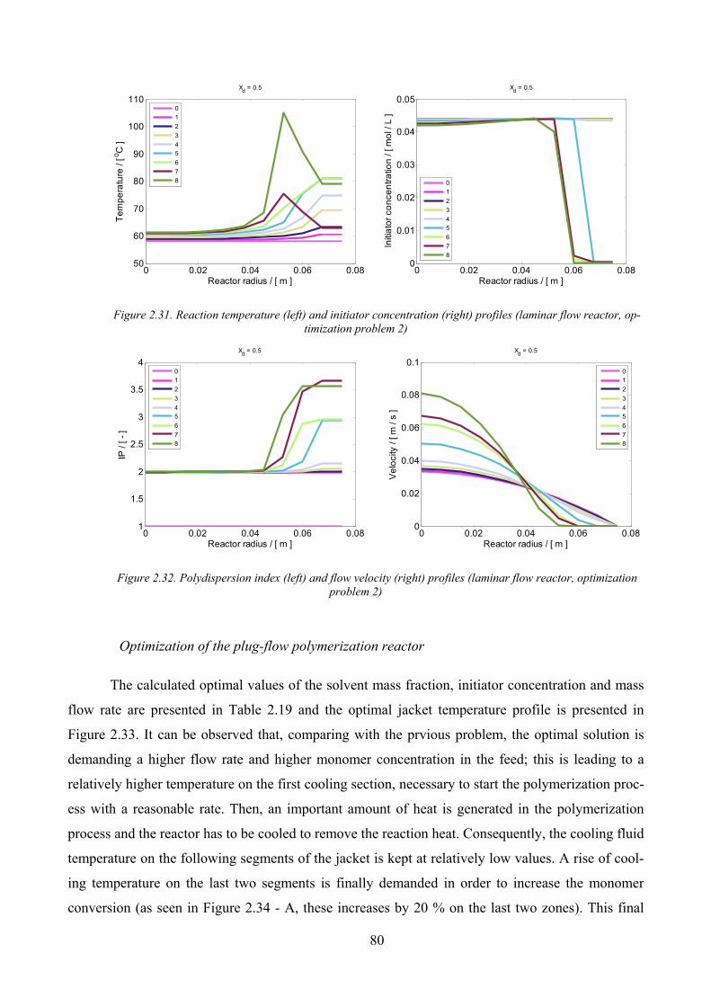
80
Figure 2.31. Reaction temperature (left) and initiator concentration (right) profiles (laminar flow reactor, op-
timization problem 2)
Figure 2.32. Polydispersion index (left) and flow velocity (right) profiles (laminar flow reactor, optimization
problem 2)
Optimization of the plug-flow polymerization reactor
The calculated optimal values of the solvent mass fraction, initiator concentration and mass
flow rate are presented in Table 2.19 and the optimal jacket temperature profile is presented in
Figure 2.33. It can be observed that, comparing with the prvious problem, the optimal solution is
demanding a higher flow rate and higher monomer concentration in the feed; this is leading to a
relatively higher temperature on the first cooling section, necessary to start the polymerization proc-
ess with a reasonable rate. Then, an important amount of heat is generated in the polymerization
process and the reactor has to be cooled to remove the reaction heat. Consequently, the cooling fluid
temperature on the following segments of the jacket is kept at relatively low values. A rise of cool-
ing temperature on the last two segments is finally demanded in order to increase the monomer
conversion (as seen in Figure 2.34 - A, these increases by 20 % on the last two zones). This final
0 0.02 0.04 0.06 0.081
1.5
2
2.5
3
3.5
4
Reactor radius / [ m ]
IP / [ -
]
Xd = 0.5
0
1
2
3
4
5
6
7
8
0 0.02 0.04 0.06 0.080
0.02
0.04
0.06
0.08
0.1
Reactor radius / [ m ]
Ve
locity
/ [ m
/ s
]
Xd = 0.5
0
1
2
3
4
5
6
7
8
0 0.02 0.04 0.06 0.0850
60
70
80
90
100
110
Reactor radius / [ m ]
Te
mp
era
ture
/ [ o
C ]
Xd = 0.5
0
1
2
3
4
5
6
7
8
0 0.02 0.04 0.06 0.080
0.01
0.02
0.03
0.04
0.05
Reactor radius / [ m ]
Initia
tor
co
nce
ntr
atio
n / [ m
ol /
L ]
Xd = 0.5
0
1
2
3
4
5
6
7
8

81
temperature evolution is perturbing the polydispersion index, which is displacing away from the
desired value, on the last two reactor zones (Figure 2.36).
A value for polydispersion index closer to the desired one could be achieved by increasing
the weighting factor w3, but with sacrifices in the approaching of desired values in number-average
molecular weight and monomer conversion.
Table 2.19. Results of the plug-flow reactor optimization problem 2
0 2 4 6 820
30
40
50
60
70
80
90
Jacket #
Ja
cke
t te
mp
era
ture
/[ o
C ]
Xd = 0.5
Figure 2.33. Optimal jacket temperature profile (plug-flow reactor, optimization problem 2)
Figure 2.34. Monomer conversion (left) and number-average weight (right) profiles (plug-flow reactor, optimization
problem 2)
Optimized process performances
X, [-] Mn, [kg/kmole] IP, [-] No
Solvent mass
fraction, ws, [-]
Mass flow rate,DM,0, [kg/s]
Feed initiator concentration, CI,0, [mole/L]
Calculated Imposed Calculated Imposed Calculated Imposed
1 0.57 4.24× 10⁻² 2.31 × 10⁻³ 0.499 0.5 60007 60000 2.29 2
0 2 4 6 80
0.1
0.2
0.3
0.4
0.5
Xd = 0.5
Reactor length / [ m ]
Mo
no
me
r co
nve
rsio
n / [ -
]
0 2 4 6 80
0.5
1
1.5
2x 10
5 Xd = 0.5
Reactor length / [ m ]
Nu
mb
er-
ave
rag
e m
ole
cu
lar
we
igh
t/[ kg
/km
ol ]
A B

82
Figure 2.35. Reaction temperature (left) and initiator concentration (right) profiles (plug-flow reactor, optimi-
zation problem 2)
0 2 4 6 81
1.5
2
2.5
Xd = 0.5
Reactor length / [ m ]
Po
lyd
isp
ers
ion
ind
ex /[ -
]
Figure 2.36. Polydispersion index profile (plug-flow reactor, optimization problem 2)
2.4. Conclusions
The objectives of this chapter was to investigate the particularities of modeling and optimi-
zation problems for tubular polymerization reactors and to compare the performance of two optimi-
zation methods, one based on Minimum Principle of Pontryagin and the other on a Genetic Algo-
rithm. As a case study it was chosen the MMA solution polymerization process due to the availabil-
ity of the kinetic data. Two types of tubular reactor models were developed, one in plug-flow as-
sumptions and the other a bi-dimensional laminar flow, taking into account the radial variation of
the flow velocity. The most representative among the published kinetic models was chosen by reac-
tor simulations, comparing the agreement of the results in terms of simulated monomer conversion
and number-average molecular weight. The model of Baillagou and Soong (1985) appeared from
these stand point as the most representative.
Calculation procedures for the plug-flow and laminar flow regimes were developed and used
in the polymerization reactor simulation. A comparison of reactor performances for the two flow
0 2 4 6 870
80
90
100
110
120
Xd = 0.5
Reactor length / [ m ]
Te
mp
era
ture
/[ o
C ]
0 2 4 6 80
0.5
1
1.5
2
2.5x 10
-3 Xd = 0.5
Reactor length / [ m ]
Initia
tor
co
nce
ntr
atio
n /[ m
ol/L
]
A B
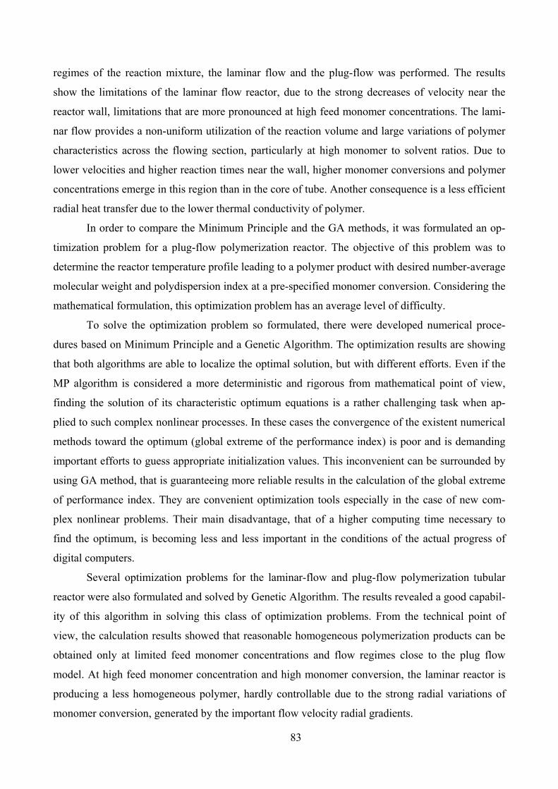
83
regimes of the reaction mixture, the laminar flow and the plug-flow was performed. The results
show the limitations of the laminar flow reactor, due to the strong decreases of velocity near the
reactor wall, limitations that are more pronounced at high feed monomer concentrations. The lami-
nar flow provides a non-uniform utilization of the reaction volume and large variations of polymer
characteristics across the flowing section, particularly at high monomer to solvent ratios. Due to
lower velocities and higher reaction times near the wall, higher monomer conversions and polymer
concentrations emerge in this region than in the core of tube. Another consequence is a less efficient
radial heat transfer due to the lower thermal conductivity of polymer.
In order to compare the Minimum Principle and the GA methods, it was formulated an op-
timization problem for a plug-flow polymerization reactor. The objective of this problem was to
determine the reactor temperature profile leading to a polymer product with desired number-average
molecular weight and polydispersion index at a pre-specified monomer conversion. Considering the
mathematical formulation, this optimization problem has an average level of difficulty.
To solve the optimization problem so formulated, there were developed numerical proce-
dures based on Minimum Principle and a Genetic Algorithm. The optimization results are showing
that both algorithms are able to localize the optimal solution, but with different efforts. Even if the
MP algorithm is considered a more deterministic and rigorous from mathematical point of view,
finding the solution of its characteristic optimum equations is a rather challenging task when ap-
plied to such complex nonlinear processes. In these cases the convergence of the existent numerical
methods toward the optimum (global extreme of the performance index) is poor and is demanding
important efforts to guess appropriate initialization values. This inconvenient can be surrounded by
using GA method, that is guaranteeing more reliable results in the calculation of the global extreme
of performance index. They are convenient optimization tools especially in the case of new com-
plex nonlinear problems. Their main disadvantage, that of a higher computing time necessary to
find the optimum, is becoming less and less important in the conditions of the actual progress of
digital computers.
Several optimization problems for the laminar-flow and plug-flow polymerization tubular
reactor were also formulated and solved by Genetic Algorithm. The results revealed a good capabil-
ity of this algorithm in solving this class of optimization problems. From the technical point of
view, the calculation results showed that reasonable homogeneous polymerization products can be
obtained only at limited feed monomer concentrations and flow regimes close to the plug flow
model. At high feed monomer concentration and high monomer conversion, the laminar reactor is
producing a less homogeneous polymer, hardly controllable due to the strong radial variations of
monomer conversion, generated by the important flow velocity radial gradients.

84
85
3. Modeling and optimization of the PLA synthesis process
by reactive extrusion

86
3.1. Literature survey
The world-wide production of consumer plastics continues to be dominated by petroleum-
based polymers. The biodegradable polymers have been made economically attractive by two fac-
tors: the first, the environmental concern associated with waste disposal and the second, the future
depletion of the most accessible petroleum reserves and consequently rising of the production costs.
Polylactide (PLA) belongs to the family of synthetic aliphatic polyesters and is considered
as biodegradable and compostable. It is a thermoplastic, high strength, high modulus polymer that
can be obtained from annually renewable resources [57]. The degradability, versatility and antici-
pated price/performance of the new generation of polymers, PLA, will enable it to displace a sig-
nificant volume of fossil fuel-based polymers.
Historical survey and PLA practical applications
Many investigations were performed along the last century on the lactic acid polymers. In
1985, Pelouze condensed lactic acid by distillation of water to form low molecular weight PLA, and
the lactide (cyclic dimer of lactic acid) [58]. The polymer was produced for the first time in 1932 by
Carothers (DuPont), heating lactic acid under vacuum to produce a low molecular weight product
[59]. Although the polymer was known since the specified period, it was not of practical usefulness
until recently. In 1988, Cargill Incorporated began the investigation of lactide and PLA and con-
cluded that PLA is an interesting material. After years of research, Cargill managed to manufacture
PLA in 1994, with 4000 t/year capacity. It was produced in a fully commercial manufacture by
Cargill Dow in November 2001 [58]. In 2002, the PLA manufacture in the US federal state Ne-
braska had an production of 140 000 t/year PLA [60].
Nowadays, several companies in USA, Japan and Germany are currently creating modern
technologies for production of lactic acid, polylactides and polymeric materials based on these raw
materials. The basic manufacturers of these materials are: Cargill Dow Polymers (polymer and fi-
bres NatureWorks™), Kanebo Goshen Ltd. (polymer and fibres Lactron™), Shimadzu Corp (Lac-
tyl®), Ems Inventa Fischer GmbH & Co [61].
Subsequent work by DuPont and Ethicon has focused on the manufacture of PLA for medi-
cal-grade sutures, implants and controlled drug release applications. Shimadzu and Mitsui Tuatsu
companies in Japan produce also limited quantities of PLA for “commodity” plastics applications.
The advances in the fermentation of dextrose obtained from corn has dramatically reduced the cost
87
to manufacture the lactic acid monomer necessary to make PLA polymers [59].
Polylactide is used mainly for medical applications, but recently it is accepted also to play a
major role as a packaging material. Numerous studies indicate that the polylactides are sufficiently
biocompatible, with a minority suggesting otherwise [62-64]. The precise molecular structure de-
termines their rate of degradation and since the degradation products are natural and metabolizable
the process is generally well accepted [4]. It is stated in the published literature that the degradation
time of L-PLA is much slower than that of DL-PLA requiring more than 2 years to be completely
absorbed. A solution was to prepare copolymers of L-lactide with glycolide or DL-lactide in order
to disrupt L-lactide crystallinity accelerating the degradation process [62].
PLA materials can be produced with a large range of properties, due to the nature of lactic
acid, a chiral molecule with two asymmetric centers existing in four different forms. The molecular
weights of PLA can vary from few thousands to over a million. Also, it can be easily converted into
film, fiber, spun bond and melt blown products on existing processing equipment [59].
The rheological characteristics of PLA make it well suited for sheet extrusion, film blowing,
and fiber spinning, but only marginally acceptable for some other types of fabrication [65]. The
properties and temperature characteristics of polylactide are comparatively close to polypropylene and
polycaproamide. The fiber and filament fabrication processes and equipment used are also similar. The usual
production process includes spinning, thermal drawing, heat treatment (thermal relaxation), and final textile
operations which are a function of the commercial forms and assortment of fibers and/or filaments. This is
an almost no-waste process, since all wastes formed are recycled [61].
Monomers and polymerization processes
The basic constitutional unit of PLA, the lactic acid was first isolated in 1780 from sour milk
by the Swedish chemist Scheele and produced commercially in 1881 [66]. It can be manufactured
by carbohydrates fermentation or chemical synthesis [64, 67]. It is the simplest hydroxyl acid with
an asymmetric carbon atom and it exist in two optically active configurations, the L(-) and D(+)
isomers [68]. L-lactic acid is present in mammals while both stereoisomers are found in bacteria
[57]. Nowadays, the majority of the fermentation processes use a genus of Lactobacilli which yields
a high rate of lactic acid. Moreover, a recent study developed a process to produce mainly L-lactic
acid including incubating acid-tolerant homolactic bacteria in nutrient medium [67]. It was found
that hetero-fermentative lacto-bacteria produce a racemic mixture of D and L-lactic acid [60].
The conversion of lactic acid into PLA can be carried out following two routes. The first
route involves the direct polycondensation reaction and removal of water product under high vac-
88
uum and high temperature [1, 10, 14], while vacuum and temperature are progressively increased
[59]. The polycondensation could be seen as the easiest route, but it is difficult to reach high mo-
lecular weights through a solvent-free process [57]. Addition of acidic catalysts, such as boric or
sulfuric acid accelerates the esterification and transesterification processes, but also catalyzes side
reactions. Also the low molecular weights condensates could be of practical interest in preparation
of biodegradable glues and lacquers because the -OH and -COOH end groups allow cross-linking
with suitable inorganic or organic multivalent additives [59]. The properties of lactic acid oli-
gomers, which can be further used to synthesize polyurethanes, can be controlled using different
operating conditions and the type of catalyst and functional agents [69]. This approach was used by
Carothers and it is still used by Mitsui Toatsu Chemicals Inc. to produce a low molecular weight
polymer [59].
An alternative of PLA producing from lactic acid is the ring-opening polymerization of lac-
tic acid dimmer, di-lactide. Water is removed under mild conditions, without a solvent, to produce
the cyclic dimmer from lactic acid. A process in which lactide is purified by an improved distilla-
tion system with the substantially purified lactide removed as an intermediate boiling side-draw
stream was proposed in the published literature [70]. Other efficient processes were proposed to
transform lactic acid into its cyclic dimmer [16-18]. The process was industrially applied by Cargill
Dow [70-74]. Function of lactide purity can be obtained a large range of molecular weight polymers
[59].
L-lactide ring-opening polymerization. Polymerization initiators and mechanisms
Considerable experimental work was done by various investigators to study the reaction ki-
netics of ring-opening polymerization. In experimental studies, various catalyst systems, solvents
and reaction temperature have been used to obtain polymers of molecular weights ranging from a
few thousands to over a million.
The lactide polymerization initiators could be divided into three cathegories:
• Lewis acids, Sn(Ph)4, SnBr4, stannous octoate - SnOct2, zinc acetate - ZnAc2, Sb2O5, zinc
lactate - ZnLac2 . They promote the polymerization by compounds containing hydroxyl groups
following the coordination-insertion mechanism. There are commercially available, easy to
handle, soluble in common organic solvents. Some of them are potentially non-toxic.
• Metal-alkoxides: Al(OR)3, R3SnOR’, Ti(OR)4, which are supposed to be the true initiators of
ring-opening polymerization of L-lactide. However they have increased toxicity, for example
aluminium tri-isopropoxyde, Al(O-iPr)3 is suspected of supporting Alzeimer’s disease [75];
89
• Other initiators as N-carbenes, racemic catalyst, calcium and magnesium complexes, enzymes
having the advantage of biocompatibility and low-toxicity. The main disadvantage of this third
category of initiators is the impossibility to know exactly the kinetic mechanism.
Recent studies include dimeric aluminum chloride complexes of N-alkoxyalkyl- く-
ketoimines (activation with propylene oxide), alkoxy-amino-bis (phenolate) Group 3 metal com-
plexes [76], aluminum complexes bearing tetradentate bis(aminophenoxide) ligands, hetero-
bimetallic iron(II) alkoxide/aryloxides, stannous octoate and diethanolamine, く –diiminate ligated
magnesium and zinc complexes [77], zinc alkoxide complex, magnesium and zink alkoxides [78],
titanium alkozide, iron alkoxide [79, 80], 2,6- dimethyl aryloxide, calcium coordination complexes
[81], complexes of Cu, Zn, Co and Ni Schiff base derived from salicylidene and L-aspartic acid,
dizinc-monoalkoxide complex supported by a dinucleating ligand, stannous octoate with adducts
containing oligomers L-lactide and rac-lactide [82], tertiary amines, phosphines and N-heterocyclic
carbenes, alkyl aluminum, aluminum – achiral ligands complexes and lithium chloride [83, 84].
Polymerization studies involving fully biocompatible initiators (creatinine) for L-lactide ring-
opening polymerization were published but only low molecular weights polymers were produced
[85].
The published works in the field of L-lactide polymerization were reviewed by Stridsberg et
al [86], Drumright et al [65], Wu et al [87] and Dechy-Cabaret et al [75].
The published studies showed an increased effect in development of an efficient and simple
kinetic mechanism for L-lactide polymerization. It was demonstrated that lactones polymerization
using aluminium and tin alkoxides proceeds via an insertion mechanism [88]. Dubois et al hypothe-
sized that the L-lactide ring-opening polymerization initiated by aluminium alkoxide proceeds
through a “coordination-insertion” mechanism and selective rupture of the acyl-oxygen bond of the
monomer [89-91].
The most used initiator for the L-lactide polymerization process is SnOct2, its advantages
being the high catalytic activity, racemization-free polymerization of L-lactide, formation of high-
molecular weight polymers with high yields and its acceptance by the US Food and Drug Admini-
stration, etc [92, 93]. Usually a primary alcohol is used as co-initiator, which fulfills three purposes:
it accelerates the polymerization process, allows a control for molecular weights and does form es-
ter end-groups which can be used for further preparative or analytical purposes (1H NMR determi-
nation of the degree of polymerization) [94].
One of the first studies concerning L-lactide polymerization using stannous octoate as initia-
tor was published in 1987 by Eenink [95] . The study reports data concerning the influence of proc-

90
ess parameters on the polymer characteristics. Other work reporting the influence of monomer pu-
rity on the polymer molecular weights for L-lactide/stannous octoate polymerization system was
published by Lian-Xi et al [96].
Nijenhuis et al studied the kinetics and mechanism of L-lactide bulk polymerization using
stannous octoate and zinc bis (2,2 – dimethyl –3,5 – heptanedionate – O, O’). The monomer conver-
sions up to 80 % conversion were obtained and the rate of polymerization using tin compound was
higher than that with zinc-containing initiator, while at conversions beyond 80%, the latter initiator
gave the higher rate of polymerization. The differences in the rate of polymerization at high conver-
sions for the two catalysts are suggested to be caused by a difference in crystallinity of the newly
formed polymer. It is suggested that contaminants in the catalyst and the monomer are the true ini-
tiators. Initiation as well as polymerization is supposed to proceed through Lewis acid catalyzed
transesterification between an activated lactone and a hydroxyl group [97].
Methyltriflat [98] and stannous(II) trifluormethane sulphonate [99] were mentioned as cati-
onic initiators for L-lactide polymerization in the published literature. Few studies have speculated
about a cationic mechanism [100, 101] for stannous octoate initiated L-lactide polymerization.
Schwach et al [101] studied the ring opening polymerization of PLA in the presence of SnOct2 un-
der conditions allowing for the end – group characterization of growing chains by high-resolution 1H-NMR.
For low values of monomer to initiator ratios, the D, L-Lactide ring was opened to yield lac-
tyl octoate-terminated short chains. A cationic type mechanism (Figure 3.1) involving coordination
by octanoic acid was proposed to account for experimental findings.
Kricheldorf et al performed the anionic L-lactide polymerization in solution was performed
using potassium benzoate, potassium phenoxide, potassium tert-butoxide and butyllitium as initia-
tors. Absence of initiator fragments in the isolated PLA chains suggested that initiator mainly in-
volve deprotonation of L-lactide. It was also proved that the alkoxide chain end cause partial race-
mization [102].
The effect of Lewis bases co-initiators in the polymerization of L-lactide using SnOct2 as in-
itiator is studied by Degée et al [92]. The monomer was dried under reduced pressure before use
and the initiator was purified by two vacuum distillations. The authors didn’t discover any direct
relationship between molecular weight and the maximum conversion. The polymerization rate de-
creases as the monomer/initiator ratio (M/I) is increased.
Degée et al revealed that M/I values lower than 1000, the number-average molecular weight
values are higher than those expected on the basis of the initial monomer to catalyst initial ratio
(assuming quantitative initiation) and they supposed that stannous octoate is not the actual initiator.
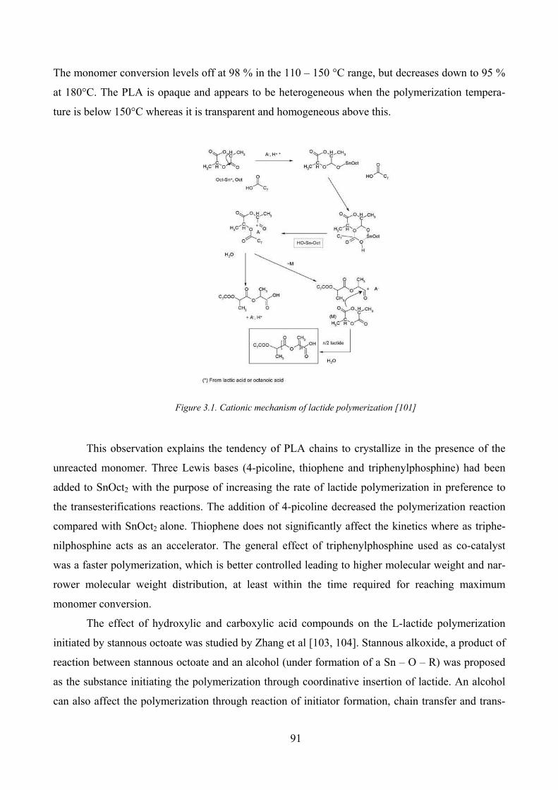
91
The monomer conversion levels off at 98 % in the 110 – 150 °C range, but decreases down to 95 %
at 180°C. The PLA is opaque and appears to be heterogeneous when the polymerization tempera-
ture is below 150°C whereas it is transparent and homogeneous above this.
Figure 3.1. Cationic mechanism of lactide polymerization [101]
This observation explains the tendency of PLA chains to crystallize in the presence of the
unreacted monomer. Three Lewis bases (4-picoline, thiophene and triphenylphosphine) had been
added to SnOct2 with the purpose of increasing the rate of lactide polymerization in preference to
the transesterifications reactions. The addition of 4-picoline decreased the polymerization reaction
compared with SnOct2 alone. Thiophene does not significantly affect the kinetics where as triphe-
nilphosphine acts as an accelerator. The general effect of triphenylphosphine used as co-catalyst
was a faster polymerization, which is better controlled leading to higher molecular weight and nar-
rower molecular weight distribution, at least within the time required for reaching maximum
monomer conversion.
The effect of hydroxylic and carboxylic acid compounds on the L-lactide polymerization
initiated by stannous octoate was studied by Zhang et al [103, 104]. Stannous alkoxide, a product of
reaction between stannous octoate and an alcohol (under formation of a Sn – O – R) was proposed
as the substance initiating the polymerization through coordinative insertion of lactide. An alcohol
can also affect the polymerization through reaction of initiator formation, chain transfer and trans-
92
esterification. Zhang et al showed that the alcohol increases the PLA production rate while carbox-
ylic acids decrease it. Both alcohol and carboxylic acids was found to reduce the PLA final molecu-
lar weights.
Kricheldorf [94, 105] studied model reactions between pure SnOct2 and primary alcohols.
Both L-lactide and stannous octoate were purified before using. The authors reveal the fact that a
rapid equilibrium between SnOct2 and benzylalcohol occurs even at 20°C and the formation of a
SnOct2 – alcohol complex was formulated. An increasing downfield shift of the OH – proton was
observed with higher SnOct2/alcohol ratios. The continuation of this study using 13C NMR spec-
troscopy has revealed that the CO – signal of SnOct2 shifts upfield in direction of the value typical
for the free octanoic acid when an alcohol is added. The NMR spectroscopy results revealed a rapid
equilibrium between the octoate groups of Sn(Oct)2 and the added alcohol leading to octanoic acid
molecules.
Kowalski et al [106-108] revealed that the actual active centers can be formed with adventi-
tious water, hydroxyl acids and some others unknown co-initiators present as impurities in the po-
lymerization mixture. With water as impurity, the following interchange reactions take place:
2SnOct HOH OctSnOH OctH⎯⎯→+ +←⎯⎯ (3.1)
( )2OctSnOH HOH Sn OH OctH⎯⎯→+ +←⎯⎯ (3.2)
with subsequent propagation by monomer insertion into the –Sn-OH bonds:
( )n
OctSnOH nM Oct Sn O m H+ ⎯⎯→ − − − − (3.3)
where Oct denotes the 2-ethyl hexanoate group and m the polyester repeating unit derived
from M.
Addition of 2-ethylhexanoic acid to the system was found to decrease the rate of polymeri-
zation and practically does not influence the number-average molecular weights. The rates decrease
because growing chains are converted into the dormant ones by displacing the alkoxide active chain
from tin atom. The higher the concentration of the added acid the lower the instantaneous concen-
tration of growing chains::
( ) ( )2n n
OctSnO m H OctH SnOct HO m OH
active species inactive species
− − + ⎯⎯→ + − − (3.4)
To speed up the polymerization reaction, the acids present in the polymerization mixture
should be removed. Storey and Taylor [109] reported NMR data showing that SnOct2 reacts directly
with hydroxyl groups giving eventually the respective 2-ethylhexanoate ester.
Esterification may also proceed with the already formed hydroxy-PLA, e.g.:
93
2( )' '2( ) ( ) ( ) ( )⎯⎯⎯⎯→+ − − − − +←⎯⎯⎯⎯Sn Oct
n nRC O OH HO m R RC O m R H O (3.5)
The presence of Sn atoms in macromolecules is the argument for polymerization proceeding
with Sn – alkoxides as an active species.
Kowalski et al [4] published a comparison between polymerization of L-lactide initiated by
SnOct2 with and without adding a co-initiator. In the case of polymerization reaction using as initia-
tor SnOct2 alone, the dependence of relative polymerization rate in respect with initial concentration
of stannous octoate was studied. At lower initiator concentrations the rate increases almost linearly
with starting initiator concentration until a critical value is reached; then further increase of polym-
erization rate is less steep, and after reaching a maximum, it eventually decreases with further in-
creasing initiator concentration. The result means that the adventitious co-initiator does exist in both
solvent/monomer mixture and in SnOct2 itself. Thus, above a certain initiator concentration any
further increase in rate is only due to the co-initiator present in SnOct2. A slight retarding effect is
probably caused either by the octanoic acid introduced as an impurity with SnOct2. The system used
for polymerization contained approximately 10-3 mol/L of adventitious hydroxyl compounds as co-
initiator.
When using as initiating system a mixture of stannous octoate and butanol (BuOH) at a con-
stant concentration of SnOct2, at lower starting concentrations of butanol, the polymerization rate
increases proportionally to butanol initial concentration (BuOH0). When a certain ratio
BuOH/SnOct2 is reached, the rate becomes independent of BuOH0. Moreover, with increasing
BuOH0 , molar weights decrease. In this case, it was revealed that the alcohol plays a double role, of
co-initiator and of transfer agent. The same role could be played by any hydroxyl compound present
in the polymerization mixture, as follows:
• formation of an initiator
2( )Sn Oct ROH OctSnOR OctH⎯⎯→+ +←⎯⎯ (3.6)
• reversible chain transfer
( ) ( )n nOctSnO m OR ROH OctSnOR HO m R⎯⎯→− − + + − −←⎯⎯ (3.7)
The reaction (3.7) decreases the total concentration of macromolecules able to grow (active
or dormant) by forming the dead molecules ( )( )nOct m R− − . Some new initiating species may be
formed in the reaction of the esterification byproduct, H2O, following the reactions (3.1) and (3.2)
respectively. These reactions increase the number of the growing species, increasing polymerization
rate this way. In parallel reactions, carboxylic acid is formed and inhibits polymerization.
Esterification and formation of octanoic ester end groups are much less important in L-
94
lactide polymerization than in the polymerization of caprolactone. Concentration of the esterified
macromolecules at the final equilibrium would presumably be close to double the initial stannous
octoate concentration.
Polymerization with an initial concentration of stannous octoate of 0.05 mol/L with no alco-
hol added was proved to be very slow by Kowalski et al because it is certainly initiated by com-
pounds containing hydroxyl groups, adventitiously present in the system as impurities. The authors
assumed that one molecule of co-initiator give rise to one macromolecule, the concentration of the
co-initiator calculated from 5 11.5 10 ·nM mol L−= × of the resulting polymer, was equal to
3 110 ·mol L− −≈ . Polymerization initiated with stannous butoxide in concentration of 0.05 mol/L was
22.4·10 times faster than with only SnOct2 alone.
The rate of polymerization in the system with octanoic acid added to stannous butoxide was
approximately 2 times lower. That support the hypothesis that approximately 90 % mol of stannous
alkoxide became temporarily deactivated.
Kricheldorf et al [94, 105] has shown that both anionic and cationic polymerization of L-
lactide involve strong racemization above 50°C, whereas SnOct2 yields optically pure PLA even at
180 °C, when the reaction time is short. The SnOct2 used in experiments was dried firstly by twice
distillation with xylene under reduced pressure and finally subjected to a fractionated distillation in
vacuum. The L-lactide from Boehringer KG (Ingelheim, Germany) was recrystallized from ethyl
acetate.
The authors polymerized the L-lactide at 180°C with neat SnOct2 under variation of M/I ra-
tio. The molecular weight were dependent on the M/I ratio and all the samples contained significant
amounts of octoate end groups. The values of degree of polymerization indicated that, on the aver-
age, only one octoate group per initiator was transformed into an end group. The highest monomer
conversion was obtained at 180°C, using a M/I ratio of 200 and a reaction time of one hour.
Hyun et al. [110] recrystallized the monomer from ethyl acetate and the stannous octoate
was purified by distilling three times under reduced pressure. The highest molecular weight was
obtained at a catalyst concentration around 0.05 % wt. The authors suppose that the molecular
weight is closely related to the trace amounts of water present in the polymerization system. The
polymerization of L-lactide was carried out over a temperature range 120° C to 220°C. Both the
monomer conversion and the molecular weights increase with time in the initial stage of polymeri-
zation, followed by a gradual decrease in conversion as well as in the molecular weights of poly-
mer. This tendency became more pronounced at higher temperatures.
Duda et al. [111] published a comparison between two initiating system (stannous oc-
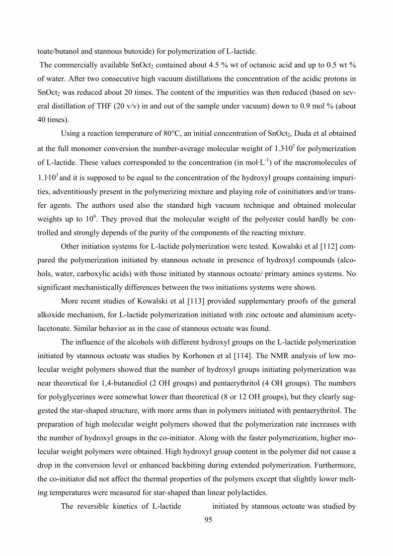
95
toate/butanol and stannous butoxide) for polymerization of L-lactide.
The commercially available SnOct2 contained about 4.5 % wt of octanoic acid and up to 0.5 wt %
of water. After two consecutive high vacuum distillations the concentration of the acidic protons in
SnOct2 was reduced about 20 times. The content of the impurities was then reduced (based on sev-
eral distillation of THF (20 v/v) in and out of the sample under vacuum) down to 0.9 mol % (about
40 times).
Using a reaction temperature of 80°C, an initial concentration of SnOct2, Duda et al obtained
at the full monomer conversion the number-average molecular weight of 51.3·10 for polymerization
of L-lactide. These values corresponded to the concentration (in mol·L-1) of the macromolecules of
31.1·10 and it is supposed to be equal to the concentration of the hydroxyl groups containing impuri-
ties, adventitiously present in the polymerizing mixture and playing role of coinitiators and/or trans-
fer agents. The authors used also the standard high vacuum technique and obtained molecular
weights up to 106. They proved that the molecular weight of the polyester could hardly be con-
trolled and strongly depends of the purity of the components of the reacting mixture.
Other initiation systems for L-lactide polymerization were tested. Kowalski et al [112] com-
pared the polymerization initiated by stannous octoate in presence of hydroxyl compounds (alco-
hols, water, carboxylic acids) with those initiated by stannous octoate/ primary amines systems. No
significant mechanistically differences between the two initiations systems were shown.
More recent studies of Kowalski et al [113] provided supplementary proofs of the general
alkoxide mechanism, for L-lactide polymerization initiated with zinc octoate and aluminium acety-
lacetonate. Similar behavior as in the case of stannous octoate was found.
The influence of the alcohols with different hydroxyl groups on the L-lactide polymerization
initiated by stannous octoate was studies by Korhonen et al [114]. The NMR analysis of low mo-
lecular weight polymers showed that the number of hydroxyl groups initiating polymerization was
near theoretical for 1,4-butanediol (2 OH groups) and pentaerythritol (4 OH groups). The numbers
for polyglycerines were somewhat lower than theoretical (8 or 12 OH groups), but they clearly sug-
gested the star-shaped structure, with more arms than in polymers initiated with pentaerythritol. The
preparation of high molecular weight polymers showed that the polymerization rate increases with
the number of hydroxyl groups in the co-initiator. Along with the faster polymerization, higher mo-
lecular weight polymers were obtained. High hydroxyl group content in the polymer did not cause a
drop in the conversion level or enhanced backbiting during extended polymerization. Furthermore,
the co-initiator did not affect the thermal properties of the polymers except that slightly lower melt-
ing temperatures were measured for star-shaped than linear polylactides.
The reversible kinetics of L-lactide initiated by stannous octoate was studied by

96
Witzke et al [115]. The propagation reaction was supposed to be reversible and the activation en-
ergy value for this reaction was calculated. The assumption that the total number of reaction centers
is equivalent to the initial number of initiator molecules was made. The equilibrium monomer con-
centrations were calculated for different operating conditions.
The first conclusion is that the hydroxyl compounds present in the polymerization mixture
have an important role in the initiation of the polymeric chains. The acidic and hydroxyl compounds
produce the deactivation of the active polymer by chain transfer resulting inactive polymer species.
A simple reaction mechanism that doesn’t take into account the reversibility of the initiator forma-
tion could contain elementary steps of initiation, propagation, chain transfer to monomer and sol-
vent.
PLA thermal and rheological properties
Like in the case of other polymers, the thermal properties of PLA are related to the structure
of the polymeric chains. Polylactides are very sensitive to heat, for temperature larger than 190 oC.
Most of degradative reactions were supposed to involve the highly concentrated ester bond on the
main chain. Low molecular weight compounds (water, monomer, oligomers, polymerization cata-
lyst) associated with the polymer seemed to play an important role in lowering molecular weights at
high temperatures [116]. The PLA chain could be considered stable for monomer amounts lower
than 2% in the final product [70, 72-74].
Even if stannous octoate can promote sufficiently fast lactide polymerization, it is also known
to have adverse effect on the PLA molecular weight and properties, as a result of backbiting and
intermolecular transesterification reactions, not only during the lactide polymerization but also dur-
ing any further melt processing [117].
Degradation studies were performed by McNeil et al [118] for a temperature range of 230 -
440 oC. The authors proposed a degradation mechanism and activation energy of 28.5 kcal/mol was
determined. The influence of an inhibitor (1,4 – diaminoantraquinone) in amount of 1 % wt on the
degradation reaction of PLA was reported. A beneficial effect of the inhibitor was observed, indi-
cating that a free radical chain process is involved in PLA degradation. A commercially available
product (ULTRANOX 626), based on Bis (2,4-di-t-butylphenyl) Pentaerythritol Diphosphite was
successfully tested by Jacobsen et al [63, 119] to stabilize a L-lactide reactive extrusion process.
The glass transition temperature (Tg) is one of the most important characteristics of a poly-
mer since it defines the operating temperature for polymer manufacturing. Variations in Tg for a
particular polymer system may reflect different molecular weights, the presence of adventitious
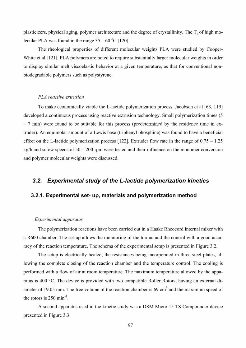
97
plasticizers, physical aging, polymer architecture and the degree of crystallinity. The Tg of high mo-
lecular PLA was found in the range 35 – 60 oC [120].
The rheological properties of different molecular weights PLA were studied by Cooper-
White et al [121]. PLA polymers are noted to require substantially larger molecular weights in order
to display similar melt viscoelastic behavior at a given temperature, as that for conventional non-
biodegradable polymers such as polystyrene.
PLA reactive extrusion
To make economically viable the L-lactide polymerization process, Jacobsen et al [63, 119]
developed a continuous process using reactive extrusion technology. Small polymerization times (5
– 7 min) were found to be suitable for this process (predetermined by the residence time in ex-
truder). An equimolar amount of a Lewis base (triphenyl phosphine) was found to have a beneficial
effect on the L-lactide polymerization process [122]. Extruder flow rate in the range of 0.75 – 1.25
kg/h and screw speeds of 50 – 200 rpm were tested and their influence on the monomer conversion
and polymer molecular weights were discussed.
3.2. Experimental study of the L-lactide polymerization kinetics
3.2.1. Experimental set- up, materials and polymerization method
Experimental apparatus
The polymerization reactions have been carried out in a Haake Rheocord internal mixer with
a R600 chamber. The set-up allows the monitoring of the torque and the control with a good accu-
racy of the reaction temperature. The schema of the experimental setup is presented in Figure 3.2.
The setup is electrically heated, the resistances being incorporated in three steel plates, al-
lowing the complete closing of the reaction chamber and the temperature control. The cooling is
performed with a flow of air at room temperature. The maximum temperature allowed by the appa-
ratus is 400 °C. The device is provided with two compatible Roller Rotors, having an external di-
ameter of 19.05 mm. The free volume of the reaction chamber is 69 cm3 and the maximum speed of
the rotors is 250 min-1.
A second apparatus used in the kinetic study was a DSM Micro 15 TS Compounder device
presented in Figure 3.3.
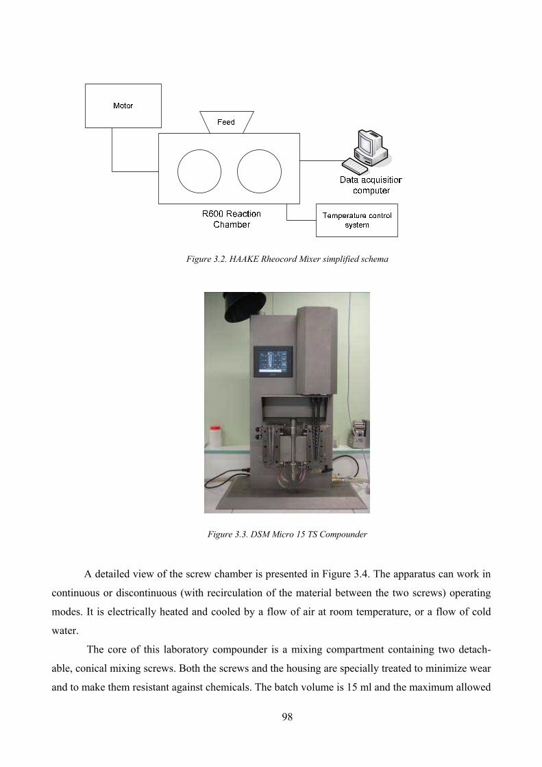
98
Figure 3.2. HAAKE Rheocord Mixer simplified schema
Figure 3.3. DSM Micro 15 TS Compounder
A detailed view of the screw chamber is presented in Figure 3.4. The apparatus can work in
continuous or discontinuous (with recirculation of the material between the two screws) operating
modes. It is electrically heated and cooled by a flow of air at room temperature, or a flow of cold
water.
The core of this laboratory compounder is a mixing compartment containing two detach-
able, conical mixing screws. Both the screws and the housing are specially treated to minimize wear
and to make them resistant against chemicals. The batch volume is 15 ml and the maximum allowed
99
temperature is 350 °C. The temperature control is possible on 6 zones, and the screw speed can be
varied between 0 to 250 rpm.
Figure 3.4. Detailed view of the reaction chamber
Materials
The L-Lactide dimer was purchased from Boehringer Ingelheim and the stannous octoate
(Sn bis-ethyl-2-hexanoate) initiator and triphenyl phosphine co-initiator from Sigma Chemicals.
One of the aims of the study was to investigate the process characteristics by using the commercial
purity L-lactide and initiator.According to the specifications of the producer, the purity of L-lactide
was minimum 99 % (wt), the heavy metals content of maximum 10 ppm, a maximum water content
of 0.02 %, free acid content 0.027% and residual solvent (toluene) maximum 0.2 %. Also a maxi-
mum percent of 0.2 % mesolactide could be found.
The purity of stannous octoate was 95%, the main impurities according to Kowalski et al
and Duda et al [111, 113, 123] being water (0.5 wt-%) and octanoic acid (4.5 wt-%). L-lactide dim-
mer, stannous octoate and triphenyl phosphine initiator were used as received, without any purify-
ing treatment. In the case of polymerization reactions co-initiated by triphenyl phosphine, the com-
pound was added in equimolecular ratio with stannous octoate.
Method
In the experiments performed on the HAAKE Mixer, a quantity of approximately 50 g mo-
nomer was fed into the reaction chamber. In order to insure a better control of the initiator quantity
it has been first dissolved in anhydrous toluene. As an example, in the experiments with the mini-
mum concentration of initiator (M/I = 4500) a volume of 0.025 ml stannous octoate has to be mixed
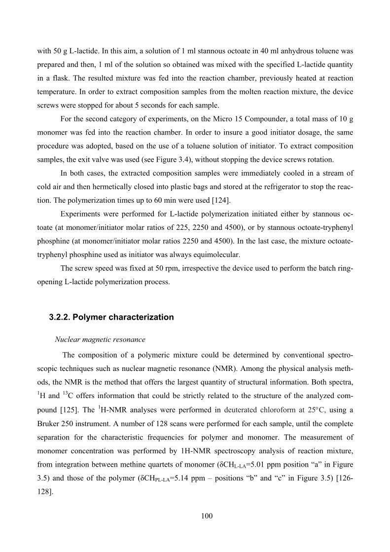
100
with 50 g L-lactide. In this aim, a solution of 1 ml stannous octoate in 40 ml anhydrous toluene was
prepared and then, 1 ml of the solution so obtained was mixed with the specified L-lactide quantity
in a flask. The resulted mixture was fed into the reaction chamber, previously heated at reaction
temperature. In order to extract composition samples from the molten reaction mixture, the device
screws were stopped for about 5 seconds for each sample.
For the second category of experiments, on the Micro 15 Compounder, a total mass of 10 g
monomer was fed into the reaction chamber. In order to insure a good initiator dosage, the same
procedure was adopted, based on the use of a toluene solution of initiator. To extract composition
samples, the exit valve was used (see Figure 3.4), without stopping the device screws rotation.
In both cases, the extracted composition samples were immediately cooled in a stream of
cold air and then hermetically closed into plastic bags and stored at the refrigerator to stop the reac-
tion. The polymerization times up to 60 min were used [124].
Experiments were performed for L-lactide polymerization initiated either by stannous oc-
toate (at monomer/initiator molar ratios of 225, 2250 and 4500), or by stannous octoate-tryphenyl
phosphine (at monomer/initiator molar ratios 2250 and 4500). In the last case, the mixture octoate-
tryphenyl phosphine used as initiator was always equimolecular.
The screw speed was fixed at 50 rpm, irrespective the device used to perform the batch ring-
opening L-lactide polymerization process.
3.2.2. Polymer characterization
Nuclear magnetic resonance
The composition of a polymeric mixture could be determined by conventional spectro-
scopic techniques such as nuclear magnetic resonance (NMR). Among the physical analysis meth-
ods, the NMR is the method that offers the largest quantity of structural information. Both spectra, 1H and 13C offers information that could be strictly related to the structure of the analyzed com-
pound [125]. The 1H-NMR analyses were performed in deuterated chloroform at 25°C, using a
Bruker 250 instrument. A number of 128 scans were performed for each sample, until the complete
separation for the characteristic frequencies for polymer and monomer. The measurement of
monomer concentration was performed by 1H-NMR spectroscopy analysis of reaction mixture,
from integration between methine quartets of monomer (hCHL-LA=5.01 ppm position “a” in Figure
3.5) and those of the polymer (hCHPL-LA=5.14 ppm – positions “b” and “c” in Figure 3.5) [126-
128].
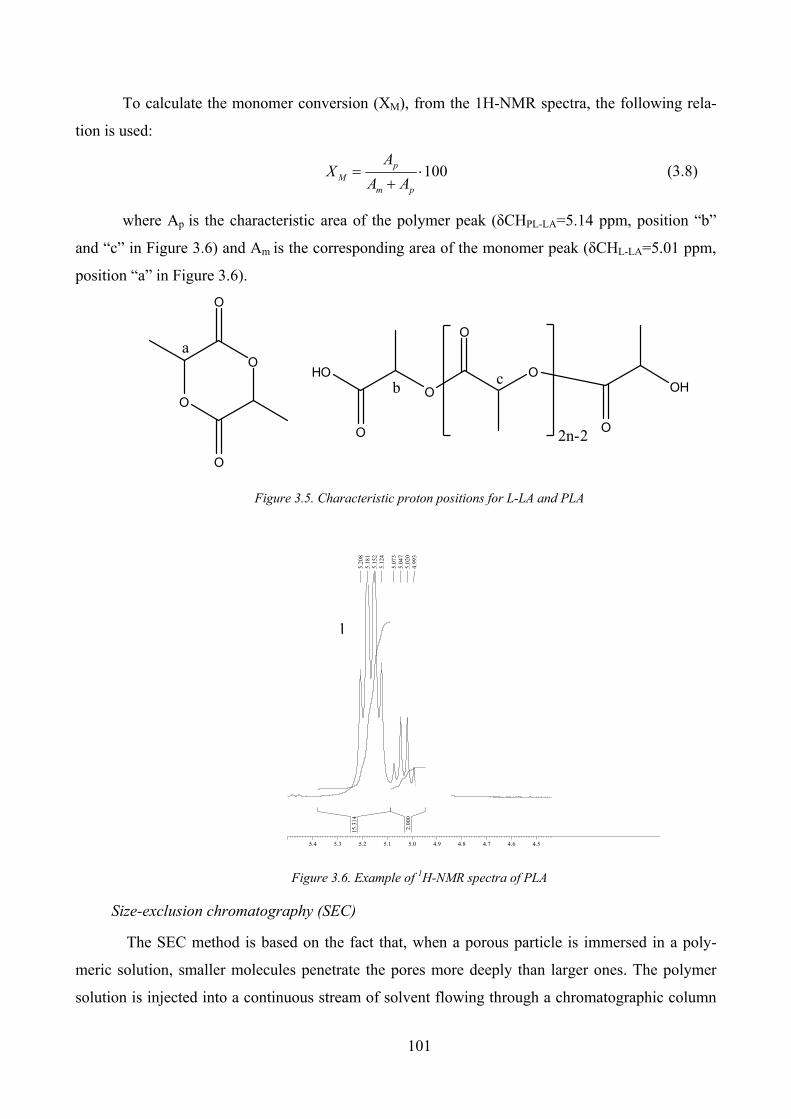
101
To calculate the monomer conversion (XM), from the 1H-NMR spectra, the following rela-
tion is used:
100p
M
m p
AX
A A= ⋅+ (3.8)
where Ap is the characteristic area of the polymer peak (hCHPL-LA=5.14 ppm, position “b”
and “c” in Figure 3.6) and Am is the corresponding area of the monomer peak (hCHL-LA=5.01 ppm,
position “a” in Figure 3.6).
O
O
O
O
HO
O
O
O
O
O
OH
2n-2
a
bc
Figure 3.5. Characteristic proton positions for L-LA and PLA
4.54.64.74.84.95.05.15.25.35.4
4.99
35.
020
5.04
75.
073
5.12
45.
152
5.18
15.
208
2.00
0
15.3
14
Figure 3.6. Example of 1H-NMR spectra of PLA
Size-exclusion chromatography (SEC)
The SEC method is based on the fact that, when a porous particle is immersed in a poly-
meric solution, smaller molecules penetrate the pores more deeply than larger ones. The polymer
solution is injected into a continuous stream of solvent flowing through a chromatographic column
b

102
filled with a porous material. Since the dimension of a macromolecule reflects its molar mass,
polymer molecules which possess low masses are eluted by the flowing solvent at later times. The
SEC measurements have been performed at 30°C using chloroform as solvent and a solution of 5
mg/ml of L-lactide, on a Waters 510 apparatus using a Polymer Laboratory PLGel 5 μm Mixed-C
column. The detector was a Waters 410 differential refractometer, and the scaling has been made
using polystyrene standards provided by PolymerLab. A flow rate of 1 mL/min (total time of 12
minutes) was used for each analysis. The method was used to determine the molecular weight dis-
tribution and the mean-molecular weights of the polymers.
It is known from the published literature that, for a given temperature and solvent, at any
given retention volume, it is fulfilled the relation [129]:
PLA PLA PS PSM Mη = η (3.9)
Where PS denotes the polystyrene standard, PLA denotes the working polymer (polylac-
tide), η – the intrinsic viscosity of the polymer solution and M is the molecular weight of the poly-
mer. The viscosity is generally represented by a Mark-Houwink equation:
K M αη = ⋅ (3.10)
Published values of Mark-Houwink parameters in common SEC solvents are available for
many polymers. If Mark-Houwink constants (K and α) for the analyzed polymer and for the stan-
dard are known, from equations (3.10) and (3.9) one obtains:
( )PLA
PS1/ 11
PS PSPLA
PLA
K MM
K
α +α +⎛ ⎞⎜ ⎟= ⎜ ⎟⎝ ⎠ (3.11)
In our determinations, the Mark-Houwink constants were: for polystyrene: KPS = 1.64·10-4,
αPS = 0.692 and for polylactide, KPLA = 1.05·10-3, αPLA = 0.563 [119].
The accuracy of the molecular weights determination by SEC is in the range ±5 % as re-
ported in the published literature [130]. An example of PLA chromatogram is presented in Figure
3.7. The high peak on the right is characteristic to un-reacted monomer (small molecular weight
species) and the other is characteristic for the polymeric (high molecular weight species) products in
the reaction mixture [131].
This method, usually used for determination of molecular weights and molecular weights
distributions, also permits the determination of the monomer conversion in this case, by using the
peak areas for polymers (Ap) and the corresponding area for monomer (Am). The relation used to
calculate the monomer conversion (XM) is [131]:
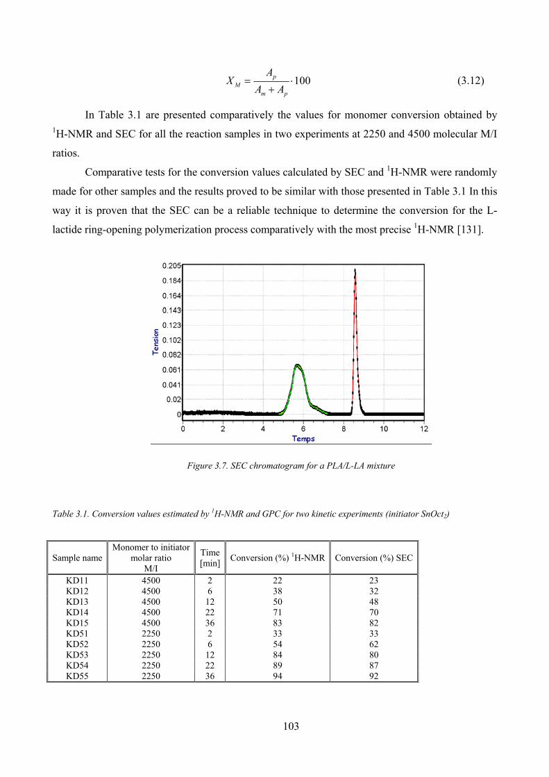
103
100p
M
m p
AX
A A= ⋅+ (3.12)
In Table 3.1 are presented comparatively the values for monomer conversion obtained by 1H-NMR and SEC for all the reaction samples in two experiments at 2250 and 4500 molecular M/I
ratios.
Comparative tests for the conversion values calculated by SEC and 1H-NMR were randomly
made for other samples and the results proved to be similar with those presented in Table 3.1 In this
way it is proven that the SEC can be a reliable technique to determine the conversion for the L-
lactide ring-opening polymerization process comparatively with the most precise 1H-NMR [131].
Figure 3.7. SEC chromatogram for a PLA/L-LA mixture
Table 3.1. Conversion values estimated by 1H-NMR and GPC for two kinetic experiments (initiator SnOct2)
Sample name Monomer to initiator
molar ratio M/I
Time [min]
Conversion (%) 1H-NMR Conversion (%) SEC
KD11 4500 2 22 23 KD12 4500 6 38 32 KD13 4500 12 50 48 KD14 4500 22 71 70 KD15 4500 36 83 82 KD51 2250 2 33 33 KD52 2250 6 54 62 KD53 2250 12 84 80 KD54 2250 22 89 87 KD55 2250 36 94 92
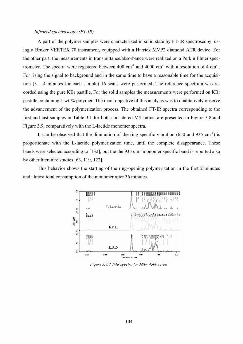
104
Infrared spectroscopy (FT-IR)
A part of the polymer samples were characterized in solid state by FT-IR spectroscopy, us-
ing a Bruker VERTEX 70 instrument, equipped with a Harrick MVP2 diamond ATR device. For
the other part, the measurements in transmittance/absorbance were realized on a Perkin Elmer spec-
trometer. The spectra were registered between 400 cm-1 and 4000 cm-1 with a resolution of 4 cm-1.
For rising the signal to background and in the same time to have a reasonable time for the acquisi-
tion (3 – 4 minutes for each sample) 16 scans were performed. The reference spectrum was re-
corded using the pure KBr pastille. For the solid samples the measurements were performed on KBr
pastille containing 1 wt-% polymer. The main objective of this analysis was to qualitatively observe
the advancement of the polymerization process. The obtained FT-IR spectra corresponding to the
first and last samples in Table 3.1 for both considered M/I ratios, are presented in Figure 3.8 and
Figure 3.9, comparatively with the L-lactide monomer spectra.
It can be observed that the diminution of the ring specific vibration (650 and 935 cm-1) is
proportionate with the L-lactide polymerization time, until the complete disappearance. These
bands were selected according to [132], but the the 935 cm-1 monomer specific band is reported also
by other literature studies [63, 119, 122].
This behavior shows the starting of the ring-opening polymerization in the first 2 minutes
and almost total consumption of the monomer after 36 minutes.
Figure 3.8. FT-IR spectra for M/I= 4500 series
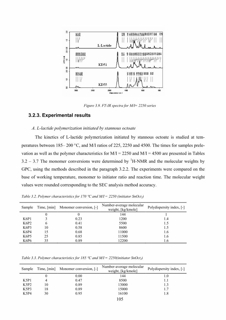
105
Figure 3.9. FT-IR spectra for M/I= 2250 series
3.2.3. Experimental results
A. L-lactide polymerization initiated by stannous octoate
The kinetics of L-lactide polymerization initiated by stannous octoate is studied at tem-
peratures between 185– 200 °C, and M/I ratios of 225, 2250 and 4500. The times for samples prele-
vation as well as the polymer characteristics for M/I = 2250 and M/I = 4500 are presented in Tables
3.2 – 3.7 The monomer conversions were determined by 1H-NMR and the molecular weights by
GPC, using the methods described in the paragraph 3.2.2. The experiments were compared on the
base of working temperature, monomer to initiator ratio and reaction time. The molecular weight
values were rounded corresponding to the SEC analysis method accuracy.
Table 3.2. Polymer characteristics for 170 °C and M/I = 2250 (initiator SnOct2)
Sample Time, [min] Monomer conversion, [-] Number-average molecular
weight, [kg/kmole] Polydispersity index, [-]
0 0 144 1 K6P1 3 0.23 1200 1.4 K6P2 6 0.41 5500 1.5 K6P3 10 0.58 8600 1.5 K6P4 15 0.68 11000 1.6 K6P5 25 0.85 11500 1.6 K6P6 35 0.89 12200 1.6
Table 3.3. Polymer characteristics for 185 °C and M/I = 2250(initiator SnOct2)
Sample Time, [min] Monomer conversion, [-] Number-average molecular
weight, [kg/kmole] Polydispersity index, [-]
0 0.00 144 1.0 K5P1 4 0.47 8500 1.1 K5P2 10 0.89 13000 1.3 K5P3 18 0.89 15000 1.7 K5P4 30 0.95 16100 1.8
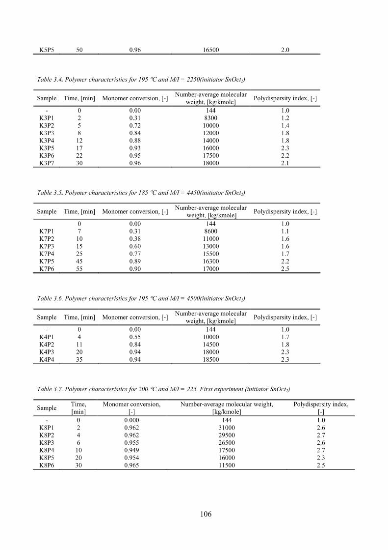
106
K5P5 50 0.96 16500 2.0
Table 3.4. Polymer characteristics for 195 °C and M/I = 2250(initiator SnOct2)
Sample Time, [min] Monomer conversion, [-] Number-average molecular
weight, [kg/kmole] Polydispersity index, [-]
- 0 0.00 144 1.0 K3P1 2 0.31 8300 1.2 K3P2 5 0.72 10000 1.4 K3P3 8 0.84 12000 1.8 K3P4 12 0.88 14000 1.8 K3P5 17 0.93 16000 2.3 K3P6 22 0.95 17500 2.2 K3P7 30 0.96 18000 2.1
Table 3.5. Polymer characteristics for 185 °C and M/I = 4450(initiator SnOct2)
Sample Time, [min] Monomer conversion, [-] Number-average molecular
weight, [kg/kmole] Polydispersity index, [-]
0 0.00 144 1.0 K7P1 7 0.31 8600 1.1 K7P2 10 0.38 11000 1.6 K7P3 15 0.60 13000 1.6 K7P4 25 0.77 15500 1.7 K7P5 45 0.89 16300 2.2 K7P6 55 0.90 17000 2.5
Table 3.6. Polymer characteristics for 195 °C and M/I = 4500(initiator SnOct2)
Sample Time, [min] Monomer conversion, [-] Number-average molecular
weight, [kg/kmole] Polydispersity index, [-]
- 0 0.00 144 1.0 K4P1 4 0.55 10000 1.7 K4P2 11 0.84 14500 1.8 K4P3 20 0.94 18000 2.3 K4P4 35 0.94 18500 2.3
Table 3.7. Polymer characteristics for 200 °C and M/I = 225. First experiment (initiator SnOct2)
Sample Time, [min]
Monomer conversion, [-]
Number-average molecular weight, [kg/kmole]
Polydispersity index, [-]
- 0 0.000 144 1.0 K8P1 2 0.962 31000 2.6 K8P2 4 0.962 29500 2.7 K8P3 6 0.955 26500 2.6 K8P4 10 0.949 17500 2.7 K8P5 20 0.954 16000 2.3 K8P6 30 0.965 11500 2.5

107
Table 3.8. Polymer characteristics for 200 °C and M/I = 225. Second experiment (initiator SnOct2)
Sample Time, [min]
Monomer conversion, [-]
Number-average molecular weight, [kg/kmole]
Polydispersity index, [-]
- 0 0.000 144 1.0 K9P1 2 0.950 31500 2.6 K9P2 4 0.965 29000 2.7 K9P3 6 0.952 26000 2.6 K9P4 10 0.951 17000 2.8 K9P5 20 0.957 16500 2.4
To check the reproducibility of L-lactide polymerization data, several experiments were re-
peated in identical working conditions. The results showed a good reproducibility of data all over
the working domain. An excerpt of these is given in Tables 3.7 and 3.8. As seen from Table 3.7,
working at high temperature and high initiator concentration, almost complete monomer conversion
values are obtained after only 2 minutes of polymerization time. The high initiator concentration
promotes the formation of numerous polymeric chains, and the propagation rate rise proportionally
to their concentration, providing the high monomer conversions. An explanation for the decrease in
polymer molecular weights after 2 minutes could be a significant termination rate corroborated with
a depolymerization process, due to the high temperature in the polymerization reactor.
In spite of the relatively large scatter of experimental points, the data presented in Tables 3.2
– 3.6 permit to draw several conclusions regarding the L-lactide polymerization process. An impor-
tant conclusion is that the bulk polymerization process cannot be conducted at reactions times of the
same order of magnitude as the residence times of the melts in twin-screw extruders. However, the
use of industrial TSE with longer residence times can be envisaged. Also, the values of molecular
weights of the polymers are particularly low, insufficient to produce a polymer of practical interest.
As already mentioned, several previous studies showed a weak reversibility of L-lactide po-
lymerization [110, 115]. This particularity could explain the fact that the conversion curves tend to
plateau out on the last time interval and the time dependence of Mn at high temperatures present an
evolution with a weak maximum.
Temperature influence
It is well known that the temperature has an enhancing effect on the propagation rates, but
also augments the side reactions, as de-polymerization and inter and intra-molecular transes-
terification. The temperature dependence of monomer conversion and number average molecular
weight, for two monomer/initiator molecular ratios, is presented in Figures 3.10 and 3.11.
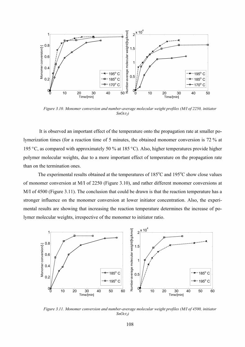
108
Figure 3.10. Monomer conversion and number-average molecular weight profiles (M/I of 2250, initiator
SnOct2)
It is observed an important effect of the temperature onto the propagation rate at smaller po-
lymerization times (for a reaction time of 5 minutes, the obtained monomer conversion is 72 % at
195 °C, as compared with approximately 50 % at 185 °C). Also, higher temperatures provide higher
polymer molecular weights, due to a more important effect of temperature on the propagation rate
than on the termination ones.
The experimental results obtained at the temperatures of 185oC and 195oC show close values
of monomer conversion at M/I of 2250 (Figure 3.10), and rather different monomer conversions at
M/I of 4500 (Figure 3.11). The conclusion that could be drawn is that the reaction temperature has a
stronger influence on the monomer conversion at lower initiator concentration. Also, the experi-
mental results are showing that increasing the reaction temperature determines the increase of po-
lymer molecular weights, irrespective of the monomer to initiator ratio.
Figure 3.11. Monomer conversion and number-average molecular weight profiles (M/I of 4500, initiator
SnOct2)
0 10 20 30 40 500
0.2
0.4
0.6
0.8
1
Time/[min]
Mo
no
me
r co
nve
rsio
n/[-]
195o C
185o C
170o C
0 10 20 30 40 500
0.5
1
1.5
2x 10
4
Time/[min]
Nu
mb
er-
ave
rag
e m
ole
cu
lar
we
igh
t/[k
g/k
mo
l]
195o C
185o C
170o C
0 10 20 30 40 50 600
0.2
0.4
0.6
0.8
1
Time/[min]
Mo
no
me
r co
nve
rsio
n/[-]
185o C
195o C
0 10 20 30 40 50 600
0.5
1
1.5
2x 10
4
Time/[min]
Nu
mb
er-
ave
rag
e m
ole
cu
lar
we
igh
t/[k
g/k
mo
l]
185o C
195o C
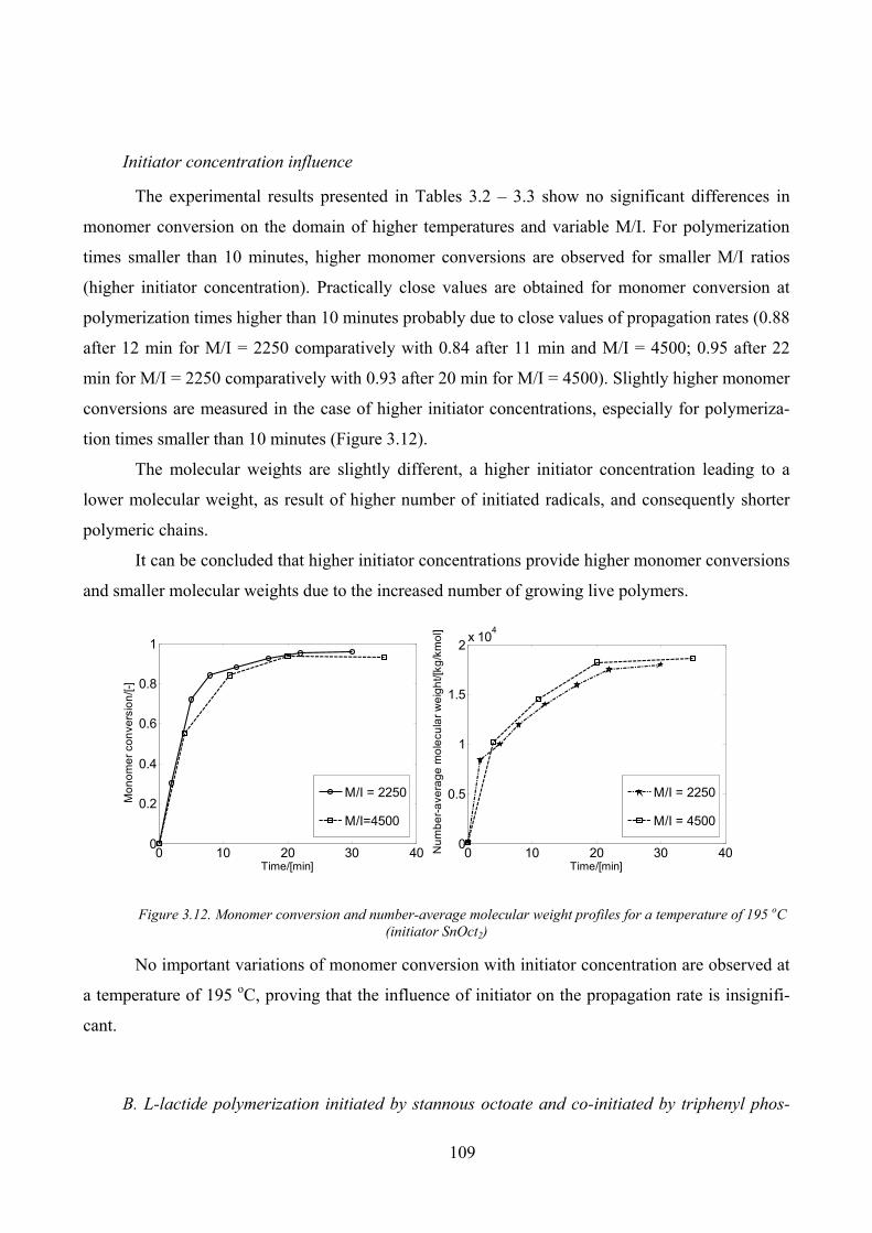
109
Initiator concentration influence
The experimental results presented in Tables 3.2 – 3.3 show no significant differences in
monomer conversion on the domain of higher temperatures and variable M/I. For polymerization
times smaller than 10 minutes, higher monomer conversions are observed for smaller M/I ratios
(higher initiator concentration). Practically close values are obtained for monomer conversion at
polymerization times higher than 10 minutes probably due to close values of propagation rates (0.88
after 12 min for M/I = 2250 comparatively with 0.84 after 11 min and M/I = 4500; 0.95 after 22
min for M/I = 2250 comparatively with 0.93 after 20 min for M/I = 4500). Slightly higher monomer
conversions are measured in the case of higher initiator concentrations, especially for polymeriza-
tion times smaller than 10 minutes (Figure 3.12).
The molecular weights are slightly different, a higher initiator concentration leading to a
lower molecular weight, as result of higher number of initiated radicals, and consequently shorter
polymeric chains.
It can be concluded that higher initiator concentrations provide higher monomer conversions
and smaller molecular weights due to the increased number of growing live polymers.
Figure 3.12. Monomer conversion and number-average molecular weight profiles for a temperature of 195 oC
(initiator SnOct2)
No important variations of monomer conversion with initiator concentration are observed at
a temperature of 195 oC, proving that the influence of initiator on the propagation rate is insignifi-
cant.
B. L-lactide polymerization initiated by stannous octoate and co-initiated by triphenyl phos-
0 10 20 30 400
0.2
0.4
0.6
0.8
1
Time/[min]
Mo
no
me
r co
nve
rsio
n/[-]
M/I = 2250
M/I=4500
0 10 20 30 400
0.5
1
1.5
2x 10
4
Time/[min]
Nu
mb
er-
ave
rag
e m
ole
cu
lar
we
igh
t/[k
g/k
mo
l]
M/I = 2250
M/I = 4500
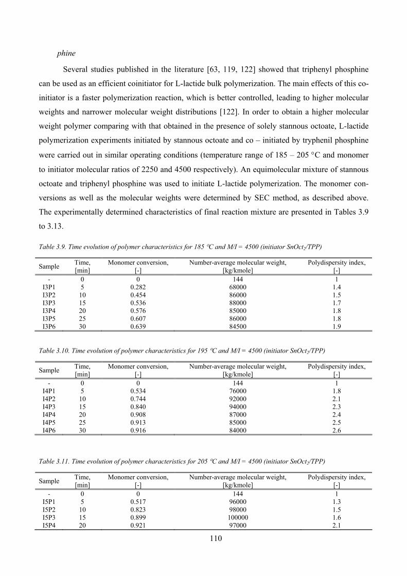
110
phine
Several studies published in the literature [63, 119, 122] showed that triphenyl phosphine
can be used as an efficient coinitiator for L-lactide bulk polymerization. The main effects of this co-
initiator is a faster polymerization reaction, which is better controlled, leading to higher molecular
weights and narrower molecular weight distributions [122]. In order to obtain a higher molecular
weight polymer comparing with that obtained in the presence of solely stannous octoate, L-lactide
polymerization experiments initiated by stannous octoate and co – initiated by tryphenil phosphine
were carried out in similar operating conditions (temperature range of 185 – 205 °C and monomer
to initiator molecular ratios of 2250 and 4500 respectively). An equimolecular mixture of stannous
octoate and triphenyl phosphine was used to initiate L-lactide polymerization. The monomer con-
versions as well as the molecular weights were determined by SEC method, as described above.
The experimentally determined characteristics of final reaction mixture are presented in Tables 3.9
to 3.13.
Table 3.9. Time evolution of polymer characteristics for 185 °C and M/I = 4500 (initiator SnOct2/TPP)
Sample Time, [min]
Monomer conversion, [-]
Number-average molecular weight, [kg/kmole]
Polydispersity index, [-]
- 0 0 144 1 I3P1 5 0.282 68000 1.4 I3P2 10 0.454 86000 1.5 I3P3 15 0.536 88000 1.7 I3P4 20 0.576 85000 1.8 I3P5 25 0.607 86000 1.8 I3P6 30 0.639 84500 1.9
Table 3.10. Time evolution of polymer characteristics for 195 °C and M/I = 4500 (initiator SnOct2/TPP)
Sample Time, [min]
Monomer conversion, [-]
Number-average molecular weight, [kg/kmole]
Polydispersity index, [-]
- 0 0 144 1 I4P1 5 0.534 76000 1.8 I4P2 10 0.744 92000 2.1 I4P3 15 0.840 94000 2.3 I4P4 20 0.908 87000 2.4 I4P5 25 0.913 85000 2.5 I4P6 30 0.916 84000 2.6
Table 3.11. Time evolution of polymer characteristics for 205 °C and M/I = 4500 (initiator SnOct2/TPP)
Sample Time, [min]
Monomer conversion, [-]
Number-average molecular weight, [kg/kmole]
Polydispersity index, [-]
- 0 0 144 1 I5P1 5 0.517 96000 1.3 I5P2 10 0.823 98000 1.5 I5P3 15 0.899 100000 1.6 I5P4 20 0.921 97000 2.1
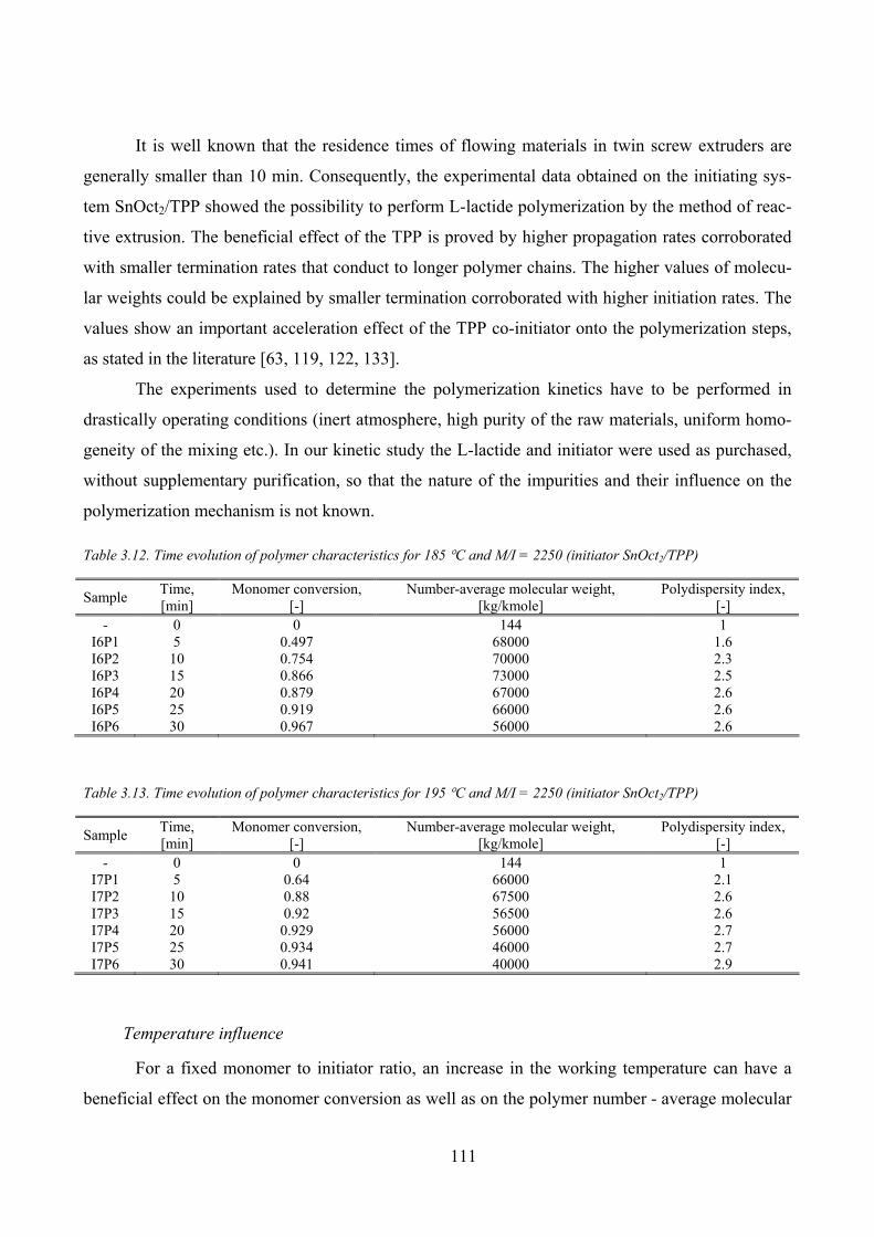
111
It is well known that the residence times of flowing materials in twin screw extruders are
generally smaller than 10 min. Consequently, the experimental data obtained on the initiating sys-
tem SnOct2/TPP showed the possibility to perform L-lactide polymerization by the method of reac-
tive extrusion. The beneficial effect of the TPP is proved by higher propagation rates corroborated
with smaller termination rates that conduct to longer polymer chains. The higher values of molecu-
lar weights could be explained by smaller termination corroborated with higher initiation rates. The
values show an important acceleration effect of the TPP co-initiator onto the polymerization steps,
as stated in the literature [63, 119, 122, 133].
The experiments used to determine the polymerization kinetics have to be performed in
drastically operating conditions (inert atmosphere, high purity of the raw materials, uniform homo-
geneity of the mixing etc.). In our kinetic study the L-lactide and initiator were used as purchased,
without supplementary purification, so that the nature of the impurities and their influence on the
polymerization mechanism is not known.
Table 3.12. Time evolution of polymer characteristics for 185 °C and M/I = 2250 (initiator SnOct2/TPP)
Sample Time, [min]
Monomer conversion, [-]
Number-average molecular weight, [kg/kmole]
Polydispersity index, [-]
- 0 0 144 1 I6P1 5 0.497 68000 1.6 I6P2 10 0.754 70000 2.3 I6P3 15 0.866 73000 2.5 I6P4 20 0.879 67000 2.6 I6P5 25 0.919 66000 2.6 I6P6 30 0.967 56000 2.6
Table 3.13. Time evolution of polymer characteristics for 195 °C and M/I = 2250 (initiator SnOct2/TPP)
Sample Time, [min]
Monomer conversion, [-]
Number-average molecular weight, [kg/kmole]
Polydispersity index, [-]
- 0 0 144 1 I7P1 5 0.64 66000 2.1 I7P2 10 0.88 67500 2.6 I7P3 15 0.92 56500 2.6 I7P4 20 0.929 56000 2.7 I7P5 25 0.934 46000 2.7 I7P6 30 0.941 40000 2.9
Temperature influence
For a fixed monomer to initiator ratio, an increase in the working temperature can have a
beneficial effect on the monomer conversion as well as on the polymer number - average molecular
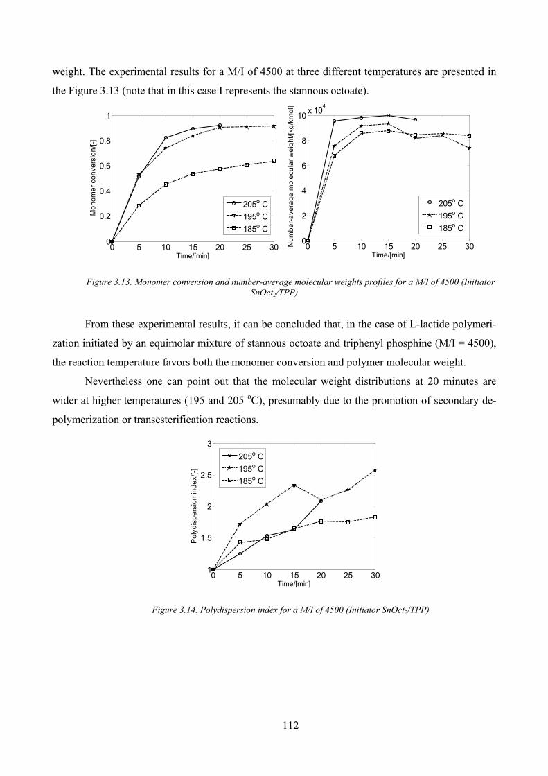
112
weight. The experimental results for a M/I of 4500 at three different temperatures are presented in
the Figure 3.13 (note that in this case I represents the stannous octoate).
Figure 3.13. Monomer conversion and number-average molecular weights profiles for a M/I of 4500 (Initiator
SnOct2/TPP)
From these experimental results, it can be concluded that, in the case of L-lactide polymeri-
zation initiated by an equimolar mixture of stannous octoate and triphenyl phosphine (M/I = 4500),
the reaction temperature favors both the monomer conversion and polymer molecular weight.
Nevertheless one can point out that the molecular weight distributions at 20 minutes are
wider at higher temperatures (195 and 205 oC), presumably due to the promotion of secondary de-
polymerization or transesterification reactions.
0 5 10 15 20 25 301
1.5
2
2.5
3
Time/[min]
Po
lyd
isp
ers
ion
in
de
x/[-]
205o C
195o C
185o C
Figure 3.14. Polydispersion index for a M/I of 4500 (Initiator SnOct2/TPP)
0 5 10 15 20 25 300
0.2
0.4
0.6
0.8
1
Time/[min]
Mo
no
me
r co
nve
rsio
n/[-]
205o C
195o C
185o C
0 5 10 15 20 25 300
2
4
6
8
10x 10
4
Time/[min]
Nu
mb
er-
ave
rag
e m
ole
cu
lar
we
igh
t/[k
g/k
mo
l]
205o C
195o C
185o C
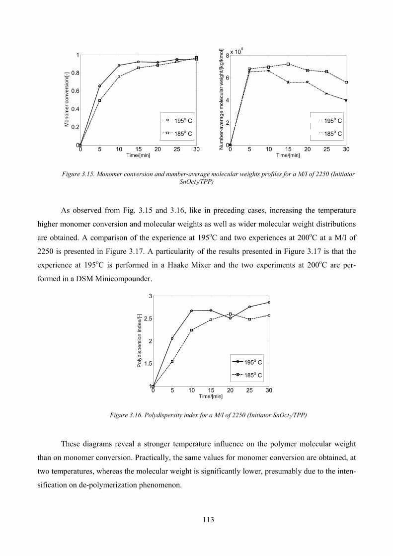
113
Figure 3.15. Monomer conversion and number-average molecular weights profiles for a M/I of 2250 (Initiator
SnOct2/TPP)
As observed from Fig. 3.15 and 3.16, like in preceding cases, increasing the temperature
higher monomer conversion and molecular weights as well as wider molecular weight distributions
are obtained. A comparison of the experience at 195oC and two experiences at 200oC at a M/I of
2250 is presented in Figure 3.17. A particularity of the results presented in Figure 3.17 is that the
experience at 195oC is performed in a Haake Mixer and the two experiments at 200oC are per-
formed in a DSM Minicompounder.
0 5 10 15 20 25 301
1.5
2
2.5
3
Time/[min]
Po
lyd
isp
ers
ion
in
de
x/[-]
195o C
185o C
Figure 3.16. Polydispersity index for a M/I of 2250 (Initiator SnOct2/TPP)
These diagrams reveal a stronger temperature influence on the polymer molecular weight
than on monomer conversion. Practically, the same values for monomer conversion are obtained, at
two temperatures, whereas the molecular weight is significantly lower, presumably due to the inten-
sification on de-polymerization phenomenon.
0 5 10 15 20 25 300
0.2
0.4
0.6
0.8
1
Time/[min]
Mo
no
me
r co
nve
rsio
n/[-]
195o C
185o C
0 5 10 15 20 25 300
2
4
6
8x 10
4
Time/[min]
Nu
mb
er-
ave
rag
e m
ole
cu
lar
we
igh
t/[k
g/k
mo
l]
195o C
185o C
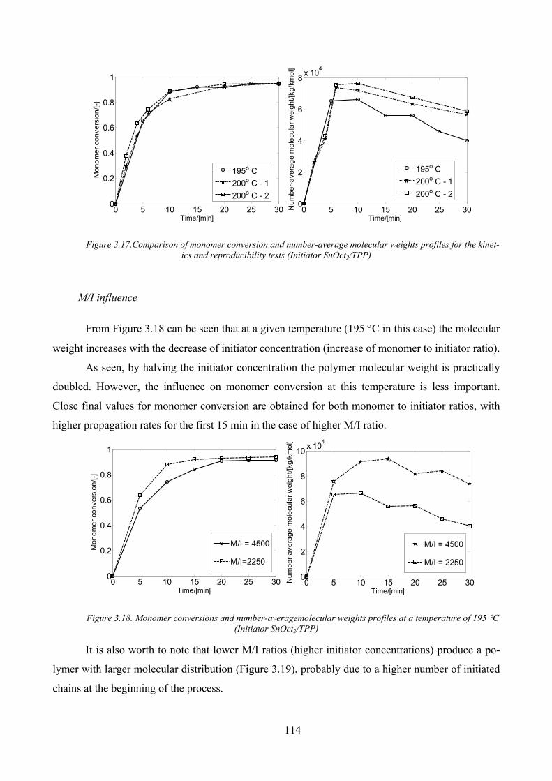
114
Figure 3.17.Comparison of monomer conversion and number-average molecular weights profiles for the kinet-
ics and reproducibility tests (Initiator SnOct2/TPP)
M/I influence
From Figure 3.18 can be seen that at a given temperature (195 °C in this case) the molecular
weight increases with the decrease of initiator concentration (increase of monomer to initiator ratio).
As seen, by halving the initiator concentration the polymer molecular weight is practically
doubled. However, the influence on monomer conversion at this temperature is less important.
Close final values for monomer conversion are obtained for both monomer to initiator ratios, with
higher propagation rates for the first 15 min in the case of higher M/I ratio.
Figure 3.18. Monomer conversions and number-averagemolecular weights profiles at a temperature of 195 °C
(Initiator SnOct2/TPP)
It is also worth to note that lower M/I ratios (higher initiator concentrations) produce a po-
lymer with larger molecular distribution (Figure 3.19), probably due to a higher number of initiated
chains at the beginning of the process.
0 5 10 15 20 25 300
0.2
0.4
0.6
0.8
1
Time/[min]
Mo
no
me
r co
nve
rsio
n/[-]
M/I = 4500
M/I=2250
0 5 10 15 20 25 300
2
4
6
8
10x 10
4
Time/[min]
Nu
mb
er-
ave
rag
e m
ole
cu
lar
we
igh
t/[k
g/k
mo
l]
M/I = 4500
M/I = 2250
0 5 10 15 20 25 300
0.2
0.4
0.6
0.8
1
Time/[min]
Mo
no
me
r co
nve
rsio
n/[-]
195o C
200o C - 1
200o C - 2
0 5 10 15 20 25 300
2
4
6
8x 10
4
Time/[min]
Nu
mb
er-
ave
rag
e m
ole
cu
lar
we
igh
t/[k
g/k
mo
l]
195o C
200o C - 1
200o C - 2
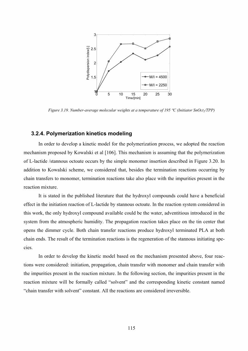
115
0 5 10 15 20 25 301
1.5
2
2.5
3
Time/[min]
Po
lyd
isp
ers
ion
in
de
x/[-]
M/I = 4500
M/I = 2250
Figure 3.19. Number-average molecular weights at a temperature of 195 °C (Initiator SnOct2/TPP)
3.2.4. Polymerization kinetics modeling
In order to develop a kinetic model for the polymerization process, we adopted the reaction
mechanism proposed by Kowalski et al [106]. This mechanism is assuming that the polymerization
of L-lactide /stannous octoate occurs by the simple monomer insertion described in Figure 3.20. In
addition to Kowalski scheme, we considered that, besides the termination reactions occurring by
chain transfers to monomer, termination reactions take also place with the impurities present in the
reaction mixture.
It is stated in the published literature that the hydroxyl compounds could have a beneficial
effect in the initiation reaction of L-lactide by stannous octoate. In the reaction system considered in
this work, the only hydroxyl compound available could be the water, adventitious introduced in the
system from the atmospheric humidity. The propagation reaction takes place on the tin center that
opens the dimmer cycle. Both chain transfer reactions produce hydroxyl terminated PLA at both
chain ends. The result of the termination reactions is the regeneration of the stannous initiating spe-
cies.
In order to develop the kinetic model based on the mechanism presented above, four reac-
tions were considered: initiation, propagation, chain transfer with monomer and chain transfer with
the impurities present in the reaction mixture. In the following section, the impurities present in the
reaction mixture will be formally called “solvent” and the corresponding kinetic constant named
“chain transfer with solvent” constant. All the reactions are considered irreversible.
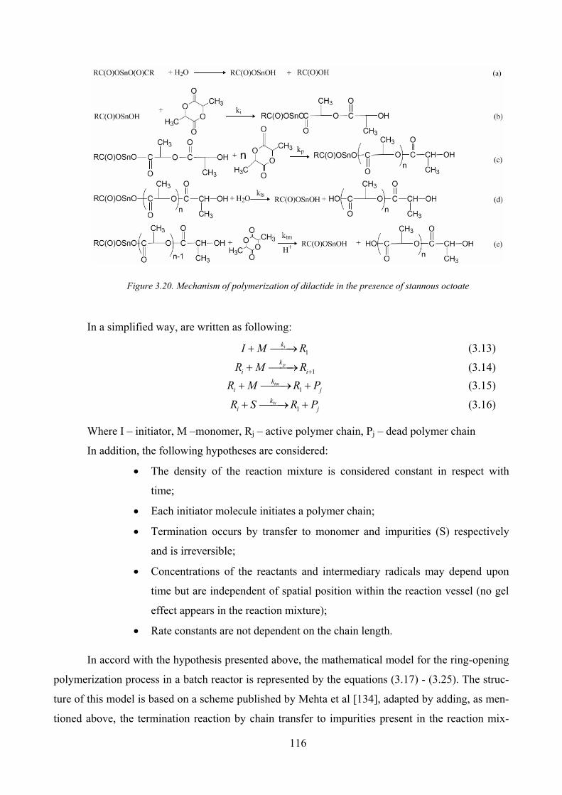
116
Figure 3.20. Mechanism of polymerization of dilactide in the presence of stannous octoate
In a simplified way, are written as following:
1ik
I M R+ ⎯⎯→ (3.13)
1pk
i iR M R ++ ⎯⎯→ (3.14)
1tmk
i jR M R P+ ⎯⎯→ + (3.15)
1tsk
i jR S R P+ ⎯⎯→ + (3.16)
Where I – initiator, M –monomer, Rj – active polymer chain, Pj – dead polymer chain
In addition, the following hypotheses are considered:
• The density of the reaction mixture is considered constant in respect with
time;
• Each initiator molecule initiates a polymer chain;
• Termination occurs by transfer to monomer and impurities (S) respectively
and is irreversible;
• Concentrations of the reactants and intermediary radicals may depend upon
time but are independent of spatial position within the reaction vessel (no gel
effect appears in the reaction mixture);
• Rate constants are not dependent on the chain length.
In accord with the hypothesis presented above, the mathematical model for the ring-opening
polymerization process in a batch reactor is represented by the equations (3.17) - (3.25). The struc-
ture of this model is based on a scheme published by Mehta et al [134], adapted by adding, as men-
tioned above, the termination reaction by chain transfer to impurities present in the reaction mix-
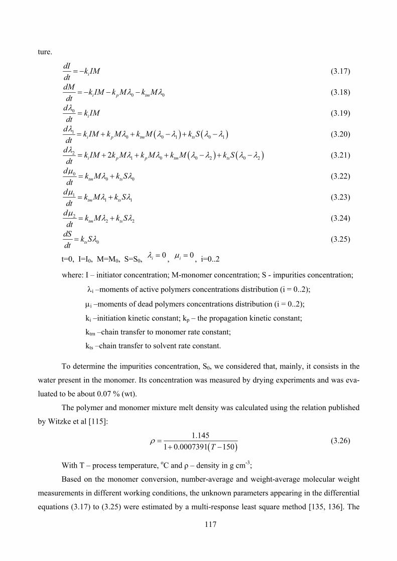
117
ture.
i
dIk IM
dt= − (3.17)
0 0i p tm
dMk IM k M k M
dtλ λ= − − − (3.18)
0i
dk IM
dt
λ = (3.19)
( ) ( )10 0 1 0 1i p tm ts
dk IM k M k M k S
dt
λ λ λ λ λ λ= + + − + − (3.20)
( ) ( )21 0 0 2 0 22i p p tm ts
dk IM k M k M k M k S
dt
λ λ λ λ λ λ λ= + + + − + − (3.21)
00 0tm ts
dk M k S
dt
μ λ λ= + (3.22)
11 1tm ts
dk M k S
dt
μ λ λ= + (3.23)
22 2tm ts
dk M k S
dt
μ λ λ= + (3.24)
0ts
dSk S
dtλ= (3.25)
t=0, I=I0, M=M0, S=S0, 0iλ = , 0iμ = , i=0..2
where: I – initiator concentration; M-monomer concentration; S - impurities concentration;
λi –moments of active polymers concentrations distribution (i = 0..2);
μi –moments of dead polymers concentrations distribution (i = 0..2);
ki –initiation kinetic constant; kp – the propagation kinetic constant;
ktm –chain transfer to monomer rate constant;
kts –chain transfer to solvent rate constant.
To determine the impurities concentration, S0, we considered that, mainly, it consists in the
water present in the monomer. Its concentration was measured by drying experiments and was eva-
luated to be about 0.07 % (wt).
The polymer and monomer mixture melt density was calculated using the relation published
by Witzke et al [115]:
( )1.145
1 0.0007391 150Tρ = + − (3.26)
With T – process temperature, oC and ρ – density in g cm-3;
Based on the monomer conversion, number-average and weight-average molecular weight
measurements in different working conditions, the unknown parameters appearing in the differential
equations (3.17) to (3.25) were estimated by a multi-response least square method [135, 136]. The

118
temperature dependencies of reaction rate constants, ki, kp, ktm, kts, were expressed through Ar-
rhenius relationships:
exp j
j j
Ek A
RT
⎛ ⎞= × −⎜ ⎟⎝ ⎠ (3.27)
It is well known that Aj and Ej in equation (3.27) are highly correlated, and hence it is rec-
ommended [135, 136] to re-parameterize the equation around the mean temperature of the experi-
mental runs, T0, in order to reduce the degree of correlation:
1 1
exp ; expj j
j j j j
E Ek k k A
R T T RT
⎛ ⎞ ⎛ ⎞⎛ ⎞= − − = −⎜ ⎟ ⎜ ⎟⎜ ⎟⎝ ⎠⎝ ⎠ ⎝ ⎠ (3.28)
T was taken as arithmetic mean of the experimental temperatures used in the polymerization
process. A nonlinear estimation procedure was developed and used to evaluate the kinetic parame-
ters (j
k and Ej for the initiation, propagation and the two chain transfer reactions). The model error
expression considered in the estimation calculus has the form:
2
;, , , exp, , , ,
1 1= = −∑ ∑= = j
NTJ e W e e y y
i j i j i j i j c i jj i
(3.29)
In relation (3.29), exp, ,y
i j and , ,yc i j represent the measured and calculated values of the
monomer conversion (j=1) and number-average molecular weight (j=2) respctively; Wj are weight-
ing factors (w1 for the monomer conversion, w2 for number-average molecular weight The calcula-
tions were carried out by using the MATLAB “lsqcurvefit” procedure coupled with ode15s integrat-
ing function.
A. Estimation results for L-lactide polymerization initiated by stannous octoate
In order to insure comparables values of the terms appearing in the error function (3.29), the
weighting factors were taken, w1 = 40 (for the monomer conversion), w2 = 3·10-3 (for number-
average molecular weight). The numerical results of the estimation calculus are presented in Table
3.14.
The estimated value of activation energy for the propagation step, Ep=86000 J/mol, is rea-
sonable close to those reported by other authors (80 kJ/mole reported by Eenink [95], 70.9 kJ/mole
by Witzke et al [115] and 86.2 kJ/mole by Ryner et al [137]).
The calculated values of monomer conversion and polymer molecular weights are presented,
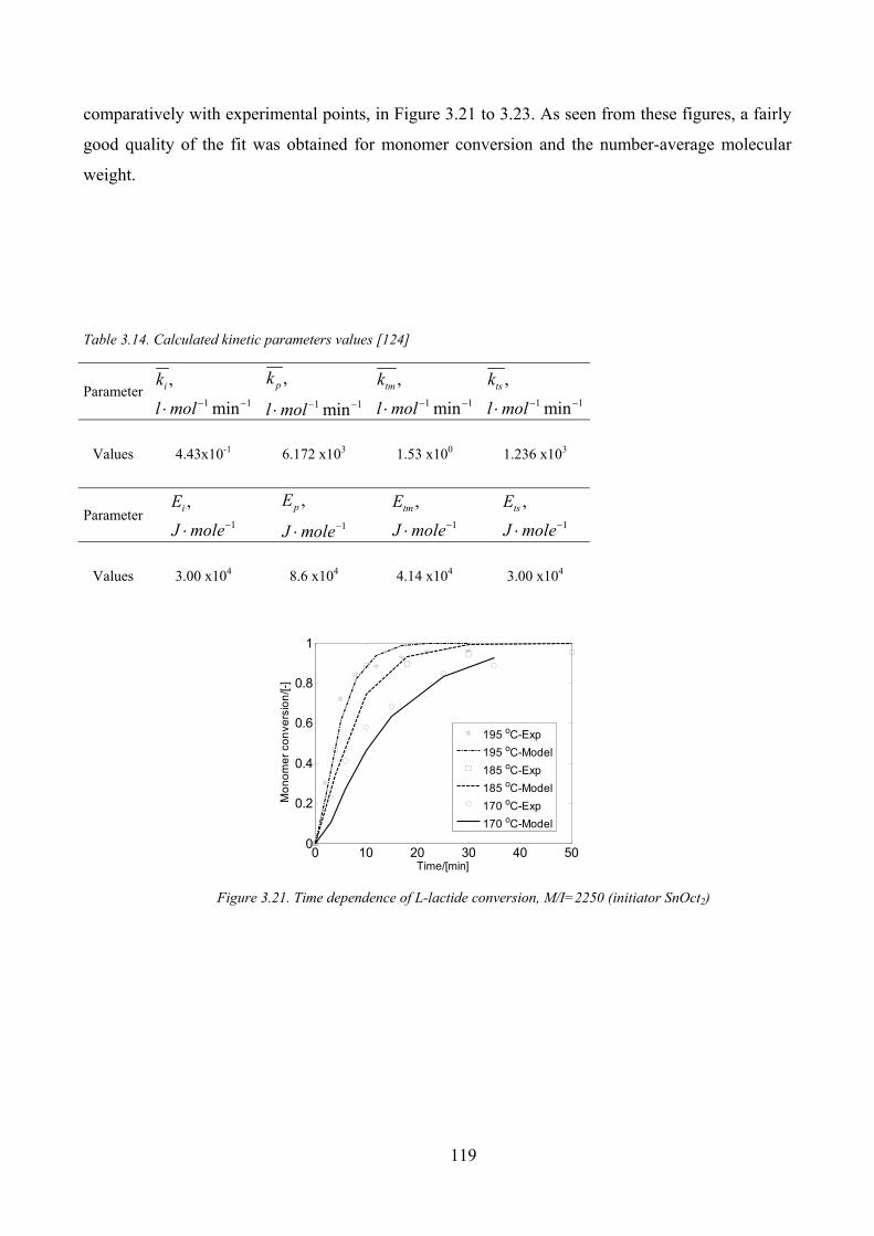
119
comparatively with experimental points, in Figure 3.21 to 3.23. As seen from these figures, a fairly
good quality of the fit was obtained for monomer conversion and the number-average molecular
weight.
Table 3.14. Calculated kinetic parameters values [124]
Parameter 1 1
,
min
ik
l mol− −⋅ 1 1
,
min
pk
l mol− −⋅ 1 1
,
min
tmk
l mol− −⋅ 1 1
,
min
tsk
l mol− −⋅Values 4.43x10⁻¹ 6.172 x10³ 1.53 x100 1.236 x10³
Parameter 1
,iE
J mole−⋅ 1
,pE
J mole−⋅ 1
,tmE
J mole−⋅ 1
,tsE
J mole−⋅
Values 3.00 x10⁴ 8.6 x10⁴ 4.14 x10⁴ 3.00 x10⁴
0 10 20 30 40 500
0.2
0.4
0.6
0.8
1
Time/[min]
Mo
no
me
r co
nve
rsio
n/[-]
195 oC-Exp
195 oC-Model
185 oC-Exp
185 oC-Model
170 oC-Exp
170 oC-Model
Figure 3.21. Time dependence of L-lactide conversion, M/I=2250 (initiator SnOct2)
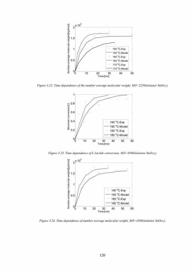
120
0 10 20 30 40 500
0.5
1
1.5
2x 10
4
Time/[min]
Nu
mb
er-
ave
rag
e m
ole
cu
lar
we
igh
t/[k
g/k
mo
l]
195 oC-Exp
195 oC-Model
185 oC-Exp
185 oC-Model
170 oC-Exp
170 oC-Model
Figure 3.22. Time dependence of the number average molecular weight, M/I=2250(initiator SnOct2)
0 10 20 30 40 50 600
0.2
0.4
0.6
0.8
1
Time/[min]
Mo
no
me
r co
nve
rsio
n/[-]
195 oC-Exp
195 oC-Model
185 oC-Exp
185 oC-Model
Figure 3.23. Time dependence of L-lactide conversion, M/I=4500(initiator SnOct2)
0 10 20 30 40 50 600
0.5
1
1.5
2x 10
4
Time/[min]
Nu
mb
er-
ave
rag
e m
ole
cu
lar
we
igh
t/[k
g/k
mo
l]
195 oC-Exp
195 oC-Model
185 oC-Exp
185 oC-Model
Figure 3.24. Time dependence of number average molecular weight, M/I=4500(initiator SnOct2)
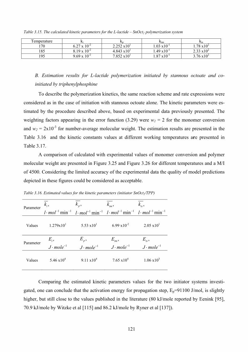
121
Table 3.15. The calculated kinetic parameters for the L-lactide – SnOct2 polymerization system
Temperature ki kp ktm kts 170 6.27 x 10⁻² 2.252 x101 1.03 x10⁻¹ 1.78 x10² 185 8.19 x 10⁻² 4.843 x101 1.49 x10⁻¹ 2.33 x10² 195 9.69 x 10⁻² 7.852 x101 1.87 x10⁻¹ 3.76 x10²
B. Estimation results for L-lactide polymerization initiated by stannous octoate and co-
initiated by triphenylphosphine
To describe the polymerization kinetics, the same reaction scheme and rate expressions were
considered as in the case of initiation with stannous octoate alone. The kinetic parameters were es-
timated by the procedure described above, based on experimental data previously presented. The
weighting factors appearing in the error function (3.29) were w1 = 2 for the monomer conversion
and w2 = 2x10⁻³ for number-average molecular weight. The estimation results are presented in the
Table 3.16 and the kinetic constants values at different working temperatures are presented in
Table 3.17.
A comparison of calculated with experimental values of monomer conversion and polymer
molecular weight are presented in Figure 3.25 and Figure 3.26 for different temperatures and a M/I
of 4500. Considering the limited accuracy of the experimental data the quality of model predictions
depicted in these figures could be considered as acceptable.
Table 3.16. Estimated values for the kinetic parameters (initiator SnOct2/TPP)
Parameter 1 1
,
min
ik
l mol− −⋅ 1 1
,
min
pk
l mol− −⋅ 1 1
,
min
tmk
l mol− −⋅ 1 1
,
min
tsk
l mol− −⋅Values 1.279x101 5.53 x101 6.99 x10⁻² 2.05 x101
Parameter 1
,iE
J mole−⋅ 1
,pE
J mole−⋅ 1
,tmE
J mole−⋅ 1
,tsE
J mole−⋅
Values 5.46 x10⁴ 9.11 x10⁴ 7.65 x10⁴ 1.06 x10⁵
Comparing the estimated kinetic parameters values for the two initiator systems investi-
gated, one can conclude that the activation energy for propagation step, Ep=91100 J/mol, is slightly
higher, but still close to the values published in the literature (80 kJ/mole reported by Eenink [95],
70.9 kJ/mole by Witzke et al [115] and 86.2 kJ/mole by Ryner et al [137]).
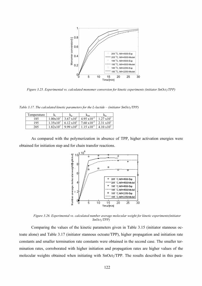
122
0 5 10 15 20 25 300
0.2
0.4
0.6
0.8
1
Time/[min]
Mo
no
me
r co
nve
rsio
n/[-]
205 oC, M/I=4500-Exp
205 oC, M/I=4500-Model
195 oC, M/I=4500-Exp
195 oC, M/I=4500-Model
185 oC, M/I=2250-Exp
185 oC, M/I=2250-Model
Figure 3.25. Experimental vs. calculated monomer conversion for kinetic experiments (initiator SnOct2/TPP)
Table 3.17. The calculated kinetic parameters for the L-lactide – (initiator SnOct2/TPP)
Temperature ki kp ktm kts 185 1.00x101 3.67 x101 4.95 x10⁻² 1.27 x101 195 1.35x101 6.12 x101 7.60 x10⁻² 2.31 x101 205 1.82x101 9.99 x10² 1.15 x10⁻¹ 4.10 x101
As compared with the polymerization in absence of TPP, higher activation energies were
obtained for initiation step and for chain transfer reactions.
Figure 3.26. Experimental vs. calculated number average molecular weight for kinetic experiments(initiator
SnOct2/TPP)
Comparing the values of the kinetic parameters given in Table 3.15 (initiator stannous oc-
toate alone) and Table 3.17 (initiator stannous octoate/TPP), higher propagation and initiation rate
constants and smaller termination rate constants were obtained in the second case. The smaller ter-
mination rates, corroborated with higher initiation and propagation rates are higher values of the
molecular weights obtained when initiating with SnOct2/TPP. The results described in this para-
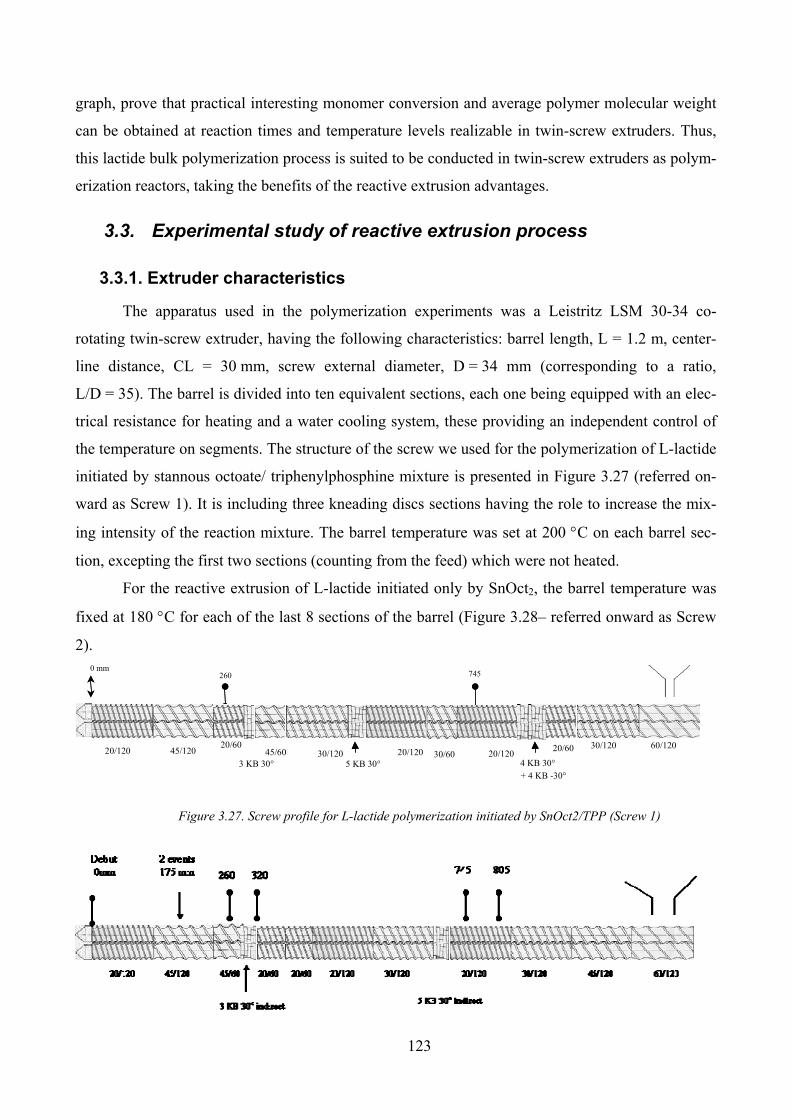
123
graph, prove that practical interesting monomer conversion and average polymer molecular weight
can be obtained at reaction times and temperature levels realizable in twin-screw extruders. Thus,
this lactide bulk polymerization process is suited to be conducted in twin-screw extruders as polym-
erization reactors, taking the benefits of the reactive extrusion advantages.
3.3. Experimental study of reactive extrusion process
3.3.1. Extruder characteristics
The apparatus used in the polymerization experiments was a Leistritz LSM 30-34 co-
rotating twin-screw extruder, having the following characteristics: barrel length, L = 1.2 m, center-
line distance, CL = 30 mm, screw external diameter, D = 34 mm (corresponding to a ratio,
L/D = 35). The barrel is divided into ten equivalent sections, each one being equipped with an elec-
trical resistance for heating and a water cooling system, these providing an independent control of
the temperature on segments. The structure of the screw we used for the polymerization of L-lactide
initiated by stannous octoate/ triphenylphosphine mixture is presented in Figure 3.27 (referred on-
ward as Screw 1). It is including three kneading discs sections having the role to increase the mix-
ing intensity of the reaction mixture. The barrel temperature was set at 200 °C on each barrel sec-
tion, excepting the first two sections (counting from the feed) which were not heated.
For the reactive extrusion of L-lactide initiated only by SnOct2, the barrel temperature was
fixed at 180 °C for each of the last 8 sections of the barrel (Figure 3.28– referred onward as Screw
2).
5 KB 30°
60/12030/12030/12020/120 45/120 20/120
0 mm
45/60 20/6020/12030/60
20/60
3 KB 30° 4 KB 30°
260 745
+ 4 KB -30°
Figure 3.27. Screw profile for L-lactide polymerization initiated by SnOct2/TPP (Screw 1)
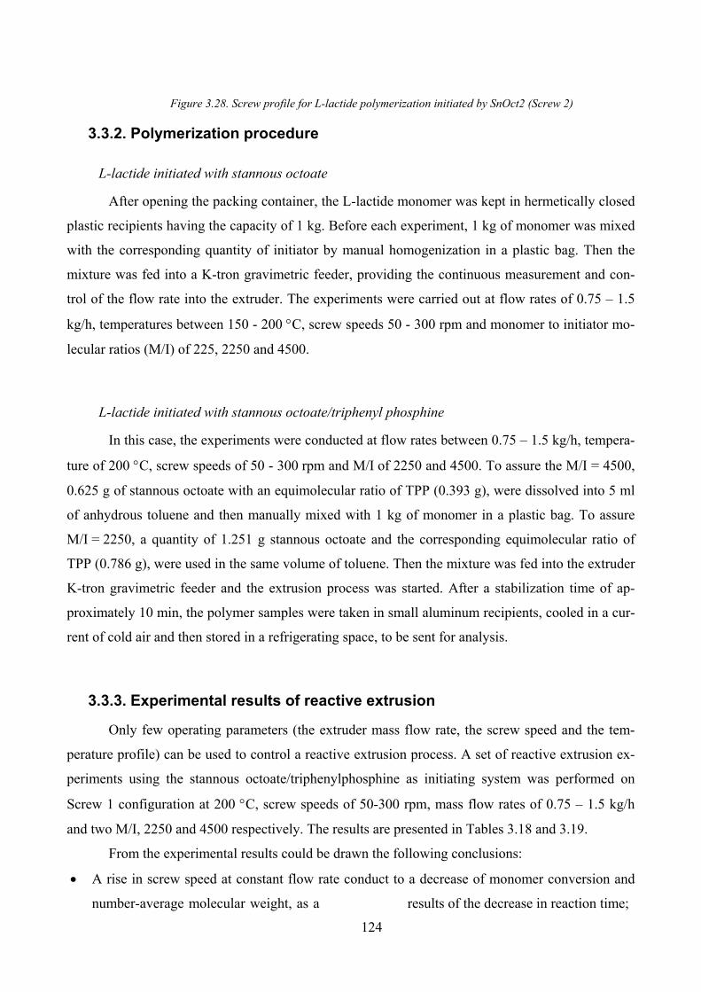
124
Figure 3.28. Screw profile for L-lactide polymerization initiated by SnOct2 (Screw 2)
3.3.2. Polymerization procedure
L-lactide initiated with stannous octoate
After opening the packing container, the L-lactide monomer was kept in hermetically closed
plastic recipients having the capacity of 1 kg. Before each experiment, 1 kg of monomer was mixed
with the corresponding quantity of initiator by manual homogenization in a plastic bag. Then the
mixture was fed into a K-tron gravimetric feeder, providing the continuous measurement and con-
trol of the flow rate into the extruder. The experiments were carried out at flow rates of 0.75 – 1.5
kg/h, temperatures between 150 - 200 °C, screw speeds 50 - 300 rpm and monomer to initiator mo-
lecular ratios (M/I) of 225, 2250 and 4500.
L-lactide initiated with stannous octoate/triphenyl phosphine
In this case, the experiments were conducted at flow rates between 0.75 – 1.5 kg/h, tempera-
ture of 200 °C, screw speeds of 50 - 300 rpm and M/I of 2250 and 4500. To assure the M/I = 4500,
0.625 g of stannous octoate with an equimolecular ratio of TPP (0.393 g), were dissolved into 5 ml
of anhydrous toluene and then manually mixed with 1 kg of monomer in a plastic bag. To assure
M/I = 2250, a quantity of 1.251 g stannous octoate and the corresponding equimolecular ratio of
TPP (0.786 g), were used in the same volume of toluene. Then the mixture was fed into the extruder
K-tron gravimetric feeder and the extrusion process was started. After a stabilization time of ap-
proximately 10 min, the polymer samples were taken in small aluminum recipients, cooled in a cur-
rent of cold air and then stored in a refrigerating space, to be sent for analysis.
3.3.3. Experimental results of reactive extrusion
Only few operating parameters (the extruder mass flow rate, the screw speed and the tem-
perature profile) can be used to control a reactive extrusion process. A set of reactive extrusion ex-
periments using the stannous octoate/triphenylphosphine as initiating system was performed on
Screw 1 configuration at 200 °C, screw speeds of 50-300 rpm, mass flow rates of 0.75 – 1.5 kg/h
and two M/I, 2250 and 4500 respectively. The results are presented in Tables 3.18 and 3.19.
From the experimental results could be drawn the following conclusions:
• A rise in screw speed at constant flow rate conduct to a decrease of monomer conversion and
number-average molecular weight, as a results of the decrease in reaction time;
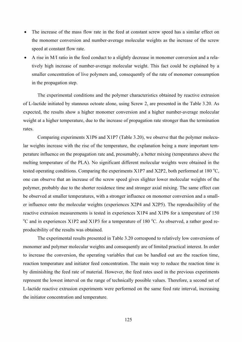
125
• The increase of the mass flow rate in the feed at constant screw speed has a similar effect on
the monomer conversion and number-average molecular weights as the increase of the screw
speed at constant flow rate.
• A rise in M/I ratio in the feed conduct to a slightly decrease in monomer conversion and a rela-
tively high increase of number-average molecular weight. This fact could be explained by a
smaller concentration of live polymers and, consequently of the rate of monomer consumption
in the propagation step.
The experimental conditions and the polymer characteristics obtained by reactive extrusion
of L-lactide initiated by stannous octoate alone, using Screw 2, are presented in the Table 3.20. As
expected, the results show a higher monomer conversion and a higher number-average molecular
weight at a higher temperature, due to the increase of propagation rate stronger than the termination
rates.
Comparing experiments X1P6 and X1P7 (Table 3.20), we observe that the polymer molecu-
lar weights increase with the rise of the temperature, the explanation being a more important tem-
perature influence on the propagation rate and, presumably, a better mixing (temperatures above the
melting temperature of the PLA). No significant different molecular weights were obtained in the
tested operating conditions. Comparing the experiments X1P7 and X2P2, both performed at 180 oC,
one can observe that an increase of the screw speed gives slighter lower molecular weights of the
polymer, probably due to the shorter residence time and stronger axial mixing. The same effect can
be observed at smaller temperatures, with a stronger influence on monomer conversion and a small-
er influence onto the molecular weights (experiences X2P4 and X2P5). The reproducibility of the
reactive extrusion measurements is tested in experiences X1P4 and X1P6 for a temperature of 150 oC and in experiences X1P2 and X1P3 for a temperature of 180 oC. As observed, a rather good re-
producibility of the results was obtained.
The experimental results presented in Table 3.20 correspond to relatively low conversions of
monomer and polymer molecular weights and consequently are of limited practical interest. In order
to increase the conversion, the operating variables that can be handled out are the reaction time,
reaction temperature and initiator feed concentration. The main way to reduce the reaction time is
by diminishing the feed rate of material. However, the feed rates used in the previous experiments
represent the lowest interval on the range of technically possible values. Therefore, a second set of
L-lactide reactive extrusion experiments were performed on the same feed rate interval, increasing
the initiator concentration and temperature.

126
Table 3.18. Reactive extrusion results at 200 °C and M/I = 2250 on Screw 1 (initiator SnOct2/TPP)
Experience iden-tificator
Rotation speed, [rot/min]
Mass flow rate, [kg/h]Monomer conversion,
[-] Mn,[kg/kmole] IP
1 50 0.75 0.91 70000 2.4
2 200 0.75 0.82 63000 2.5
3 300 0.75 0.80 62000 2.7
4 50 1.25 0.87 65000 2.7
5 200 1.25 0.74 64000 2.4
6 300 1.25 0.68 60000 2.3
7 50 1.5 0.72 61000 1.9
8 200 1.5 0.65 59000 2.1
9 300 1.5 0.52 57000 2.3
Table 3.19. Reactive extrusion results at 200 °C and M/I = 4500 on Screw 1(initiator SnOct2/TPP)
Experience iden-tificator
Rotation speed, [rot/min]
Mass flow rate, [kg/h]Monomer conversion,
[-] Mn,[kg/kmole] IP
1 50 0.75 0.80 95000 2.3
2 200 0.75 0.75 90000 2.3
3 300 0.75 0.70 72000 1.6
4 50 1.25 0.73 81000 1.9
5 200 1.25 0.65 73000 2.4
6 300 1.25 0.60 60000 1.6
7 50 1.5 0.70 75000 2.4
8 200 1.5 0.50 67000 1.9
9 300 1.5 0.47 55000 1.8
The operating conditions and process performances are given in Table 3.21. As observed,
higher lactide conversion values are obtained and slightly superior molecular weights of polymer
(mainly as consequence of temperature increase. In spite of some advantages regarding the mono-
mer conversion and polymer molecular weights, the relatively high content of stannous compounds
is an important drawback of the process conducted in these operating conditions.
For a low M/I ratio, practically the same monomer conversion is obtained for all operating
conditions presented in Table 3.21. This fact could be explained by higher initiation and conse-
quently higher propagation rates, due to the higher initiator concentration that produces very fast
monomer consumption in short polymerization times. At constant flow rate, higher molecular
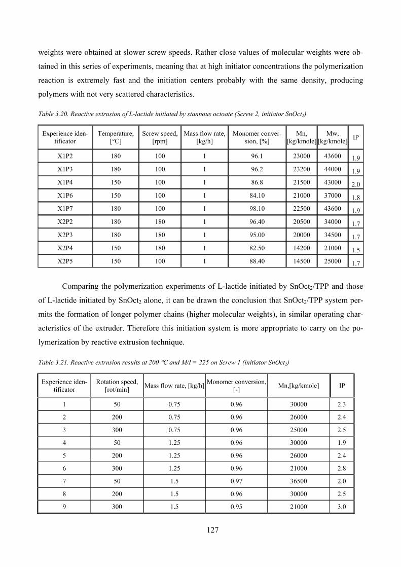
127
weights were obtained at slower screw speeds. Rather close values of molecular weights were ob-
tained in this series of experiments, meaning that at high initiator concentrations the polymerization
reaction is extremely fast and the initiation centers probably with the same density, producing
polymers with not very scattered characteristics.
Table 3.20. Reactive extrusion of L-lactide initiated by stannous octoate (Screw 2, initiator SnOct2)
Experience iden-tificator
Temperature, [°C]
Screw speed, [rpm]
Mass flow rate, [kg/h]
Monomer conver-sion, [%]
Mn, [kg/kmole]
Mw, [kg/kmole]
IP
X1P2 180 100 1 96.1 23000 43600 1.9
X1P3 180 100 1 96.2 23200 44000 1.9
X1P4 150 100 1 86.8 21500 43000 2.0
X1P6 150 100 1 84.10 21000 37000 1.8
X1P7 180 100 1 98.10 22500 43600 1.9
X2P2 180 180 1 96.40 20500 34000 1.7
X2P3 180 180 1 95.00 20000 34500 1.7
X2P4 150 180 1 82.50 14200 21000 1.5
X2P5 150 100 1 88.40 14500 25000 1.7
Comparing the polymerization experiments of L-lactide initiated by SnOct2/TPP and those
of L-lactide initiated by SnOct2 alone, it can be drawn the conclusion that SnOct2/TPP system per-
mits the formation of longer polymer chains (higher molecular weights), in similar operating char-
acteristics of the extruder. Therefore this initiation system is more appropriate to carry on the po-
lymerization by reactive extrusion technique.
Table 3.21. Reactive extrusion results at 200 °C and M/I = 225 on Screw 1 (initiator SnOct2)
Experience iden-tificator
Rotation speed, [rot/min]
Mass flow rate, [kg/h]Monomer conversion,
[-] Mn,[kg/kmole] IP
1 50 0.75 0.96 30000 2.3
2 200 0.75 0.96 26000 2.4
3 300 0.75 0.96 25000 2.5
4 50 1.25 0.96 30000 1.9
5 200 1.25 0.96 26000 2.4
6 300 1.25 0.96 21000 2.8
7 50 1.5 0.97 36500 2.0
8 200 1.5 0.96 30000 2.5
9 300 1.5 0.95 21000 3.0
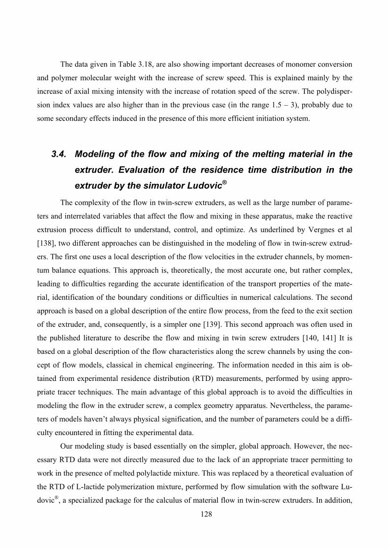
128
The data given in Table 3.18, are also showing important decreases of monomer conversion
and polymer molecular weight with the increase of screw speed. This is explained mainly by the
increase of axial mixing intensity with the increase of rotation speed of the screw. The polydisper-
sion index values are also higher than in the previous case (in the range 1.5 – 3), probably due to
some secondary effects induced in the presence of this more efficient initiation system.
3.4. Modeling of the flow and mixing of the melting material in the
extruder. Evaluation of the residence time distribution in the
extruder by the simulator Ludovic®
The complexity of the flow in twin-screw extruders, as well as the large number of parame-
ters and interrelated variables that affect the flow and mixing in these apparatus, make the reactive
extrusion process difficult to understand, control, and optimize. As underlined by Vergnes et al
[138], two different approaches can be distinguished in the modeling of flow in twin-screw extrud-
ers. The first one uses a local description of the flow velocities in the extruder channels, by momen-
tum balance equations. This approach is, theoretically, the most accurate one, but rather complex,
leading to difficulties regarding the accurate identification of the transport properties of the mate-
rial, identification of the boundary conditions or difficulties in numerical calculations. The second
approach is based on a global description of the entire flow process, from the feed to the exit section
of the extruder, and, consequently, is a simpler one [139]. This second approach was often used in
the published literature to describe the flow and mixing in twin screw extruders [140, 141] It is
based on a global description of the flow characteristics along the screw channels by using the con-
cept of flow models, classical in chemical engineering. The information needed in this aim is ob-
tained from experimental residence distribution (RTD) measurements, performed by using appro-
priate tracer techniques. The main advantage of this global approach is to avoid the difficulties in
modeling the flow in the extruder screw, a complex geometry apparatus. Nevertheless, the parame-
ters of models haven’t always physical signification, and the number of parameters could be a diffi-
culty encountered in fitting the experimental data.
Our modeling study is based essentially on the simpler, global approach. However, the nec-
essary RTD data were not directly measured due to the lack of an appropriate tracer permitting to
work in the presence of melted polylactide mixture. This was replaced by a theoretical evaluation of
the RTD of L-lactide polymerization mixture, performed by flow simulation with the software Lu-
dovic®, a specialized package for the calculus of material flow in twin-screw extruders. In addition,
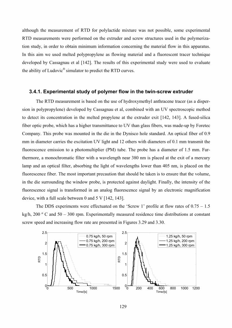
129
although the measurement of RTD for polylactide mixture was not possible, some experimental
RTD measurements were performed on the extruder and screw structures used in the polymeriza-
tion study, in order to obtain minimum information concerning the material flow in this apparatus.
In this aim we used melted polypropylene as flowing material and a fluorescent tracer technique
developed by Cassagnau et al [142]. The results of this experimental study were used to evaluate
the ability of Ludovic® simulator to predict the RTD curves.
3.4.1. Experimental study of polymer flow in the twin-screw extruder
The RTD measurement is based on the use of hydroxymethyl anthracene tracer (as a disper-
sion in polypropylene) developed by Cassagnau et al, combined with an UV spectroscopic method
to detect its concentration in the melted propylene at the extruder exit [142, 143]. A fused-silica
fiber optic probe, which has a higher transmittance to UV than glass fibers, was made-up by Foretec
Company. This probe was mounted in the die in the Dynisco hole standard. An optical fiber of 0.9
mm in diameter carries the excitation UV light and 12 others with diameters of 0.1 mm transmit the
fluorescence emission to a photomultiplier (PM) tube. The probe has a diameter of 1.5 mm. Fur-
thermore, a monochromatic filter with a wavelength near 380 nm is placed at the exit of a mercury
lamp and an optical filter, absorbing the light of wavelengths lower than 405 nm, is placed on the
fluorescence fiber. The most important precaution that should be taken is to ensure that the volume,
in the die surrounding the window probe, is protected against daylight. Finally, the intensity of the
fluorescence signal is transformed in an analog fluorescence signal by an electronic magnification
device, with a full scale between 0 and 5 V [142, 143].
The DDS experiments were effectuated on the ‘Screw 1’ profile at flow rates of 0.75 – 1.5
kg/h, 200 º C and 50 – 300 rpm. Experimentally measured residence time distributions at constant
screw speed and increasing flow rate are presented in Figures 3.29 and 3.30.
0 500 1000 1500
0
0.5
1
1.5
2
2.5
Time/[s]
RT
D
0.75 kg/h, 50 rpm
0.75 kg/h, 200 rpm
0.75 kg/h, 300 rpm
0 200 400 600 800 1000 12000
0.5
1
1.5
2
2.5
Time/[s]
RT
D
1.25 kg/h, 50 rpm
1.25 kg/h, 200 rpm
1.25 kg/h, 300 rpm
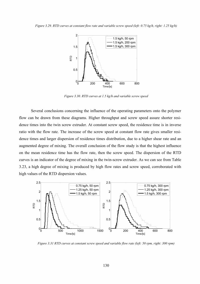
130
Figure 3.29. RTD curves at constant flow rate and variable screw speed (left: 0.75 kg/h, right: 1.25 kg/h)
0 200 400 600 8000
0.5
1
1.5
2
Time/[s]
RT
D
1.5 kg/h, 50 rpm
1.5 kg/h, 200 rpm
1.5 kg/h, 300 rpm
Figure 3.30. RTD curves at 1.5 kg/h and variable screw speed
Several conclusions concerning the influence of the operating parameters onto the polymer
flow can be drawn from these diagrams. Higher throughput and screw speed assure shorter resi-
dence times into the twin screw extruder. At constant screw speed, the residence time is in inverse
ratio with the flow rate. The increase of the screw speed at constant flow rate gives smaller resi-
dence times and larger dispersion of residence times distribution, due to a higher shear rate and an
augmented degree of mixing. The overall conclusion of the flow study is that the highest influence
on the mean residence time has the flow rate, then the screw speed. The dispersion of the RTD
curves is an indicator of the degree of mixing in the twin-screw extruder. As we can see from Table
3.23, a high degree of mixing is produced by high flow rates and screw speed, corroborated with
high values of the RTD dispersion values.
Figure 3.31 RTD curves at constant screw speed and variable flow rate (left: 50 rpm, right: 300 rpm)
0 500 1000 15000
0.5
1
1.5
2
2.5
Time/[s]
RT
D
0.75 kg/h, 50 rpm
1.25 kg/h, 50 rpm
1.5 kg/h, 50 rpm
0 200 400 600 8000
0.5
1
1.5
2
2.5
Time/[s]
RT
D
0.75 kg/h, 300 rpm
1.25 kg/h, 300 rpm
1.5 kg/h, 300 rpm
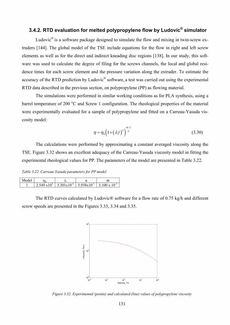
131
3.4.2. RTD evaluation for melted polypropylene flow by Ludovic® simulator
Ludovic® is a software package designed to simulate the flow and mixing in twin-screw ex-
truders [144]. The global model of the TSE include equations for the flow in right and left screw
elements as well as for the direct and indirect kneading disc regions [138]. In our study, this soft-
ware was used to calculate the degree of filing for the screws channels, the local and global resi-
dence times for each screw element and the pressure variation along the extruder. To estimate the
accuracy of the RTD prediction by Ludovic® software, a test was carried out using the experimental
RTD data described in the previous section, on polypropylene (PP) as flowing material.
The simulations were performed in similar working conditions as for PLA synthesis, using a
barrel temperature of 200 oC and Screw 1 configuration. The rheological properties of the material
were experimentally evaluated for a sample of polypropylene and fitted on a Carreau-Yasuda vis-
cosity model:
( )( ) 1
0 1m
a aη η λγ −= + & (3.30)
The calculations were performed by approximating a constant averaged viscosity along the
TSE. Figure 3.32 shows an excellent adequacy of the Carreau-Yasuda viscosity model in fitting the
experimental rheological values for PP. The parameters of the model are presented in Table 3.22.
Table 3.22. Carreau-Yasuda parameters for PP model
Model η0 λ a m 1 2.549 x10³ 3.301x10⁻¹ 5.938x10⁻¹ 5.100 x 10⁻¹
The RTD curves calculated by Ludovic® software for a flow rate of 0.75 kg/h and different
screw speeds are presented in the Figures 3.33, 3.34 and 3.35.
10-2
10-1
100
101
102
102
103
104
Gamma, 1/s
Vis
cosity,
Pa s
Figure 3.32. Experimental (points) and calculated (line) values of polypropylene viscosity
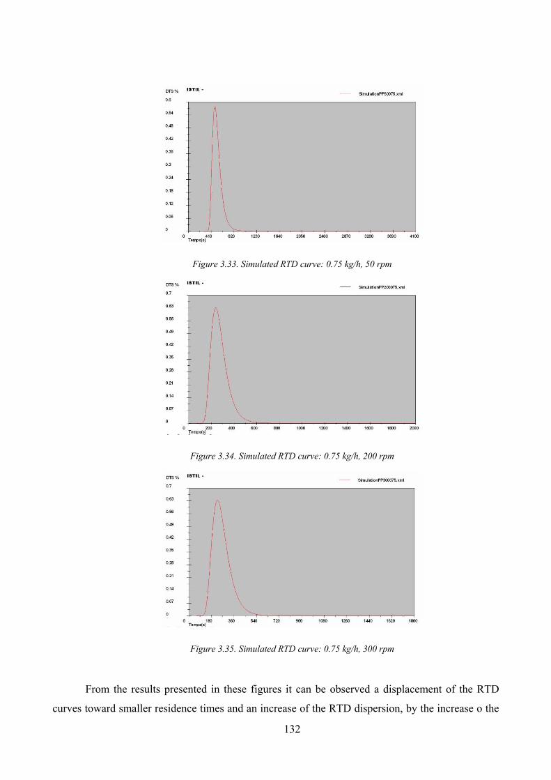
132
Figure 3.33. Simulated RTD curve: 0.75 kg/h, 50 rpm
Figure 3.34. Simulated RTD curve: 0.75 kg/h, 200 rpm
Figure 3.35. Simulated RTD curve: 0.75 kg/h, 300 rpm
From the results presented in these figures it can be observed a displacement of the RTD
curves toward smaller residence times and an increase of the RTD dispersion, by the increase o the
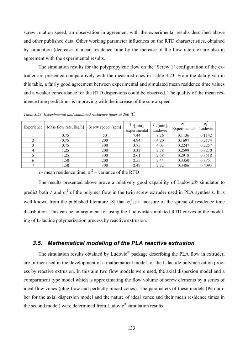
133
screw rotation speed, an observation in agreement with the experimental results described above
and other published data. Other working parameter influences on the RTD characteristics, obtained
by simulation (decrease of mean residence time by the increase of the flow rate etc) are also in
agreement with the experimental results.
The simulation results for the polypropylene flow on the ‘Screw 1’ configuration of the ex-
truder are presented comparatively with the measured ones in Table 3.23. From the data given in
this table, a fairly good agreement between experimental and simulated mean residence time values
and a weaker concordance for the RTD dispersions could be observed. The quality of the mean res-
idence time predictions is improving with the increase of the screw speed.
Table 3.23. Experimental and simulated residence times at 200 ºC
Experience Mass flow rate, [kg/h] Screw speed, [rpm] t /[min],
Experimental
t /[min], Ludovic
σt2
Experimental σt
2
Ludovic
1 0.75 50 7.44 8.26 0.1136 0.1142 2 0.75 200 4.94 4.20 0.1697 0.2174 3 0.75 300 3.75 4.03 0.2247 0.2257 4 1.25 200 3.32 2.78 0.2599 0.3270 5 1.25 300 2.61 2.58 0.2918 0.3518 6 1.50 200 2.55 2.44 0.3350 0.3751 7 1.50 300 2.49 2.22 0.3486 0.4093
t - mean residence time, σt2 – variance of the RTD
The results presented above prove a relatively good capability of Ludovic® simulator to
predict both t and σt2 of the polymer flow in the twin screw extruder used in PLA synthesis. It is
well known from the published literature [8] that 2tσ is a measure of the spread of residence time
distribution. This can be an argument for using the Ludovic® simulated RTD curves in the model-
ing of L-lactide polymerization process by reactive extrusion.
3.5. Mathematical modeling of the PLA reactive extrusion
The simulation results obtained by Ludovic® package describing the PLA flow in extruder,
are further used in the development of a mathematical model for the L-lactide polymerization proc-
ess by reactive extrusion. In this aim two flow models were used, the axial dispersion model and a
compartment type model which is approximating the flow volume of screw elements by a series of
ideal flow zones (plug flow and perfectly mixed zones). The parameters of these models (Pe num-
ber for the axial dispersion model and the nature of ideal zones and their mean residence times in
the second model) were determined from Ludovic® simulation results.
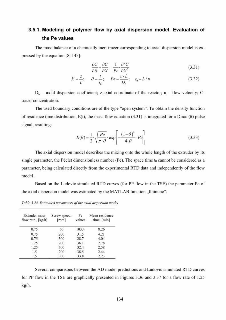
134
3.5.1. Modeling of polymer flow by axial dispersion model. Evaluation of
the Pe values
The mass balance of a chemically inert tracer corresponding to axial dispersion model is ex-
pressed by the equation [8, 145]:
2
2
1C C C
X Pe Xθ∂ ∂ ∂+ = ⋅∂ ∂ ∂ (3.31)
00
; ; ; /L
z t u LX Pe t L u
L t Dθ ⋅= ⋅ = = = (3.32)
DL – axial dispersion coefficient; z-axial coordinate of the reactor; u – flow velocity; C-
tracer concentration.
The used boundary conditions are of the type “open system”. To obtain the density function
of residence time distribution, E(t), the mass flow equation (3.31) is integrated for a Dirac (δ) pulse
signal, resulting:
( )211
( ) exp2 4
PeE Pe
θθ π θ θ⎡ ⎤−= ⋅ ⋅ − ⋅⎢ ⎥⋅ ⋅⎢ ⎥⎣ ⎦ (3.33)
The axial dispersion model describes the mixing onto the whole length of the extruder by its
single parameter, the Péclet dimensionless number (Pe). The space time t0 cannot be considered as a
parameter, being calculated directly from the experimental RTD data and independently of the flow
model .
Based on the Ludovic simulated RTD curves (for PP flow in the TSE) the parameter Pe of
the axial dispersion model was estimated by the MATLAB function „fminunc”.
Table 3.24. Estimated parameters of the axial dispersion model
Extruder mass flow rate , [kg/h]
Screw speed, [rpm]
Pe values
Mean residence time, [min]
0.75 50 103.4 8.26 0.75 200 31.5 4.21 0.75 300 28.7 4.04 1.25 200 36.1 2.78 1.25 300 32.4 2.58 1.5 200 38.5 2.44 1.5 300 33.8 2.23
Several comparisons between the AD model predictions and Ludovic simulated RTD curves
for PP flow in the TSE are graphically presented in Figures 3.36 and 3.37 for a flow rate of 1.25
kg/h.
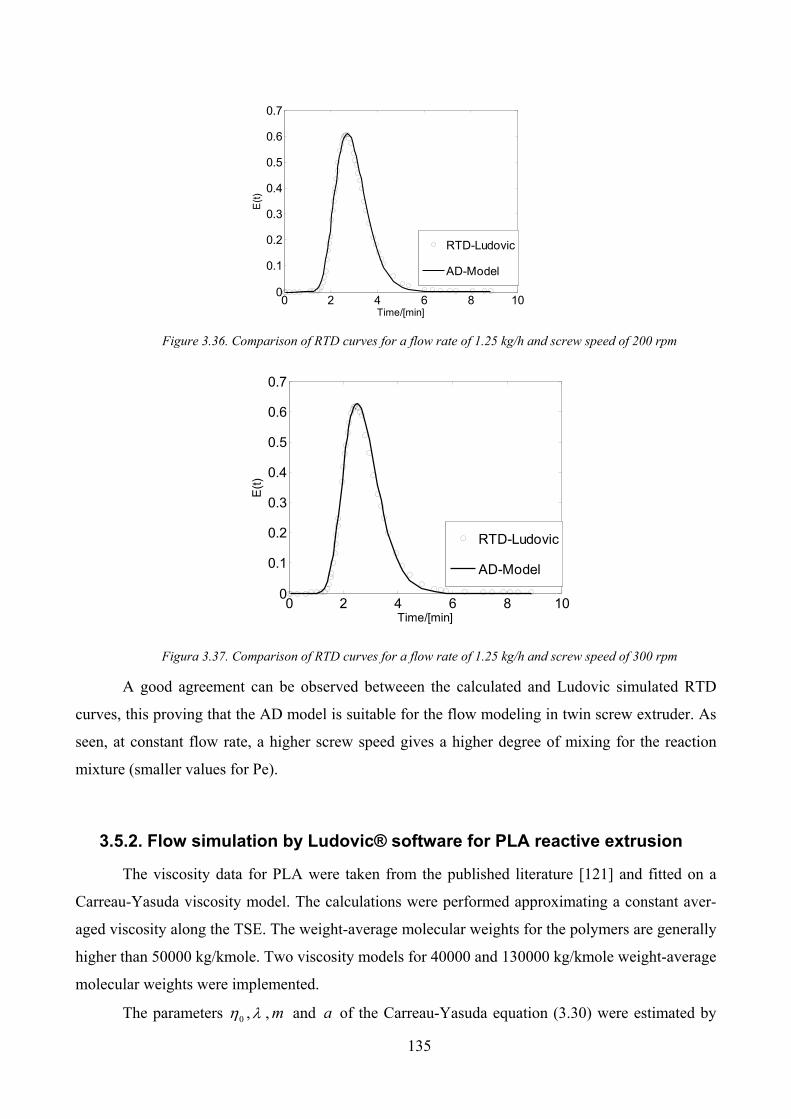
135
0 2 4 6 8 100
0.1
0.2
0.3
0.4
0.5
0.6
0.7
Time/[min]
E(t
)
RTD-Ludovic
AD-Model
Figure 3.36. Comparison of RTD curves for a flow rate of 1.25 kg/h and screw speed of 200 rpm
0 2 4 6 8 100
0.1
0.2
0.3
0.4
0.5
0.6
0.7
Time/[min]
E(t
)
RTD-Ludovic
AD-Model
Figura 3.37. Comparison of RTD curves for a flow rate of 1.25 kg/h and screw speed of 300 rpm
A good agreement can be observed betweeen the calculated and Ludovic simulated RTD
curves, this proving that the AD model is suitable for the flow modeling in twin screw extruder. As
seen, at constant flow rate, a higher screw speed gives a higher degree of mixing for the reaction
mixture (smaller values for Pe).
3.5.2. Flow simulation by Ludovic® software for PLA reactive extrusion
The viscosity data for PLA were taken from the published literature [121] and fitted on a
Carreau-Yasuda viscosity model. The calculations were performed approximating a constant aver-
aged viscosity along the TSE. The weight-average molecular weights for the polymers are generally
higher than 50000 kg/kmole. Two viscosity models for 40000 and 130000 kg/kmole weight-average
molecular weights were implemented.
The parameters 0η , λ , m and a of the Carreau-Yasuda equation (3.30) were estimated by

136
using the viscosity data published by Cooper-White and Mackay [121] . The calculated parameters
are given in Table 3.25 and a comparison between the predicted and published values of polymer
viscosity is presented in Figure 3.38.
Table 3.25. Estimated values for the parameters of the Carreau-Yasuda viscosity model
Model η0 λ a m Mw 1 1.029x10² 7.658x10⁻³ 2.018x100 7.711x 10⁻¹ 40000 2 7.118x10³ 1.133x 10⁻¹ 9.033x10⁻¹ 5.100x 10⁻¹ 130000 3 9.525x10⁵ 1.081x101 3.843x 10⁻¹ 3.582 x10⁻¹ 360000
10-3
10-2
10-1
100
101
102
103
101
102
103
104
105
106
Gamma, 1/s
Vis
cosity,
Pa s
Mw = 40000-exp
Mw = 40000-calc
Mw = 130000-exp
Mw = 130000-calc
Mw = 360000-exp
Mw = 360000-calc
Figure 3.38. Published [121] and calculated viscosity values at 200 oC
Several local and global residence times predicted by Ludovic® are presented in the follow-
ing figures for the screw profile in Figure 3.27 (Screw 1). A constant temperature of 200 oC was
considered along the extruder barrel, accordingly with the experimental operating conditions.
Figure 3.39. Residence time for the viscosity model 1
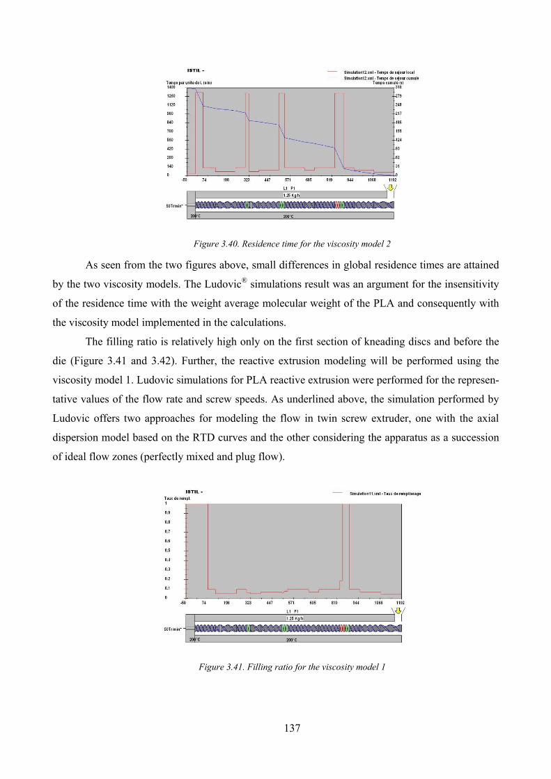
137
Figure 3.40. Residence time for the viscosity model 2
As seen from the two figures above, small differences in global residence times are attained
by the two viscosity models. The Ludovic® simulations result was an argument for the insensitivity
of the residence time with the weight average molecular weight of the PLA and consequently with
the viscosity model implemented in the calculations.
The filling ratio is relatively high only on the first section of kneading discs and before the
die (Figure 3.41 and 3.42). Further, the reactive extrusion modeling will be performed using the
viscosity model 1. Ludovic simulations for PLA reactive extrusion were performed for the represen-
tative values of the flow rate and screw speeds. As underlined above, the simulation performed by
Ludovic offers two approaches for modeling the flow in twin screw extruder, one with the axial
dispersion model based on the RTD curves and the other considering the apparatus as a succession
of ideal flow zones (perfectly mixed and plug flow).
Figure 3.41. Filling ratio for the viscosity model 1
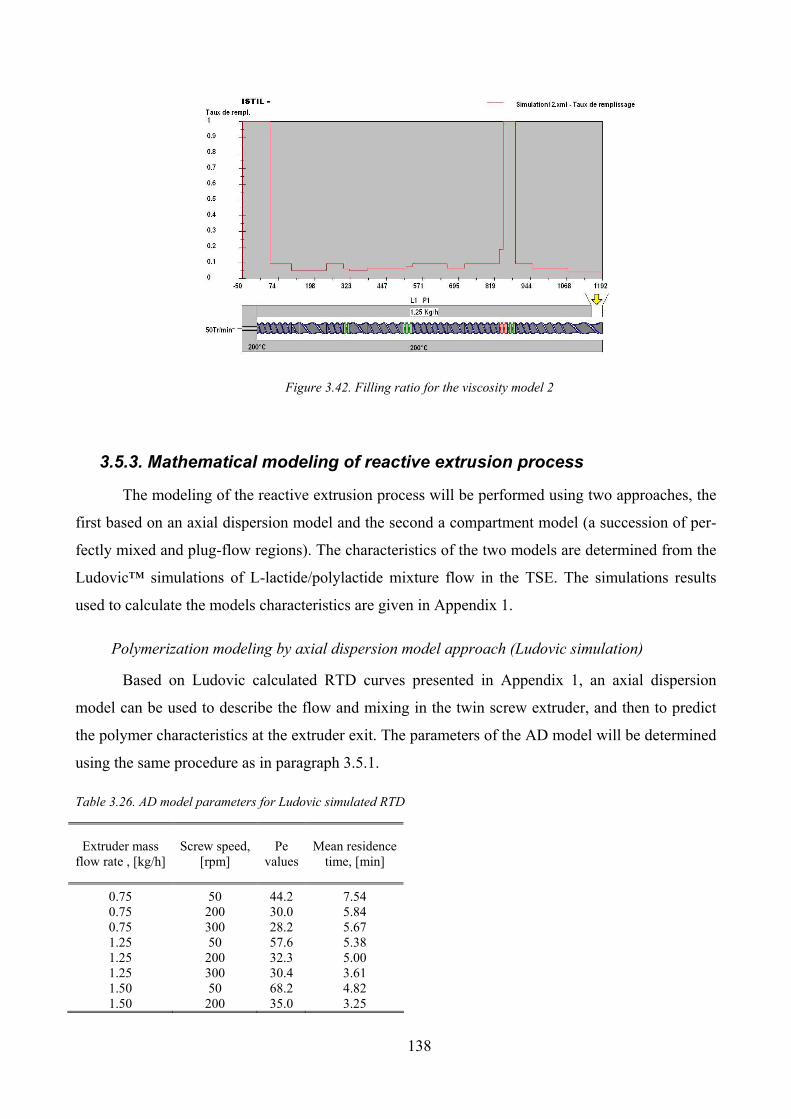
138
Figure 3.42. Filling ratio for the viscosity model 2
3.5.3. Mathematical modeling of reactive extrusion process
The modeling of the reactive extrusion process will be performed using two approaches, the
first based on an axial dispersion model and the second a compartment model (a succession of per-
fectly mixed and plug-flow regions). The characteristics of the two models are determined from the
Ludovic™ simulations of L-lactide/polylactide mixture flow in the TSE. The simulations results
used to calculate the models characteristics are given in Appendix 1.
Polymerization modeling by axial dispersion model approach (Ludovic simulation)
Based on Ludovic calculated RTD curves presented in Appendix 1, an axial dispersion
model can be used to describe the flow and mixing in the twin screw extruder, and then to predict
the polymer characteristics at the extruder exit. The parameters of the AD model will be determined
using the same procedure as in paragraph 3.5.1.
Table 3.26. AD model parameters for Ludovic simulated RTD
Extruder mass flow rate , [kg/h]
Screw speed, [rpm]
Pe values
Mean residence time, [min]
0.75 50 44.2 7.54 0.75 200 30.0 5.84 0.75 300 28.2 5.67 1.25 50 57.6 5.38 1.25 200 32.3 5.00 1.25 300 30.4 3.61 1.50 50 68.2 4.82 1.50 200 35.0 3.25

139
The mass balance equation for a chemical species, particular for the axial dispersion model,
has the form:
2
0 ,2
10R C
e
C Ct v
P X X
∂ ∂+ − =∂ ∂ (3.34)
With the boundary conditions:
0
10,
e
CX C C
P X
∂= − = − ∂ (3.35)
1, 0C
XX
∂= =∂ (3.36)
Where C stands for CM-monomer concentration, CI – initiator concentration, CS – impurities
concentration, 0th, 1st and 2nd order moment for radical ( λi, i=0..2) and polymers distribution con-
centrations (µi, i= 0..2); C0 – the value of C in the feed.
For the distribution moments, the boundary condition (3.35) becomes:
1
0,e
CX C
P X
∂= = ∂ (3.37)
The reaction rates for the chemical species in the mixture are:
,R I iv k IM= (3.38)
, 0 0R M i p tmv k IM k M k Mλ λ= + + (3.39)
0,R iv k IMλ = − (3.40)
( ) ( )( )1, 0 0 1 0 1R i p tm tsv k IM k M k M k Sλ λ λ λ λ λ= − + + − + − (3.41)
( ) ( )( )2, 1 0 0 2 0 22R i p p tm tsv k IM k M k M k M k Sλ λ λ λ λ λ λ= − + + + − + − (3.42)
( )0, 0 0R tm tsv k M k Sμ λ λ= − + (3.43)
( )1, 1 1R tm tsv k M k Sμ λ λ= − + (3.44)
( )2, 2 2R tm tsv k M k Sμ λ λ= − + (3.45)
, 0SR C tsv k Sλ= − (3.46)
The mathematical model was solved using a procedure based on the estimation function
„bvp4c” (MATLAB). This function solves the two-point boundary value conditions problems, as in
this case.
TSE extruder as a compartment model
The objective of this paragraph is to simulate the behavior of the twin screw extruder ap-
proximated as a compartment model (series of perfectly mixed and plug-flow zones) for all operat-
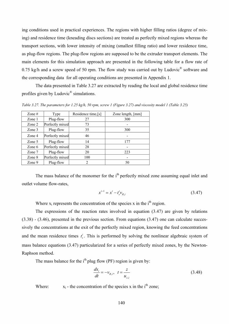
140
ing conditions used in practical experiences. The regions with higher filling ratios (degree of mix-
ing) and residence time (kneading discs sections) are treated as perfectly mixed regions whereas the
transport sections, with lower intensity of mixing (smallest filling ratio) and lower residence time,
as plug-flow regions. The plug-flow regions are supposed to be the extruder transport elements. The
main elements for this simulation approach are presented in the following table for a flow rate of
0.75 kg/h and a screw speed of 50 rpm. The flow study was carried out by Ludovic® software and
the corresponding data for all operating conditions are presented in Appendix 1.
The data presented in Table 3.27 are extracted by reading the local and global residence time
profiles given by Ludovic® simulations.
Table 3.27. The parameters for 1.25 kg/h, 50 rpm, screw 1 (Figure 3.27) and viscosity model 1 (Table 3.25)
Zone # Type Residence time,[s] Zone length, [mm] Zone 1 Plug-flow 27 300 Zone 2 Perfectly mixed 73 -
Zone 3 Plug-flow 35 300
Zone 4 Perfectly mixed 46 -
Zone 5 Plug-flow 14 177 Zone 6 Perfectly mixed 28 - Zone 7 Plug-flow 20 223 Zone 8 Perfectly mixed 100 - Zone 9 Plug-flow 2 50
The mass balance of the monomer for the ith perfectly mixed zone assuming equal inlet and
outlet volume flow-rates,
1,
i i i
s R ix x t v− = − (3.47)
Where xi represents the concentration of the species x in the ith region.
The expressions of the reaction rates involved in equation (3.47) are given by relations
(3.38) - (3.46), presented in the previous section. From equations (3.47) one can calculate succes-
sively the concentrations at the exit of the perfectly mixed region, knowing the feed concentrations
and the mean residence times i
st . This is performed by solving the nonlinear algebraic system of
mass balance equations (3.47) particularized for a series of perfectly mixed zones, by the Newton-
Raphson method.
The mass balance for the ith plug flow (PF) region is given by:
,,
,iR i
z i
dx zv t
dt u= − = (3.48)
Where: xi - the concentration of the species x in the ith zone;

141
,z iu - the flow speed in the ith zone;
,R iv - the consumption rate of the xi species;
The integration of the PF model was performed with a procedure based on a Runge-Kutta
fifth order algorithm implemented in MATLAB® programming package. An example of simulation
will be made for a mass flow-rate of 1.25 kg/h, a screw speed of 50 rpm, using the results obtained
for first viscosity model. Using the flow parameters specified in Table 3.27 the kinetic constants
presented in paragraph 3.2.4, the behavior of the reactive extrusion process was simulated. The re-
sults in terms of monomer conversion and number-average molecular weights profiles are presented
in Figure 3.43.
A monomer conversion of 0.81 and a number-average molecular weight of 71000 kg/kmole
are obtained at the extruder exit.
The characteristics of the compartment model for all operating conditions are presented in
Appendix 1. The comparison of the two modeling approaches in terms of monomer conversion and
number-average molecular weights profiles along the extruder will be presented in Figures 3.45 –
3.51. A comparison with the experimental results is shown in Tables 3.28 and 3.29.
Figure 3.43.Simulated chemical transformation for a M/I of 2250(initiator SnOct2/TFF, flow rate 1.25 kg/h,
screw speed 50 rpm)
Comparison of simulation results predicted by the two modeling approaches
A global comparison of monomer conversions and number-average molecular weights pro-
files predicted by both approaches is performed in this paragraph. A flow rate of 0.75 kg/h and a
screw speed of 50 rpm are used to simulate the twin-screw extruder, for both M/I ratios, and the
results are graphically presented in Figure 3.44. From the diagrams presented in this figure it can be
0 1 2 3 4 5 60
0.2
0.4
0.6
0.8
1
Time/[min]
Mo
no
me
r co
nve
rsio
n/[-]
1.25 kg/h, 50 rpm
0 1 2 3 4 5 60
2
4
6
8x 10
4
Time/[min]
Nu
mb
er-
ave
rag
e m
ole
cu
lar
we
igh
t/[k
g/k
mo
l]
1.25 kg/h, 50 rpm

142
observed that the two models predict practically the same values at the extruder exit for both mo-
nomer conversion and number-average molecular weights.
The difference between the approaches consists only in mathematical implementation. The
compartment model is simpler to implement, due to a simpler form of the mass balance equations,
usually not involving convergence problems in calculating the solution.
Figure 3.44. Twin screw extruder simulation by the two modeling approaches (DA Model – axial dispersion
model, Compart Model – Compartment model)
By comparison, the AD model stands for solving a two point boundary values problem,
which could sometimes have convergence problems. Also higher calculation time is required to the
simulations by AD model. The conclusion that can be draw is that, in the modeling of the reactive
extrusion process can be further used the mathematical model for which we have all parameters.
Nevertheless, the structure of the compartment model formulated in these calculations is less rigor-
ously formulated as compared with the DA model.
In what follows, a simulation of the PLA polymerization process will be performed using
the AD model, based on the Ludovic® simulated RTD data, with its parameters given in Table 3.24
and the kinetic model developed in the paragraph 3.2. An example of the simulated monomer con-
version and number-average molecular weight profiles for a flow rate of 0.75 kg/h and screw speeds
of 200 and 300 rpm are graphically presented in Figures 3.45 and 3.46. A comparison of the simu-
lated results with the experimental data for all operating conditions is presented in Tables 3.28 and
3.29.
The comparison of polymer characteristics calculated by the AD Model with the experi-
mental data is given in Tables 3.28 – 3.29 and the parity diagrams in Figure 3.53. As seen, the con-
cordance is not very satisfactory for all of the operating conditions. The average modeling errors are
14.7 % for monomer conversion and 11.3 % for number-average molecular weight. As seen from
0 0.2 0.4 0.6 0.8 10
0.2
0.4
0.6
0.8
1
Dimensionless extruder length/[-]
Mon
om
er
co
nve
rsio
n/[-]
0.75 kg/h, 50 rpm
DA Model - 2250
CSTR+PF Model - 2250
DA Model - 4500
CSTR+PF Model - 4500
0 0.2 0.4 0.6 0.8 10
2
4
6
8
10x 10
4
Dimensionless extruder length/[-]
Nu
mb
er-
ave
rage
mo
lecu
lar w
eig
ht/[k
g/k
mo
l]
0.75 kg/h, 50 rpm
DA Model - 2250
CSTR+PF Model - 2250
DA Model - 4500
CSTR+PF Model - 4500
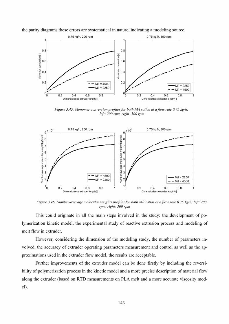
143
the parity diagrams these errors are systematical in nature, indicating a modeling source.
Figure 3.45. Monomer conversion profiles for both M/I ratios at a flow rate 0.75 kg/h;
left: 200 rpm, right: 300 rpm
Figure 3.46. Number-average molecular weights profiles for both M/I ratios at a flow rate 0.75 kg/h; left: 200
rpm, right: 300 rpm
This could originate in all the main steps involved in the study: the development of po-
lymerization kinetic model, the experimental study of reactive extrusion process and modeling of
melt flow in extruder.
However, considering the dimension of the modeling study, the number of parameters in-
volved, the accuracy of extruder operating parameters measurement and control as well as the ap-
proximations used in the extruder flow model, the results are acceptable.
Further improvements of the extruder model can be done firstly by including the reversi-
bility of polymerization process in the kinetic model and a more precise description of material flow
along the extruder (based on RTD measurements on PLA melt and a more accurate viscosity mod-
el).
0 0.2 0.4 0.6 0.8 11
2
3
4
5
6
7
8
9x 10
4
Dimensionless extruder length/[-]
Nu
mb
er-
ave
rag
e m
ole
cula
r w
eig
ht/[k
g/k
mo
l]
0.75 kg/h, 200 rpm
M/I = 4500
M/I = 2250
0 0.2 0.4 0.6 0.8 11
2
3
4
5
6
7
8
9x 10
4
Dimensionless extruder length/[-]
Nu
mb
er-
ave
rag
e m
ole
cula
r w
eig
ht/[k
g/k
mo
l]
0.75 kg/h, 300 rpm
M/I = 2250
M/I = 4500
0 0.2 0.4 0.6 0.8 10
0.2
0.4
0.6
0.8
1
Dimensionless extruder length/[-]
Mon
om
er
co
nve
rsio
n/[-]
0.75 kg/h, 200 rpm
M/I = 4500
M/I = 2250
0 0.2 0.4 0.6 0.8 10
0.2
0.4
0.6
0.8
1
Dimensionless extruder length/[-]
Mon
om
er
co
nve
rsio
n/[-]
0.75 kg/h, 300 rpm
M/I = 2250
M/I = 4500
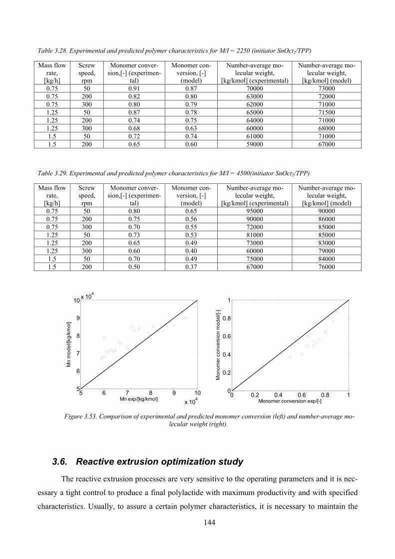
144
Table 3.28. Experimental and predicted polymer characteristics for M/I = 2250 (initiator SnOct2/TPP)
Mass flow rate,
[kg/h]
Screw speed, rpm
Monomer conver-sion,[-] (experimen-
tal)
Monomer con-version, [-]
(model)
Number-average mo-lecular weight,
[kg/kmol] (experimental)
Number-average mo-lecular weight,
[kg/kmol] (model) 0.75 50 0.91 0.87 70000 73000 0.75 200 0.82 0.80 63000 72000 0.75 300 0.80 0.79 62000 71000 1.25 50 0.87 0.78 65000 71500 1.25 200 0.74 0.75 64000 71000 1.25 300 0.68 0.63 60000 68000 1.5 50 0.72 0.74 61000 71000 1.5 200 0.65 0.60 59000 67000
Table 3.29. Experimental and predicted polymer characteristics for M/I = 4500(initiator SnOct2/TPP)
Mass flow rate,
[kg/h]
Screw speed, rpm
Monomer conver-sion,[-] (experimen-
tal)
Monomer con-version, [-]
(model)
Number-average mo-lecular weight,
[kg/kmol] (experimental)
Number-average mo-lecular weight,
[kg/kmol] (model) 0.75 50 0.80 0.65 95000 90000 0.75 200 0.75 0.56 90000 86000 0.75 300 0.70 0.55 72000 85000 1.25 50 0.73 0.53 81000 85000 1.25 200 0.65 0.49 73000 83000 1.25 300 0.60 0.40 60000 79000 1.5 50 0.70 0.49 75000 84000 1.5 200 0.50 0.37 67000 76000
Figure 3.53. Comparison of experimental and predicted monomer conversion (left) and number-average mo-
lecular weight (right)
3.6. Reactive extrusion optimization study
The reactive extrusion processes are very sensitive to the operating parameters and it is nec-
essary a tight control to produce a final polylactide with maximum productivity and with specified
characteristics. Usually, to assure a certain polymer characteristics, it is necessary to maintain the
0 0.2 0.4 0.6 0.8 10
0.2
0.4
0.6
0.8
1
Monomer conversion exp/[-]
Mo
no
me
r co
nve
rsio
n m
od
el/[-
]
5 6 7 8 9 10
x 104
5
6
7
8
9
10x 10
4
Mn exp/[kg/kmol]
Mn
mo
de
l/[kg
/km
ol]
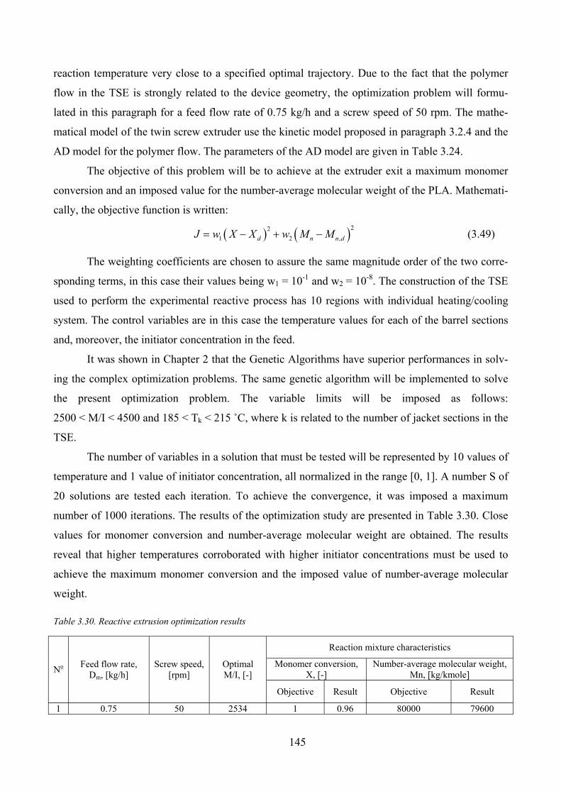
145
reaction temperature very close to a specified optimal trajectory. Due to the fact that the polymer
flow in the TSE is strongly related to the device geometry, the optimization problem will formu-
lated in this paragraph for a feed flow rate of 0.75 kg/h and a screw speed of 50 rpm. The mathe-
matical model of the twin screw extruder use the kinetic model proposed in paragraph 3.2.4 and the
AD model for the polymer flow. The parameters of the AD model are given in Table 3.24.
The objective of this problem will be to achieve at the extruder exit a maximum monomer
conversion and an imposed value for the number-average molecular weight of the PLA. Mathemati-
cally, the objective function is written:
( ) ( )22
1 2 ,d n n dJ w X X w M M= − + − (3.49)
The weighting coefficients are chosen to assure the same magnitude order of the two corre-
sponding terms, in this case their values being w1 = 10-1 and w2 = 10-8. The construction of the TSE
used to perform the experimental reactive process has 10 regions with individual heating/cooling
system. The control variables are in this case the temperature values for each of the barrel sections
and, moreover, the initiator concentration in the feed.
It was shown in Chapter 2 that the Genetic Algorithms have superior performances in solv-
ing the complex optimization problems. The same genetic algorithm will be implemented to solve
the present optimization problem. The variable limits will be imposed as follows:
2500 < M/I < 4500 and 185 < Tk < 215 ˚C, where k is related to the number of jacket sections in the
TSE.
The number of variables in a solution that must be tested will be represented by 10 values of
temperature and 1 value of initiator concentration, all normalized in the range [0, 1]. A number S of
20 solutions are tested each iteration. To achieve the convergence, it was imposed a maximum
number of 1000 iterations. The results of the optimization study are presented in Table 3.30. Close
values for monomer conversion and number-average molecular weight are obtained. The results
reveal that higher temperatures corroborated with higher initiator concentrations must be used to
achieve the maximum monomer conversion and the imposed value of number-average molecular
weight.
Table 3.30. Reactive extrusion optimization results
Reaction mixture characteristics
Monomer conversion, X, [-]
Number-average molecular weight, Mn, [kg/kmole] No
Feed flow rate, Dm, [kg/h]
Screw speed, [rpm]
Optimal M/I, [-]
Objective Result Objective Result
1 0.75 50 2534 1 0.96 80000 79600

146
0 0.2 0.4 0.6 0.8 1202
204
206
208
210
212
214
Ba
rre
l te
mp
era
ture
/ [ oC
]
Dimensionless extruder length / [ - ]
Figure 3.47. Optimal temperature profile for the reactive extrusion optimization problem
Figure 3.48 shows a rapid start of the polymerization process in the TSE due to the high
temperatures required on the first two extruder barrel sections. Consequently, the monomer conver-
sion profile has a faster increase in the first half of screw and a slower one on the final zone.
Figure 3.48. Monomer conversion and number-average molecular weights
profiles calculated with the optimal policy
3.7. Conclusions
The objectives of this chapter were to realize a comprehensive modeling study for L-lactide
reactive extrusion polymerization process based on experimental investigations. The first step of the
study was to develop a kinetic model of L-lactide polymerization, necessary to build the mathe-
matical model of the reactive extrusion polymerization process. The primary approach in develop-
ing the kinetic model has involved the L-lactide polymerization process initiated by only stannous
octoate. Experimental studies using commercial purity of monomer and initiator were carried out at
0 0.2 0.4 0.6 0.8 10
0.2
0.4
0.6
0.8
1
Mo
no
me
r co
nve
rsio
n/ [ -
]
Dimensionless extruder length /[ - ]0 0.2 0.4 0.6 0.8 1
2
3
4
5
6
7
8
9x 10
4
Nu
mb
er-
ave
rag
e m
ole
cu
lar
we
igh
t / [ kg
/km
ole
Dimensionless extruder length / [ - ]
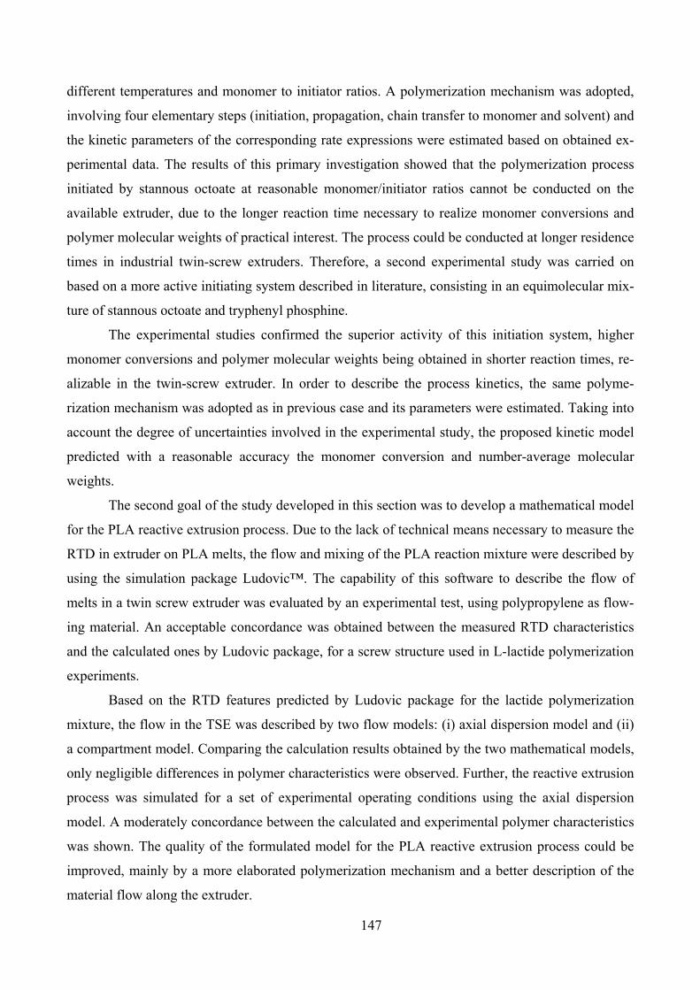
147
different temperatures and monomer to initiator ratios. A polymerization mechanism was adopted,
involving four elementary steps (initiation, propagation, chain transfer to monomer and solvent) and
the kinetic parameters of the corresponding rate expressions were estimated based on obtained ex-
perimental data. The results of this primary investigation showed that the polymerization process
initiated by stannous octoate at reasonable monomer/initiator ratios cannot be conducted on the
available extruder, due to the longer reaction time necessary to realize monomer conversions and
polymer molecular weights of practical interest. The process could be conducted at longer residence
times in industrial twin-screw extruders. Therefore, a second experimental study was carried on
based on a more active initiating system described in literature, consisting in an equimolecular mix-
ture of stannous octoate and tryphenyl phosphine.
The experimental studies confirmed the superior activity of this initiation system, higher
monomer conversions and polymer molecular weights being obtained in shorter reaction times, re-
alizable in the twin-screw extruder. In order to describe the process kinetics, the same polyme-
rization mechanism was adopted as in previous case and its parameters were estimated. Taking into
account the degree of uncertainties involved in the experimental study, the proposed kinetic model
predicted with a reasonable accuracy the monomer conversion and number-average molecular
weights.
The second goal of the study developed in this section was to develop a mathematical model
for the PLA reactive extrusion process. Due to the lack of technical means necessary to measure the
RTD in extruder on PLA melts, the flow and mixing of the PLA reaction mixture were described by
using the simulation package Ludovic™. The capability of this software to describe the flow of
melts in a twin screw extruder was evaluated by an experimental test, using polypropylene as flow-
ing material. An acceptable concordance was obtained between the measured RTD characteristics
and the calculated ones by Ludovic package, for a screw structure used in L-lactide polymerization
experiments.
Based on the RTD features predicted by Ludovic package for the lactide polymerization
mixture, the flow in the TSE was described by two flow models: (i) axial dispersion model and (ii)
a compartment model. Comparing the calculation results obtained by the two mathematical models,
only negligible differences in polymer characteristics were observed. Further, the reactive extrusion
process was simulated for a set of experimental operating conditions using the axial dispersion
model. A moderately concordance between the calculated and experimental polymer characteristics
was shown. The quality of the formulated model for the PLA reactive extrusion process could be
improved, mainly by a more elaborated polymerization mechanism and a better description of the
material flow along the extruder.

148
An optimization problem for a set of operating conditions was formulated and solved using
a genetic algorithm. As expected, the results revealed that relatively high temperatures and initiator
concentrations are required to achieve high monomer conversions.

149
4. General Conclusions

150
This work presented a theoretical and experimental study treating the subjects of modeling
and optimization of tubular polymerization reactors. The research studies had the following main
objectives:
Ü Comparison of the performances or two widely used numerical algorithms in the optimization
of polymerization tubular reactors, Pontryagin’s Minimum Principle (MP) and a Genetic Algo-
rithm (GA), based on polymerization process with a well known kinetics.
Ü Development of a mathematical modeling study and an optimization application for the L-
lactide polymerization process in a co-rotating twin screw extruder.
Original results
The theoretical studies associated to the first objective consisted of the following main steps
and led to the following conclusions:
Ü As case study for the comparison of MP and GA, it was selected the MMA solution polym-
erization process, a chemical system well described in literature. The main published kinetic
models for this process were reviewed and compared in terms of monomer conversion and
number-average molecular weights, by plug-flow reactor simulation in identical operating
conditions. Among the published kinetic models tested, the results showed as the most repre-
sentative, the kinetic model published by Baillagou et Soong (1985).
Ü Based on the kinetic model published by Baillagou et Soong (1985), mathematical models
and numerical simulation procedures for the MMA tubular polymerization reactor were de-
veloped considering plug-flow and laminar flow regimes. The simulation results are high-
lighting significant limitations of the laminar flow reactor, due to the strong decrease of fluid
velocity near the reactor wall. As consequence, the reaction times in the center of the reactor
tube are much lower than at the periphery and the contribution of the central zone to the
chemical transformation becomes less important, resulting in a non-uniform utilization of the
reaction volume. Due to lower velocities and higher reaction times near the wall, higher mo-
nomer conversions and polymer concentrations emerge in this region than in the core of tube.
These limitations are growing with the monomer concentration in the feed, becoming hardly
acceptable, particularly at high monomer to solvent ratios.
Ü It was formulated an optimization problem for the tubular MMA polymerization reactor,
based on plug-flow hypothesis, having as objective to identify the reaction temperature pro-
file corresponding to a polymer product with given properties at a given monomer conver-
sion. This is an average difficulty optimization problem for a polymerization tubular reactor.
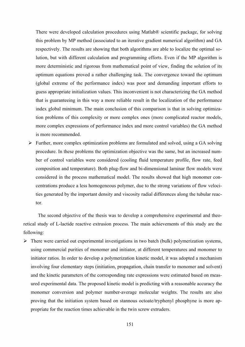
151
There were developed calculation procedures using Matlab® scientific package, for solving
this problem by MP method (associated to an iterative gradient numerical algorithm) and GA
respectively. The results are showing that both algorithms are able to localize the optimal so-
lution, but with different calculation and programming efforts. Even if the MP algorithm is
more deterministic and rigorous from mathematical point of view, finding the solution of its
optimum equations proved a rather challenging task. The convergence toward the optimum
(global extreme of the performance index) was poor and demanding important efforts to
guess appropriate initialization values. This inconvenient is not characterizing the GA method
that is guaranteeing in this way a more reliable result in the localization of the performance
index global minimum. The main conclusion of this comparison is that in solving optimiza-
tion problems of this complexity or more complex ones (more complicated reactor models,
more complex expressions of performance index and more control variables) the GA method
is more recommended.
Ü Further, more complex optimization problems are formulated and solved, using a GA solving
procedure. In these problems the optimization objective was the same, but an increased num-
ber of control variables were considered (cooling fluid temperature profile, flow rate, feed
composition and temperature). Both plug-flow and bi-dimensional laminar flow models were
considered in the process mathematical model. The results showed that high monomer con-
centrations produce a less homogeneous polymer, due to the strong variations of flow veloci-
ties generated by the important density and viscosity radial differences along the tubular reac-
tor.
The second objective of the thesis was to develop a comprehensive experimental and theo-
retical study of L-lactide reactive extrusion process. The main achievements of this study are the
following:
Ü There were carried out experimental investigations in two batch (bulk) polymerization systems,
using commercial purities of monomer and initiator, at different temperatures and monomer to
initiator ratios. In order to develop a polymerization kinetic model, it was adopted a mechanism
involving four elementary steps (initiation, propagation, chain transfer to monomer and solvent)
and the kinetic parameters of the corresponding rate expressions were estimated based on meas-
ured experimental data. The proposed kinetic model is predicting with a reasonable accuracy the
monomer conversion and polymer number-average molecular weights. The results are also
proving that the initiation system based on stannous octoate/tryphenyl phosphyne is more ap-
propriate for the reaction times achievable in the twin screw extruders.

152
Ü The flow of the L-lactide/polylactide mixture was investigated by experimental and modeling
studies. Due to the lack of technical means necessary to measure the RTD in extruder on PLA
melts, the flow and mixing of the PLA reaction mixture were described by using the simulation
package Ludovic™. The capability of this software to predict the flow of polymer melts in a
twin screw extruder is proved by an experimental test, using polypropylene as flowing material.
An acceptable concordance was obtained between the measured RTD characteristics and the
calculated ones by Ludovic package, for a screw structure used in L-lactide polymerization ex-
periments.
Ü Based on the RTD features predicted by Ludovic package for the lactide polymerization mix-
ture, the flow of L-lactide/PLA melt in the TSE is described by two flow models: (i) the axial
dispersion model and (ii) a compartment type model. Comparing the calculation results based
on the two flow models, only negligible differences in polymer characteristics were observed.
Further, the reactive extrusion process was simulated for a set of experimental operating condi-
tions using the axial dispersion model. A moderately good concordance between the calculated
and experimental polymer characteristics is revealed. The quality of the formulated model for
the PLA reactive extrusion process could be improved, mainly by a more elaborated polymeri-
zation mechanism and a better description of the material flow along the extruder.
Ü An optimization problem was further developed and solved, concerning the optimization of the
thermal regime for the L-lactide reactive extrusion process. The results showed that rather high
temperatures and initiator concentrations are required, in order to achieve total monomer con-
version.
Suggestions for future work
The present study has inherent limitations generated by the conditions and working domains
of experimental investigations, their accuracy and the simplification hypotheses introduced in the
theoretical developments. Consequently, future developments could improve the quality of results,
particularly regarding the modeling of the L-lactide polymerization process by reactive extrusion.
A first direction for further development is regarding the experimental and theoretical study
of the process kinetics. Also, a more accurate investigation could be performed, in conditions of
higher purity of materials and larger domains of working conditions. The quality of the kinetic
model could be improved by taking into account the de-polymerization reactions, as well as inter
and intra-molecular transesterification reactions. A design of experiments procedure can be imple-
mented to discriminate among the degree of influence of different process parameters on the po-
lymerization.

153
The second direction of possible improvements concerns the flow modeling of the reactive
extrusion process. An experimental study of RTD of polylactide synthesis mixture in the extruder
using an appropriate tracer could provide further information concerning the melt material flow and
mixing in the TSE. The flow and mixing modeling can also be improved by a more complete rheo-
logical study of L-lactide/polylactide mixture, giving a better description of viscosity dependence
on the temperature and composition.
Finally an optimization dynamic study for the start-up and shut-down steps, the study of the
parameter sensitivity and of the reactor operating stationary points can provide extensive data for
the considered polymerization process.

154

155
5. Appendix 1: PLA reactive extrusion simulation by Ludovic.
RTD curves and compartment model data
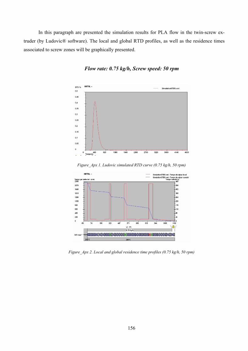
156
In this paragraph are presented the simulation results for PLA flow in the twin-screw ex-
truder (by Ludovic® software). The local and global RTD profiles, as well as the residence times
associated to screw zones will be graphically presented.
Flow rate: 0.75 kg/h, Screw speed: 50 rpm
Figure_Apx 1. Ludovic simulated RTD curve (0.75 kg/h, 50 rpm)
Figure_Apx 2. Local and global residence time profiles (0.75 kg/h, 50 rpm)
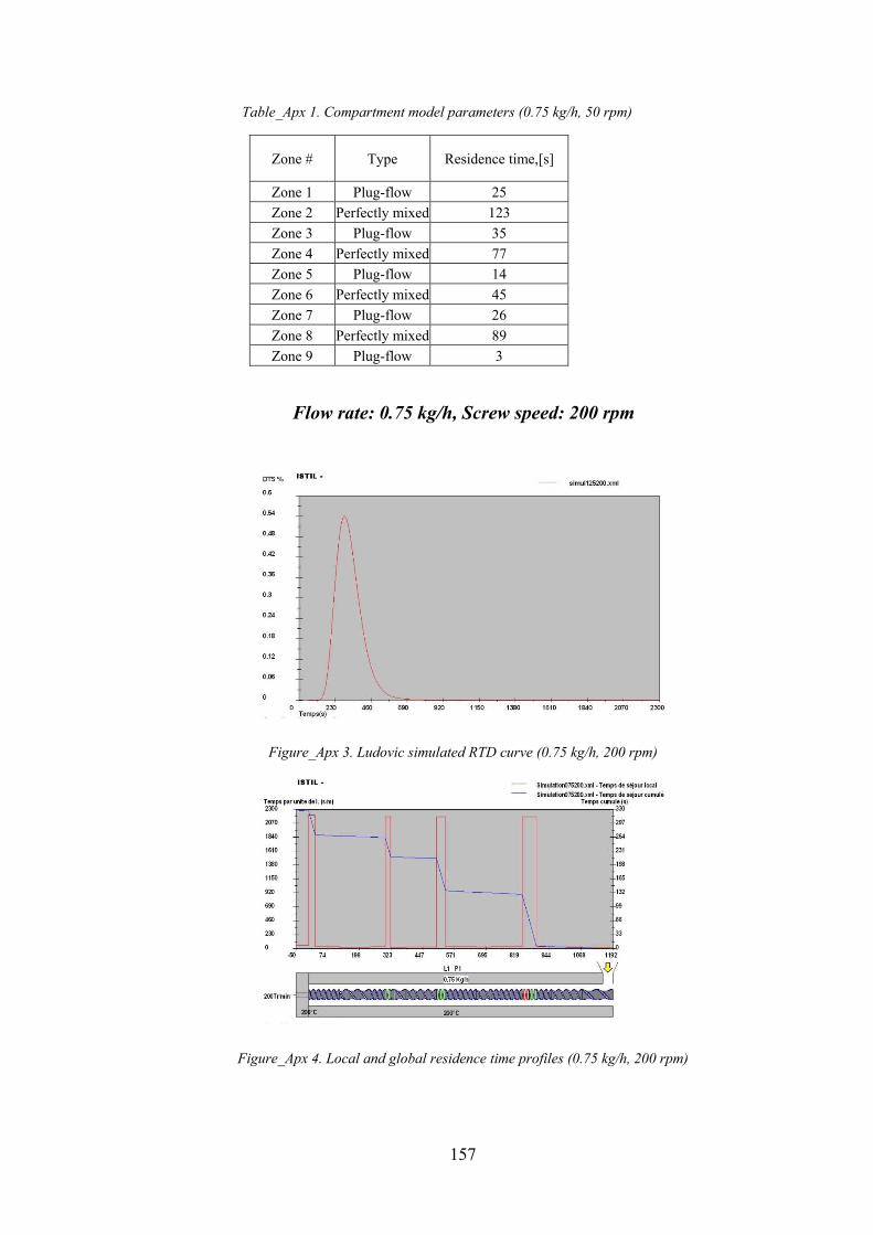
157
Table_Apx 1. Compartment model parameters (0.75 kg/h, 50 rpm)
Zone # Type Residence time,[s]
Zone 1 Plug-flow 25
Zone 2 Perfectly mixed 123
Zone 3 Plug-flow 35
Zone 4 Perfectly mixed 77
Zone 5 Plug-flow 14
Zone 6 Perfectly mixed 45
Zone 7 Plug-flow 26
Zone 8 Perfectly mixed 89
Zone 9 Plug-flow 3
Flow rate: 0.75 kg/h, Screw speed: 200 rpm
Figure_Apx 3. Ludovic simulated RTD curve (0.75 kg/h, 200 rpm)
Figure_Apx 4. Local and global residence time profiles (0.75 kg/h, 200 rpm)
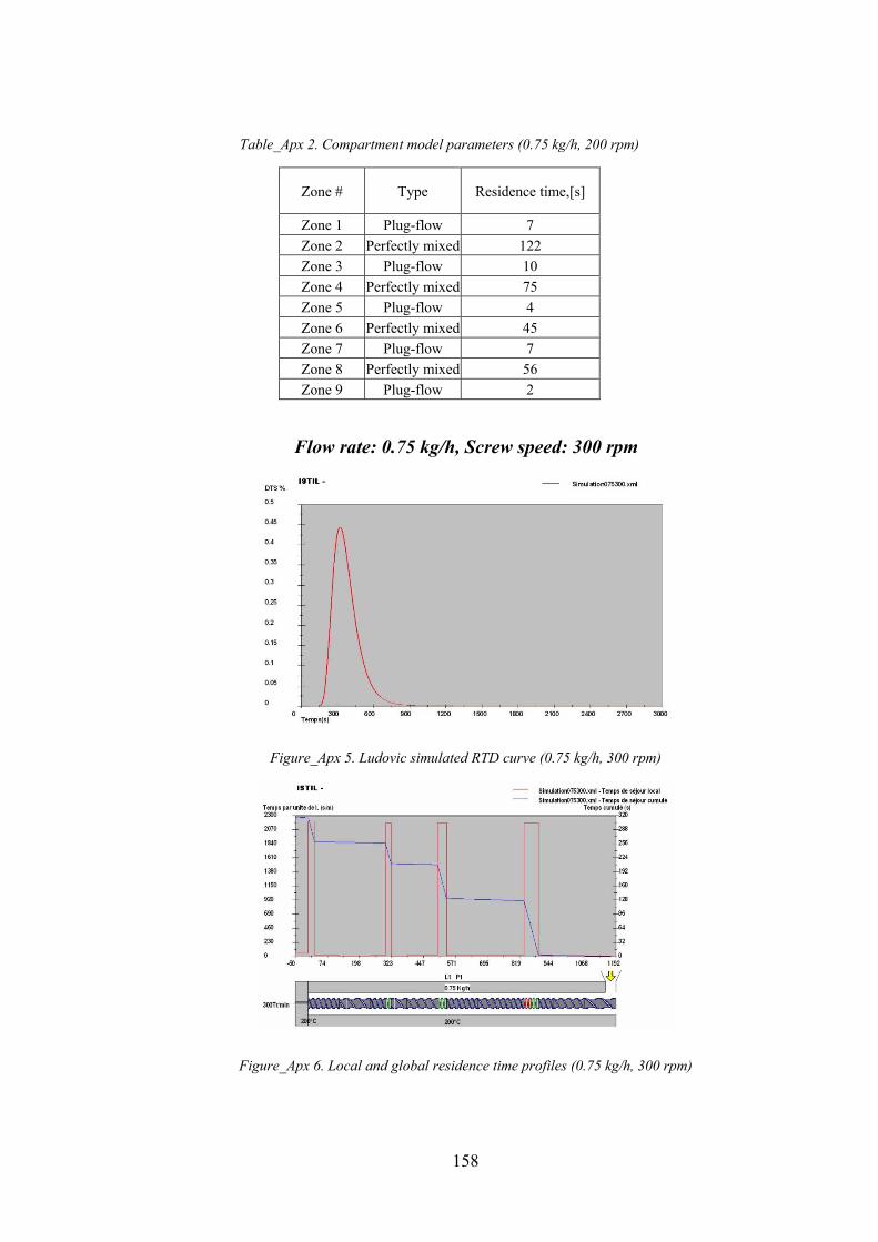
158
Table_Apx 2. Compartment model parameters (0.75 kg/h, 200 rpm)
Zone # Type Residence time,[s]
Zone 1 Plug-flow 7
Zone 2 Perfectly mixed 122
Zone 3 Plug-flow 10
Zone 4 Perfectly mixed 75
Zone 5 Plug-flow 4
Zone 6 Perfectly mixed 45
Zone 7 Plug-flow 7
Zone 8 Perfectly mixed 56
Zone 9 Plug-flow 2
Flow rate: 0.75 kg/h, Screw speed: 300 rpm
Figure_Apx 5. Ludovic simulated RTD curve (0.75 kg/h, 300 rpm)
Figure_Apx 6. Local and global residence time profiles (0.75 kg/h, 300 rpm)
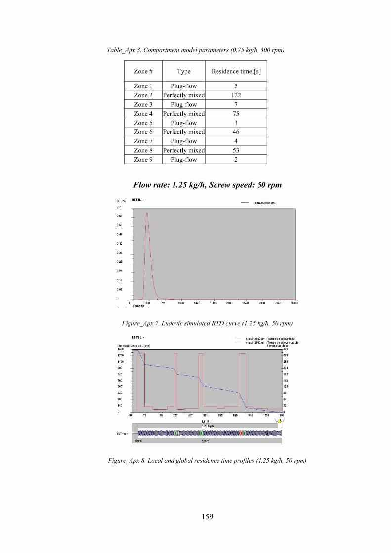
159
Table_Apx 3. Compartment model parameters (0.75 kg/h, 300 rpm)
Zone # Type Residence time,[s]
Zone 1 Plug-flow 5
Zone 2 Perfectly mixed 122
Zone 3 Plug-flow 7
Zone 4 Perfectly mixed 75
Zone 5 Plug-flow 3
Zone 6 Perfectly mixed 46
Zone 7 Plug-flow 4
Zone 8 Perfectly mixed 53
Zone 9 Plug-flow 2
Flow rate: 1.25 kg/h, Screw speed: 50 rpm
Figure_Apx 7. Ludovic simulated RTD curve (1.25 kg/h, 50 rpm)
Figure_Apx 8. Local and global residence time profiles (1.25 kg/h, 50 rpm)
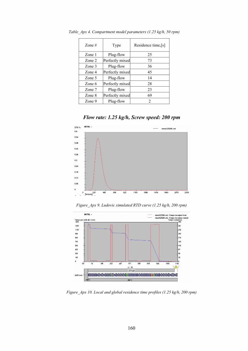
160
Table_Apx 4. Compartment model parameters (1.25 kg/h, 50 rpm)
Zone # Type Residence time,[s]
Zone 1 Plug-flow 25
Zone 2 Perfectly mixed 73
Zone 3 Plug-flow 36
Zone 4 Perfectly mixed 45
Zone 5 Plug-flow 14
Zone 6 Perfectly mixed 28
Zone 7 Plug-flow 23
Zone 8 Perfectly mixed 69
Zone 9 Plug-flow 2
Flow rate: 1.25 kg/h, Screw speed: 200 rpm
Figure_Apx 9. Ludovic simulated RTD curve (1.25 kg/h, 200 rpm)
Figure_Apx 10. Local and global residence time profiles (1.25 kg/h, 200 rpm)
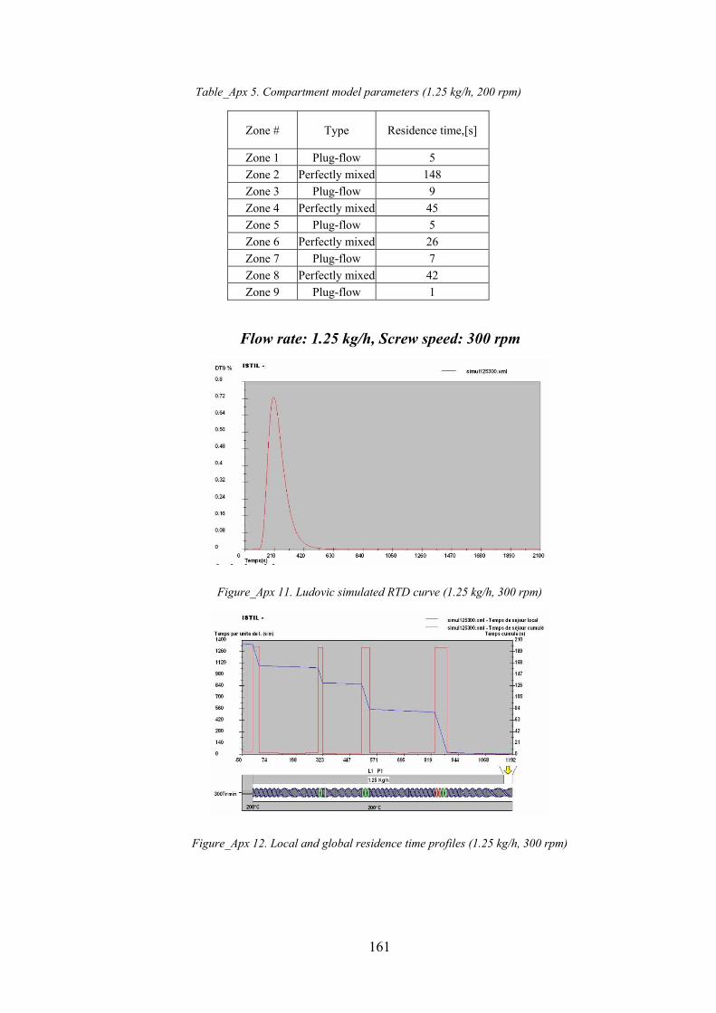
161
Table_Apx 5. Compartment model parameters (1.25 kg/h, 200 rpm)
Zone # Type Residence time,[s]
Zone 1 Plug-flow 5
Zone 2 Perfectly mixed 148
Zone 3 Plug-flow 9
Zone 4 Perfectly mixed 45
Zone 5 Plug-flow 5
Zone 6 Perfectly mixed 26
Zone 7 Plug-flow 7
Zone 8 Perfectly mixed 42
Zone 9 Plug-flow 1
Flow rate: 1.25 kg/h, Screw speed: 300 rpm
Figure_Apx 11. Ludovic simulated RTD curve (1.25 kg/h, 300 rpm)
Figure_Apx 12. Local and global residence time profiles (1.25 kg/h, 300 rpm)
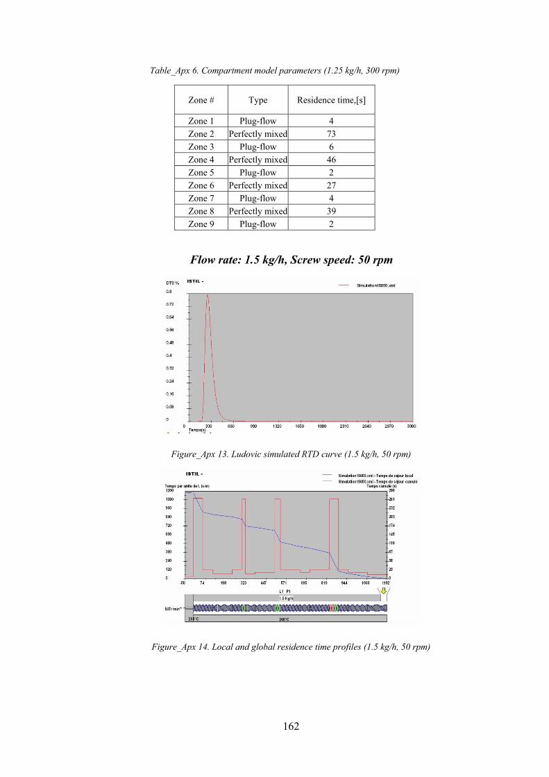
162
Table_Apx 6. Compartment model parameters (1.25 kg/h, 300 rpm)
Zone # Type Residence time,[s]
Zone 1 Plug-flow 4
Zone 2 Perfectly mixed 73
Zone 3 Plug-flow 6
Zone 4 Perfectly mixed 46
Zone 5 Plug-flow 2
Zone 6 Perfectly mixed 27
Zone 7 Plug-flow 4
Zone 8 Perfectly mixed 39
Zone 9 Plug-flow 2
Flow rate: 1.5 kg/h, Screw speed: 50 rpm
Figure_Apx 13. Ludovic simulated RTD curve (1.5 kg/h, 50 rpm)
Figure_Apx 14. Local and global residence time profiles (1.5 kg/h, 50 rpm)
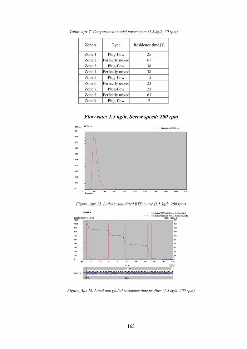
163
Table_Apx 7. Compartment model parameters (1.5 kg/h, 50 rpm)
Zone # Type Residence time,[s]
Zone 1 Plug-flow 25
Zone 2 Perfectly mixed 61
Zone 3 Plug-flow 36
Zone 4 Perfectly mixed 38
Zone 5 Plug-flow 15
Zone 6 Perfectly mixed 23
Zone 7 Plug-flow 23
Zone 8 Perfectly mixed 63
Zone 9 Plug-flow 2
Flow rate: 1.5 kg/h, Screw speed: 200 rpm
Figure_Apx 15. Ludovic simulated RTD curve (1.5 kg/h, 200 rpm)
Figure_Apx 16. Local and global residence time profiles (1.5 kg/h, 200 rpm)

164
Table_Apx 8. Compartment model parameters (1.5 kg/h, 200 rpm)
Zone # Type Residence time,[s]
Zone 1 Plug-flow 6
Zone 2 Perfectly mixed 61
Zone 3 Plug-flow 9
Zone 4 Perfectly mixed 37
Zone 5 Plug-flow 4
Zone 6 Perfectly mixed 23
Zone 7 Plug-flow 7
Zone 8 Perfectly mixed 37
Zone 9 Plug-flow 1
165
6. List of publications
A. Journal papers
• J. P. Puaux, I. Banu, I. Nagy, G. Bozga, A study of L-lactide ring-opening polymerization
kinetics, Macromolecular Symposia, 259 (1), 2007, 318 – 326.
• Banu I., G. Bozga, I. Nagy, J. P. Puaux, A Comparison of Variational and Genetic Algorithm
Performances in the Optimization of a Polymerization Process, Chemical Engineering and
Technology, 31(10), 2008, 1516-1525.
• Banu I., S. Bildea, G. Bozga, J. P. Puaux, Simulation of a laminar flow tubular reactor, Studia
Universitatis Babes-Bolyai Chemia, 1, 2009, 227-242.
• Banu I., N. D. Stanciu, J. P. Puaux, G. Bozga, A study of L-lactide ring-opening polymerization
in molten state, U.P.B. Sci. Bull., Series B, 71(2), 2009.
• Banu I., J. P. Puaux, G. Bozga, I. Nagy, Modeling of L-lactide polymerization by reactive ex-
trusion, Macromolecular Symposia, 2009, accepted for publication.
B. Papers published in the proceedings of national and international conferences
• Banu I., G. Bozga, J. P. Puaux, Optimization of a molecular weight distribution in a batch free
radical polymerization process, Proceedings of Romanian International Conference of Chemis-
try and Chemical Engineering (RICCCE 14), 22 – 24 September 2005, vol. 3, 174 – 181.
• Banu I., G. Bozga, I. Nagy, J. P. Puaux, A comparison of the Minimum Principle and Genetic
Algorithms in the optimization of the thermal regime for methyl methacrylate polymerization in
solution, 18th International Congress of Chemical and Process Engineering, 24-28 august 2008,
Prague, Czech Republic (published on CD).
C. National and international conferences communications
• Banu I., G. Bozga, Optimization of a batch polymerization reactor, CAPE Forum, 25-26 Feb-
ruary 2005, Cluj-Napoca, Romania.
• J. P. Puaux, I. Banu, I. Nagy, G. Bozga, Optimization of a tubular reactor for MMA polymeri-
zation in solution, Vingtiemes Entretiens du Centre Jacques Cartier, 3 – 4 December 2007,
Lyon, France
• Banu I., G. Bozga, I. Nagy, J. P. Puaux, Optimization of a tubular polymerization reactor,
Polymer Reaction Engineering 7, May 3-9, 2009, Niagara Falls, Ontario, Canada.
• Banu I., J. P. Puaux, G. Bozga, I. Nagy, Modeling of L-lactide polymerization by reactive ex-
166
trusion, Polymer Reaction Engineering 7, May 3-9, 2009, Niagara Falls, Ontario, Canada.
7. References
1. Vega, M.P., E.L. Lima, and J.C. Pinto, Control of a loop polymerization reactor using neu-
ral networks. Brazilian Journal of Chemical Engineering, 2000. 17: p. 471-482. 2. Embirucu, M., E.L. Lima, and J.C. Pinto, A survey of advanced control of polymerization
reactors. Polymer Engineering and Science, 1996. 36(4): p. 433 - 447. 3. Asua, J.M., ed. Polymer reaction engineering. 2007, Blackwell Publishing Ltd.: Oxford. 4. Ullmann's Encyclopedia of Industrial Chemistry. 1997. 5. Kirk-Othmer Encyclopedia of Chemical Technology. 2008, John Wiley & Sons. 6. Odian, G., Principles of Polymerization. 2004, John Wiley & Sons, Inc.: New Jersey. 7. Schork, F.J., P.B. Deshpande, and K.W. Leffew, Control of polymerization reactors. 1993,
New York: M. Dekker. 8. Bozga, G. and I. Nagy, Reacteurs Chimiques. Theorie et applications. 2001, Bucuresti: Ed.
Bren. 9. Kricheldorf, H.R., O. Nuyken, and G. Swift, eds. Handbook of Polymer Synthesis. 2nd ed.
2005, Marcel Dekker: New York. 10. Bauer, W., Processes for producing acrylic acid esters, R.a.H.A.-. Gesellschaft, Editor.
1928: United States. p. 1. 11. Maschio, G., T. Bello, and C. Scali, Optimal operation strategies to control the molecular
weight distribution of polymer products. Chemical Engineering Science, 1994. 49(24B): p. 5071-5086.
12. Schmidt, A.D. and W.H. Ray, The dynamic behavior of continuous polymerization reactors
- I. Isothermal solution polymerization in a CSTR. Chemical Engineering Science, 1981. 36: p. 1401 - 1410.
13. Chiu, W.Y., G.M. Carrat, and D.S. Soong, A computer model for the gel effect in free-
radical polymerization. Macromolecules, 1983. 16: p. 348-357. 14. Carter, J., Modeling the polymerization of methylmethacrylate in wood under nonisothermal
conditions, in Graduate Academic Unit of Chemical Engineering. 2000, University of New Brunswick.
15. Tulig, T. and M. Tirrell, Toward a Molecular Theory of the Trommsdorff Effect. Macro-molecules, 1981. 14(5): p. 1501-1511.
16. Baillagou, P.E. and D.S. Soong, Majors factors contributing to the nonlinear kinetics on
free-radical polymerization. Chemical Engineering Science, 1985. 40(1): p. 75 - 86. 17. Baillagou, P.E. and D.S. Soong, Molecular weight distribution of products of free radical
nonisothermal polymerization with gel effect. Simulation for polymerization of poly(methyl
methacrylate). Chemical Engineering Science 1985. 40(1): p. 87-104. 18. Nising, P., High temperature radical polymerization of methylmethacrylate in a continous
pilot scale process. 2006, Ecole Polythechnique Federale de Lausanne: Lausanne. 19. F. Fenouillot, J.T., T. Rimlinger,, Polymerization of methyl methacrylate at high tempera-
ture with 1-butanethiol as chain transfer agent. Journal of Applied Polymer Science, 1999. 72(12): p. 1589-1599.
20. Ahn, S.-M., S.-P. Chang, and H.-K. Rhee, Application of optimal temperature trajectory to
batch PMMA polymerization reactor. Journal of Applied Polymer Science 1998. 69: p. 59 - 68.
21. Chang, J.-S. and J.-L. Lai, Computation of optimal temperature policy for molecular weight
control in a batch polymerization reactor. Ind. Eng. Chem. Res., 1992. 31: p. 861 - 868. 22. Chang, J.-S. and P.-S. Liao, Molecular weight control of a batch polymerization reactor:
experimental study. Ind. Eng. Chem. Res., 1999. 38: p. 144 - 153.
167
23. Ponnuswamy, S.R., S.L. Shah, and C.A. Kiparissides, Computer optimal control of batch
polymerization reactors. Ind. Eng. Chem. Res., 1987. 26(11): p. 2229 - 2236. 24. Crowley, T. and K.Y. Choi, Calculation of molecular weight distribution from molecular
weights moments in free radical polymerization. Ind. Eng. Chem. Res, 1997. 36: p. 1419 - 1423.
25. Crowley, T.J. and K.Y. Choi, Discrete optimal control of molecular weight distribution in a
batch free radical polymerization process. Ind. Eng. Chem. Res., 1997. 36: p. 3676-3684. 26. Kiparissides, C., P. Seferlis, G. Mourikas, and A.J. Morris, Online Optimizing Control of
Molecular Weight Properties in Batch Free-Radical Polymerization Reactors. Ind. Eng. Chem. Res., 2002. 41(24): p. 6120-6131.
27. Scali, C., R. Ciari, T. Belo, and G. Maschio, Optimal temperature for the cotrol of the prod-
uct quality in batch polymerization: simulation and experimental results. Journal of Applied Polymer Science, 1995. 55: p. 945 - 959.
28. Mihail, R., Modele cinetice de polireactii. 1986, Bucuresti: Editura Stiintifica si Enciclope-dica.
29. Ponnuswamy, S.R., On-line measurements and control of a batch polymerization reactor. 1984, University of Alberta: Edmonton. p. 252.
30. Husain, A. and A.E. Hamielec, Bulk thermal polymerization of styrene in a tubular reactor -
a computer study. AiChE Symposium Series, 1976. 31. Baillagou, P.E. and D.S. Soong, Free radical polymerization of methyl methacrylate in tu-
bular reactors. Polymer Engineering & Science, 1985. 25(4 ): p. 212 - 231. 32. Lynn, S. and J.E. Huff, Polymerization in a tubular reactor. AIChE Journal, 1971. 17(2): p.
475 - 481. 33. Wyman, C.E. and L.F. Carter, A numerical model for tubular polymerization reactors.
AiChE Symposium Series, 1976. 34. Ghosh, M. and D.W. Foster, A model of a tubular reactor for the continuous polymerization
of styrene: experiements at low molecular weight. AiChE Symposium Series, 1976. 35. Nauman, B.E., ed. Chemical Reactor Design, Optimization, and Scaleup. 2002, McGraw-
Hill 36. Hicks, J., A. Mohan, and W.H. Ray, The optimal control of polymerization reactors. Cana-
dian Journal of Chemical Engineering, 1969. 47: p. 590 - 597. 37. Sacks, M.E., S.I. Lee, and J.A. Biesenberger, Optimal policies for batch, chain addition po-
lymerizations. Chemical Engineering Science, 1972. 27(12). 38. Louie, B.M. and D.S. Soong, Optimization of batch polymerization processes - Narrowing
the MWD. I. Model simulation. Journal of Applied Polymer Science, 1985. 30: p. 3707 - 3749.
39. Takamatsu, T., S. Shioya, and Y. Okada, Molecular weight distribution control in a batch
polymerization reactor. Ind. Eng. Chem. Res., 1988. 27(1): p. 93 - 99. 40. Schmidt, A.D. and A.H. Ray, The dynamic behavior of continuous polymerization reactors-
I. isothermal solution polymerization in a CSTR. Chemical Engineering Science, 1981. 36: p. 1401 - 1410.
41. Kirk, D.E., Optimal Control Theory: An Introduction. Networks Series, ed. R.W. Newcomb. 1970, Englewood Cliffs, New Jersey: Prentice-Hall.
42. Crisan, M.V. and S.P. Agachi, Elemente de teoria sistemelor. 2002, Cluj-Napoca: E. RISO-PRINT.
43. Lucaci, A.I. and P.S. Agachi, Optimizarea proceselor din industria chimica. 2002, Bucur-esti: Ed. Tehnica.
44. Bryson, A.E. and Y.-C. Ho, Applied Optimal Control. 1969, Waltham, Massachusetts: Blaisdell Publishing Company.
45. Chakravarti, S., W. Harmon-Ray, and S.X. Zhang, Kinetic study of olefin polymerization
with a supported metallocene catalyst. IV. Comparison of bridged and unbridged catalyst in

168
gas phase. Journal of Applied Polymer Science, 2001. 81(6): p. 1451-1459. 46. Lee, M.H., C. Han, and K.S. Chang, Hierarchical time-optimal control of a continuous co-
polymerization reactor during start-up or grade change operation using genetic algorithms. Computers Chem. Engng., 1997. 21, Suppl.: p. S1037-S1042.
47. Chakravarthy, S.S.S., D.N. Saraf, and S.K. Gupta, Use of genetic algorithms in the optimi-
zation of free radical polymerizations exhibiting the trommsdorff effect. Journal of Applied Polymer Science, 1997. 63(4): p. 529-548.
48. Haupt, R.L. and S.E. Haupt, Practical Genetic Algorithms (2nd ed.) Journal of the American Statistical Association. Vol. 100. 2005: American Statistical Association. 1099-1099.
49. Kennedy, J. and W.M. Spears. Matching Algorithms to Problems: An Experimental Test of
the Particle Swarm and Some Genetic Algorithms on the Multimodal Problem Generator. in Evolutionary Computation Proceedings, 1998. IEEE World Congress on Computational In-
telligence., The 1998 IEEE International Conference 4-9 May 1998. 50. Marco, N., et al., A genetic algorithm compared with a gradient-based method for the solu-
tion of an active-control model problem. 1996, Institut National De Recherche En Informa-tique Et En Automatique.
51. Perry, R.H., D.W. Green, and J.O. Maloney, Perry's Chemical Engineer's Handbook. 1997, McGraw Hill: New York.
52. Brandrup, J., E.H. Immergut, and E.A. Grulke, eds. Polymer Handbook. 1999, John Wiley and Sons, Inc. : New York.
53. Banu, I., S. Bildea, G. Bozga, and J.-P. Puaux, Simulation of a laminar flow tubular reactor. Studia Universitatis Babes-Bolyai Chemia, 2009(1): p. 227-242.
54. The MathWorks, I., MATLAB Documentation. 1984-2008. 55. I. Banu, G. Bozga, I. Nagy, and J.-P. Puaux, A Comparison of Variational and Genetic Al-
gorithm Performances in the Optimization of a Polymerization Process. Chemical Engineer-ing and Technology, 2008. 31(10): p. 1516-1525.
56. Logist, F., I.Y. Smets, and J.F. VanImpe, Derivation of generic optimal reference tempera-
ture profiles for steady-state exothermic jacketed tubular reactors. Journal of Process Con-trol, 2008. 18: p. 92-104.
57. Polylactides, in Kirk-Othmer Encyclopedia of Chemical Technology, 5th edition. 2004, John Wiley & Sons, Inc.: New Jersey. p. 297-318.
58. Gruber, P. and M. O'Brien, Polylactides "Natureworks PLA" () Biopolymers, Polyesters III - Applications and Commercial Products, ed. Y. Doi and A. Steinbüchel. Vol. 4. 2002, New York: John Wiley and Sons.
59. Mehta, R., Modeling and Simulation of Poly(Lactic Acid) Polymerization, in Department of
Chemical Engineering. 2007, Deemed University, Thapar Institute of Engineering and Technology: Patiala.
60. Bechthold, I., Technologisch Relevante Aspekte Der Ringöffnungspolymerisation Von L,L-
Dilactid 2003, Fakultät III - Prozesswissenschaften - der Technischen Universität Berlin Berlin.
61. Perepelkin, K.E., Polylactide fibers: fabrication, properties, use, prospects. A review. Fibre Chemistry, 2002. 34(2): p. 85-100.
62. Middleton, C.J. and J.A. Tipton, Synthetic biodegradable polymers as orthopedic devices. Biomaterials, 2000. 21: p. 2335 - 2346.
63. Jacobsen, S., et al., Single-step reactive extrusion of PLLA in a corotating twin-screw ex-
truder promoted by 2-ethylhexanoic acid tin(II) salt and triphenylphosphine. Polymer 2000. 41: p. 3395–3403.
64. Auras, R., B. Harte, and S. Selke, An Overview of Polylactides as Packaging Materials. Macromolecular Bioscience, 2004. 4: p. 835–864.
65. Drumright, R.E., P.R. Gruber, and D.E. Henton, Polylactic Acid Technology. Advanced Ma-terials, 2000. 12(23): p. 1841-1846.

169
66. Kurcok, P., et al., Substituent Effect in Anionic-Polymerization of Beta-Lactones Initiated by
Alkali-Metal Alkoxides. Macromolecular Rapid Communications, 1995. 16(7): p. 513-519. 67. Carlson, T.L. and E.M. Peters-Jr., Low PH lactic acid fermentation. 1997, Cargill, Inc.:
United States. 68. Garlotta, D., A Literature Reviewof Poly (Lactic Acid). Journal of Polymers and the Envi-
ronment, 2001. 9(2): p. 63-84. 69. Seppala, J., J.-F. Selin, and T. Su, Method for producing lactic acid based polyurehtane.
1995, Neste OY: United States. 70. Gruber, P.R., et al., Continuous process for manufacture of a purified lactide. 1993, Cargill,
Incorporated: United States. 71. Gruber, P.R., Poly(lactide) copolymer and process for manufacture thereof. 1994, Cargill,
Incorporated: United States. 72. Gruber, P.R., et al., Continuous process for manufacture of lactide polymers with controlled
optical purity. 1999, Cargill, Incorporated: United States. 73. Gruber, P.R., et al., Continuous process for manufacture of lactide and lactide polymers.
2001, Cargill, Inc.: United States. 74. Gruber, P.R., et al., Continuous process for manufacture of lactide polymers with controlled
optical purity. 2001, Cargill, Inc.: United States. 75. Dechy-Cabaret, O., B. Martin-Vaca, and D. Bourissou, Controlled Ring-Opening Polymeri-
zation of Lactide and Glycolide. Chemical Reviews, 2004. 104(12): p. 6147-6176. 76. Amgoune, A., C.M. Thomas, T. Roisnel, and J.F. Carpentier, Ring-opening polymerization
of lactide with group 3 metal complexes supported by dianionic alkoxy-amino-bisphenolate
ligands: Combining high activity, productivity, and selectivity. Chemistry - A European Journal, 2006. 12(1): p. 169-179.
77. Chamberlain, B.M., et al., Polymerization of lactide with zinc and magnesium beta-
diiminate complexes: Stereocontrol and mechanism. Journal of the American Chemical So-ciety, 2001. 123(14): p. 3229-3238.
78. Wu, J.C., et al., Ring-opening polymerization of lactide initiated by magnesium and zinc
alkoxides. Polymer, 2005. 46(23): p. 9784-9792. 79. Stolt, M. and A. Sodergard, Use of Monocarboxylic Iron Derivatives in the Ring-Opening
Polymerization of L-Lactide. Macromolecules, 1999. 32: p. 6412-6417. 80. O'Keefe, B.J., S.M. Monnier, M.A. Hillmyer, and W.B. Tolman, Rapid and controlled po-
lymerization of lactide by structurally characterized ferric alkoxides. Journal of the Ameri-can Chemical Society, 2001. 123(2): p. 339-340.
81. Chrisholm, M.H., J.C. Gallucci, and C. Krempner, Ring-opening polymerization of L-lactide
by organotin(IV)alkoxides, R2Sn(OPri)2: Estimation of the activation parameters. Polyhe-
dron 2007. 26: p. 4436-4444. 82. Storey, R.F., et al., Soluble Tin(II) Macroinitiator Adducts for the Controlled Ring-Opening
Polymerization of Lactones and Cyclic Carbonates. Journal of Polymer Science. Part A: Polymer Chemistry, 2002. 40: p. 3434-3442.
83. Mehta, R., V. Kumar, H. Bhunia, and S.N. Upadhyay, Synthesis of Poly (Lactic Acid): A
Review. Journal of Macromolecular Science Part C: Polymer Reviews, 2005. 45: p. 325-349. 84. Mehta, R., V. Kumar, and S.N. Upadhyay, Mathematical Modeling of the Poly(lactic
acid)Ring-Opening Polymerization Kinetics. Polymer-Plastics Technology and Engineering, 2007. 46(3): p. 257 — 264.
85. Wang, C., H. Li, and X. Zhao, Ring opening polymerization of L – lactide initiated by
creatinine. Biomaterials, 2004. 25: p. 5797 – 5801. 86. Stridsberg, K.M., M. Ryner, and A.-C. Albertsson, Controlled Ring-Opening Polymeriza-
tion: Polymers with designed Macromolecular Architecture, in Degradable Aliphatic Poly-
esters. 2001. p. 41-65. 87. Wu, J., T.-L. Yu, C.-T. Chen, and C.-C. Lin, Recent developments in main group metal

170
complexes catalyzed/initiated polymerization of lactides and related cyclic esters. Coordina-tion Chemistry Reviews, 2006. 250(5-6): p. 602-626.
88. Kricheldorf, H.R., M. Berl, and N. Scharnagl, Poly(lactones). 9. Polymerization Mechanism
of Metal Alkoxide Initiated Polymerizations of Lactide and Various Lactones Macromole-cules, 1988. 21: p. 286-293
89. Degee, P., P. Dubois, and R. Jerome, Bulk polymerization of lactides initiated by aluminium
isopropoxide. Macromol. Chem. Phys. , 1997. 198: p. 1985-1995. 90. Degee, P., P. Dubois, and R. Jerome, Bulk polymerization of lactides initiated by aluminium
isopropoxide, 3 a)
Thermal stability and viscoelastic properties Macromol. Chem. Phys., 1997. 198: p. 1985-1995.
91. Degee, P., P. Dubois, and R. Jerome, Bulk polymerization of lactides initiated by aluminium
isopropoxide, 2 a)
Beneficial effect of Lewis bases and transfer agents Macromol. Chem. Phys., 1997. 198: p. 1973-1984.
92. Degee, P., et al., Beneficial effect of trypheniphosphine on the bulk polymerization of L, L –
lactide promoted by 2 – ethyl hexanoic acid tin(II)salt. Journal of Polymer Science, Part A: Polymer Chemistry, 1999. 37: p. 2413 – 2420.
93. Jacobsen, S., et al., Single-step reactive extrusion of PLLA in a corotating twin-screw ex-
truder promoted by 2-ethylhexanoic acid tin(II) salt and triphenylphosphine. Polymer, 2000. 41(9): p. 3395-3403.
94. Kricheldorf, H.R., Tin-initiated polymerizations of lactones: mechanistic and preparative
aspects. Macromol. Symp., 2000. 153: p. 55-65. 95. Eenink, M.J.D., Synthesis of biodegradable polymers and development of biodegradable
hollow fibres for the controlled release of drugs. 1987, Twente University. 96. Lian-xi, C., W. Jun, F. Jie, and L. Jia-heng, The syntheses and properties of poly( L -
lactide). Wuhan University Journal of Natural Sciences, 2002. 7(4): p. 473-476. 97. Nijenhuis, A.J., D.W. Grijpma, and A.J. Pennings, Lewis acid catalyzed polymerization of
L-lactide. Kinetic and mechanism of the bulk polymerization. Macromolecules, 1992. 25: p. 6419 – 6424.
98. Khanna, A., Y. Sudha, S. Pillai, and S. Rath, Molecular modeling studies of poly lactic acid
initiation mechanisms. Journal of Molecular Modeling, 2008. 14(5): p. 367-374. 99. Moller, M., et al., Stannous (II) trifluoromethane sulphonate: A versatile catalyst for the
controlled ring-opening polymerization of lactides: formation of stereoregular surfaces
from polylactides “brushes”. Journal of Polymer Science: Part A: Polymer Chemistry, 2001. 39: p. 3529 – 3538.
100. Schwach, G., J. Coudane, R.Engel, and M.Vert, Ring Opening Polymerization of D,L-
Lactide in the Presence of Zinc Metal and Zinc Lactate. Polymer International, 1998. 46: p. 177-182.
101. Schwach, G., J. Coudane, R. Engel, and M. Vert, More about the polymerization of lactides
in the presence of stannous octoate. Journal of Polymer Science. Part A: Polymer Chemis-try, 1997. 35: p. 3431 – 3440.
102. Kricheldorf, H.R. and I. Kreiser-Saunders, Polylactones, 19 a)
Anionic polymerization of L-
lactide in solution. Makromol. Chem., 1990. 191: p. 1057-1066 103. Zhang, H., U.P. Wyss, D. Pichora, and M. Goosen, An investigation of the synthesis and
thermal stability of poly(D,L-lactide). Polymer Bulletin, 1992: p. 623 - 629. 104. Zhang, X., D.A. Macdonald, M. Goosen, and K. McAuley, Mechanism of lactide polymeri-
zation in the presence of stannous octoate: The efect of hydroxy and carboxylic acid sub-
stances. Journal of Polymer Science: Part A: Polymer Chemistry, 1994. 32: p. 2965 - 2970. 105. Kricheldorf, H.R., I. Kreiser – Saunders, and A. Stricker, Polylactones 48. SnOct2 - initiated
polymerizations of lactide: A mechanistic study. Macromolecules, 2000. 23: p. 702 – 709. 106. Kowalski, A., A. Duda, and S. Penczek, Kinetics and mechanism of cyclic esters polymeri-
zation initiated with tin(II) octoate: 3. Polymerization of L, L – Dilactide. Macromolecules,
171
2000. 33: p. 7359 – 7270. 107. Kowalski, A., A. Duda, and S. Penczek, Kinetics and mechanism of cyclic esters polymeri-
zation initiated with tin(II) octoate, 1. Polymerizationofe-caprolactone. Macromol. Rapid Commun., 1998. 19: p. 567–572.
108. Kowalski, A., A. Duda, and S. Penczek, Mechanism of Cyclic Ester Polymerization Initiated
with Tin (II) Octoate. 2. Macromolecules Fitted with Tin (II) Alkoxide Species Observed Di-
rectly in MALDI-TOF Spectra. Macromolecules, 2000. 33: p. 689-695. 109. Storey, R.F. and A.E. Taylor, End-group analysis of poly(epsilon-caprolactone) initiated
with water, ethylene glycol, and 1,4-butanediol. Journal of Macromolecular Science-Pure and Applied Chemistry, 1996. A33(1): p. 77-89.
110. Hyon, S.-H., K. Jamshidi, and Y. Ikada, Synthesis of polylactides with different molecular
weights. Biomaterials, 1997. 18: p. 1503-1508. 111. Duda, A., S. Penczeck, A. Kowalski, and J. Libiszowski, Polymerizations of ε - caprolac-
tone and L, L – dilactide initiated with stannous octoate and stannous butoxide – a compari-
son. Macromol. Symp., 2000. 153: p. 41 – 53. 112. Kowalski, A., et al., Kinetics and Mechanism of Cyclic Esters Polymerization Initiated with
Tin(II) Octoate. Polymerization of ε-Caprolactone and L,L-Lactide Co-initiated with Pri-
maryAmines. Macromolecules, 2005. 38: p. 8170-8176. 113. Adam Kowalski, et al., Kinetics and mechanism of ε-caprolactone and l,l-lactide polymeri-
zation coinitiated with zinc octoate or aluminum acetylacetonate: The next proofs for the
general alkoxide mechanism and synthetic applications. Polymer, 2007. 48(14): p. 3952-3960.
114. Korhonen, H., A. Helminen, and J.V. Seppala, Synthesis of polylactides in the presence of
co-initiators with different numbers of hydroxyl groups. Polymer, August 2001. 42(9): p. 7541-7549.
115. Witzke, D.R., R. Narayan, and J.J. Kolstad, Reversible kinetics and thermodynamics of the
homopolymerization of L-lactide with 2-ethylhexanoic acid tin(II) salt. Macromolecules, 1997. 30: p. 7075 – 7085.
116. Jamshidi, K., S.-H. Hyon, and Y. Ikada, Thermal characterization of polylactides Polymer, 1988. 29: p. 2229-2234.
117. Gogolewski, S., et al., The effect of melt-processing on the degradation of selected polyhy-
droxyacids: polylactides, polyhydroxybutyrate, and polyhydroxybutyrate-co-valerates*. Polymer Degradation and Stability, 1993. 40: p. 313-322.
118. McNeill, I.C. and H.A. Leiper, Degradation Studies of Some Polyesters and Polycarbon-
ates-2. Polylactide: Degradation Under Isothermal Conditions, Thermal Degradation
Mechanism and Photolysis of the Polymer Polymer Degradation and Stability, 1985. 11: p. 309-326
119. Jacobsen, S., et al., Continuous reactive extrusion polymerisation of L-lactide - an engineer-
ing view. Macromol. Symp., 2000. 153: p. 261-273. 120. Baker, G.L., E.B. Vogel, and M.R. Smith, Glass Transitions in Polylactides. Polymer Re-
views, 2008. 48(1): p. 64 - 84. 121. Cooper-White, J.J. and M.E. Mackay, Rheological properties of poly(lactides). Effect of
molecular weight and temperature on the viscoelasticity of poly(L-lactic acid). Journal of Polymer Science Part B: Polymer Physics, 1999. 37(15): p. 1803-1814.
122. Degee, P., et al., Beneficial effect of tryphenylphosphine on the bulk polymerization of L, L –
lactide promoted by 2 – ethyl hexanoic acid tin(II)salt. Journal of Polymer Science, Part A: Polymer Chemistry, 1999. 37: p. 2413 – 2420.
123. Kaihara, S., S. Matsumura, A.G. Mikos, and J.P. Fisher, Synthesis of poly L-lactide and po-
lyglycolide by ring-opening polymerization. Nature protocols, 2007. 2(11): p. 2767 - 2771. 124. J. P. Puaux, I. Banu, I. Nagy, and G. Bozga, A study of L-lactide ring-opening polymeriza-
tion kinetics. Macromolecular Symposia, 2007. 259(1): p. 318-326.
172
125. Balaban, A.T., M. Banciu, and I.I. Pogany, Aplicatii ale metodelor fizice in chimia organica. 1983, Bucuresti: Editura Stiintifica si Enciclopedica.
126. Jalabert, M., C. Fraschini, and R.E. Prud'homme, Jour. Polym Sci: Part A: Polymer Chemis-try, 2007. 45: p. 1944.
127. Kricheldorf, H.R., Kreiser-Saunders, I., Boettcher, C., Polylactones: 31. Sn(II) octoate-
initiated polymerization of L-lactide: a mechanistic study. Polymer, 1995. 36(6): p. 1253-1259.
128. Takizawa, K., et al., Molecularly defined (L)-lactic acid oligomers and polymers: Synthesis
and characterization. Journal of Polymer Science Part A: Polymer Chemistry, 2008. 46(18): p. 5977-5990.
129. Barth, H.G. and J.W. Mays, Modern methods of polymer characterization. Chemical analy-sis,. 1991, New York: Wiley. x, 561 p.
130. Lustig, S.R., Peak-referenced integral method for size exclusion chromatography and its
application to aromatic polyesters. Journal of Chromatography A, 1999. 839(1-2): p. 1-14. 131. Banu, I., N.D. Stanciu, J.-P. Puaux, and G. Bozga, A study of L-lactide ring-opening polym-
erization in molten state. U.P.B. Sci. Bull., Series B, 2009. 71(2). 132. Zhang, Y.M., P. Wang, N. Han, and H.F. Lei, Microwave Irradiation: A Novel Method for
Rapid Synthesis of D,L-Lactide. Macromolecular Rapid Communications, 2007. 28(4): p. 417 - 421.
133. Degee, P., et al., New catalyst fost fast bulk ring-opening polymerization of lactide mono-
mers. Macromolecular Symposia, 1999. 144: p. 289 - 302. 134. Mehta, R., V. Kumar, H. Bhunia, and S.N. Upadhyay, Synthesis of Poly(Lactic Acid): A
Review. Journal of Macromolecular Science, Part C: Polymer Reviews, 2005. 45: p. 325–349.
135. Ponnuswamy, S.R. and A. Penlidis, Batch solution polymerization of MMA: parameter es-
timation. The Chemical Engineering Journal, 1988. 39: p. 175 - 183. 136. Englezos, P. and N. Kalogerakis, Applied Parameter Estimation for Chemical Engineers.
2001, New York: Marcel Dekker. 137. Ryner, M., et al., Mechanism of Ring Opening Polymerization of 1,5 Dioxepan 2 One and L
Lactide with Stannous 2 Ethylhexanoate A Theoretical Study. Macromolecules, 2001. 34: p. 3877-3881.
138. Vergnes, B., G.D. Valle, and L. Delamare, A Global Computer Software for Polymer Flows
in Corotating Twin Screw Extruders. Polymer Engineering and Science, 1998. 38(11): p. 1781 - 1792.
139. Zagal, A., E. Vivaldo-Lima, and O. Manero, A Mathematical Model for the Reactive Extru-
sion of Methyl Methacrylate in a Co-rotating Twin-Screw Extruder. Ind. Eng. Chem. Res., 2005. 44(26): p. 9805-9817.
140. Poulesquen, A. and B. Vergnes, A Study of Residence Time Distribution in Co-Rotating
Twin-Screw Extruders. Part I: Theoretical Modeling. Polymer Engineering and Science, 2003. 43(12): p. 1841 - 1848.
141. Poulesquen, A., et al., A Study of Residence Time Distribution in Co-Rotating Twin-Screw
Extruders. Part II: Experimental Validation. Polymer Engineering and Science, 2003. 43(12): p. 1849 - 1862.
142. Cassagnau, P., C. Mijangos, and A. Michel, An ultraviolet method for the determination of
the residence time distribution ina twin screw extruder. Polymer Engineering and Science, 1991. 31(11): p. 772 - 778.
143. Cassagnau, P., M. Courmont, F.Melis, and J.P.Puaux, Study of Mixing ofLiquid/Polymer in
Twin Screw Extruder by Residence Time Distribution. Polymer Engineering & Science, 2005: p. 926 - 934.
144. Vergnes, B., ed. LUDOVIC® User's Guide, Version 3.1. 145. Bozga, G. and O. Muntean, Reactoare chimice. 2000, Bucuresti: Ed. Tehnica.

173
174
Modélisation et optimisation des réacteurs tubulaires de polymérisation
Le but de cette thèse est l’investigation des particularités des problèmes d’optimisation et modélisation des ré-
acteurs tubulaires de polymérisation. La partie originale du travail est divisé en deux sections, la première traitant de
l'étude théorique de la modélisation et de l’optimisation des réacteurs tubulaires de polymérisation du méthacrylate de
méthyle en solution, et la deuxième, une étude expérimentale et théorique de l'extrusion réactive de L-lactide.
Dans la première partie, afin de sélectionner un modèle cinétique représentatif, parmi les modèles publiés pour
le processus de polymérisation de MMA, des simulations ont été effectuées en conditions identiques de fonctionnement.
Deux algorithmes numériques, l’un basé sur le Principe du Minimum de Pontriaguine et l’autre de type Génétique, ont
été comparés pour un problème d'optimisation de complexité moyenne. Les résultats ont montré une robustesse supé-
rieure de l’Algorithme Génétique pour cette catégorie de problèmes.
La deuxième partie de la thèse est consacrée à la modélisation et à l’optimisation de l'extrusion réactive du L-
lactide. Nous avons proposé un modèle cinétique et ses paramètres ont été estimés en utilisant des procédures numéri-
ques basées sur les données cinétiques expérimentales. Les expériences d'extrusion réactives ont été exécutées dans les
conditions de fonctionnement représentatives. L'écoulement de L-lactide/polylactide dans l'extrudeuse a été caractérisé
par la simulation en utilisant un logiciel commercial, LUDOVIC®. Les caractéristiques de la distribution des temps de
séjour simulées sont utilisées pour modéliser le processus d'extrusion réactive en utilisant deux approches, un modèle à
dispersion axiale et un modèle à base de compartiments, dont les caractéristiques sont déduites des simulations effec-
tuées avec LUDOVIC®. Les résultats de la modélisation du processus sont en bon accord avec des données mesurées en
mêmes conditions opératoires.
Modeling and optimization of tubular polymerization reactors
The aim of this thesis is the investigation of modeling and optimization particularities of tubular polymeriza-
tion reactors. The original work is divided in two sections, the first treating a modeling and optimization study of tubu-
lar reactors for methyl methacrylate polymerization in solution, and the second, an experimental and theoretical study of
L-lactide reactive extrusion.
In the first section, reactor simulations in similar operating conditions were performed in order to select a rep-
resentative kinetic model among the published kinetic models for MMA solution polymerization. Two widely used
numerical algorithms, one based on Pontryagin’s Minimum Principle and the other a Genetic Algorithm, were com-
pared for an average-complexity optimization problem. The results showed a superior robustness of the Genetic Algo-
rithm for this category of problems.
The second part of the thesis deals with the modeling and optimization of L-lactide reactive extrusion. A ki-
netic model is proposed and its parameters estimated using nonlinear estimation numerical procedures based on experi-
mentally measured data. Reactive extrusion experiments were performed in representative operating conditions. The L-
lactide/polylactide flow in the extruder was characterized by simulation using the commercial software LUDOVIC®.
The simulated residence time distributions characteristics are used to model the reactive extrusion process of two ap-
proaches, an axial dispersion model and a compartment model, based on compartments whose characteristics are de-
duced from the simulations using LUDOVIC®. The modeling results are in good agreement with the measured data in
the same operating conditions.