Modeling and Numerical Simulation of Sand Dunes Formation · Journal of Mathematics Research; Vol. 9, No. 4; August 2017 ISSN 1916-9795 E-ISSN 1916-9809 Published by Canadian Center

Journal of Mathematics Research; Vol. 9, No. 4; August 2017ISSN 1916-9795 E-ISSN 1916-9809

Published by Canadian Center of Science and Education

Modeling and Numerical Simulation of Sand Dunes FormationHASSANE GANDA Rabi1, HAMIDOU Haoua1 & SALEY Bisso1

1 Department of Mathematics and computer sciences, University Abdou Moumouni, Niamey, Niger

Correspondence: SALEY Bisso, Department of Mathematics and computer sciences, University Abdou Moumouni, Ni-amey, Niger. E-mail: [email protected]

Received: June 6, 2017 Accepted: July 6, 2017 Online Published: July 13, 2017

doi:10.5539/jmr.v9n4p78 URL: https://doi.org/10.5539/jmr.v9n4p78

Abstract

We are interested this paper in the modeling and numerical simulation of sand dune formation (on the effect of wind). Wepropose a simple model which will be approached by a classical numerical method in order to verify validity of our modelto describe the phenomena of dune formation. Some numerical solutions of dune evolution and approximation error tableare presented to verify that the simplified model is adopted to study the formation of sand dunes.

Keywords: Sand dunes, simple model, finite differences, numerical simulations

1. Introduction

Dunes are accumulations of sands of larger or smaller sizes and constituted of relatively mobile grains on the surface. Thedunes appear anywhere sand is exposed to a strenght (wind, water, etc.). The sand dune formation is due to two mainphenomena : the effect of fluid on the sand which causes the sand grains to move and the generation of the avalanchephenomena which arises when the slope of the dune exceeds certain critical angle varying between 20 and 40 (Daniel,2001).

In the last century many works so experimental as theoretical has been carried out on the formation of sand dunes .Oneof the first reference work in the field is certainly the famous book of Bagnold which dates back from 1941 (Bagnold,1941). Since then, a great effort of measurement and modeling has been done (Schwammle & al, 2004; Kroy & al, 2002;Schwammle & al, 2005; Hersen, 2004; Matteo & al 2011; Jakson and Hunt, 1975) . Indeed numerical modeling, based ona better understanding of the formation of sand dunes can help in the practical development of effective fighting means.On the other hand, it is a phenomena that remains difficult and complex to model.

In this paper we are interested in modeling and simulating the evolution of a sand dune in time. More clearly, we proposea simplified model from existing models (Andreotti, Claudin, & Daoudy, 1975) that we solve by classical numericalmethods.The objective of this study is to show that the simplified model can be used as a model allowing to account forthe dynamics of the formation of the dunes and also to emphasize especially the different parameters determining in theanalysis of the process of formation of sand dunes.

The outline of this paper is as follow: In the second section we present the general model from which we elaborate oursimplified model which will be presented just after, in the third section we proceed to the approximation of our model andwe present in the last section some numerical simulations. We end this work with a conclusion and perspectives.

2. Presentation of the Model

2.1 Classical Model

Let Ω be a bounded domain of R occupied by the dune for an instant T > 0. The general mathematical model from whichwe derive our simplified model is governed by the following equations (Matteo, Luca, & Fabio, 2011):

78

http://jmr.ccsenet.org Journal of Mathematics Research Vol. 9, No. 4; 2017

∂h∂t+∂q∂x

= 0 with |∂h∂x| < tan(γ) in Ω × [0,T ] (2.1)

u2∗

U∗= 1 + A

∫∂xh(x−χ)πχ

dχ + B∂xh(x) (2.2)

qsat = CBρair

gu3∗ (2.3)

∂q∂x

=qsat − q

Lsatif h > 0 (2.4)

Where:

• h (t, x) denotes the height of the dune at every point x of the space and at each instant t;

• q (t, x) represents the flux of sand grains transported at any point and at any time;

• qsat(t,x) is saturation flux ;

• Qsat(t,x) represents saturation flux on flat bed (h=0);

• γ denotes the angle of stability of the dune beyond which the avalanche phenomenon occurs;

• u∗ denotes the shear stress velocity;

• U∗ is the shear velocity on a flat bed;

• CB: constant parameter;

• A and B are phenomenological parameters.

Equation (2.1) models the conservation of mass which describes the interaction between wind and sand sediment.Weimpose that the slope of sand surface cannot exceed the angle of repose during evolution else avalanche occurs.

The equation (2-2) is the expression of shear velocity perturbed by the dune (Hersen 2004),(Matteo, Luca, & Fabio, 2011).

The last equation (2-4) models the flux of transportd sand. It is a charge equation that connects the reel flux of sand to thesatured sand flux (Schwammle & Hermann, 2005).

2.2 Simplified Model

The resolution of the system (2.1) - (2.4) is done by generally using first the Fourier transform technique to approximateequation (2.2). For this reason we develop a simplified model that not only circumvents this difficulty but is more numeri-cally exploitable and must be able to take into account the important aspects of modeling. We then reformulate the system(2.1) - (2.4) in the following way

∂h(x, t)∂t

+∂q(x, t)∂x

= 0 with |∂h(x, t)∂t| < tan(34) in [a, b] × [0,T ] (2.5)

∂q(x, t)∂x

= qsat(x, t) − q(x, t) if h > 0 and 0 otherwise (2.6)

qsat(x, t) = 1 − αD∂2h(x, t)∂x2 + β

∂h(x, t)∂x

(2.7)

h(x, 0) = h0 (2.8)

h(a, t) = 0 (2.9)

h(b, t) = 0 (2.10)

79


Where α and β are phenomenological parameters which reflect the dependence of the flux on the curvature and the sloperespectively and D is characteristic length of dune.

3. Approximation of the Model (2.5) - (2.10)

To approximate the model, we consider the spatial domain Ω = [a, b].

Let Nx be a non-zero natural integer, we define the discretization step of the domainΩ = [a, b] by ∆x = b−aNx

. We subdividethe domain Ω into subintervals [xi, xi+1] such that xi = a + i × ∆x for i ∈ 0, 1, · · · ,Nx .

We also subdivide the time domain [0, T] into Nt subintervals [t j, t j+1] with Nt a non-zero integer and t j = j × ∆t forj ∈ 0, 1, · · · ,Nt.

We obtain the following system defined at the point (xi, t j)

∂h(xi, t j)∂t

+∂q(xi, t j)∂x

= 0 with |∂h(xi, t j)∂t

| < tan(34) in[a, b] × [0,T ] (3.1)

∂q(xi, t j)∂x

= qsat(xi, t j) − q(xi, t j) if h > 0 and 0 otherwise (3.2)

qsat(xi, t j) = 1 − αD∂2h(xi, t j)∂x2 + β

∂h(xi, t j)∂x

(3.3)

h(xi, 0) = h0 (3.4)

h(a, t j) = 0 (3.5)

h(b, t j) = 0 (3.6)

We approach the partial derivatives by the following formulas.We use a forward scheme of order 1 to evaluate the temporalderivation and a second order centered scheme for the second derivative in space.

∂h(xi, t j)∂t

≃h j+1

i − h ji

∆t(3.7)

∂2h(xi, t j)∂x2 ≃

h ji+1 − 2h j

i + h ji−1

2∆x(3.8)

∂h(xi, t j)∂x

≃h j

i+1 − h ji−1

2∆x(3.9)

By substituting these expressions in the system (3.1) - (3.7) we obtain the following explicit Euler scheme

h j+1i = ∆t

( αD(∆x)2 +

β

2∆x

)h j

i−1 +(1 − ∆t

2αD(∆x)2

)h j

i + ∆t( αD(∆x)2 −

β

2∆x

)h j

i+1 + ∆t(−1 + q ji ) (3.10)

for i = 1, · · · ,Nx − 1; j = 1, · · · ,Nt − 1Let us denote by H j , the vector whose components are the approximate solutions at the nodes xi and at the time t j .Thenwe can rewrite schemes (3.10) in the following matrix form:

H j+1 = P × H j − Q j + H0

Where:P denotes the matrix of size Nx − 1 × Nx − 1 given by:

80


P(i, i) =(1 − ∆t 2αD

(∆x)2

)for i ∈ 1, 2, ...,Nx−1

P(i, i + 1) = ∆t(αD

(∆x)2 − β2∆x

)for i ∈ 1, 2, ...,Nx−2

P(i, i − 1) = ∆t(αD

(∆x)2 +β

2∆x

)for i ∈ 1, 2, ...,Nx−1

Q j is a vector of size Nx − 1 × Nx − 1 whose components ∆t(−1 + q ji ), i = 1, · · · ,Nx − 1 .

H0 is a vector of size Nx − 1 × Nx − 1 whose components are the conditions at the edges of the domain.

By approaching the derivative at x by the formula

∂2h(xi, t j)∂x2 ≃

h j+1i+1 − 2h j+1

i + h j+1i−1

2∆x(3.11)

∂h(xi, t j)∂x

≃h j+1

i+1 − h j+1i−1

2∆x(3.12)

leads to the following implicit Euler scheme for the approximation of our model:

−∆t( αD(∆x)2 +

β

2∆x

)h j+1

i−1 +(1+∆t

2αD(∆x)2

)h j+1

i −∆t( αD(∆x)2 −

β

∆x

)h j+1

i+1 = ∆t+∆tq j+1i +h j

i (3.13)

for i = 1, · · · ,Nx − 1; j = 1, · · · ,Nt − 1We can rewrite scheme (3.13) in the following matrix form :

R × H j+1 = H j + H0 − Q j

Where

R denotes a matrix of size Nx − 1 × Nx − 1 given by

R(i, i) =(1 + ∆t 2αD

(∆x)2

)for i ∈ 1, 2, ...,Nx−1

R(i, i + 1) = −∆t(αD

(∆x)2 +β

2∆x

)for i ∈ 1, 2, ...,Nx−2

R(i, i − 1) = −∆t(αD

(∆x)2 − β2∆x

)for i ∈ 1, 2, ...,Nx−1

A convex combination of the explicit and implicit Euler schemes with a coefficient t = 1/2 gives us the Crank-Nicholsonscheme for the approximation of our model given by the following relations:

h j+1i − h j

i

∆t=αD2

(h j+1i+1 − 2h j+1

i + h j+1i−1

(∆x)2 +h j

i+1 − 2h ji + h j

i−1

(∆x)2

)− β

2

(h j+1i+1 − h j+1

i−1

2∆x+

h ji+1 − h j

i−1

2∆x

)+∆t2

(−1 + q ji − 1 + q j+1

i ) i = 1, · · · ,Nx − 1; j = 0, · · · ,Nt − 1 (3.14)

Rewrite in the matrix form the system become:

R × H j+1 − Q j+1 = PH j + H0 + Q j

81


4. Results: Numerical Simulations

Figure 1. Evolution of the height of a sand dune for Nx = 8 points after an iteration number Nt = 1000.

For better appreciation of the solution given by the schemes, figure (2) gives the solution for a fixed value of the time.

Figure 2. Local crossplot of reference solution and solution of differente scheme at fixed time

For better appreciation of the solution given by the schemes, figure (6) gives the solution for a fixed value of the time.

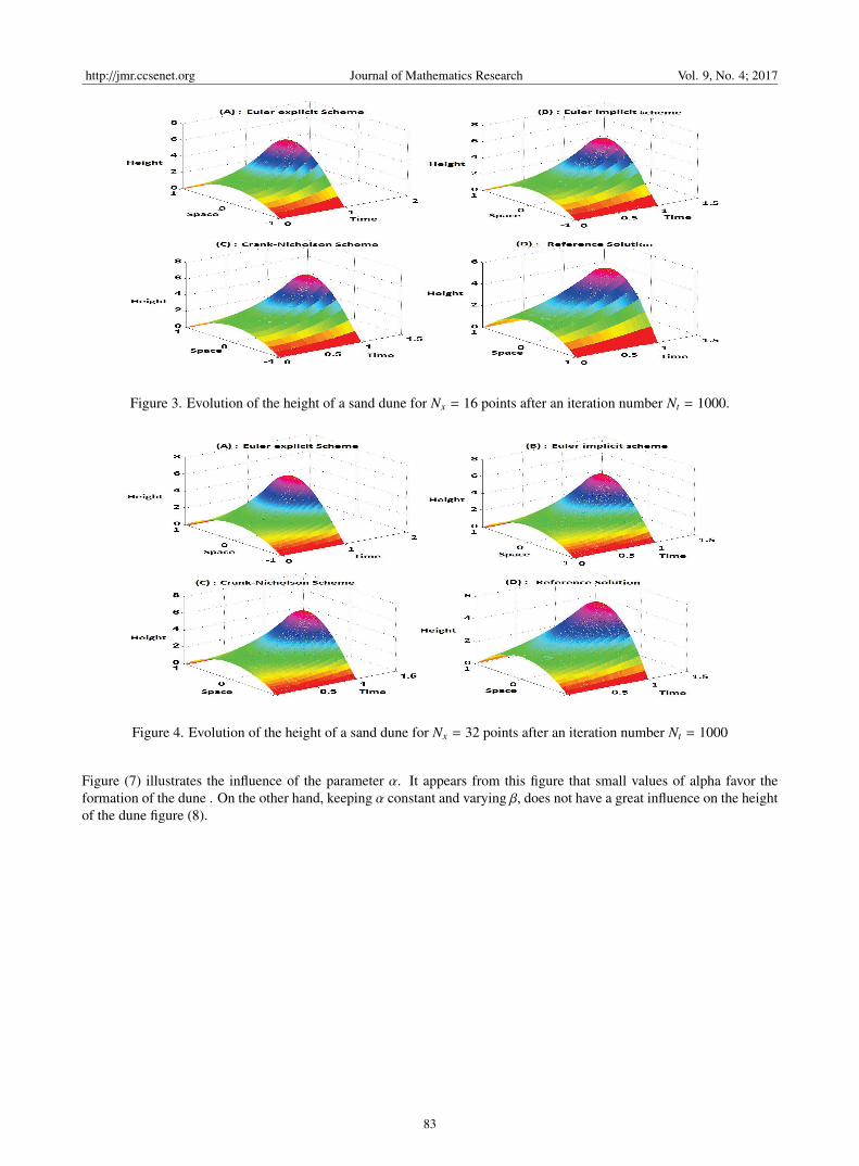
The above figures describe the evolution of a sand dune with different approximation schemes. For the starting form of thedune, we chose a polynomial bump of degree 2, h0 = 2(1− x2) with a maximum height of 2 m. Figures(1)-(6) illustrate theevolution of a sand dune for different values of discretization of the spatial and temporal domain. Through the differentsimulations we observe an increase in the height of the dune as a function of the temporal and spatial discretizationparameters. It should also be noted that for the implicit and Crank-Nicolson schemes the results are better when thenumber of discretization points increases while the explicit scheme produces a solution which deteriorates as the numberof points increases.The explicit Euler schemes gives solution that diverge when certain conditions are note satisfied.Thisdivergence is shown through figure (5A) which clearly show that the solution provide by the explicit method does notagree with the reference solution and those obtained by the two other methods when the discretization are ∆t = 0.001,∆x = 0.05. This scheme imposes a restriction on the discretization steps in time and space which is well known by theCourant, Friedrichs, Lewy condition (CFL). We can conclude that the Crank-Nicolson and implicit schemas are bettersuited for the approximation of our model problem than the explicit method.

Figures (7) and (8) give a simulation of the height of the sand dune as a function of the phenomena parameters α and β.

82


Figure 3. Evolution of the height of a sand dune for Nx = 16 points after an iteration number Nt = 1000.

Figure 4. Evolution of the height of a sand dune for Nx = 32 points after an iteration number Nt = 1000

Figure (7) illustrates the influence of the parameter α. It appears from this figure that small values of alpha favor theformation of the dune . On the other hand, keeping α constant and varying β, does not have a great influence on the heightof the dune figure (8).

83


Figure 5. Evolution of the height of a sand dune for Nx = 64points after an iteration number Nt = 1000.

Figure 6. Local crossplot of reference solution and solution of differente scheme at fixed time.

Figure 7. Evolution of a sand dune with β = 2, and D = 1 (of the fixed parameters) for different values of α

84


Figure 8. Evolution of a sand dune with α = 2, and D = 1 (fixed parameters) for different β values

5. Error Analysis

Different errors estimations are reported in following tables.

Table 1. Error estimation for 8 points and for ∆t∆(x)2 = 0.125

Time 40 50 60 70 80Explicit schema error 0.01 0.0096 0.0083 0.0069 0.0056Implicit schema error 0.029 0.027 0.025 0.023 0.021Crank-Nicholson shema error 0.21 0.020 0.018 0.016 0.015


Time 40 50 60 70 80Explicit schema error 0.4471×e−4 0.3832×e−4 0.3108×e−4 0.2324×e−4 0.1495×e−4

Implicit schema error 0.8831×e−4 0.8570×e−4 0.8134×e−4 0.7575×e−4 0.6922×e−4

Crank-Nicholson shema error 0.5924×e−4 0.5411×e−4 0.4783×e−4 0.4074×e−4 0.3305×e−4


Time 40 50 60 70 80Explicit schema error 0.1420×e−7 0.1557×e−7 0.1676×e−7 0.1780×e−7 0.1872×e−7

Implicit schema error 0. 2816×e−7 0.3101×e−7 0.3350×e−7 0.3570×e−7 0.3765×e−7



Time 40 50 60 70 80Explicit schema error 3.3924×e27 1.0268×e19 2.6938×e17 7.0747×e15 1.85×e12

Implicit schema error 0.1179×e−3 0.1082×e−3 0.0965×e−3 0.0840×e−3 0.0710×e−3



Time 40 50 60 70 80Explicit schema error 1.1764×e17 3.1×e15 8.8359×e13 2.5773×e10 7.6629×e8

Implicit schema error 0. 4720×e−7 0.5109×e−7 0.5436×e−7 0.5715×e−7 0.5956×e−7


85


The Tables 1−5 illustrate the approximation errors obtained by the different schemes for different numbers of discretizationpoints at a time T of evolution of the dune and a given value of the ration ∆t

∆(x)2 . It is constant that on all the tables, forall the schemes, for a fixed number of points, the error decreases as the iteration time increases. On the other hand, ananalysis of Tables 1 and 3 shows that over the same period of evolution of the dune, and for the same ratio ∆t

∆(x)2 , when thenumber of points of iteration is increased, the approximation becomes better. When the ratio ∆t

∆(x)2 is small in front of acondition CFL which is ∆t

∆(x)2 <1

2αD , the explicit Euler scheme gives a better approximation than the other schemes. On theother hand, when the ratio is greater than the CFL condition, the explicit Euler scheme explodes.The positive exponentsin tables 4 and 5 simply show that the error generated by the explicit Euler method tends to infinity which expresses thenonconvergence of the method and the explosion phenomenon of the given solution by explicit Euler method when theCFL condition is not satisfied. The implicit scheme and Crank-Nicholson always gives better approximations which isperfectly mathematical agreement of the stability performed above.Indeed, it has been shown that the implicit Euler andCrank schemes are unconditionally stable while the explicit Euler scheme is stable if the ratio ∆t

∆(x)2 is lower than the CFLcondition.

6. Conclusion

In this paper we have presented a simplified model of sand dune formation that we have approached by classical numericalmethods and we simulated this model. These simulations allowed us not only to choose the appropriate method for theanalysis of this model but above all to numerically determine the determining parameter in the formation of sand dunes.This parameter will enable us in a future work to control the movement of these dunes.

References

Andreotti, B., Claudin, P., & Douady, S. (2002). Selection of dunes shapes and velocities. Part 2: A two dimensionnalmodelling, 1-12. https://doi.org/10.1140/epjb/e2002-00236-4.

Bagnold, R. A. (1941). The physics of blown sand and desert dunes, Methuen, London.

Daniel, B. (2001). Phnomnes collectifs dans les matriaux granulaires. Ecoulements de surface et rarrangements internesdans des empilements modles, thse de doctorat, University Paris Sud - Paris XI.

Hersen, P. (2004). on the crescentic shape of barchan dunes. The European Physical Journal B-Condensed Matter andComplex Systems, 37(4), 507-514. https://doi.org/10.1104/epjb/e2004-00087-y.

Jackson, P., & Hunt, J. (1975). Turbulent wind flow over a low hill. Quarterly, Journal of the Royal MeteorologicalSociety, 101(430), 929-955. https://doi.org/10.1002/qj.49710143015.

Kroy, K., Sauermann, G., & Herrmann, H. J. (2002). Minimal model for sand dunes . Physical. Review E 66.https://doi.org/10.1103/PhyRevLett.88054301.

Matteo, P., Luca, F., & Fabio, N. (2011) Mathematical modelling for the evolution of aeolian dunes formed by a mixtureof sands: entrainment-deposition formulation. Communications in Applied and Industrial Mathematics, 1-21.https://doi.org/10.1685/journal.caim.000377.

Sauermann, G. (2001). Modeling of Wind Blown Sand and Desert Dunes PhD thesis, Universitat Stuttgart.

Schwammle, V., & Herrmann, H. (2004). Modelling transverse dunes, Earth Surface Processes and Landforms, 29(6),769-784. https://doi.org/10.1002/esp.1068.

Schwammle, V., & Herrmann, H. (2005). A model of barchan dunes including lateral shear stress. The European PhysicalJournal E: Soft Matter and Biological Physics, 16(1), 57-65. https://doi.org/10.1140/epje/e2005-00007-0.

STAM, J. M. T. (1997). On the modelling of two-dimensional aeolian dunes. International Association of Sedimentolo-gists, Sedimentology, 44, 127-141. https://doi.org/10.1111/j.1365-3091.1997.tb00428.X

Copyrights

Copyright for this article is retained by the author(s), with first publication rights granted to the journal.

This is an open-access article distributed under the terms and conditions of the Creative Commons Attribution license(http://creativecommons.org/licenses/by/4.0/).

86

Documents

Modeling and Numerical Simulation of Sand Dunes Formation · Journal of Mathematics Research; Vol. 9, No. 4; August 2017 ISSN 1916-9795 E-ISSN 1916-9809 Published by Canadian Center