Division of Solid Mechanics

ISRN LUTFD2/TFHF--04/5105--SE (1-80)

MODELING AND EXPERIMENTAL STUDIES OF PC/ABS AT LARGE DEFORMATIONS

Master’s Dissertation by

Henrik Persson and Kent Ådán

Supervisors Vijay Sharan, Sony Ericsson

Mathias Wallin, Div. of Solid Mechanics Paul Håkansson, Div. of Solid Mechanics Matti Ristinmaa, Div. of Solid Mechanics

Copyright © 2004 by Div. of Solid Mechanics, Sony Ericsson, Henrik Persson and Kent Ådán

Printed by KFS AB, Lund, Sweden.

For information, address: Division of Solid Mechanics, Lund University, Box 118, SE-221 00 Lund, Sweden.

Homepage: http://www.solid.lth.se

Preface This Master’s Thesis was done at the request of Sony Ericsson Mobile Communications AB and with supervision from the Division of Solid Mechanics, Lund University during the period of September 2003 to March 2004. The primary work has been done at Sony Ericsson Mobile in Lund. The material tests and computer simulations have been made at the University of Lund. The thesis was carried out in order to adapt an existing material model in ANSYS that de-scribe one of the thermoplastic materials that Sony Ericsson currently uses. During this period of time we have learned a lot about practical tests combined with advanced theoretical studies of material behaviour. The many issues we have faced have given many new aspects of the problems that an engineer deals with. There are lots of people who have helped us throughout this project. First we would like to express our gratitude towards Engineering Calculations Specialist Vijay Sharan, Sony Ericsson, Prof. Matti Ristinmaa, Solid Mechanics. Especially, we would like to thank Candidate for the doctorate Paul Håkansson and Dr. Mathias Wallin, Solid Mechanics for many valuable discussions and suggestions. We would also like to thank Senior Specialist, Tommy Sandevi, Sony Ericsson for sharing his knowledge of thermoplastic materials and Principal Librarian, Katarina Bulat, Sony Ericsson for her supply of relevant articles, without all this help, this thesis would have been difficult to accomplish. Finally, we would like to thank Customer Technical Field Support Elke Kaul, GE Plastics for all the material data he have had the trouble to provide us, Tool Maker Lars-Erik Persson, Alfa Laval for making some of the test specimens and Laboratory Technician Zivorad Zivkovic, LTH for calibrating the tensile test equipment. Lund, March 2004 Henrik Persson, Kent Ådán

Abstract This Master’s Thesis was done in collaboration with the division of solid Mechanics at University of Lund and Sony Ericsson Mobile Communications AB. The objective for the assignment was to adopt a material model that describes one of the thermoplastic materials that Sony Ericsson currently uses. This was done to, in a more accurate way than present, anticipate fault in the construction before starting the manufacturing process. In this Master’s Thesis, different kinds of rate-dependent constitutive models were investigated. The purpose was to find out what properties that can be simulated and what cannot. The focus of the investigation of material models was towards models that are implemented in ANSYS. After a strictly theoretical examine of suitable material models, tensile tests were performed in order to understand the qualitative behaviour of the thermoplastic material. Constant dis-placement rate tension tests were performed on all test specimens for comparison with the simulated tensile test results from finite element analysis. A displacement controlled applica-tion was chosen because of the critical necking phase. Due to the lack of test equipment that could measure the cross section area decrease, we had to find this area dependent stress-strain data by comparing simulated data with data from tensile tests. There are only two material models available in ANSYS that are suitable for modelling large strain rate-dependent plasticity, namely the Perzyna model or the Peirce model. Both of the models must be used in combination with isotropic hardening plasticity. The isotropic hardening plasticity is described by an input of a true stress-strain curve. Peirce model did not describe the thermoplastic material in a satisfying manner, hence this model was excluded. There are very limited ways of calibrating the constitutive models in ANSYS. To simulate the viscous behaviour of the investigated thermoplastic, the viscosity parameters must be adapted in the Perzyna model. All made tensile tests at the different strain rates were simulated in ANSYS with the selected parameters, until satisfying results were achieved. The Perzyna model describes the mechanical behaviour well, for the investigated strain rates. The overall test results show satisfactory agreement with the simulated results, with the only exception for static condition where the agreement between real tests and simulations were not totally satisfying in the softening region. This is due to the limitations in the plastic mate-rial model. Tensile tests, with ordinary test specimens are suitable for analyzing material behaviour. Un-fortunately this test technique can only describe material behaviour in one dimension. There-fore a verification test was needed, that could describe the whole stress field. This test was made in the same way as an ordinary tensile test process, but with a slightly modified test specimen. The simulated results showed a high agreement with the tensile test results. This is a proof of that the Perzyna model can describe more complicated geometries at a higher strain rate for the investigated PC/ABS plastic, more accurately, than with the presently used material model.

Contents 1 Introduction.......................................................................................................................................... 1

1.1 Presentation of Sony Ericsson Mobile Communications AB ....................................................... 1 1.2 Background to the assignment ...................................................................................................... 1 1.3 Objectives ..................................................................................................................................... 1 1.4 Restrictions ................................................................................................................................... 1

2 Presentation of thermoplastic materials............................................................................................. 3 2.1 History........................................................................................................................................... 3 2.2 The characteristics of the plastics ................................................................................................. 3

3 Introduction to large deformations .................................................................................................... 4 3.1 An introduction to Cartesian index notation and tensor algebra ................................................... 4 3.2 Description of motion of deformation........................................................................................... 5

3.2.1 Deformation gradient ........................................................................................................... 5 3.2.2 Strain tensors........................................................................................................................ 6 3.2.3 Stretch tensors...................................................................................................................... 8

3.3 Rate of deformation tensor............................................................................................................ 9 3.4 Stress tensors............................................................................................................................... 12

4 Constitutive models............................................................................................................................ 14 4.1 Material frame indifference......................................................................................................... 14 4.2 Elasticity at finite strain .............................................................................................................. 16

4.2.1 Hypo-elasticity................................................................................................................... 16 4.2.2 Hyper-elasticity.................................................................................................................. 17

4.3 Plasticity theory........................................................................................................................... 18 4.3.1 Yield criterion .................................................................................................................... 18 4.3.2 Hardening rule ................................................................................................................... 19 4.3.3 Flow rule ............................................................................................................................ 22

4.4 Hypo-elastic-plastic constitutive model ...................................................................................... 22 4.5 Rate-dependent plasticity ............................................................................................................ 23

4.5.1 Viscosity models................................................................................................................ 24 5 Material testing................................................................................................................................... 26

5.1 The stress-strain curve ................................................................................................................ 26 5.2 The plastic behaviour .................................................................................................................. 28 5.3 Data from the material supplier................................................................................................... 29 5.4 The tensile test ............................................................................................................................ 30

5.4.1 Test preparation ................................................................................................................. 30 5.4.2 Testing procedure............................................................................................................... 31 5.4.3 Results of tension tests....................................................................................................... 31

6 Calibration of the constitutive model ............................................................................................... 33 6.1 Numerical simulation of the uniaxial tensile testing of PC/ABS................................................ 34

6.1.1 Element type ...................................................................................................................... 34 6.1.2 Mesh................................................................................................................................... 35 6.1.3 Necking simulation ............................................................................................................ 35 6.1.4 Boundary conditions .......................................................................................................... 36

6.2 Modifying the input data............................................................................................................. 37 6.3 Determination of viscosity parameters........................................................................................ 39

6.3.1 The parameters mand γ ................................................................................................... 39 6.4 Results......................................................................................................................................... 41

7 Verification of the material model .................................................................................................... 48 7.1 Tensile test of plate with hole ..................................................................................................... 48 7.2 Simulation of test specimen with hole ........................................................................................ 49

7.2.1 Element type and mesh ...................................................................................................... 49 7.2.2 Loads and boundary conditions ......................................................................................... 49 7.2.3 Results................................................................................................................................ 50

8 Conclusions ......................................................................................................................................... 55 9 References ........................................................................................................................................... 56

1

1 Introduction

1.1 Presentation of Sony Ericsson Mobile Communications AB In 2001 the company Sony Ericsson Mobile Communications AB was established by tele-communications leader Ericsson and Sony Corporation. The company is equally owned by Ericsson and Sony. Sony Ericsson is responsible for product research, development and design, as well as market-ing and sales, distribution and customer’s service. The company’s global corporate manage-ment is based in London. Approximately 3,500 employees are working around the world. The company’s President is Katsumi Ihara, and Executive Vice President is Jan Wäreby. The new company’s first joint product was announced in March 2002 and now has a complete portfolio covering all target groups. The combine strength of Sony and Ericsson, and its strong consumer-focused and application-led strategy, make the company a leading player in the mobile communications industry [21].

1.2 Background to the assignment The cellular telephone market is in an expanding phase. Nowadays consumers use the phone in many different environments and in a reckless way, influencing the demands on strength of the phone. Without taking this into account before the production, this may cause great ex-penditure and negatively impact the company’s reputation. Currently, a diverse collection of plastic materials are widely used for reduction of weight and manufacturing costs. By using FE calculations to predict the characteristics of the phone in an early phase many expensive errors can be avoided. Today there is no accurate material model used at Sony Ericsson that supports simulations of thermoplastic materials exposed to large deformations. The background for the assignment is therefore to investigate and find the most suitable constitutive model implemented in ANSYS that supports large deformation, for the thermo-plastic material Sony Ericsson presently uses.

1.3 Objectives In this Master’s Thesis, different kinds of constitutive models for thermoplastic materials were investigated. Currently Sony Ericsson uses a material model that is not satisfying regarding high strain rate applications. The objective of the project was to determine the properties of the thermoplastic materials, by performing material testing. The experimental results were adapted to an existing material model in ANSYS, with restrictions taking into account. The FE-simulations of a test specimen were compared with the result from real ten-sile tests.

1.4 Restrictions The analysis does not accommodate material characteristics pertaining to the thermal behav-iour of the materials or effects of creep. Short term time dependent properties of the specified thermoplastic material, were however considered for the adoption. There are a few material models available in ANSYS that may be suited for the specified thermoplastic. Unfortunately, the limited time in a Master’s Thesis does not allow implementing own derived models.

2

In this thesis the structure of the thermoplastic material is assumed to be isotropic before and after the material has been deformed, which may affect the accuracy of the result. Some parts in this thesis have been omitted due to the request for secrecy; this explains the normalized values on the axes for all represented graphs, throughout this work.

3

2 Presentation of thermoplastic materials

2.1 History The material in its natural manner has been known in China and Egypt for many thousand years. Still, this material should be taken as new and undeveloped in many aspects. As early as in the 19th century, the chemists learned how to make use of natural macro molecules and ennoble them into half synthetics plastics. The discovery of cellulose nitrate, in the 1860 was a breakthrough for the plastics [15]. In the beginning of 20th century L Baekeland discovered phenol and formaldehyde (Bakelite). After that followed, from the middle of 1920 polyester plastic and polystyrene, among others were discovered [15]. In the 1930s, there was an intensive research on polymers, mainly in Germany and USA. Following this successful research, acrylic plastic (Plexiglas) and polyamide (Nylon) made their entrance. Nylon made a breakthrough during the Second World War, when it replaced the more expensive silk parachutes [7]. In modern time, the development of plastic materials is undergoing rapid progress and new materials are continually introduced. The reason why plastics have been so widely used mainly depends on its low weight and low manufacturing costs.

2.2 The characteristics of the plastics Traditionally, plastics are divided into thermoplastics and thermosets. In the thermosets, molecule chains are transversally linked into a three dimensional network. The hardening process starts first after a heat treatment or after adding a setting agent. The hardening process is not reversible and the plastic is therefore not recyclable, as the thermoplastics are. Thermo-plastics, on the other hand, consist of long chains of monomers from the polymerization proc-ess. The common machining capability for this plastic is injection molding and extrusion. Both of the plastics mentioned above, are suitable for addition of filling material, which change the properties of the material radically. The addition substance can be pigment, elasti-cizer, armoring, external flame retardant among others. One of the thermoplastic materials that Sony Ericsson is currently using is PC/ABS, an amorphous polycarbonate and acrylonitrile-butadiene-styrene thermoplastic polymer blend. PC/ABS has many manufacturing advantages when it comes to injection molding and extrusion. It has excellent filling capability for long and complex parts, without influencing the mechanical properties significantly. The plastic has excellent ductility, also at sub zero temperatures and it has a good heat resistance. Other engineering features of PC/ABS are the impact toughness and the relative rigidity it gives the product [10]. Sony Ericsson mostly uses PC/ABS for the shell of cellular telephones. The shell among other parts of the cellular tele-phone is produced by injection molding.

4

3 Introduction to large deformations When the strain exceeds more than a few percent a theory for large strain and large rotation must be used, since the geometry has deformed to an extent where the geometry change can not be neglected. Many applications of thermoplastic materials are subjected to deformations that can not be approximated as small. To describe thermoplastic materials when subjected to large strain or/and large rotations, more advanced theory needs to be considered [3]. Tensor notation is often used in tensor algebra to rewrite complicated expressions in a very compact fashion. Throughout this Master’s Thesis only Cartesian tensors will be considered.

3.1 An introduction to Cartesian index notation and tensor algebra To more easily understand the mathematical expression used in this master thesis, an introduction of tensor algebra will follow. The described theory in chapter 3.1 is taken from [19], if nothing else is indicated. A first order tensor ia can be rewritten into a column matrix and be expressed as

[ ] 32,1,

3

2

1

oriwhereaaa

ai =

= (3.1)

In what follows, Latin indices, unless otherwise specified, assume the values 1, 2 or 3. There are some conventions in index notation that will be mentioned below. If the same index is repeated twice, it is called a dummy index and otherwise it is called a free index. An example of the summation convention is the product aibi 332211 babababa ii ++= (3.2) It should be pointed out that the same index can appear not more than twice, otherwise the choice of index has no influence. The second order tensor ijB can be expressed in matrix format as

[ ]

=

333231

232221

131211

BBBBBBBBB

Bij (3.3)

Kronecker delta ijδ which plays an essential role in index notation and tensor algebra is de-fined as

≠=

=jiifjiif

ij 01

δ (3.4)

5

Using the Kronecker delta and the summation convention the following can now be expressed ikjkij BB =δ (3.5) Tensors must behave in a certain manner when exposed of translations and rotations. The different grades of tensors used in this thesis, are defined as tensororderzerobb ′= (3.6) tensororderfirstxAx jjii ′= (3.7) tensorordersecondATAT kjlkliij ′= (3.8)

3.2 Description of motion of deformation

3.2.1 Deformation gradient The expressions in chapter 3.2, are if not stated otherwise, taken from [18]. The loads acting on a body, makes it move from one position to another. This motion can be defined by studying a position vector in the deformed and undeformed configuration. At time 0=t , be-fore any motion, the position vector of a particle is described by the coordinates iX in the undeformed configuration. The position of the particle in the deformed configuration at time t is described by the position vector ix , see Figure 3.1.

The material deformation gradient maps a material point from the undeformed configuration into the deformed configuration and can be expressed as [16]

j

iij X

xF∂∂

= (3.9)

Figure 3.1: The undeformed and deformed configuration.

ix

iX

6

A conversion between jdX and idx can now easily be made jijijiji dxFdXordXFdx 1−== (3.10) which describes how the relative position vector jdX in the undeformed configuration has transformed to the position vector idx in the deformed configuration. The deformation gradient ijF contains information of the volume change, the rotation and the shape change of the deformed body. The volume change can be expressed as

ijFdVdVJ det

0

== (3.11)

where 0V is the original volume in the undeformed configuration and V is the current volume in the deformed configuration. The determinant J of the second order tensor ijF is called the Jacobian. The determinant of the tensor is an invariant, i.e. independent of the chosen coordinate sys-tem. If 1=J for all iX , the volume of the deformed and undeformed configuration are identi-cal and the deformation is said to be isochoric.

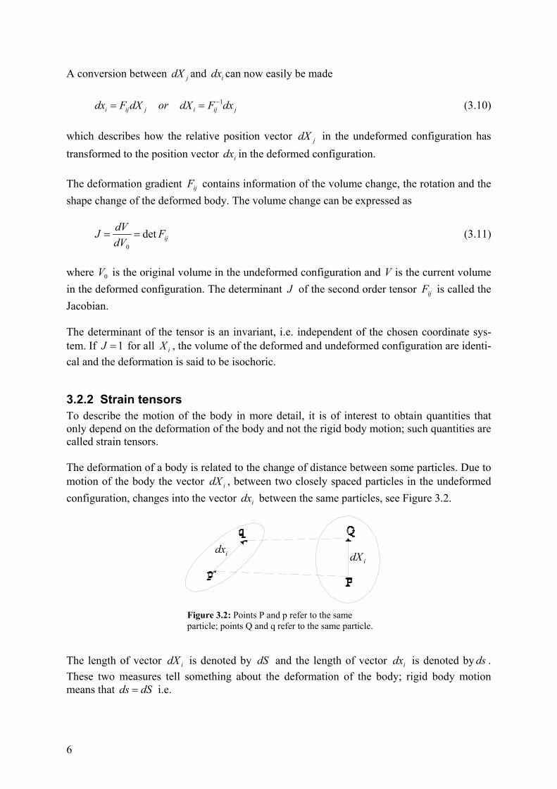
3.2.2 Strain tensors To describe the motion of the body in more detail, it is of interest to obtain quantities that only depend on the deformation of the body and not the rigid body motion; such quantities are called strain tensors. The deformation of a body is related to the change of distance between some particles. Due to motion of the body the vector idX , between two closely spaced particles in the undeformed configuration, changes into the vector idx between the same particles, see Figure 3.2.

The length of vector idX is denoted by dS and the length of vector idx is denoted by ds . These two measures tell something about the deformation of the body; rigid body motion means that dSds = i.e.

Figure 3.2: Points P and p refer to the same particle; points Q and q refer to the same particle.

idxidX

7

iiii dxdxdsdXdXdS == 22 ; (3.12) According to (3.10a), it follows that kjkj dXCdXds =2 (3.13) where

ikijk

i

j

ijk FF

Xx

XxC =

∂∂

∂∂

= (3.14)

The tensor ijC is termed the right Cauchy-Green deformation tensor and, moreover, it is noted that it is symmetric, i.e. kjjk CC = . A comparison of the lengths ds and dS is interesting in order to characterize the deforma-tion, with (3.12) and (3.13) it follows that jiji dXEdXdSds 222 =− (3.15) where

( )

−

∂∂

∂∂

=−=−= ijj

k

i

kijkjkiijijij X

xXxFFCE δδδ

21

21)(

21 (3.16)

is termed the Lagrangian strain tensor. In (3.16), the derivatives are taken with respect to iX , but it is also possible to obtain an expression for 22 dSds − , which involves derivatives with respect to ix . Insertion of (3.10b) into (3.12a) yields kjkj dxcdxdS =2 (3.17) where

k

i

j

ijk x

XxXc

∂∂

∂∂

= (3.18)

is termed Cauchy’s deformation tensor. The left Cauchy-Green deformation tensor is introduced as jkikijij FFcb == −1 (3.19)

8

3.2.3 Stretch tensors Another measurement of deformation of a body is the elongation or shortening of the distance between two close particles. Such a measure is provided by the so-called stretch.

dSds

=Λ (3.20)

where dS and ds have been defined earlier. To relate the stretch to the different deformation measures, the unit vector iN , in the direction of idX is introduced

dSdXN i

i = (3.21)

From (3.13), (3.20) and (3.21) it appears that jiji NCN=Λ2 (3.22) As seen in (3.22) the right Cauchy-Green deformation tensor is related to the square of the stretchΛ , therefore it is of interest to seek a deformation tensor which is linear in the stretch. Therefore the following expression is introduced ijij CU = (3.23) This tensor ijU is named the right stretch tensor. In the same manner using the left Cauchy-Green deformation tensor an analogous left stretch tensor can be defined as ijij bV = (3.24)

The polar decomposition theorem of Cauchy will be used below. It states that there exists two unique symmetric positive definite tensors ijU and ijV , the right and left stretch tensor, and an orthogonal tensor ijR such that kjikijkjikij RVForURF == (3.25) where ijR is the rotation tensor.

9

3.3 Rate of deformation tensor From (3.16) the Lagrangian strain tensor ijE is introduced and it has been shown that this ten-sor provides a complete description of the deformation of the body using the material de-scription, independent of rigid body motions. In some cases it is not the total change of deformation that is of importance, but rather the time rate with which these changes occur. When the constitutive equations are formulated in rate form like elasto-plasticity this situation arises. Therefore it is necessary to establish a ten-sor, which describes the rate with which deformation occurs. The theory throughout chapter 3.3 is taken from [18], if nothing else is indicated. Once again consider the length ds of the vector idx connecting two neighbouring particles in the deformed configuration, see Figure 3.2. This length is given by (3.12b). The material de-rivative of this expression gives

( ) ( )DtdxDdx

DtdsDds i

i= (3.26)

If ijF is expressed in material coordinates, i.e. ),( tXFF kijij = , the material derivative of (3.10a) then gives

( ) ( )DtdXD

FdXDt

DFDtdxD j

ijjiji += (3.27)

The vector jdX is independent of time, so the expression above can be reduced to

( )j

iji dXDt

DFDtdxD

= (3.28)

To evaluate the term DtDFij / , the material coordinates are adopted and it follows that

( ) ( )j

iki

jj

kiijij

Xv

ttXx

XXtXx

ttF

DtDF

∂∂

=

∂∂

∂∂

=

∂∂

∂∂

=∂

∂=

,, (3.29)

where (3.26) was used. This implies that (3.28) can be rewritten as

( )j

j

ii dXXv

DtdxD

∂∂

= (3.30)

If the velocity is expressed in terms of Eulerian coordinates, i.e. ( )txvv kii ,= , it follows that

kjk

i

j

k

k

i

j

i Fxv

Xx

xv

Xv

∂∂

=∂∂

∂∂

=∂∂ (3.31)

10

(3.30) then takes the form

( )jkj

k

ii dXFxv

DtdxD

∂∂

= (3.32)

which with (3.10a) becomes

( )k

k

ii dxxv

DtdxD

∂∂

= (3.33)

The spatial velocity gradient ijL is defined by

j

iij x

vL∂∂

= (3.34)

Then (3.33) can be written as

( )jij

i dxLDtdxD

= (3.35)

By introducing (3.35) into (3.26), it follows that

jiji dxLdxDtdsDds =

)( (3.36)

The unit vector in direction idx is given by dsdxn ii /= , which allows (3.36) to be written as

jiji nLnDtdsD

ds=

)(1 (3.37)

To rewrite this expression recall (3.20). It follows that

Λ

Λ=

Λ=

dsDtDdS

DtD

DtdsD )( (3.38)

Insertion into (3.37) gives

jiji nLnDtD

=Λ

Λ1 (3.39)

It appears that the material derivative of the stretch in the direction given by the unit vector in in the deformed configuration is related to the spatial velocity gradient ijL .

11

It is always possible to split ijL into a symmetric part ijD and an unsymmetrical part

ijW according to ijijij WDL += (3.40) where

tensorndeformatioofratexv

xvD

i

j

j

iij

∂

∂+

∂∂

=21 (3.41)

and

tensorspinxv

xvW

i

j

j

iij

∂

∂−

∂∂

=21 (3.42)

Now it is possible to establish the relation between the rate of deformation tensor ijD and the

material derivative ijE& of the Lagrangian strain. Next, (3.16) gives

( )kjkikjkiij FFFFE &&& +=21 (3.43)

In order to determine the quantity kjF& , (3.29), (3.31) and (3.34) are used to give

kjikkjk

i

j

iij FLF

xv

XvF =

∂∂

=∂∂

=& (3.44)

This expression together with (3.43) and (3.40) gives the sought relation ljklikij FDFE =& (3.45)

12

3.4 Stress tensors The expressions in this section are if not stated otherwise, taken from [18]. To establish the equations of motion, consider a body in its deformed configuration and make a section throughout the particle P. The normal in to the section is directed outwards of the body, cf. Figure 3.3.

On the incremental area dA surrounding the particle, the incremental force idP acts and the traction tensor it is then defined as

dAdPt i

i = (3.46)

If another section trough the same particle is taken, a different traction tensor will in general be obtained. Therefore, the traction tensor is a function of the direction jn , i.e. )( jii ntt = (3.47) If a direction parallel with one of the ix -axis is chosen, a certain traction it tensor is obtained. Consequently there exists three certain traction tensors, one for each ix -axis. This traction tensor can be expressed as

[ ]

=

3

2

1

i

i

i

itσσσ

(3.48)

There are several different stress tensors. The stress tensor, which represents the true stress, is called Cauchy stress tensor ijσ and is defined as

[ ]

=

=

333231

232221

131211

3

2

1

σσσσσσσσσ

σT

T

T

ij

ttt

(3.49)

Figure 3.3: Force dPi and area dA with outer unit normal vector ni.

in

idP

13

Two other stress tensors was introduced by Piola in 1833 and by Kirchhoff in 1852, where the first Piola-Kirchhoff stress tensor is defined as

k

jikij x

XJP

∂

∂= σ (3.50)

and the second Piola-Kirchhoff stress is defined as

j

lij

i

kkl x

XxXJS

∂∂

∂∂

= σ (3.51)

The first Piola-Kirchhoff tensor is unsymmetric and the second Piola-Kirchhoff tensor is symmetric. Another stress tensor is the Kirchhoff’s stress tensor which is defined as ijij Jστ = (3.52)

14

4 Constitutive models

4.1 Material frame indifference One of the requirements of the constitutive relations are that they must be coordinate invari-ant, i.e. if a constitutive relation holds in one coordinate system, it must hold in any other co-ordinate system. This requirement is fulfilled, when the constitutive relation is formulated in tensor quantities. Unfortunately the coordinate invariance is not enough, since it is also possible to change frame. Therefore the principle of frame indifference must be fulfilled as well, i.e. a function valid in one frame must be valid in all frames. In constitutive modelling and especially within plasticity theory, an introduction of the time-rate of the stress tensor is of interest. It is often found that the material derivate of an objective stress tensor is not always objective. An objective tensor must transform in a similar manner when the frame is changed as when the coordinate system is changed. To demonstrate this, the objective Cauchy stress tensor will be investigated ljklkiij QQ *σσ = and jlklikij QQ σσ =* (4.1) where ijQ describe a rigid body rotation. Now taking the material derivate of (4.1)

Dt

DQQQ

DtDQQ

DtDQ

DtD jl

klikjlkl

ikjlklikij σσσ

σ++=

*

(4.2)

It is evident that the tensor quantity DtD klσ is not objective. To obtain a valid objective stress rate, (3.40) is useful. The spatial velocity gradient can be expressed as

jlklikjkik

ij QLQQDt

DQL +=* (4.3)

and the expression of the rate-of-deformation as an objective tensor becomes jlklikij QDQD =* (4.4) Now the spin tensor (3.40) with (4.3) and (4.4) can be expressed as

jkik

jlklikij QDt

DQQWQW +=* (4.5)

Use of (4.2) and (4.5) gives

( ) ( )jmmljmmlklikljkl

ikjmlmklikklikij QWWQQQ

DtDQQWQQW

DtD

−++−= ***

σσσσ

(4.6)

15

this with (4.1) may be written as

jllmkmmlkmkl

ikjkikkjikij

QWWDt

DQWW

Dt

D

−−=−− σσ

σσσ

σ****

*

(4.7)

It appears that one can define following objective quantity from (4.7)

jkikkjikijJ

ij WWDt

Dσσ

σσ −−=∇ (4.8)

This expression is commonly known as the Jaumann rate of the Cauchy stress. Now the mate-rial derivate of Cauchy stress consists of two parts: the rate of change due to material re-sponse, which is reflected in the objective rate, and the change of stress due to rotation, which corresponds to the two last terms in (4.8). To prove that frame indifference is not only a mathematical problem, a realistic example will follow. Consider a bar that is initially loaded with a constant stress of 0σ . An observer that is riding with the body during a rotation (rigid body motion) of a bar in time will not observe any difference in stress, the initial value remains, Figure 4.1.

Since no deformation has occurred during the rotation, the rate-of-deformation ijD , equals zero, which is a correct assumption, but undecidedly leads to that 0=DtD ijσ which is in-correct see (4.2). The components of Cauchy stress in a fixed coordinate system will change during the rotation, so the material derivative of the stress must be nonzero. Obviously, something is missing in equation (4.2) since it does not support rigid-body-motions. The material rotation can be accounted for an objective rate of the stress tensor or often called a frame-invariant rate. There exist several objective rates, some more commonly are Truesdell-rate and Green-Naghdi-rate among others, but throughout this work all derivations are based on the Jaumann-rate.

Figure 4.1: Rotation of a bar under initial stress.

0σ 0σ

0,0 == yx σσσ 0,0 == xy σσσ

16

4.2 Elasticity at finite strain

4.2.1 Hypo-elasticity Hypo-elastic laws are used primarily for representing the elastic response in elasto-plastic material laws, where the elastic deformations are small. The most common elasto-plastic constitutive models that are implemented into conventional FE-programs are based upon Hypo-elasticity. The theory presented in chapter 4.2.1 and 4.2.2 is taken from [6], if nothing else is indicated. Hypo-elastic material laws relate the rate of stress to the rate of deformation. A general ex-pression of Hypo-elasticity is given by ( )klklijij Dg ,σσ =∇ (4.9) where ∇

ijσ represents any objective rate of the Cauchy stress tensor. The function ijg must also be an objective function of the stress and rate-of-deformation. Several of the Hypo-elastic constitutive relations can be expressed as linear relations between the objective measure of stress and the rate-of-deformation e

klijklJ

ij DC=∇σ (4.10) where J

ij∇σ is the Jaumann rate of Cauchy stress, e

klD is the elastic part of (3.41) and ijklC is the fourth-order elastic-moduli-tensor. This tensor can be expressed for an isotropic condition as ( )jkiljlikklijijklC δδδδµδλδ ++= (4.11) where λ and µ are the Lames constants. With a hypo-elastic formulation an undesired effect arises during a large elastic strain appli-cation. The strain energy is not necessarily conserved, i.e. the work done in a closed elastic deformation path is not necessarily zero, Figure 4.2.

Figure 4.2: Closed deformation path in a four step illustration.

17

4.2.2 Hyper-elasticity Hyper-elastic or often called Green elastic materials provide a natural frame-work for frame-invariant formulation [6], the frame indifference restrictions are trivially fullfilled if proper deformation measures are employed. Hyper-elasticity is a good model for non-linear elasticity, since the drawbacks of hypo-elasticity are avoided. Following expressions are taken from [18]. The second Piola-Kirchoff stress tensor, ijS , and the rate of Lagrangian strain tensor, ijE& , are conjugated quantities and therefore the strain-energy per unit reference volume can be ex-pressed as

( ) ( ) ij

E

klijij EdESEWij ~~

0∫= (4.12)

The notation ijE~ indicates that it is an integration variable. From (4.12) an energy increment can be expressed as ijijdESdW = (4.13) The energy increment can also be expressed as

ijij

dEEWdW∂∂

= (4.14)

With (4.13) and (4.14) the following expression holds

( )ijij

ij EWWwhereEWS =∂∂

= (4.15)

It appears that the strain energy W serves as a potential-function for the stresses. Choosing, for instance

klijklij ELEW21

= (4.16)

where ijklL is the positive definite constant stiffness tensor, results in the following simple hyper-elastic model klijklij ELS = (4.17)

18

4.3 Plasticity theory Plasticity theory provides a mathematical relationship that characterizes the elasto-plastic response of materials. There are three ingredients in plasticity theory [3]: the yield criterion, hardening rule and the flow rule. The theory throughout chapter 4.3 is taken from [19], if nothing else is indicated.

4.3.1 Yield criterion The yield criterion determines the stress level at which yielding is initiated. It is convenient to define a scalar function ,F as the yield criterion. If it is assumed that the material is isotropic, it does not have any preferred directions. Therefore, the initial yield surface can be expressed in terms of principal stresses [11] 0),,()( 321 === σσσσ FFF ij (4.18) This can also be expressed in terms of the invariants of the stress tensor as [11] 0),,( 321 == JJJFF (4.19) where 21, JJ and 3J are the invariants of the stress tensor and are defined by

kijkijjiijii sssJssJsJ31;

21; 321 === (4.20)

where ijs is the deviatoric stress tensor defined by

ijkkijijs δσσ31

−= (4.21)

Since the yield surface in general varies with the increase of plastic strains, it is possible to express the current yield surface by ,..2,10),( == ασ αKf ij (4.22) where the so-called hardening parameters αK are introduced. That characterizes the way in which the current yield surface changes its size, shape and position with plastic loading. The number of hardening parameters is unknown at the moment but as indicated; it is per-mitted to have more than one. The type of the hardening parameters may be scalars or higher-order tensors. Initially the hardening parameter is set to zero, this means that the current yield surface coincides with the initial yield surface. The choice of hardening parameters therefore implies a choice of hard-ening rule.

19

The hardening parameters αK vary with the plastic loading. To model this, it is assumed that there exist some internal variables that are used to memorize the plastic loading history. In analogy with the notation above, let βκ denote the internal variables =βκ internal variables ...)2,1( =β (4.23) initially0=βκ Because the internal variables memorize the plastic loading history, they are zero before any plasticity is initiated. Since the internal variables βκ characterize the elastic-plastic material, the hardening parameter αK depend on the internal variables βκ )( βαα κKK = (4.24)

4.3.2 Hardening rule The hardening rule describes the changing of the yield surface with increasing yielding. Three common hardening rules are: perfectly plastic, isotropic hardening and kinematic hardening. Thermoplastic materials often experience hardening during plastic straining. If a material is assumed not to experience hardening during plastic straining, the yield surface is unaffected by the plastic deformations, then it is called perfectly plastic [11]. Yield criteria for this type of material can be expressed with (4.22) as 0)()0,( == ijij Ff σσ (4.25) During plastic straining the shape, size, and orientation of the yield surface remain unchanged as shown in Figure 4.3.

The initial yield surface 0f is often defined as the locus of stress states when the first yielding occurs shown in Figure 4.3, inside the surface the stresses are elastic and the material behaves elastically. If an initially isotropic material hardens isotropically, the yield condition can be expressed as 0)(),( =−= αα σσ KFKf ijij (4.26)

Figure 4.3: Perfectly plastic.

20

In other words, as hardening occurs, the value of )( βα κK and the size of the yield surface changes with the development of plastic strains, shown in Figure 4.4. This event, will not affect the shape or orientation.

In mathematical terms, hardening is obtained by letting the function )( βα κK in (4.26) in-crease with increasing plastic deformation. If the function )( βα κK at some stage decreases with increasing plastic deformation then the yield surface shrinks in size corresponding to softening plasticity. As illustrated in Figure 4.5, if the loading is reversed from point A where yσσ = , the iso-tropic hardening model will predict elastic unloading until point B is reached. The isotropic hardening model predicts the same yield stress in tension and in compression. For some mate-rials, experimental results show that point B, where plastic effects again are encountered, occurs much earlier than predicted. This effect is called the Bauschinger effect.

Figure 4.4: Isotropic hardening.

Figure 4.5: Isotropic hardening.

yσ

0yσKy +0σ

Ky +0σ

yσ−

21

A way to approximate the Bauschinger effect is to assume that the difference between the two yield points is the value of 02 yσ , cf. Figure 4.6. This approximation of hardening is called kinematic hardening.

The idea of kinematic hardening is that the shape and size of the yield surface remain the same but the yield surface can translate in the direction of the plastic strain increment in the stress space, Figure 4.7.

During plastic deformations the yield surface can be expressed as 0)(),( =−= ijijij FKf ασσ α (4.27) where the hardening parameter in terms of the tensor ijα represents total translation of the yield surface. A more general hardening is obtained if the two models are combined into mixed hardening, i.e. both the size and the position of the yield surface are allowed to change.

Figure 4.7: Kinematic hardening.

Figure 4.6: Kinematic hardening.

0yσ0yσ

0yσ

22

4.3.3 Flow rule When the state of stress reaches the yield surface f , the material undergoes plastic deforma-tion; this is also called plastic flow [11], which is defined through a flow rule. The flow rule determines the direction of plastic straining and can be given as [3]

ij

pij

QDσ

λ∂∂

= & (4.28)

where p

ijD is the plastic part of (3.41) and λ& is the plastic multiplier, which determines the amount of plastic straining.Q is the plastic potential function which determines the direction of plastic flow direction. If Q is the yield function, the flow rule is referred to as an associative flow rule of plasticity [11] and the plastic strains occur in a direction normal to the yield surface [3]. Many materials are best modelled when the yield surface f and the plastic potential function Q are different. In the same way as in the flow rule, it is possible to establish a flow rule for the internal vari-ables.

αα λκ

Κ∂∂

=Q&& (4.29)

4.4 Hypo-elastic-plastic constitutive model The elasto-plastic constitutive models that ANSYS uses today are based upon hypo-elastic-plastic models. This model is an extension of hypo-elasticity, described in chapter 4.2.1. Following expressions are taken from [6]. The modelling of plasticity for large strains often implies an additive split of the rate of defor-mation, ijD into an elastic part and a plastic part p

ijeijij DDD += (4.30)

With (4.10) and (4.30) the Jaumann-rate can be expressed as ( )p

klklelijklJ

ij DDC −=∇,σ (4.31)

If the elastic moduli, elijklC , , is assumed to be constant, it must be isotropic in order to satisfy the principle of material frame indifference. Now introducing one important feature for Jaumann-rate, that ( )ijfσ and ijσ is commute. This leads to the following relationships ( ) ( )klijklij ff σσ σσ = and ( ) ( ) J

klijklij ff ∇= σσ σσ & (4.32)

23

Using the consistency relation 0=f& from (4.22) with the relation (4.31), the plastic flow rela-tion (4.28), the evolution equation (4.29) and the relation (4.32) gives the consistency condition

( )

( ) ( ) tuelrstursK

klelijklij

rCQhQDCQ

,

,

σαα

σλ+−

=& (4.33)

where ijij fr σ∂∂= is the plastic flow direction and α

α Kfh ∂∂= is the flow direction for internal variables. For an associative flow rule ( ) ( )ijij fQ σσ = .

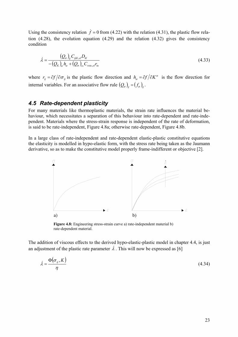
4.5 Rate-dependent plasticity For many materials like thermoplastic materials, the strain rate influences the material be-haviour, which necessitates a separation of this behaviour into rate-dependent and rate-inde-pendent. Materials where the stress-strain response is independent of the rate of deformation, is said to be rate-independent, Figure 4.8a; otherwise rate-dependent, Figure 4.8b. In a large class of rate-independent and rate-dependent elastic-plastic constitutive equations the elasticity is modelled in hypo-elastic form, with the stress rate being taken as the Jaumann derivative, so as to make the constitutive model properly frame-indifferent or objective [2].

The addition of viscous effects to the derived hypo-elastic-plastic model in chapter 4.4, is just an adjustment of the plastic rate parameter λ& . This will now be expressed as [6]

( )ησ

λKij ,Φ

=& (4.34)

b)a)

Figure 4.8: Engineering stress-strain curve a) rate-independent material b) rate-dependent material.

24

where ( )Kij ,σΦ is an overstress function and η is the viscosity. It shall be pointed out that the over stress function has the dimension of stress and can be considered as the driving force for the plastic strain [6]. To get a grip of how a rate-dependent model is composed, a one di-mensional rheological model will be considered, Figure 4.9.

The constant frictional stress is represented by yσ , η is the viscous constant and E is the elastic constant [14]. Thermoplastic materials in general have a material behaviour that com-bines all above described, Figure 4.9.

4.5.1 Viscosity models In this thesis, there was a limit of the available numbers of material models implemented in ANSYS, which support the plastic and viscous behaviour of PC/ABS. There are only three models in ANSYS that support visco-plasticity, Anand’s model, Peirce model and Perzyna model. Of those models mentioned above, there are only two material options available that are suitable for large strain rates, namely the Perzyna and the Peirce model. Both of these models must be combined with isotropic hardening. Another requirement is that the material model has to be able to describe the typical softening behaviour, cf. Figure 4.10

Figure 4.9: One dimensional rheological model.

0 0.1 0.2 0.3 0.4 0.5 0.6 0.7 0.8 0.9 10

20

40

60

80

100

120

True Strain

True

Stre

ss [M

Pa]

Figure 4.10: Softening behaviour.

Softening

1

1 )ln( 0LL

AF

25

One drawback for these models is that the strain rate effects are only active after plastic yielding has occurred [3] and it can not describe viscous effects during unloading. In a more detailed fashion, the models can be described as follows [3]. The visco-plastic flow rule is given as

ij

nyp

ijfDσσ

σγ

∂∂

−= 1

0

(4.35)

for Perzyna model and

ij

nyp

ijfDσσ

σγ

∂∂

−

= 1

0

(4.36)

for Peirce model, where yσ is the yield stress, 0σ is the static initial yield stress, n is a hardening parameter and γ is the viscosity parameter. The equivalent-plastic-strain rate is based on the visco-plastic flow rule as follows

pij

pij

peqv DD

32

=ε& = n

y

−1

0σσ

γ (4.37)

for Perzyna model and as

pij

pij

peqv DD

32

=ε& =

−

1

0

ny

σσ

γ (4.38)

for Peirce model.

26

5 Material testing The choice of material model is important and may not always be obvious. To understand the behaviour of the thermoplastic, it is necessary to perform material testing. A good way to evaluate material behaviour is to do tensile tests at different rates. This will, among other things, show viscous effects in the material. Some of the material properties are provided by the material supplier, but they need to be complemented with further material tests.

5.1 The stress-strain curve A uniaxial (one dimensional) stress-strain curve can be obtained from a tensile test. Often the applied load versus elongation is illustrated without any attention taken to the geometrical behaviour during loading. In order to extract meaningful information about the material be-haviour from the tensile tests, all effects of the specimen geometry needs to be eliminated. For materials where the strains are just a few percent, the cross section area decrease is not significant; in those cases the cross section area will be approximated to be constant. This is not the case for thermoplastic materials, where many load applications results in large strains and hence the cross section area can not be approximated as constant, cf. Figure 5.1. The following definitions are taken from [6].

Where the cross section area is approximated as constant, the mechanical response is often expressed in Engineering stress and Engineering strain. Define the stretch as

0L

L=λ (5.1)

where δ+= 0LL is the length of the gage section associated with elongation δ . The engineering strain is then defined as

10

0 −== λδεL

(5.2)

Figure 5.1: Geometrical behaviour during loading

27

The nominal or engineering stress is given by

0

0 AF

=σ (5.3)

where 0A is the original cross-sectional area. If the cross section area change is significant, true stress must be considered instead of the engineering stress.

AF

=σ (5.4)

where A is the current cross section area, i.e. not approximated to be constant any longer. The strain, ε , can be measured by integrating the change of unit current length. This measure of strain is called true strain or logarithmic strain.

( )∫ =

==

L

L LLdL

L0

lnln1

0

λε (5.5)

The time derivate of the logarithmic strain (5.5) will in one-dimensional case be equal to the rate of deformation.

11D==λλε&

& (5.6)

The nominal strain rate is defined as

0

0 Lδε&

& = (5.7)

Since

L&& =δ and λδ &

&&==

00 LL

L (5.8)

it follows that the nominal strain rate is equivalent to the rate of stretching, i.e. λε && = , in a one dimensional case. This relation is not true for general multiaxial states of deformation, unless the principal axes of the deformation are fixed.

28

5.2 The plastic behaviour Many polymers that undergo loading above the yield stress stretch uniformly for a few per-cent and then, instead of breaking, they fail by forming a neck. The neck may get steadily thinner until break, or it may stabilize at some point and then the shoulders travel along the specimen. In this case, the phenomenon is called cold-drawing [17] [22]. Necking is a geometrical behaviour, which typically starts before the softening on the engi-neering stress-strain curve. Furthermore strain will change the softening process into a hard-ening process until failure [1] [12] [13]. Another interesting feature of thermoplastic materials is that they show a different behaviour when they are exposed to compression compared to tension. When looking at Polycarbonate, PC, which is a component of PC/ABS, this effect is obvious, cf. Figure 5.2. The response in tension is significantly stiffer than in compression [4].

Figure 5.2: PC [4].

29

5.3 Data from the material supplier Figures 5.3 and 5.4 show data from the supplier of PC/ABS at different temperatures and load rates. Figure 5.3 show tensile tests at 23º C at different load rates. It has typical strain rate-dependence, since the load rate influence the load level for necking entry.

In Figure 5.4, a compression test has been made at different temperatures. Intuitive the mate-rial manage more load when cooled compared to a heated level. Under uniaxial compressive loading conditions, the underlying polymeric network chain structure is undergoing a planar orientation process which gives rise to the corresponding ob-served strain hardening behaviour. The necked region of the tensile specimen is being cold drawn resulting in a uniaxial state of orientation. Therefore, the observed engineering strain hardening in uniaxial tension distinctly differs from that obtained in uniaxial compression, giving different stress-strain curves [8] [5].

1

0 10 20 30 40 50 60 70 80 90 1000

10

20

30

40

50

60

70

80

90

100

110

10000 [%/s]1000 [%/s]100 [%/s]10 [%/s]0.8333 [%/s]

Figure 5.3: Tensile tests of PC/ABS at different load rates and a temperature of Co23 .

[ ]%0Lδ

1

0AF

Figure 5.4: Compression tests of PC/ABS at different temperatures.

0 10 20 30 40 50 60 700

10

20

30

40

50

60

70

80

90

100

110

23 deg C80 deg C-35 deg C

1

0AF

[ ]%0Lδ

30

5.4 The tensile test In order to accurately model the material behaviour, a reliable set of experimental data over an adequate range of strain rates is required. The true stress-strain testing of polymers is a formidable task due to the difficulty of conducting such tests to very large strains while maintaining a homogeneous state of deformation [4].

5.4.1 Test preparation All tensile tests were made at LTH with a tensile testing machine like the one in Figure 5.5, at normal temperature and pressure conditions.

The test specimen is injection-moulded and made of PC/ABS. The essential dimensions can be seen in Figure 5.6. 115 mm indicates the distance between the grips. Dimensions of the specimen follow the norm ISO 527-2/1A.

Figure 5.5: MTS tensile testing machine.

Figure 5.6: Test specimen ISO 527-2/1A.

31

5.4.2 Testing procedure Tensile tests with constant displacement rate were performed on all test specimens for com-parison with the simulated tensile test results from finite element analysis. A displacement controlled application was chosen because of the critical necking phase that would make the specimen collapse, if a load controlled application was chosen instead. The test equipment measures applied displacement versus obtained load. This data can not directly be transformed to true stress and true strain, since the cross section area decreases with the strain. Due to the lack of test equipment that could measure this area decrease, we had to find this in another way, which will be described in chapter 6. There is helpful equipment that can measure the cross section area, for example a CCD-cam-era. Even with this equipment this data is difficult to measure with accuracy, since the area decrease arises somewhere along the specimen during stretching and therefore one does not know where the area decrease takes place exactly. Unfortunately the material supplier could not support us with this data of true stress and true strain.

5.4.3 Results of tension tests Results of the tension tests made at different strain rates are shown in Figure 5.7. Near the maximum force, the specimen creates a neck and a very rapid decrease in cross section area appears. Once the neck stabilizes locally, drawing continues as material is pulled from the wider regions. During this time the load cell records very little increase in force.

Figure 5.7: Tensile test at different rates for PC/ABS.

0 10 20 30 40 50 60 70 800

500

1000

1500

2000

2500

Displacement [mm]

Forc

e [N

]

200 [mm/min]100 [mm/min]5 [mm/min]0.5 [mm/min]

F

[ ]mmδ

1

32

From the material supplier data, Figure 5.3, and from the tensile tests in Figure 5.7, it is obvi-ous that the material behaves differently when exposed to varying strain rate. This indicates that the material is rate-dependent, which must be considered when choosing the material model. To evaluate the yield stress of PC/ABS one needs to do further material tests, where the rate-dependent contribution is eliminated. Due to this a static tensile test was done, cf. Figure 5.8. Unloading this static curve at midway will identify if there exists any remaining deformation, at this load level.

Obviously there exists a remaining deformation at this load level, Figure 5.9. In metals an often used plastic limit is the so called RP0.2 limit, which occurs when 0.2% remaining plastic deformation exists after unloading. For materials like thermoplastics this entry is not so sharp and may be effects of the rate-dependence. This is the reason why an exact yield stress is hard to define for PC/ABS.

0 10 20 30 40 50 60 70 800

200

400

600

800

1000

1200

1400

1600

1800

2000

Displacement [mm]

Forc

e [N

]

Figure 5.8: PC/ABS loading at a rate of 0.5 mm/min

F

[ ]mmδ

0.8

0 0.2 0.4 0.6 0.8 1 1.2 1.4 1.6 1.8 20

200

400

600

800

1000

1200

Displacement [mm]

Forc

e [N

]

Figure 5.9: PC/ABS Unloading at a rate of 0.5 mm/min

[ ]mmδ

0.48

F

33

6 Calibration of the constitutive model Material models are mathematical descriptions of material behaviour. For the adoption of the material model, one needs to determine several material parameters therefore experimental data is needed. According to Figure 5.3 and 5.7, PC/ABS is showing rate-dependent effects. Due to lack of information, one does not know if the viscous effects exist in the elastic region. The isotropic hardening is in ANSYS described by an input of a true stress-strain curve like the one in Figure 6.1. Before the calibration will be described, the procedure of numerical simulations must be explained.

00

True Strain

True

Stre

ss

Figure 6.1: True stress versus true strain.

( )0ln LL

AF

34

6.1 Numerical simulation of the uniaxial tensile testing of PC/ABS

6.1.1 Element type All simulations in ANSYS made in this thesis are based upon the 3D-solid element, Solid185. This element has eight nodes, node I through P Figure 6.2, and each node has three degrees of freedom, UX, UY, UZ. This element supports orthotropic behaviour [3] Young’s modulus, zyx EEE ,, . Poisson’s ratio, zyx υυυ ,, or the shear angle, zyx γγγ ,, . Temperature dependence, zyx ααα ,, .

Other features that this element supports are plasticity, hyper-elasticity, creep, visco-plasticity, damping analysis and large strains [3].

Figure 6.2: Solid185

35

6.1.2 Mesh The simulated model of the tensile specimen represents the real one, with measurements according to Figure 5.6. Since there exist two planes of symmetry, only a quarter of the test specimen will be used, cf. Figure 6.3.

The use of symmetry planes reduces the simulation time noticeably. For many simulation applications, a 2-D model would be sufficient for Sony Ericsson. Unfortunately the simplifi-cation plane-stress, which could be an interesting alternative for simulations of cellular tele-phone shells, does not work for this model. The mesh, which consists of 2640 elements, was divided in five regions, regarding element size. This was done to more easily change element size in sensible regions, if convergence problems occur. Since there exist large strains and thereby the elements are exposed to large stretching, one needs a tight mesh to avoid highly disordered elements. This will increase the calculation time, but otherwise maintain a reasonable accuracy of the simulation results.

6.1.3 Necking simulation The simulated part has a necking behaviour in the same manner as a real test specimen. Since the narrowest width of the test specimen follows through over the whole test specimen, Figure 6.3a, a small imperfection was made to control the initial point of the necking. This imper-fection of the test specimen was introduced in form of a width decrease of 1 % at the centre of the specimen (the bottom of the mesh), Figure 6.3b.

Figure 6.3: Finite element model of a quarter of the tensile test specimen.

36

6.1.4 Boundary conditions The nodes along the x- and y-axis of symmetry are constrained to have no displacement in

yU and xU , respectively. The nodes located at the top of the specimen are constrained in zU and prescribed to move in the vertical direction yU , at a constant displacement rate corre-sponding to that applied in one of the actual experiments, cf. Figure 6.4.

Figure 6.4: Test specimen, boundary conditions.

∆

37

6.2 Modifying the input data Usually all calculations are based upon engineering data in terms of engineering stress and engineering strain. In large strain analysis, generally stress-strain input is in terms of true stress and true strain. In small strain applications, the area reduction effect is insignificant and it will therefore not affect the accuracy of the simulation results. From Figure 6.5, the curve with the slowest rate is considered as static in this thesis. This curve was also the base for the true stress-strain curve.

For small-strain regions of response, true strain and engineering strain are essentially identi-cal. There is no efficient way to convert engineering stress to true stress, therefore an initial guess; an assumption from [3] was used ( )engengtrue εσσ += 1 (6.1) This stress adaptation is valid only for incompressible plasticity. This is not the fact for the investigated thermoplastic where Poisson’s ratio is not constant throughout the yield point due to cavitations [9]. Expression (6.1) should not be used after softening has been initiated due to the area decreasing. The adaptation to true stress and true strain after necking was therefore only a qualitative guess based upon earlier work see Figure 5.2. The developed input data that is used throughout this thesis is illustrated in Figure 6.6.

Figure 6.5: Tensile tests made at different rates for PC/ABS.

0 10 20 30 40 50 60 70 800

500

1000

1500

2000

2500

Displacement [mm]

Forc

e [N

]

6900 [mm/min]690 [mm/min]200 [mm/min]100 [mm/min]57.5 [mm/min]5 [mm/min]0.5 [mm/min]

F

[ ]mmδ

1

38

Figure 6.6: Input data to ANSYS expressed in true stress and true strain.

0 0.1 0.2 0.3 0.4 0.5 0.6 0.7 0.8 0.9 10

20

40

60

80

100

120

True Strain

True

Stre

ss [M

Pa]

AF

( )0ln LL1

1

39

6.3 Determination of viscosity parameters Calibration of the rate-dependent behaviour, i.e. determination of the viscosity parameters, is an important aspect when simulating the behaviour of snaps or conducting simulations of drop tests, where the strain rates are high. Simulation programs, like ANSYS, require viscos-ity parameters to manage calculations at different strain rates.

6.3.1 The parameters m and γ The next step is to calibrate the parameters m and γ in a satisfying manner. Rearranging (4.37) gives the Perzyna equation

01 σγε

σ

+=

mineqv

y

& (6.2)

Corresponding equation for Peirce (4.38) is

01 σγε

σmin

eqvy

+=&

(6.3)

where: =yσ material yield stress

=ineqvε& equivalent plastic strain rate

== nm 1 strain rate hardening parameter

=γ material viscosity parameter =0σ static yield stress of material As γ approach ∞ , or m approach zero or in

eqvε& approach zero, the solution converges to the

static solution for Peirce. As γ approach ∞ , or ineqvε& approach zero, the solution for Perzyna

converges to the static solution. However, for this material option when m is very small (< 0.1), i.e. when a rate-independent model is approached, the solution shows difficulties in con-vergence [20]. To be able to find the parameters m (a value between 0 and 1) and γ (a value between 0 and ∞ ), it is first necessary to determine the material yield stress, static yield stress and equivalent plastic strain rate for as many tensile tests as possible. Finding the yield stress for different strain rates is not an easy task with the given data. The only way is to make a qualified guess. By looking at tensile tests, see Figure 6.5, the yield stress is determined after the initial estimated linear part. Figure 6.7 shows a comparison between Perzyna model (6.2) (dashed line) and determined yield stress as a function of strain rate (solid line).

40

The determined yield stresses are only an estimate which will affect the values of m and γ noticeably. Figure 6.8 shows a comparison between determined yield stress as a function of strain rate (solid line) and the Peirce equation (6.3) (dashed line).

It is not hard to see that no combination of m and γ will fit the Peirce model, so this model will be eliminated from further analysis.

70018.0

==

γm

Figure 6.8: Yield stress as a function of strain rate (solid line) compared with Peirce model (dashed line).

0 0.1 0.2 0.3 0.4 0.5 0.6 0.7 0.8 0.9 130

31

32

33

34

35

36

37

38

39

40

Strain rate [1/s]

Yie

ld s

tress

[Mpa

]

[ ]sL 10δ&

0AF

0σ

34 0σ

0 0.1 0.2 0.3 0.4 0.5 0.6 0.7 0.8 0.9 130

31

32

33

34

35

36

37

38

39

40

Strain rate [1/s]

Yie

ld s

tress

[Mpa

]

Figure 6.7: Yield stress as a function of strain rate (solid line) compared with Perzyna model (dashed line).

[ ]sL 10δ&0σ

0AF

34 0σ

41

Initially in the analysis, the Perzyna model with the chosen parameters of m andγ , was used, Figure 6.7. As mentioned above, these parameters only work as an initial estimation due to the difficulty in finding the yield stress. Tensile tests at different strain rates were simulated in ANSYS with the chosen parameters and compared with the real tests, Figure 6.5. If the results were not satisfying, new parameters were estimated and simulated for all strain rates in Figure 6.5 until an adequate result was achieved.

6.4 Results The tensile tests were made at seven different strain rates, Figure 6.5, and compared with simulations made under the same conditions, Figure 6.9, 6.11, 6.12, 6.13, 6.15, 6.16 and 6.17 A typical plastic behaviour is the softening that occurs. This effect appears due to molecular rearrangement in the material. Describing this effect mathematically in a material model is difficult but has been achieved in this thesis, cf. Figure 6.10, 6.14 and 6.18. Simulations were done up to 80% global strains of the test specimen, with satisfying results. Of course, one must be aware of the limit when failure occurs. The material model that has been investigated is a visco-plastic model. This material model describes the softening behaviour well, at an arbitrary rate. Figure 6.9, 6.11, 6.12, 6.13, 6.15, 6.16 and 6.17 show real tensile tests made in a tensile test machine, at different strain rates, compared with simulations of tensile tests made in ANSYS with the visco-plastic model. Since we were testing the real specimen to failure, the same was done in the simulation. Unfortunately one does not know when break occurs in the simulation program, since the mesh keeps on stretching without notice. This is one of the reasons why one needs to do real tests to verify the validity of the simulation results. The tensile specimen at Figure 6.10, 6.14 and 6.18 are scaled to fit in the same figure. This explains the differences in width of the tensile specimen.

42

The slowest tensile test was done at a displacement-rate of 0.5 mm/min, which was also the selected curve that was stated to be static, Figure 6.9. It is obvious that the material model with the chosen parameters of m and γ can not describe the softening acceptably for static conditions, Figure 6.9. This drawback occurs because the Perzyna model approaches isotropic hardening plasticity at slow strain rates. Isotropic hardening plasticity is not able to describe this softening in a satisfying manner.

Figure 6.10: Von Mises stress of PC/ABS at a rate of 0.5 mm/min. MaxU refers to global displacement.

Maxσ = 70.5 MPa 76.7 MPa 80.3 MPa 82.2 MPa 84.9 MPa

Minσ = 4.9 MPa 5.0 MPa 5.0 MPa 5.0 MPa 5.1 MPa

MaxU = 10.0 mm 20.0 mm 40.0 mm 60.0 mm 80.0 mm

Minσ

Maxσ

0 10 20 30 40 50 60 70 800

500

1000

1500

2000

2500

Displacement [mm]

Forc

e [N

]

Figure 6.9: A real test (solid line) of PC/ABS at a rate of 0.5 mm/min compared with simulation (dashed line).

[ ]mmδ

F

1

43

The static result which was not totally satisfying, Figure 6.9, will not be a limitation for the material model, since in practical applications, static conditions are rare. The typical area decreasing phenomenon for thermoplastic materials, the so called cold-drawing is illustrated in Figure 6.10.

Already at a rate of 5 mm/min, the Perzyna model, describes the softening well, Figure 6.11.

0 10 20 30 40 50 60 70 800

500

1000

1500

2000

2500

Displacement [mm]

Forc

e [N

]

Figure 6.12: A real test (solid line) of PC/ABS at a rate of 57.5 mm/min compared with simulation (dashed line).

1

[ ]mmδ

F

0 10 20 30 40 50 60 70 800

500

1000

1500

2000

2500

Displacement [mm]

Forc

e [N

]

Figure 6.11: A real test (solid line) of PC/ABS at a rate of 5 mm/min compared with simulation (dashed line).

[ ]mmδ

F

1

44

Figure 6.14: Von Mises stress of PC/ABS at a rate of 100 mm/min. MaxU refers to global displacement.

Maxσ = 68.2 MPa 83.7 MPa 92.6 MPa 97.9 MPa 102.0 MPa

Minσ = 5.6 MPa 5.6 MPa 5.6 MPa 5.6 MPa 5.6 MPa

MaxU = 10.0 mm 20.0 mm 40.0 mm 60.0 mm 80.0 mm

Minσ

Maxσ

0 10 20 30 40 50 60 70 800

500

1000

1500

2000

2500

Displacement [mm]

Forc

e [N

]

Figure 6.13: A real test (solid line) of PC/ABS at a rate of 100 mm/min compared with simulation (dashed line).

1

[ ]mmδ

F

45

0 10 20 30 40 50 60 70 800

500

1000

1500

2000

2500

Displacement [mm]

Forc

e [N

]

Figure 6.15: A real test (solid line) of PC/ABS at a rate of 200 mm/min compared with simulation (dashed line).

1

[ ]mmδ

F

[ ]mmδ

F

Figure 6.16: A real test (solid line) of PC/ABS at a rate of 690 mm/min compared with simulation (dashed line).

0 10 20 30 40 50 60 70 800

500

1000

1500

2000

2500

Displacement [mm]

Forc

e [N

]

1

[ ]mmδ

F

46

0 10 20 30 40 50 60 70 800

500

1000

1500

2000

2500

Displacement [mm]

Forc

e [N

]

Figure 6.17: A real test (solid line) of PC/ABS at a rate of 6900 mm/min compared with simulation (dashed line).

1

[ ]mmδ

F

Minσ

Maxσ

Maxσ = 63.4 MPa 84.8 MPa 101.0 MPa 111.0 MPa 118.9 MPa

Minσ = 6.9 MPa 6.5 MPa 6.5 MPa 6.5 MPa 6.5 MPa

MaxU = 10.0 mm 20.0 mm 40.0 mm 60.0 mm 80.0 mm

Figure 6.18: Von Mises stress of PC/ABS at a rate of 6900 mm/min. MaxU refers to global displacement.

Minσ

47

Overall the test results show very good agreement with the simulated results, except from the softening behaviour at static condition. It should be pointed out that all tensile tests, show scattering in the results, Figure 6.19 and 6.20, probably due to material imperfections. This spreading partly explains the divergence between the real tests and simulations, throughout. The slower tensile rates, shows a lower force level before the necking phenomenon initiates, compare Figure 6.9 with Figure 6.17, as mentioned earlier this indicates viscous effects. When comparing the size of the waist area in Figure 6.10, 6.14 and 6.18, it is evident that the strain rate affects the initiating of necking and the size of the waist area enlarges with in-creasing rate. Exactly what causes this behaviour is hard to describe without further material investigation.

Figure 6.19: The scattering in result. Tensile tests of PC/ABS at a rate of 0.5 mm/min.

0 2 4 6 8 10 12 140

200

400

600

800

1000

1200

1400

1600

1800

2000

Displacement [mm]

Forc

e [N

]

1

F

[ ]mmδ

0 10 20 30 40 50 60 70 800

500

1000

1500

2000

2500

Displacement [mm]

Forc

e [N

]

Figure 6.20: The scattering in result. Tensile tests of PC/ABS at a rate of 200 mm/min.

1

F

[ ]mmδ

48

7 Verification of the material model Tensile tests, with ordinary test specimens are a good way of analysing material behaviour. Unfortunately this test technique can only describe material behaviour in one dimension. Due to this verification tests, so called “specimen with a cylindrical hole”, were made to evaluate the whole stress field. This test follows the same test procedure as a normal tensile test but with the difference that now the test specimen has a cylindrical hole at the centre.

7.1 Tensile test of plate with hole A tensile test was made in the same manner as described in chapter 5.4. This test specimen has the same dimensions according to ISO 527-2/1A, Figure 5.6, with the only difference that it has a 3.2 mm milled cylindrical hole in its centre, Figure 7.2. The addition of the cylindrical hole will describe a multi-axial stress field. Four different tensile tests were made with increasing strain rates to failure, Figure 7.1.

Figure 7.1: Test specimen with cylindrical hole at different rates.

0 0.5 1 1.5 2 2.5 3 3.5 40

200

400

600

800

1000

1200

1400

1600

Displacement [mm]

Forc

e [N

]

50 [mm/min]10 [mm/min]5 [mm/min]0.5 [mm/min]

1

F

[ ]mmδ

49

7.2 Simulation of test specimen with hole

7.2.1 Element type and mesh In the same manner as described in chapter 6.1, a similar tensile test was simulated in ANSYS to verify the results of the tensile test of the specimen with a cylindrical hole, described in 7.1. The mesh of the modelled tensile test specimen is overall identical with the earlier tensile tests described in chapter 6.1, with exception from addition of a cylindrical hole, Figure 7.2. This extra hole gives an increase in number of elements, which are now 2784.

7.2.2 Loads and boundary conditions Since this test specimen is almost identical to the one earlier described in chapter 6, with exception from the cylindrical hole, the geometrical symmetry can be used. In the same man-ner as described in chapter 6.1 only a quarter of the test specimen was used for analysis. Regarding the boundary conditions, these are the same as earlier described, but now with a smaller final displacement yU at the top, Figure 6.4.

Figure 7.2: Test specimen with a cylindrical hole.

50

7.2.3 Results The results from the tensile tests on the specimen with cylindrical hole are compared with the simulation in the same manner as described in chapter 6.4. Since the simulation can not de-scribe the actual failure, one needs to be aware of the limit when failure occurs.

Minσ

0 0.5 1 1.5 2 2.5 3 3.5 40

200

400

600

800

1000

1200

1400

1600

Displacement [mm]

Forc

e [N

]

Figure 7.3: A real test of specimen with cylindrical hole (solid line) of PC/ABS at a rate of 0.5 mm/min compared with simulation (dashed line).

1

F

[ ]mmδ

Figure 7.4: Von Mises stress of PC/ABS at a rate of 0.5 mm/min. MaxU refers to global displacement.

Maxσ

Maxσ = 51.2 MPa 105 MPa 119 MPa

Minσ = 3.78 MPa 3.41 MPa 3.45 MPa

MaxU = 2.0 mm 3.0 mm 4.0 mm

Minσ

51

Figure 7.6: Von Mises stress of PC/ABS at a rate of 5 mm/min. MaxU refers to global displacement.

Minσ

Maxσ

Maxσ = 53.4 MPa 103 MPa 125 MPa

Minσ = 3.79 MPa 3.58 MPa 3.60 MPa

MaxU = 2.0 mm 3.0 mm 4.0 mm

0 0.5 1 1.5 2 2.5 3 3.5 40

200

400

600

800

1000

1200

1400

1600

Displacement [mm]

Forc

e [N

]

Figure 7.5: A real test of specimen with cylindrical hole (solid line) of PC/ABS at a rate of 5 mm/min compared with simulation (dashed line).

1

F

[ ]mmδ

52

Figure 7.8: Von Mises stress of PC/ABS at a rate of 10 mm/min. MaxU refers to global displacement.

Minσ

Maxσ

Maxσ = 54.3 MPa 102 MPa 127 MPa

Minσ = 3.80 MPa 3.66 MPa 3.66 MPa

MaxU = 2.0 mm 3.0 mm 4.0 mm

Figure 7.7: A real test of specimen with cylindrical hole (solid line) of PC/ABS at a rate of 10 mm/min compared with simulation (dashed line).

0 0.5 1 1.5 2 2.5 3 3.5 40

200

400

600

800

1000

1200

1400

1600

Displacement [mm]

Forc

e [N

]

F

[ ]mmδ

1

53

Figure 7.10: Von Mises stress of PC/ABS at a rate of 50 mm/min. MaxU refers to global displacement.

Minσ

Maxσ

Maxσ = 56.6 MPa 98.9 MPa 134 MPa

Minσ = 3.82 MPa 3.93 MPa 3.83 MPa

MaxU = 2.0 mm 3.0 mm 4.0 mm

0 0.5 1 1.5 2 2.5 3 3.5 40

200

400

600

800

1000

1200

1400

1600

Displacement [mm]

Forc

e [N

]

Figure 7.9: A real test of specimen with cylindrical hole (solid line) of PC/ABS at a rate of 50 mm/min compared with simulation (dashed line).

1

F

[ ]mmδ

54

The overall test results show very good agreement with the simulated results, Figure 7.3, 7.5, 7.7 and 7.9. Still there is a spreading in result due to material imperfections, which will affect the results of the test comparison overall. In the same way as in chapter 6, the lower tensile rates, show a lower force level before softening initiates, Figure 7.3, 7.5, 7.7 and 7.9. It is noticeable that the strain rate influencing the initiating of softening and the size of the waist area enlarges with increasing rate, Figure 7.4, 7.6, 7.8 and 7.10. Overall the Perzyna model seems to describe the whole stress field satisfactorily.

55

8 Conclusions The investigated plastic, PC/ABS, shows a highly viscous behaviour, i.e. highly rate-depend-ent. In large strain applications for materials where the cross section area changes, it is im-portant to use input data in terms of true stress and true strain, to maintain the accuracy. Use of engineering data of PC/ABS in simulation programs makes the results less reliable, par-ticularly after necking has been initiated. Data of true stress and true strain is not available either in the literature or from the material supplier. This data can be obtained by comparing simulations of tensile tests with real tensile tests. The only useful material models in ANSYS for large strain rates, is the visco-plastic model namely, the Perzyna model. This model requires identification of the two parameters γ and m to describe the visco-plas-tic behaviour. Due to the request for secrecy these parameters can not be published. The Perzyna model describes the softening behaviour well and global strains up to 80 % at analyzed strain rates. Overall the test results show satisfying agreement with the simulated results, with the only exception for static condition, where the agreement between real tests and simulations were not totally satisfying in the softening region. This drawback arises from the Perzyna model approaching isotropic hardening plasticity at slow strain rates. Isotropic hardening plasticity is not able to describe this softening in a satisfying manner. A uniaxial tensile test can only describe material behaviour in one dimension. Due to that, a verification tensile test using a specimen with a cylindrical hole was made. This test describes the whole stress field. The results are satisfying in all analyzed strain rates for Perzyna model.

56

9 References [1] Aleksey, D. D. (1999), A Constitutive Model in Viscoelastoplasticity of Glassy Polymers, Polymer, Vol. 40, pp. 3711-3727. [2] Anand L. and Lush A. M. and Weber G. G. and Zavaliangos A. (1990), An Objective Time-integration Procedure for Isotropic Rate-independent and Rate-dependent Elastic-plastic Constitutive Equations, International Journal of Plasticity, Vol. 6, pp. 701-744. [3] ANSYS, Inc (2000), Structural Analysis Guide, ANSYS Release 5.7, SAS IP, Inc, USA. [4] Arruda, E. M. and Boyce, M. C. (1990), An Experimental and Analytical Investigation of the Large Strain Compressive and Tensile Response of Glassy Polymers, Polymer Engineering and Science, Vol. 30, No. 20, pp. 1288-1298. [5] Arruda, E. M. and Boyce, M. C. and Jayachandran, R. (1994), The Large Strain Compression, Tension and Simple Shear of Polycarbonate, Polymer Engineering and Science, Vol. 34, No 9, pp. 716-725. [6] Belytschko, T. and Liu, K. W. and Moran, B. (2001), Nonlinear Finite Elements for Continua and Structures, John Wiley and Sons, Ltd, Baffins Lane, Chichester, ISBN 0-471-98773-5. [7] Bonniers Stora Lexikon på CD (2000), Bonnier Lexikon AB. [8] Boyce, M. C. and Arruda, E. M. (1990), An experimental and analytical investigation of the large strain compressive and tensile response of glassy polymers, Polymer Engineering and Science, Vol. 30, No 20, pp. 1288-98. [9] Brown and Bubeck and Buckley and Kraemer, Modes of deformation in rubber modified thermoplastics during tensile impact, Journal of Material Science. [10] Campus 4.1 (1999), GE Plastics Europe. [11] Chandrakant, S. D. and Hema, J. S. (1984), Constitutive Laws for Engineering Materials with Emphasis on Geologic Materials, Prentice-Hall, Inc., Englewood Cliffs, New Jersey. [12] Dally, J. W. and Mulc, A. (1973), Polycarbonate as a Model Material for Three-Dimensional Photoplasticity, Journal of Applied Mechanics, Vol. 40, No. 2, pp. 600-605. [13] Hadjiiossiph, C. and Theocaris, P. S. (1979), Strain-Analysis of Neck Formation and Propagation in Glassy Polymers, Engineering Fracture Mechanics, Vol. 12, No. 2, pp. 241-252. [14] Hughes, T. J. R. and Simo, J. C. (2000), Computantional Inelasticity, ISBN 0-387-97520-9, Springer-verlag New York, Inc. [15] Klason, C. and Kubát, J. (2001), Plaster Materialval och materialdata, Författarna och Industrilitteratur AB, Utgåva 5.

57

[16] Lundgren, E. (2003), Lectures notes, Division of Mechanics, University of Lund. [17] Miller, L. C. and Nimmer, R. P. (1984), Neck Propagation in Tensile Tests: A Study Using Rate-Independent, Strain Hardening Plasticity, Journal of Applied Mechanics, Vol. 51, pp. 759-765. [18] Ottosen, S. N. and Ristinmaa, M. (1996), Large strain plasticity and thermodynamics, Division of Solid Mechanics, University of Lund. [19] Ottosen, S. N. and Ristinmaa, M. (1999), The Mechanics of Constitutive Modelling, volume 1, Division of Solid Mechanics, University of Lund. [20] Owen, D. R. J. and Peric, D. (1992), A Model for Large Deformations of Elasto-Viscoplastic Solids at Finite Strains: Computational Issues, Finite Inelastic Deformations: Theory and Applications, Springer-Verlag, Berlin. [21] Sony Ericsson Mobile Communications AB (2004-03-29), About Us, http://www.sonyericsson.com/uk/ [22] Vincent, P. I. (1960), The Necking and Cold-Drawing of Rigid Plastics, Polymer, Vol. 1, No. 7.