Modeling and Control of Retarder using On/O Solenoid Valves572695/FULLTEXT01.pdf · Modeling and control of Retarder is a work provided by Scania as a part of the development and

Modeling and Control of Retarder usingOn/Off Solenoid Valves

VIDAR STEINSLAND

Masters’ Degree ProjectStockholm, Sweden April 2008

XR-EE-RT 2008:007

Abstract

The Retarder is one of the main components in Scania’s trucks’ brakingsystem and is used to brake down the truck and for maintaining a steadyspeed on descents. This Master’s Thesis aims to investigate if the currentsystem which uses a proportional valve to control the air pressure in theRetarder, can be replaced with two on/off solenoid valves and a pressurechamber to control the air pressure, which would result in a cheaper and morerobust system. By varying the air pressure, the braking torque in the truckcan be regulated. A model including electrical drives from a control unit,valves, pressure chamber and a regulating valve is derived. Using the modelas reference, a controller is designed and implemented to control the valves,and thereby the pressure. Based on experience from employees at Scania andformer research on on/off control of an Exhaust Gas Recirculation system, aregular PID-controller is used as the base in the control. A pulsing schemewhere the valves are activated separately is used to distribute the controlsignal to the two valves. Different ways of applying the control signal areinvestigated, whether the valves run digital, i.e. 0 % or 100 %, or continuouslyby varying the PWM signal. A boosting action using non-linear control, andprediction are investigated in order to improve the control performance insuch way that the required time response and robustness is obtained. Thecontroller is eventually tested and verified on the real system.

Acknowledgments

I would like to express profound gratitude to my advisor at Scania, M.Sc.Tomas Selling, for his invaluable support, perseverance, supervision and use-ful suggestions throughout this research work. His moral support and con-tinuous guidance enabled me to complete my work successfully. I am alsohighly thankful to my supervisor Hakan Hjalmarsson, Professor at the Schoolof Electrical Engineering, Royal Institute of Technology, for his valuable sug-gestions throughout this study.

I appreciate the kindness of Mr. Fredrik Straat for his suggestions and ad-vices concerning the Retarder control unit, and would specially thank Mr.Richard Riis for his assistance with the prototypes used for tests and exper-iments.

I am also thankful to Mr. Soren Aberg, who guided me about the directionof my thesis from the beginning, and assisted with practical experiments.Finally, I wish to express my appreciation to the rest of the members ofNEST at Scania, and friends and family that have supported me in doingthis thesis.

1

Contents

1 Introduction 91.1 Background . . . . . . . . . . . . . . . . . . . . . . . . . . . . 91.2 Thesis Objectives . . . . . . . . . . . . . . . . . . . . . . . . . 101.3 Functional Description . . . . . . . . . . . . . . . . . . . . . . 101.4 Actuation Requirements . . . . . . . . . . . . . . . . . . . . . 111.5 Notation . . . . . . . . . . . . . . . . . . . . . . . . . . . . . . 13

2 Retarder 152.1 Scania’s Retarder . . . . . . . . . . . . . . . . . . . . . . . . . 15

2.1.1 Retarder System Today . . . . . . . . . . . . . . . . . 152.1.2 Retarder System Using On/Off Solenoid Valves . . . . 16

2.2 Dead Volume . . . . . . . . . . . . . . . . . . . . . . . . . . . 162.3 Solenoid Valves . . . . . . . . . . . . . . . . . . . . . . . . . . 172.4 Equipment in Experiments . . . . . . . . . . . . . . . . . . . . 19

2.4.1 ECU . . . . . . . . . . . . . . . . . . . . . . . . . . . . 192.4.2 Prototypes . . . . . . . . . . . . . . . . . . . . . . . . . 202.4.3 Retarder . . . . . . . . . . . . . . . . . . . . . . . . . . 212.4.4 Pressure Sensor . . . . . . . . . . . . . . . . . . . . . . 212.4.5 Software . . . . . . . . . . . . . . . . . . . . . . . . . . 222.4.6 Oscilloscope . . . . . . . . . . . . . . . . . . . . . . . . 222.4.7 Multimeter . . . . . . . . . . . . . . . . . . . . . . . . 22

3 Modelling 233.1 System Description . . . . . . . . . . . . . . . . . . . . . . . . 243.2 ECU Model . . . . . . . . . . . . . . . . . . . . . . . . . . . . 253.3 Valve . . . . . . . . . . . . . . . . . . . . . . . . . . . . . . . . 26

3.3.1 Electrical Model . . . . . . . . . . . . . . . . . . . . . . 263.3.2 Magnetic Model . . . . . . . . . . . . . . . . . . . . . . 293.3.3 Mechanical Model . . . . . . . . . . . . . . . . . . . . . 293.3.4 Pneumatic Model . . . . . . . . . . . . . . . . . . . . . 31

3.4 Regulating Valve . . . . . . . . . . . . . . . . . . . . . . . . . 33

2

3.5 Model Summary . . . . . . . . . . . . . . . . . . . . . . . . . 35

4 Model Validation 374.1 Duty Cycle Limits . . . . . . . . . . . . . . . . . . . . . . . . 384.2 Prototype 1 . . . . . . . . . . . . . . . . . . . . . . . . . . . . 39

4.2.1 Filling Characteristics . . . . . . . . . . . . . . . . . . 404.2.2 Ventilation Characteristics . . . . . . . . . . . . . . . . 404.2.3 Friction . . . . . . . . . . . . . . . . . . . . . . . . . . 424.2.4 Validation . . . . . . . . . . . . . . . . . . . . . . . . . 42

4.3 Prototype 2 . . . . . . . . . . . . . . . . . . . . . . . . . . . . 474.3.1 Filling Characteristics . . . . . . . . . . . . . . . . . . 484.3.2 Ventilation Characteristics . . . . . . . . . . . . . . . . 494.3.3 Validation . . . . . . . . . . . . . . . . . . . . . . . . . 51

5 Model Refinements 555.1 Parameter Tuning . . . . . . . . . . . . . . . . . . . . . . . . . 55

5.1.1 Air Gap . . . . . . . . . . . . . . . . . . . . . . . . . . 555.1.2 Discharge Coefficient, Cd . . . . . . . . . . . . . . . . . 565.1.3 Force Balance . . . . . . . . . . . . . . . . . . . . . . . 575.1.4 Valve inlet orifice . . . . . . . . . . . . . . . . . . . . . 58

5.2 Time Delay . . . . . . . . . . . . . . . . . . . . . . . . . . . . 595.3 Temperature Dependent Resistance . . . . . . . . . . . . . . . 595.4 System Identification . . . . . . . . . . . . . . . . . . . . . . . 62

6 Control Design 656.1 Background . . . . . . . . . . . . . . . . . . . . . . . . . . . . 656.2 PID Control . . . . . . . . . . . . . . . . . . . . . . . . . . . . 66

6.2.1 Control Structure . . . . . . . . . . . . . . . . . . . . . 666.2.2 Model Based Control . . . . . . . . . . . . . . . . . . . 686.2.3 Tuned Controller . . . . . . . . . . . . . . . . . . . . . 686.2.4 Implementation . . . . . . . . . . . . . . . . . . . . . . 69

6.3 Approaches . . . . . . . . . . . . . . . . . . . . . . . . . . . . 696.3.1 Scheme 1 - Fill valve and Empty valve activated sepa-

rately for filling and venting . . . . . . . . . . . . . . . 706.3.2 Scheme 2 - Both valves activated simultaneously for

filling and venting . . . . . . . . . . . . . . . . . . . . . 716.4 Results - Scheme 1 . . . . . . . . . . . . . . . . . . . . . . . . 72

6.4.1 Simulations . . . . . . . . . . . . . . . . . . . . . . . . 726.4.2 Tests on Prototypes . . . . . . . . . . . . . . . . . . . . 73

6.5 Control Improvements . . . . . . . . . . . . . . . . . . . . . . 756.5.1 Anti-Windup . . . . . . . . . . . . . . . . . . . . . . . 76

3

6.5.2 Improved control using prediction . . . . . . . . . . . . 766.5.3 Improved control using non-linear control . . . . . . . . 79

6.6 Comparison Between Scheme 1 and Scheme 2 . . . . . . . . . 80

7 Conclusions and Future work 837.1 Conclusions . . . . . . . . . . . . . . . . . . . . . . . . . . . . 837.2 Future Work . . . . . . . . . . . . . . . . . . . . . . . . . . . . 84

A Appendix 89A.1 Linearization . . . . . . . . . . . . . . . . . . . . . . . . . . . 89

A.1.1 Fill valve and Ventilation valve are both activated . . . 90

4

List of Figures

1.1 Functional description - schematic figure of the valve housing . 11

2.1 Valve Interior . . . . . . . . . . . . . . . . . . . . . . . . . . . 172.2 Normally closed 3/2 valve. Unaffected (left) and affected (right) 182.3 Symbolic sketch of a normally closed 3/2 valve, unaffected

(right) and affected (left), where Port 1 is the inlet port, Port2 is the outlet port and Port 3 is the drain. . . . . . . . . . . . 19

2.4 Pulse Width Modulated (PWM) Scheme . . . . . . . . . . . . 20

3.1 System Description . . . . . . . . . . . . . . . . . . . . . . . . 243.2 Modeling of the System . . . . . . . . . . . . . . . . . . . . . 253.3 ECU circuit when the PWM is low (left) and when the PWM

is high (right) . . . . . . . . . . . . . . . . . . . . . . . . . . . 253.4 Sub models for a solenoid valve . . . . . . . . . . . . . . . . . 263.5 Electrical circuit when the PWM signal is set high . . . . . . . 273.6 Electrical circuit when the PWM signal is set low . . . . . . . 283.7 The outlet orifice A0 . . . . . . . . . . . . . . . . . . . . . . . 333.8 The regulation valve at its maximum stroke . . . . . . . . . . 34

4.1 Filling the dead volume with a duty cycle of 100 %, i.e. thevalves are fully open and there is a maximum flow through thevalves. . . . . . . . . . . . . . . . . . . . . . . . . . . . . . . . 41

4.2 Venting the dead volume with a duty cycle of 82 % . . . . . . 414.3 Current in the coil using a duty cycle of 75 % . . . . . . . . . 434.4 Current in the coil using a duty cycle of 40 % . . . . . . . . . 444.5 The modeled pressure and the measured pressure when 82 %

duty cycle has been applied to the fill (top) and empty (bot-tom) valve separately . . . . . . . . . . . . . . . . . . . . . . . 45

4.6 Pressure in the dead volume when filling valve and ventingvalve are both applied a duty cycle of 82 % . . . . . . . . . . . 46

4.7 Pressure in the dead volume when filling valve and ventingvalve are both applied a duty cycle of 50 % . . . . . . . . . . . 47

5

4.8 Modeled and real pressure when a scheme of different dutycycles have been used as input to the fill and vent valve) valveseparately . . . . . . . . . . . . . . . . . . . . . . . . . . . . . 48

4.9 Filling (left) and ventilating (right) the dead volume with andorifice of 1.0 mm . . . . . . . . . . . . . . . . . . . . . . . . . 49

4.10 Filling (Left) and ventilating (Right) the dead volume with anorifice of 1.3 mm . . . . . . . . . . . . . . . . . . . . . . . . . 49

4.11 Filling (Left) and ventilating (Right) the dead volume withand orifice of 1.9 mm . . . . . . . . . . . . . . . . . . . . . . . 50

4.12 Inserted orifice of 1.0 mm in the inlet port of Prototype 2 . . . 514.13 Filling and Ventilation Verification with 1.0 mm orifice, 75 cm3

volume, and 82 % applied duty cycle to fill and vent valveseparately . . . . . . . . . . . . . . . . . . . . . . . . . . . . . 52

4.14 Filling and Ventilation Verification with 1.0 mm orifice, 75 cm3

volume, and 60 % applied duty cycle to fill and vent valve asseen in the figure . . . . . . . . . . . . . . . . . . . . . . . . . 53

5.1 Pressure Change in the Dead Volume as Different Cd’s areused for the Fill Valve when Fill Valve is first activated, thenboth valves simultaneously (Left). Zoomed plot of the FillingCharacteristics (Right). Cd,vent=0.97. . . . . . . . . . . . . . 57

5.2 Current in the coil for DC = 75 % (top) and DC = 40 %(bottom) . . . . . . . . . . . . . . . . . . . . . . . . . . . . . . 60

5.3 Current in the conductor at room teperature, Tsurround =273 K, when a PWM signal of frequency, fPWM , and 100 %duty cycle have been used as input. . . . . . . . . . . . . . . . 61

5.4 System identification’s circular flow. The rectangles are thecomputer’s main responsibilities, and the ovals are user’s mainresponsibilities. [3] . . . . . . . . . . . . . . . . . . . . . . . . 62

6.1 Error Feedback Structure . . . . . . . . . . . . . . . . . . . . . 666.2 Output Feedback Structure . . . . . . . . . . . . . . . . . . . 676.3 A setup with the controller and a distributor distributing the

control signal to either of the two valves . . . . . . . . . . . . 706.4 Traditional Pulsing Scheme (left) and Pulsing Scheme 1 (right) 716.5 Resulting PID-controller in simulations, using an orifice of

1.3 mm and a volume of 75cm3 . . . . . . . . . . . . . . . . . 726.6 Control signal behavior for one specific reference . . . . . . . . 736.7 Resulting PID-controller on prototype two with orifice of 1.3 mm

orifice, including boosting and prediction . . . . . . . . . . . . 75

6

6.8 The actual error and the predicted error in the next sample(top). Control Signal when prediction is introduced (bottom). . 77

6.9 The prediction included in the control design. . . . . . . . . . 786.10 Error in previous, actual and next sample, based on the pre-

diction calculation. . . . . . . . . . . . . . . . . . . . . . . . . 796.11 Reulting PID-controller using Scheme 2 . . . . . . . . . . . . . 80

7

List of Tables

4.1 Duty cycle limits for valves to start to open and for valvesto keep fully open when a pressure force equal the systempressure helps to open the valves . . . . . . . . . . . . . . . . 39

4.2 Duty cycle limits for valves to start to open and for valves tokeep fully open when no pressure force is acting on the valves 40

4.3 Filling from Patm to 0.26Psup and ventilation from 0.88Psup to0.71Psup . . . . . . . . . . . . . . . . . . . . . . . . . . . . . . 50

4.4 Filling from Patm to Psup and ventilation from Psup to Patm . . 51

8

Chapter 1

Introduction

This Master’s Thesis was conducted at Scania CV AB in Sodertalje, Swe-den, at the department of Powertrain Control System Development, fromNovember 12, 2007 to April 6, 2008.

Scania is a big and global company operating in Europe, Latin America,Africa, Asia and Australia, and is one of the leading manufacturers of heavytrucks, buses, and industrial and marine engines in the world. Each yearScania offers students Master’s Thesis work at the department of researchand development.

Modeling and control of Retarder is a work provided by Scania as a partof the development and optimization of Scania’s Retarder. The work aims toinvestigate a new method for regulating the braking torque using two on/offvalves instead of a single proportional valve used in Scania’s Retarder systemtoday.

1.1 Background

The Retarder is an integrated component in Scania’s trucks’ braking system,mounted directly on the shaft at the end of the gear box. The Retarder is anaid for reducing the speed without constant use of the regular service brakeand the exhaust brake. The actual retarder system uses a proportional valveto control an air flow that determines an oil pressure in the Retarder, whichresults in a braking torque. The proportional valve is constructed in suchway that it is very sensitive to temperature and vibrations, and has a stronginfluence on the internal friction and calibration. Proportional valves arequite expensive and experience has shown that they are affected by so calledhysteresis. Using two on/off valves, a fill and a ventilation valve, to regulatethe braking torque, the costs can be reduced and some of the disadvantages

9

affecting the dynamics can be eliminated. A former concept study performedat Scania [16], investigating different approaches for controlling the Retarder,confirms the advantages with the valves and concludes that a concept usingon/off valves would be the most convenient and robust method. This thesisis based on the former research.

1.2 Thesis Objectives

A system using two on/off valves to control the air pressure will be modeledand it will be investigated whether it is possible or not to make a controllerthat fulfills Scania’s requirements specification. The valve unit used in boththe current retarder control and this work, should be capable of applying,removing and regulating the braking torque created by the Retarder and istherefore divided into three actuating functions; an accumulating function,an emptying function and a regulating function. The main objective in thisMaster’s Thesis is to investigate the regulating function. Elements that willbe included in the work are summarized in the following list:

• Modelling of the system and an implementation in Simulink containing

– Electrical Drives

– Two on/off valves’ electrical, magnetic and mechanical properties

– A pressure chamber and its pneumatic properties

– A regulating valve that balances air and oil pressure

• Investigation of how pulse-width-modulation can be applied in the con-trol

• Design and implementation of controllers based on the model

• Recommendations on parameters in the system

• Verification of model and controller by measurements in real physicalmodels and truck.

• Code Generation in real-time workshop

1.3 Functional Description

Figure 1.1 shows the three actuating functions and how the components inthe retarder system are connected. The only part that is investigated in thiswork is the regulating function in the lower part of the figure.

10

The valves convert the electrical signals provided by the Electronic Con-trol Unit (ECU), connected to the connectors, to a pneumatic pressure inthe volume between the on/off valves and the regulating valve. The pressureaffects the regulating valve, which determines the braking torque in the Re-tarder. A pressure supply, Psup, which is the source for building pressure inthe volume, is seen to be connected to the inlet port of the filling valve whilethe air drainage is seen to be connected to the outlet port of the ventilationvalve. The pressure in the drainage equals the atmospheric pressure, Patm.Due to security reasons, the ventilation valve is thought to be designed as

Figure 1.1: Functional description - schematic figure of the valve housing

normally open1. For experiments and tests on bench in this work, a valvethat is normally closed2 is used, and is due to limitations on the physicalmodels available for use. The ventilation valve is illustrated as seen down tothe right in the regulating function in the figure.

1.4 Actuation Requirements

To obtain the desired control performance and robustness, there are severalrequirements the system has to fulfill. General requirements on the system

1Normally Open and Normally Closed Valves are described further in Section 2.32Normally Open and Normally Closed Valves are described further in Section 2.3

11

and requirements on the regulating function will be considered, and is sum-marized in the following specification.

General

• A change in the input (control signal) must result in a change in theoutput (air pressure)

• Filling and ventilation should not affect each other

• A pressure supply, Psup, should be used as input to the fill

Included in the general requirement list are requirements of endurance, mark-ing, deviations, resistance to oil in drainage air, ambient temperatures, avail-able outputs from ECU, diagnostics, reliability, and testability. These willnot be included in the report since it is not of importance to this work.

Regulating function

• The function shall include one pressure sensor and two 2/2 on/offvalves 3 where the filling valve shall be normally closed and the venti-lation valve normally open4.

• The regulating valve has a maximum actuating volume of Vr,max formaximum stroke.

• An output volume, Vch, which includes the volume in the chamber, thevolume in the valve housing, and the actuator volume in the regulatingvalve, has to be decided (50− 125 cm3).

• Desired pressure, Pch, should be reached within a time of Treq for allvalid conditions with a tolerance of ± Ptol. As a reference for theresults, Treq is for this work equal to 50 time units/samples.

• Filling from atmospheric pressure, Patm, to 0.26Psup, should be per-formed in less than 0.1Treq.

• Ventilation from 0.88Psup to 0.71Psup should be performed in less than0.05Treq.

3A 2/2 valve is a valve with two ports and two states. For more information on differentkind of valves see Section 2.3.

4A normally closed ventilation valve will be used in the modeling and in experiments

12

1.5 Notation

NotationECUε Power Supply VoltUPWM Pulse Width Modulated Signal VD Duty Cycle %RM Measure Resistance Ω

ElectricalLc Inductance in coil HRc Resistance in coil Ωi Current in coil AN Number of turns in coil -

Magneticµ0 Permeability in air Vs/AmAa Area of armature m2

lg Length of air gap in valve mxp Position of armature in valve mlg,off Air gap length when the valve is closed mlg,on Air gap length when the valve is opened m

Mechanicalma Mass of armature kgks Spring coefficient N/mb Viscous friction coefficient Ns/mFprs Pressure force NFpld Preload force NFk Spring force NFb Force, viscous friction NFsf Static friction N

13

ThermodynamicsCd Discharge coefficient -Cd,fill Discharge coefficient fill valve -Cd,vent Discharge coefficient vent valve -k = Cp/Cv Specific heat ratio in air -Cv Specific heat capacity at constant volume J/KgKCp Specific heat capacity at constant pressure J/KgKRgas Gas constant -Ao Area of orifice m2

Tair Temperature of supply air KM Mach number -mch Mass of air in chamber kgmfill Mass of filling air kgmvent Mass of venting air kgVch Chamber volume m3

Vr,max Max actuating volume in reg. valve m3

d Inlet and outlet diameter of valves mPsup Supply pressure BarPatm Atmospheric pressure BarPch Chamber pressure BarPu Upside pressure BarPd Downside pressure Bar

14

Chapter 2

Retarder

In this chapter the Retarder will be described further, and the equipmentused for experiments will be presented and explained.

2.1 Scania’s Retarder

The Retarder is used to create a braking torque for slowing down the speed ofthe vehicle, and with a maximum braking power up to 500 kW, the Retarderis one of the most powerful components in the truck’s braking system.

The Retarder is placed on the outgoing shaft on the gear box. Oil ispumped in between a fixed stator and a movable rotor, and as a result ofthe high oil pressure caused between the two components a braking power iscreated. One of the main benefits of the Retarder is the reduced requirementof the wheel brakes, which results in less brake wear. In this way, the wheelbrakes remain cool and unused, and thus are more efficient and powerful inthe need of additional braking.

The Retarder can be used manually or in automatic mode. Using theRetarder in automatic mode allows even for maintaining a steady speed ondescents [1].

2.1.1 Retarder System Today

The current retarder system uses a proportional valve to control the oil pres-sure between the rotor and stator. The inlet port of the proportional valve isconnected to an air pressure supply and has two outlet ports, one connectedto a cylinder containing a plunge and another to a drain. The valve is asolenoid valve and can be activated by applying an analogue current to itscoil. Inside the valve there is a movable armature. If current is applied, a

15

magnetic field will appear between the armature and the iron core in thevalve. This will result in a magneto motive force which will affect the ar-mature causing it to move proportional to the current. Air will pass to thecylinder or to the drain depending on the armature’s position. Accordingto the air pressure in the cylinder the plunge will move, and an oil pressurecausing a braking torque will be created.

2.1.2 Retarder System Using On/Off Solenoid Valves

As described in the introduction, a new concept using on/off-valves is tobe examined in this work. The cylinder is substituted by a chamber withconstant volume1. Two on/off solenoid valves are introduced, one for fillingand one for venting the chamber. How they are connected can be seen inFigure 1.1. The inlet port of the filling valve is supplied with air pressure,while the outlet port is connected to the chamber and to the venting valve.To the outlet port of the ventilation valve there is a drain to the environmentwhere there is atmospheric pressure. By activating the valves separately orsimultaneously, one can fill and empty the chamber.

Basically the on/off valves can either be open or closed, but with useof pulse width modulation (PWM) as input signal, it might be possible tomanipulate their behaviors so that the armature in the valves can switchbetween the on and off position for one single PWM period, resulting in alimited air flow through the valve.

A change in the air pressure due to air flow into the chamber affects aregulating valve in the Retarder. The plunge in the regulating valve willmove from its initial position when the air pressure increases, and will even-tually result in a higher braking torque in the Retarder that brakes downthe truck. If the pressure decreases, the regulating valve will move in theopposite direction back to its initial position, and the braking torque willbe reduced. Mounted on the chamber is a pressure sensor. In this way thepressure can be directly measured, and a controller based on the closed-loopprinciple, with pressure as the feedback, can be designed.

2.2 Dead Volume

From Figure 1.1, it can be seen that the actuating volume in the regulationvalve, the extra volume in the chamber, and the volume in the housing are

1Due to movement in the regulating valve there will be a varying volume in the chamber.However these changes are sufficiently small compared to the total volume of the chamberso that the volume can be considered constant.

16

connected. This volume is denoted the dead volume and will be used as areference to the total volume in the retarder through the thesis. The littleamount of air capacity in the actuating volume (21cm3), makes it difficult forthe controller to regulate the pressure. To increase the performance of thecontroller, extra chamber volume has been inserted. The total volume hasyet not been decided, but is a part of the parameters that will be investigatedand decided, in order to fulfill the requirements on filling time, ventilationtime, and control performance.

2.3 Solenoid Valves

An On/Off valve is an example of a solenoid valve and will be described inthis section.

A solenoid valve is an electro mechanical valve where its dynamic behaviorhas an influence on fluids (liquid or gas), and can be divided into two mainparts:

• Solenoid

• A moveable armature

The solenoid, seen as the gray boxes with a cross inside in Figure 2.1,consists of a coil of wire wounded in the form of a cylinder. The coil coversthe movable armature, which is mounted on a spring that keeps the valve inits initial position. The valve is activated by applying a current to the coil,causing the armature to move away from its initial position.

Air in Air outAir out PosX-dirFigure 2.1: Valve Interior

17

As it appears from the figure, the interior of a solenoid valve is quite com-plex. It contains four subsystems that all are related to each other; electrical,magneto-dynamic, mechanical and fluid dynamical. When current is appliedto the system, a magnetic field is induced around the coil contributing toa magnetic force. The magnetic force tries to overcome the counteractingforces, i.e. spring force and friction forces, resulting in opening or closing ofthe valve, depending on if the valve is normally open or closed.

Valves are divided into different groups, according to their function and use.The most common valves are 2/2 valves, 3/2 valves and 5/2 valves. As seenin Figure 2.2, a 3/2 valve has three ports (inlet port, outlet port, and a drain)and two states (on and off), thereby the name.

Figure 2.2: Normally closed 3/2 valve. Unaffected (left) and affected (right)

The available valves used in this work are 3/2 valves where the drain (port 3)has been sealed and operates therefore as a 2/2 valve. Observe that figure 2.2shows a valve that opens or closes by pressing and releasing a button. Thisis a mechanical valve. However, the principle is the same for solenoid valves,but they are instead activated using a current.

As mentioned earlier, a valve can be normally open or normally closed. InFigure 2.3 (right) a normally closed valve that is not affected by externalforces is shown. The flow path 1-2 will be closed while the flow path 2-3 willbe open. If the valve gets affected by external forces, see Figure 2.3 (left),the drain (port 3) will close and path 1-2 will open. Only in this case aflow from the inlet port to the outlet port can take place. For a normallyopen valve, path 1-2 is open while path 2-3 is closed, when the valve is notaffected. Activating the normally open valve, the drain will open and path1-2 will close.

18

Figure 2.3: Symbolic sketch of a normally closed 3/2 valve, unaffected (right)and affected (left), where Port 1 is the inlet port, Port 2 is the outlet portand Port 3 is the drain.

2.4 Equipment in Experiments

Modeling of the complete system requires an understanding of the system’sbehavior and it’s characteristic. To get a satisfying model which is similar tothe real system, experiments have been performed on two prototypes. Onecontaining a chamber with fixed volume and another where the volume inthe chamber can be adjusted. In both prototypes an electronic control unit(ECU) is used to generate input signals to the valves. A laptop contain-ing real-time software is used to acquire data from the pressure sensor andoutputs from the ECU, such as current.

2.4.1 ECU

The valves’ operating conditions are established by a PWM-scheme generatedby the ECU. Available outputs from the ECU relevant for the work arecurrent, pressure. The ECU can also be used to control other electricalsystems for the trucks. The ECU runs in a frequency fECU , i.e. the controlunit samples only once every period, TECU .

PWM signal

The PWM signal is a periodic square form signal in which the frequency andthe duty cycle can be chosen, and is shown below in Figure 2.4.The duty cycle, D, is defined by the ratio, D = Ton/T , where Ton is the timefor which the signal is high and T is the period time. Ton is limited to be inthe interval [0, T ]. The duty cycle is often also referred to in percentage, D

19

T - PeriodTdD=65%

D=25%HighLowLowHigh

Figure 2.4: Pulse Width Modulated (PWM) Scheme

∈ [0%, 100%]. Unless the current in the coil is not at its maximum, it willcontinue to increase as long as the PWM is high. If the PWM goes low, thecurrent will start to discharge. When experimenting on the two prototypes,the duty cycle and the frequency for the filling and venting valve can bechosen separately, and is available as variables in the calibration softwaretool used2. This is an advantage since the choice of the duty cycle and thefrequency of the PWM signal for the two valves probably will affect thefilling and venting times in different ways and will be future parameters inthe control design.

2.4.2 Prototypes

During the Master’s Project two prototypes have been available for experi-ments and validation use. The first prototype is only usable for early testsand verification of the model. It has a fixed volume and can only be usedon bench. Prototype 2 can be mounted on the real Retarder in a truck, con-necting the outlet pressure to the regulating valve, also making it possible toverify the controller and its performance in the real system. Norgren Herion3/2 valves with a sealed drain, which was described in Section 2.3, have beenused in both prototypes.

Prototype 1

Prototype 1 consists of a pressure supply inlet, a chamber with a fixed vol-ume, Vch = 100cm3, two on/off valves, each for filling and venting, and a

2Gredi KleinKnecht [2]

20

pressure sensor. A given PWM signal can be used as input to the valves,which will partly or fully open the valves depending on the duty cycle andfrequency of the PWM signal. Experiments can be done either with pressuresupply or without. If only the electrical, magnetic and mechanical part ofthe valve is to be studied it is convenient to start with experiments whereno pressure supply is connected. When the pressure supply is connected, thecomplete dynamics can be studied. The valves are equipped with a fixedorifice of 1.9 mm.

Prototype 2

This prototype is equipped with the same valves as are used in Prototype1, with the default orifice diameter of 1.9 mm. Smaller orifices can be in-troduced to get a smaller air flow, and are inserted into the valve housingon the inlet port to the valve. An extra orifice with diameter 1.0 mm hasbeen inserted into the housing as default, and can be seen in figure 4.12. Itis not meaningful to use smaller orifices, because orifices less than 0.8 mmcan cause problems with dirt.

The fixed volume of the chamber is 51 cm3. Taking into account the vol-ume in the regulating valve (21 cm3) and the connecting channels (2.8 cm3)the total dead volume in the prototype is approximately 75 cm3. However, inPrototype 2, extra volume can manually be added to the chamber if needed.The total volumes available for use are 75 cm3, 100 cm3 and 125 cm3. Thisis convenient when the regulating requirements are to be examined. A largevolume takes longer time to fill and ventilate, which is a drawback for fillingand venting time constraints, but is easier to regulate than a smaller volumejust because of this.

2.4.3 Retarder

A full scale retarder has been available for experiments on Prototype 2. In-cluded in the retarder is the rotor and stator, and the regulating valve. Ithas on the other hand not been connected to the gear box and no oil hasbeen present in the retarder. The effect of the oil pressure on the regulatingvalve has therefore been neglected in the regulating valve model.

2.4.4 Pressure Sensor

To measure the air pressure to be controlled, a pressure sensor has been used,manufactured by Denso Corporation with part number 1491406-4990007670.The operating pressure, denoted in absolute pressure, is 0.06 to 2.1 MPa,

21

but is represented by the ECU in relative pressure related to the atmosphericpressure, i.e 0 bar on the output corresponds to 1 bar in absolute pressure.Durability of the pressure sensor and surrounding temperature affect its pre-cision. Operating temperature is -40 to 135 C and the sensor requires asupply voltage of 5 ± 0.1 V to work properly.

2.4.5 Software

”Gredi Kleinknecht” is a calibration tool for use with the ECU. It includesfunctions to display, record and evaluate simultaneously acquired ECU in-ternal and process data [2]. In this work Gredi Kleinknecht has been used inexperiments to acquire data such as current and pressure. The data has beenexported to Matlab where it easily can be examined. From Gredi, internalparameters in the ECU can be set, such as input to the valves used in theprototypes. Among the inputs that have been possible to vary are the PWMduty cycle and the frequency.

Matlab and Simulink has been used in the modeling and simulation of thesystem.

2.4.6 Oscilloscope

A Fluke 45 Dual Display Multi meter was used to examine the dynamics ofthe ECU and the electrical part of the valves.

2.4.7 Multimeter

To examine the electrical circuit’s dynamics, a basic multimeter, Fluke 75,manufactured by John Fluke has been used.

22

Chapter 3

Modelling

A system can be seen as an object or a collection of objects which propertiesare to be examined [3]. Examining the system’s properties can be done bydoing experiments on it or by making a model of the system and performcomputer simulations on the model.

Experiments often require samples that can be very expensive or have tobe performed under specific conditions. Often it is dangerous to perform ex-periments and it could be that the system to be examined still does not exist.Because of all the difficulties by doing experiments, modeling of systems is inmany occasions to be preferred and is sometimes the only possibility. Thatthe system still does not exist is very common in practice and is the caseeven in this work; The orifice in the valves in Prototype 2 is still unknown.Making a model of the system the system’s dynamics can be examined. Inthis way the parameters can be varied in the model until an optimal setof parameters has been identified, without having to change the mechanicalconstruction in the prototypes.

Briefly said, a model of a system is a tool used to answer questions of thesystem without having to do experiments on it [3]. Verbal, mental, physicalor mathematical models are all examples of different kinds of models. Forthe mathematical model, which is used and discussed in this Master’s The-sis, observable magnitudes in the system (current, pressure, distance etc) arecombined and transformed into mathematical relations. The mathematicalmodel is basically a collection of mathematical relations and can be used todescribe the behavior of the system, either by doing mathematical calcula-tions or numerical experiments, so called simulations.

If a real system such as a prototype exists, system identification can beused. A prototype is a physical model with properties as close as possibleto the real system’s properties. Using identification, experiments are per-

23

formed on the prototype and a model is built from measurements of inputsto and outputs from the system by adapting the model properties to the realsystem’s properties.

This chapter will describe the modeling of an electro-pneumatic system.First physical modeling will be described, where mathematical relations forthe system are derived from known physical relations. Eventually systemidentification will be mentioned and handled briefly.

3.1 System Description

The system consists of an ECU, two on/off solenoid valves, a chamber and aregulating valve and has the setup shown in Figure 3.1. One of the valves isused for filling air into the chamber, or more precisely into the dead volume1,and is called the filling valve. The filling valve is connected to a system pres-sure, Psup. The other valve is the venting valve and is used for emptying thedead volume.

Oil

Drain

Vent Valve

Fill Valve

8.4 bar

Chamber Regulating Valve

PWM

PWM

Air flow

System Pressure

Figure 3.1: System Description

The resulting air pressure in the dead volume and the oil pressure in theretarder balances a regulating valve which position determines the brakingtorque in the retarder. An overview of the complete system and its differentmodels is shown in Figure 3.2.In this section the mathematical model for each part is separately derivedand explained in details. Eventually, all parts are combined to a system andthe complete mathematical model is expressed in state space equations.

1See Section 2.2 for description of the dead volume

24

ECU Valve ChamberRegulating

Valve

Figure 3.2: Modeling of the System

3.2 ECU Model

The electrical circuit in the ECU can be simplified as shown in Figure 3.3,and is divided into two cases, whether the PWM signal is high or low.

+

-

UPWMe+

-

UPWM+-+- e

Figure 3.3: ECU circuit when the PWM is low (left) and when the PWM ishigh (right)

The switching behavior of the PWM can be lethal for the electronics in theECU if a free wheel diode is not included on its output. If this is the case,when either of the valves are activated, the solenoid valve is charged withcurrent. In periods when the PWM is low, the current discharges from thevalve’s coil and results in heating and worst case damaging the ECU and itscomponents. Because of this, the retarder control unit (ECU) is constructedwith free wheel diodes. The diode is connected in parallel with the electricaldrives on the ECU output, as shown in Figure 3.3 (left). The diode makesthe energy stored in the coil to be discharged in a closed circuit consistingof the valve’s electrical components and the freewheel diode, preventing thecurrent to be absorbed by the ECU.

A drawback having the free wheel diode is the delayed current dischargein the coil. When the PWM signal is deactivated or set to zero, because of thediode, there will still be current in the circuit, resulting in a delayed closingtime of the valves. The time constant for the current discharge is determinedby the coil resistance and is hard to affect. Examining the system’s dynamics,the delays have to be considered, and a model of the ECU is convenient.

25

According to Section 2.4.1, the output signal from the ECU, and inputto the valves, can be expressed as

UPWM =

high for t < DT ;low for DT < t < T .

(3.1)

where D is the duty cycle and T is the period of the PWM voltage. Theperiod depends on the frequency of the PWM signal. Using a frequency ofe.g. 100 Hz and a duty cycle of 60 %, the PWM voltage will be high for6 ms and low for 4 ms during a total period of 10 ms. When the PWM ishigh, UPWM equals the voltage supply e, and opposite, when the PWM islow, UPWM equals 0 V.

3.3 Valve

With UPWM as an input signal to the valves, they can be controlled bychanging the duty cycle and the frequency of the PWM signal. As shown inFigure 3.4 the modeling of the valves consists of an electrical, a magnetic,a mechanical and a pneumatic part. Each part will be handled separatelywhere the mathematical expressions are derived.

Electrical

Magnetic

Mechanical

Pneumatic

i

FM

xp

UPWM

m&

Figure 3.4: Sub models for a solenoid valve

3.3.1 Electrical Model

As mentioned in Section 2.3, the valves include a solenoid. The electricalpart can be modeled as an RL circuit including a resistance in series with aninductor [4]. Because of the discontinuous free wheeling effect in the ECU,

26

two cases has to be considered when the electrical model is derived; Case 1when the PWM is high and Case 2 when the PWM is low.

Case 1 - Energizing:

i

L

R+ -e

-+VL+- VRFigure 3.5: Electrical circuit when the PWM signal is set high

When the PWM is high no current will flow through the diode. The diodecan be considered an open circuit. The power supply, e, works as the sourceand energizes the solenoid, as seen in Figure 3.5. According to Kirchhoff’sVoltage Law (KVL), the sum of all voltage drops equals zero. Using KVL,the mathematical equation for the first case can be expressed as:

e−Ri− VL = 0 (3.2)

As seen in (3.2), the voltage drop over the resistance is given as VR = Ri,while the voltage drop over the inductance is more complex. As an armatureexists inside the coil, an electro motive force (emf) is induced when thearmature starts to move and is due to a change in the inductance. Thevoltage drop over the inductance can according to [6] be expressed as

VL = NdΦB

dt=

d

dt(Li) = L

di

dt+ i

dL

dt(3.3)

where N is the number of turns in the coil, and ΦB is the magnetic fluxdensity in the solenoid.

Inserting (3.3) into (3.2), the electrical circuit expression becomes

e−Ri− Ldi

dt− i

dL

dt= 0 (3.4)

27

i

L

R+ - -+VLVD+-

VRFigure 3.6: Electrical circuit when the PWM signal is set low

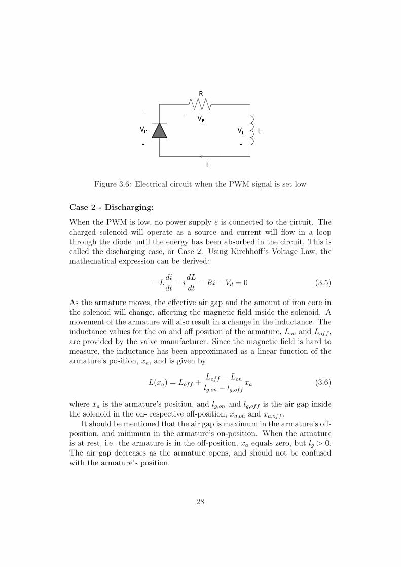
Case 2 - Discharging:

When the PWM is low, no power supply e is connected to the circuit. Thecharged solenoid will operate as a source and current will flow in a loopthrough the diode until the energy has been absorbed in the circuit. This iscalled the discharging case, or Case 2. Using Kirchhoff’s Voltage Law, themathematical expression can be derived:

−Ldi

dt− i

dL

dt−Ri− Vd = 0 (3.5)

As the armature moves, the effective air gap and the amount of iron core inthe solenoid will change, affecting the magnetic field inside the solenoid. Amovement of the armature will also result in a change in the inductance. Theinductance values for the on and off position of the armature, Lon and Loff ,are provided by the valve manufacturer. Since the magnetic field is hard tomeasure, the inductance has been approximated as a linear function of thearmature’s position, xa, and is given by

L(xa) = Loff +Loff − Lon

lg,on − lg,off

xa (3.6)

where xa is the armature’s position, and lg,on and lg,off is the air gap insidethe solenoid in the on- respective off-position, xa,on and xa,off .

It should be mentioned that the air gap is maximum in the armature’s off-position, and minimum in the armature’s on-position. When the armatureis at rest, i.e. the armature is in the off-position, xa equals zero, but lg > 0.The air gap decreases as the armature opens, and should not be confusedwith the armature’s position.

28

3.3.2 Magnetic Model

Due to the current in the coil, a magnetic field will appear inside the solenoidand result in a magnetic force affecting the armature. According to [5], thechange in the magnetic force can be expressed as

dFM

dt=

B2

2µ0

dAp

dt(3.7)

where B is the magnetic field, µ0 is the permeability in air, and Ap = constantis the cross sectional area of the armature.

To make the model as easy as possible, the solenoid has been approximatedto be very long. Then, inside a long solenoid, the magnetic field is givenby [7] as

B = µ0Ni

lg(3.8)

where N is number of turns in the coil, and lg is the air gap inside thesolenoid. The valves are constructed such that the air gap is never zero.This would then result in an infinite large magnetic field. Different air gapsfor the on and off position of the armature have been provided by the valvemanufacturer and can give information on how much the armature moves intotal. As a function of the armature’s position, the air gap is expressed as

lg (xa) = lg,off − xa (3.9)

Combining (3.7), (3.8), and (3.9), the magnetic force can eventually be ex-pressed as

FM =µ0ApN

2i2

2(lg,off − xa)2(3.10)

3.3.3 Mechanical Model

As discussed in the previous section, the magnetic force affects the armature.However, other forces also have an influence on the armature. RecallingSection 2.3, a principle sketch of the valve is shown in Figure 2.1. As seen,the armature is connected to a spring that counteracts the magnetic force.The spring has the spring constant ks and is preloaded with a force Fpld,both provided by the manufacturer. Due to the armature’s connection tothe valve house, static and viscous friction, Fsf and Fb respectively, could bepresent. If pressure supply is connected to the valves, a resulting pressureforce Fprs will also have an influence. In the modelling, Fprs have been

29

assumed to be acting in the positive direction rather than counteracting thearmature’s motion. Newton’s Second Law yields, and together with assumedand provided information, the mechanical model for the valve can be derivedas

mxa = FM + Fprs − Fpld − Fk − Fsf − Fb (3.11)

Pressure force

According to [7] a force due to hydrostatic pressure is given by

F = pA (3.12)

where p is the pressure and A is the affected body area.

As long as the pressure on the inlet port of the valve is bigger than thepressure on the outlet port of the valve, a pressure force will help lifting thearmature in the valve. The resulting pressure force Fprs for each valve, canbe modeled as the difference between the upside (inlet port) pressure and thedownside (outlet port) pressure of the valve, which in mathematical terms isexpressed as

Fprs = Fu − Fd = π(d

2)2(Pu − Pd) (3.13)

where d is the diameter of the affected body area, Fu is the force affectingthe upside, Fd is the force affecting the downside, Pu is the pressure on theupside, and Pd is the pressure on the downside.

Viscous friction

The viscous friction can be modeled according to [7] as

Fb = bv = bxa (3.14)

where v is the armature’s velocity and b is the viscous friction coefficient.

Spring force

The spring force is given by [7] as

Fk = ksxa (3.15)

where xa is the armature’s position.

30

Preload force

The spring is preloaded a certain length, lpld, which is provided by the valvemanufacturer, and corresponds to a preload force, Fpld. The preload force isgiven by

Fpld = kslpld (3.16)

3.3.4 Pneumatic Model

A net force resulting in opening the fill valve leads to an air flow into thechamber and regulating valve. Opposite, ventilation of the dead volume, i.e.an air flow out of the dead volume, will occur if a net force results in liftingthe ventilation valve. If both valves are activated at the same time, therewill be a pressure increase or decrease depending on the net air flow in thedead volume.

The pneumatic model is used to describe the air and heat transfer, andthe expansion and compression relations. Air is a compressible fluid whichbehavior differs from that of a perfect gas. As a pressure supply of Psup isused, which is considered as low pressure (p ≤ 1.0MPa), the deviations froman ideal gas could be neglected. This is not necessarily true since the Re-tarder can be subjected to extreme temperatures, where temperature has aninfluence on the dynamics. However, a controller based on pressure feedbackcan hopefully quickly compensate for errors due to temperature influence,and the temperature variations have therefore not been considered in theearly work. The heat due to compression or expansion is minimal and hasalso been neglected. This is due to an almost constant dead volume and willbe explained further in the next section.

Using the common law of gas [8], the pressure in the dead volume can beexpressed as

Pch =mchRgasTair

Vch

(3.17)

where Pch is the pressure [Bar], Vch is the total dead volume [m3/kg], Rgas isthe gas constant [J/(kgK)], Tair is the temperature in the dead volume [K]and mch is the mass of the air [kg].

The pressure change in the dead volume can now be derived by differen-

31

tiating left and right side of (3.17), and gives

˙Pch =RgasTair

Vch

mch +mchRgas

Vch

Tair

︸︷︷︸≈0

− mchRgasTair

V 2ch

Vch

︸︷︷︸≈0

(3.18)

where it can be seen that the heat and the volume change have been ne-glected.

According to [8], the mass flow for valves, pipes, couplings, filters, etc. canbe calculated according to

mch =CdPuA0√RgasTair

Ψ(Pd

Pu

)ζ (k) (3.19)

where

ζ (k) =

√2k

k + 1

k+1k−1

Ψ(Pd

Pu

) =

1 if Pd

Pu≤ Pcr√

(PdPu

)2k−(

PdPu

)k+1

k

k−12

( 2k+1

)k+1k−1

if Pcr < Pd

Pu≤ 1

where Ao is smallest outlet area, Cd the so called discharge coefficient, andk ≈ 1.4 is the specific heat ratio in air.

The outlet area depends on the armature’s position. If the armature is closed,no air will flow through the valve. As soon as the armature opens, the outletarea gets bigger. The smallest outlet orifice area can be expressed as

Ao = πd0xa (3.20)

where d0 is the diameter of the inlet orifice, and is illustrated in Figure 3.7.

Remember that the outlet area cannot be bigger than the area of the inletorifice. If this is the case, the outlet area has to be saturated to be

Ao = π

(d0

2

)2

(3.21)

which is the cross-sectional area of the inlet orifice.

32

ArmatureA0Air OutAir in

Figure 3.7: The outlet orifice A0

Pcr specifies the critical pressure ratio for a component, e.g. a valve, anddepends on the shape of the orifice in the component. If the ratio betweenthe upside and downside, also called the pressure ratio, is less than the criti-cal pressure ratio, the flow is called a critical flow. For pressure ratios higherthan the critical pressure ratio, the flow is called an under-critical flow. Fora sharp edged orifice the value of Pcr is given by the equation [8]

Pcr = (2

k + 1)

kk−1 ≈ 0.528 (3.22)

The orifice in real pneumatic components often have a different shape and itis not unusual that there are series of orifices that reduce the critical pressureratio. Therefore the Pcr-value is always less than 0.528 for real pneumaticcomponents.

The net airflow to the chamber can be seen as the change in the air mass inthe dead volume, and can be expressed as the mass flow into minus the massflow out of the dead volume.

m = mfill − mvent (3.23)

Inserting (3.23) into (3.18) the pressure change is given by

Pch =RgasTair

Vch

(mfill − mvent) (3.24)

3.4 Regulating Valve

The regulating valve consists of an inlet port, an outlet port, and a plungeconnected to a spring, and is shown in Figure 3.8.Air from the dead volume flows through the inlet port, affecting the plunge.

33

oil

air

Figure 3.8: The regulation valve at its maximum stroke

The plunge moves according to the air pressure in the dead volume and theoil pressure in the retarder, which is connected to the outlet port. Presentin the valve are friction forces and spring forces that counteract the plunge.Figure 3.8 shows the regulation valve at its maximum stroke, where the pos-itive direction is defined as a movement of the plunge from air side to theoil side. The maximum expansion when regulating has been calculated tobe sufficient small compared to the total dead volume of ∼ 100 cm3. Thevolume expansion due to plunge movement in the regulating valve has there-fore been neglected, and the dead volume has been considered constant. If amuch smaller dead volume is used, the expansion could have effects on thesystem’s dynamics and should be considered to be included in the model.

The regulating valve can be modeled using Newtons Second Law, wherethe sum of all the forces working on the system equals zero.

mplungexplunge = Fprs,ch − Fprs,oil − Fk − Ffriction − Fpld

= PchAair − PoilAoil − ksxplunge − Ffriction − Fpld(3.25)

where

Ffriction =

Fsf if xplunge = 0Fdf if xplunge 6= 0

Aair is the affected plunge area on the air side of the valve, and Aoil is theaffected plunge area on the oil side of the valve. From these equations theplunge’s position can be derived. Note that the friction includes two cases,static friction, Fsf , which is present when the plunge is at rest, and dynamicfriction, Fdf , when the plunge moves.

34

3.5 Model Summary

In this section the equations for the complete model have been summarizedin state-space form. First the input signals, output signals and the states aredefined, which is followed by the expressions for all the states.

Input signals:

u1 = uPWM,sup

u2 = uPWM,vent

Output signal:

y = Pch

States:x1 = isupply x2 = xp,sup x3 = xp,sup

x4 = Pch

x5 = ivent x6 = xp,vent x7 = xp,vent

35

State-Space Equations:

x1 =u1 −Rx1

Loff +Loff−Lon

lg,on−lg,offx2

(3.26)

x2 = x3 (3.27)

x3 =µ0ApN

2x21

2mp (lg,off − x2)2 +

π

mp

(d0

2

)2

(Psup − x4)− ks

mp

x2 − b

mp

x3 − Fpld

mp

(3.28)

x4 =

√RgasTaird0π

Vch

(Cd,fillPsupx2Ψ

(x4

Psup

)− Cd,ventx4x6Ψ

(Patm

x4

))

(3.29)

where

Ψ

(x4

Psup

)=

√k

(2

k+1

) k+1k−1 if x4

Psup≤ 0.528√

2kk−1

((x4

Psup

) 2k −

(x4

Psup

) k+1k

)if x4

Psup> 0.528

Ψ

(Patm

x4

)=

√k

(2

k+1

) k+1k−1 if Patm

x4≤ 0.528√

2kk−1

((Patm

x4

) 2k −

(Patm

x4

) k+1k

)if Patm

x4> 0.528

x5 =u2 −Rx5

Loff +Loff−Lon

lg,on−lg,offx6

(3.30)

x6 = x7 (3.31)

x7 =µ0ApN

2x25

2mp (xoff − x6)2 +

π

mp

(d0

2

)2

(x4 − Patm)− ks

mp

x6 − b

mp

x7 − Fpld

mp

(3.32)

36

Chapter 4

Model Validation

When the real system has been modeled, the model has to be verified. Thisis done by comparing the model’s behavior with the behavior of the real sys-tem. Since the real system is not yet available, the two prototypes describedin Section 2.4.2 have been used for verification. The prototypes are physicalmodels of the system to be implemented in the future, and will work approx-imately as the real system. They will give a good indication on how wellthe model represents the true system. Experiments have been performed onPrototype 1 and Prototype 2. Data describing the system’s behavior hasbeen acquired and will be presented here.

Some of the questions concerning the system’s dynamics that are examinedcan be summarized in a list:

• How fast can the dead volume be filled to its maximum, Psup, and to0.26Psup?

• How fast can the dead volume be ventilated from maximum pressure,Psup, to atmospheric pressure, and from 0.88Psup to 0.71Psup?

• Does the flow behave different for pressures close to Psup than for pres-sures close to atmospheric pressure, Patm?

• Are there any time delays in the system?

• For which duty cycles does the armature start to move/oscillate?

• For which duty cycles does the armature stay open?

• Is friction present?

• Does the ventilation valve differ from the filling valve?

37

• How does the frequency affect the valves behavior?

• Does the temperature in the system’s environment have any effects onits behavior?

The PWM-signal used to run the valves consists of a certain frequency fPWM ,and a power supply, e. The chapter is mainly concentrated on two main sec-tions; experiments on Prototype 1 and experiments on Prototype 2. For eachprototype, the system’s characteristics and how it behaves are first examined.This is rather an investigation of different valve and flow properties than avalidation. Eventually a validation of the mathematical model is presented.

4.1 Duty Cycle Limits

It was mentioned in earlier sections that the armature for certain duty cyclescan oscillate between the on and off position. How much it oscillates andhow long determines how much air will pass to the system’s dead volume.An important property to examine, is therefore which duty cycles (DC) arerequired to start moving the valves and to keep the valves fully open. It willalso be seen in the control section that there are certain advantages usingthese duty cycles for closing and opening the valves instead of using mini-mum and maximum possible duty cycles, 0 % respective 100 %.

From experiments, it has been observed that lower duty cycles are needed tomove the armature if the pressure on the valves’ inlet port are higher thanthe pressure on the outlet port. This simply shows that the pressure helpsthe armature to move rather than preventing it from opening, for both thefilling valve and the ventilation valve.

If the pressure on the inlet port is higher than on the outlet port, a move-ment in the armature can be detected if a change in the chamber pressureis detected. It has been observed that the duty cycle where this occurs isdifferent for the fill valve and the ventilation valve, and is probably due tovariations in the friction and preload parameters. Different duty cycles wereapplied to the valves, while the pressure was measured. When the inlet portof the valves is exposed to a pressure of Psup, the results can be summarizedin Table 4.1.

DCmin is the lowest allowed duty cycle to start moving the armature, whileDCmax is the minimum duty cycle that is needed to keep the valve fullyopen. From Table 4.1 it can be seen that the valves open for different duty

38

Fill ValveDCmin,fill 28.5 %DCmax,fill 82 %

Ventilation ValveDCmin,vent 25.5 %DCmax,vent 80 %

Table 4.1: Duty cycle limits for valves to start to open and for valves to keepfully open when a pressure force equal the system pressure helps to open thevalves

cycles. When DCmin is applied to either of the valves, a pressure changewill be detected. Duty cycles lower than DCmin does not generate a currentbig enough to overcome the counteracting forces. For higher duty cycles, thearmature moves with a stronger oscillation and finally keeps open when theduty cycle reach DCmax. However, using a PWM-signal with a duty cycleDCmax, the valves start to oscillate again after a certain period of time. Thisis a phenomena probably coming from a reduced current in the coil due to achange in the coils resistance, and will be handled in upcoming sections.

When the pressure in the dead volume is the same as the system pressure,the system pressure no longer helps the armature in the filling valve to stayopen. The same thing is the case for the ventilation valve when the pressurein the dead volume is atmospheric pressure, i.e. Pup−Pdown = 0 and therebyFprs,vent = 0. In this case the only force acting in the positive x-direction isthe magnetic force. The same duty cycle, DCmax, is therefore needed to keepthe valves fully open whether the armature is exposed to a pressure of Psup

or Patm. The identification of these upper limits is based on the acoustics,i.e. that a motion can be detected if an oscillating sound is heard. Thelimits are for this reason not exact, but with pressure and current as theonly measurable output signals this is the only solution to find the limits.The duty cycle limits when no pressure force helps to open the valves areshown in Table 4.2

4.2 Prototype 1

As described in Section 2.4.2, this prototype consists of a fixed dead volumeof 100 cm3 and valves with an orifice of 1.9 mm. It cannot be mounted onthe truck, and is only used for early testing. In this section important systemproperties for Prototype 1 are examined. A verification of the model is also

39

Fill ValveDCmin,fill 54.5 %DCmax,fill 82 %

Ventilation ValveDCmin,vent 51.5 %DCmax,vent 80 %

Table 4.2: Duty cycle limits for valves to start to open and for valves to keepfully open when no pressure force is acting on the valves

included in this section.

4.2.1 Filling Characteristics

Recalling Section 1.4, the requirements on the filling time is that a pressureof 0.26Psup has to be obtained in less than 0.1Treq. As seen in Figure 4.1(left), it takes approximately Tf = 0.1Treq to obtain 0.26Psup in the deadvolume using 100 % DC, and fulfills therefore exactly the requirements. Asmentioned in Section 2.4.1, the ECU operates at a certain frequency, fECU ,causing a worst case time delay of TECU . It also takes some time for thevalve to overcome counteracting forces, which is the time for the valve toreact. A total time delay, Td, i.e. the time from the control signal is sent,to the valve starts to open, is observed. The delay can vary and depends onthe duty cycles used, and has to be considered in the modeling. Taking thisdelay into consideration, the time to reach 0.26Psup is no longer 0.1Treq, but0.14Treq, and is not satisfying enough.

The time to build up a pressure of Psup in the dead volume takes longer time.The pressure in the dead volume for a duty cycle of 100 % can be seen inFigure 4.1 (right), and shows that a pressure of Psup cannot be reached withinTreq seconds, which was stated as a requirement in Section 1.4. Actually ittakes about 1.4Treq to obtain a dead volume pressure the same as the systempressure, including the time delay.

4.2.2 Ventilation Characteristics

Ventilation occurs when the ventilation valve is open and empties the deadvolume. Air flows to the atmosphere and the pressure in the dead volumedecreases. Also for ventilation there are specific requirements and becomesinteresting when a controller is designed. A prerequisite is that the system is

40

420 422 424 426 428 430 4320

0.1

0.2

0.3

Pch

/Psu

p [N

orm

aliz

ed]

Time [sample]

420 422 424 426 428 430 4320

0.2

0.4

0.6

0.8

1

PW

M d

utyc

ycle

[Nor

mal

ized

]

Pch/PsupPWM Duty Cycle

420 430 440 450 460 470 480 4900

0.2

0.4

0.6

0.8

1

Pch

/Psu

p [N

orm

aliz

ed]

Time [sample]

Td = 0.04 Treq Tf = 0.10 Treq

Figure 4.1: Filling the dead volume with a duty cycle of 100 %, i.e. thevalves are fully open and there is a maximum flow through the valves.

fast enough to fulfill what is required, i.e. the volume has to be small enoughand the orifice big enough to empty the volume in a certain amount of time.A pressure drop from Psup to Patm is shown in Figure 4.2 (right).

780 800 820 840 8600

0.2

0.4

0.6

0.8

1

Pch

/Psu

p [N

orm

aliz

ed]

Time [sample]

780 800 820 840 8600

0.2

0.4

0.6

0.8

1

PW

M d

utyc

ycle

[Nor

mal

ized

]


784 785 786 787 788 789 790

0.65

0.7

0.75

0.8

0.85

0.9

Pch

/Psu

p [N

orm

aliz

ed]

Time [sample]

Tv = 0.08Treq

Figure 4.2: Venting the dead volume with a duty cycle of 82 %

One can see from the figure that a time of 1.4Treq is needed to completelyempty the dead volume, given that the fill valve is deactivated. The time toventilate from 0.88Psup to 0.71Psup takes approximately 0.08Treq as seen inFigure 4.2 (left), and does not fulfill the requirement of 0.05Treq.A conclusion is that a valve with 1.9 mm orifice and a volume of 100 cm3

cannot fulfill the requirements of filling and emptying times.

41

4.2.3 Friction

In most systems there is friction due to contact with e.g. walls or ground. Thedynamic friction coefficient bs has been provided by the valve manufacturer.To identify whether static friction is present or not, one can disconnect thepressure supply, let the dead volume have atmospheric pressure, and let theventilation valve be deactivated. Then no pressure force affects the fill valve.It should be sufficient to investigate the fill valve since the valves are of thesame kind. When the armature does not move, there is no spring force ordynamic friction counteracting the valve. The only forces that are presentare a magnetic force due to applied current to the fill valve, preload forceand possible static friction. A duty cycle just beneath the limit identifiedearlier, is used as input. For this duty cycle the armature just about doesnot move, i.e. that the magnetic force has to overcome preload and staticfriction to move. Calculating the magnetic force by reading the current andsubtracting with the preload force the static friction is identified as

Fsf = FM − Fpld (4.1)

Unfortunately, as was experienced in tests, the provided preload did not seemto be reasonable for a usable model, and had to be adjusted which will bediscussed in the next chapter. Therefore the static friction has not beenidentified with an exact result, but rather been tuned in a reasonable way toget the desired model.

4.2.4 Validation

In this section the model outputs and the outputs from prototype experi-ments will be compared to each other. One of the factors that is vital ingetting a good model is the current used as input to the valves. The ECUcontains a lot of electronics that can be very complex, and as seen in themodeling part, the ECU was simplified significantly. The current is one ofthe outputs that can be validated, and will together with the pressure givean indication of the model’s quality. It has also been seen that the systembehaves different for various duty cycles, so a scheme of different DC’s is inthe last part of the validation section used as input to the system where theresponse has been observed and compared to the model.

Current

Recalling Chapter 3, the inductance in the coil changes according to thearmature’s position, and will for this reason affect the current in the coil.

42

The armature’s position affects the inductance in the solenoid, and therebythe current. Since the armature starts to move for different PWM’s whetherpressure supply is connected or not, the current with pressure supply willdiffer from the current without pressure supply for the same duty cycles.The current in the coil when no pressure supply is connected and a dutycycle of 75 % is applied to one of the valves can be seen in Figure 4.3.

4.74 4.76 4.78 4.8 4.82 4.840

50

100

150

200

250

time [s]

duty

cyc

le [%

] and

cur

rent

[mA

]

Duty Cycle [%]Measured Current [mA]Modeled Current [mA]

Figure 4.3: Current in the coil using a duty cycle of 75 %

From Section 3.3, it was depicted that the current in a solenoid valve chargesand discharges according to (3.2) and (3.5). These equations can be simplifiedby neglecting the freewheeling diode. The voltage balance in the circuit isthen expressed as

UPWM −Ri− Ldidt− i

dL

dt︸︷︷︸≈0

= 0

It is important to know that the freewheel diode has been used in the sim-ulations, and that this simplification just has been done in the manner toportray the solenoid’s nature and time constant. The last term, which is theelectro motive force, is zero when the armature is at rest. This is the casewhen the coil is fully charged, i.e. for infinite charging time, or when thevalves are deactivated. Solving the differential equation, the current can nowbe expressed as

i (t) =UPWM

R

(1− e−

RL

t)

(4.2)

where LR

= τ is the time constant. If a step is applied to the solenoid, whentime elapses to infinity, the solenoid will be fully energized and the current

43

reaches the steady state

limt→∞

i (t) ≈ 292 mA

The current of 292 mA is the maximum current that ever will be present inthe solenoid as long as the parameters provided from manufacturers are used,and corresponds to the maximum magnetic force that can lift the armature.Depending on the duty cycle used for the PWM-signal, the steady currentvaries between zero and 292 mA.

5.76 5.78 5.8 5.82 5.84 5.860

20

40

60

80

100

120

140

160

180

200

time [s]

duty

cyc

le [%

] and

cur

rent

[mA

]

Duty Cycle [%]Measured Current [mA]Modeled Current [mA]

Figure 4.4: Current in the coil using a duty cycle of 40 %

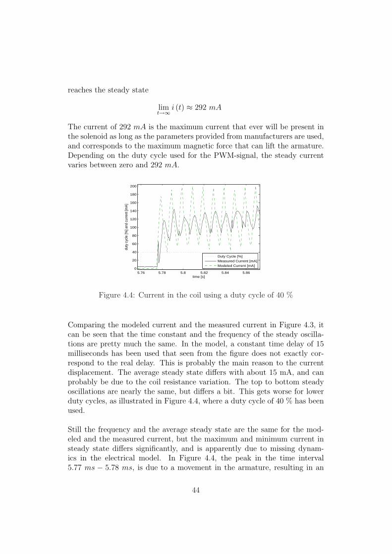
Comparing the modeled current and the measured current in Figure 4.3, itcan be seen that the time constant and the frequency of the steady oscilla-tions are pretty much the same. In the model, a constant time delay of 15milliseconds has been used that seen from the figure does not exactly cor-respond to the real delay. This is probably the main reason to the currentdisplacement. The average steady state differs with about 15 mA, and canprobably be due to the coil resistance variation. The top to bottom steadyoscillations are nearly the same, but differs a bit. This gets worse for lowerduty cycles, as illustrated in Figure 4.4, where a duty cycle of 40 % has beenused.

Still the frequency and the average steady state are the same for the mod-eled and the measured current, but the maximum and minimum current insteady state differs significantly, and is apparently due to missing dynam-ics in the electrical model. In Figure 4.4, the peak in the time interval5.77 ms − 5.78 ms, is due to a movement in the armature, resulting in an

44

induced electro motoric force (emf). When the iron armature moves into thesolenoid, the induced emf counteracts the current already present in the coil,and results in a longer charging time and a slower pressure increase in thedead volume.

Pressure

The pressure in the dead volume determines the braking torque in the re-tarder and is for this reason of high interest to investigate. Both filling andemptying the volume should be studied, using different duty cycles to thevalves. First the filling and venting are studied separately with a duty cyclethat keeps the valves fully open. This will give the fastest filling and ventingtime that is possible in the system and can give an indication of how wellthe pneumatic model coincides with the real flow characteristic. Figure 4.5shows the modeled pressure and the measured pressure when an 82 % dutycycle has been applied to the fill and empty valve separately.

410 420 430 440 450 460 470 4800

0.2

0.4

0.6

0.8

1

Time [Sample]

Pch

/Psu

p [N

orm

aliz

ed]

Measured PressureModeled Pressure

1260 1270 1280 1290 1300 1310 13200

0.2

0.4

0.6

0.8

1

Time [Sample]

Pch

/Psu

p [N

orm

aliz

ed]


Figure 4.5: The modeled pressure and the measured pressure when 82 % dutycycle has been applied to the fill (top) and empty (bottom) valve separately

It can be seen that for this duty cycle the modeled pressure follows verymuch the measured pressure, and is a result of tuning pneumatic parameterssuch as discharge coefficients and critical pressure ratio. The model fills thedead volume a bit faster than what happens in reality. When the pressurein the chamber is close to the system pressure, the air flows slower throughthe valve and is due to different flow patterns, such as choked and unchokedflow, as seen in the pneumatic model in Chapter 3. In the real system,

45

a leak can also be observed, which has not been considered in the model.Figure 4.6 shows the pressure in the dead volume when both valves areactivated simultaneously, using a DC of 82 %. Also for these inputs, themodel corresponds well to the real system. This experiment can be used togive an indication of stationary points suitable for linearization if a modelbased controller is to be designed.

1000 1010 1020 1030 1040 1050 1060 1070 1080 10900.65

0.7

0.75

0.8

0.85

0.9

0.95

1

Time [Sample]

Pch

/Psu

p [N

orm

aliz

ed]


Figure 4.6: Pressure in the dead volume when filling valve and venting valveare both applied a duty cycle of 82 %

As shown in Figure 4.7 the model pressure for low duty cycles does notcorrespond as well to the real pressure as for high duty cycles. The error isat its maximum 50 % and is not satisfying enough. This is believed to be dueto a bad model of the current in the solenoid, which affect the armature, andcan be explained as follows. For lower duty cycles it was seen in Section 4.2.4that the model current was oscillating much more than the real current. Inthe case where the duty cycle was 40 %, the minimum current was around60 mA, and is not enough to lift the armature. The same happens with aduty cycle of 50 %, so the armature is in the model closed for a longer timethan in the real process and can thereby not fill as fast as the valve does inreality as shown in Figure 4.7. As will be seen in the next sections, this willcause problems when operating with lower duty cycles.

Pressure with a scheme of random duty cycles as input

To test for several input signals to the system, a scheme of random dutycycles were generated and used as input to the fill and ventilation valve. Theresult is shown in Figure 4.8Also here it can be seen that the model is far from reality for certain combina-tions of input signals. As already mentioned, a bad current model will affectthe rest of the dynamics dramatically. Because of wrong current amplitudein the model, the armature will switch between the on and off position more

46

300 400 500 600 700 800 900 1000 1100 12000

0.2

0.4

0.6

0.8

1

1.2

Time [Sample]

Pch

/Psu

p [N

orm

aliz

ed]

Pressure Validation

300 400 500 600 700 800 900 1000 1100 1200−20

0

20

40

60

Time [Sample]

Err

or [%

]

Error


Error

Figure 4.7: Pressure in the dead volume when filling valve and venting valveare both applied a duty cycle of 50 %

than in reality for low duty cycles, causing a longer fill or vent time. Since thearmature’s position is not possible to measure, it is very difficult to have anexact understanding of how the armature moves. What is known, is that theinductance changes as the armature moves in and out of the solenoid. Thiscan be seen in the measured current data, and may be of help for improvingthe model. Due to the thesis time restrictions, this has not been investigated.

4.3 Prototype 2

Prototype 2, as described in previous sections, is a physical model that canbe mounted directly on the retarder. The air pressure affects the regulatingvalve that determines the oil pressure in the retarder, which corresponds toa braking torque in the truck. According to calculations done by variousvalve manufacturers, Prototype 2 has been derived with a nozzle of 1.0 mmand a fixed volume of 75 cm3 including the volume in the housing and theregulating valve, to compete with the specification requirements. The volumecan easily be extended by adding extra volume to the chamber mounted onthe prototype, as well as orifices with another dimension can be inserted onthe valve’s inlet port. Friction, open and close duty cycle limits, and currentproperties should all be the same as for Prototype 1, this because the samevalves are used, and will not be investigated for Prototype 2. On the other

47

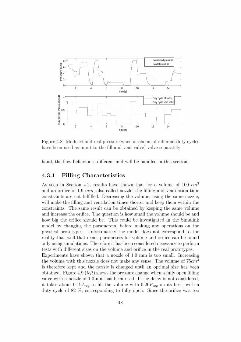
2 4 6 8 10 12 140

2

4

6

8

time [s]

Pre

ssu

re [

Ba

r]

Measured pressureModel pressure

2 4 6 8 10 12 140

0.5

1

time [s]

Du

ty C

ycle

[N

orm

aliz

ed

]

Duty cycle fill valveDuty cycle vent valve

Figure 4.8: Modeled and real pressure when a scheme of different duty cycleshave been used as input to the fill and vent valve) valve separately

hand, the flow behavior is different and will be handled in this section.

4.3.1 Filling Characteristics

As seen in Section 4.2, results have shown that for a volume of 100 cm3

and an orifice of 1.9 mm, also called nozzle, the filling and ventilation timeconstraints are not fulfilled. Decreasing the volume, using the same nozzle,will make the filling and ventilation times shorter and keep them within theconstraints. The same result can be obtained by keeping the same volumeand increase the orifice. The question is how small the volume should be andhow big the orifice should be. This could be investigated in the Simulinkmodel by changing the parameters, before making any operations on thephysical prototypes. Unfortunately the model does not correspond to thereality that well that exact parameters for volume and orifice can be foundonly using simulations. Therefore it has been considered necessary to performtests with different sizes on the volume and orifice in the real prototypes.Experiments have shown that a nozzle of 1.0 mm is too small. Increasingthe volume with this nozzle does not make any sense. The volume of 75cm3

is therefore kept and the nozzle is changed until an optimal size has beenobtained. Figure 4.9 (left) shows the pressure change when a fully open fillingvalve with a nozzle of 1.0 mm has been used. If the delay is not considered,it takes about 0.19Treq to fill the volume with 0.26Psup on its best, with aduty cycle of 82 %, corresponding to fully open. Since the orifice was too

48

364 366 368 370 372 374 376 3780

0.05

0.1

0.15

0.2

0.25

0.3Pc

h/Ps

up [N

orm

alize

d]

Time [sample]

364 366 368 370 372 374 376 3780

0.2

0.4

0.6

0.8

1

1.2

PWM

dut

ycyc

le [N

orm

alize

d]


870 872 874 876 8780.65

0.7

0.75

0.8

0.85

0.9

Pch/

Psup

[Nor

mal

ized]

Time [sample]

Tv = 0.15 Treq


Figure 4.9: Filling (left) and ventilating (right) the dead volume with andorifice of 1.0 mm

small, it was increased to be 1.3 mm. The results can be seen in Figure 4.10.Also for this orifice size, the filling and ventilation are too slow. Changingthe orifice to 1.9 mm, the fastest fill time is of 0.066Treq for a duty cycle of100 %, and is shown in Figure 4.11 (left). If the valve response time and theECU time delay is to be considered, which is 0.04Treq, then the filling timeis 0.106Treq, and is very close to fulfill the time constraints.

480 485 4900

0.05

0.1

0.15

0.2

0.25

0.3

Pch

/Psu

p [N

orm

aliz

ed]

Time [sample]

480 485 4900

0.2

0.4

0.6

0.8

1

PW

M d

utyc

ycle

[Nor

mal

ized

]


382 384 386 388 3900.65

0.7

0.75

0.8

0.85

0.9

Pch

/Psu

p [N

orm

aliz

ed]

Time [sample]


Tv = 0.092 Treq

Figure 4.10: Filling (Left) and ventilating (Right) the dead volume with anorifice of 1.3 mm

4.3.2 Ventilation Characteristics

For the same orifices, the ventilation characteristics have been examined. Thebigger the orifice is, the faster is the ventilation of the dead volume. Theresults are shown in Figure 4.9 (Right), Figure 4.10 (Right), and Figure 4.11

49

(Right). Examining the figures, one can conclude that also for venting thedead volume, the orifices of 1.0 mm and 1.3 mm are too small to empty thedead volume fast enough. The prototype having an orifice of 1.9 mm and avolume of 75 cm3 is the one that closest fulfills the requirement of ventilationof 0.05Treq.

486 488 490 4920

0.05

0.1

0.15

0.2

0.25

Pch

/Psu

p [N

orm

aliz

ed]

Time [sample]

486 488 490 4920

0.2

0.4

0.6

0.8

1

PW

M d

utyc

ycle

[Nor

mal

ized

]


1178 1179 1180 1181 1182 11830.65

0.7

0.75

0.8

0.85

0.9

Pch

/Psu

p [N

orm

aliz

ed]

Time [sample]

Tv = 0.052Treq

Td = 0.04Treq

Tf = 0.066Treq

Figure 4.11: Filling (Left) and ventilating (Right) the dead volume with andorifice of 1.9 mm

Summarizing the results from filling and ventilation experiments for Proto-type 1 and 2 in Table 4.3, one can conclude that a volume of 75 % and anorifice of 1.9 mm is the only available prototype that is close to fulfill thetime constraints on filling and ventilation of the dead volume.

Table 4.3: Filling from Patm to 0.26Psup and ventilation from 0.88Psup to0.71Psup

PrototypeDead

VolumeOrifice

DiameterFilling

Patm to 0.26Psup

Venting0.88Psup to 0.71Psup

P1 100 cm3 1.9 mm (0.04 + 0.10)Treq 0.08Treq

P2 75 cm3 1.0 mm (0.02 + 0.19)Treq 0.15Treq

P2 75 cm3 1.3 mm (0.06 + 0.132)Treq 0.092Treq

P2 75 cm3 1.9 mm (0.04 + 0.066)Treq 0.052Treq

The results can be used to give an indication on how big the volume andthe orifice should be. To fulfill the requirements, the dead volume should bea bit less than 75 cm3 and an orifice of 1.9 mm, or the orifice a bit bigger

50

Table 4.4: Filling from Patm to Psup and ventilation from Psup to Patm

PrototypeDead

VolumeOrifice

DiameterFilling

Patm to Psup

VentingPsup to Patm bar

P1 100 cm3 1.9 mm (0.04 + 1)Treq 1.4Treq

P2 75 cm3 1.0 mm (0.02 + 1.2)Treq 2.4Treq

P2 75 cm3 1.3 mm (0.06 + 1.1)Treq 1.6Treq

P2 75 cm3 1.9 mm (0.04 + 0.74)Treq 1.16Treq

with a volume of 75 cm3. Having a bigger orifice than 1.9 mm would implythat a bigger valve should be needed, which could result in a slower valveresponse and more time delays in the system. A smaller volume is thereforeto be preferred.

4.3.3 Validation

It should be sufficient to verify the model for one orifice since this is the onlyparameter that differs through the experiments on Prototype 2. The orificeof 1.0 mm has been chosen in the verification. In order to validate the modeland the prototype, the model has to be modified by changing the orifice andthe volume. Since the orifice has been inserted in the valve housing, theaffected armature area by the pressure can still be thought to be the areawith diameter 1.9 mm, since this is the fixed orifice in the valve, and can beseen in Figure 4.12.

Orifice 1.0 mm ValveHousing 1.0 mm 1.9 mmFigure 4.12: Inserted orifice of 1.0 mm in the inlet port of Prototype 2

As was done for Prototype 1, the modeled pressure and the measured pressurewill be compared, both for filling and venting the dead volume.

51

Pressure

A duty cycle of 82 % is first applied to both the filling and ventilation valveseparately to fill from Patm to Psup, respective ventilate from Psup to Patm.For this duty cycle, the armature is fully open in both model and reality, sothat the pressure does not depend on the armature’s position. In this waythe pneumatic part can be verified. The simulation and the measured datafor the pressure when 82 % duty cycle was used are shown in Figure 4.13.

360 370 380 390 400 410 420 430 4400

0.2

0.4

0.6

0.8

1

time [s]

Abs

olut

e P

ress

ure

[Bar

]

Filling: Orifice 1.0 mm and Volume 75 cm3


860 880 900 920 940 960 980 1000 10200

0.2

0.4

0.6

0.8

1

Time [Sample]

Pch

/Psu

p [N

orm

aliz

ed]

Venting: Orifice 1.0 mm and Volume 75 cm3


Figure 4.13: Filling and Ventilation Verification with 1.0 mm orifice, 75 cm3

volume, and 82 % applied duty cycle to fill and vent valve separately

Filling and ventilation of the dead volume takes approximately the sametime in the model as in reality, about 1.1Treq respective 2.4Treq. On theother hand, the curves do not correspond that well in the transreal phase.

As was the case for Prototype 1 for low duty cycles, that problem willnot disappear using another prototype. The same will happen here. Theresults for a duty cycle of 60 % is shown in Figure 4.14 and as can be seen,the valves are too weak to fill and vent to the real levels in the same time.With this result it can again be concluded that in reality the valves switchless between the on and off position and are open for a longer time duringthe period the fill or vent valve is activated, which makes the fill- and ventresponse much faster.For duty cycles lower than 60 %, the results are even worse, and can in worstcase deteriorate the performance of a model based controller.

52

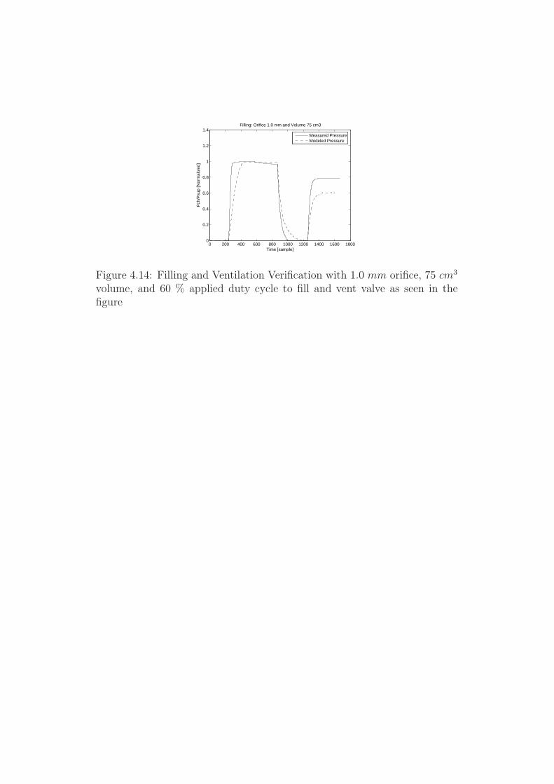
0 200 400 600 800 1000 1200 1400 1600 18000

0.2

0.4

0.6

0.8

1

1.2

1.4

Time [sample]

Pch

/Psu

p [N

orm

aliz

ed]

Filling: Orifice 1.0 mm and Volume 75 cm3


Figure 4.14: Filling and Ventilation Verification with 1.0 mm orifice, 75 cm3

volume, and 60 % applied duty cycle to fill and vent valve as seen in thefigure

Chapter 5

Model Refinements

Modeling a system often requires a knowledge of many physical parametersconcerning the system’s dynamics. This could be parameters describing theairflow through an orifice, the magnetic field in a solenoid, the damping forcesin the valve or time delays in the electronic control unit. A model is only anapproximation of a real system and special cases are very often consideredin the model design. Parameters used are mostly based on normal cases,but in the real world not every system is similar. Therefore it is in manycases necessary to change the model parameters to match the system thatis studied. If real data can be obtained, the model can be compared to thereal data. Parameters can up to a certain level be tuned so that the modeland the system match each other. This is called parameter tuning and willbe part of the content in this chapter. Other factors that can improve themodel will also be handled.

5.1 Parameter Tuning

Factors that have been observed to affect the system significantly are the airgap in the valve, the discharge coefficient Cd, the spring preload force Fpld

and the valve inlet orifice A0.

5.1.1 Air Gap

From the valve manufacturer, data such as coil resistance, inductance, andair gap inside the solenoid has been provided. The air gap is one of thefactors determining the magnetic force which is influencing the armature.Interpreting (3.10), a smaller gap generates a stronger magnetic force, whichis due to a stronger magnetic field in the gap. Using manufacturer provided

55

data, a model was obtained that far from the real data matched the realsystem. In the armature on-position, the provided air gap corresponded toa so strong magnetic force causing the valves to keep fully open already forduty cycles below 60 %, while in fact the limits are 82 % and 80 %.

According to the valve manufacturer it was clear that the air gap insidethe solenoid changed when the armature moved, between lg,on and lg,off ,which is the length of the air gap in the on and off position. However, the totalair gap that results in a magnetic field inside the solenoid does not necessarilychange as much as the provided air gap, which can be explained in a simpleway using Figure 2.1 in Chapter 2 as reference: When the armature startsto move, the air gap between the armature and the inlet port (outside thesolenoid) increases, while the air gap on the back side of the armature (insidethe solenoid) decreases. In the on-position, the inside air gap has reached itsminimum, lon, while the air gap outside the solenoid is maximum. Takinginto consideration the air gap outside the solenoid, the effective air gap canbe considered almost constant. The magnetic field is hard to measure, andthe magnetic field lines are therefore hard to have an understanding of. Usinga nearly constant air gap has therefore been seen as a reasonable solution,and a model more similar to the real system was obtained.

5.1.2 Discharge Coefficient, Cd

John C. Kayser and Robert L. Shambaugh [11] defined the discharge coef-ficient as the ratio of the actual mass flow rate to the isentropic, adiabaticmass flow rate which hypothetically would occur given identical upstreamtemperature, upstream pressure, and pressure drop.

Cd =mactual

misen,adiabat

=

∫ ∫A2

ρ (~v~n) dA

misen,adiabat

(5.1)

where misen,adiabat is the isentropic, adiabatic mass flow rate [kg/s], A is thecross-sectional area of a converging nozzle, A2 is the minimum cross-sectionalarea of a converging nozzle [m2], v is the velocity [m/s], mactual is the actualmass flow rate [kg/s], and ~n is the normal vector.

As seen from (5.1) the discharge coefficient is a convenient scaling of themass flow surface integral, i.e. that it depends on the shape of the ori-fice. J.C.Kayser and R.L.Shambaugh [11] presented in 1991 a study of thecompressible-flow behavior of light gases through small orifices and conver-gent nozzles with diameters ranging from 0.9 to 1.9 mm. Different shapes oforifices were studied; knife-edge, straight-bore, rounded-entry and elliptical-entry orifices. Concluded was that most shapes have a discharge coefficient

56

near unity for Reynolds number between 20000 and 100000. However, othervalues of the discharge coefficients could be real for lower Reynolds numbersor for orifice geometries where the length-to-diameter ratios are greater thanunity. For these cases, the discharge coefficient was identified to be between0.6 and 1. The former results have been used as a reference in finding thedischarge coefficient for the valves used in this Master’s Thesis.

Figure 5.1 shows how the pressure in the dead volume changes when a stepis first applied to the fill valve, then to both valves simultaneously, using dif-ferent discharge coefficients for the fill valve. Here the discharge coefficientfor the ventilation valve is set to a constant value 0.97. One can see that aCd closer to one makes the fill valve fill faster.

0.6 0.8 1 1.2 1.4

2

4

6

8

10

time [s]

pres

sure

[bar

]

Cd,sup=0.60Cd,sup=0.75Cd,sup=0.90

0.5 0.6 0.7 0.8

2

4

6

8

10

time [s]

pres

sure

[bar

]

Cd,sup=0.60Cd,sup=0.75Cd,sup=0.90

Figure 5.1: Pressure Change in the Dead Volume as Different Cd’s are usedfor the Fill Valve when Fill Valve is first activated, then both valves si-multaneously (Left). Zoomed plot of the Filling Characteristics (Right).Cd,vent=0.97.

The discharge coefficient is varied until the measure data and the simulateddata for the pressure corresponds to each other. A discharge coefficient closeto unity as seen in the figure is used to get the same fast response in themodel as have been observed in the true system.

5.1.3 Force Balance

As mentioned earlier, the spring is preloaded a certain length to keep thevalve from opening when the valves are affected by higher pressure than theatmospheric, and to always keep the spring in a stiff mode. Static frictionhas been discussed to be present due to contact with the walls, and would

57

in this case also prevent the valves from opening. When the system modelfirst was derived, data for preload force, valve orifice diameter, spring coef-ficient, air gap, and damping coefficient provided by the manufacturer, wereused in simulations. Experiments have shown that the output in pressureand current for the model does not match the outputs from the real system;the modeled valves start to open and keep open for duty cycles even lowerthan the limits identified in experiments. Either the preload force or thestatic friction have been assumed too weak, or the inlet orifice too big. Inorder to let the modeled valves open for the same DC limits as identified,the parameters have been considered necessary to tune.

Increasing the preload force or the static friction and keeping the other pa-rameters constant makes the valves open closer to the DC limits. Tuning itso that the lower limit is correct makes the upper limit, i.e. the DC wherethe valve keeps open, too high. To still keep the lower limit correct, Fsf orFpld could be decreased while the orifice, corresponding to a pressure force,is adjusted. In this way, correct values for both the lower and the upperlimit can be obtained. The orifice only affects the valve as long as there is apressure difference between the upper and downer side of the valve. In otherwords, changing the orifice will not affect the upper limit, since Pu−Pd = 0,and thereby Fprs = 0, when the valves stay fully open. In order to tune themodel so that the limits are correct, it has been a matter of adjusting thepreload force, the friction and the orifice.

5.1.4 Valve inlet orifice

The valve inlet orifice diameter is the size of the inlet port and is given bythe valve manufacturer as 1.9 mm. The orifice determines how much air canpass through the valve and into the dead volume. The bigger this orifice is,the more air can pass through.

Recalling (3.13), one can see that another effect of having a big orifice isthat less magnetic force has to be applied to the solenoid to open the valve,since the pressure force affects a bigger area helping the armature to open.Seen from experiments is that the fill valve and the ventilation valve startsto open for 28.5 % duty cycle respective 25.5 % duty cycle when they areexposed to a pressure of Psup, presuming that there is atmospheric pressureon the outlet port of the valves. As seen in the previous section, in orderto let the valves keep open at 82 % / 80 % duty cycle, the preload forcewas increased. As depicted earlier, having a correct upper limit causing anerror in the lower limit, so the orifice area was increased. This was done with

58

the motivation that the geometry of the valve is pretty complex and hardto have an opinion of. It is believed and presumed from valve descriptionsand sketches that a bigger area affects the mechanics in the valve, with thesame principle as a bigger orifice affected the mechanics in Prototype 2 withan orifice of 1.0 mm in Section 4.3.3. Remember that the orifice also affectsthe flow in the pneumatic part. Increasing or decreasing the area that affectsthe armature to move in the mechanical part, does not mean that air flowsthrough a smaller or bigger orifice. This area should therefore always be keptconstant so that the flow model is kept correct.

5.2 Time Delay

Results from the model validation in Chapter 4 shows that it takes a certaintime for the valve to respond from the control signal is sent to the valve.It was stated that this was partly due to a valve response time, which isthe time it takes for the coil to energize, but also because of a delay in theECU, due to the limited ECU sampling frequency, fECU . To compensatefor this delay, a time delay block in Simulink has been inserted. An effectof the time delay is that it takes longer time to close or open the valvesthan expected. In the controller design this has to be considered, since thevalves will continue filling or venting as long as no control signal has been”noticed” by the valves. A possible solution could be to deactivate the valvesa bit before we actually want the valves to be deactivated. Experiments haveshown that the time delay depends on the duty cycles used as input signals tothe valves. In Figure 5.2 time delay is illustrated using DC=75 % and DC=40% respectively. In the model, a constant time delay was used to model timedelays, but a model depending on the input signal could be considered infuture work to get a more correct model.

5.3 Temperature Dependent Resistance

It appears from experiments that the current through the conductor decreaseswhen the valves are activated for a longer period of time. This is due tothe fact that the temperature in the valves increases as voltage is applied,resulting in a change in the coil resistivity. According to [9], the resistanceis proportional to the resistivity. In this way, the resistance can directlybe expressed in terms of the temperature. Taking into consideration thetemperature dependent resistance, a more correct model can be obtainedfor the On/Off Retarder system. However, this is not necessarily the best

59

4.74 4.742 4.744 4.746 4.748 4.75 4.752 4.754 4.756 4.7580

50

100

150

200

time [s]

duty

cyc

le [%

] and

cur

rent

[mA

]

Duty Cycle [%]Measured Current [mA]

3.9 3.902 3.904 3.906 3.908 3.91 3.912 3.914 3.916 3.918 3.92

0

20

40

60

80

100

120

time [s]

duty

cyc

le [%

] and

cur

rent

[mA

]

Duty Cycle [%]Measured Current [mA]

Time Delay

Time Delay

Figure 5.2: Current in the coil for DC = 75 % (top) and DC = 40 % (bottom)

solution, since as simple dynamics as possible is desirable when a controlleris to be designed. How the current varies with the time when one of thevalves is activated can be seen from Figure 5.3.The first law of thermodynamics states that the internal energy Eint storedin a thermodynamic system is conserved. According to [9] the change ininternal energy ∆Eint is equal to the energy transfer to the system by heatQ and the work W done on the system.

∆Eint = Q + W (5.2)

The internal energy for an ideal gas is according to [7] given by

∆Eint = nRgas∆T

k−1where k = Cp

Cv≈ 1.4 (5.3)

The temperature in the surroundings, Tsurround, either cools or heats thesystem. A voltage applied to the valves, can be considered as a work doneon the system, and results in further increase of the temperature in the coil.The heat and work is given by

Q = −C(T − Tsurround) (5.4)

W = Ri2 (5.5)

60

10 20 30 40 50 60

270

275

280

285

290

295

time [s]

curr

ent [

mA

]

current [mA]PWM dutycycle [%]

Figure 5.3: Current in the conductor at room teperature, Tsurround = 273 K,when a PWM signal of frequency, fPWM , and 100 % duty cycle have beenused as input.

Combining (5.3), (5.4), and (5.5) an expression for the change in the tem-perature can be derived.

T =k − 1

nRgas

(Ri2 − C(T − Tsurround)) (5.6)

where n is the number of moles, T is the temperature in the coil, C is a heattransfer coefficient, and Tsurround is the temperature in the surroundings.

The resistance in the coil is given by

R = R0(1 + α (T − T0)︸︷︷︸∆T=T

) (5.7)

where T0 is the initial temperature at rest. From these relations, the re-sistance can be modeled. As simple dynamics is desired, the effect of theresistance has been neglected with the motivation that its dynamics is veryslow compared to the total period of time the valves are activated. This canalso be seen in Figure 5.3. The current decreases from about 292 mA to273 mA in 60 seconds, which is slow compared to the time the valves areactivated. It can be concluded that this effect is not only due to a long valveactivation time, but is also present if the truck is used in extreme surroundingtemperatures.

61

5.4 System Identification

As seen from the validation part for the current, the model error is largefor low duty cycles. As stated in Section 4.2 this is due to dynamics in thereal process, more specific in the ECU, which has not been considered in themodel. An alternative is to model all the electrical drives included in theECU, which could be a very complex approach. Using system identificationto model the current could be an alternative approach to the mathematicalequations used for the electrical model for the valves. This can be done usingSystem Identification Toolbox in Matlab. Using the circular flow principlepresented in Figure 5.4, an ARX1 model of the electrical part of the valvesis created. As seen in the figure, the first part of the identification process isto gather data.

Construct experiment and

gather data

Polish and study data

Accommodate model to data

Does data need to be filtered?

Choose model structure

Evaluate model

Can model be accepted?

Data

Data

Model

No

Model structureNot OK

Data Not OK

Yes

Figure 5.4: System identification’s circular flow. The rectangles are the com-puter’s main responsibilities, and the ovals are user’s main responsibilities. [3]

The input and the output are then defined in separate vectors, and as longas filtering is not required a linear model describing the relationship betweenthe input and output is generated. Eventually the model is validated. Forbest results, an altering input signal consisting of both high and low dutycycles, should be used. If this is not done, i.e. the input signal is based on

1ARX model is a type of linear parametic model, which is described by:

A(q)y(t) = B(q)u(t) + e(t) (5.8)

62

one specific duty cycle, the identification may give a poor result. Because ofthe limitations on time for the project, the method has only been tested fora constant input, and due to non-satisfying results system identification hasnot been implemented in the model. However, better results are thought tobe obtained using a wider range of inputs.

63

Chapter 6

Control Design

A natural part of driving is to accelerate and to decelerate. Decelerationrequires a braking torque slowing down the truck’s speed, which depends onhow much the driver wants to slow down. As mentioned in the introduction,the retarder plays an important role in the braking process, and is the onlycomponent in the braking system that is considered in this Master’s Thesis.

One of the main objectives in the thesis is to make a model correspond-ing to the real system, so that a controller based on the model parameterscan be made to control the opening and closing of the valves, determiningthe desired braking torque. The only available output is thought to be thepressure in the dead volume so that a pressure feed back principle can beused. As will be seen, two main approaches are developed and evaluated,denoted Scheme 1 and Scheme 2. Scheme 2 is left to the parallel work [13]performed by Maisam Jeddi Tehrani. This Master’s Thesis will focus onScheme 1, but will briefly introduce Scheme 2 and compare the two methodsin the last part of the control section.

6.1 Background

A common approach in control design is to start with a simple control design.Based on experience from employees at Scania and results from former Mas-ter’s Thesis on On/Off control of exhaust gas recirculation [12], PID controlusing a pressure feedback principle has been used as the base in the controldesign. Additional to the PID controller, intuitive rules, a boosting actionusing non-linear control and prediction is introduced for improvements, andhas been examined closer in upcoming sections. Giving the modeling part ameaning, a model based controller is of interest to examine. Due to model

65

errors and time restriction on the thesis, a real-time tuned PID controllerhas been developed and evaluated instead. The differences between a modelbased and a tuned controller will be discussed in the next section.

6.2 PID Control

Proportional-Integral-Derivative Control, thereby PID control, is widely usedin the industry today and has gained a high popularity due to its simplicityand often good performance for many applications. Previous researchershave used PID control to control solenoid valves for pneumatic actuators [12,15], with successful results. Van Varseveld and Bone [15] implemented andexamined the use of a PID controller combined with four PWM valve pulsingschemes to control the valve position in a electro-pneumatic actuator system,and Hakansson and Johnson [12] developed a PID controller and a Fuzzycontroller for a similar electro-pneumatic actuator system, where the PIDseemed to have as good performance as the Fuzzy controller.

6.2.1 Control Structure

There are mainly two control structures for a PID-controller; error feedbackand output feedback [10]. If Gp is the process we want to control, and Gc isthe controller, the error feedback structure looks like the one in Figure 6.1,where r is the reference, u is the control signal, y is the output signal, and eis the error. GpGc+ - yur e

Figure 6.1: Error Feedback Structure

The output feedback structure is shown in Figure 6.2, and is equipped witha feed forward block, Gff . With the output feedback structure more designfreedom can be achieved, due to the feed forward part that can be usedfor pole cancellation and separate derivative action on the reference signal.In this Master’s Thesis only the error feedback is considered, hence outputfeedback is not described further.

66

Gp+ - yr GcuGff

Figure 6.2: Output Feedback Structure

Error Feedback

A control law for the PID-controller using the error feedback principle isaccording to [10] in continuos time given by

u (t) = Pe (t) + Dde (t)

dt+ I

t∫

t0

e (t) dt

= K

e (t) + Td

de (t)

dt+

1

Ti

t∫

t0

e (t) dt

(6.1)

where K is the gain, Td is the derivative action time constant, and 1Ti

is theintegral action time constant. The error, which is the difference between thereference pressure and the actual pressure, is manipulated by a proportional,derivative and integral action, and used as the new input to the process,which is called the control signal u.

The control signal

The control signal is a PWM signal that shall activate the valves. As aPWM signal runs with a certain duty cycle for a specific frequency, these arethe parameters of interest when creating the control signal. In the controldesign, the case when a fixed frequency, fPWM , and a varying duty cycle hasbeen used, has been investigated. According to the valve manufacturer, thefrequency could also be varied to get an improved control performance. Apossible solution is then to keep the off-time of the valves and the duty cycleconstant, so that when the frequency is changed, the on time varies, andcorresponds to different mass flow through the valves. The approach wouldbe very interesting to further investigate, but the lack of time did not allowit.

67

Proportional action

When there still is an error between the reference and the actual output value,the error should as fast as possible be compensated for so that the referencecan be reached. The proportional part, also called the gain, K, is used toamplify the error to get a faster action on the control signal. Choosing a toohigh gain can result in oscillations in the output, or even instability in thesystem.

Derivative action

The derivative part differentiate the error and uses the result as a subsidy inthe control signal to compensate for error in the output signal. Its intentionis to decrease the oscillations on the output caused by a high gain. Thederivative action is highest when the change in the error is high, and is leastsignificant when the change in the error is low.

Integral action

The integral part has as intention to remove stationary error on the output.When the error is positive, the control signal increases due to integral action,and when the error is negative, the control signal decreases. The integralaction is slower than the derivative and proportional action.

6.2.2 Model Based Control

A model based controller calculates a set of control parameters, K, Td andTi based on a linear model of the system. There are several approaches tothis. Among the alternatives is a method solving the Diophantine equation,which is used thoroughly through examples in the course literature [10]. Themodel based approach requires that the system is linear. The system in thisMaster’s Thesis is non-linear, so the model has to be linearized in order touse this approach. The linearized model can be found in the appendix, butbecause of lack of time, there has not been invested more time in developinga model based controller.

6.2.3 Tuned Controller

A very common approach in the industry today, is to directly apply a tunablecontroller to a system, i.e. that a controller with adjustable parameters canbe applied to a system without any knowledge about the system. The samekind of controller will be developed and used in this work. In many cases, this

68

approach cannot be used because of security reasons or because the systemdoes not exist.

An indication on how the parameters should be chosen can be obtainedthrough simulations where the parameters can be adjusted. A reference signalis generated and applied to the discrete hard-ware implemented controller.With a real-time software, data such as the reference, the output and thecontrol signal can be acquired in real-time. Adjusting the control parameterswhile comparing the real time data, a desired set of parameters have beenfound when the desired control behavior is achieved. Both Ziegler-Nicholsmethod and Astroms rules have been used as reference for the choice ofPID-parameters [17].

6.2.4 Implementation

For simulations in computer programs such as Simulink, a continuos timecontroller is sufficient. This is not true if the controller is to be implementedin a real system, which mostly is the case. Then a discrete time controllerhas to be implemented and is given by

un = K

(en + Td

en − en−1

Ts

+Ts

Ti

n∑

k=0

ek

)(6.2)

where Ts is the sample time and en is the sampled error at sample n.

6.3 Approaches

The PID-controller generates a control signal based on the error. A positiveerror means that the pressure in the dead volume is too low compared to thereference pressure. Opposite, if the error is negative, the pressure is too high.Basically, seen from (6.1), the generated control signal is positive for positiveerror and negative for negative error. Since there are two valves and just onecontrol signal, the controller has to distribute the signal to the two valves.A controller including a distributor can look like the setup in Figure 6.3.There are several ways for the distributor to handle how the valves shouldwork for different control signals, e.g. if both valves should act simultaneouslyor separately, if the whole control signal range should be used or not etc.Based on earlier research mentioned in the introduction, two different waysof doing this have been investigated, where one of the approaches will beinvestigated in this Master’s Thesis and the other is left for the parallelwork [13].

69

y

y

1

Plant

Gp

Distributor

u

ufill

uvent

fcn

Controller

error u

r

1

Figure 6.3: A setup with the controller and a distributor distributing thecontrol signal to either of the two valves

6.3.1 Scheme 1 - Fill valve and Empty valve activatedseparately for filling and venting

The distributor uses a PWM pulsing scheme where the control signal is re-solved into two individual pulsing of the two valves, fill and ventilation valve.If the control signal is positive the fill valve is activated, and if negative, theventilation valve is activated. Pulsing Scheme 1 is based on a traditionallinear approach as seen in Figure 6.4 (left) where the control signal is lin-early resolved into the two pulsing. Notice that the valves can only react forpositive duty cycle values, therefore the absolute value of the signal is sentto the valves. This can be summarized in the following equations.

ufill = uuvent = 0

for u > 0 (6.3)

ufill = 0uvent = |u|

for u < 0 (6.4)

ufill = 0uvent = 0

for u = 0 (6.5)

One of the drawbacks with this approach is that for control signals in theinterval [−DCmin,vent, DCmin,fill], the valves will not react, meaning that thecontrol signal contains a dead band. From the validation in Chapter 4 itwas seen that a duty cycle of DCmax was sufficient to fully open the valves.Using a higher duty cycle as in the traditional linear approach, the valveswill be over magnetized, causing the coil to discharge even slower, resultingin a longer time to close the valves when needed. To prevent these two phe-nomenas, Pulsing Scheme 1 has been developed, where the output from thedistributor can be seen in Figure 6.4 (right).Now the duty cycle range [0, 100] is resolved and linearized into the activerange [DCmin, DCmax] instead, so that the dead band is nearly eliminated.

70

−100 −50 0 50 100

0

20

40

60

80

100

Control Signal − u [%]

Val

ve D

uty

Cyc

el [%

]

PWM Pulsing Scheme 1

−100 −50 0 50 100

0

20

40

60

80

100

Control Signal − u [%]

Val

ve D

uty

Cyc

el [%

]

Traditional Linear Scheme

Empty ValveFill Valve

Empty ValveFill Valve

Figure 6.4: Traditional Pulsing Scheme (left) and Pulsing Scheme 1 (right)

The reason why this only holds almost, is connected to the fact that Puls-ing Scheme 1 does have a drawback letting both valves be DCmin when thecontrol signal is zero. Setting one of the valves to DCmin when the valveis desired to be deactivated would give a faster response when the valve isto be activated again. What is not so good is that when the valve shoulddeactivate, it would take much longer time to discharge the coil, and therebyclosing the valve. This will result in a delay that may give a poor controlperformance. Therefore Pulsing Scheme 1 has been extended by includingan error tolerance. When the error is within the predetermined tolerance,both valves should be deactivated. The tolerance has been chosen to be therequired control tolerance on ± Ptol as required in the specifications.

Letting the valves operate separately, i.e. using Scheme 1, a minimum use ofthe valves could be possible, since one of the valves is always at rest. This isan advantage considering the life time of the valves.

6.3.2 Scheme 2 - Both valves activated simultaneouslyfor filling and venting

The pulsing scheme is based on results from former research [15] where a socalled novel pulsing scheme was designed to remove non-linear response in theoutput. The method is based on a distributor that resolves the control signalinto the two valves, with a possibility to activate both valves simultaneously.In this way there is more freedom in combining the two valves to get thedesired air pressure.

71

6.4 Results - Scheme 1

The controller is first implemented and simulated in Simulink. Doing this,the regulator is tuned until a desired set of control parameters have beenobtained. The parameters identified from the simulations are then used asreference when tuning the controller in the real system.

6.4.1 Simulations

Using a valve orifice of 1.3 mm and a volume of 75 cm3, the simulation resultsof a PID-controller can be seen in Figure 6.5.

2 4 6 8 10 12 14 160

2

4

6

Time [s]

Rel

ativ

e P

ress

ure

[bar

]

Pressure in Dead Volume

PchPref

2 4 6 8 10 12 14 160

20

40

60

80

100

Time [s]

Dut

y C

ycle

[%]

Control Signal

DC fillDC vent

Figure 6.5: Resulting PID-controller in simulations, using an orifice of1.3 mm and a volume of 75cm3

The control signal is better seen in Figure 6.6 where the controller’s behaviorclearly shows that close to the reference, the control signal decreases, meaningthat less action is needed. The reason that the output never exactly reachthe reference for any reference pressures is that the tolerance of ± Ptol hasbeen applied to the controller, i.e. when the error is less than this tolerance,the valves will be deactivated. This has been done with respect to the realsystem, where oscillations would be a result of not having the tolerance. Itis thereby not said that oscillations cannot arise, but the tolerance is ratherused to decrease eventual oscillations. Looking at Figure 6.5 again, one cansee from the control signal that only one valve acts at the moment, whichis the idea with scheme one. An example showing the integral part acting,can be drawn by looking at the time period from t ≈ 4 s to t ≈ 5 s. The

72

fill valve is first activated, but has a too strong effect such that the pressurerises over the reference and even outside the tolerance. The controller hasto ventilate the dead volume until the error is within the tolerance. Thecontrol signal is in this area seen to be integrating until the valve reacts andempty the dead volume. When the desired pressure is reached, the valve isdeactivated. The controller works fairly well, but with some overshoots. Itacts in these situations very slow, so a boosting action could be consideredto be included. The main reason that the controller is slow close to referencepressures is that the minimum duty cycle value used in the distributor isfor all conditions set to 25.5 %. In fact this is not optimal because whenthe pressure difference between the inlet port and outlet port of the valveis very small, less pressure force helps the valve to open. Actually a dutycycle between 25.5 % and 54.5 % is needed to lift the filling armature, wherethe latter is needed when no pressure force is present. For pressures close toreference pressure, a very low duty cycle is required. If the gain is too low,the integrator will in the worst case need to integrate the control signal to be54.5 % before the valve even will react and give a response. The integratorspeed is limited by Ti, and will in such cases cause a time delay in the outputresponse close to references.

15.6 15.65 15.7 15.75 15.8 15.85 15.94

5

6

7

Time [s]

Rel

ativ

e P

ress

ure

[bar

]

Pressure in Dead Volume

PchPref

15.6 15.65 15.7 15.75 15.8 15.85 15.90

20

40

60

80

100

Time [s]

Dut

y C

ycle

[%]

Control Signal

DC fillDC vent

Figure 6.6: Control signal behavior for one specific reference

6.4.2 Tests on Prototypes

Often simulation results do not correspond to real tests. Therefore it isimportant to verify the controller’s performance on the real retarder systemand is investigated in this section.

73

Prototype 1

The controller is discretized according to (6.2) and by using the toolbox”Real-Time Workshop” in Matlab, C-code for the controller is generated foruse in hardware. Using the same pressure reference input as was used in themodel validation and simulations, a controller can be applied to Prototype 1.The controller is implemented as a regular PID-controller with no predictionor boosting action. Since the prototype did not fulfill the requirements onfilling and ventilation time, there is of little relevance to implement a con-troller on this prototype. The validation of the controller has therefore beenleft for Prototype 2 which is closer to the real system and can be used forreal tests in truck.

Prototype 2

To fulfill the time constraints on filling and ventilation, the size of the inletdiameter was identified to be at least 1.9 mm, while the dimension of thedead volume should be less than 75 cm3. Using an orifice of 1.9 mm and adead volume of 75 cm3 for the control, which is the only prototype availablethat is close to fulfill the requirements, would best indicate how the controllerwould perform on the real system. However, the controller has only been ap-plied to a physical model having an orifice of 1.3 mm and a volume of 75 cm3

because of lack of time to physically change the orifice in the prototype. Itis believed that this will not differ much from the optimal dimensions sincesimilar results have been obtained for a controller applied to Prototype 1,where the orifice is actually bigger. For an orifice of 1.3 mm and volume75 cm3 the resulting PID-controller is shown in Figure 6.7.Seen from the figure is that the performance cannot be compared to the simu-lation results, due to large deviations from the reference pressure. In the realsystem, leakage in the dead volume has been observed, which can be seen asa clearly visible pressure drop close to pressure references. This has not beenconsidered in the model, but is believed to be much less present in a futureimplementation. The PID-controller should anyhow be able to compensatefor leakage if present. The reason that the leakage is not compensated for inFigure 6.7, is due to the problem using 25.5 % duty cycle as the lower limit.For higher pressures this duty cycle is not enough to open the fill valve, so ittakes some time for the integrator and the boosting action to reach a controlsignal that affects the valve to fill.

Mentioned in the model verification chapter, was that a volume less than75 cm3 and a valve orifice of 1.9 mm was an requisite for the controller to

74

0 5 10 15 20 25 300

1

2

3

4

5

6

7

8

9

Time [s]

Rel

ativ

e P

ress

ure

[Bar

]

PchPref

Figure 6.7: Resulting PID-controller on prototype two with orifice of 1.3 mmorifice, including boosting and prediction

compete with the filling and ventilation times. This is not exactly true, sincethe retarder has a operating pressure range between 0.18Psup and 0.71Psup.This implies that a pressure change of Psup never has to be performed, sothat filling and ventilation of the dead volume will always be done in lesstime than presented in the results.

6.5 Control Improvements

Because of the valve response time and the ECU delay discussed earlier,the valves will not close when desired. This can cause oscillations aroundthe reference. To prevent this, the proportional gain and integral part inthe PID-controller have to be sufficient small, but can on the other handcause the filling and venting to be too slow. If a faster controller is desired,other approaches have to be considered. Just for speeding up the controller, aboosting action can be an alternative. When higher proportional gain and in-tegral part are used, prediction is hoped to eliminate the present oscillations.Both methods have been investigated in order to improve the controller’sperformance, and will now be presented.

75

6.5.1 Anti-Windup

In practical applications there are often physical limitations that prevent thesystem to act further. An example of a system with such limitations is theretarder valve system in this thesis, where the valve cannot open more thanit is restricted to due to walls preventing it from opening. In a case wherea controller using an integrator is used to control the valves, a phenomenacalled windup effect can occur, and is best explained by the following exam-ple.

If the valves have been set to be fully open, but the reference has still notbeen reached, the integrator in the controller will try to compensate for theerror by continuing integrate the control signal, with the thought to open thevalves even more, which is not possible because of the physical restrictions.The integration part will continue forever if not a change in the referenceis done, and is called the windup effect. When a change in the referenceis first done, the integration part has become so large that it will be veryhard to compensate for, and oscillations and instability may be effects of thephenomena. To prevent the integrator from integrating when physical limi-tations have been reached, an anti-windup function is included in the controldesign.

6.5.2 Improved control using prediction

The time it takes from the controller gives a signal to the valves until thevalves respond, can in worst case result in oscillations on the output pressurewhen the system is driven by a controller. This is seen in experiments ontest bench where it has been observed that there will be a pressure change inthe dead volume according to the previous control signal as long as no newcontrol signal has performed any action on the valves. Because of the delayedvalve reaction, when the output pressure is very close to the reference, anovershoot could be a result of having a too aggressive PID-controller sincethe valves cannot react immediately.

By predicting the future pressure in the dead volume, the valves can beswitched off a certain time in advance, in order to eliminate the overshoot.From the predicted pressure, the future error can be calculated, i.e. the dif-ference between the reference pressure and the predicted pressure. As longas the predicted error is not within a predefined error tolerance, the valvesshould be activated according to the control signal generated by the con-troller. As soon as the predicted error is less than the error tolerance, thevalves should turn off, i.e. the control signal should be set to zero. A simu-

76

lation result of introducing the prediction approach, where the error in thenext sample has been predicted, is shown in Figure 6.8.

2.19 2.2 2.21 2.22 2.23 2.24

−0.5

−0.4

−0.3

−0.2

−0.1

0

0.1

Time [s]

Err

or [B

ar]

ErrorPredicted Error

2.19 2.2 2.21 2.22 2.23 2.24

−100

−80

−60

−40

−20

0

Time [s]

Dut

y C

ycle

[%]

Control Signal, u

tolerance

Figure 6.8: The actual error and the predicted error in the next sample (top).Control Signal when prediction is introduced (bottom).

From the figure it can be seen that when the predicted error is within thepredefined tolerance range, the control signal is set to zero as mentioned ear-lier. The actual error is observed to continue decreasing because of the timedelay for the valve to react and to perform the desired action, in this caseswitching off the valve. A worst case time delay of 0.04Treq for the valve toreact has been observed in experiments. Since one sample corresponds to0.02Treq, a prediction of the error in the two next samples has been consid-ered reasonable.

There are many ways to perform prediction, e.g. Model Predictive Control(MPC), Generalized Predictive Control (GPC) or even the Dynamic MatrixMethod (DMM) [18], which all are based on information about the system.In this Master’s Thesis, a transfer function describing the non-linear systemhas not been derived. A prediction approach based on feed-back and wherethe actual pressure, past pressure and reference pressure are used to calcu-late the future pressure has therefore been investigated and derived. Theprediction can be included in the control design as illustrated in Figure 6.9.A very simple differential approximation for a signal u is given by Euler

77

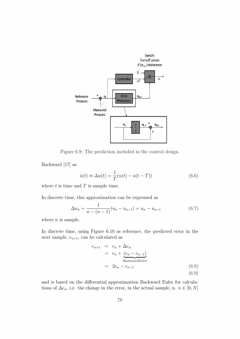
Error PredictionController uu*0 Switch:Turn off valvesif |ek+1|<tolerance

Reference Pressure MeasuredPressure ek+1ek+ -z

1ek ek-1 + + ek+1Figure 6.9: The prediction included in the control design.

Backward [17] as

u(t) ≈ ∆u(t) =1

T(u(t)− u(t− T )) (6.6)

where t is time and T is sample time.

In discrete time, this approximation can be expressed as

∆un =1

n− (n− 1)(un − un−1) = un − un−1 (6.7)

where n is sample.

In discrete time, using Figure 6.10 as reference, the predicted error in thenext sample, en+1, can be calculated as

en+1 = en + ∆en

= en + (en − en−1)︸︷︷︸BackwardEuler

= 2en − en−1 (6.8)

(6.9)

and is based on the differential approximation Backward Euler for calcula-tions of ∆en, i.e. the change in the error, in the actual sample, n. n ∈ [0, N ]

78

where N is the total number of samples. The same principle is used to predictthe error in the two next samples, en+2, and is given by

en+2 = en+1 + ∆en+1

= en+1 + en+1 − en︸︷︷︸BackwardEuler

= 2en+1 − en

= 3en − 2en−1 (6.10)

en

en-1

en+1

n

e

n-1 n n+1 n+2

en+2

en+1

en

∆∆

Figure 6.10: Error in previous, actual and next sample, based on the predic-tion calculation.

A drawback with the prediction part is that it is just an approximation of theerror in the future. If this assumption is wrong, the valves may deactivateat wrong moments, e.g. too early. Then the controller has to re-regulate theerror so that the reference is reached, and can in some occasions result in afurther time delay. The advantage is that the oscillations on the output canbe prevented.

6.5.3 Improved control using non-linear control

An additional non-linear control approach has been investigated in order toboost up the control signal in cases where the valve response is too weak, e.gif the prediction has resulted in a too early inactivation of the valves. Theboost is done by including an extra integrator which is activated only whenthe there is no response in the output pressure and as long as the error islarger than the accepted error tolerance. The method is used in simulationsand experiments in this thesis due to good results, but is investigated morein detail in the parallel work [13].

79

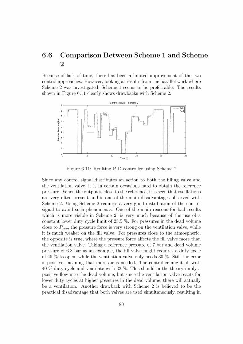
6.6 Comparison Between Scheme 1 and Scheme

2

Because of lack of time, there has been a limited improvement of the twocontrol approaches. However, looking at results from the parallel work whereScheme 2 was investigated, Scheme 1 seems to be preferrable. The resultsshown in Figure 6.11 clearly shows drawbacks with Scheme 2.

0 5 10 15 20 250

1

2

3

4

5

6

7

8

9

Time [s]

Rel

ativ

e P

ress

ure

[Bar

]

Control Results − Scheme 2

PchPref

Figure 6.11: Reulting PID-controller using Scheme 2

Since any control signal distributes an action to both the filling valve andthe ventilation valve, it is in certain occasions hard to obtain the referencepressure. When the output is close to the reference, it is seen that oscillationsare very often present and is one of the main disadvantages observed withScheme 2. Using Scheme 2 requires a very good distribution of the controlsignal to avoid such phenomenas. One of the main reasons for bad resultswhich is more visible in Scheme 2, is very much because of the use of aconstant lower duty cycle limit of 25.5 %. For pressures in the dead volumeclose to Psup, the pressure force is very strong on the ventilation valve, whileit is much weaker on the fill valve. For pressures close to the atmospheric,the opposite is true, where the pressure force affects the fill valve more thanthe ventilation valve. Taking a reference pressure of 7 bar and dead volumepressure of 6.8 bar as an example, the fill valve might requires a duty cycleof 45 % to open, while the ventilation valve only needs 30 %. Still the erroris positive, meaning that more air is needed. The controller might fill with40 % duty cycle and ventilate with 32 %. This should in the theory imply apositive flow into the dead volume, but since the ventilation valve reacts forlower duty cycles at higher pressures in the dead volume, there will actuallybe a ventilation. Another drawback with Scheme 2 is believed to be thepractical disadvantage that both valves are used simultaneously, resulting in

80

a more frequently use of the valves, causing more wear of the valves. Thisis believed to be better for Scheme 1 and is important to consider whenrobustness of the proportional valve used in current retarder system and thesystem using on/off valves is to be compared. Using Scheme 2, is howeverbelieved to allow for larger valve orifices, making it possible to have a fasterfilling and ventilation response, which is not possible having a smaller orifice.This is explained by the fact that while one of the valves are acting, the othervalve can at the same time be activated preventing the response to be toofast when the error is so small that a slower response is needed to reach thereference.

81

Chapter 7

Conclusions and Future work

7.1 Conclusions

The Master’s Thesis aimed to investigate if today’s system that uses a pro-portional valve to control the air pressure in the Retarder, could be replacedby two on/off solenoid valves and a pressure chamber with a pressure sensor,in order to reduce costs and improve the system robustness. The idea was tolet one filling valve and one ventilation valve together with a pressure supply,build a pressure in the chamber, determining an oil pressure in the Retarderand eventually the braking torque in the truck.

A model of the system was obtained, but validation of the model showsthat the quality of the model is not optimal. The model contains someweaknesses that in future work could further be investigated and improvedby including the probably missing dynamics in the electronic control unitand the magnetic properties. The modelled current and pressure correspondwell to the real current and pressure for high duty cycles as input signals.For low duty cycles, the modelled current differs from the real current in theamplitude and causes the valves to be closed for longer time than in reality,and thereby a longer time to fill or ventilate air from the chamber.

To control the valves, two different controllers were investigated. A con-trol approach using a pulse width modulated pulsing scheme where the fillvalve acts for positive errors and the ventilation valve acts for negative errors(Scheme 1) seemed to give best results, and was designed in this Master’sThesis. Simulations prove the excellence of using a regular PID controlleron the system. Results from tests on the real system have shown a strongpotential in having two on/off valves controlling the retarder, with addi-tional integral boosting action and a method for reducing overshoots usingerror prediction. With further research, the method using Scheme 1 can be

83

considered to be a promising approach.Another approach, Scheme 2, which was investigated in the parallel work [13]

let the filling valve and the ventilation valve act simultaneously. This wasthought to be a faster and more controlled way to control the air pressure,with the intention that a bigger valve orifice could be used to get a fasterresponse and even have the opportunity to reduce the action of one valve byletting the other valve counteract at the same time. A poor control perfor-mance was achieved using Scheme 2 and showed at the same time a worserobustness taking life-span into consideration.

Experiments have been done on physical models of the system with differentdimensions in order to determine proper parameters for volume of the cham-ber and orifice of the valve. Results show that a proper total dead volume(total volume in the system including volume in the valve housing, chamberand regulating valve), in order to fulfill actual time constraints and controlperformance, should be a bit less than 75 cm3 using an orifice of 1.9 mm.

7.2 Future Work

The Master’s Thesis has highlighted several aspects with on/off control onthe Retarder, and has investigated how certain parts can be improved puttingmore research and time into modeling and control of Retarder using on/offvalves. Improvements has not been performed in this work because of lackof time. However, recommendations based on investigation and experiencecan be given to future developers.

In order to make a better system model, more complexity from the elec-trical drives in the ECU could be included, so that the modelled currentbehaves more like the real current. The magnetic valve properties could beinvestigated in more detail, where the magnetic field in the iron core in thevalves could be included. An improved model can be used to make a modelbased controller. A model based controller have the advantage that the sys-tem properties may be included in the design, resulting in more freedomchoosing control strategies and may improve the control performance.

It has been observed that depending on the pressure in the dead volume,different duty cycles are needed to start opening the valves. Which has beenseen, a common problem causing time delays in Scheme 1 and oscillationsin Scheme 2, is the constant lower duty cycle limit of 25.5 % used in thedistributor. In future work, this lower duty cycle limit should be implementedas a function of the actual pressure in the dead volume where the lower duty

84

cycle limit varies between 25.5 % and 51.5 %. In this way eventual timedelays in the integral part and oscillations in the output pressure can bereduced.

85

Bibliography

[1] Scania CV AB, Sodertalje. 2008. http://www.scania.com

[2] Kleinknecht Automotive GMBH. 2008. http://www.kleinknecht.com/

[3] L.Ljung, T.Glad. ”Modellbygge och Simulering”. 2004.

[4] J.Ma, H.Schock, U.Carlsson, A.Hoglund and M.Hedman, ”Analysis andModeling of an Pneumatic Hydraulic Valve for an Automotive Engine”,SAE International, 2006-01-0042, 2006 SAE World Congress Detroit,MI, April 3-6, 2006.

[5] G.Petersson. ”Teoretisk Elektroteknik - Stationara fenomen”. 2004.

[6] G.Petersson. ”Teoretisk Elektroteknik - Elektromagnetsism”. Maj 2002.

[7] C.Nordling, J.Osterman. ”Physics Handbook for Science and Engineer-ing”. 1999.

[8] K-E.Rydberg. ”Basic theory for Pneumatic System Design”. Linko pingUniversity. IKP, Fluid and Mechanical Engineering Systems. 1997.

[9] R.A.Serway, J.W.Jewett. ”Physics for Scientists and Engineers withModern Physics”. 6th Edition. 2004.

[10] B.Eriksson, J. Wikander. Lecture notes in MF2007. Dynamics and Mo-tion Control. 2007.

[11] John C. Kayser, Robert L. Shambaugh. ”Discharge Coefficients for Com-pressible Flow Through Small-Diameter Orifices and Convergent Noz-zles”. Chemical Engineering Science, Vol 46, No 7, pp. 1697-1711, 1991.

[12] K.Hakansson, M.Johnson. ”Modeling and Control of an Electro Pneu-matic Actuator System Using On/Off Valves”. Department of ElectricalEngineering. Linkoping University, 2007.

86

[13] M.J.Tehrani. Pressure Control of a Pneumatic Actuator Using On/OffSolenoid Valves. The School of Electrical Engineering. The Royal Insti-tute of Technology. 2008.

[14] T. Noritsugu. ”Development of PWM Mode Electro-Pneumatic Ser-vomechanism, Part II: Position Control of a Pneumatic Cylinder”. J.of Fluid Control, 67:7-28, 1987.

[15] R.B.Van Varseveld, G.M.Bone. ”Accurate Position Control of a Pneu-matic Actuator Using On/Off Solenoid Valves”. Proc. of the IEEE Int.Conf on Rob. and Aut., 1196-1200. April 1997.

[16] L.Krause, J.Larsson. ”Konceptstudie: Tryckstyrning Av Hydrody-namisk Broms”. Master’s Thesis. Linkoping University. Linkoping, 2004.

[17] L.Ljung, T.Glad. ”Reglerteknik: Grundlaggande teori”. PreliminaryEdition, 2005.

[18] L.Ljung, T.Glad. ”Reglerteori. Flervariabla och Olinjara Metoder”. 2ndEdition, 2003.

87

Appendix A

Appendix

A.1 Linearization

According to [10] a nonlinear system x = f (x, u) can be linearized aroundsome operating point x0, u0 by considering a neighborhood around theoperating point and approximating the nonlinear model with a truncatedTaylor series. This is done by setting x = x0 + ∆x, u = u0 + ∆u andy = y0 + ∆y, then

x = f (x, u) + ∂f∂x

∣∣x=x0

u=u0

∆x + ∂f∂u

∣∣x=x0

u=u0

∆u

y = g (x, u) + ∂g∂x

∣∣x=x0

u=u0∆x + ∂g

∂u

∣∣x=x0

u=u0∆u

(A.1)

The system has been thought to be in equilibrium either when both valvesare deactivated, when only one of the valves is fully open, or when bothvalves are fully open. The equilibrium when both valves are fully activatedhas been considered. In this case the PWM signal is set to 100 % DC onboth valves, and the pressure will reach a constant pressure unless there areany disturbances disturbing the valves. The steady position will correspondto the current when the coil is fully charged, and will probably be outsidethe physical position limitation in the valve, i.e. outside the walls. In thisequilibrium, the velocity will be zero.

89

A.1.1 Fill valve and Ventilation valve are both acti-vated

Equilibrium points:x0

1 x02 x0

3 x04

x05 x0

6 x07

Linearized Model:

∆x = A∆x + B∆u

∆y = C∆x + D∆u

∆x =

x1

x2

x3

x4

x5

x6

x7

and ∆x =

x1

x2

x3

x4

x5

x6

x7

(A.2)

A = ∂f∂x

∣∣x=x0

u=u0B = ∂f

∂u

∣∣x=x0

u=u0

C = ∂f∂x

∣∣x=x0

u=u0D = ∂f

∂x

∣∣x=x0

u=u0

(A.3)

90

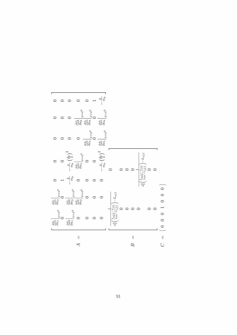
A=

∂f1

∂x1

∣ ∣ ∣ x=

x0

∂f1

∂x2

∣ ∣ ∣ x=

x0

00

00

0

00

10

00

0∂f3

∂x1

∣ ∣ ∣ x=

x0

∂f3

∂x2

∣ ∣ ∣ x=

x0−

bm

p−

π mp

( d0 2

) 20

00

0∂f4

∂x2

∣ ∣ ∣ x=

x0

0∂f4

∂x4

∣ ∣ ∣ x=

x0

0∂f4

∂x6

∣ ∣ ∣ x=

x0

0

00

00

∂f5

∂x5

∣ ∣ ∣ x=

x0

∂f5

∂x6

∣ ∣ ∣ x=

x0

0

00

00

00

1

00

0−

π mp

( d0 2

) 2∂f7

∂x5

∣ ∣ ∣ x=

x0

∂f7

∂x6

∣ ∣ ∣ x=

x0−

bm

p

B=

1

x0 2

(L

of

f−

Lon

xon−

xof

f

) −Lof

f

0

00

00

00

01

x0 6

(L

of

f−

Lon

xon−

xof

f

) −Lof

f

00

00

C=

[ 00

01

00

0]

91

wher

e∂f 1

∂x

1

∣ ∣ ∣ ∣ x=

x0

=−

R

x0 2

( Lof

f−L

on

xon−x

of

f

) −L

off

∂f 1

∂x

2

∣ ∣ ∣ ∣ x=

x0

=−

(u0 1−

Rx

0 1)( L

of

f−L

on

xon−x

of

f

)

( x0 2

( Lof

f−L

on

xon−x

of

f

) −L

off

) 2

∂f 3

∂x

1

∣ ∣ ∣ ∣ x=

x0

=µ

0A

pN

2x

0 1

mp(x

off−

x0 2)2

∂f 3

∂x

2

∣ ∣ ∣ ∣ x=

x0

=µ

0A

pN

2(x

0 1)2

mp(x

off−

x0 2)3−

ks

mp

∂f 4

∂x

2

∣ ∣ ∣ ∣ x=

x0

=

√R

gasT

air

Vch

d0πC

d,s

upP

sup

√k

(2

k+

1

)k+

1k−

1

∂f 4

∂x

4

∣ ∣ ∣ ∣ x=

x0

=−

√R

gasT

air

Vch

d0πC

d,v

entx

0 6

√ √ √ √2k

k−

1

( (P

atm

x0 4

)2 k

−( P

atm

x0 4

)k+

1k

)+

√2k

k−1

( −2 k

(P

2 k atm

(x0 4)2

+k

k

)+

k+

1k

( Pa

tm

x0 4

k+

1k

))

2√( P

atm

x0 4

)2 k−

( Pa

tm

x0 4

)k+

1k

x0 4

∂f 4

∂x

6

∣ ∣ ∣ ∣ x=

x0

=−

√R

gasT

air

Vch

d0πC

d,v

entx

0 4

√ √ √ √2k

k−

1

((P

atm

x0 4

2 k

)−

(P

atm

x0 4

k+

1k

))

92

∂f 5

∂x

5

∣ ∣ ∣ ∣ x=

x0

=−

R

x0 6

( Lof

f−L

on

xon−x

of

f

) −L

off

∂f 5

∂x

6

∣ ∣ ∣ ∣ x=

x0

=−

(u0 1−

Rx

0 5)( L

of

f−L

on

xon−x

of

f

)

( x0 6

( Lof

f−L

on

xon−x

of

f

) −L

off

) 2

∂f 7

∂x

5

∣ ∣ ∣ ∣ x=

x0

=µ

0A

pN

2x

0 5

mp(x

off−

x0 6)2

∂f 7

∂x

6

∣ ∣ ∣ ∣ x=

x0

=µ

0A

pN

2(x

0 5)2

mp(x

off−

x0 6)3−

ks

mp

93

Documents

Modeling and Control of Retarder using On/O Solenoid Valves572695/FULLTEXT01.pdf · Modeling and control of Retarder is a work provided by Scania as a part of the development and