University of Tennessee, Knoxville University of Tennessee, Knoxville

TRACE: Tennessee Research and Creative TRACE: Tennessee Research and Creative

Exchange Exchange

Masters Theses Graduate School

5-2018

Modeling and analysis of variable reactive power limits of a Modeling and analysis of variable reactive power limits of a

Doubly Fed Induction Generator (DFIG) used in variable speed Doubly Fed Induction Generator (DFIG) used in variable speed

wind turbines wind turbines

Jonathan Devadason University of Tennessee, jdevadas@vols.utk.edu

Follow this and additional works at: https://trace.tennessee.edu/utk_gradthes

Recommended Citation Recommended Citation Devadason, Jonathan, "Modeling and analysis of variable reactive power limits of a Doubly Fed Induction Generator (DFIG) used in variable speed wind turbines. " Master's Thesis, University of Tennessee, 2018. https://trace.tennessee.edu/utk_gradthes/5073

This Thesis is brought to you for free and open access by the Graduate School at TRACE: Tennessee Research and Creative Exchange. It has been accepted for inclusion in Masters Theses by an authorized administrator of TRACE: Tennessee Research and Creative Exchange. For more information, please contact trace@utk.edu.

To the Graduate Council:

I am submitting herewith a thesis written by Jonathan Devadason entitled "Modeling and

analysis of variable reactive power limits of a Doubly Fed Induction Generator (DFIG) used in

variable speed wind turbines." I have examined the final electronic copy of this thesis for form

and content and recommend that it be accepted in partial fulfillment of the requirements for the

degree of Master of Science, with a major in Electrical Engineering.

Hector A. Pulgar, Major Professor

We have read this thesis and recommend its acceptance:

Seddik M. Djouadi, Kai Sun

Accepted for the Council:

Dixie L. Thompson

Vice Provost and Dean of the Graduate School

(Original signatures are on file with official student records.)

Modeling and analysis of variable

reactive power limits of a Doubly Fed

Induction Generator (DFIG) used in

variable speed wind turbines

A Thesis Presented for the

Master of Science

Degree

The University of Tennessee, Knoxville

Jonathan Devadason

May 2018

c© by Jonathan Devadason, 2018

All Rights Reserved.

ii

Dedicated to my dear parents Dr. Reenie Devadason and Mr.Joseph Devadason, my little

brother Moses Devadason and my grandmother, Late.Mrs.Jessie Muthumani...

iii

Acknowledgments

I express my deepest thanks to my Higher Power without Whom this task would have been

impossible.

I would like to thank Dr. Hector Pulgar - Painemal for his excellent guidance in this

work. I would also like to thank Dr. Kai Sun, Dr. Seddik Djouadi and Dr. Fangxing Li for

all their encouragement and support in this endeavor.

I am greatly indebted to my parents Dr.Reenie Devadason and Mr. Joseph Devadason

for their wonderful support and encouragement to follow my passion. I also want to mention

my friends in UT and my ministers Ben Winder, Scott Claybrook and Susan Tatum for

helping me stay motivated through the entire duration of this thesis.

Finally, I would like to express my deepest appreciation to the staff of Ebenezer counseling

services and Blount Memorial hospital for the care they provided during the most crucial

part of this research.

iv

Abstract

In this thesis, the mathematical modeling of variable reactive power limits for a Doubly Fed

Induction Generator (DFIG) based on its capability curves is presented. Reactive power

limits have been adjusted dynamically based on the capability curves when the system was

subjected to a disturbance. This ensures that the operation of the DFIG is always within

safe limits and utilizes the available capability of the DFIG to improve the performance of

the system.

The small signal stability of the system is studied by considering the load as a variable

parameter. The differential-algebraic model of the DFIG, synchronous generators and their

associated controllers and the power system network is linearized and bifurcation analysis

considering the load as the bifurcation parameter has been performed. The PV curves, the

stator and rotor current magnitudes, and the eigenvalue trajectories are plotted as the load

is varied. Time domain simulations are performed to observe the change in stator and rotor

currents when the system is subjected to a load change and a change in the wind speed.

The system considered for testing is the IEEE 9 bus system which is modified to include a

wind farm consisting of 5 wind turbines. The variable reactive power limits are implemented

in the reactive power controller of the DFIG and the performance of the system is compared

to that of the system with fixed limits in the reactive power controller. From the bifurcation

analysis, it was observed that the stator and rotor currents were at the maximum limits

when the lower and upper limits of the controller were reached. Also, the Hopf bifurcation

was found to occur at a lower load level compared to the system with fixed reactive power

limits. From the time domain simulations, it was observed that the stator and rotor currents

did not exceed the maximum limits in the system with variable reactive power limits when

the system was subjected to a change in the load and a change in the wind speed. Hence,

v

the problem of over/under estimating the reactive power capability of the DFIG based wind

farm was avoided.

vi

Table of Contents

1 Introduction 1

1.1 Types of wind turbines . . . . . . . . . . . . . . . . . . . . . . . . . . . . . . 1

1.2 Wind turbines participation in frequency and voltage regulation . . . . . . . 2

1.3 State of the art . . . . . . . . . . . . . . . . . . . . . . . . . . . . . . . . . . 3

1.4 Literature review . . . . . . . . . . . . . . . . . . . . . . . . . . . . . . . . . 4

1.5 Organization of the thesis . . . . . . . . . . . . . . . . . . . . . . . . . . . . 5

2 Mathematical modeling of DFIG controllers 6

2.1 Control of active and reactive power . . . . . . . . . . . . . . . . . . . . . . 8

2.1.1 Active power control . . . . . . . . . . . . . . . . . . . . . . . . . . . 8

2.1.2 Reactive power control . . . . . . . . . . . . . . . . . . . . . . . . . . 8

2.1.3 Supervisory control . . . . . . . . . . . . . . . . . . . . . . . . . . . . 9

2.2 Participation of a DFIG in frequency regulation . . . . . . . . . . . . . . . . 10

2.2.1 Inertial response of DFIG wind turbines . . . . . . . . . . . . . . . . 11

2.2.2 Frequency regulation through pitch control of wind turbines . . . . . 11

3 Mathematical modeling of variable reactive power limits of the DFIG 13

3.1 Capability curves . . . . . . . . . . . . . . . . . . . . . . . . . . . . . . . . . 13

3.2 Mathematical modeling of reactive power limits . . . . . . . . . . . . . . . . 16

3.2.1 Modeling of rotor voltage limits of the DFIG considering the losses . 16

3.2.2 Reactive power limits neglecting losses in the DFIG circuit . . . . . . 19

4 Results and analysis 22

vii

4.1 Linearization of the power system model . . . . . . . . . . . . . . . . . . . . 22

4.2 Simulation results . . . . . . . . . . . . . . . . . . . . . . . . . . . . . . . . . 24

4.2.1 Analysis of PV curves . . . . . . . . . . . . . . . . . . . . . . . . . . 24

4.2.2 Variation of stator and rotor currents with load . . . . . . . . . . . . 26

4.2.3 Results of time domain simulations . . . . . . . . . . . . . . . . . . . 28

5 Conclusions 35

5.1 Inference drawn from the study . . . . . . . . . . . . . . . . . . . . . . . . . 35

5.2 Future work . . . . . . . . . . . . . . . . . . . . . . . . . . . . . . . . . . . . 36

Bibliography 37

Appendices 42

A Derivation of reactive power limits based on rotor current limit . . . . . . . . 43

B Derivation of reactive power limits based on stator current limit . . . . . . . 45

Vita 47

viii

List of Tables

4.1 Hopf bifurcation points of systems A and B . . . . . . . . . . . . . . . . . . 27

ix

List of Figures

2.1 Control system of the DFIG . . . . . . . . . . . . . . . . . . . . . . . . . . . 7

2.2 Modified representation of the voltage controller . . . . . . . . . . . . . . . . 9

2.3 Control scheme to provide frequency regulation through inertial response . . 11

2.4 Control scheme to provide frequency regulation through pitch control . . . . 11

3.1 Equivalent circuit of a DFIG . . . . . . . . . . . . . . . . . . . . . . . . . . . 13

3.2 Capability curves for a supersynchronous slip of 0.23 . . . . . . . . . . . . . 15

3.3 Capability curves for a supersynchronous slip of 0.25 . . . . . . . . . . . . . 15

4.1 Test system considered for study . . . . . . . . . . . . . . . . . . . . . . . . 23

4.2 PV curve with fixed reactive power limits in the DFIG . . . . . . . . . . . . 25

4.3 PV curve with variable reactive power limits in the DFIG . . . . . . . . . . . 26

4.4 Stator and rotor currents for the system with fixed reactive power limits . . 27

4.5 Stator and rotor currents for the system with variable reactive power limits . 28

4.6 Variation of stator and rotor currents with time for a load step for system A 29

4.7 Variation of stator and rotor currents with time for a load step for system A

with inertial control . . . . . . . . . . . . . . . . . . . . . . . . . . . . . . . . 30

4.8 Variation of stator and rotor currents with time for a load step for system B 31

4.9 Variation of stator and rotor currents with time for a load step for system B

with inertial control . . . . . . . . . . . . . . . . . . . . . . . . . . . . . . . . 32

4.10 Variation of stator and rotor currents with time for a change in the wind speed

for system A . . . . . . . . . . . . . . . . . . . . . . . . . . . . . . . . . . . . 33

4.11 Variation of stator and rotor currents with time for a change in the wind speed

for system B . . . . . . . . . . . . . . . . . . . . . . . . . . . . . . . . . . . . 34

x

Chapter 1

Introduction

Nowadays, the world is moving towards clean forms of energy. This is mainly due to the

global warming issues due to the emission of CO2 into the atmosphere and one of the main

contributors to this are the conventional power plants.This would lead to other problems like

acid rain [1] and greenhouse effect [2]. Also,there is a depletion of fossil fuels in the earth [3].

All these reasons have led to the increase in the deployment of renewable energy resources

[4]. Wind is one of the cleanest forms of energy.Also, the cost of production of energy from

wind has come down in the recent years [5].

1.1 Types of wind turbines

Wind turbines are classified into three types - Fixed speed (Type A), semi variable speed

(Type B) and variable speed wind turbines (Type C) [6],[7], [8]. The fixed speed wind

turbines are usually based on Squirrel Cage Induction Generators (SCIGs) which provide

output only through the stator winding. It requires a grid connected SCIG coupled to the

wind turbine through a gear box. Because of the coupling to the grid, the speed varies over

a very small range (usually around 1%), hence commonly known as fixed speed system. At

speeds other than the rated wind speed, fluctuations in the wind speed leads to pulsations

in the torque (power) which leads to grid voltage fluctuations and strain on the gear box.

Also, these generators always consume reactive power from the grid and hence, capacitors

need to be installed to compensate for this.

1

In semi - variable speed operation, some of the generator shaft power is dissipated in

the rotor, the pulsations in the power is reduced under fluctuating wind conditions. The

variation of the rotor resistance with the slip is maintained constant which keeps the rotor

current and the airgap power constant.

Variable speed wind turbines are more advantageous when compared to the other two

technologies. This makes use of a wound rotor induction generator. Bidirectional power

flow through the rotor circuit is achieved by utilizing an ac-dc-ac converter between the

slip ring terminals and the grid. The converter can be fully or partially rated. Full rated

converters are more expensive than partially rated ones and hence, sparingly used. Here, we

limit ourselves to the study of a wind turbine with partially rated converters as this is less

expensive. The rating of the converter is usually 25 - 30% of the rating of the machine. The

arrangement consists of an induction generator with a back to back converter connecting the

grid and the rotor circuit. This is called ’Doubly Fed Induction Generator (DFIG)’.

1.2 Wind turbines participation in frequency and volt-

age regulation

Modern grid codes demand wind power plants to participate in frequency regulation [9], [10].

This leads to increased real power generation for short amounts of time requiring regulation

of active power.

It is advantageous to maintain the voltage at a remote bus at a reference value using

a supervisory control mechanism which generates the reactive power needed to regulate

the voltage at the remote bus [11]. But with the load in the system increasing and the

wind turbines also participating in frequency regulation, the availability of reactive power

obtained from the DFIG based wind turbines is limited. In the existing literature, the DFIG

is implemented with either limits on the individual PI controllers controlling the reactive

power limits, d component of the rotor current and the d component of the rotor voltage

or just having a supervisory control mechanism with no limits implemented in the DFIG.

2

In this thesis, two different models of reactive power limits based on the capability curve

equations are presented.

1.3 State of the art

The voltage at a bus in a power system can be regulated by controlling the rotor and the

grid side converters [12]. In order to do this, there should be sufficient amount of reactive

power capability from the wind farm. The rotor angle stability of the power system can be

improved by controlling the terminal voltage of the DFIG [13]. Additional reactive power

is available from the DFIG based wind farm when it is operated based on the capability

curves [14].It is possible to control the DFIG based wind turbine so it can provide voltage

regulation, frequency regulation and oscillation damping by controlling the magnitude and

angle of the rotor flux [15]. The reactive power capability of the wind farm depends on

the operating slip and the real power output of the wind farms which in turn depends on

the wind speed. Hence, there is a possibility of over/under estimating the reactive power

capability of the wind farms which may lead to unsafe operation due to the violation of

operating limits.

The availability of additional reactive power from a DFIG based wind farm by utilizing the

capability curve of the machine is described in reference[16]. Here, only the underutilization

of reactive power capability of wind farms by operating at a fixed power factor has been

discussed. The effects of wind speed variations and the impact of the availability of

additional reactive power on the small signal stability of the system has not been analyzed.

The control of DFIG based wind turbine so as to provide frequency regulation, oscillation

damping and voltage control is described in reference [15]. A Flux Magnitude and Angle

Controller (FMAC) is used to provide the control mechanism by adjusting the rotor flux

vector magnitude and angle. The effect on the reactive power output of the DFIG is not

discussed here.

3

1.4 Literature review

Reference [17] describes the capability curves of the DFIG and a main observation made is

that under normal operating values of slip, the stator current plays a limiting role in the

absorption of reactive power and the rotor current limits the production of reactive power.

In reference [18], the capability curves of the DFIG have been obtained considering the

limitations in converter currents, junction temperature and saturation effects. But in this

thesis, the non linearities with respect to saturation and temperature effects have not been

considered for the sake of simplicity.

The steady state model of the DFIG, the coupling effects between the q-component of

the rotor current and the active power as well as the d-component of the rotor current and

the reactive power and the capability curves of the DFIG have been described in reference

[19]. The steady state model described in this article is adopted for the study conducted in

this thesis.

The requirements which have to be met when wind farms are connected to the grid

with respect to real and reactive power control, voltage control and frequency control and

supporting grid voltage under the occurrence of faults have been discussed in references [20]

and [9]. The participation of DFIG based wind farms in regulating real power and frequency

will affect the reactive power capability available for the controlling the voltage.

The mathematical modeling of induction machines based on the reference frame theory is

explained in reference [21] which has been applied in this study to derive the mathematical

model of the DFIG.

The mathematical model of DFIG based wind farms and the control schemes has been

presented in reference [22]. The data of the 3.6 MVA wind farm in this article has been used

for the DFIG based wind turbines in this thesis. The mathematical modeling of a DFIG,

pitch angle controller, terminal voltage controller and a speed controller has been presented

in reference [23] based on which the DFIG was initialized for bifurcation analysis and time

domain simulations in this study.

The ability of the DFIG to provide frequency regulation through inertial response by

utilizing additional control loops is discussed in references [24] and [25].

4

The application of bifurcation theory to power systems has been discussed in reference

[26]. The different kinds of bifurcations which might occur in a power system and the issues

related to loading are summarized in reference [27]. The load at a bus is considered as a

bifurcation parameter which has been adapted in this thesis as well.

The utilization of FACTS devices to eliminate bifurcations in the power system is

described in reference [28]. The comparison of the performance of different FACTS devices in

eliminating bifurcations is presented in reference [29]. With the utilization of the capability

curves in the DFIG, the reactive power availability will be reduced during periods of high

active power production and under disturbances when the DFIG participates in frequency

regulation. A co-ordinated control between the DFIG and the FACTS devices can be

explored as an extension of the work done in this thesis.

1.5 Organization of the thesis

This thesis is organized as follows: The mathematical model of the wind turbine controllers

are presented in chapter 2. Chapter 3 presents the mathematical modeling of the reactive

power limits of the DFIG, chapter 4 describes the test system considered and the results and

analysis of the same. The conclusion is presented in chapter 5.

5

Chapter 2

Mathematical modeling of DFIG

controllers

The mathematical model used in this thesis for the DFIG based wind farm is based on

reference [11].The stator and rotor transients are assumed to be very fast and hence, they

are neglected. The detailed mathematical model of the DFIG can be found in reference [30].

The wind turbine shaft is modeled by a single mass. The mathematical models of the

wind turbine and the shaft sections can be found in reference [11]. In this study, stator

flux orientation has been assumed for the DFIG which allows independent control real and

reactive power. There are different controllers in the DFIG to control voltage, active power,

reactive power and inertial and pitch controllers depending on whether the DFIG participates

in frequency regulation or not. The mathematical models of the different controllers have

been derived in the following sections.

6

REAL POWER CONTROLLER

Vqr

REACTIVE POWER CONTROLLER

KP2 +KI2s

KP1 +KI1s

IqrefF (ωr)

Optimaltracking

Prefωr

IqrP

--

++

DFIG

KP4 +KI4s

KP3 +KI3s

VdrIdrefQrefQord

IdrQ

--

++

QMAX

QMIN

ωr

P

VD

QMIN

QMAX

Q limit calculator based on capability curves

KPV + KIVs

Vref

V

+-

1fN

11+sTc

SUPERVISORY CONTROLLER

Figure 2.1: Control system of the DFIG

777

2.1 Control of active and reactive power

The block diagram for the active and reactive power control and supervisory control of the

DFIG is shown in figure 2.1.

2.1.1 Active power control

The active power is regulated at the reference value Pref which is obtained from the Maximum

Power Point Tracking curve (MPPT ) which has been approximated by the equation

Pref = Cω3r (2.1)

where C is a parameter which is tuned [31]. The resulting error in the active power is

processed by a PI controller which generates the reference signal corresponding to the q-

component of the rotor current (Iqref ). The error in the q-component of the rotor current is

processed by a second PI controller which generates the signal Vqr which is the q-component

of the rotor voltage which is injected into the rotor to control active power. The state and

algebraic equations corresponding to the active power controller are derived as shown below:

x1 = KI1(Pref − P ) (2.2)

x2 = KI2(Iqref − Iqr) (2.3)

Iqref = KP1(Pref − P ) + x2 (2.4)

Vqr = KP2(Iqref − Iqr) (2.5)

2.1.2 Reactive power control

The reactive power reference is obtained from the supervisory voltage controller. The error

in the reactive power is processed by a PI controller which generates the d-component of the

rotor current (Idref ). The difference in Idref and the d-component of the rotor current (Idr)

is processed by a second PI controller which dictates the d-component of the voltage (Vdr)

8

to be injected into the rotor to control the reactive power. The equations pertaining to the

reactive power controller are given below:

x3 = KI3(Qref −Q) (2.6)

x4 = KI4(Idref − Idr) (2.7)

Idref = KP1(Qref −Q) + x3 (2.8)

Vdr = KP2(Idref − Idr) + x4 (2.9)

2.1.3 Supervisory control

The block diagram of the supervisory control is also shown in figure 2.1. It consists of a PI

controller, the input of which is the voltage error (Vref − V ).The output of this controller is

the reactive power which is needed to regulate the voltage of the remote bus at Vref . The

constant fN is fraction which indicates the total number of wind turbines under operation.

The reactive power reference is scaled by the factor 1fN

which is the reactive power reference

which has to be supplied to all the wind turbines. A first order block with time constant Tc is

considered to take into account, the communication delay between the supervisory controller

and the individual wind turbines [11].

KPV

− KPVKIV (sKPV +KIV

+ +

-y

Vref

-V

Figure 2.2: Modified representation of the voltage controller

The mathematical model of the PI controller controlling the voltage is represented as

shown in figure 2.2 so that the limits can be applied on the algebraic equation which

represents the reactive power reference [11]. This is done just for ease of computation.

The equations representing this are

9

H(s) = KPV +KIV

s(2.10)

Equation (2.10) can be expressed in the form

H(s) =H1(s)

1 +H1(s)H2(s)(2.11)

where

H1(s) = KPV (2.12)

H2(s) =−KIV

KPV (sKPV +KIV )(2.13)

The differential equations corresponding to the supervisory control are given below:

y = −KIV

KPV

y − KIV

K2PV

(2.14)

˙Qord =1

TcfNQc −

1

TcQord (2.15)

where

Qc = KPV (Vref − V − y) (2.16)

2.2 Participation of a DFIG in frequency regulation

In this section, two control schemes of the DFIG to provide frequency regulation in the event

of a disturbance in the power system is presented [31].

10

Figure 2.3: Control scheme to provide frequency regulation through inertial response

2.2.1 Inertial response of DFIG wind turbines

The block diagram describing the control scheme to provide inertial response is shown in

figure 2.3. In this scheme, the kinetic energy stored in the wind turbine mass is used to

provide/absorb power when there is an under/over frequency condition. The function of the

washout filter is to ensure that the control acts only during the first moment of deviation.

2.2.2 Frequency regulation through pitch control of wind turbines

Figure 2.4: Control scheme to provide frequency regulation through pitch control

Figure 2.4 shows the control scheme adopted to provide frequency control by pitching the

blades of the wind turbine. The wind turbine is operated at a lower power at every point to

reserve an amount of margin which allows for controlling frequency by injecting/absorbing

power in the event of a disturbance. The disadvantage in this scheme is that the overall

11

power which is produced for a given wind speed is reduced which results in reduced revenue

for the owner of the wind farm.

12

Chapter 3

Mathematical modeling of variable

reactive power limits of the DFIG

In this chapter, the importance of capability curves and the mathematical modeling of

reactive power limits of the DFIG are presented. The main reason to implement variable

reactive power limits in the DFIG is because the reactive power depends on the real power

and slip of the machine. Since the operation of the wind turbine is slow compared to the

duration of the stator and rotor transients of the DFIG, the use of the capability curves to

compute the reactive power limits is justified.

3.1 Capability curves

Figure 3.1: Equivalent circuit of a DFIG

13

The equivalent circuit of the DFIG which is considered in this study is shown in figure

3.1. The two port network matrices for the circuit can be obtained asV as

Ias

=

−(Rs + jXs) jXm

−jXmRr

s+ jXr

︸ ︷︷ ︸

Z

IasIar

(3.1)

IasIar

= Y

V as

V ar

s

(3.2)

where

Y = Z−1 (3.3)

IasV ar

s

=

−1Rs+jXs

jXmRs+jXs

jXm

Rs+jXs

Rr

s+ jXr + Xm

2

Rs+jXs

︸ ︷︷ ︸

G

V as

Iar

(3.4)

V ar

s

Iar

=

Rrs

+jXr

jXm

(Rrs

+jXr)(Rs+jXs)+Xm2

jXm

1jXm

Rs+jXs

jXm

︸ ︷︷ ︸

B

V as

Iar

(3.5)

The DFIG has three operating limits - Rotor current limit,Stator current limit and Rotor

voltage limit. The capability curves of a DFIG for two different slips of operation are

represented in figures 3.2 and 3.3. In figure 3.2, it can be observed that the rotor current

limits the operation when reactive power is supplied to the grid and the stator current limits

the operation when reactive power is drawn from the grid. But when the slip increases, the

rotor voltage curve moves downward and limits the operation of the DFIG.

14

Figure 3.2: Capability curves for a supersynchronous slip of 0.23

Figure 3.3: Capability curves for a supersynchronous slip of 0.25

15

3.2 Mathematical modeling of reactive power limits

The reactive power limits related to the rotor voltage have been derived in the following

section. The losses in the DFIG are not neglected which makes the equation a bit complex.

The modeling of the limits neglecting the losses will be shown in section 3.2.2.

3.2.1 Modeling of rotor voltage limits of the DFIG considering

the losses

The elements of the admittance matrix Y (equations 3.2 and 3.3) can be represented as:

Y =

G11 + jB11 G12 + jB12

G21 + jB21 G22 + jB22

(3.6)

The complex power delivered by the stator is given by the equation

Ss = V asIas∗

(3.7)

where

V as = Vs (3.8)

V ar = Vrejβ (3.9)

The complex power at the stator Ss can also be expressed as

Ss = Ps + jQs (3.10)

where Ps and Qs is the real and reactive power delivered by the stator. Expressing V as and

Ias in terms of the elements of the Y matrix, Ps and Qs can be written as

Ps = G11Vs2 +

VsVrs

(G12 cos β −B12 sin β) (3.11)

Qs = −B11Vs2 − VsVr

s(G12 sin β +B12 cos β) (3.12)

16

The complex power delivered to the rotor is given by the equation

Sr = V arIar∗

(3.13)

If Pr and Qr represents the real and reactive power delivered to the rotor, the complex power

is also expressed as

Sr = Pr + jQr (3.14)

Similarly, expressing V ar and Iar in terms of the elements of the Y matrix, Pr and Qr can

be written as

Pr =Vr

2

sG22 + VsVr(G21 cos β +B21 sin β) (3.15)

Qr =−Vr2

sB22 + VsVr(G21 sin β −B21 cos β) (3.16)

The net real power generated is given by

PG = Ps − Pr (3.17)

The reactive power consumed by the rotor is supplied by the rotor side converter and hence,

the net reactive power generated is represented as

QG = Qs (3.18)

Substituting equations 3.11 and 3.15 in equation 3.17, PG can be written as

PG = k1 + A1 cos β +B1 sin β (3.19)

where

k1 = Vs2G11 − Vr2

sG22

A1 = VsVr(G12

s−G21)

17

B1 = −VsVr(B12

s+B21)

Now, equation 3.19 is rewritten as

PG − k1 = R1 cos(β − α) (3.20)

where

R1 =√A1

2 +B12

tanα = B1/A1

Let

(PG − k1)/R1 = cos γ (3.21)

Hence, equation 3.21 becomes

cos (β − α) = cos γ (3.22)

The solution for β from equation 3.22 is given by

β = α± γ (3.23)

Let β1 = α + γ

β2 = α− γ

(3.24)

The equation for the generated reactive power is expressed as

QG = −B11Vs2 − VsVr

s(G12 sin β +B12 cos β) (3.25)

where QG can be calculated for β1 and β2 which are functions of the slip and the real power

generated for that particular value of slip. Out of the two solutions for QG, the higher one

18

corresponds to the maximum value and the other value corresponds to the minimum value

of reactive power that can be produced.

3.2.2 Reactive power limits neglecting losses in the DFIG circuit

When the resistances Rs and Rr are neglected in the rotor circuit, the equations are much

simpler and are presented in this section. The impedance matrix Z is now modified as

Z =

−jXs jXm

−jXm jXr

(3.26)

Taking the inverse of equation 3.27, the admittance matrix Y has been derived as

Y =1

∆Z

jXr −jXm

jXm −jXs

(3.27)

where

∆Z = XsXr −X2m (3.28)

Following a similar procedure described in the section 3.2, the real and reactive power

delivered by the stator (Ps and Qs respectively) are given by the following equations:

Ps =Xm

s∆ZVsVr sin β (3.29)

Qs =Xm

s∆ZVsVr cos β − Xr

∆ZV 2s (3.30)

19

The real and reactive power absorbed by the rotor circuit (Pr and Qr) are given by the

equations

Pr =Xm

∆ZVsVr sin β (3.31)

Qr =Xs

∆Z

V 2r

s− Xm

∆ZVsVr cos β (3.32)

The net real power generated by the DFIG is given by the equations

PG = Ps − Pr (3.33)

PG =Xm

∆ZVsVr(

1

s− 1) sin β (3.34)

The reactive power generated by the DFIG considering that the reactive power consumed

by the rotor is supplied by the rotor side converter, hence the reactive power generated is

given by the equations

QG = Qs −Qr (3.35)

QG =Xm

s∆ZVsVr cos β − Xr

∆ZV 2s (3.36)

Squaring and adding equations 3.34 and 3.36 to eliminate β, the resulting equation is

Q2G + 2QGK1 +K2

1 − K22

s2+ (

PG1 − s

)2 = 0 (3.37)

where

K1 = Xm

∆ZVsVr

K2 = Xr

∆ZV 2s

Solving the quadratic equation 3.37, the reactive power generated is obtained as

QG = − Xr

∆ZV 2s ±

√(Xm

s∆ZVsVr)2 − (

PGs

1 − s)2 (3.38)

20

The higher value among the two solutions in equation 3.38 is the maximum reactive

power and the other value is the minimum amount of reactive power that can be generated

for a given slip and real power.

The real and reactive power equations considering the rotor current limit and the stator

current limit can be obtained using a similar procedure adapted in sections 3.2.1 and 3.2.2

and is presented in the Appendices A and B.

21

Chapter 4

Results and analysis

The reactive power limit models derived in chapter 3 are implemented in a 15 bus test

system comprising of 5 wind turbines as shown in figure 4.1 and the results are analyzed.

The mathematical model of the synchronous machine and its associated controllers can be

found in reference [32]. The load is considered to be a bifurcation parameter. This is because,

the system load plays an important role in the stability of the system. The effect of a step

change in the load and a change in the wind speed on the stator and rotor currents has been

studied using time domain simulations and the results are analyzed. The data of the system

is taken from reference [11].

4.1 Linearization of the power system model

The differential and algebraic equations which describe the dynamics of the system are

linearized around different operating points which are obtained by varying the load in a

certain bus in the system. The general form of the equations which describe the reactive

power limits is given as

Qlimit = f(VD, s, P ) (4.1)

22

Figure 4.1: Test system considered for study

where VD is the terminal voltage, s is the operating slip and P is the real power produced

for the given operating slip. The linearized form of equation 4.1 is expressed as

∆Qlimit = K1∆VD +K2∆wr +K3∆P (4.2)

where K1,K2 and K3 are the constants which are calculated for a particular operating point.

The equations are cast in matrix form

∆X = A∆X +B∆Y (4.3)

0 = C∆X +D∆Y (4.4)

Equation (4.4) can be rewritten as

∆Y = −D−1C∆X (4.5)

23

Substituting equation (4.5) in (4.3), the expression for ∆X is obtained as

∆X = (A−BD−1C)∆X (4.6)

Asys = A−BD−1C (4.7)

where Asys is the system matrix, the eigen values of which are calculated to study the stability

of the system.

4.2 Simulation results

The test system consists of three load buses namely buses 5, 6 and 8. Let the system with no

reactive power limits in the DFIG be denoted as system A and the system with reactive power

limits implemented in the DFIG be denoted as system B. The bifurcation analysis of the

system has been carried out considering the load at these buses as the bifurcation parameter

and the variation of the voltage at the point of common coupling (VPCC) is studied for the

system with fixed reactive power limits and variable reactive power limits in the controller for

reactive power. The time domain simulations are also performed in the system considering

a step change in the load at bus 5. Also, a change in the wind speed is considered from 11

to 12 m/s. The plots of the stator and rotor currents with respect to time are described.

4.2.1 Analysis of PV curves

The load considered in this system is a constant power factor load. The active and the

reactive power components of the load is increased in steps and the variation of the voltage

VPCC is plotted against the bifurcation parameter. In this case, it is the load at bus 6.

Figure 4.3 shows the variation of VPCC with the active power load for the system with

fixed reactive power limits. It is observed that between a load level of 10 MW to 82 MW,

the voltage is above the reference value (1 p.u) because the controller is operating at the

minimum reactive power limit. Between a load of 82 MW and 282 MW, the voltage is

regulated at 1 p.u and when the load exceeds 282 MW, the voltage starts dropping from 1

p.u because the controller operates at the lower reactive power limit.

24

Figure 4.2: PV curve with fixed reactive power limits in the DFIG

In figure 4.3, the variation of the voltage at the PCC is plotted against the active power

load at bus 6 when it is varied from 10 to 400 MW. The curve is of the same shape as that

of figure 4.2 but the difference is that between a load of 10 MW and 82 MW, the lower

limit of the supervisory control dictates the reactive power reference. The lower limit of the

supervisory controller is imposed by the stator current limit. Between a load of 82 MW and

250 MW, the voltage was regulated at 1 p.u and when the load exceeds 250 MW, the voltage

drops from 1 p.u because now, the reactive power limit is because of the rotor current limit.

From figures 4.2 and 4.3, it is clear that the estimated reactive power available to regulate

the voltage at the PCC was lower than what was actually available in the system.

25

Figure 4.3: PV curve with variable reactive power limits in the DFIG

4.2.2 Variation of stator and rotor currents with load

In figure 4.4, the variation of the stator and rotor currents with the active power load is

shown. From a loading level of 82 MW to 282 MW, the stator and rotor currents are within

the allowable limits but when the load is increased past 282 MW, the stator and rotor

currents surpass the maximum limits.

When figure 4.5 is observed, it can be observed that when the load is between 10 and

82, the stator current is at its maximum limit and between the load of 82 and 250, the rotor

current is at the maximum limit. Between 250 and 364, the system operates in the region

inside the capability curve and hence, the stator and rotor currents are well within the limits.

The load levels at which a Hopf bifurcation occurs for maintaining VPCC at 0.98 p.u and

1 p.u by performing the bifurcation analysis in systems A and B considering the loads at

buses 5, 6 and 8 as the bifurcation parameters are summarized in table .

26

Figure 4.4: Stator and rotor currents for the system with fixed reactive power limits

It is observed from table 4.1 that the Hopf bifurcation point is shifted when the system

has variable reactive power limits. This shift in the point for different values of reference

voltage at the PCC is due to the over/under estimation of the reactive power limits. The

location of the load bus where the bifurcation analysis is performed also determines the shift

in the bifurcation point when the system has variable reactive power limits based on the

capability curve. This has to do with the proximity of the load buses to the PCC.

Table 4.1: Hopf bifurcation points of systems A and B

Load bus Reference voltage System A System B

Bus 5 1 p.u 331 MW 317 MWBus 6 0.98 p.u 296 MW 304 MWBus 6 1 p.u 294 MW 316 MWBus 8 1 p.u 330 MW 326 MW

27

Figure 4.5: Stator and rotor currents for the system with variable reactive power limits

4.2.3 Results of time domain simulations

The system is subjected to a step change in the load at bus 5 and the results have been

discussed in this section.

Response to a step change in the load

Figure 4.6 shows the evolution of stator and rotor currents of the DFIG when system A

subjected to a step change in the load of 10% at time t = 0s. It is observed that the

rotor current exceeds the maximum allowable limit. Figure 4.7 shows the variation of the

stator and rotor currents of the DFIG in system A when the DFIG participates in frequency

regulation through inertial control. When the step change in the load is encountered, the

frequency of the system is supposed to drop. But with inertial response, the frequency nadir

is reduced as the DFIG releases the stored energy in the rotor. When this happens, the rotor

28

Figure 4.6: Variation of stator and rotor currents with time for a load step for system A

current increases. The rotor current is seen to exceed the maximum value when system A is

subjected to the disturbance which in this case is the step change in the load.

Figures 4.8 and 4.9 show the variation of stator and rotor currents of the DFIG when

system B is subjected to a step change in the load at bus 5. In this case, the stator and rotor

currents are within the limits. The rotor current is at the maximum limit as the load in the

system before the disturbance is at a level such that the system operates close to the rotor

current limit. When the DFIG participates in frequency regulation by providing inertial

response, the rotor current is at the limit and the stator current is within the maximum

allowable limit.

29

Figure 4.7: Variation of stator and rotor currents with time for a load step for system Awith inertial control

Response to a change in the wind speed

The wind speed is assumed to be at 11 m/s before the occurrence of the disturbance. A

change in the wind speed to 12 m/s is applied and the evolution of stator and rotor currents

with respect to time are studied.

Figure 4.10 shows the variation of stator and rotor currents with time when the change

in the wind speed is encountered in system A. The stator and rotor currents are found to

exceed the maximum allowable limits with the occurrence of this disturbance.

The stator and rotor currents are plotted with respect to time when a change in the wind

speed is encountered in system B as shown in figure 4.10. It can be observed that the stator

and rotor currents are at the limit but do not exceed to high values above the maximum

limits.

30

Figure 4.8: Variation of stator and rotor currents with time for a load step for system B

31

Figure 4.9: Variation of stator and rotor currents with time for a load step for system Bwith inertial control

32

Figure 4.10: Variation of stator and rotor currents with time for a change in the windspeed for system A

33

Figure 4.11: Variation of stator and rotor currents with time for a change in the windspeed for system B

34

Chapter 5

Conclusions

The reactive power limits based on the capability curve were implemented in the test system

and the results of the bifurcation analysis considering the load as the bifurcation parameter

as well as the results of the time domain simulation when the system was subjected to a

step change in the load and a change in the wind speed were described in chapter 4. The

conclusions which were drawn from this study have been summarized in this chapter.

5.1 Inference drawn from the study

1. The reactive power equations based on the capability curve have been derived assuming

that the real power losses in the stator and rotor circuits are negligible as the resistances

are very small compared to the reactances. The reactive power limit equation obtained

was a quadratic equation which was solved to obtain the maximum and minimum values

of reactive power available for a given value of real power generated by the DFIG and

its operating slip.

2. The range of the active power load in which the voltage at the PCC could be regulated

at the reference value was significantly different in the system with the reactive power

limits based on the capability curves compared to the system with fixed reactive power

limits in the DFIG because of the over/under estimation of the fixed reactive power

35

limits in the DFIG. Hence, with the application of the reactive power limits defined in

this thesis, the possibility of over/under estimation of reactive power limits is avoided.

3. The rotor and stator current magnitudes were found to exceed the maximum limit

allowable in the system with fixed reactive power limits in the DFIG whereas they

were found to be at the maximum limit when the lower/upper limit of the supervisory

control was binding. This was due to the fact that, at the lower limit of the supervisory

control, the stator current limit dominates and at the upper level of supervisory control,

the rotor current plays a limiting role.

4. In the time domain simulations, it was observed that the rotor and stator current

magnitudes were well above the maximum limits for the system with fixed reactive

power limits whereas the values were at the maximum limit or very close to it in the

system with variable reactive power limits in the DFIG.

5. A more realistic method of estimating the reactive power limits has been presented

in this thesis based on the capability curves. This would be a very useful tool for

planning engineers for the wind farms as the problem of over/under estimating the

reactive power capability is avoided using this method.

5.2 Future work

The reactive power limits including the real power losses in the circuit can be derived by

representing the capability curves based on the stator and rotor currents which indirectly

depend on the operating slip of the machine. This reduces the dimension of the equation

by one. The coordination between wind farms at multiple locations in the power system for

providing voltage regulation can be studied. The implementation of FACTS devices in order

to support voltage regulation in the power system and the coordination between the FACTS

devices and the DFIG based wind farms to support the voltage can also be studied.

36

Bibliography

37

[1] G. E. Likens, C. T. Driscoll, and D. C. Buso, “Long-term effects of acid rain: response

and recovery of a forest ecosystem,” Science, vol. 272, no. 5259, p. 244, 1996. 1

[2] S. H. Schneider, “The greenhouse effect- science and policy,” Science, vol. 243, no. 4892,

pp. 771–781, 1989. 1

[3] M. Hoel and S. Kverndokk, “Depletion of fossil fuels and the impacts of global warming,”

Resource and energy economics, vol. 18, no. 2, pp. 115–136, 1996. 1

[4] I. Dincer, “Renewable energy and sustainable development: a crucial review,” Renewable

and Sustainable Energy Reviews, vol. 4, no. 2, pp. 157–175, 2000. 1

[5] The European Wind Energy Association , “Wind in Power, 2014 European

Statistics”,[Online]. Available at: http://www.ewea.org (Accessed in January 2016).

1

[6] S. N. Bhadra, D. Kastha, and S. Banerjee, Wind electrical systems. Oxford University

Press, 2005. 1

[7] E. Camm, M. Behnke, O. Bolado, M. Bollen, M. Bradt, C. Brooks, W. Dilling, M. Edds,

W. Hejdak, D. Houseman, et al., “Characteristics of wind turbine generators for wind

power plants,” in Power & Energy Society General Meeting, 2009. PES’09. IEEE, pp. 1–

5, IEEE, 2009. 1

[8] T. Ackermann, Wind power in power systems. John Wiley & Sons, 2005. 1

[9] M. Altin, O. Goksu, R. Teodorescu, P. Rodriguez, B.-B. Jensen, and L. Helle, “Overview

of recent grid codes for wind power integration,” in Optimization of Electrical and

Electronic Equipment (OPTIM), 2010 12th International Conference on, pp. 1152–1160,

IEEE, 2010. 2, 4

[10] M. Mohseni and S. M. Islam, “Review of international grid codes for wind power

integration: Diversity, technology and a case for global standard,” Renewable and

Sustainable Energy Reviews, vol. 16, no. 6, pp. 3876–3890, 2012. 2

38

[11] H. A. Pulgar-Painemal and R. I. Glvez-Cubillos, “Limit-induced bifurcation by wind

farm voltage supervisory control,” Electric Power Systems Research, vol. 103, pp. 122

– 128, 2013. 2, 6, 9, 22

[12] M. Kayikci and J. V. Milanovic, “Reactive power control strategies for dfig-based

plants,” IEEE Transactions on Energy Conversion, vol. 22, no. 2, pp. 389–396, 2007. 3

[13] E. Vittal, M. O’Malley, and A. Keane, “Rotor angle stability with high penetrations of

wind generation,” IEEE Transactions on Power Systems, vol. 27, no. 1, pp. 353–362,

2012. 3

[14] A. Tapia, G. Tapia, and J. Ostolaza, “Reactive power control of wind farms for voltage

control applications,” Renewable energy, vol. 29, no. 3, pp. 377–392, 2004. 3

[15] F. M. Hughes, O. Anaya-Lara, N. Jenkins, and G. Strbac, “Control of dfig-based wind

generation for power network support,” IEEE Transactions on Power Systems, vol. 20,

no. 4, pp. 1958–1966, 2005. 3

[16] R. J. Konopinski, P. Vijayan, and V. Ajjarapu, “Extended reactive capability of dfig

wind parks for enhanced system performance,” IEEE Transactions on Power Systems,

vol. 24, no. 3, pp. 1346–1355, 2009. 3

[17] T. Lund, P. Sørensen, and J. Eek, “Reactive power capability of a wind turbine with

doubly fed induction generator,” Wind energy, vol. 10, no. 4, pp. 379–394, 2007. 4

[18] S. Engelhardt, I. Erlich, C. Feltes, J. Kretschmann, and F. Shewarega, “Reactive

power capability of wind turbines based on doubly fed induction generators,” IEEE

Transactions on Energy Conversion, vol. 26, no. 1, pp. 364–372, 2011. 4

[19] H. A. Pulgar-Painemal and P. W. Sauer, “Doubly-fed induction machine in wind power

generation,” in Electrical Manufacturing and Coil Winding Exposition, 2009. 4

[20] W. Qiao and R. G. Harley, “Grid connection requirements and solutions for dfig wind

turbines,” in Energy 2030 Conference, 2008. ENERGY 2008. IEEE, pp. 1–8, IEEE,

2008. 4

39

[21] P. Krause, O. Wasynczuk, S. D. Sudhoff, and S. Pekarek, Analysis of electric machinery

and drive systems, vol. 75. John Wiley & Sons, 2013. 4

[22] K. Clark, N. W. Miller, and J. J. Sanchez-Gasca, “Modeling of ge wind turbine-

generators for grid studies,” GE Energy, vol. 4, 2010. 4

[23] J. G. Slootweg, H. Polinder, and W. L. Kling, “Dynamic modelling of a wind turbine

with doubly fed induction generator,” in Power Engineering Society Summer Meeting,

2001, vol. 1, pp. 644–649 vol.1, July 2001. 4

[24] M. Kayikci and J. V. Milanovic, “Dynamic contribution of dfig-based wind plants to

system frequency disturbances,” IEEE Transactions on Power Systems, vol. 24, no. 2,

pp. 859–867, 2009. 4

[25] J. Morren, J. Pierik, and S. W. De Haan, “Inertial response of variable speed wind

turbines,” Electric power systems research, vol. 76, no. 11, pp. 980–987, 2006. 4

[26] V. Ajjarapu and B. Lee, “Bifurcation theory and its application to nonlinear dynamical

phenomena in an electrical power system,” IEEE Transactions on Power Systems, vol. 7,

no. 1, pp. 424–431, 1992. 5

[27] H. A. Pulgar-Painemal and P. W. Sauer, “Bifurcations and loadability issues in power

systems,” in PowerTech, 2009 IEEE Bucharest, pp. 1–6, IEEE, 2009. 5

[28] K. Srivastava and S. Srivastava, “Elimination of dynamic bifurcation and chaos in

power systems using facts devices,” IEEE Transactions on Circuits and Systems I:

Fundamental Theory and Applications, vol. 45, no. 1, pp. 72–78, 1998. 5

[29] N. Mithulananthan, C. A. Canizares, J. Reeve, and G. J. Rogers, “Comparison of pss,

svc, and statcom controllers for damping power system oscillations,” IEEE transactions

on power systems, vol. 18, no. 2, pp. 786–792, 2003. 5

[30] H. A. Pulgar-Painemal and P. W. Sauer, “Dynamic modeling of wind power generation,”

in North American Power Symposium (NAPS), 2009, pp. 1–6, Oct 2009. 6

40

[31] H. Pulgar-Painemal and R. Galvez-Cubillos, “Wind farms participation in frequency

regulation and its impact on power system damping,” in PowerTech (POWERTECH),

2013 IEEE Grenoble, pp. 1–4, IEEE, 2013. 8, 10

[32] P. W. Sauer and M. Pai, “Power system dynamics and stability,” Urbana, 1998. 22

41

Appendices

42

A Derivation of reactive power limits based on rotor

current limit

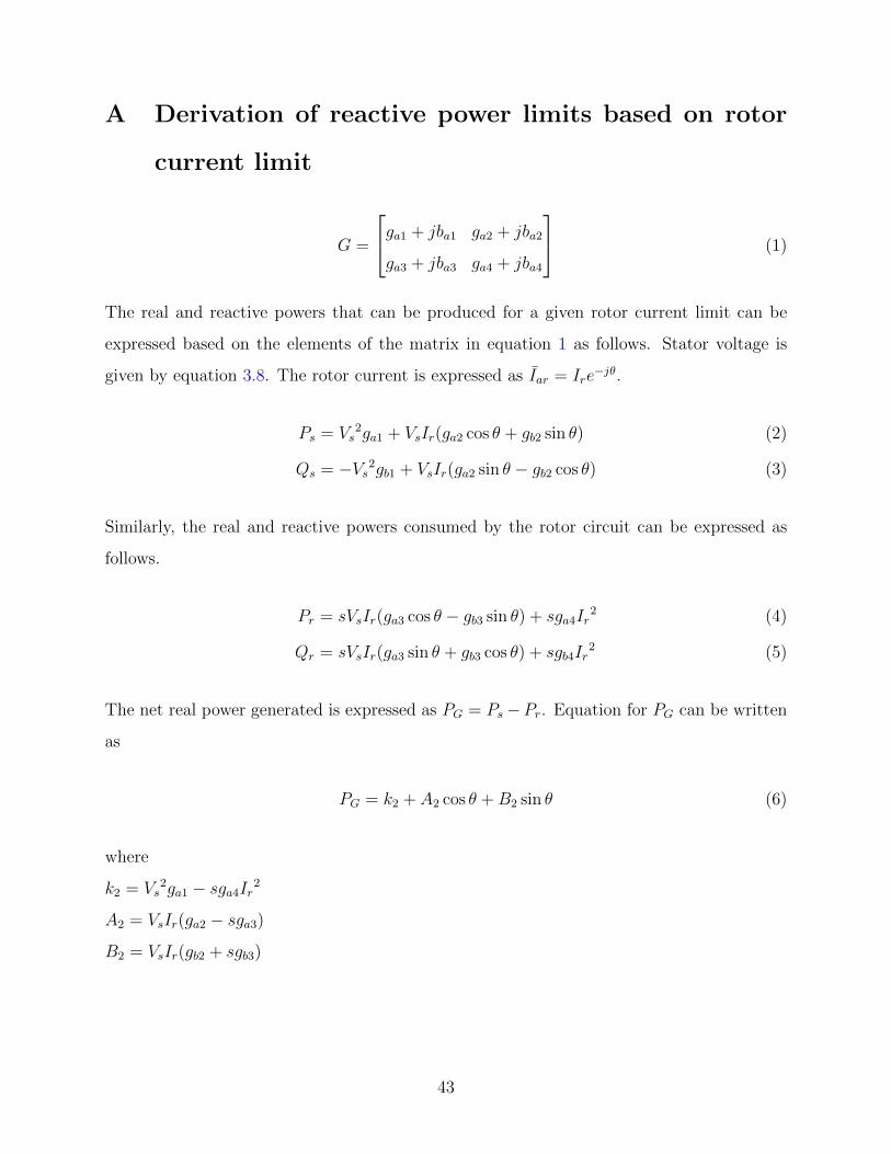
G =

ga1 + jba1 ga2 + jba2

ga3 + jba3 ga4 + jba4

(1)

The real and reactive powers that can be produced for a given rotor current limit can be

expressed based on the elements of the matrix in equation 1 as follows. Stator voltage is

given by equation 3.8. The rotor current is expressed as Iar = Ire−jθ.

Ps = Vs2ga1 + VsIr(ga2 cos θ + gb2 sin θ) (2)

Qs = −Vs2gb1 + VsIr(ga2 sin θ − gb2 cos θ) (3)

Similarly, the real and reactive powers consumed by the rotor circuit can be expressed as

follows.

Pr = sVsIr(ga3 cos θ − gb3 sin θ) + sga4Ir2 (4)

Qr = sVsIr(ga3 sin θ + gb3 cos θ) + sgb4Ir2 (5)

The net real power generated is expressed as PG = Ps−Pr. Equation for PG can be written

as

PG = k2 + A2 cos θ +B2 sin θ (6)

where

k2 = Vs2ga1 − sga4Ir

2

A2 = VsIr(ga2 − sga3)

B2 = VsIr(gb2 + sgb3)

43

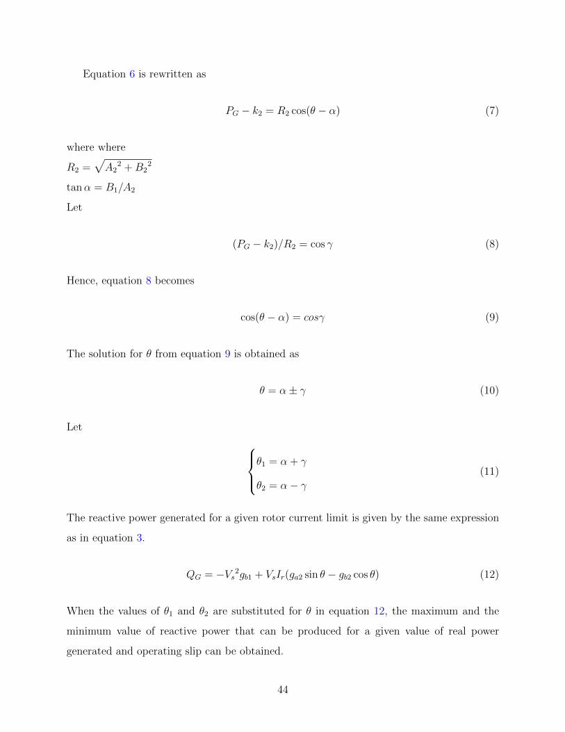
Equation 6 is rewritten as

PG − k2 = R2 cos(θ − α) (7)

where where

R2 =√A2

2 +B22

tanα = B1/A2

Let

(PG − k2)/R2 = cos γ (8)

Hence, equation 8 becomes

cos(θ − α) = cosγ (9)

The solution for θ from equation 9 is obtained as

θ = α± γ (10)

Let θ1 = α + γ

θ2 = α− γ

(11)

The reactive power generated for a given rotor current limit is given by the same expression

as in equation 3.

QG = −Vs2gb1 + VsIr(ga2 sin θ − gb2 cos θ) (12)

When the values of θ1 and θ2 are substituted for θ in equation 12, the maximum and the

minimum value of reactive power that can be produced for a given value of real power

generated and operating slip can be obtained.

44

B Derivation of reactive power limits based on stator

current limit

B =

Ba1 + jBb1 Ba2 + jBb2

Ba3 + jBb3 Ba4 + jBb4

(13)

The stator current is expressed as Ias = Isejδ. The expressions for the real and reactive

power generated for a particular stator current limit is given by the following equations.

Ps = VsIs cos δ (14)

Qs = VsIs sin δ (15)

The expressions for real and reactive power absorbed by the rotor is given below.

Pr = s(Ba1Ba3 +Bb1Bb3)Vs2 + s(Ba2Ba4 +Bb2Bb4)Is

2

+sVsIs(Ba1Ba4 +Bb1Bb4 +Ba2Ba3 +Bb2Bb3) cos δ

+sVsIs(Ba3Bb2 −Ba2Bb3 +Ba1Bb4 −Ba4Bb1) sin δ (16)

Qr = s(Ba3Bb1 −Ba1Bb3)Vs2 + s(Ba4Bb2 −Ba2Bb4)Is

2

+sVsIs(Ba4Bb1 −Ba1Bb4 +Ba3Bb2 −Ba2Bb3) cos δ

+sVsIs(Ba1Ba4 +Bb1Bb4 −Ba2Ba3 −Bb3Bb2) sin δ (17)

Net real power generated is given by PG = Ps − Pr which is obtained from expressions 14

and 16.

PG = k3 + A3 cos δ +B3 sin δ (18)

where k3 = −sVs2(Ba1Ba3 +Bb1Bb3) − sIs2(Ba2Ba4 +Bb2Bb4)

A3 = VsIs[1 − s(Ba1Ba4 +Bb1Bb4 +Ba2Ba3 +Bb2Bb3)]

45

B3 = −sVsIs[Ba3Bb2 −Ba2Bb3 −Ba4Bb1 +Ba1Bb4]

Equation 18 is rewritten as

PG − k3 = R3 cos(δ − α) (19)

where

R3 =√A3

2 +B32

tanα = B3/A3

Let PG−k3R3

= γ. Then, equation 19 is rewritten as

cos(δ − α) = cos γ (20)

Equation 20 is solved to obtain δ as

δ = α± γ (21)

Let δ1 = α + γ

δ2 = α− γ

(22)

The reactive power generated is the same as that of equation 15 and can be rewritten as

QG = VsIs sin δ (23)

Substituting the values of δ1 and δ2 for δ in equation 23, the maximum and the minimum

values of reactive power that can be generated for a given slip and real power generation is

obtained.

46

Vita

The author Jonathan Devadason has completed an undergraduate degree in electrical and

electronics engineering in the year 2008 and a master’s degree in power systems engineering in

the year 2013 from College of Engineering, Anna University, India. He is currently working

on his master’s degree in electrical engineering in the University of Tennessee, Knoxville.

His areas of interest are power system dynamics, application of power electronics in power

systems - FACTS and HVDC transmission and bifurcations in power systems.

47