Modeling and Analysis of Nanostructured Thermoelectric

Modeling and Analysis of Nanostructured Thermoelectric Power Generation and

Cooling Systems

by

Ronil Rabari

A Thesis

presented to

The University of Guelph

In partial fulfilment of requirements

for the degree of

Doctor of Philosophy

in

Engineering

Guelph, Ontario, Canada

© Ronil Rabari, October, 2015

ABSTRACT

MODELING AND ANALYSIS OF NANOSTRUCTURED THERMOELECTRIC

POWER GENERATION AND COOLING SYSTEMS

Ronil Rabari Advisors:

University of Guelph, 2015 Dr. Shohel Mahmud

Dr. Animesh Dutta

This thesis is an investigation of heat transfer processes in nanostructured thermoelectric

(TE) systems. TE systems include solid state thermoelectric generators (TEG) and thermoelectric

coolers (TEC). Current TE systems exhibit low performance (i.e., thermal efficiency and

Coefficient of Performance (COP)) compared to conventional energy conversion devices. The

higher Figure-of-Merit nanostructured TE materials can increase the performance of TE systems.

In this study, a mathematical model of a TE system was developed including the Seebeck,

Peltier, and Thomson effects, Fourier heat conduction, Joule heat, and convection heat transfer.

Numerical simulations were performed using the coupled TE constitutive equations. The

simulated results were expressed as contours of temperature and electric potential and as

streamlines of heat flow and electric current. The effective thermal conductivities, calculated

using different transport property models, were used to investigate nanostructured TE systems.

Additionally, Bismuth-Telluride based nanostructured TE materials were prepared using the

solid state synthesis method.

The study results report parameters which affect the thermal efficiency, COP, and entropy

generation in nanostructured TEG and TEC systems. These parameters include the temperature

difference, electric current, volume fraction of nanoparticles, and convection heat transfer

coefficients at different locations: the side surfaces of TE legs; between the thermal source and

the hot side of a TE system; and between the thermal sink and the cold side of a TE system. The

results show a decrease in the thermal efficiency and COP of a TEG and TEC system,

respectively, as the convection heat transfer coefficient increases. Nevertheless, a TEC system

with a higher electric potential input increases the COP with an increase in the convection heat

transfer coefficient. This study establishes that the heat conduction contribution to the total heat

input for TEG and TEC systems should remain as low as possible for maximum system

performance. The synthesized Bi2Te2.7Se0.3, using the indirect resistance heating method,

exhibited low density which may have contributed to a higher electrical resistivity and a lower

Seebeck coefficient.

The macroscopic modeling of nanostructured TE systems performed in this thesis provided

results which can be applied to the design of next generation thermal management and power

generation solutions.

iv

To all my teachers

To my loving daughters - Aarna and Archa

v

Acknowledgements

I would like to express my sincerest gratitude to Dr. Shohel Mahmud, whose expertise,

understanding, and patience has made the graduate research experience enjoyable. I appreciate

his vast knowledge and skill in different areas and his assistance in preparing research activities

and countless revisions of different parts of this work. He always goes above and beyond typical

advisor in research and advising activities. I would also like to thank co-advisor, Dr. Animesh

Dutta who was always there to listen and give advice. Next, I would like to thank committee

member, Dr. Roydon Fraser, for insightful comments and useful suggestions. I would like to

thank Dr. Sushanta Mitra for being on my Ph.D. examination committee as an external examiner.

Additionally, I would like to thank Dr. William Lubitz and Dr. Fantahun Defersha for being on

my qualifying exam committee and providing constructive feedback. The author is also thankful

to Dr. Douglas Joy, the graduate coordinator for his fruitful suggestions during the qualifying

exam. I would also like to acknowledge the help from Dr. Mohammad Biglarbegian during the

preparation of chapters 2 and 4.

The author would like to express special thanks to the Natural Sciences and Engineering

Research Council (NSERC) and the Ontario Ministry of Agriculture and Food, and Rural Affairs

(OMAFRA) for their financial support. The author is thankful to the Mitacs for the Globalink

Research Award which established new research collaboration with the Indian Institute of

Science. I am extremely thankful to Dr. Ramesh Chandra Mallik at the Department of Physics,

Indian Institute of Science, Bangalore for the technical guidance and help to prepare

nanocomposite thermoelectric materials. Additionally, the use of instruments for surface

analytical techniques and X-ray diffraction at the Indian Institute of Science is very much

appreciated. I would also like to also thank the thermoelectric research group at the Indian

Institute of Science: Dr. Raju Chetty, Dr. Ashoka Bali, Prem Kumar, Sayan Das, and Nilanchal

Patra for their help and technical discussions.

The author would like to thank Mike Speagle for his help in laboratory activities. I would

also like to thank Joel Best, John Whiteside, Ryan Smith, Ken Graham, Nathaniel Groendyk,

Hong Ma, Phil Watson, and David Wright for their help during various stages of this research. I

would also like to thank Laurie Gallinger, Paula Newton, Izabella Onik, Martha Davies, and

Paige Clark for their administrative help. I warmly acknowledge the cooperation and fruitful

vi

discussions with research group at the Advanced Energy Conversion and Control Lab,

University of Guelph: Muath Alomair, Yazeed Alomair, Shariful Islam, Manar Al-Jethelah,

Kaswar Jamil, Rakib Hossain, and Raihan Siddique. Author is also thankful to Tijo Joseph,

Mohammad Tushar, Bimal Acharya, Dr. Poritosh Roy, Jamie Minaret, and Harpreet Kambo at

the University of Guelph and Vaibhav Patel at the Indian Institute of Science for their generous

help.

I am extremely grateful to my parents and grandparents for the unconditional support they

provided during this journey. I must acknowledge encouragement, help, and love from my wife,

Unnati, without her I would not have finished this thesis.

vii

Table of Contents

Cover page i

Abstract ii

Dedication iv

Acknowledgements v

Table of contents vii

List of figures ix

List of tables xix

Chapter 1 Introduction 1

1.1 Background 1

1.2 Objectives 5

1.3 Scope of this thesis 7

1.4 Contribution of present study 11

1.5 Publications from present study 12

Chapter 2 Effect of convection heat transfer on performance of waste heat

thermoelectric generator 13

2.1 Introduction 13

2.2 Heat transfer modeling 16

2.3 Results and discussion 21

2.4 Conclusion 53

2.5 Nomenclature 54

Chapter 3 Numerical simulation of nanostructured thermoelectric generator

considering surface to surrounding convection 56

3.1 Introduction 56

3.2 Mathematical model and boundary conditions 60


3.4 Conclusion 76

3.5 Nomenclature 77

Chapter 4 Analytical and numerical studies of heat transfer in nanocomposite

thermoelectric cooler 79

viii

4.1 Introduction 79

4.2 Modeling 81


4.4 Conclusions 135

4.5 Nomenclature 136

Chapter 5 Effect of thermal conductivity on performance of thermoelectric systems

based on effective medium theory 138

5.1 Introduction 138

5.2 Modeling and boundary conditions 144


5.4 Conclusion 199


Chapter 6 Analysis of combined solar photovoltaic-nanostructured thermoelectric

generator system 202


6.2 Modeling and boundary conditions 205

6.3 Results 213

6.4 Conclusion 235


Chapter 7 Nanostructuring of n-type Bi2Te2.7Se0.3 based on solid state synthesis

technique 239


7.2 Sample preparation and results 241

7.3 Conclusion 248

Chapter 8 Overall conclusions and future work 249

8.1 Overall conclusions 249

8.2 Future work 250

References 251

ix

List of Figures

Figure

number

Title Page

number

1.1 Typical TE modules in power generation mode or cooling mode 3

1.2 Potential applications of TE systems (Pichanusakorn and Bandaru

2010)

4

2.1 Various waste heat recovery methods in context of power plant

(Stehlik 2007, Rowe 1995)

13

2.2 Schematic diagram of location of TEG in combustion system and the

schematic view of unit TEG cell

17

2.3 Temperature distribution over the length of p-type semiconductor leg

with thermal source temperature, HT 700 K and thermal sink

temperature, CT 300 K

24

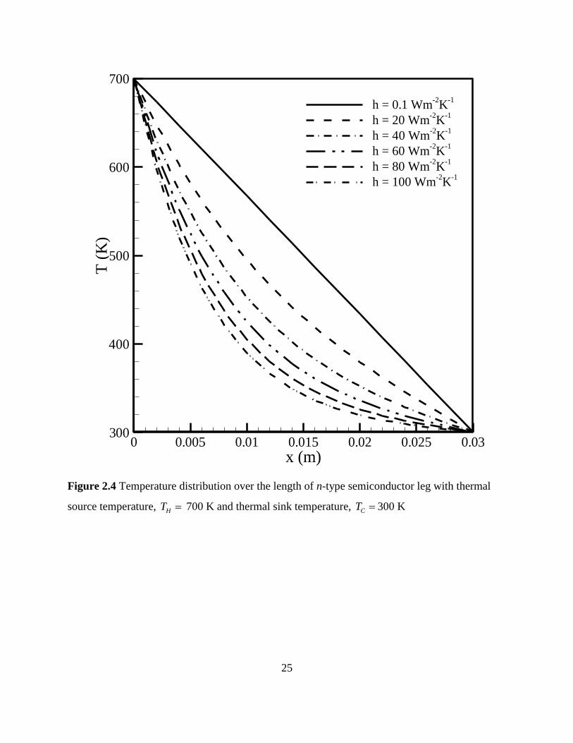
2.4 Temperature distribution over the length of n-type semiconductor leg

with thermal source temperature, HT 700 K and thermal sink


25

2.5 Effect of thermal source temperature on heat input with variable

convection heat transfer coefficient at constant thermal sink


27

2.6 Effect of thermal sink temperature on heat input with variable

convection heat transfer coefficient at constant thermal source

temperature, HT 700 K

28

2.7 Power generation as a function of thermal source temperature at

different thermal sink temperature

30

2.8 Effect of thermal source temperature on thermal efficiency with

variable convection heat transfer coefficient at constant thermal sink


32

2.9 Effect of thermal sink temperature on thermal efficiency with variable 33

x

convection heat transfer coefficient at constant thermal source

temperature, HT 700 K

2.10 Current as a function of thermal source temperature with different

thermal sink temperature

34

2.11 Effect of convection heat transfer coefficient on thermal efficiency at

constant thermal sink temperature, CT 300 K

36

2.12 Effect of convections between the thermal source and the top surface

and between the sink and the bottom surface of TEG on thermal

efficiency when HT 700 K and CT 300 K with adiabatic side wall

condition

37

2.13 Effect of convections between the thermal source and the top surface

and between the sink and the bottom surface of TEG on thermal

efficiency when HT 700 K and CT 300 K with convection from the

side walls with h 10 Wm-2

K-1

38

2.14 Entropy generation rate as a function of thermal source temperature at

different convection heat transfer coefficients with constant thermal

sink temperature, CT 300 K

42

2.15 Temperature distribution in TEG with adiabatic boundary conditions at

vertical walls of semiconductor legs

45

2.16 Electrical potential in TEG with adiabatic boundary conditions at


46

2.17 Temperature distribution in TEG with convective boundary conditions,

h = 20 Wm-2

K-1

at vertical walls semiconductor legs

47

2.18 Electrical potential in TEG with convective boundary conditions, h =

20 Wm-2

K-1

at vertical walls of semiconductor legs

48

2.19 Comparison of heat input, power output, and thermal efficiency

obtained from the current work with the similar results available in

(Angrist 1982)

51

2.20 Comparison of analytical and numerical results in terms of temperature 52

xi

distribution over the p-type semiconductor leg

3.1 Schematic of unit cell of TEG 60

3.2 Contours of temperature distribution and streamlines of heat flow with

adiabatic heat transfer condition (h ≈ 0 W/m2K)

65

3.3 Contours of electric potential and streamlines of electric current flow

with adiabatic heat transfer condition (h ≈ 0 W/m2K)

66


adiabatic heat transfer condition (h = 15 W/m2K)

67


with adiabatic heat transfer condition (h = 15 W/m2K)

68



69



70



71



72

3.10 Comparison of current production using numerical and analytical

techniques

74

3.11 Thermal efficiency of TEG as a function of convection heat transfer

coefficient and temperature difference

75

4.1 Schematic diagram of unit cell of TEC (drawing is not to scale) 82

4.2 The schematic of crystal structure of (a) (Bi1-xSbx)2Te3 (Zhang et al.

2011) Reprinted by permission from Macmillan Publishers Ltd: Nature

Communications from Zhang et al.2, 574 (2011), copyright 2011

83

4.3 The schematic of crystal structure of Bi2Te3 (Chen et al. 2009) From

[Chen et al. Science 325, 178 (2009)]. Reprinted with permission from

AAAS

84

4.4 Temperature distribution over the length of p-type TE leg with hot 89

http://www.nature.com/ncomms/journal/v2/n12/abs/ncomms1588.html


http://www.sciencemag.org/content/325/5937/178



xii

surface temperature 353 K and cold surface temperature 333 K

4.5 Temperature distribution over the length of n-type TE leg with hot

surface temperature 353 K and cold surface temperature 333 K 90

4.6 Electrical resistivity of p- and n- type legs of nanocomposite TEC 91

4.7 Heat absorbed as a function of current considering hot surface

temperature 353 K with cold surface temperature 333 K

93

4.8 Heat absorbed as a function of current considering hot surface


94

4.9 COP of TEC as a function of current considering hot surface


96

4.10 COP of TEC as a function of current considering hot surface


97

4.11 Heat absorbed as a function of temperature difference with different

electric current input and hot surface temperature 353 K considering

adiabatic side wall condition

99

4.12 COP as a function of temperature difference with different electric

current input and hot surface temperature 353 K considering adiabatic

side wall condition

100

4.13 Maximum heat absorbed of TEC considering variable convection heat

transfer coefficient and variable TE leg heights with hot surface

temperature 353 K and cold surface temperature 333 K

101

4.14 Optimum electric current for maximum heat absorption of TEC

considering variable convection heat transfer coefficient and variable

TE leg heights with hot surface temperature 353 K and cold surface

temperature 333 K

104

4.15 Maximum COP of TEC considering variable convection heat transfer

coefficient and variable TE leg heights with hot surface temperature

353 K and cold surface temperature 333 K

105

4.16 Optimum electric current for maximum COP of TEC considering

variable convection heat transfer coefficient and variable TE leg

106

xiii

heights with hot surface temperature 353 K and cold surface

temperature 333 K

4.17 Internal resistance of TEC unit cell as a function of TE leg height 108

4.18 Maximum heat absorbed as a function of TE leg height by unit cell of

TEC with hot surface temperature 353 K, cold surface temperature 333

K, and adiabatic side wall condition

109

4.19 Electric scalar potential and current flow in nanocomposite TEC with

electric potential 0.02 V

111

4.20 Electric scalar potential and current flow in nanocomposite TEC with


112

4.21 Heat flow and temperature distribution in nanocomposite TEC for h ≈

0 Wm-2

K-1

at vertical walls with electric potential 0.02 V

114

4.22 Heat flow and temperature distribution in nanocomposite TEC for h =

20 Wm-2

K-1


115


40 Wm-2

K-1


116


60 Wm-2

K-1


117

4.25 Heat flow and temperature distribution in nanocomposite TEC for h ≈

0 Wm-2

K-1


119


60 Wm-2

K-1


120

4.27 Heat absorbed by nanocomposite TEC as a function of convection heat

transfer coefficient with hot surface temperature 353 K and electric

potential 0.02 V

121

4.28 COP of nanocomposite TEC as a function of convection heat transfer

coefficient with hot surface temperature 353 K and electric potential

0.02 V

123

4.29 Heat absorbed by nanocomposite TEC as a function of convection heat

transfer coefficient with hot surface temperature 353 K and electric

125

xiv

potential 0.06 V

4.30 COP of nanocomposite TEC as a function of convection heat transfer

coefficient with hot surface temperature 353 K and electric potential

0.06 V

126

4.31 Comparison of analytical and numerical simulation results in terms of

heat absorbed considering variable convection heat transfer coefficient

with hot surface temperature 353 K, cold surface temperature 333 K,

and electric potential 0.02 V

128

4.32 Comparison of analytical and numerical simulation results in terms of

COP considering variable convection heat transfer coefficient with hot

surface temperature 353 K, cold surface temperature 333 K, and


129

4.33 Comparison of COP using conventional (no nanostructuring) and

nanocomposite TE material considering h ≈ 0 Wm-2

K-1

, hot surface

temperature 353 K, and electric current input of 1 A

131

4.34 Thermal conductivity of conventional (no nanostructuring) and

nanocomposite TE materials

132

4.35 Comparison of results between current work and Poudel et al. (2008) 134

5.1 Different approaches to increase ZT of TE materials (Martin-Gonzalez

2013)

139

5.2 Graphical representation of (a) Maxwell model (b) Hasselman and

Johnson model (c) Minnich and Chen model

142

5.3 Schematic diagram of typical (a) TEC and (b) TEG system 144

5.4 Effective thermal conductivity of p-type and n-type thermoelectric

material based on Maxwell model

150

5.5 Effective thermal conductivity of p-type and n-type thermoelectric

material based on Hasselman-Johnson model

152

5.6 Effect of thermal boundary conductance on effective thermal

conductivity of p-type using Hasselman-Johnson model

154

5.7 Effect of thermal boundary conductance on effective thermal 155

xv

conductivity of n-type using Hasselman-Johnson model

5.8 Effective thermal conductivity of p-type thermoelectric material using

Minnich-Chen model

157

5.9 Effective thermal conductivity of n-type thermoelectric material using

Minnich-Chen model

158

5.10 COP of TEC considering various amount of volume fraction with

Maxwell model

161

5.11 Efficiency of TEG with different volume fraction with Maxwell model 162

5.12 COP of TEC considering different amount of volume fraction with

Hasselman model

164

5.13 Efficiency of TEG with different amount of volume fraction with

Hasselman model

165

5.14 Effect of boundary conductance on performance of TEC based on

Hasselman-Johnson model

166

5.15 Effect of boundary conductance on performance of TEG based on


167

5.16 COP of TEC considering different amount of volume fraction with

Minnich-Chen model

169

5.17 Efficiency of TEG with different volume fraction with Minnich-Chen

model

170

5.18 Effect of nanoparticle size on performance of TEC considering

Minnich-Chen model

171

5.19 Effect of nanoparticle size on performance of TEG considering

Minnich-Chen model

172

5.20 Performance of TEC with variable volume fractions and convection

heat transfer coefficients through side walls of TE legs

174

5.21 Performance of TEG with variable volume fractions and convection

heat transfer coefficients through side walls of TE legs

175

5.22 Influence of effective thermal conductivity on heat conduction in TEC 177

5.23 Influence of effective thermal conductivity on heat conduction in TEG 178

xvi


in TEC

180

5.25 Contours of temperature and streamlines of heat flow in TEC with cold

surface temperature 290 K, hot surface temperature 300 K, and electric

potential 0.02 V with NO particles

182



potential 0.02 V with 0.8 volume fraction with Maxwell model

183



potential 0.02 V with 0.8 volume fraction with Hasselman-Johnson

model

184



potential 0.02 V with 0.8 volume fraction with Minnich-Chen model

185

5.29 Contours of temperature and streamlines of heat flow in TEG with cold

surface temperature 300 K and hot surface temperature 350 K with NO

particles

187


surface temperature 300 K and hot surface temperature 350 K with 0.8

volume fraction with Maxwell model

188



volume fraction Hasselman-Johnson model

189



volume fraction with Minnich-Chen model

190

5.33 Contours of electric potential and streamlines of electric current in

TEG with cold surface temperature 300 K and hot surface temperature

350 K with NO particles

192

xvii



350 K with 0.8 volume fraction with Maxwell model

193



350 K with 0.8 volume fraction Hasselman-Johnson model

194



350 K with 0.8 volume fraction with Minnich-Chen model

195

5.37 Comparison of analytical and numerical simulation results for TEC 197

5.38 Comparison of analytical and numerical simulation results for TEG 198

6.1 Schematic diagram of (a) photovoltaic – thermoelectric (PVTE)

system and (b) unit thermoelectric generator

207

6.2 Exploded view of Solar PV panel layers (Amrani 2007) 207

6.3 Solar PV panel back surface temperature with variable solar radiation

and ambient temperature

218

6.4 Temperature distribution over the length of nanostructured p type

and n type semiconductor leg

219

6.5 Heat input to nanostructured TE generator with different solar radiation

and variable convection heat transfer coefficient

222

6.6 Heat input comparison of TE generator using traditional and

nanostructured material thermoelectric material

223

6.7 Thermal conductivity of traditional and nanostructured TE material as

a function of temperature

224

6.8 Power output from TE generator as a function of solar radiation 226

6.9 Thermal efficiency of nanostructured TE generator with different solar

radiation and variable convection heat transfer coefficient

228

6.10 Thermal efficiency comparison of TE generator with traditional and

nanostructured TE material 229

xviii

6.11 Power output comparison of solar PV panel and TE generator 231

6.12 Solar panel conversion efficiency Vs. Solar Radiation 233

6.13 Combined efficiency of solar PVTE system Vs. Solar Radiation 234

7.1 ZT improvements in low dimensional and bulk TE materials 240

7.2 Rietveld refinement power XRD pattern for Bi2Te2.7Se0.3 242

7.3 Seebeck coefficient and Electrical resistivity of sample Bi2Te2.7Se0.3 243

7.4 Power factor of sample Bi2Te2.7Se0.3 244

7.5 Comparison of power factor between Bi2Te2.7Se0.3 manufactured via

direct current hot press and indirect resistance heating

246

7.6 SEM image of fractured surfaces of hot pressed sample 247

xix

List of Tables

Table

number

Title Page

number

1.1 Comparison of various waste heat recovery methods (BCS 2008) 2

1.2 Contribution of present study 11

2.1 Temperature dependent TE properties of n-type 75% Bi2Te3 25%

Bi2Se3 and p-type 25% Bi2Te375% Sb2Te3 with 1.75% excess Se

(Reddy et al. 2013, Angrist 1982)

22

2.2 Thermal efficiency of single unit of TEG with cold surface

temperature, CT = 300 K

50

3.1 Polynomial functions of Seebeck coefficient, electrical conductivity,

and thermal conductivity as a function of temperature for BiSbTe

nanostructured bulk alloys and Bi2Te3 with SiC nanoparticles (Poudel

et al. 2008, Zhao et al. 2008)

63


and thermal conductivity as a function of temperature for BiSbTe

nanostructured bulk alloys and nanocomposite Bi2Te3 (Poudel et al.

2008, Fan et al. 2011)

87


and thermal conductivity as a function of temperature for BiSbTe bulk

alloys and conventional Bi2Te3 (Poudel et al. 2008, Fan et al. 2011)

87

4.3 Height of TE legs and internal resistance of TEC for different cases

considered in Figs. 4.13, 4.14, 4.15, and 4.16

101

5.1 Comparison of different effective medium theories 143

5.2 Material properties (Pattamatta and Madnia 2009) 149

6.1 Operating conditions and dimensional parameters of combined solar

PVTE system

214


thermal conductivity, and figure of merit with respect to temperature

for nanostructured BiSbTe bulk alloys (Poudel et al. 2008)

215

xx


thermal conductivity, and figure of merit with respect to temperature

for BiSbTe bulk alloys (Poudel et al. 2008)

216

1

CHAPTER 1: INTRODUCTION

1.1 Background

Forty percent of the world’s energy demand is met by energy conversion systems (e.g., coal

power stations) which convert low-grade energy (e.g., coal) into high-grade energy (e.g.,

electricity) (Zhang et al. 2010). Most of the energy conversion systems produce waste heat

which leads to a lower efficiency of the overall energy conversion process. For example, 60% of

the energy from a power station is lost as a waste heat (EEA 2008). In a similar manner, internal

combustion engines which are used in most of the current transport vehicles waste 60-70% of the

input energy (Nolas et al. 2006; Bottner et al. 2006). The U.S. Department of Energy (DOE

2011) considers increment in the efficiency of energy conversion systems as one of the strategies

to address the energy demand. Waste heat recovery is one of the methods to increase the

efficiency of energy conversion systems which in turns answers the energy challenge.

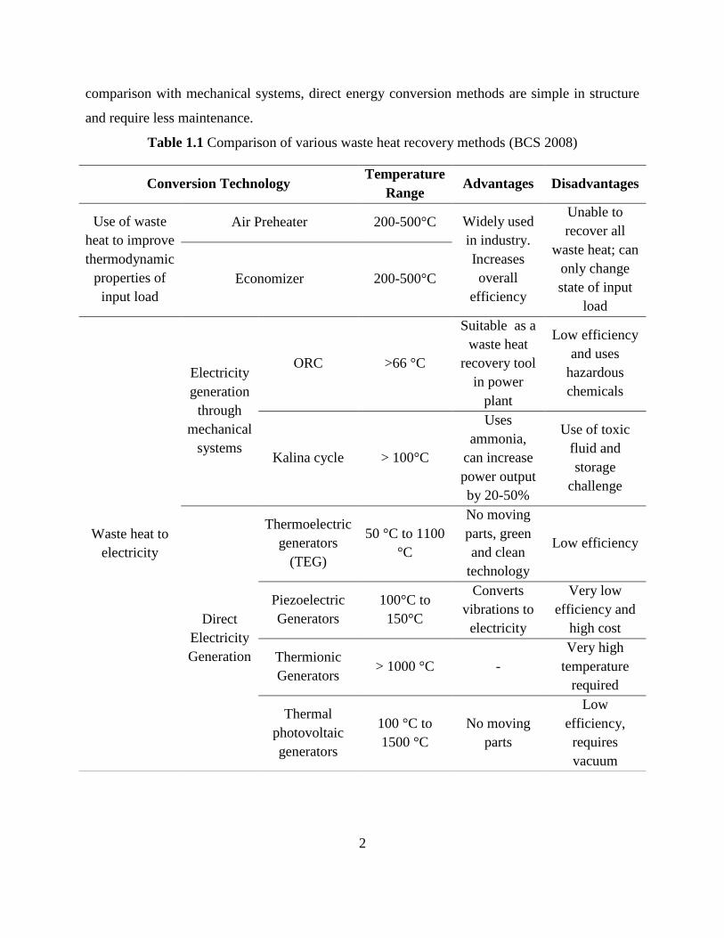
Waste heat recovery solutions can be applied in different ways depending upon the applications

(BCS 2008). Table 1.1 shows different waste heat recovery solutions in terms of temperature

ranges, advantages, and disadvantages. Waste heat recovery solutions can be broadly classified

into two categories; temperature increment of input fluid and electricity generation. Further,

electricity generation can be classified into two categories: using mechanical systems (i.e.,

moving parts) and direct electricity generation (i.e., without moving parts). An industrial or

power station operation applies an air preheater and economizer to improve the temperature of

the input fluid. Some industries utilize modified versions of the basic Rankine cycle such as the

Organic Rankine Cycle (ORC) and Kalina cycle to generate electricity. The Organic Rankine

Cycle (ORC) and the Kalina cycle use fluids with low boiling temperatures such as propane, iso-

pentane, toluene, and ammonia (BCS 2008). The ORC and Kalina cycle, which use hazardous

chemicals, suffer from low efficiency, and requires continuous maintenance due to rotating parts.

On the other hand, direct electricity generation methods convert thermal energy to electricity

without using any harmful chemicals and moving parts. Some of the techniques include

piezoelectric, thermal-photovoltaic, thermionic, and thermoelectric energy conversion. In

2

comparison with mechanical systems, direct energy conversion methods are simple in structure

and require less maintenance.

Table 1.1 Comparison of various waste heat recovery methods (BCS 2008)

Conversion Technology Temperature

Range Advantages Disadvantages

Use of waste

heat to improve

thermodynamic

properties of

input load

Air Preheater 200-500°C Widely used

in industry.

Increases

overall

efficiency

Unable to

recover all

waste heat; can

only change

state of input

load

Economizer 200-500°C

Waste heat to

electricity

Electricity

generation

through

mechanical

systems

ORC >66 °C

Suitable as a

waste heat

recovery tool

in power

plant

Low efficiency

and uses

hazardous

chemicals

Kalina cycle > 100°C

Uses

ammonia,

can increase

power output

by 20-50%

Use of toxic

fluid and

storage

challenge

Direct

Electricity

Generation

Thermoelectric

generators

(TEG)

50 °C to 1100

°C

No moving

parts, green

and clean

technology

Low efficiency

Piezoelectric

Generators

100°C to

150°C

Converts

vibrations to

electricity

Very low

efficiency and

high cost

Thermionic

Generators > 1000 °C -

Very high

temperature

required

Thermal

photovoltaic

generators

100 °C to

1500 °C

No moving

parts

Low

efficiency,

requires

vacuum

3

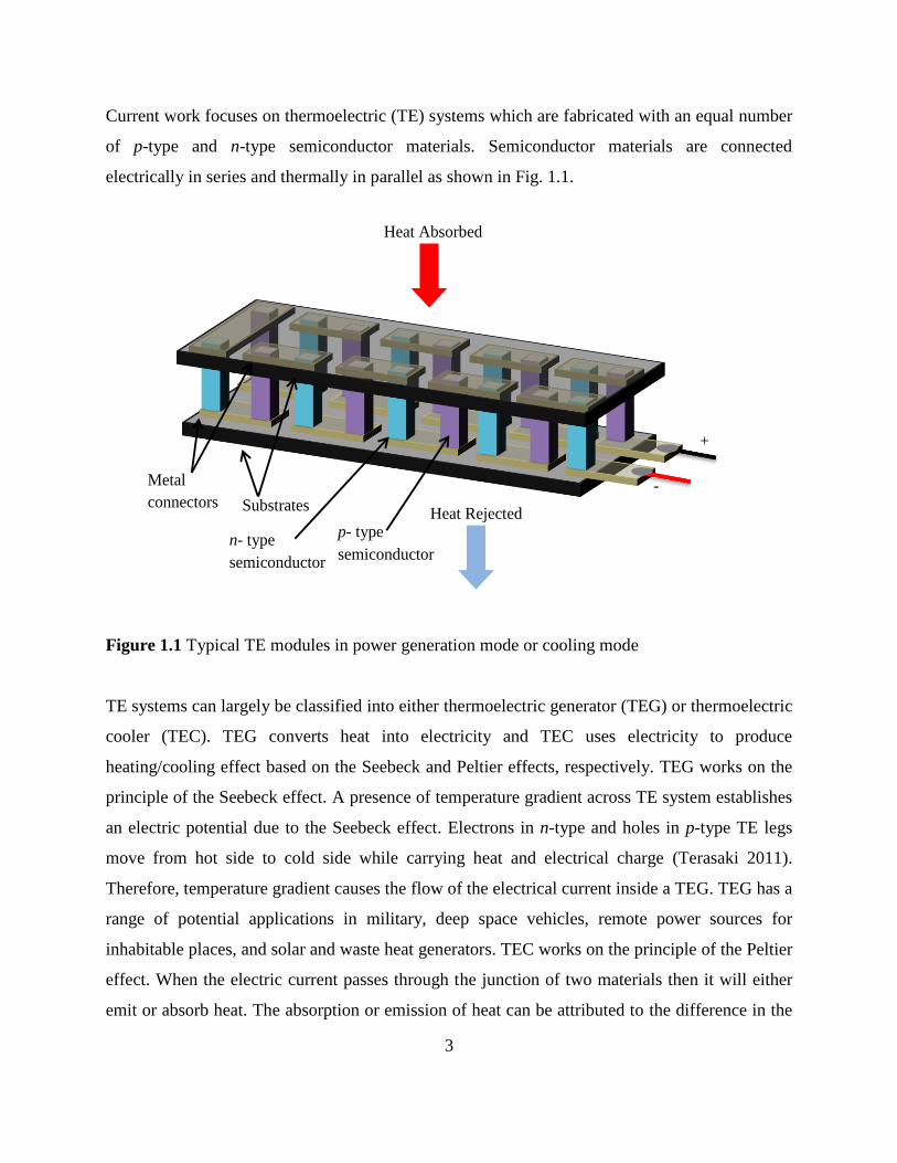
Current work focuses on thermoelectric (TE) systems which are fabricated with an equal number

of p-type and n-type semiconductor materials. Semiconductor materials are connected

electrically in series and thermally in parallel as shown in Fig. 1.1.

Figure 1.1 Typical TE modules in power generation mode or cooling mode

TE systems can largely be classified into either thermoelectric generator (TEG) or thermoelectric

cooler (TEC). TEG converts heat into electricity and TEC uses electricity to produce

heating/cooling effect based on the Seebeck and Peltier effects, respectively. TEG works on the

principle of the Seebeck effect. A presence of temperature gradient across TE system establishes

an electric potential due to the Seebeck effect. Electrons in n-type and holes in p-type TE legs

move from hot side to cold side while carrying heat and electrical charge (Terasaki 2011).

Therefore, temperature gradient causes the flow of the electrical current inside a TEG. TEG has a

range of potential applications in military, deep space vehicles, remote power sources for

inhabitable places, and solar and waste heat generators. TEC works on the principle of the Peltier

effect. When the electric current passes through the junction of two materials then it will either

emit or absorb heat. The absorption or emission of heat can be attributed to the difference in the

Heat Rejected Substrates

Metal

connectors

p- type

semiconductor

-

+

n- type

semiconductor

Heat Absorbed

4

chemical potential of the two materials (Terasaki 2011). TEC also has a wide range of potential

applications in electronics, laser diodes, military garments, laboratory cold plates, and

transportation systems. Figure 1.2 illustrates a brief glimpse of potential applications of TE

systems in terms of power usage and generation. TE systems have many advantages such as

simple structure, no moving parts, and quiet in operation (Silva and Kaviany 2004). Moreover,

they have no adverse effect on the environment and have a long service life. TE systems can

easily work in tandem with conventional technologies under a wide temperature range which

makes them an ideal candidate for the waste heat recovery. However, because of their low

conversion efficiency, current TE systems have limited applications (Gonzalez et al. 2013).

Figure 1.2 Potential applications of TE systems (Pichanusakorn and Bandaru 2010)

In order to better understand TE systems, the coupled effects of heat transfer and electric

potential need to be understood. In most of the work, a heat transfer model does not account for

all internal and external heat transfer irreversibilities. It is well established that irreversibilities in

100 W

10 W

1 W

100 mW

10 mW

1 mW

100 µW

10 µW

1 µW

1 kW

Power 10 kW

Low power applications; wrist-watches

Biomedical devices; pacemakers

Remote wireless sensors

Deep space vehicles power and cooling

Consumer refrigerators, electronic cooling

Waste heat recovery; (e.g., powerstation, automotive,

redundant oil wells and nuclear facility)

5

energy conversion systems can increase the entropy and lead to the destruction of the exergy

(Bermejo 2013). In addition to this, TE systems suffer from low conversion efficiency due to the

poor material properties. Recent advancements in nanostructuring of TE materials have enhanced

the material properties and improved the conversion efficiency (Ma et al. 2013). One of the ways

to improve the TE properties is to lower the thermal conductivity (Bhandari 1995). A low-

dimensional (e.g., 0D, 1D, 2D) nanostructured TE material with the lower thermal conductivity

is costly to manufacture and difficult to apply in real world applications. However, a new set of

TE bulk nanostructured materials called “nanocomposites” offer an alternative to low-

dimensional TE structures. Therefore, the present research aims to study heat transfer in

nanocomposite TEG and TEC. The work develops mathematical models and numerical

simulations to study the heat transfer in nanocomposite TE systems. This study provides

parameters (e.g., temperature difference, convection heat transfer coefficient, electric current,

volume fraction of nanoparticles) affecting the performance of nanocomposite TE systems (e.g.,

thermal efficiency, Coefficient of Performance (COP)). This work also shows the effects of

combining TE systems with conventional energy conversion systems. Further, experimental

work also shows how critical parameters (e.g., temperature, pressure, heating method) affect the

properties of nanocomposite TE legs.

1.2 Objectives

The overall objective of this research is to develop heat transfer models of nanostructured TE

systems. The performance of nanostructured TE systems will be evaluated both quantitatively

and qualitatively through a 1D analytical model and a 2D numerical analysis, respectively. In

addition to this, a nanostructured TE system will be combined with conventional energy

conversion systems (solar panel) and the performance will be quantified using both

nanostructured and non-nanostructured TE materials. Furthermore, nanostructured TE materials

will be developed by the solid-state synthesis technique.

The specific objectives include:

Modeling and analysis of the heat transfer and irreversibility in TEG systems with

temperature dependent material properties.

6

o Developing a heat transfer model including the Seebeck, Peltier, and Thomson effects,

Joule heating, Fourier heat conduction, and convection heat losses through side walls of

the TE legs.

o Studying entropy generation within the TEG.

o Studying effects of heat transfer on thermal efficiency and power output of TEG.

Modeling and analysis of the heat transfer and irreversibility of TEG numerically with

temperature dependent TE properties with non-nanostructured and nanostructured materials.

o Identify the effects of internal irreversibilities on the performance of non-nanostructured

and nanostructured TE system.

Modeling and analysis of the heat transfer and irreversibilities in a nanocomposite TEC

o Developing heat transfer model including the Seebeck, Peltier, and Thomson effects,

Joule heating, Fourier heat conduction, and convection heat transfer from side walls of

TE legs in TEC

o Studying effects of convection heat transfer on the performance of TEC (COP, heat

absorbed, and optimum electric current) with temperature dependent properties

o Numerical simulations of TEC with variable convection heat transfer coefficient from

side surfaces of TE legs

Investigation of nanocomposite TE system using effective thermal conductivity based on

Effective Medium Theory (EMT)

o Investigating nanoparticles’ effect on the thermal conductivity of TE nanocomposite

materials; effects of volume fraction, size and shape of nanoparticles, and thermal

conductivities of nanoparticles and base material.

o Investigating nanoparticles’ effects on the heat transfer, thermal efficiency, and COP of

TE nanocomposite systems.

Investigation of TEG in combination with conventional energy conversion system

o Identifying performance curves of TE system using non-nanostructured and

nanostructured TE materials.

o Investigating the performance of combined energy conversion system based on common

input parameters such as energy input and temperature.

Nanostructuring of n-type Bi2Te2.7Se0.3 based on solid state synthesis technique

7

o Fabricating Bismuth-Telluride based TE legs using the indirect resistance heating method

o Measuring Seebeck coefficient and electrical resistivity of nanocomposite TE leg

1.3 Scope of this thesis

The work is divided around overall objective but separated into several chapters which can stand

on its own. Due to different system considerations, the nomenclature is different for each

chapter. The research comprises six chapters, scopes of which are explained in this section.

Chapter 2: Effect of convection heat transfer on performance of waste heat thermoelectric

generator

Efficiency of energy conversion processes can be improved if waste heat is converted to

electricity. A TEG can directly convert waste heat to electricity. The TEG typically suffers from

low efficiency due to various reasons, such as ohmic heating, surface-to-surrounding convection

losses, and unfavorable material properties. In this work, the effect of surface-to-surrounding

convection heat transfer losses on the performance of TEG is studied analytically and

numerically. A one-dimensional (1-D) analytical model is developed that includes surface

convection, conduction, ohmic heating, Peltier, Seebeck, and Thomson effects with top and

bottom surfaces of TEG exposed to convective boundary conditions. Using the analytical

solutions, different performance parameters (e.g., heat input, power output, and efficiency) are

calculated and expressed graphically as functions of thermal source and sink temperatures and

convection heat transfer coefficient. Finally, a two-dimensional (2-D) mathematical model is

solved numerically to observe qualitative results of thermal and electric fields inside the TEG.

For all calculations, temperature dependent thermal/electric properties are considered. Increase in

thermal source temperature results in an increase in the power output with adiabatic side wall

conditions. A change in boundary condition to convection heat transfer from adiabatic boundary

has a large impact on thermal efficiency.

Chapter 3: Numerical simulation of nanostructured thermoelectric generator considering

surface to surrounding convection

8

TE systems can directly convert heat to electricity and vice-versa by using semiconductor

materials. Therefore, coupling between heat transfer and electric field potential is important to

predict the performance of TEG systems. This work develops a general two-dimensional

numerical model of a TEG system using nanostructured TE semiconductor materials. A TEG

with p-type nanostructured material of Bismuth Antimony Telluride (BiSbTe) and n-type

Bismuth Telluride (Bi2Te3) with 0.1 vol% Silicon Carbide (SiC) nanoparticles is considered for

performance evaluations. Coupled TE equations with temperature dependent transport properties

are used after incorporating Fourier heat conduction, Joule heating, Seebeck effect, Peltier effect,

and Thomson effect. The effects of temperature difference between the hot and cold junctions

and surface to surrounding convection on different output parameters (e.g., thermal and electric

fields, power generation, thermal efficiency, and current) are studied. Selected results obtained

from current numerical analysis are compared with the results obtained from the analytical

model available in the literature. There is a good agreement between the numerical and analytical

results. The numerical results show that as temperature difference increases output power and

amount of current generated increases. Moreover, it is quite apparent that convective boundary

condition deteriorates the performance of TEG.

Chapter 4: Analytical and numerical studies of heat transfer in nanocomposite

thermoelectric cooler

TEC can produce a cooling effect (in refrigerator mode) or a heating effect (in heat pump mode)

using electrical energy input. Performance characteristics of typical TECs are poor when

compared to the traditional cooling system (e.g., vapor compression system). However,

nanostructuring of TE materials can generate high-performance TE materials (e.g., high Seebeck

coefficient, low thermal conductivity, and high electrical conductivity), and such materials show

the promise to improve the performance of TEC. The main objective of this work is to

investigate the effect of nanocomposite TE materials and surface to surrounding convection heat

transfer on the thermal performance of TEC. The mathematical model developed in this work

includes Fourier heat conduction, Joule heat, Seebeck effect, Peltier effect, and Thomson effect.

This model also includes temperature dependent transport properties. Governing transport

equations are solved numerically using the finite element method to identify the temperature and

9

electrical potential distributions and to calculate heat absorbed and the COP. Heat absorbed and

COP are also calculated using a simplified 1D analytical solution and compared with

numerically obtained results. An optimum electric current is also calculated for maximum heat

absorption rate and maximum COP for fixed geometric dimensions and variable convection heat

transfer coefficients. An increase in the convection heat transfer coefficient increases the

optimum electric current required for maximum heat absorption rate and maximum COP. For the

materials considered, results show that COP of TEC can be increased approximately by 13% ±

1% if nanostructured TE materials are used instead of the conventional TE materials.

Chapter 5: Effect of thermal conductivity on performance of thermoelectric systems based

on effective medium theory

Currently, TE systems have very low efficiency due to unfavorable TE properties (e.g., high

thermal conductivity and low power factor). Figure of Merit is a measure of TE material’s

performance which suggests that relatively lower thermal conductivity of TE materials can

improve the performance (e.g., efficiency and coefficient of performance) of TE systems. A bulk

composite TE material made-up of TE micro or nanoparticles and base TE materials can have

low thermal conductivity. There are various models reported in the literature based on the EMT

which can predict the thermal conductivity of composites. In this work, three different models

based on the EMT are applied to investigate the performance of TEG and TEC. These models

are Maxwell model, Hasselman - Johnson model, and Minnich - Chen model. Analytical

modeling and numerical simulations have been performed to evaluate the performance (e.g.,

COP and thermal efficiency) of TE systems. Thermal efficiency of TEG increases from 2.06% to

5.59%, which is 170% rise when thermal conductivity of composite decreases from 1.1 Wm-1

K-1

to 0.11 Wm-1

K-1

based on the Minnich – Chen model with a particle size of 100 nm. An increase

in the thermal efficiency or COP can be attributed to a reduction in Fourier heat conduction

contribution to total heat input which leads to increase in total heat input. Results also show that

the performance of TE systems significantly depends on the size and volume fraction of

particles.

10

Chapter 6: Analysis of combined solar photovoltaic-nanostructured thermoelectric

generator system

In this work, a combined solar photovoltaic and TE generator system is investigated. A TE

generator converts the temperature gradient into electricity that improves the overall

performance of the combined system. A nanostructured BiSbTe TE material is used in this

investigation and its power generation performance is compared with non-nanostructured

BiSbTe TE material. Using analytical solutions, different performance parameters (e.g. heat

input, power output, efficiency) are calculated and expressed graphically as a function of solar

radiation and convection heat transfer coefficient. In addition to this, different performance

parameters were also compared between non-nanostructured and nanostructured TE materials.

The nanostructured TE material leads to improvement in the performance of a TE generator due

to reduction in the thermal conductivity and an improvement in the electrical conductivity. The

TE generators have a large impact on the overall efficiency of a combined system at higher solar

radiation.

Chapter 7: Nanostructuring of n-type Bi2Te2.7Se0.3 based on solid state synthesis technique

In this work, nanocomposite TE legs were prepared using the solid state synthesis technique.

Bismuth-telluride based TE alloys have been doped with selenium for a sample preparation.

Bismuth telluride based alloys are currently the best TE materials at room temperature

applications in the areas of refrigeration and air-conditioning. The powder X-ray diffraction was

performed with the Rietveld refinement. The powder was hot pressed using the indirect

resistance heating method which is relatively cost effective method compared to the direct

current hot press. The temperature dependent Seebeck coefficient (α) and electrical resistivity (ρ)

were measured which showed a rise in the electrical resistivity as temperature rise. The reason

behind low power factor (α2ρ

-1) may be low-density sample and grains without preferred

orientation which were influenced by the pressure and temperature. This study shows that at this

stage direct current hot press method remains the cost-effective and easy to manufacture method

to make nanocomposite TE legs.

11

1.4 Contribution of present study

Table 1.2 Contribution of present thesis

Nanocomposite TE systems

Research

topic

Heat Transfer TE material properties

Research gap

No study performing numerical

simulations of nanostructured

TEG and TEC systems

Limited study investigating

effects of internal and external

heat transfer irreversibilities on

thermal efficiency and COP of

TEG and TEC systems

No study investigating effects of

effective thermal conductivity on the

performance of nanostructured TE

systems

Limited studies on fabrication of

nanostructured TE legs using

nanopowders based on solid state

synthesis technique (indirect

resistance heating)

Limited studies on the application of nanostructured TE systems combined with

conventional energy conversion systems (solar panels)

Contribution

First to report mathematical

model of heat transfer considering

Seebeck, Peltier, and Thomson

effects, Joule heating, Fourier

heat conduction, and convection

heat transfer with top and bottom

surfaces of TEG exposed to

convective boundary conditions

First study investigating effects of

convection heat transfer from side

surfaces of TE legs on the

performance of TEC (COP, heat

absorbed, optimum electric

current)

First study investigating effective

thermal conductivity (volume

fraction, particle size) of TE materials

derived from different transport

property models based on EMT

First study investigating effects of

effective thermal conductivity on the

performance (COP and thermal

efficiency) of nanostructured TEG

and TEC

Performed experiments which shows

effects of synthesis method

(temperature, pressure, heating rate

and method) on the material

properties and microstructure of TE

materials

First to perform numerical simulations of nanostructured TE systems and its

applications combining with conventional energy conversion systems

The overall study has increased the understanding of heat transfer in

nanocomposite TE systems which can be applied to design the next

generation thermal management and power generation solutions

12

1.5 Publications from present study

Parts of this thesis have been published in peer-reviewed international journals. Chapters 2 to 5

have been published and chapter 6 is currently under review.

1. R. Rabari, S. Mahmud, A. Dutta, M. Biglarbegian, 2015, Effect of convection heat transfer

on performance of waste heat thermoelectric generator, Heat Transfer Engineering, 36, 1458-

1471.

2. R. Rabari, S. Mahmud, A. Dutta, 2014, Numerical simulation of nanostructured

thermoelectric generator considering surface to surrounding convection, International

Communications in Heat and Mass Transfer, 56, 146-151.

3. R. Rabari, S. Mahmud, A. Dutta, M. Biglarbegian, 2015, Analytical and numerical studies of

heat transfer in nanocomposite thermoelectric cooler, Journal of Electronic Materials, 44,

2915-2929.

4. R. Rabari, S. Mahmud, A. Dutta, 2015, Effect of thermal conductivity on performance of

thermoelectric systems based on effective medium theory, International Journal of Heat and

Mass Transfer, 91, 190-204.

5. R. Rabari, S. Mahmud, A. Dutta, Analysis of combined solar photovoltaic-nanostructured

thermoelectric generator system, International Journal of Green Energy, (Under Review-paper

no: IJGE-2014-0066).

13

CHAPTER 2: EFFECT OF CONVECTION HEAT TRANSFER ON

PERFORMANCE OF WASTE HEAT THERMOELECTRIC GENERATOR

2.1 Introduction

Fossil fuel resources are very limited, and consumption of fossil fuel increases day by day. In

Canada 17% of electricity demand is satisfied by thermal power stations using fossil fuel such as

coal (NEB 2011). A typical thermal power station has efficiency of around 40-45% and rejects

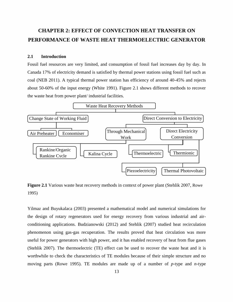
about 50-60% of the input energy (White 1991). Figure 2.1 shows different methods to recover

the waste heat from power plant/ industrial facilities.

Figure 2.1 Various waste heat recovery methods in context of power plant (Stehlik 2007, Rowe

1995)

Yilmaz and Buyukalaca (2003) presented a mathematical model and numerical simulations for

the design of rotary regenerators used for energy recovery from various industrial and air-

conditioning applications. Budzianowski (2012) and Stehlik (2007) studied heat recirculation

phenomenon using gas-gas recuperation. The results proved that heat circulation was more

useful for power generators with high power, and it has enabled recovery of heat from flue gases

(Stehlik 2007). The thermoelectric (TE) effect can be used to recover the waste heat and it is

worthwhile to check the characteristics of TE modules because of their simple structure and no

moving parts (Rowe 1995). TE modules are made up of a number of p-type and n-type

Waste Heat Recovery Methods

Change State of Working Fluid Direct Conversion to Electricity

Air Preheater Economiser Through Mechanical

Work

Direct Electricity

Conversion

Rankine/Organic

Rankine Cycle

Kalina Cycle Thermoelectric

Generators

Thermionic

Generators

Thermal Photovoltaic Piezoelectricity

14

semiconductor materials connected electrically in series and thermally in parallel. A typical

thermoelectric generator (TEG) is made up of a number of TE modules electrically in series

(Rowe 1995). TE modules have many advantages, such as being environmentally friendly and

quiet in operation, and having a long service life (Rowe 1995). However, low conversion

efficiency of TE materials creates difficulty in wide usage (Rowe 1995). The TE effect was first

observed by Seebeck (Wang et al. 2009); when two dissimilar materials are joined together and

junctions are held at two different temperatures then electromotive force is produced (Wang et

al. 2009). The electromotive force depends on an intrinsic property of materials known as the

Seebeck coefficient ( )ΔTV=α . A few years after this experiment, Peltier observed the second

TE effect. When electric current is passed through a junction of two different materials then one

junction liberates the heat and the other absorbs the heat. The Peltier coefficient is defined as

Iq=π P (Wang et al. 2009). The interdependency of both effects dTd=T and T

was derived by Thomson (Lord Kelvin) (Goupil 2011). The Peltier heat is liberated or absorbed

at a junction and is given by TIPq .

During the last several years, various high-performance TE materials have been developed

(Udomsakdigool 2007). To improve the performance of TEG requires making a reasonably good

thermal design, as well as arrangement of TE modules. In early 20th

century, Altenkirch (1911)

established that a good TE material should have large Seebeck coefficient, low thermal

conductivity, and high electrical conductivity. Callen (1947) presented the thermodynamic

theory of the TE phenomenon. Joffe and Stil’bans (1959) introduced a figure of merit as a

parameter to classify different TE materials. Bell (2002) discussed the effect of convective heat

transfer medium on the performance of the TE module and demonstrated criteria for optimum

performance. Xiao et al. (2011) derived a generalised heat transfer model considering convection

heat loss through side walls of TE modules, assuming linear distribution of temperature across

the leg of the TEG. Xiao et al. (2011) concluded that convection heat loss causes a large loss of

heat exergy. One-dimensional analytical solutions of conventional, composite, and integrated

TEG between fixed temperature sources were obtained by Reddy et al. (2013), considering

adiabatic and convective side wall conditions. Regardless of design, increase in hot-side

temperature enhances the performance of TEG. Reddy et al. (2013) also concluded that the

15

composite and integrated TEG extracts more heat compared to the conventional TEG and

reduces rare-element material usage. Chen et al. (2002) studied effect of convection between a

heat source and surface of the TE module to optimize the distribution of heat transfer surface

area. Meng et al. (2012) demonstrated the effect of radiative heat transfer on the performance of

the TEG. A temperature-dependant thermodynamic model was developed by Meng et al. (2012),

considering external irreversibility. Meng et al. (2012) concluded that the temperature-dependent

properties have a large impact on power output and thermal efficiency, especially when the

temperature difference is large. Sahin and Yilbas (2013) considered different optimization

parameters to achieve maximum power output and maximum thermal efficiency. Sahin and

Yilbas (2013) concluded that an increase in thermal conductivity decreases the efficiency and

power output and increases entropy generation rate in TEG. Riffat and Ma (2003) performed a

review of current and potential applications of TE modules. Riffat and Ma (2003) concluded that

where supply of heat is free and abundant (e.g., waste heat or solar energy), efficiency of the TE

system is not a prime concern. The performance of a solar TEG was analysed experimentally by

Goldsmid et al. (1980) in 1980. At that time (Goldsmid et al. 1980), the TEG was made up of

Bi2Te3 and had efficiency of 1%, and could be increased to 3% if proper concentration system

was used. Considering the automotive waste heat recovery from exhaust pipe, Hsiao et al. (2010)

developed 1-D thermal resistance model of TE module. The authors (Hsiao et al. 2010) verified

modeling data with experimental data and calculated maximum power generation of 0.43 W at

290 ºC temperature difference. A TEG system was installed with carburizing furnace at Komatsu

plant to recover the waste heat (Kaibe et al. 2011). A TEG containing 16 TE modules made-up

of bismuth-telluride in groups of 4 was used. Experiments reported total power generation of 250

W with hot surface of temperature of 250 ºC (Kaibe et al. 2011).

The purpose of this work is to explore the performance of the TE device in generator mode

having different temperature dependent transport properties of p- and n- type TE leg with

convection heat transfer losses from the side surfaces to the surrounding environment.

Temperature-dependent Thomson heat is also considered. The junction temperatures of TEG are

function of thermal source and sink temperature and convection heat transfer coefficients

between thermal source and sink to TEG. Modeled equations are initially simplified to 1-D form

16

using appropriate approximations that include 1-D heat transfer, isotropic, and homogeneous

material properties, and decoupled electric and thermal fields. The thermal and electrical contact

resistances between contact surfaces are neglected. Closed forms of solutions are obtained after

solving the simplified 1-D governing equation. Thermal field solutions are used to calculate local

and average entropy generation rates for the TEG. Finally, coupled TE equations are solved

numerically to overcome the implicit problems of the 1-D analytical model to observe the

qualitative results of thermal and electric fields inside the TEG in two dimensions.

2.2 Heat Transfer Modeling

A schematic diagram of the proposed TE heat recovery system is shown in Figure 2.2. This

proposed heat recovery system has different potential arrangements among combustion

chamber/hot fluid pipes, ambient environment, and insulation covering the combustion chamber.

A typical TEG is made up of number of p- and n-type elements connected in series through

copper plate with thermally conductive and electrically insulated ceramic plate on both sides. In

the current study the TEG is placed in such a way that opposite surfaces of ceramic plates face

the combustion chamber and ambient environment, respectively. A unit TEG cell with copper

plate is shown in Figure 2.2 with geometric dimension, coordinate systems, directions of

different heat components, and thermal boundary conditions. The energy transport equation

inside a TEG for a steady state can be expressed as

genq q (1)

where q and genq represent heat generation rate per unit volume, and heat flux vector,

respectively. The continuity of electric charge through the TEG must satisfy

0 J (2)

where J is the electric current density vector. Equations (1) and (2) are coupled by the set of TE

constitutive equations (Antonova et al. 2005) as shown in Eqs. (3) and (4),

TkT Jq

T EJ

(3)

(4)

where is the Seebeck coefficient, k is the thermal conductivity, is the electrical

conductivity, and E is the electric field intensity vector. E can be expressed as , where is

the electric scalar potential (Landau et al. 1984).

17

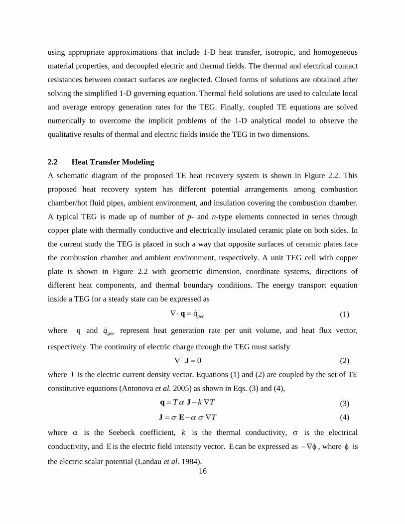
Figure 2.2 Schematic diagram of location of TEG in combustion system and unit TEG cell

Combining Eqs. (1) to (4), the coupled TE equations for energy and electric charge transfers can

be expressed as

JEJ TkT (5)

0 T (6)

where JE represents Ohmic heat (Antonova and Looman 2005). Finally, the entropy generation

equation for TEG can be expressed as (Chakraborty 2006)

JJE 2

2T

T

k

TSgen (7)

where the first term represents the irreversibility due to Ohmic heating, second term is the heat

transfer irreversibility, and the third term is the dissipation due to the Thomson effect. For a

typical TEG shown in Fig. 2b the thermal boundary conditions are as follows:

At the top surface (i.e., 0x ) temperature is 1T , which is the hot junction temperature

At the bottom surface (i.e., lx ) temperature is 2T , which is the cold junction temperature.

Convection heat transfer per unit area from the side surfaces to the surrounding is

)(conv aTThq .

Water /Steam

Pipes

TEGs

Cross-section of combustion

system

x

l

w

p n

Rl

T1

T2

I

qconv

QC

QH

TH

TC

18

It is assumed that the thermal energy enters into the top surface from a thermal source having

constant temperature )( HT and leaves the bottom surface to a thermal sink having constant

temperature )( CT . Heat transfers between the source and the top surface of TEG and sink and

bottom surface of TEG are dominated by convection.

Initially, a simplified 1-D version of the preceding equations is solved to obtain close forms of

analytical solutions. For 1-D analytical heat transfer modeling, a TEG with p-type and n-type

semiconductor legs with load resistance lR (see Fig. 2b) is considered. TE elements having

length l and width w operates between hot and cold junction temperature 1T and 2T ,

respectively. The hot and cold junction temperatures, 1T and 2T , depend on the convection rates

from the surfaces and temperatures of the source )( HT and sink )( CT . A TEG absorbs 1q amount

of heat from the thermal source and rejects 2q amount of heat to the thermal sink. The main

mode of heat transfer through semiconductor leg is conduction, and it is accompanied by Ohmic

heating, Peltier heat generation/liberation at the junctions as well as Thomson heat generation.

The convection heat loss from the side walls of p-type and n-type semiconductor legs to the

ambient environment is also taken into account.

Assuming isotropic and homogeneous material properties and neglecting the thermal and

electrical contact resistances between contact surfaces, the one dimensional heat transfer

equation under steady state condition for semiconductor leg is given by

0)(2

2

2

2

dx

dT

Ak

ITT

Ak

ph

Ak

I

dx

Tda (8)

In Eq. (8), first term is the Fourier heat conduction, second term is the Ohmic heating, third term

is convection heat transfer loss, and fourth term is the Thomson effect.

The general solution to Eq. (8)

xDxDeCeCxT 21

21 (9)

where

2

42

1

D ;

2

42

2

D

(10)

19

;Ak

I ;

Ak

ph

2

2

Ak

IT

Ak

pha

(11)

To calculate 1C and 2C in Eq. (9), convective boundary conditions are applied.

At hot junction and cold junction of TEG, the energy balance equation between thermal source

and thermal sink with TEG can be written as

)( 1

0

TThdx

dTk HH

x

)( 2 CC

lx

TThdx

dTk

(12)

(13)

Substitution of Eqs. (9), (10), and (11) into Eqs. (12) and (13) results in

21

22

1212

2222

1

)(

)()()(

)(

)()(

21

122112

22

22

DDekek

hheeheDkeDkheDkeDk

hheeTT

hDTkDkheDTkeDk

C

lDlD

HC

lDlD

C

lDlD

H

lDlD

HC

lDlD

HC

CCH

lD

H

lD

21

22

1212

1111

2

)(

)()()(

)(

)()(

21

122112

11

11

DDekek

hheeheDkeDkheDkeDk

hheeTT

hDTkDkheDTkeDk

C

lDlD

HC

lDlD

C

lDlD

H

lDlD

HC

lDlD

HC

CCH

lD

H

lD

(14)

(15)

Now, combining heat transfer in semiconductor leg with Peltier heat (which occurs at the

junctions), the heat input at hot junction of TEG is given by

20

2

21

22

1212

1111

1

21

22

1212

2222

21

22

1212

1111

21

22

1212

2222

1

.

)(

)()()(

)(

)()(

)(

)()()(

)(

)()(

)(

)()()(

)(

)()(

)(

)()()(

)(

)()(

21

122112

11

11

21

122112

22

22

21

122112

11

11

21

122112

22

22

D

DDekek

hheeheDkeDkheDkeDk

hheeTT

hDTkDkheDTkeDk

D

DDekek

hheeheDkeDkheDkeDk

hheeTT

hDTkDkheDTkeDk

Ak

DDekek

hheeheDkeDkheDkeDk

hheeTT

hDTkDkheDTkeDk

DDekek

hheeheDkeDkheDkeDk

hheeTT

hDTkDkheDTkeDk

Iq

lDlD

HC

lDlD

C

lDlD

H

lDlD

HC

lDlD

HC

CCH

lD

H

lD

lDlD

HC

lDlD

C

lDlD

H

lDlD

HC

lDlD

HC

CCH

lD

H

lD

lDlD

HC

lDlD

C

lDlD

H

lDlD

HC

lDlD

HC

CCH

lD

H

lD

lDlD

HC

lDlD

C

lDlD

H

lDlD

HC

lDlD

HC

CCH

lD

H

lD

(16)

Equation (16) is the general form of heat transfer equation for a single leg of a TEG applied to

combustion chamber of power plant as a waste heat recovery tool. Consequently, a heat transfer

equation of a single pair of TEG can be obtained by considering respective properties of p-type

and n-type semiconductor legs. Equation (16) reveals that the hot junction temperature )( 1T

depends on the thermal source temperature )( HT and the convection heat transfer coefficient

)( Hh between the thermal source and the hot junction of TEG. In similar manner, the cold

junction temperature )( 2T depends on the thermal sink temperature )( CT and the convection heat

transfer coefficient )( Ch between the cold junction of TEG and the thermal sink. It is important

to note that in the limit of very large convection heat transfer coefficients between the source and

the hot junction and between the sink and the cold junction, the temperatures 1T and 2T approach

the source temperature HT and sink temperature CT .

The net power output of a single TEG is calculated as (Doolittle and Hale, 1984),

VIPo (17)

21

where

inp RITTV )()( 21 (18)

Electric current can be calculated by

li

np

RR

TTI

)()( 21 (19)

The thermal conversion efficiency can be evaluated as

1q

Po (20)

Thermal efficiency is independent of the number of couples, as power output and thermal input

increases linearly with number of modules.

In Eqs. (18) and (19), the temperature at the hot junction )( 1T and the temperature at the cold

junction )( 2T can be evaluated using the boundary conditions ),0( 1TTx and ),( 2TTlx

in Eq. (9).

2.3 Results and discussion

In this section, the performance of a TEG applied to a combustion system as a waste heat

recovery tool is investigated based on the one dimensional analytical solution obtained in the

previous section. The bulk crystalline semiconductor p-type material 25% Bi2Te3 75% Sb2Te3

with 1.75% excess Se and n-type material 75% Bi2Te3 25% Bi2Se3 with copper as a connector

material are used to analyze the performance. The TEG performance characteristics in terms of

thermal efficiency, power output, heat input, and produced electrical current has been studied in

detail. Different operating parameters considered in the current analysis are as follows: Thermal

source temperature (300 K HT 700 K), Thermal sink temperature (260 K CT 320 K), and

surface to surrounding heat transfer coefficient (0 W/m2K h 100 W/m

2K). The dimensions

of the TEG are as follows: length 0.03 m, width 0.01 m, and thickness 0.03 m. The Seebeck

coefficient )( , electrical resistivity )( , and thermal conductivity )(k are specified as

polynomial functions of temperatures as shown in Table 1 (Reddy et al. 2013, Angrist 1982).

These properties are evaluated at average temperature of working range. Load resistance lR is

same as internal resistance iR to get maximum power output.

22

Table 2.1 Temperature dependent TE properties of n-type 75% Bi2Te3 25% Bi2Se3 and p-type

25% Bi2Te375% Sb2Te3 with 1.75% excess Se (Reddy et al. 2013, Angrist 1982)

Property Temperature

Range (ºC)

Polynomial functions of different TE properties in terms of

temperature

n 55025 avgT 517414311

2974

106143.11054021.2103005.1

10574.11026.210517414.1

avgavgavg

avgavg

TTT

TT

p 17020 avgT 515412310

2874

106125.5102189.210265.3

103556.2102663.710084305.2

avgavgavg

avgavg

TTT

TT

450170 avgT 312

2964

1013146.4

108969.4104027.210123379.5

avg

avgavg

T

TT

n 55025 avgT

620

517414312

21086

1049.2

103202.4107176.2102921.7

106044.710324.4103562.9

avg

avgavgavg

avgavg

T

TTT

TT

p 45020 avgT 518414312

2985

109007.81033902.110526.7

1069084.1109785.71014586.1

avgavgavg

avgavg

TTT

TT

nk 10025 avgT 37253 102988.4108823.8103139.42979.1 avgavgavg TTT

400100 avgT 41037

2521

103833.1108004.1

10454.7100936.1101235.8

avgavg

avgavg

TT

TT

550400 avgT 5104734

23

1015322.210950144.410548094.4

0.208700782405.471037663.4

avgavgavg

avgavg

TTT

TT

pk 17020 avgT 5114836

253

100425.410345.11016321.1

1063173.310085.8874746.0

avgavgavg

avgavg

TTT

TT

370170 avgT 38253 10033.710415.110511.484097.1 avgavgavg TTT

450370 avgT 3623 1074356.21069338.36305.194675.234 avgavgavg TTT

23

It is assumed that the thermal energy enters into the top surface of TEG from a thermal source

)( HTT by convection with convection heat transfer coefficient Hh and leaves the bottom

surface of TEG to a thermal sink )( CTT also by convection with convection heat transfer

coefficient Ch . In the special case of very large convection heat transfer coefficients, Hh

and Ch , the top and bottom surface temperatures, 1T and 2T , approach HT and CT (i.e.,

isothermal boundary conditions). The majority of the results presented in this work consider the

influence of convection heat transfer from the side surfaces to the surrounding while the top and

bottom surfaces are exposed to a high convective environment (i.e., nearly isothermal).

However, the effect of convection from the source to the top surface and from the bottom surface

to the sink is considered for limited cases, presented at the end of this work.

Temperature Distribution

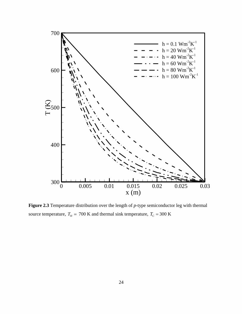
Figures 2.3 and 2.4 show the temperature distribution along the longitudinal directions of a p-

type and n-type semiconductor leg at different values of the surface to surrounding convection

heat transfer coefficients. The thermal source and the thermal sink temperatures are kept constant

at 700 K and 300 K, respectively. For a given amount of the surface to surrounding convection

loss, it is observed that the difference in the temperature gradients of p-type and n-type legs is

negligible. This negligible difference is due to the minimal difference in the TE properties

between p- and n-type TE legs. However, it is observed from these plots that the convection

losses from the side surfaces to the surrounding have larger impact on the temperature

distribution. At higher values of the convection heat transfer coefficients, a larger amount of heat

removal occurs from the side surfaces; this, in turn, causes a rapid temperature drop along the leg

when compared to the nearly adiabatic side surface temperature profile (i.e., h = 0.1 W/m2K). As

shown later, convection heat losses affect the heat input to the TEG and thermal efficiency of the

TEG significantly.

24

x (m)

T(K

)

0 0.005 0.01 0.015 0.02 0.025 0.03300

400

500

600

700

h = 0.1 Wm-2K

-1

h = 20 Wm-2K

-1

h = 40 Wm-2K

-1

h = 60 Wm-2K

-1

h = 80 Wm-2K

-1

h = 100 Wm-2

K-1

Figure 2.3 Temperature distribution over the length of p-type semiconductor leg with thermal

source temperature, HT 700 K and thermal sink temperature, CT 300 K

25

x (m)

T(K

)

0 0.005 0.01 0.015 0.02 0.025 0.03300

400

500

600

700

h = 0.1 Wm-2

K-1

h = 20 Wm-2

K-1

h = 40 Wm-2

K-1

h = 60 Wm-2

K-1

h = 80 Wm-2

K-1

h = 100 Wm-2

K-1

Figure 2.4 Temperature distribution over the length of n-type semiconductor leg with thermal

source temperature, HT 700 K and thermal sink temperature, CT 300 K

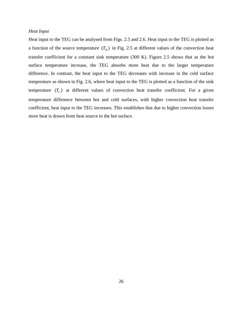
26

Heat Input

Heat input to the TEG can be analysed from Figs. 2.5 and 2.6. Heat input to the TEG is plotted as

a function of the source temperature )( HT in Fig. 2.5 at different values of the convection heat

transfer coefficient for a constant sink temperature (300 K). Figure 2.5 shows that as the hot

surface temperature increase, the TEG absorbs more heat due to the larger temperature

difference. In contrast, the heat input to the TEG decreases with increase in the cold surface

temperature as shown in Fig. 2.6, where heat input to the TEG is plotted as a function of the sink

temperature )( CT at different values of convection heat transfer coefficient. For a given

temperature difference between hot and cold surfaces, with higher convection heat transfer

coefficient, heat input to the TEG increases. This establishes that due to higher convection losses

more heat is drawn from heat source to the hot surface.

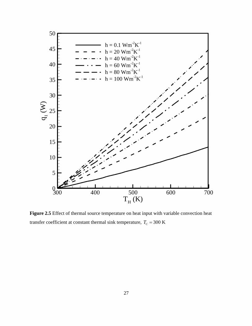
27

TH

(K)

q1

(W)

300 400 500 600 7000

5

10

15

20

25

30

35

40

45

50

h = 0.1 Wm-2

K-1

h = 20 Wm-2

K-1

h = 40 Wm-2

K-1

h = 60 Wm-2

K-1

h = 80 Wm-2

K-1

h = 100 Wm-2

K-1

Figure 2.5 Effect of thermal source temperature on heat input with variable convection heat

transfer coefficient at constant thermal sink temperature, CT 300 K

28

TC

(K)

q1

(W)

260 270 280 290 300 310 32010

15

20

25

30

35

40

45

50

55

60

65

h = 0.1 Wm-2

K-1

h = 20 Wm-2

K-1

h = 40 Wm-2K

-1

h = 60 Wm-2

K-1

h = 80 Wm-2

K-1

h = 100 Wm-2K

-1

Figure 2.6 Effect of thermal sink temperature on heat input with variable convection heat

transfer coefficient at constant thermal source temperature, HT 700 K

29

Power Output

Figure 2.7 presents the power output as functions of source and sink temperatures. As source

temperature increases for a constant sink temperature, power output also increases. In contrast,

the power output decreases as cold surface temperature increases for a fixed value of the source

temperature. One can observe from Eqs. (17) and (18) that the temperature difference has

significant impact on power output. As temperature difference increases, power output also

increases. The same equation verifies that power output is independent of the convection heat

transfer losses from the side surfaces to the surrounding.

30

TH

(K)

Po

(W)

300 400 500 600 7000

0.5

1

1.5

2

TC=270 K

TC=280 K

TC=290 K

TC=300 K

Figure 2.7 Power generation as a function of thermal source temperature at different thermal

sink temperature

31

Thermal Efficiency

Thermal efficiency is plotted as a function of hot surface temperature with constant cold surface

temperature in Fig. 2.8 at different values of convection heat transfer coefficient. The thermal

efficiency plot, as shown in Fig. 2.8, demonstrates that for a constant sink temperature (300 K)

with increment in the hot surface temperature the thermal efficiency of TEG increases. In

contrast, for a constant source temperature, the thermal efficiency of the TEG increases with

decrease in the cold surface temperature as shown in Fig. 2.9, where thermal efficiency is plotted

as a function of the cold surface temperature at different convection heat transfer coefficient and

constant source temperature (700 K). A larger magnitude of the T gives greater thermal

efficiency, provided that material used in TEG can withstand upper limits of temperature

exposure. In combustion system, the hot surface temperature can be easily maintained at constant

values due to the constant heat generation in the chamber. Figures 2.8 and 2.9 also establish the

effect of the surface to surrounding convection heat losses on the thermal efficiency. For a given

temperature difference between hot and cold surfaces, an increase in the convection heat transfer

coefficient decreases the thermal efficiency of the TEG. The irreversible convection process

causes larger amount of heat loss to ambient environment, so it suggests that less heat is

available to convert into electricity and this leads to low thermal efficiency.

32

TH

(K)

300 400 500 600 7000

2

4

6

8

10

12

h = 0.1 Wm-2K

-1

h = 20 Wm-2K

-1

h = 40 Wm-2K

-1

h = 60 Wm-2K

-1

h = 80 Wm-2K

-1

h = 100 Wm-2

K-1

Figure 2.8 Effect of thermal source temperature on thermal efficiency with variable convection

heat transfer coefficient at constant thermal sink temperature, CT 300 K

33

TC

(K)

260 270 280 290 300 310 3202

4

6

8

10

12

h = 0.1 Wm-2

K-1

h = 20 Wm-2

K-1

h = 40 Wm-2K

-1

h = 60 Wm-2

K-1

h = 80 Wm-2

K-1

h = 100 Wm-2

K-1

Figure 2.9 Effect of thermal sink temperature on thermal efficiency with variable convection

heat transfer coefficient at constant thermal source temperature, HT 700 K

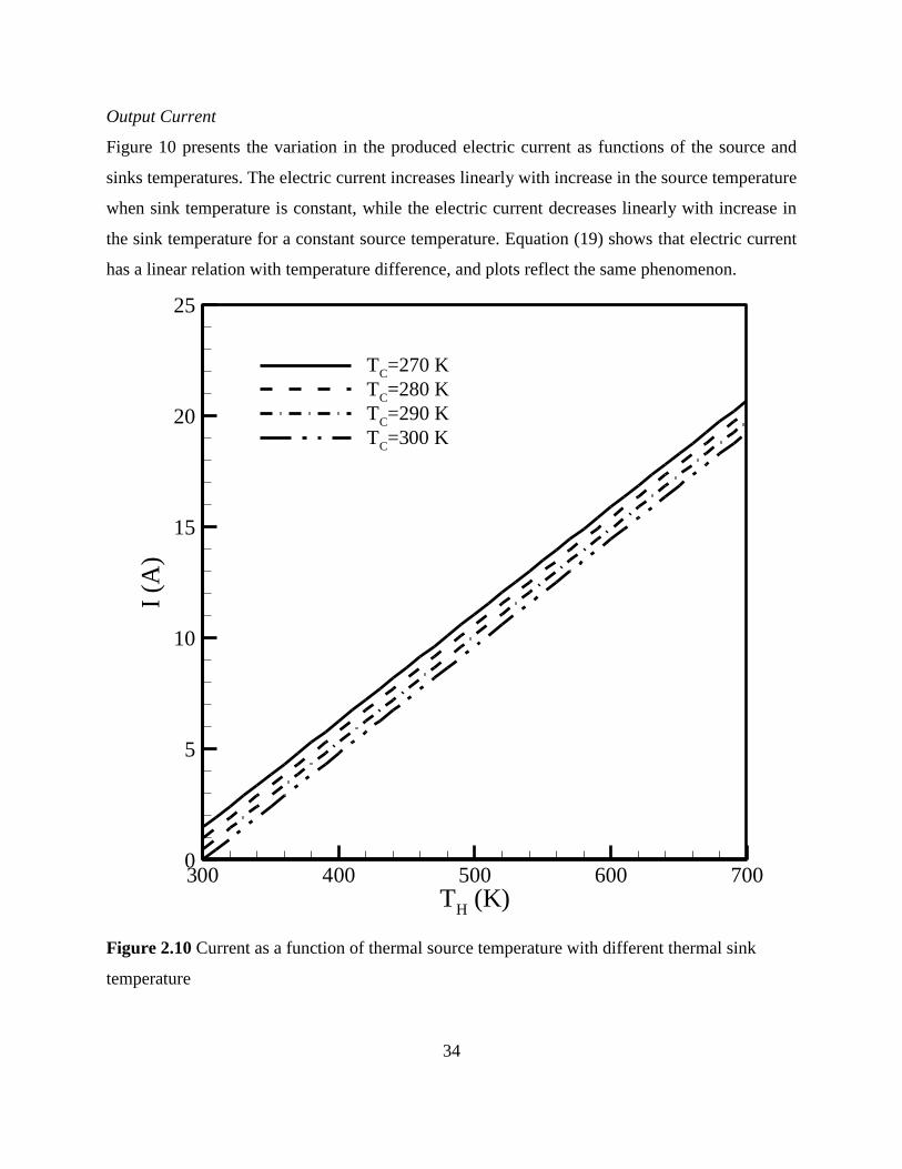
34

Output Current

Figure 10 presents the variation in the produced electric current as functions of the source and

sinks temperatures. The electric current increases linearly with increase in the source temperature

when sink temperature is constant, while the electric current decreases linearly with increase in

the sink temperature for a constant source temperature. Equation (19) shows that electric current

has a linear relation with temperature difference, and plots reflect the same phenomenon.

TH

(K)

I(A

)

300 400 500 600 7000

5

10

15

20

25

TC=270 K

TC=280 K

TC=290 K

TC=300 K

Figure 2.10 Current as a function of thermal source temperature with different thermal sink

temperature

35

Irreversible Convection Heat Transfer

The effect of the surface to surrounding convection heat transfer coefficient on thermal

efficiency is demonstrated in Fig. 2.11. It is observed from the plot that the convection heat

losses from the side surfaces have more impact on thermal efficiency. For a given temperature

difference between the source and sink, thermal efficiency decreases as convection heat transfer

coefficient increases. Heat input increases with increasing rate of side wall convection (Fig. 2.5);

however, the power output remains nearly invariant (Eqs. (17) and (18)) with increase in side

wall convection heat transfer coefficient. Therefore, efficiency decreases as side wall convection

heat transfer coefficient increases for a constant temperature difference.

The effect of convections between the thermal source and the top surface and between the sink

and the bottom surface of TEG on thermal efficiency is shown in Figs. 2.12 and 2.13 for the

adiabatic side wall condition (Fig. 2.12) and convection from the side walls with h = 10 W/m2K

(Fig. 2.13). The temperatures of the source and sink are 700 K and 300 K, respectively. A lower

convection heat transfer coefficient between thermal source and sink to TEG leads to low

thermal efficiency. An introduction of convection resistances between the thermal source and the

top surface and between the sink and the bottom surface of TEG create more irreversibility to the

TEG, which causes an efficiency reduction. Isothermal top and bottom surfaces represent a

special case of zero convection resistance and the thermal efficiency is maximum for such case,

as can be observed from Fig. 2.12 ( 410 CH hh W/m2K). Both heat input and power output

decrease with decreasing Hh and Ch (higher convection resistances), which, in turn, lower the

efficiency of the TEG. An introduction of the convection losses from the side surfaces lower the

efficiency further, as can be seen from Fig. 2.13.

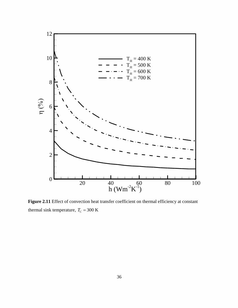
36

h (Wm-2

K-1

)

20 40 60 80 1000

2

4

6

8

10

12

TH

= 400 K

TH

= 500 K

TH

= 600 K

TH

= 700 K

Figure 2.11 Effect of convection heat transfer coefficient on thermal efficiency at constant

thermal sink temperature, CT 300 K

37

I (A)

5 10 15 200

2

4

6

8

10

12

hC

= hH

= 50 Wm-2

K-1

hC

= hH

= 100 Wm-2

K-1

hC

= hH

= 103

Wm-2K

-1

hC

= hH

= 104

Wm-2

K-1

Figure 2.12 Effect of convections between the thermal source and the top surface and between

the sink and the bottom surface of TEG on thermal efficiency when HT 700 K and CT 300 K

with adiabatic side wall condition

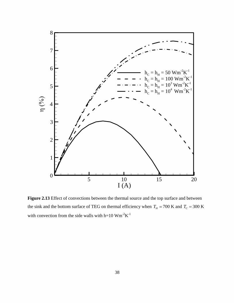
38

I (A)

5 10 15 200

1

2

3

4

5

6

7

8

hC

= hH

= 50 Wm-2K

-1

hC

= hH

= 100 Wm-2

K-1

hC

= hH

= 103

Wm-2K

-1

hC

= hH

= 104

Wm-2

K-1

Figure 2.13 Effect of convections between the thermal source and the top surface and between

the sink and the bottom surface of TEG on thermal efficiency when HT 700 K and CT 300 K

with convection from the side walls with h=10 Wm-2

K-1

39

Irreversibility Analysis

Entropy is produced by the irreversible processes in TE devices (Yilbas and Pakdemirli 2005,

Sekulica 1986), and, in this respect a typical TEG is no exception. If these irreversible processes

could be eliminated, entropy production would be reduced to zero (Bermejo et al. 2013). In such

cases the limiting value of the Carnot efficiency for a TEG would be obtained. Unfortunately, it

is impossible to reduce the irreversibilities of a system to zero. Therefore, during the operation,

the performance of the TEG can be further improved through the minimization of the

thermodynamic losses. One of the methods to maximize the thermal efficiency of the TEG is to

minimize the entropy generation rate. Therefore, entropy generation analysis is a very important

tool to understand the performance of the TEG.

The general expression of the local entropy generation rate, given by Eq. (7), can be simplified to

obtain a 1-D entropy generation rate equation for the present problem as shown here:

2

2

,

2

2

)( TT

k

TA

IS

np

gen

(21)

Expression of the temperature distribution (Eq. (9)) is used to obtain the preceding expression of

the local entropy generation rate. Note that the spatial dependency of the Seebeck coefficient

( ) in the last term of Eq. (7) is neglected to obtain Eq. (21), assuming a homogeneous

material. Equation (21) is the volumetric local entropy generation rate (W/m3K), where first term

represents the irreversibility due to the Ohmic heating and the second term represents

irreversibility due to the temperature gradient. The volume averaged entropy generation rate

( genS ) can be obtained from the following equation:

dVdx

dT

T

k

TA

I

VS

np

gen

2

2

,

2

21 (22)

For the constant cross-sectional area of TE legs, Eq. (22) can be further simplified to

dxdx

dT

lT

k

TA

IS

Lnp

gen

0

2

2

,

2

2

. (23)

Above equation can be written in the dimensionless form,

dxTlT

k

TA

I

k

lS

L

np

np

gen

0

2

2

,

2

2

,

2

(24)

40

wher

2

,

lk

SS

np

gengen (25)

In Eq. (24), the temperature gradient contained in the second term on the right side can be

evaluated by using Eqs. (9), (14), and (15). Finally average entropy generation over the entire

volume of a TEG leg can be evaluated in non-dimensional form as shown here:

21

22

2

2

21

2

2

2

22121

2

21

2

1

22

1

2

1

2

2

2

2

21

2

2212121

2

1

2

1

2

1

2

,

2

2

,

2

2

4

4

2221

11

DD

eDCDeDCeDDCC

eDDCeDCDC

DDCDDCCDDCDC

lT

k

TA

I

k

lS

lDlDlDlD

lDlD

np

np

gen (26)

The simplified expressions for 1C and 2C are defined already in Eqs. (14) and (15). Similarly,

simplified expressions for 1D and 2D are defined in Eq. (10).

The volume averaged dimensionless entropy generation rate, as presented in Eq. (26), is plotted

as a function of the source temperature for different values of the convection heat transfer

coefficient in Fig. 2.14. The sink temperature is assumed constant and equal to

300 K. For a small temperature difference between the source and sink, the magnitude of the heat

transfer contribution to the entropy generation is negligible. For this special case, the irreversible

Ohmic heating dominates the overall entropy generation rate, which is relatively small in

magnitude when compared with the heat transfer irreversibility. Therefore, small values of the

entropy generation rate are observed at values of the source temperatures. Note that for a very

special case of isothermal system ( 0T ) heat transfer irreversibility is zero. An increase in

the source temperature increases the entropy generation rate as observed from Fig. 2.14. Higher

temperature difference between the source and sink brings more heat to the TEG along the larger

finite temperature difference, which is naturally irreversible. An introduction of the surface to

surrounding convection increases this irreversibility further. Therefore, a higher entropy

generation rate is observed in Fig. 2.14 at higher values of the convection heat transfer

coefficient for a given temperature difference between the source and sink. For small

temperature difference between the source and sink, the variation in the magnitude of the entropy

41

generation rate is insignificant with increasing values of the convection heat transfer coefficient.

In contrast, a larger variation in the entropy generation rate is observed with convection heat

transfer coefficient when temperature difference is relatively large.

42

TH

(K)

S* g

en

400 500 600 7000

5

10

15h = 0.1 Wm

-2K

-1

h = 20 Wm-2

K-1

h = 40 Wm-2K

-1

h = 60 Wm-2

K-1

h = 80 Wm-2

K-1

h = 100 Wm-2

K-1

||

Figure 2.14 Entropy generation rate as a function of thermal source temperature at different

convection heat transfer coefficients with constant thermal sink temperature, CT 300 K

43

2-D Numerical Results

Equations (5) and (6) are the modeled differential equations for the coupled thermal and electric

fields. Until this point, a simplified 1-D version of the energy equation (Eq. (5)) has been used to

describe the characteristic features of the TEG used in this work. In this section, some selected

parameters of the TEG are evaluated by solving the 2-D coupled thermal-electric equations (Eqs.

(5) and (6)). Equations (5) and (6) are solved using a finite element method. A description of the

discretization and solution techniques is available in Mahmud and Pop (2006). Properties of p-

and n-type semiconductor legs were approximated at the average temperature of working range

using relations given in Table 2. For the numerical analysis, the hot junction temperature (= 700

K) and the cold junction temperature (= 300 K) are kept constants. Computations are carried out

for two different cases of TEG side wall heat transfer boundary conditions: adiabatic and

convective heat transfer. All geometrical parameters are same as 1-D analysis. For adiabatic side

walls of p and n-type semiconductor legs, Figures 11(a) and 11(b) present the thermal and

electric potential field results. Figure 11(a) presents the temperature and heat flow results while

Figure 11(b) reveals the electric scalar potential and current flow. Surface to surrounding

convection is introduced next, and the entire field results are repeated for h = 20 W/m2K and

presented graphically in Figs. 2.17 and 2.18. In order to carry out the numerical simulation, both

terminals (the bottom ends of the p- and n-leg) are connected directly using a strip of material

having known electrical resistance to approximate the external load resistance. For a particular

TE leg, temperature remains nearly constant at a given location of distance x when 0h

W/m2K. However, the location of the same isothermal line is slightly different at p- and n-leg

due to the dissimilar properties. In the absence of the surface to surrounding convection, the heat

flux lines are parallel in both p - and n- leg and uniformly distributed over the cross-section of

the legs. An introduction of the surface to the surrounding convection introduces the non-

linearity in the temperature distribution, as observed from Fig. 2.17. At a given x location,

surface of a TE leg is cooler than the core due to the heat removal by convection. The heat flux

lines are no longer parallel in both p- and n-leg and a non-uniform distribution is observed. A

certain portion of the heat, entering the top surface of the TEG, is leaving through the side

surfaces by convection, as evidenced by the heat flux lines terminated at the vertical side

surfaces of the legs. Due to the coupled TE effect, potential difference is established in the leg

44

which drives an electric current through the TEG. For a particular TE leg, electric potential

remains nearly constant at a given location of distance x when h = 0 W/m2K. However, non-

linear potential distribution is observed when h = 20 W/m2K.

45

320320

340

360360

380

400

420

440

460

480

500

520

540

560

580580

600

620620

640

660

680

320

340

360

380

400

420

440

460 460

480

500

520

540 540

560

580

600

620 620

640

660

680

Figure 2.15 Temperature distribution in TEG with adiabatic boundary conditions at vertical

walls of semiconductor legs

46

-0.009

-0.008

-0.007

-0.006-0.006

-0.005

-0.004

-0.003

-0.002

-0.001

0

0.001

0.0020.003

0.0040.005

0.0060.007

-0.009-0.008

-0.007

-0.006 -0.006

-0.005

-0.004

-0.003

-0.002

-0.001

0

0.001

0.002

0.003 0.003

0.004

0.005

0.006

0.007 0.007

Figure 2.16 Electrical potential in TEG with adiabatic boundary conditions at vertical walls of

semiconductor legs

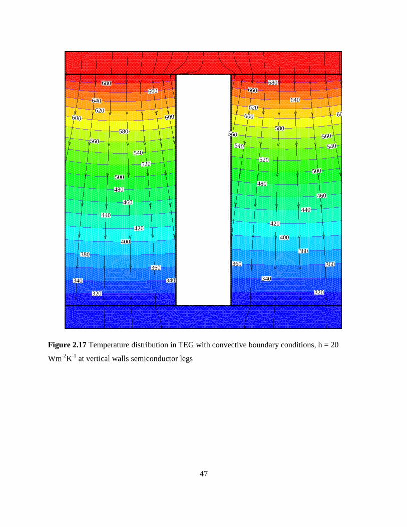
47

320

340340

360

380

400

420

440

460

480

500

520

540

560

580

600600

620

640

660

680

320

340

360 360

380

400

420

440

460

480

500

520

540 540

560 560

580

600 600620

640

660

680

Figure 2.17 Temperature distribution in TEG with convective boundary conditions, h = 20

Wm-2

K-1

at vertical walls semiconductor legs

48

-0.009

-0.008

-0.007

-0.006

-0.005

-0.004

-0.003

-0.002

-0.001

0

0.0010.001

0.002

0.003

0.004

0.005

0.006

0.007

-0.009 -0.009

-0.008

-0.0

08

-0.007

-0.006

-0.005

-0.004-0.004-0.003

-0.002

-0.001

00.001

0.0020.0030.004

0.0050.006

0.007

Figure 2.18 Electrical potential in TEG with convective boundary conditions, h = 20 Wm-2

K-1

at


49

Comparison and Validation

In this section, a comparison of current results with the similar type of results (available in the

literature) is presented. Reddy et al. (2013) performed a theoretical performance study of

conventional, composite, and integrated TE devices applicable to waste heat recovery system.

Performance results in Reddy et al. (2013) are presented for h = 0 - 1000 W/m2K with hot

surface temperature 450 K and cold surface temperature 300 K. By using the conventional TE

device dimensions, variable material properties, and thermal/electric boundary conditions

(Reddy et al. 2013), thermal efficiencies are calculated for five different hot to cold surface

temperature differences and presented in Table 2.2. Results presented in Table 2.2 are for a

single unit of TEG. Thermal efficiencies obtained using the efficiency equation of current work

show good agreement with the results obtained by Reddy et al. (2013). Note that the numerical

values available in the third column in Table 2.2 are extracted manually from Figure 4 of Reddy

et al. (2013) which is for h = 0 W/m2K with hot surface temperature 300-550 K and cold surface

temperature 300 K. An additional comparison is presented in Fig. 2.19, where heat input, power

output, and thermal efficiency results are obtained from section 4.4.3 of Angrist (1982) for an

optimized TEG and compared with the results obtained from equations derived in the current

work. Angrist (1982) used an adiabatic side boundary condition. Figure 2.19 shows good

agreement between current results and results obtained by Angrist (1982). Figure 2.20 presents

the comparison between analytical results and numerical simulation carried out in this work. The

plot shows good agreement of results between the developed analytical model and numerical

simulation at lower convection heat transfer coefficient. In contrary, discrepancy grows as the

convection heat transfer coefficient increases.

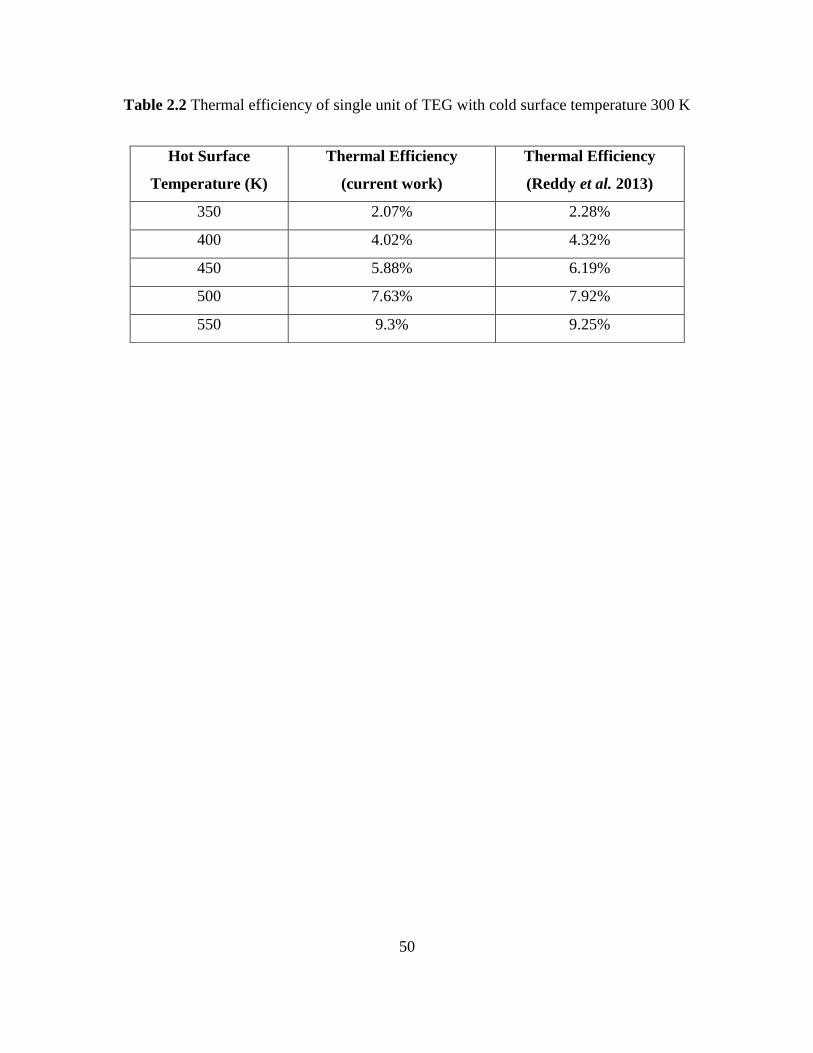
50

Table 2.2 Thermal efficiency of single unit of TEG with cold surface temperature 300 K

Hot Surface

Temperature (K)

Thermal Efficiency

(current work)

Thermal Efficiency

(Reddy et al. 2013)

350 2.07% 2.28%

400 4.02% 4.32%

450 5.88% 6.19%

500 7.63% 7.92%

550 9.3% 9.25%

51

T (oC)

50 100 150 200 250 300 350 4000

3

6

9

12

15

Heat input (current work)

Power output (current work)

50 100 150 200 250 300 350 4000

3

6

9

12

Efficiency (current work)

50 100 150 200 250 300 350 4000

3

6

9

12

Efficiency (Angrist 1982)

q1

an

dP

o(W

)

0

3

6

9

12

15

Heat input (Angrist 1982)

Power output (Angrist 1982)

Figure 2.19 Comparison of heat input, power output, and thermal efficiency obtained from the

current work with the similar results available in (Angrist 1982)

52

x (m)

T(K

)

0 0.005 0.01 0.015 0.02 0.025 0.03300

400

500

600

700

h = 0.1 Wm-2

K-1

(analytical)

h = 25 Wm-2

K-1

(analytical)

h = 50 Wm-2

K-1

(analytical)

h = 0.1 Wm-2

K-1(numerical)

h = 50 Wm-2K

-1(numerical)

h = 25 Wm-2K

-1(numerical)

Figure 2.20 Comparison of analytical and numerical results in terms of temperature distribution

over the p-type semiconductor leg

53

2.4 Conclusion

This research has developed 1-D analytical and numerical 2-D numerical analyses of TEG

applied to waste heat recovery from combustion system in power plants. Based on fundamental

theories of TE phenomenon and energy balance, detailed 1-D heat transfer modeling is derived

involving Fourier heat conduction, ohmic heating, and convection heat transfer losses, and

Peltier, Seeback and Thomson effects. In addition to this, convective boundary conditions have

been considered between thermal source and sink to TEG. The influences of thermal source and

sink temperatures and convection heat transfer coefficient on various performance parameters of

TEG such as power output, heat input, thermal efficiency, and electric current have been studied.

An increase or decrease in thermal source and sink temperature has a considerable effect on the

performance of TEG. As temperature differential T increases, power output and thermal

efficiency increases. It is also found that the convection heat transfer coefficient has extensive

impact on the performance of TEG. Escalation in heat input and drop in thermal efficiency are

observed with increment in convection heat transfer coefficient. The results also show that

increment in convection heat transfer coefficient increases entropy generation and thus destroy

the exergy. Finally, a 2-D mathematical model is solved numerically to observe qualitative

results of thermal and electric fields inside the TEG. Field results of numerical analysis match to

that of 1-D analytical results. Numerical results also prove that the presence of an irreversible

heat convection process does cause a large amount of heat loss which matches with 1-D

analytical result. A waste heat TEG needs to be designed carefully, considering the effect of

internal and external irreversible convection losses.

54

2.5 Nomenclature

A cross-sectional area (m2)

1C a parameter (see Eq.(14))

2C a parameter (see Eq.(15))

1D a parameter (see Eq.(10))

2D a parameter (see Eq.(10))

E electric field intensity vector (Vm-1

)

h convection heat transfer coefficient (Wm-2

K-1

)

I electric current (A)

J electric current density (Am-2

)

k thermal conductivity (Wm-1

K-1

)

l length of p type and n type semiconductor material respectively (m)

p perimeter (m)

P electric power output (W)

q heat or energy for TEG (W)

q heat flux (Wm-2

)

Q heat or energy for thermal source and sink (W)

.

q heat generation rate per unit volume (Wm-3

)

R electrical resistance (Ω)

S entropy (Wm-3

K-1

)

S volume averaged entropy (WK-1

)

T temperature (K)

V voltage (V), volume (m3)

w width (m)

x coordinate (m)

Greek Symbols

Seebeck coefficient (VK-1

)

a parameter (see Eq. (11))

a parameter (see Eq.(11)))

55

efficiency (%)

Peltier coefficient (V)

electrical resistivity (Ωm)

electrical conductivity (Sm-1

)

Thomson coefficient (VK-1

)

a parameter (see Eq.(11))

electric scalar potential (V)

Subscripts

1 hot junction of TEG

2 cold junction of TEG

a atmospheric condition

avg average temperature

C thermal/heat sink

conv convection

gen generation

H thermal/heat source

i internal

l external load

o output

n n-type semiconductor material

P Peltier effect

p p-type semiconductor material

Superscripts

* dimensionless form

56

CHAPTER 3: NUMERICAL SIMULATION OF NANOSTRUCTURED

THERMOELECTRIC GENERATOR CONSIDERING SURFACE TO

SURROUNDING CONVECTION

3.1 Introduction

The research and development in nanostructured thermoelectric (TE) systems have gathered

considerable attention due to their potential applications in direct electricity generation,

refrigeration, and air-conditioning. TE systems can largely be classified as thermoelectric

generator (TEG) and thermoelectric cooler (TEC). The TEG converts heat into electricity and

TEC converts electricity into heating/cooling based on Seebeck and Peltier effects, respectively.

TE systems are solid state heat engines/refrigerators which are robust, silent, compact, and

environment friendly. TE systems are made up of numbers of p-type and n-type semiconductor

elements connected electrically in series and thermally in parallel. The TEC has a wide range of

applications; for example, electronic cooling, laser diode cooling, military garment, laboratory

cold plates, and automobile seat cooler. In a similar manner, TEG has various applications in

military, deep space vehicles, remote power sources for inhabitable places, solar and waste heat

power generator. Liquid cooling of CPU using TE was proposed and experimentally investigated

considering different material and size of the heat sinks (Naphon and Wiriyasart 2009). Huang et

al. (2010) have discussed TE cooling of electronic equipment experimentally and analytically.

The results determined that the integration of water-cooling with TE is helpful to increase the

performance of electronic equipment. In order to address the site specific on-demand cooling of

hot spot in microprocessor (Sullivan et al. 2012), a numerical simulation that includes heat

spreader, thermal interface material, chip, and nine TECs was carried out considering steady

state and transient analysis. Sullivan et al. (2012) concluded that transient cooling with square

root current pulse is most effective with 10°C cooling. Wang (2013) has proposed and

investigated experimentally the TEG using waste heat of the Light-Emitting Diodes. Results

reported by Wang (2013) investigated power output of TEG using waste heat of the Light-

Emitting Diodes (LED). Experiments of Wang (2013) showed 160 mW of power output from

TEG with 6 W of input power to LED. Recently, Hsiao et al. (2010) studied the performance of

TE modules as a waste heat recovery tool from an automobile engine using a one-dimensional

57

thermal resistance model and compared their model with experimental data. Results (Hsiao et al.

2010) showed that the performance of a TE module on the exhaust pipe performs better

compared to a TE module on the radiator system. Rezania et al. (2012) have studied the effect of

cooling power on the performance of a TEG. Rezania et al. (2012) determined the optimum

coolant flow rate for maximum power output for the TEG. For example, temperature difference

of 10 K gives maximum power output of 0.035 W with coolant flow rate of 0.07 l/min (Rezania

et al. 2012). One-dimensional analytical solutions of conventional, composite, and integrated

TEG have been carried out by Reddy et al. (2013) considering adiabatic and convective side wall

conditions. Regardless of TEG design, an increment in the hot side temperature enhances the

performance of TEG systems (Reddy et al.2013). Reddy et al. (2013) concluded that composites

and integrated TEG extracts more heat compared to conventional TEG and reduces rare-element

material usage. Gou et al. (2010) investigated the performance of low temperature waste heat

TEG using one-dimensional analytical simulations and experiments. They (Gou et al. 2010)

concluded that in addition to increasing the waste heat temperature and number of modules in

series, expanding the heat sink surface area and enhancing the cold side heat transfer in proper

ranges can have dramatic effects on TEG’s performance. A three dimensional numerical model

of TEG applied to fluid power systems is developed by Chen et al. (2011) and their numerical

simulation performed with ANSYS shows fairly good match with experimental results. In

addition to this, Chen et al. (2011) concluded that convection heat transfer losses increase the

heat input to TEG thus reduces the thermal efficiency of TEG. A three-dimensional coupled

numerical simulation of integrated TE device was carried out by Reddy et al. (2012) to check the

effects of Reynolds number and fluid temperature on performance of an integrated TEG system.

Reddy et al. (2012) found that higher Reynolds number enhances the heat transfer and thus leads

to higher power output of TEG. Zhou et al. (2013) have developed simple and coupled field

model with former considering Navier-stokes and energy equations with continuity equation and

later with different TE effects such as Seebeck, Peltier, and Thomson effect. Zhou et al. (2013)

reported overall TEG efficiency of 3.5% with temperature difference of 80 K. Baranowski et al.

(2012) have developed mathematical model for solar TEG which can provide analytical solutions

of device efficiency with temperature dependant properties. They (Baranowski et al. 2012) have

also showed that considering currently available materials, total efficiency of 14.1% is possible

58

with cold and hot side temperature of 100 °C and 1000 °C, respectively. Baranowski et al.

(2012) also concluded that if figure of merit (ZT) reaches to 2 then TEG efficiency of 25% can

be obtained, for the cold and hot side temperature of 100 °C and 1000 °C, respectively.

Altenkirch (1911) introduced figure of merit, ZT as a parameter to classify different materials.

The performance of TE materials are characterised by a dimensionless parameter ‘figure of

merit’, TZT )( 2 , where is the Seebeck coefficient, is the electrical conductivity, and

is the thermal conductivity. The current ZT value of the best available TE materials is 1 at

room temperature (Vineis et al. 2010). Slack (1995) has described that good TE materials need

to have low thermal conductivity. In addition to this, Slack (1995) described that the best TE

material would behave as “Phonon Glass Electron Crystal (PGEC)”; that is, it would have

thermal properties of glass like material and electrical properties of crystalline material. Recent

advancements in the field of nanotechnology (Vineis et al. 2010) have opened the door for

further improvements of ZT for the TE materials. The expression of the figure of merit,

TZT )( 2 , evidently indicates that one of the methods to increase figure of merit is to

reduce the thermal conductivity of the TE material. Thermal conductivity is the sum of two

contributions: electrons and hole transporting the heat )( E and phonons traveling through the

lattice )( L (Tritt 2001). The electronic part of thermal conductivity )( E is related to the

electrical conductivity as par the Wiedemann-Franz law (Tritt 2001) as shown in Eq. (1),

TLoE (1)

where, oL is the Lorentz number and for metals it is equal to (Tritt 2001),

8

2

22

1045.23

e

kLo V

2K

-2 (2)

where, k is the Boltzmann constant ( 231038.1 JK-1

) (Tritt 2001) and e is the electron charge

( C1060.1 19 ) (Godart et al. 2009). The expression of the figure of merit can be written in terms

of Lattice conductivity )( L and electronic conductivity )( E as shown below (Tritt 2001),

LE

E

oLZT

2

. (3)

One method to enhance ZT is the inclusion of nanoparticles into the bulk TE materials which can

lead to low lattice thermal conductivity (Ma et al. 2013). Poudel et al. (2008) achieved ZT value

59

of 1.4 at 373 K by hot-pressing of nanopowders of Bi2Te3 and Sb2Te3 under Argon )(Ar

atmosphere. The enhanced ZT was due to the significant decrease in the lattice thermal

conductivity of material. Zhao et al. (2008) fabricated Bi2Te3 with various amount of nano SiC

particles using mechanical alloying and spark plasma sintering and tested the TE and mechanical

properties. Their results showed an improvement in ZT from 0.99 to 1.04 with an inclusion of

0.1% vol% SiC particles. Li et al. (2009) obtained ZT of 1.43 for double-doped 124SbCo

skutturedites using Indium )(In and Cerium )(Ce doping. The attractive results achieved using

nanotechnology has encouraged researchers to include nanoparticle-doped TE materials for

various low potential heat recovery applications; for example, solar TEG and automobile exhaust

heat recovery. Kraemer et al. (2011) have proposed novel solar TEG with glass vacuum

enclosure considering nanostructured TE materials. The developed solar TEG achieved

maximum efficiency of 4.6% with solar flux of 1000 W/m2 condition. McEnaney et al. (2011)

developed a novel of TEG. They (McEnaney et al. 2011) placed high performance

nanostructured material in evacuated tube with selective absorber and achieved an efficiency of

5.2%. It is quite evident that nanostructured TE materials can increase the performance of TE

systems.

It is quite clear from the above discussion that in future nanostructured TE materials will play a

significant role as a direct energy conversion tool from low potential sources. It is necessary to

understand wide range of characteristic features of newly developed TE materials. Such

characteristic features include heat transport and electric potential. The existing literature on the

numerical simulation of nanostructured TEG is very limited. In this work, performance of

nanostructured TEG is evaluated using 2D numerical simulation. The temperature dependent

thermophysical and electrical properties of nanostructured TE material, surface to surrounding

convection heat transfer losses, and Thomson effect are included in the current model. The field

plots of heat and current are presented with different convection heat transfer coefficients.

Numerical results are compared with that of one dimensional analytical results in terms of

current produced.

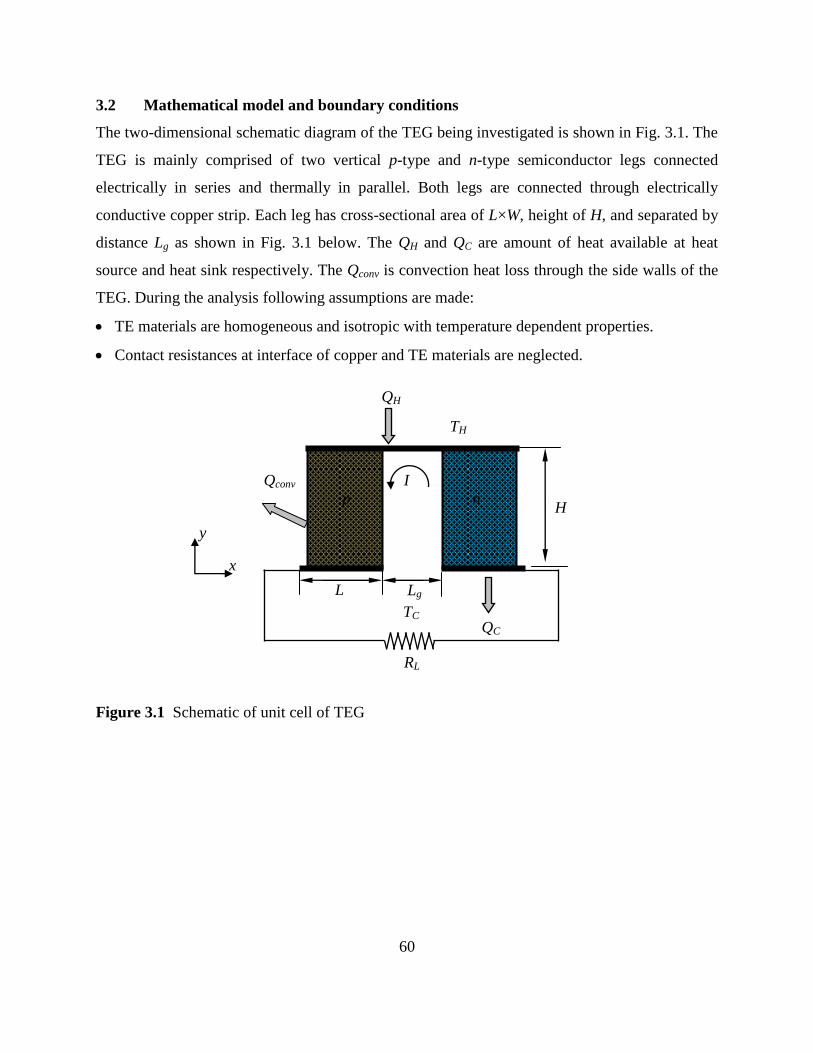
60

3.2 Mathematical model and boundary conditions

The two-dimensional schematic diagram of the TEG being investigated is shown in Fig. 3.1. The

TEG is mainly comprised of two vertical p-type and n-type semiconductor legs connected

electrically in series and thermally in parallel. Both legs are connected through electrically

conductive copper strip. Each leg has cross-sectional area of L×W, height of H, and separated by

distance Lg as shown in Fig. 3.1 below. The QH and QC are amount of heat available at heat

source and heat sink respectively. The Qconv is convection heat loss through the side walls of the

TEG. During the analysis following assumptions are made:

TE materials are homogeneous and isotropic with temperature dependent properties.

Contact resistances at interface of copper and TE materials are neglected.

Figure 3.1 Schematic of unit cell of TEG

L

p n

RL

TH

TC

I Qconv

QH

QC

H

Lg

x

y

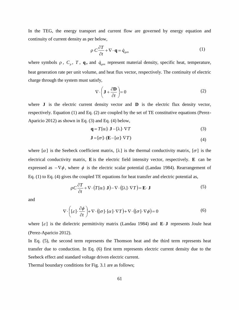
61

In the TEG, the energy transport and current flow are governed by energy equation and

continuity of current density as per below,

genqt

TC

q (1)

where symbols , pC , T , q , and genq represent material density, specific heat, temperature,

heat generation rate per unit volume, and heat flux vector, respectively. The continuity of electric

charge through the system must satisfy,

0

t

DJ (2)

where J is the electric current density vector and D is the electric flux density vector,

respectively. Equation (1) and Eq. (2) are coupled by the set of TE constitutive equations (Perez-

Aparicio 2012) as shown in Eq. (3) and Eq. (4) below,

TT ][][ Jq

)][(][ T EJ

(3)

(4)

where ][ is the Seebeck coefficient matrix, ][ is the thermal conductivity matrix, ][ is the

electrical conductivity matrix, E is the electric field intensity vector, respectively. E can be

expressed as , where is the electric scalar potential (Landau 1984). Rearrangement of

Eq. (1) to Eq. (4) gives the coupled TE equations for heat transfer and electric potential as,

JEJ

TT

t

TC ][][ (5)

and

0][][][][

Tt

(6)

where ][ is the dielectric permittivity matrix (Landau 1984) and JE represents Joule heat

(Perez-Aparicio 2012).

In Eq. (5), the second term represents the Thomson heat and the third term represents heat

transfer due to conduction. In Eq. (6) first term represents electric current density due to the

Seebeck effect and standard voltage driven electric current.

Thermal boundary conditions for Fig. 3.1 are as follows;

62

The top surface of the TEG experiences constant hot temperature (TH)

The bottom surface experiences constant cold temperature (TC)

The vertical surfaces of p type and n type are considered with two different

conditions: convective heat transfer condition and adiabatic condition (special case).


In this section, the performance of unit cell of TEG is investigated based on the results obtained

by numerically solving governing equations presented in previous section. For p-type material,

the nanostructured semiconductor Bismuth Antimony Telluride (BiSbTe) is considered to

analyze the performance (Poudel et al. 2008). While for n-type material, Bismuth Telluride

(Bi2Te3) with nano-particles of silicon carbide (SiC) is considered to analyze the performance

(Zhao et al. 2008). The temperature dependent transport parameters Seebeck coefficient )( ,

electrical conductivity )( , and thermal conductivity )( are specified as polynomial functions

of temperature as shown in Table 3.1. These properties are evaluated at an average temperature

of working temperature range. The semiconductor leg of unit cell of TEG has dimensions of

mmmm 5.15.1 and height of mm5 . The gap between two consecutive legs is mm3.0 . The

terminals of both p-type and n-type semiconductor legs are connected with external load (RL)

which is matched with total internal resistance of the TEG. Figures 3.2, 3.4, 3.6, and 3.8 show

field plots of temperature and heat flow. Temperature is presented by marked isothermal lines

with multi-colored background, while the heat flow is presented by the vertical lines with arrows.

Similarly, Figs. 3.3, 3.5, 3.7, and 3.9 present the field results of electric scalar potential and

current flow. The electric potential is indicated by the marked iso-potential lines with multi-

colored background, while the current flow is indicated by the lines with arrows. Surface to

surrounding convection heat losses are also considered from vertical walls of both semiconductor

legs (h=15-50 W/m2K).

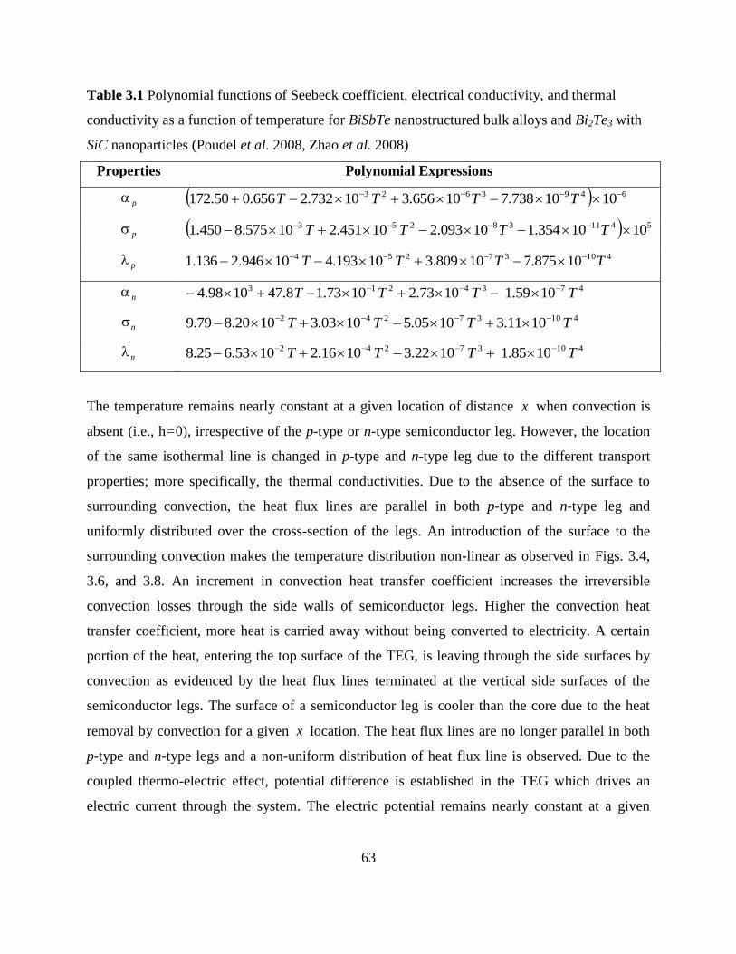
63

Table 3.1 Polynomial functions of Seebeck coefficient, electrical conductivity, and thermal

conductivity as a function of temperature for BiSbTe nanostructured bulk alloys and Bi2Te3 with

SiC nanoparticles (Poudel et al. 2008, Zhao et al. 2008)

Properties Polynomial Expressions

p 6493623 1010738.710656.310732.2656.050.172 TTTT

p 541138253 1010354.110093.210451.210575.8450.1 TTTT

p 41037254 10875.710809.310193.410946.2136.1 TTTT

n 4734213 1059.11073.21073.18.471098.4 TTTT

n 41037242 1011.31005.51003.31020.879.9 TTTT

n 41037242 1085.11022.31016.21053.625.8 TTTT

The temperature remains nearly constant at a given location of distance x when convection is

absent (i.e., h=0), irrespective of the p-type or n-type semiconductor leg. However, the location

of the same isothermal line is changed in p-type and n-type leg due to the different transport

properties; more specifically, the thermal conductivities. Due to the absence of the surface to

surrounding convection, the heat flux lines are parallel in both p-type and n-type leg and

uniformly distributed over the cross-section of the legs. An introduction of the surface to the

surrounding convection makes the temperature distribution non-linear as observed in Figs. 3.4,

3.6, and 3.8. An increment in convection heat transfer coefficient increases the irreversible

convection losses through the side walls of semiconductor legs. Higher the convection heat

transfer coefficient, more heat is carried away without being converted to electricity. A certain

portion of the heat, entering the top surface of the TEG, is leaving through the side surfaces by

convection as evidenced by the heat flux lines terminated at the vertical side surfaces of the

semiconductor legs. The surface of a semiconductor leg is cooler than the core due to the heat

removal by convection for a given x location. The heat flux lines are no longer parallel in both

p-type and n-type legs and a non-uniform distribution of heat flux line is observed. Due to the

coupled thermo-electric effect, potential difference is established in the TEG which drives an

electric current through the system. The electric potential remains nearly constant at a given

64

location of distance x when h=0 for a particular semiconductor leg. However, non-linear

electric potential distribution is observed with convective heat transfer boundary condition.

65

320 320

340

360 360

380

400 400

420

440

460

480480

500 500

320

340

360

380 380

400

420420

440

460

480

500

Figure 3.2 Contours of temperature distribution and streamlines of heat flow with adiabatic heat

transfer condition (h ≈ 0 W/m2K)

66

0.002

0.004

0.0060.006

0.008 0.008

0.01

0.012 0.012

0.014 0.014

0.016 0.016

-0.018

-0.016-0.016

-0.014-0.014

-0.012

-0.01

-0.008

-0.006-0.006

-0.004-0.004

-0.002

0

-0.0

14

-0.0

12

0.0

14

Figure 3.3 Contours of electric potential and streamlines of electric current flow with adiabatic

heat transfer condition (h ≈ 0 W/m2K)

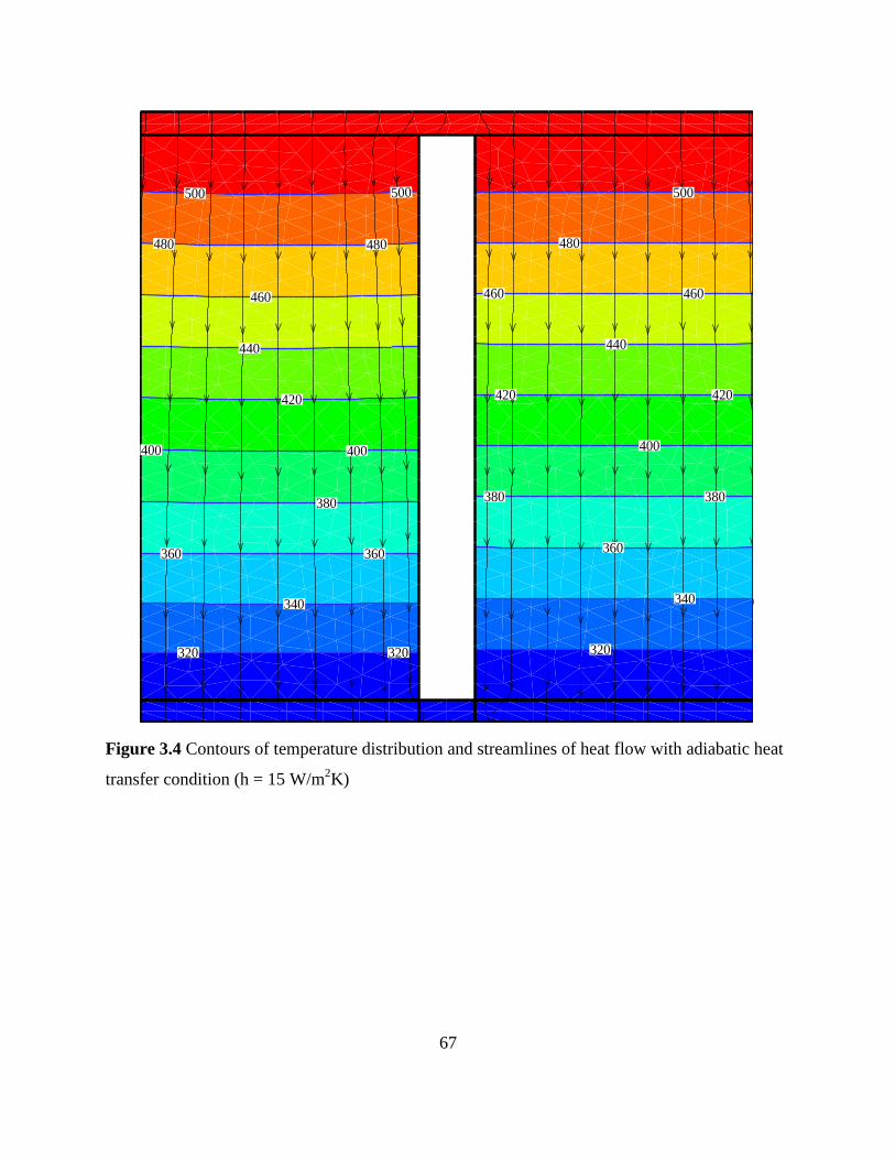
67

320 320

340

360 360

380

400 400

420

440

460

480480

500 500

320

340

360

380380

400

420420

440

460460

480

500


transfer condition (h = 15 W/m2K)

68

0.002

0.004

0.0060.006

0.008 0.008

0.01

0.012 0.012

0.014

-0.014-0.014

-0.012

-0.01

-0.008

-0.006-0.006

-0.004-0.004

-0.002

0

0.0

06 0

.01


heat transfer condition (h = 15 W/m2K)

69

320 320

340

360 360

380

400 400

420

440

460

480480

500 500

320

340

360

380380

400

420420

440

460460

480

500



70

0.002

0.004

0.0060.006

0.008

0.010.01

0.012

0.014

-0.014-0.014

-0.012

-0.01-0.01

-0.008

-0.006

-0.004

-0.002

00

-0.0

14

00.0

1



71

320 320

340

360 360

380

400 400

420

440

460

480 480

500

320

340

360

380380

400

420420

440

460

480

500



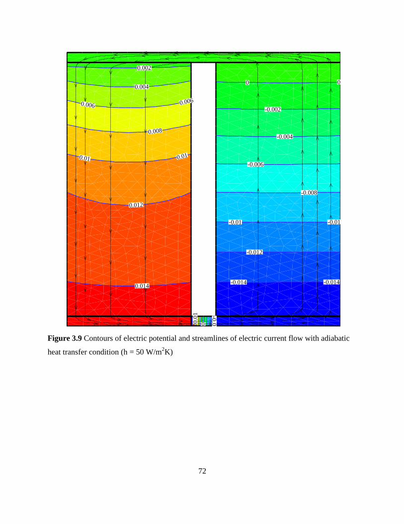
72

0.002

0.004

0.0060.006

0.008

0.010.01

0.012

0.014-0.014-0.014

-0.012

-0.01-0.01

-0.008

-0.006

-0.004

-0.002

00

-0.0

14

00.0

1



73

In addition to the numerical simulation, a comparison between analytical result and numerical

simulation is presented in terms of the current produced. The analytical results are obtained from

the mathematical model developed by Reddy et al. (2013). The comparison is presented in Fig.

3.10 where produced current is plotted as a function of temperature difference between hot and

cold surface of the TEG. The electric current increases as temperature difference increases.

Figure 3.10 establishes a good agreement between the current result and result available in the

literature. The proposed nanostructured TEG’s thermal efficiency is demonstrated in Fig. 3.11

where thermal efficiency is plotted as a function of temperature difference between hot and cold

surface of the TEG at different values of convection heat transfer coefficients. TEG has highest

efficiency with larger temperature difference and adiabatic boundary condition. As convection

heat transfer coefficient increases, the thermal efficiency drops and this can be attributed to heat

loss shown in temperature field plots from Figs. 3.4, 3.6, and 3.8.

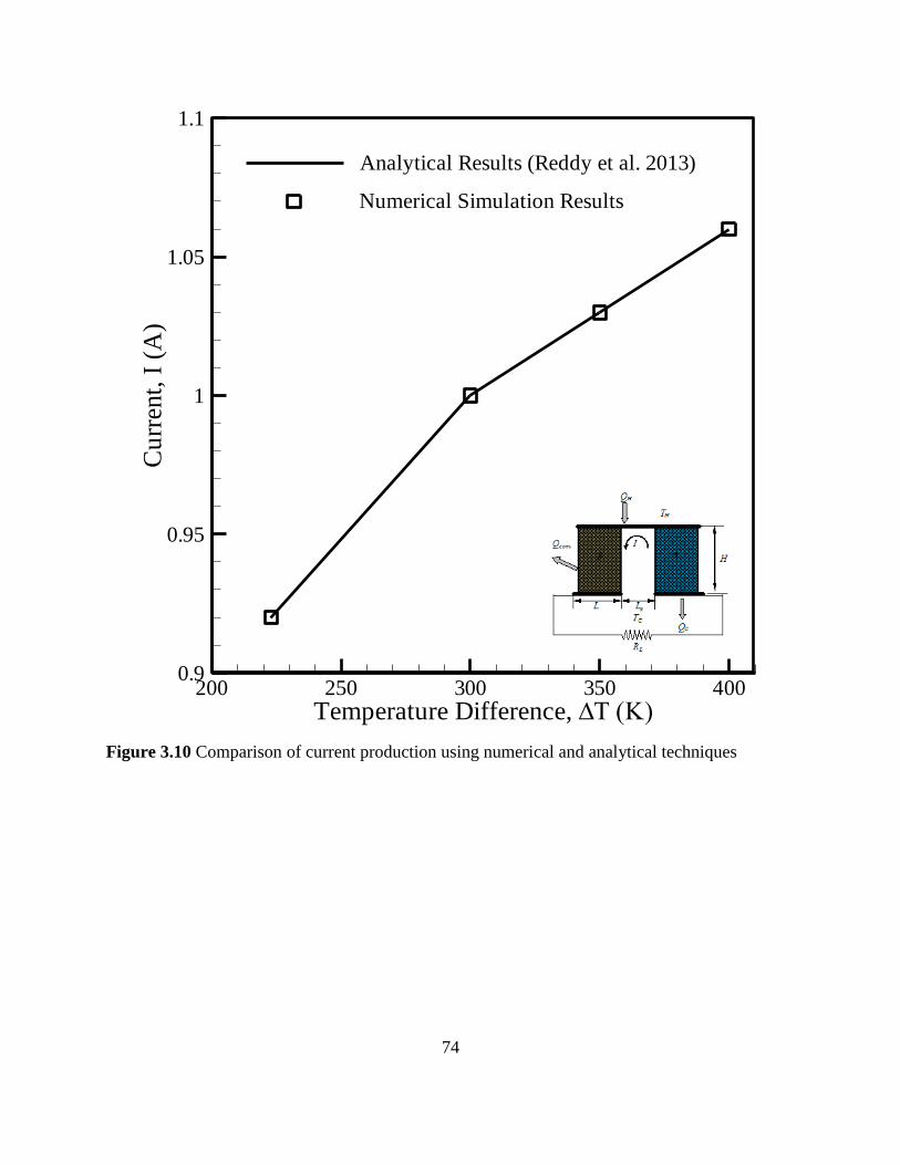
74

Temperature Difference,

Cu

rren

t,I

(A)

200 250 300 350 4000.9

0.95

1

1.05

1.1

Analytical Results (Reddy et al. 2013)

Numerical Simulation Results

Figure 3.10 Comparison of current production using numerical and analytical techniques

75

h = 15 W/m2K

Temperature Difference,

Th

erm

al

Eff

icie

ncy

,

200 250 300 350 4003.5

4

4.5

5

5.5

6

6.5

7

h = 0 W/m2K

h = 35 W/m2K

h = 50 W/m2K

Figure 3.11 Thermal efficiency of TEG as a function of convection heat transfer coefficient and

temperature difference

76

3.4 Conclusion

In this research work, a numerical simulation of nanostructured TEG is carried out. The

nanostructured TE materials have low thermal conductivity and higher power factor ( 2 )

which improves performance of the TEG. Current numerical simulation considers the Seebeck

effect, Peltier effect, Thomson effect, Fourier heat conduction, and convection heat transfer

losses. The influences of hot surface temperature and convection heat transfer coefficient on the

performance parameters of TEG such as thermal efficiency and electric current have been

studied. Electric current generation using numerical simulation and analytical simulation shows a

good match. An increase in hot surface temperature leads to increase in electric current

generation and eventually the thermal efficiency. Numerical results prove that presence of

irreversible convection heat transfer causes a large amount of heat loss thus reduces the thermal

efficiency. In future, more detailed three-dimensional numerical simulation of TEG will be

carried out to observe the above mentioned effects in more detail.

77

3.5 Nomenclature

C specific heat capacity (kJkg-1

K-1

)

D electric flux density vector (Cm-2

)


)

e electron charge (C)


K-1

)

H height of TE leg (m)

I current (A)

J electric current density vector (Am-2

)

k Boltzmann constant (JK-1

)

L length (m)

oL Lorentz number (V2K

-2)

R resistance (Ω)

q heat flux vector (Wm-2

)

.


)

Q heat (W)

t time (S)

T temperature (K)

W width of the TE leg (m)

x coordinate (m)

y coordinate (m)

ZT dimensionless figure of merit

Greek symbols


)

ε dielectric permittivity matrix (Fm-1

)

thermal conductivity (Wm-1

K-1

)

density (kgm-3

)


)


78

Subscripts

C cold surface

conv convection

E electronic

g gap

H hot surface

l external load

L lattice

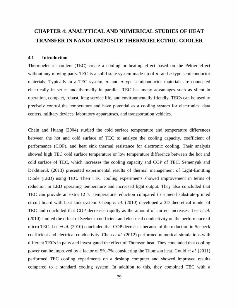
79

CHAPTER 4: ANALYTICAL AND NUMERICAL STUDIES OF HEAT

TRANSFER IN NANOCOMPOSITE THERMOELECTRIC COOLER

4.1 Introduction

Thermoelectric coolers (TEC) create a cooling or heating effect based on the Peltier effect

without any moving parts. TEC is a solid state system made up of p- and n-type semiconductor

materials. Typically in a TEC system, p- and n-type semiconductor materials are connected

electrically in series and thermally in parallel. TEC has many advantages such as silent in

operation, compact, robust, long service life, and environmentally friendly. TECs can be used to

precisely control the temperature and have potential as a cooling system for electronics, data

centers, military devices, laboratory apparatuses, and transportation vehicles.

Chein and Huang (2004) studied the cold surface temperature and temperature differences

between the hot and cold surface of TEC to analyze the cooling capacity, coefficient of

performance (COP), and heat sink thermal resistance for electronic cooling. Their analysis

showed high TEC cold surface temperature or low temperature difference between the hot and

cold surface of TEC, which increases the cooling capacity and COP of TEC. Semenyuk and

Dekhtiaruk (2013) presented experimental results of thermal management of Light-Emitting

Diode (LED) using TEC. Their TEC cooling experiments showed improvement in terms of

reduction in LED operating temperature and increased light output. They also concluded that

TEC can provide an extra 12 ºC temperature reduction compared to a metal substrate-printed

circuit board with heat sink system. Cheng et al. (2010) developed a 3D theoretical model of

TEC and concluded that COP decreases rapidly as the amount of current increases. Lee et al.

(2010) studied the effect of Seebeck coefficient and electrical conductivity on the performance of

micro TEC. Lee et al. (2010) concluded that COP decreases because of the reduction in Seebeck

coefficient and electrical conductivity. Chen et al. (2012) performed numerical simulations with

different TECs in pairs and investigated the effect of Thomson heat. They concluded that cooling

power can be improved by a factor of 5%-7% considering the Thomson heat. Gould et al. (2011)

performed TEC cooling experiments on a desktop computer and showed improved results

compared to a standard cooling system. In addition to this, they combined TEC with a

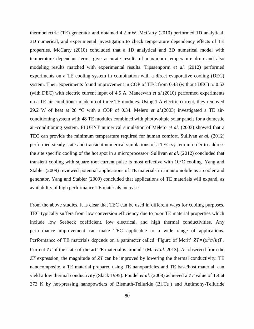
80

thermoelectric (TE) generator and obtained 4.2 mW. McCarty (2010) performed 1D analytical,

3D numerical, and experimental investigation to check temperature dependency effects of TE

properties. McCarty (2010) concluded that a 1D analytical and 3D numerical model with

temperature dependant terms give accurate results of maximum temperature drop and also

modeling results matched with experimental results. Tipsaenporm et al. (2012) performed

experiments on a TE cooling system in combination with a direct evaporative cooling (DEC)

system. Their experiments found improvement in COP of TEC from 0.43 (without DEC) to 0.52

(with DEC) with electric current input of 4.5 A. Maneewan et al.(2010) performed experiments

on a TE air-conditioner made up of three TE modules. Using 1 A electric current, they removed

29.2 W of heat at 28 °C with a COP of 0.34. Melero et al.(2003) investigated a TE air-

conditioning system with 48 TE modules combined with photovoltaic solar panels for a domestic

air-conditioning system. FLUENT numerical simulation of Melero et al. (2003) showed that a

TEC can provide the minimum temperature required for human comfort. Sullivan et al. (2012)

performed steady-state and transient numerical simulations of a TEC system in order to address

the site specific cooling of the hot spot in a microprocessor. Sullivan et al. (2012) concluded that

transient cooling with square root current pulse is most effective with 10°C cooling. Yang and

Stabler (2009) reviewed potential applications of TE materials in an automobile as a cooler and

generator. Yang and Stabler (2009) concluded that applications of TE materials will expand, as

availability of high performance TE materials increase.

From the above studies, it is clear that TEC can be used in different ways for cooling purposes.

TEC typically suffers from low conversion efficiency due to poor TE material properties which

include low Seebeck coefficient, low electrical, and high thermal conductivities. Any

performance improvement can make TEC applicable to a wide range of applications.

Performance of TE materials depends on a parameter called ‘Figure of Merit’ ZT= Tk)( 2 .

Current ZT of the state-of-the-art TE material is around 1(Ma et al. 2013). As observed from the

ZT expression, the magnitude of ZT can be improved by lowering the thermal conductivity. TE

nanocomposite, a TE material prepared using TE nanoparticles and TE base/host material, can

yield a low thermal conductivity (Slack 1995). Poudel et al. (2008) achieved a ZT value of 1.4 at

373 K by hot-pressing nanopowders of Bismuth-Telluride (Bi2Te3) and Antimony-Telluride

81

(Sb2Te3) under Argon (Ar) atmosphere. The enhanced ZT was due to the significant reduction in

the thermal conductivity of material (Poudel 2008). Fan et al. (2011) prepared a n-type Bi2Te3

nanocomposite which exhibited a ZT of 1.18 due to reduction in thermal conductivity. Tang et

al.(2011) prepared double- filled Cobalt Triantimonide (CoSb3) using Indium (In) and Lutetium

(Lu) resulting into In0.13Lu0.05Co4.02Sb12 through a high-pressure synthesis method.

In0.13Lu0.05Co4.02Sb12 yielded a ZT of 0.27 which was greater by one order of magnitude than that

of CoSb3 (Tang el al. 2011). Nagami et al. (2014) prepared a Bismuth-Antimony-Telluride

(Bi0.4Sb1.6Te3) bulk TE material using mechanical alloying and hot extrusion. Their material

exhibited a ZT of 1.2 due to high electrical and low thermal conductivity.

Nanocomposite TE materials have the potential to be used as a viable tool for cooling system in

future. In order to study a nanostructured TE generator, Rabari et al. (2014) performed 2D

numerical simulations of a nanostructured TE generator and concluded that convection heat

transfer from side surfaces of a TE generator lowers the efficiency. It is also very important to

investigate the effects of convection heat transfer on the performance of a nanocomposite TEC

which is very limited in the current literature. In this work, an analytical heat transfer model of a

nanocomposite TEC is derived. All TE effects (Seebeck, Peltier, and Thomson effect), heat

conduction, and convection heat transfer are included in both analytical modeling and numerical

simulations. Analytical results are presented with different electric currents, cold surface

temperatures, and convection heat transfer coefficients. The field plots of heat and temperature

distributions are presented with different convection heat transfer coefficients. Numerical results

are compared with that of 1D analytical results in terms of heat absorbed and COP. The structure

of the work is in the following order: derivation of an analytical model, results and discussions

on analytical model, and field plots of numerical simulations.

4.2 Modeling

Figure 4.1 shows a 2D schematic diagram of the nanocomposite TEC considered in this work. A

unit cell of a TEC is made-up of one p-type and one n-type leg of semiconductor materials

connected electrically in series and thermally in parallel. An electrically conductive copper strip

connects both semiconductor legs. Materials we have considered for the current analyses are

82

nanostructured p-type Bi0.5Sb1.5Te3 (Poudel et al. 2008) and n-type Bi2Te3

(Fan et al. 2011).

Figures 4.2 and 4.3 show crystal structures of Bi0.5Sb1.5Te3 and Bi2Te3 (Zhang et al. 2011, Chen

et al. 2009). Both materials possess the tetradymite type crystal structure formed by quintuple

layers made up of 2 sheets of Bi and 3 sheets of Te (Zhang et al. 2011). For Bi0.5Sb1.5Te3, Bi

atoms are substituted by Sb (Chen et al. 2009). P-type Bi0.5Sb1.5Te3

(Poudel et al. 2008) and n-

type Bi2Te3 (Fan et al. 2011) were prepared by hot pressing the nano-powder of materials. P-type

Bi0.5Sb1.5Te3 was prepared via direct current hot press method using nanopowders of

Bi0.5Sb1.5Te3 which was prepared from ball milling of Bi0.5Sb1.5Te3 alloy ingots (Poudel et al.

2008). Nanopowders of p-type Bi0.5Sb1.5Te3 had an average size of 20 nm (Poudel et al. 2008).

The microstructure of the p-type nanostructured Bi0.5Sb1.5Te3 shows highly crystalline structure

and nanosize grains as observed from the Scanning Electron Microscope (SEM) images available

in Poudel et al. (2008). The n-type Bi2Te3 was prepared by melt spinning and hot pressing

different amounts of nanoparticles of Bi2Te3 (Fan et al. 2011). The microstructure of the

nanostructured n-type Bi2Te3 possesses a wire like structure with a mixture of micron and nano

size particles as observed from the SEM images available in Fan et al. (2011).

Figure 4.1 Schematic diagram of unit cell of TEC (drawing is not to scale)

n

W

p

TC

TH

I

Qab

Qre

L

Wg

x

Qc

83

As shown in Fig. 4.1 each semiconductor leg has a height of L, a cross-sectional area of D×W,

and the two legs are separated by a distance of Wg. TEC absorbs Qab amount of heat from the

system and rejects Qre amount of heat to the surroundings. There is also a convection heat

transfer (Qc) through the side walls of the TEC. For the analysis, the following assumptions are

made:

TE nanocomposite materials are homogeneous and isotropic.

Contact resistances at interface of copper and TE materials are neglected.

Energy transport and current flow in nanocomposite TEC considering steady state system can be

expressed as

gen

.q q (1)

0 J (2)

where q ,gen

.q , and J are heat flux, heat generation rate per unit volume, and electric current

density, respectively.

Figure 4.2 The schematic of crystal structure of (a) (Bi1-xSbx)2Te3 (Zhang et al. 2011) Reprinted

by permission from Macmillan Publishers Ltd: Nature Communications from Zhang et al. 2, 574

(2011), copyright 2011

One

quintuple

layer




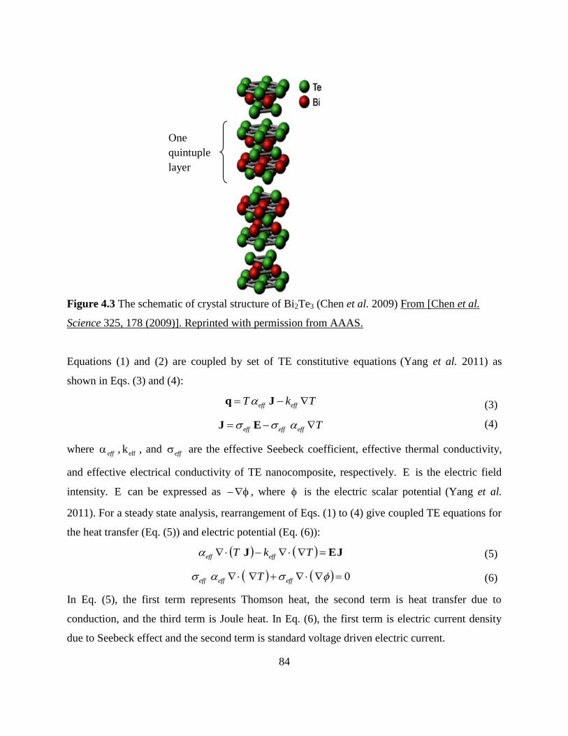
84

Figure 4.3 The schematic of crystal structure of Bi2Te3 (Chen et al. 2009) From [Chen et al.

Science 325, 178 (2009)]. Reprinted with permission from AAAS.

Equations (1) and (2) are coupled by set of TE constitutive equations (Yang et al. 2011) as

shown in Eqs. (3) and (4):

TkT effeff Jq

Teffeffeff EJ

(3)

(4)

where eff , effk , and eff are the effective Seebeck coefficient, effective thermal conductivity,

and effective electrical conductivity of TE nanocomposite, respectively. E is the electric field

intensity. E can be expressed as , where is the electric scalar potential (Yang et al.

2011). For a steady state analysis, rearrangement of Eqs. (1) to (4) give coupled TE equations for

the heat transfer (Eq. (5)) and electric potential (Eq. (6)):

JEJ TkT effeff (5)

0 effeffeff T (6)

In Eq. (5), the first term represents Thomson heat, the second term is heat transfer due to

conduction, and the third term is Joule heat. In Eq. (6), the first term is electric current density

due to Seebeck effect and the second term is standard voltage driven electric current.

One

quintuple

layer



85

In order to analyze a nanocomposite TEC analytically, Eq. (5) is simplified to obtain 1D form as

shown in Eq. (7) below and solved.

0)(

heat Thomsonferheat trans Convectionheat Joule

2

2

conductionheatFourier

2

2

dx

dT

Ak

ITT

Ak

ph

Ak

I

dx

Td

eff

a

effeff

eff

(7)

Solution of Eq. (7) in terms of temperature distribution using boundary conditions; (x = 0, T =

TC; x = L, T = TH) is given by

)(

)()(12

112221

LCLC

LC

C

LC

H

xCLC

C

LC

H

xC

ee

eTeTeeTeTexT (8)

Different terms used in Eq. (8) can be defined as

2

42

1

C ;

2

42

2

C

;Ak

I

eff

;

Ak

ph

eff

2

2

Ak

IT

Ak

ph

eff

eff

a

eff

.

(9)

(10)

Heat absorbed at the cold surface of a TEC can be written by combining Peltier heat which

occurs at junctions only

)(

)()(12

112221

21

LCLC

LC

C

LC

H

xCLC

C

LC

H

xC

eff

Ceffab

ee

eTeTeCeTeTeCAk

TIQ

(11)

An electric power input to TEC is given by

iRIP 2 (12)

where Ri can be calculated by

n

nneff,

p

ppeff,

A

L

A

LRi

(13)

Moreover, Seebeck coefficient and thermal conductivity of unit cell of a TE system can be

calculated by

n

nneff,

p

ppeff,

L

Ak

L

AkK (14)

neffpeff ,, (15)

86

To measure the performance of a TEC, the COP can be written as

COPP

Qab (16)

It is important to note that Eq. (11) is the heat absorbed by one TE leg only. Heat absorbed by

unit cell of a TEC as shown in Figure 4.1 can be calculated by considering respective properties

of both p- and n-type TE legs.

4.3 Results and discussions

In this section, the performance of a unit cell of TEC is presented based on results obtained by

analytical modeling and numerical simulations based on modeling section. For p-type material, a

nanostructured semiconductor BiSbTe is considered to analyze the performance (Poudel et al.

2008). while for n-type material nanocomposite Bi2Te3 is considered to analyze the performance

(Fan et al. 2011). The temperature dependent transport properties of nanocomposite and

conventional TE materials such as the Seebeck coefficient, electrical conductivity, and thermal

conductivity are specified as polynomial functions of temperature as shown in Table 4.1 and 4.2.

These properties are evaluated at an average temperature of a working temperature range. Two

different cases of cold surface temperatures (TC) = 333 K and (TC) = 343 K are considered with

hot surface temperature (TH) = 353 K. It is assumed that proposed TEC is used in cooling data

center processors which has a temperature limit of 85 ºC

(Ebrahimi et al. 2014). A

semiconductor leg of a unit cell of TEC has a width and thickness (W×D) of 2 mm × 2 mm and a

height (L) of 5 mm. The gap between two consecutive legs (Wg) is 0.5 mm.

87


conductivity as a function of temperature for BiSbTe nanostructured bulk alloys and

nanocomposite Bi2Te3 (Poudel et al. 2008, Fan et al. 2011)

TE

Properties

Polynomial Expressions

)p(eff 6493623 10)10738.710656.310732.2656.050.172( TTTT

)p(eff 541138253 10)10354.110093.210451.210575.8450.1( TTTT

)p(effk 41037254 10875.710809.310193.410946.2136.1 TTTT

)n(eff

648

362312

10)10246.1

10003.51043.110884.21035.1(

T

TTT

)n(eff 34936232 10)10075.710907.110815.1003.11024.2( TTTT

)n(effk 41037254 T10079.4T10991.1T10696.1T10907.1035.1


conductivity as a function of temperature for BiSbTe bulk alloys and conventional Bi2Te3

(Poudel et al. 2008, Fan et al. 2011)

TE

Properties

Polynomial Expressions

p 6483524 10)10281.210497.110637.9504.090.201( TTTT

p 541138253 10)10323.910165.810464.310053.8165.1( TTTT

pk 4937253 T10009.1T10477.4T10920.2T10023.1415.1

n 64734222 10)1033.21020.11015.262.11004.1( TTTT

n 34936232 10)1062.81025.71057.315.11036.2( TTTT

nk 41037253 T1076.1T1059.1T1025.6T1021.531.1

88

Analytical results

This section presents analytical results of a nanocomposite TEC. A temperature distribution

across a TE leg is plotted with adiabatic and convective boundary conditions. The heat absorbed

and COP of a TEC are also plotted and discussed as functions of convection heat transfer

coefficients, electric current inputs, and temperature differences. At the end of this section, the

maximum heat absorption and COP results are plotted with an optimum electric current,

convection heat transfer coefficients and TE leg heights.

Figures 4.4 and 4.5 show temperature distribution over the length of a TE leg with convection

heat transfer coefficients from 10-7

Wm-2

K-1

(adiabatic) to 80 Wm-2

K-1

. The surrounding

temperature is considered to be an average working range of hot and cold surface temperatures.

Temperature distribution remains distinct for p- and n-type leg because of their different TE

properties. P-type leg exhibits more Joule heat generation compared to n-type leg which can be

observed by temperature profile with an adiabatic side wall condition in Figs. 4.4 and 4.5. This

can be attributed to high electrical resistivity of p-type material compared to n-type material as

shown in Fig. 4.6.

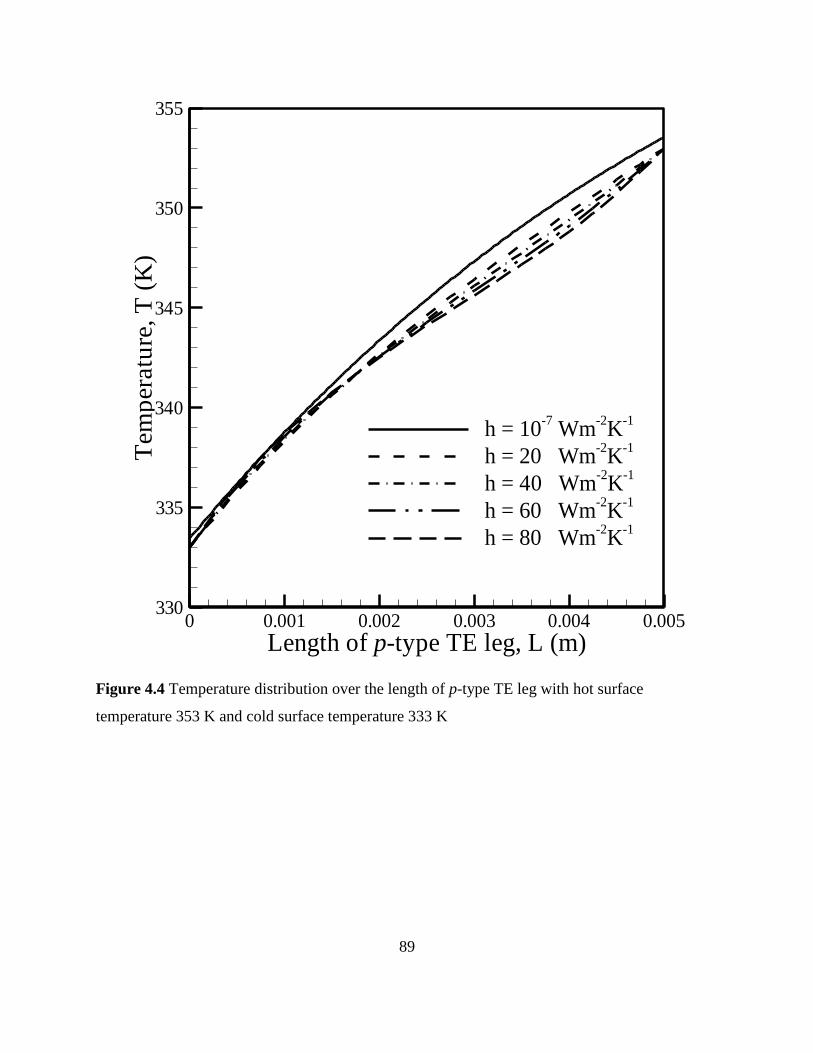
89

Length of p-type TE leg, L (m)

Tem

per

atu

re,

T(K

)

0 0.001 0.002 0.003 0.004 0.005330

335

340

345

350

355

h = 10-7

Wm-2

K-1

h = 20 Wm-2

K-1

h = 40 Wm-2

K-1

h = 60 Wm-2

K-1

h = 80 Wm-2

K-1

Figure 4.4 Temperature distribution over the length of p-type TE leg with hot surface


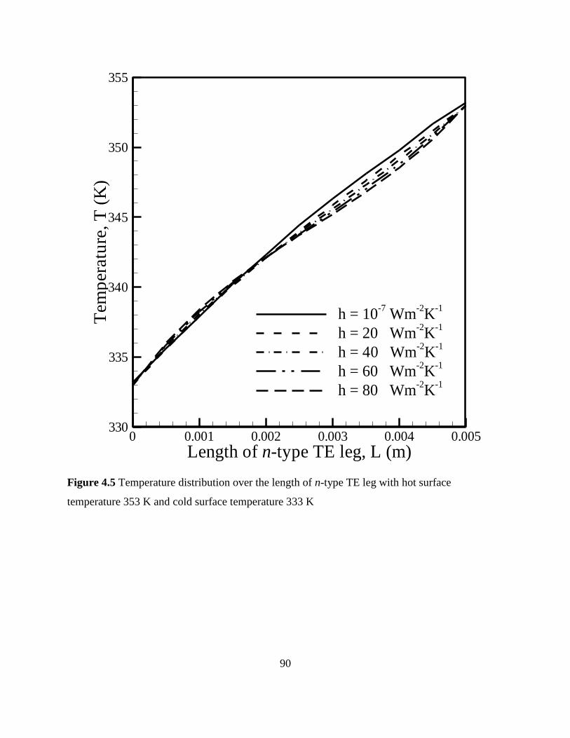
90

Length of n-type TE leg, L (m)

Tem

per

atu

re,

T(K

)

0 0.001 0.002 0.003 0.004 0.005330

335

340

345

350

355

h = 10-7

Wm-2

K-1

h = 20 Wm-2

K-1

h = 40 Wm-2K

-1

h = 60 Wm-2

K-1

h = 80 Wm-2

K-1

Figure 4.5 Temperature distribution over the length of n-type TE leg with hot surface


91

n-type material

Temperature, T (C)

Eff

ecti

ve

ele

ctr

ical

resi

stiv

ity

,

eff

(m

)

0 50 100 150 200 2500

5E-06

1E-05

1.5E-05

2E-05

2.5E-05

p-type material

Figure 4.6 Electrical resistivity of p- and n- type legs of nanocomposite TEC

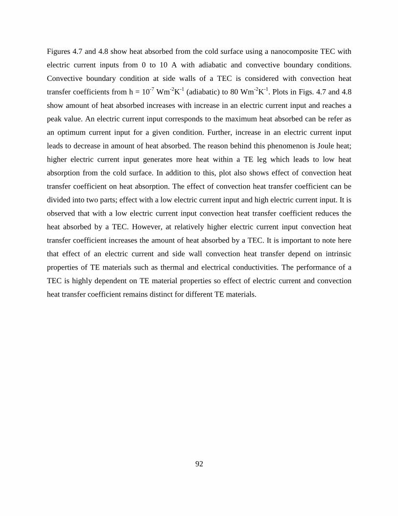
92

Figures 4.7 and 4.8 show heat absorbed from the cold surface using a nanocomposite TEC with

electric current inputs from 0 to 10 A with adiabatic and convective boundary conditions.

Convective boundary condition at side walls of a TEC is considered with convection heat

transfer coefficients from h = 10-7

Wm-2

K-1

(adiabatic) to 80 Wm-2

K-1

. Plots in Figs. 4.7 and 4.8

show amount of heat absorbed increases with increase in an electric current input and reaches a

peak value. An electric current input corresponds to the maximum heat absorbed can be refer as

an optimum current input for a given condition. Further, increase in an electric current input

leads to decrease in amount of heat absorbed. The reason behind this phenomenon is Joule heat;

higher electric current input generates more heat within a TE leg which leads to low heat

absorption from the cold surface. In addition to this, plot also shows effect of convection heat

transfer coefficient on heat absorption. The effect of convection heat transfer coefficient can be

divided into two parts; effect with a low electric current input and high electric current input. It is

observed that with a low electric current input convection heat transfer coefficient reduces the

heat absorbed by a TEC. However, at relatively higher electric current input convection heat

transfer coefficient increases the amount of heat absorbed by a TEC. It is important to note here

that effect of an electric current and side wall convection heat transfer depend on intrinsic

properties of TE materials such as thermal and electrical conductivities. The performance of a

TEC is highly dependent on TE material properties so effect of electric current and convection

heat transfer coefficient remains distinct for different TE materials.

93

Current, I (A)

Hea

tab

sorb

ed,

Qab

(W)

2 4 6 8 100

0.1

0.2

0.3

0.4

0.5

h = 10-7

Wm-2

K-1

h = 20 Wm-2

K-1

h = 40 Wm-2

K-1

h = 60 Wm-2

K-1

h = 80 Wm-2

K-1

Figure 4.7 Heat absorbed as a function of current considering hot surface temperature 353 K

with cold surface temperature 333 K

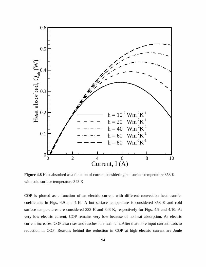
94

Current, I (A)

Hea

tab

sorb

ed,

Qab

(W)

0 2 4 6 8 100

0.1

0.2

0.3

0.4

0.5

0.6

h = 10-7

Wm-2K

-1

h = 20 Wm-2K

-1

h = 40 Wm-2

K-1

h = 60 Wm-2K

-1

h = 80 Wm-2K

-1

Figure 4.8 Heat absorbed as a function of current considering hot surface temperature 353 K


COP is plotted as a function of an electric current with different convection heat transfer

coefficients in Figs. 4.9 and 4.10. A hot surface temperature is considered 353 K and cold

surface temperatures are considered 333 K and 343 K, respectively for Figs. 4.9 and 4.10. At

very low electric current, COP remains very low because of no heat absorption. As electric

current increases, COP also rises and reaches its maximum. After that more input current leads to

reduction in COP. Reasons behind the reduction in COP at high electric current are Joule

95

heating, increase in power input, and relatively low improvement in the heat absorption. The

same plot, also investigates the effect of convection heat transfer coefficient. Effect of

convection heat transfer coefficient can be divided into two distinct categories same as heat

absorption. For relatively low electric current input, COP decreases as convection heat transfer

coefficient increases. In contrary, COP increases with an increase in convection heat transfer

coefficient with relatively high electric current input. The reason behind relatively higher COP at

higher convection heat transfer coefficient is heat transfer through side walls of TE legs with

surroundings which help escapes the higher amount of Joule heat and absorbed heat.

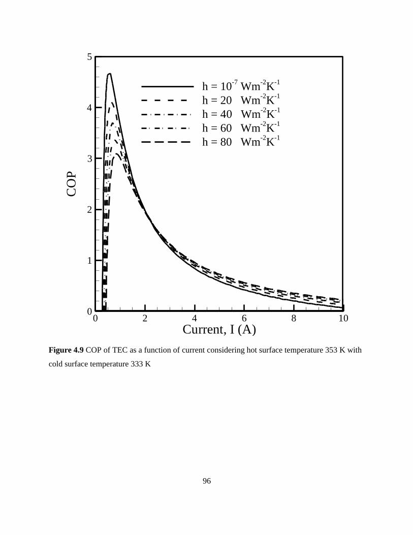
96

Current, I (A)

CO

P

0 2 4 6 8 100

1

2

3

4

5

h = 10-7

Wm-2

K-1

h = 20 Wm-2

K-1

h = 40 Wm-2

K-1

h = 60 Wm-2

K-1

h = 80 Wm-2

K-1

Figure 4.9 COP of TEC as a function of current considering hot surface temperature 353 K with

cold surface temperature 333 K

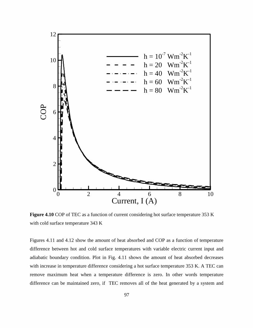
97

Current, I (A)

CO

P

0 2 4 6 8 100

2

4

6

8

10

12

h = 10-7

Wm-2

K-1

h = 20 Wm-2

K-1

h = 40 Wm-2

K-1

h = 60 Wm-2

K-1

h = 80 Wm-2

K-1

Figure 4.10 COP of TEC as a function of current considering hot surface temperature 353 K


Figures 4.11 and 4.12 show the amount of heat absorbed and COP as a function of temperature

difference between hot and cold surface temperatures with variable electric current input and

adiabatic boundary condition. Plot in Fig. 4.11 shows the amount of heat absorbed decreases

with increase in temperature difference considering a hot surface temperature 353 K. A TEC can

remove maximum heat when a temperature difference is zero. In other words temperature

difference can be maintained zero, if TEC removes all of the heat generated by a system and

98

maintains the hot surface temperature (TH) = cold surface temperature (TC). Additionally, plot

also demonstrates that higher amount of an electric current help absorb more heat but amount of

heat absorption decreases with increase in an electric current due to Joule heat. Plot in Fig. 4.12

shows variation in COP as temperature difference increases with a hot surface temperature 353 K

and adiabatic side wall condition. With variable electric current input, one can conclude that

higher amount of an electric current leads to low COP. The reason behind low COP at higher

electric current is relatively low amount of heat absorbed in comparison to power input. Also,

COP remains highest when temperature difference is zero irrespective of electric current input.

99

Temperature difference,

Hea

tab

sorb

ed,

Qab

(W)

0 5 10 15 200

0.1

0.2

0.3

0.4

0.5

I = 1 A

I = 2 A

I = 3 A

I = 4 A

I = 5 A

Figure 4.11 Heat absorbed as a function of temperature difference with different electric current

input and hot surface temperature 353 K considering adiabatic side wall condition

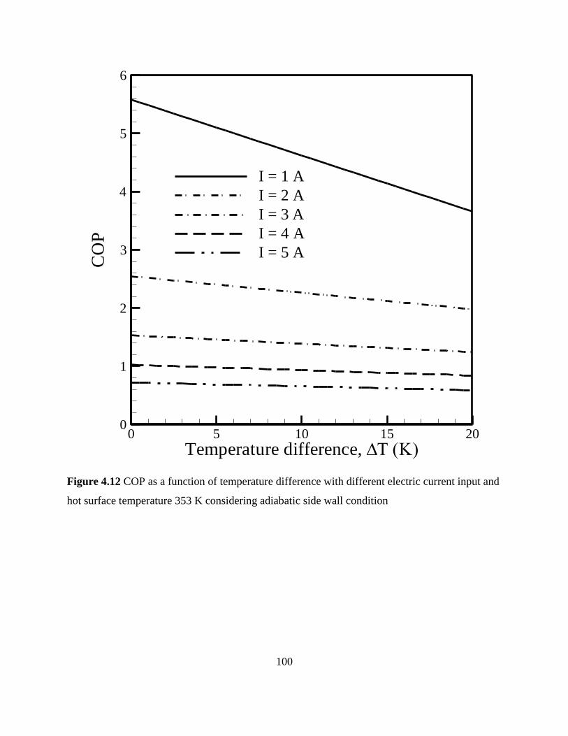
100


CO

P

0 5 10 15 200

1

2

3

4

5

6

I = 1 A

I = 2 A

I = 3 A

I = 4 A

I = 5 A

Figure 4.12 COP as a function of temperature difference with different electric current input and

hot surface temperature 353 K considering adiabatic side wall condition

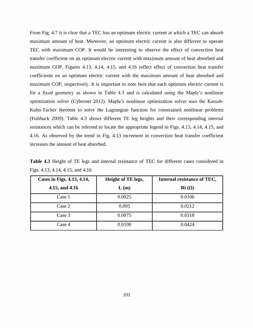
101

From Fig. 4.7 it is clear that a TEC has an optimum electric current at which a TEC can absorb

maximum amount of heat. Moreover, an optimum electric current is also different to operate

TEC with maximum COP. It would be interesting to observe the effect of convection heat

transfer coefficient on an optimum electric current with maximum amount of heat absorbed and

maximum COP. Figures 4.13, 4.14, 4.15, and 4.16 reflect effect of convection heat transfer

coefficients on an optimum electric current with the maximum amount of heat absorbed and

maximum COP, respectively. It is important to note here that each optimum electric current is

for a fixed geometry as shown in Table 4.3 and is calculated using the Maple’s nonlinear

optimization solver (Cybernet 2012). Maple’s nonlinear optimization solver uses the Karush-

Kuhn-Tucker theorem to solve the Lagrangian function for constrained nonlinear problems

(Fishback 2009). Table 4.3 shows different TE leg heights and their corresponding internal

resistances which can be referred to locate the appropriate legend in Figs. 4.13, 4.14, 4.15, and

4.16. As observed by the trend in Fig. 4.13 increment in convection heat transfer coefficient

increases the amount of heat absorbed.

Table 4.3 Height of TE legs and internal resistance of TEC for different cases considered in

Figs. 4.13, 4.14, 4.15, and 4.16

Cases in Figs. 4.13, 4.14,

4.15, and 4.16

Height of TE legs,

L (m)

Internal resistance of TEC,

Ri (Ω)

Case 1 0.0025 0.0106

Case 2 0.005 0.0212

Case 3 0.0075 0.0318

Case 4 0.0100 0.0424

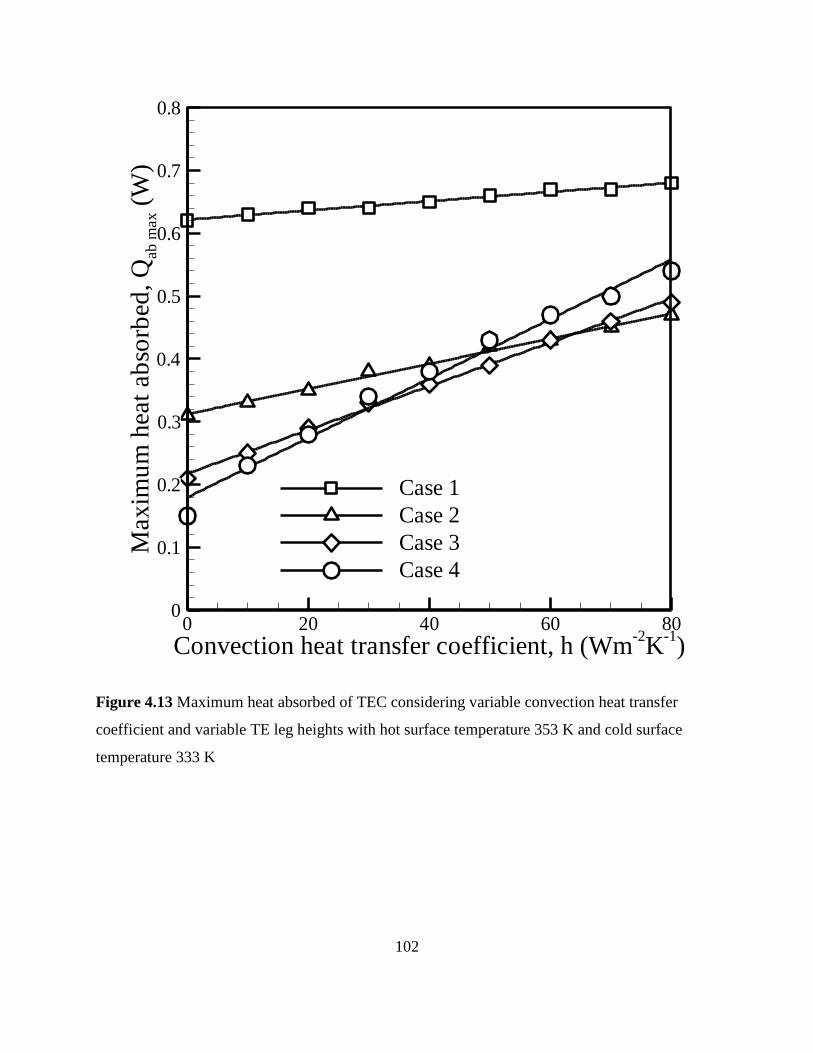
102

Convection heat transfer coefficient, h (Wm-2

K-1)

Max

imu

mh

eat

ab

sorb

ed,

Qab

max

(W)

0 20 40 60 800

0.1

0.2

0.3

0.4

0.5

0.6

0.7

0.8

Case 1

Case 2

Case 3

Case 4

Figure 4.13 Maximum heat absorbed of TEC considering variable convection heat transfer

coefficient and variable TE leg heights with hot surface temperature 353 K and cold surface

temperature 333 K

103

With adiabatic side wall conditions, the smallest TEC and longest TEC in height show maximum

and minimum heat absorption, respectively. The reason behind this is change in internal

resistance of a nanocomposite TEC as shown in Table 4.3. The smallest TEC has lowest internal

resistance which generates low Joule heat whereas longest TEC has a highest internal resistance

which generates high Joule heat. It is also clear that TEC’s optimum electric current requirement

increases with increase in a convection heat transfer coefficient. Effect of convection heat

transfer coefficient on COP can be analysed from Fig. 4.15, where COP follows decreasing trend

as convection heat transfer coefficient increases. The same plot also strengthens previous result

of higher optimum current with increment in convection heat transfer coefficient. A TEC’s

requirement of higher optimum electric current with increase in convection heat transfer

coefficient can be verified from Figs. 4.14 and 4.16. Moreover, plot also reveals that maximum

COP of a TEC is independent of height of TE legs and this same phenomenon can also verified

from Fig. 12 of Hodes (2007). Figures 4.14 and 4.16 also show that optimum electric current

remains different for maximum heat absorption and maximum COP.

104


K-1)

Op

tim

um

elec

tric

cu

rren

t,I o

pt(A

)

0 20 40 60 800

2

4

6

8

10

12

14

16

Case 1

Case 2

Case 3

Case 4

Figure 4.14 Optimum electric current for maximum heat absorption of TEC considering variable

convection heat transfer coefficient and variable TE leg heights with hot surface temperature


105


K-1)

CO

Pm

ax

0 20 40 60 800

1

2

3

4

5

Case 1

Case 2

Case 3

Case 4

Figure 4.15 Maximum COP of TEC considering variable convection heat transfer coefficient

and variable TE leg heights with hot surface temperature 353 K and cold surface temperature

333 K

106


K-1)

Op

tim

um

elec

tric

cu

rren

t,I o

pt(A

)

0 20 40 60 800

0.2

0.4

0.6

0.8

1

1.2

1.4

Case 1

Case 2

Case 3

Case 4

Figure 4.16 Optimum electric current for maximum COP of TEC considering variable

convection heat transfer coefficient and variable TE leg heights with hot surface temperature


107

Additionally, internal resistance and maximum heat absorption are plotted as a function of TE

leg height. Plots in Figs.4.17 and 4.18 show performance of a unit cell of TEC as height of TE

leg vary. As seen in Fig. 4.17, an increase in internal resistance of a unit cell of TEC is consistent

with rise in height of TE leg which is quite evident from Eq. (13) as well. The rise in internal

resistance of TEC leads to the reduction in maximum amount of heat absorbed by TEC as shown

in Fig. 4.18.

108

Height of TE leg, L(m)

Inte

rnal

Res

ista

nce,

R(

)

0 0.005 0.01 0.015 0.020

0.02

0.04

0.06

0.08

0.1

Figure 4.17 Internal resistance of TEC unit cell as a function of TE leg height

109

Height of TE leg, L(m)

Max

imu

mh

eat

ab

sorb

ed,

Qab

max

(W)

0 0.005 0.01 0.015 0.020

0.2

0.4

0.6

0.8

1

1.2

Figure 4.18 Maximum heat absorbed as a function of TE leg height by unit cell of TEC with hot

surface temperature 353 K, cold surface temperature 333 K, and adiabatic side wall condition

110

Numerical Simulation Results and Comparison

In this section, results achieved using numerical simulation is presented. Initially, the results

obtained are expressed using field plots of temperature contours with heat flow and later results

are expressed graphically. A nanocomposite TEC with width (W = 2 mm) and height (L = 5 mm)

is considered for analysis. Figures 4.19 to 4.26 present field plots of an electric potential,

temperature distribution, and heat flow with a cold surface temperature 333 K and a hot surface

temperature 353 K. Figures 4.19 and 4.20 show field results of an electric potential and electric

current flow streamlines. The terminal of TEC is applied with electric potentials of 0.02 V and

0.06 V for Figs. 4.19 and 4.20, respectively. An electric potential of 0.02 V and 0.06 V

corresponds to low and high electrical current inputs, respectively. An electric potential is

indicated by marked iso-potential lines with a multi-colored background, while current flow is

indicated by lines with arrows. Figures 4.21, 4.22, 4.23 and 4.24 show field plots of temperature

and heat flow with an electric potential of 0.02 V. At the end, Figs. 4.25 and 4.26 show field

plots of temperature and heat flow with an electric potential of 0.06 V to demonstrate Joule

heating. Temperature is presented by marked isothermal lines with multi-colored background,

while heat flow is presented by vertical lines with arrows. Vertical walls of semiconductor legs

are considered under different convective heat transfer conditions from h ≈ 0 Wm-2

K-1

to h = 60

Wm-2

K-1

. The surrounding temperature is considered to be an average temperature of a working

range. Figures 4.19 and 4.20 show distribution of an electric potential and flow of electric

current. Field plot shows electric potential distribution and current flow according to applied

electric boundary condition.

111

0.001

0.002

0.003

0.004

0.005

0.006

0.007

0.008

0.009

0.01

0.011

0.012

0.013

0.014

0.015

0.016

0.017

0.018

0.019

Figure 4.19 Electric scalar potential and current flow in nanocomposite TEC with electric

potential 0.02 V

112

0.005

0.01

0.015

0.02

0.025

0.03

0.035

0.04

0.045

0.05

0.055

Figure 4.20 Electric scalar potential and current flow in nanocomposite TEC with electric

potential 0.06 V

113

Figures 4.21, 4.22, 4.23 and 4.24 present heat flow and temperature distribution inside a

nanocomposite TEC with an electric potential 0.02 V. A nanocomposite TEC is under different

convection boundary conditions at vertical walls of semiconductor legs ranging from h ≈ 0

Wm-2

K-1

(adiabatic) to h = 60 Wm-2

K-1

. When vertical walls of semiconductor legs are adiabatic,

temperature remains nearly constant at a given location of a distance x. This remains true for

both p- and n-type semiconductor legs. Though, different thermal conductivities change the

location of the same isothermal line in p- and n-type leg. Due to the adiabatic side wall

condition, both p- and n-type legs have parallel heat flux lines with uniform distribution over the

cross-section of legs. The temperature distribution non-linearity increases as surface to the

surrounding convection heat transfer coefficient increases from h = 20 Wm-2

K-1

to h = 60

Wm-2

K-1

as observed in Figs. 4.22, 4.23, and 4.24. An introduction of a convective heat transfer

boundary condition to side walls brings heat from the surrounding because part of the

semiconductor leg is cooler than the surrounding. Higher the convection heat transfer coefficient,

more heat is being brought inside TE leg. This phenomenon reduces amount of heat absorbed

from cold surface of the TEC when low electric potential is applied.

114

334

336

338

340

342

344

346

348

350

352

334

336

338

340

342

344

346

348

350

352

Figure 4.21 Heat flow and temperature distribution in nanocomposite TEC for h ≈ 0 Wm-2

K-1

at

vertical walls with electric potential 0.02 V

115

334

336

338

340

342

344

346

348

350

352

334

336

338

340

342

344

346

348

350

352

Figure 4.22 Heat flow and temperature distribution in nanocomposite TEC for h = 20 Wm-2

K-1


116

334

336

338

340

342

344

346

348

350

352

334

336

338

340

342

344

346

348

350

352


K-1


117

334

336

338

340

342

344

346

348

350

352

334

336

338

340

342

344

346

348

350

352


K-1


118

Figures 4.25 and 4.26 present streamlines and contours of heat flow and temperature distribution

with a higher electric potential of 0.06 V. Due to higher electric potential, nanocomposite TEC

draws more current which eventually generates more Joule heat as one can see from Figs. 4.25

and 4.26. Nonetheless, this Joule heat keeps TE leg at a higher temperature compared to

surroundings which eventually transfers the heat to the surroundings from side surfaces as well.

A difference in the location of heat streamlines in Figs. 4.25 and 4.26 show that higher

temperature inside the TE leg (Fig. 4.26) transfers the heat to surroundings. Ultimately, this

phenomenon drags more heat from the cold surface of TEC.

119

334334

338

342

346

350350

354

354354

334

338 338

342 342

346346

350

Figure 4.25 Heat flow and temperature distribution in nanocomposite TEC for h ≈ 0 Wm-2

K-1

at

vertical walls with electric potential 0.06 V

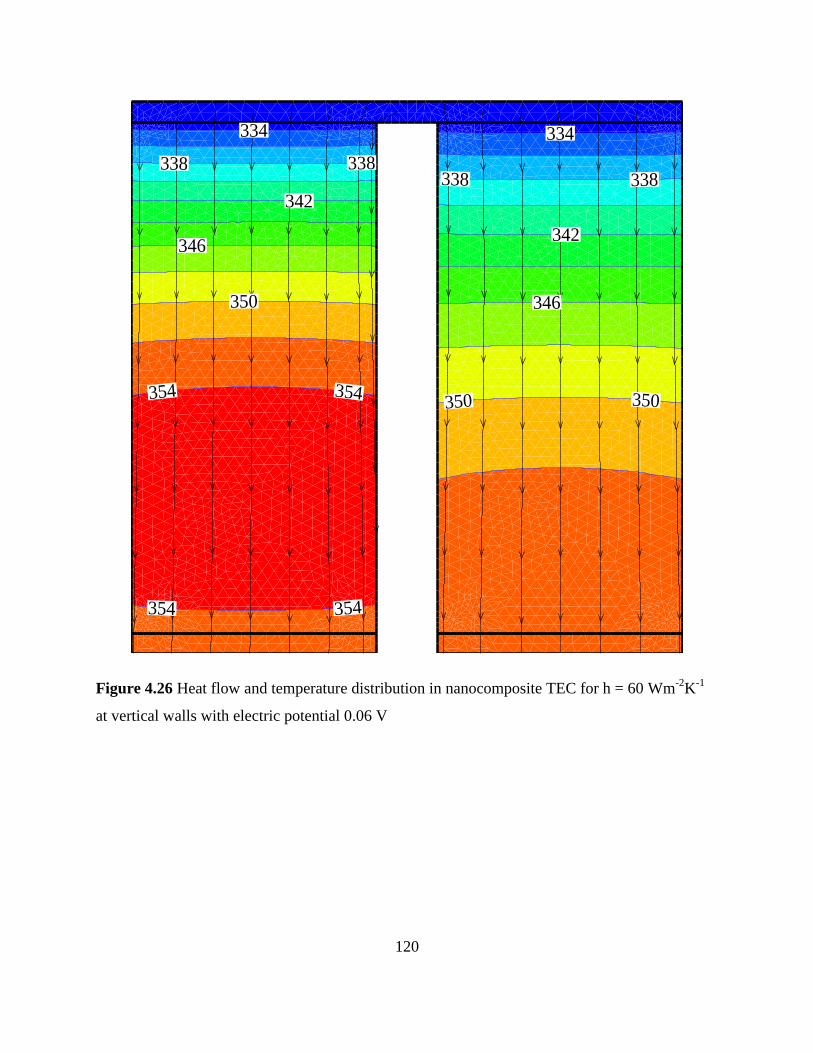
120

334

338 338

342

346

350

354 354

354354

334

338 338

342

346

350 350


K-1


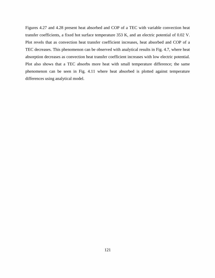
121

Figures 4.27 and 4.28 present heat absorbed and COP of a TEC with variable convection heat

transfer coefficients, a fixed hot surface temperature 353 K, and an electric potential of 0.02 V.

Plot revels that as convection heat transfer coefficient increases, heat absorbed and COP of a

TEC decreases. This phenomenon can be observed with analytical results in Fig. 4.7, where heat

absorption decreases as convection heat transfer coefficient increases with low electric potential.

Plot also shows that a TEC absorbs more heat with small temperature difference; the same

phenomenon can be seen in Fig. 4.11 where heat absorbed is plotted against temperature

differences using analytical model.

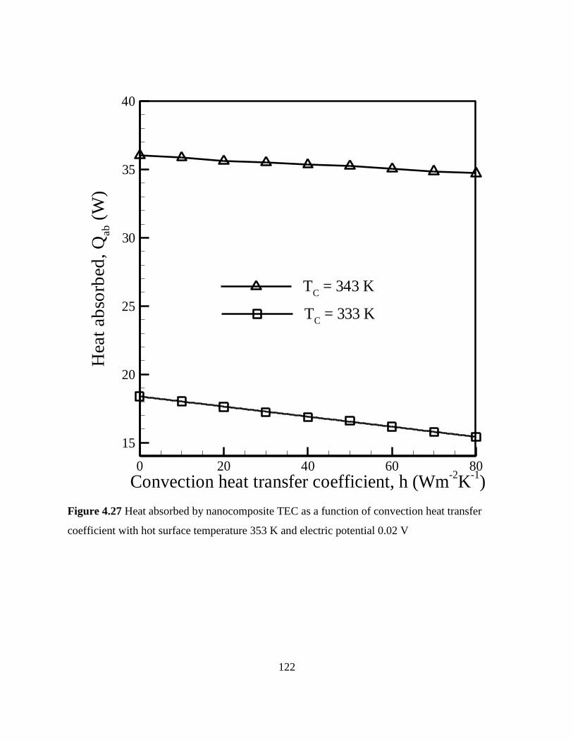
122

TC

= 343 K


K-1)

Hea

tab

sorb

ed,

Qab

(W)

0 20 40 60 80

15

20

25

30

35

40

TC

= 333 K

Figure 4.27 Heat absorbed by nanocomposite TEC as a function of convection heat transfer

coefficient with hot surface temperature 353 K and electric potential 0.02 V

123

TC

= 343 K


K-1)

CO

P

0 20 40 60 802

2.5

3

3.5

4

4.5

5

TC

= 333 K

Figure 4.28 COP of nanocomposite TEC as a function of convection heat transfer coefficient

with hot surface temperature 353 K and electric potential 0.02 V

124

In order to study the same phenomenon with large electric potential, heat absorbed and COP are

plotted as a function of convection heat transfer coefficient with a hot surface temperature 353 K

and an electric potential of 0.06 V in Figs. 4.29 and 4.30. Due to large electric potential TEC

produces more Joule heat and a leg of the TEC remains at higher temperature compared to

surroundings. This phenomenon is shown using contours and heat streamlines in Figs. 4.29 and

4.30. At higher convection heat transfer coefficients, a TE leg removes more heat to

surroundings which eventually assists more absorption of heat from the cold surface. It is

important to note here that COP of a TEC relatively remains same because of increment in power

input. Such large heat absorption can be helpful where amount of heat generation is large such as

large data centers.

125

TC

= 343 K


K-1)

Heat

ab

sorb

ed

,Q

ab

(W)

0 20 40 60 80100

105

110

115

120

125

TC

= 333 K

Figure 4.29 Heat absorbed by nanocomposite TEC as a function of convection heat transfer

coefficient with hot surface temperature 353 K and electric potential 0.06 V

126

TC

= 343 K


K-1)

CO

P

0 20 40 60 803.9

4

4.1

4.2

4.3

4.4

4.5

4.6

TC

= 333 K

Figure 4.30 COP of nanocomposite TEC as a function of convection heat transfer coefficient

with hot surface temperature 353 K and electric potential 0.06 V

127

Figures 4.31 and 4.32 present comparison between analytical and numerical simulation results.

Due to approximations such as decoupling between TE constitutive equations in analytical

modeling, analytical results over predict the heat absorbed and COP compared to numerical

simulations. Nevertheless, results show a fair agreement between analytical and numerical

simulations.

128

Numerical simulation results


K-1)

Hea

tab

sorb

ed,

Qab

(W)

0 20 40 60 8014

15

16

17

18

19

20

Analytical results

Figure 4.31 Comparison of analytical and numerical simulation results in terms of heat absorbed

considering variable convection heat transfer coefficient with hot surface temperature 353 K,

cold surface temperature 333 K, and electric potential 0.02 V

129



K-1)

CO

P

0 20 40 60 802.4

2.5

2.6

2.7

2.8

2.9

3

Analytical results

Figure 4.32 Comparison of analytical and numerical simulation results in terms of COP

considering variable convection heat transfer coefficient with hot surface temperature 353 K,

cold surface temperature 333 K, and electric potential 0.02 V

130

Figure 4.33 shows COP of a TEC using conventional (no nanostructuring) and nanocomposite

TE materials. The trend in a plot is quite evident about rise in the COP using nanocomposite TE

materials. COP of TEC increases from 4.92 to 5.58 if nanocomposite materials are used, which

gives approximately 13% rise for the materials considered. The rise in COP can be attributed to a

reduction in the thermal conductivity of TE materials due to nanostructuring. As observed from

Fig. 4.34, thermal conductivity of nanocomposite is lower than conventional TE materials. For

example, thermal conductivity of p-type BiSbTe decreases from 1.36 Wm-1

K-1

to 0.98 Wm-1

K-1

at 100 ºC.

131


CO

P

0 5 10 15 202.5

3

3.5

4

4.5

5

5.5

6

Conventional TE material

Nanocomposite TE material

Figure 4.33 Comparison of COP using conventional (no nanostructuring) and nanocomposite TE

material considering h ≈ 0 Wm-2

K-1

, hot surface temperature 353 K, and electric current input of

1 A

132

p-type conventional TE material

n-type conventional TE material

Temperature, T (C)

Th

erm

al

co

nd

ucti

vit

y,

k(W

m-1

K-1

)

0 50 100 150 200 2500.5

1

1.5

2

2.5

3

3.5

p-type nanocomposite TE material

n-type nanocomposite TE material

Figure 4.34 Thermal conductivity of conventional (no nanostructuring) and nanocomposite TE

materials

133

Figure 4.35 shows a comparison in terms of a temperature difference created by unit cell of a

TEC with different levels of electric current input. Poudel et al. (2008) prepared a p-type BiSbTe

nanostructured TE leg via hot pressing the ball-milled nanopowders of BiSbTe. They (Poudel et

al. 2008) prepared a unit cell of TEC using one p-type nanostructured TE leg and one n-type

commercially available (non-nanostructured) TE leg. Authors (Poudel et al. 2008) performed an

experiment under vacuum condition with a hot surface temperature 373 K to verify the

performance of a unit cell of a TEC. Results obtained from current work shows fair agreement

with an experimental work as presented in Fig. 4.35. The current results also show good

agreement with the theoretical predictions given in Poudel et al. (2008).

134

Electric current, I(A)

Tem

per

atu

red

iffe

ren

ce,

T(o

C)

0 2 4 6 8 100

20

40

60

80

100

120Poudel et al. (2008) experimental results

Current work

Poudel et al. (2008) Theoretical results

Figure 4.35 Comparison of results between current work and Poudel et al. (2008)

135

4.4 Conclusions

In this research work, a 1D analytical heat transfer model of a TEC was derived considering the

Seebeck effect, Peltier effect, Thomson effect, heat conduction, and convection heat transfer.

TEC performance parameters, such as the heat absorbed and COP, were analyzed as functions of

the electric current and convection heat transfer coefficient. In addition, an optimum electric

current is calculated considering different convection heat transfer coefficients and TE leg

heights for two different cases: maximum heat absorption, and maximum COP. A numerical

simulation was also performed to investigate heat transfer and temperature distribution in a

nanocomposite TEC.

The following conclusions are based on conducted studies:

1. Electric current plays a significant role in the performance of a TEC. As TE materials are

temperature-dependent and as the electric current can play a significant role in internal heat

generation, an optimum electric current input is an important factor.

2. It is observed that convection heat transfer has different effects on the performance of a TEC

depending on the amount of an electric current. At a low electric current input, it was

observed that convection heat transfer deteriorates the performance of a TEC, but at high

electric current, convection heat transfer can help remove large amount of heat from the cold

surface of a TEC.

3. This study demonstrates selection criteria to optimize TEC performance. For example, a

TEC can remove large amounts of heat but cannot exhibit higher COP, which can be useful

with high-end mainframes and large data centers where large heat generation is a major

problem.

In future, a more detailed study will be performed to experimentally study the effects of

convection heat transfer on the performance of a TEC.

136

4.5 Nomenclature


C1 a parameter (refer Eq.(9))

C2 a parameter (refer Eq.(9))

D thickness of TE leg (m)

E electric field intensity (Vm-1

)


K-1

)


J electric current density vector (Am-2

)


K-1

)

L height of TE leg (m)

p perimeter (m)

P electrical power output (W)


)

.q

heat generation rate (Wm-3

)

Q heat (W)

R electrical resistance (Ω)

T temperature (K)

W width of TE leg (m)

x co-ordinate system (m)


Greek Symbols


)

ε a parameter (refer Eq.(10))

κ a parameter (refer Eq.(10))

ρ electrical resistivity (Ωm)


)

τ Thomson coefficient (VK-1

)


ψ a parameter (refer Eq.(10))

137

Subscripts


ab heat absorbed

c convection heat loss

C cold surface temperature

eff effective transport properties

g gap between TE legs

gen heat generation

H hot surface temperature

i internal resistance

max maximum value

n n-type material

opt optimum value

p p-type material

re heat rejected

138

CHAPTER 5: EFFECT OF THERMAL CONDUCTIVITY ON

PERFORMANCE OF THERMOELECTRIC SYSTEMS BASED ON

EFFECTIVE MEDIUM THEORY

5.1 Introduction

Thermoelectric (TE) systems are typically made up of multiple pairs of p-type and n-type

semiconductor materials which are connected electrically in series and thermally in parallel. A

TE system working as a generator based on the Seebeck effect is called a thermoelectric

generator (TEG). Alternatively, a TE system working as a cooler/heater based on the Peltier

effect is called a thermoelectric cooler (TEC). TE systems have potential applications in

electronics, military, laboratory equipment, and transportation systems. TE systems offer many

advantages such as silent operation, compact design, robust operation, long service life, and

environmentally friendly. The performance of TE materials is measured using a parameter

called figure of merit (ZT = α2σT/k). Due to low ZT of TE materials, TE systems are redundant in

many real world applications. A poor electrical conductivity and Seebeck coefficient and higher

thermal conductivity leads to a poor ZT. Although, ZT can be improved in different ways and

two of the ways to improve ZT are illustrated in Fig. 5.1.

139

Figure 5.1 Different approaches to increase ZT of TE materials (Martin-Gonzalez 2013)

The first way employs an increase in the Seebeck coefficient and electrical conductivity,

collectively called the ‘power factor’, while the second way employs a decrease in the thermal

conductivity. Hicks and Dresselhaus (1993) discussed the concept of quantum wire (one

dimensional) for the TE materials. ZT increases because power factor (α2σ) improves due to one

dimensional structure but not significantly lowering the thermal conductivity (Hicks and

Dresselhaus 1993). A method to increase ZT was demonstrated experimentally by

Venkatasubramanian et al. (2001) where ZT of a p-type superlattice of Bi2Te3/Sb2Te3 (Bismuth-

Telluride-Antimony) improved from 1 to 2.4 due to the reduction in the thermal conductivity.

Improvements offered by Hicks and Dresselhaus (1993) and Venkatasubramanian et al. (2001)

were primarily for low dimensional structures such as quantum dots, wires, and superlattice

structures. Such structures can be employed limitedly in the real world applications due to the

complicated physical/chemical vapor deposition method and cost to manufacturing (Ma et al.

2013). There is another route to improve the ZT in bulk TE materials called ‘nanocomposite bulk

materials’ (Bottner and Konig 2013). Nanocomposite bulk materials, which can also be called as

‘composites’ are bulk materials with nanostructured features inside it (Ma et al. 2013).

Composites are made up of a base material and macro/nano particles which can be manufactured

140

via wet-chemical and mechanical synthesis techniques (e.g., solvothermal, extrusion, and high

energy milling). Scoville et al. (1995) reduced the thermal conductivity by 40% by adding Boron

Nitride and Boron Carbide particles into Silicon-Germanium composite. A bulk p-type BixSb2-

xTe3 composite prepared by hot-pressing nanopowders gave ZT of 1.4 due to the low thermal

conductivity (Poudel et al. 2008). In the similar manner, a Bi2Te3 with SiC (Silica Carbide)

nanoparticles (Zhao et al. 2008), Co4Sb12 (Skutterudites) (Li et al. 2009), and AgPbxSbTe2+x

(Lead Antimony Silver Telluride) (Hsu et al. 2004) reported improvement in ZT due to low

thermal conductivities of composites. Bulk composites with the low thermal conductivity

demonstrate promise of improved ZT and, more importantly, routes to synthesize them are more

cost-effective compared to low-dimensional structures (Ma et al. 2013). Thermal conductivities

of composites depend on various parameters, such as particle size, volume fraction, particle

shape, and thermal conductivities of base and particle materials. Thermal conductivities of

composites can be predicted by analytical models based on the Effective Medium Theory

(EMT). The EMT is a method of treating a macroscopically inhomogeneous medium in which

transport properties varies in space (Stroud 1998). EMTs have been applied to different

situations, such as Yu et al. (2015) applied the EMT to calculate the effective permittivity, Gong

et al. (2014) derived modified EMT for a porous media to model the thermal conductivity, Hou

et al. (2015) applied EMT to calculate the effective thermal conductivity of porous thin films,

and Chen et al. (2014) developed the effective thermal conductivity model for bentonites which

is considered engineered barrier material for radioactive wastes. The classical work of Rayleigh

(1892) and Maxwell (1954) can predict the transport properties of a mixture which can also be

applied to thermal conductivity of a composite as being one of the prime transport properties.

Maxwell (1954) considered a heterogeneous mixture with the spherical particles with thermal

conductivities of base material, particles, and composite as kb, kp, and keff, respectively. In

addition to this, is a volume fraction of particle inclusions. Equation (1) is an expression of the

effective thermal conductivity of a composite in terms of thermal conductivities of base and

particle materials and volume fraction of particles.

)(2

)(3

bpbp

bp

beffkkkk

kkkk

(1)

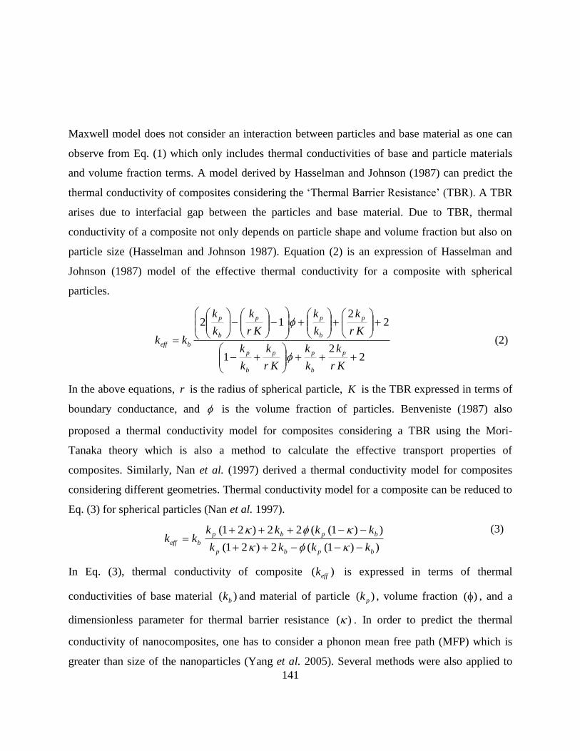
141

Maxwell model does not consider an interaction between particles and base material as one can

observe from Eq. (1) which only includes thermal conductivities of base and particle materials

and volume fraction terms. A model derived by Hasselman and Johnson (1987) can predict the

thermal conductivity of composites considering the ‘Thermal Barrier Resistance’ (TBR). A TBR

arises due to interfacial gap between the particles and base material. Due to TBR, thermal

conductivity of a composite not only depends on particle shape and volume fraction but also on

particle size (Hasselman and Johnson 1987). Equation (2) is an expression of Hasselman and

Johnson (1987) model of the effective thermal conductivity for a composite with spherical

particles.

22

1

22

12

Kr

k

k

k

Kr

k

k

k

Kr

k

k

k

Kr

k

k

k

kkp

b

pp

b

p

p

b

pp

b

p

beff

(2)

In the above equations, r is the radius of spherical particle, K is the TBR expressed in terms of

boundary conductance, and is the volume fraction of particles. Benveniste (1987) also

proposed a thermal conductivity model for composites considering a TBR using the Mori-

Tanaka theory which is also a method to calculate the effective transport properties of

composites. Similarly, Nan et al. (1997) derived a thermal conductivity model for composites

considering different geometries. Thermal conductivity model for a composite can be reduced to

Eq. (3) for spherical particles (Nan et al. 1997).

))1((2)21(

))1((22)21(

bpbp

bpbp

beffkkkk

kkkkkk

(3)

In Eq. (3), thermal conductivity of composite )( effk is expressed in terms of thermal

conductivities of base material )( bk and material of particle )( pk , volume fraction )( , and a

dimensionless parameter for thermal barrier resistance )( . In order to predict the thermal

conductivity of nanocomposites, one has to consider a phonon mean free path (MFP) which is

greater than size of the nanoparticles (Yang et al. 2005). Several methods were also applied to

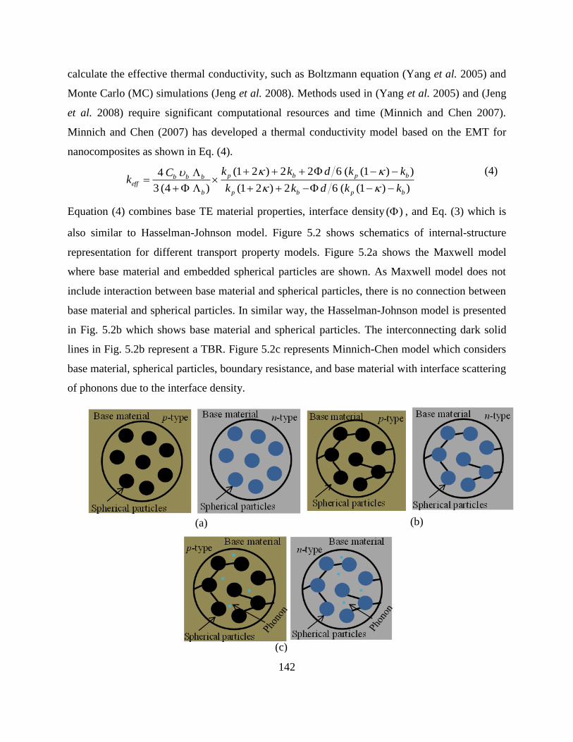
142

calculate the effective thermal conductivity, such as Boltzmann equation (Yang et al. 2005) and

Monte Carlo (MC) simulations (Jeng et al. 2008). Methods used in (Yang et al. 2005) and (Jeng

et al. 2008) require significant computational resources and time (Minnich and Chen 2007).

Minnich and Chen (2007) has developed a thermal conductivity model based on the EMT for

nanocomposites as shown in Eq. (4).

))1((62)21(

))1((622)21(

)4(3

4

bpbp

bpbp

b

bbbeff

kkdkk

kkdkkCk

(4)

Equation (4) combines base TE material properties, interface density )( , and Eq. (3) which is

also similar to Hasselman-Johnson model. Figure 5.2 shows schematics of internal-structure

representation for different transport property models. Figure 5.2a shows the Maxwell model

where base material and embedded spherical particles are shown. As Maxwell model does not

include interaction between base material and spherical particles, there is no connection between

base material and spherical particles. In similar way, the Hasselman-Johnson model is presented

in Fig. 5.2b which shows base material and spherical particles. The interconnecting dark solid

lines in Fig. 5.2b represent a TBR. Figure 5.2c represents Minnich-Chen model which considers

base material, spherical particles, boundary resistance, and base material with interface scattering

of phonons due to the interface density.

(c)

(a) (b)

143

Figure 5.2 Graphical representation of (a) Maxwell model (b) Hasselman and Johnson model (c)

Minnich and Chen model

Table 5.1 shows the comparison between the effective transport property models for macro and

nanocomposites in terms of the applicability and limitations.

Table 5.1 Comparison of different effective medium theories

Effective Medium Theories Applicability and Limitations

Maxwell model (Maxwell

1954)

Spherical particles embedded in spherical region, No

consideration thermal barrier resistance

Hasselman and

Johnson model (Hasselman

and Johnson 1987)

Spherical, cylindrical, and flat plate dispersions into host

material and thermal barrier resistance between particles and

base material, Valid for macro size particles

Minnich and Chen model

(Minnich and Chen 2007)

Spherical and cylindrical nanoparticle embedded in cube,

Valid for nano size particles

Yang and Stabler (2009) pointed out that high performance TE materials such as bulk

composites can expand the applications of TE systems. Thus, it is very important to study the

effects of a low thermal conductivity of TE bulk composites on the performance of TE systems.

To our best knowledge, authors are not aware of studies investigating the effect of low thermal

conductivities based on the EMT on the performance of TE systems. In this work, performance

of TE systems in a generator and cooler mode is investigated with three different effective

transport property models. Authors have considered Maxwell model, Hasselman-Johnson model,

and Minnich-Chen model. It is important to emphasize here that each model presents

modifications to their predecessor, for e.g., Maxwell model was first to consider the spherical

particles to calculate transport properties in a composite structure followed by Hasselman-

Johnson model, and last Minnich-Chen model. In addition to quantitative results, qualitative

results are also presented for a TEG and TEC system.

144

5.2 Modeling and boundary conditions

A schematic diagram of TE systems being investigated is shown in Fig. 5.3 with p-type and n-

type composite semiconductor legs. A copper strip connects semiconductor legs together. Each

semiconductor leg has a cross-sectional area of DW , height of H , and separated by a distance

dL . Qin and Qout are amounts of heat available at the heat source and heat sink, respectively.

During the subsequent analysis following assumptions are made:

Contact resistances at the interface of copper and TE legs are negligible.

TE system operates under a steady-state condition.

Figure 5.3 Schematic diagram of typical (a) TEC and (b) TEG system

The energy transport in TE system considering steady state can be expressed as (Antonova and

Looman 2005)

genpm qt

TC

q . (5)

where m , pC , T , q , and genq represent material density, specific heat, temperature, heat flux

vector, and volumetric heat generation, respectively. The continuity of electric charge through

the system must satisfy

Qin

(a)

n

W

p

T1

T2

I

Qout

H

Ld

x

T1 < T2 Qin

n

W

p

T1

T2

I

Qout

H

Ld

x

(b)

T1 > T2

qconv qconv

145

0

t

DJ . (6)


respectively. Equation (5) and Eq. (6) are coupled by the set of TE constitutive equations

(Antonova and Looman 2005) as shown in Eq. 7(a) and Eq. 7(b) below

TkT ][][ Jq

)][(][ T EJ

7(a)

7(b)

where ][ is the Seebeck coefficient matrix, ][k is the thermal conductivity matrix, ][ is the


expressed as , where is the electric scalar potential (Landau 1984).

Combining Eq. (5) to Eq. 7(b), the coupled TE equations for energy and charge transfers can be

expressed as

JEJ

TkT

t

TCpm ][][ (8)

0][][][][

Tt

(9)

where ][ is the dielectric permittivity matrix (Antonova and Looman 2005) and JE represents

Joule heat (Antonova and Looman 2005).

For a typical TE system shown in Fig. 5.3 thermal boundary conditions are as follow:

At the top surface ( 0x ) temperature is constant ( 1TT )

At the bottom surface ( Hx ) temperature is constant ( 2TT )

Convection heat transfer from the side surfaces to the surrounding, )(conv aTThq

where Ta is atmospheric temperature and h is convection heat transfer coefficient.

Note that the material property matrices (e.g., ][ and ][k , etc.) are suitable for non-

homogeneous materials. These material property matrices become a single-valued property in the

case of homogeneous materials. Initially, a simplified 1-D version of above equations will be

solved to obtain the close forms of analytical solutions.

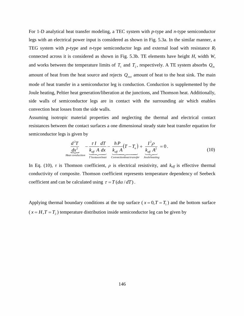
146

For 1-D analytical heat transfer modeling, a TEC system with p-type and n-type semiconductor

legs with an electrical power input is considered as shown in Fig. 5.3a. In the similar manner, a

TEG system with p-type and n-type semiconductor legs and external load with resistance Rl

connected across it is considered as shown in Fig. 5.3b. TE elements have height H, width W,

and works between the temperature limits of 1T and 2T , respectively. A TE system absorbs inQ

amount of heat from the heat source and rejects outQ amount of heat to the heat sink. The main

mode of heat transfer in a semiconductor leg is conduction. Conduction is supplemented by the

Joule heating, Peltier heat generation/liberation at the junctions, and Thomson heat. Additionally,

side walls of semiconductor legs are in contact with the surrounding air which enables

convection heat losses from the side walls.

Assuming isotropic material properties and neglecting the thermal and electrical contact

resistances between the contact surfaces a one dimensional steady state heat transfer equation for

semiconductor legs is given by

0

2

2

hom

2

2

heatingJoule

eff

transferheatConvection

a

eff

heatsonT

eff

conductionHeat

Ak

ITT

Ak

Ph

dx

dT

Ak

I

dx

Td .

(10)

In Eq. (10), τ is Thomson coefficient, ρ is electrical resistivity, and keff is effective thermal

conductivity of composite. Thomson coefficient represents temperature dependency of Seebeck

coefficient and can be calculated using )/( dTdT .

Applying thermal boundary conditions at the top surface ( 1,0 TTx ) and the bottom surface

( 2, TTHx ) temperature distribution inside semiconductor leg can be given by

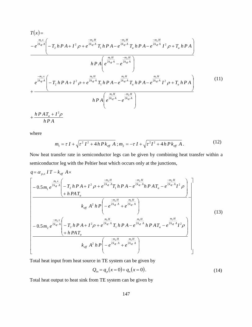
147

APh

ITAPh

eeAPh

APhTIeAPhTeAPhTeIAPhTe

eeAPh

APhTIeAPhTeAPhTeIAPhTe

xT

a

Ak

Hm

Ak

Hm

a

Ak

Hm

a

Ak

Hm

Ak

Hm

Ak

xm

Ak

Hm

Ak

Hm

a

Ak

Hm

a

Ak

Hm

Ak

Hm

Ak

xm

effeff

effeffeffeff

effeff

effeffeffeff

2

22

222

1

22

2

2

22

222

1

22

2

2

21

1112

21

2221

(11)

where

AkPhIIm eff422

1 ; AkPhIIm eff422

2 . (12)

Now heat transfer rate in semiconductor legs can be given by combining heat transfer within a

semiconductor leg with the Peltier heat which occurs only at the junctions,

Ak

Hm

Ak

Hm

eff

a

Ak

Hm

a

Ak

Hm

Ak

Hm

Ak

xm

Ak

Hm

Ak

Hm

eff

a

Ak

Hm

a

Ak

Hm

Ak

Hm

Ak

xm

effnp

effeff

effeffeffeff

effeff

effeffeffeff

eePhAk

TPAh

IeTAPheAPhTeIAPhTem

eePhAk

TPAh

IeTAPheAPhTeIAPhTem

AkTIq

222

222

1

22

22

2

222

222

1

22

22

1

,

12

1112

12

2221

5.0

5.0

(13)

Total heat input from heat source in TE system can be given by

00 xqxqQ npin . (14)

Total heat output to heat sink from TE system can be given by

148

HxqHxqQ npout . (15)

COP of TEC (Fig. 5.3a) can be calculated from the following equation:

i

in

RI

QCOP

2 , (16)

while the thermal efficiency of TEG (Fig. 5.3b) can be calculated from the following equation:

in

outin

Q

QQ . (17)

It is important to note here that when convection heat transfer from the side walls of

semiconductor legs are extremely low ( 0h ) and if temperature dependency of TE materials is

negligible then heat input to TE system (Eq. (14)) reduces to

H

T

Ak

HI

H

TAkTIQ

eff

effnpin1

2

2

21,

2

. (18)

In similar manner, heat output to heat sink (Eq. (15)) becomes

H

T

H

T

Ak

HIAkTIQ

eff

effnpout12

2

2

2,2

. (19)


In this section, analytical and numerical simulation results are presented which are obtained

considering three different models of the effective transport properties based on the EMT.

Maxwell model, Hasselaman - Johnson model, and Minnich-Chen model are applied to calculate

effective thermal conductivities. Results are presented in terms of the effective thermal

conductivity of TE materials, COP, and thermal efficiency of TE systems. For a p-type TE

material, Bi2Te3 as a base material and Sb2Te3 particles are selected. The size of the Sb2Te3

particles varies from micrometer to nanometer. For n-type TE material, Bi2Te3 is considered

which can be used as a base material and nanoparticles. Table 5.2 (Pattamatta and Madnia 2009)

presents some properties (bulk thermal conductivity, volumetric specific heat, bulk MFP, and

phonon group velocity) of Bi2Te3 and Sb2Te3 which can be used to calculate the effective thermal

conductivity based on the Minnich-Chen model. Note that the bulk MFP can be defined as the

averaged distance travelled by an energy carrier per collision over a sufficient number of

collisions (Tzou 2014), while the phonon group velocity represents velocity of phonons, a quasi-

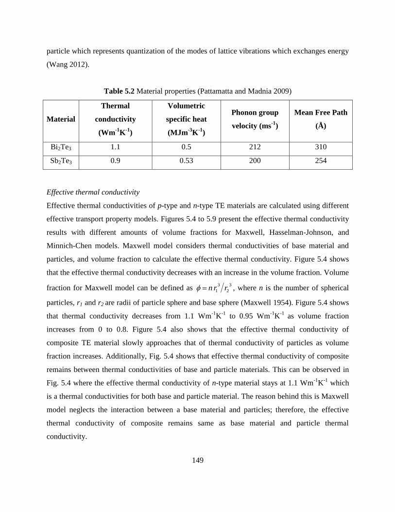
149

particle which represents quantization of the modes of lattice vibrations which exchanges energy

(Wang 2012).

Table 5.2 Material properties (Pattamatta and Madnia 2009)

Material

Thermal

conductivity

(Wm-1

K-1

)

Volumetric

specific heat

(MJm-3

K-1

)

Phonon group

velocity (ms-1

)

Mean Free Path

(Å)

Bi2Te3 1.1 0.5 212 310

Sb2Te3 0.9 0.53 200 254

Effective thermal conductivity

Effective thermal conductivities of p-type and n-type TE materials are calculated using different

effective transport property models. Figures 5.4 to 5.9 present the effective thermal conductivity

results with different amounts of volume fractions for Maxwell, Hasselman-Johnson, and

Minnich-Chen models. Maxwell model considers thermal conductivities of base material and

particles, and volume fraction to calculate the effective thermal conductivity. Figure 5.4 shows

that the effective thermal conductivity decreases with an increase in the volume fraction. Volume

fraction for Maxwell model can be defined as 3

2

3

1 rrn , where n is the number of spherical

particles, r1 and r2 are radii of particle sphere and base sphere (Maxwell 1954). Figure 5.4 shows

that thermal conductivity decreases from 1.1 Wm-1

K-1

to 0.95 Wm-1

K-1

as volume fraction

increases from 0 to 0.8. Figure 5.4 also shows that the effective thermal conductivity of

composite TE material slowly approaches that of thermal conductivity of particles as volume

fraction increases. Additionally, Fig. 5.4 shows that effective thermal conductivity of composite

remains between thermal conductivities of base and particle materials. This can be observed in

Fig. 5.4 where the effective thermal conductivity of n-type material stays at 1.1 Wm-1

K-1

which

is a thermal conductivities for both base and particle material. The reason behind this is Maxwell

model neglects the interaction between a base material and particles; therefore, the effective

thermal conductivity of composite remains same as base material and particle thermal

conductivity.

150

kef

f(W

m-1

K-1

)

0 0.2 0.4 0.6 0.80.9

0.95

1

1.05

1.1

1.15

n-type material

p-type material

Figure 5.4 Effective thermal conductivity of p-type and n-type thermoelectric material based on

Maxwell model

151

Figure 5.5 shows results of the effective thermal conductivity using Hasselman-Johnson model.

Figure 5.5 shows significant reduction in the effective thermal conductivity as volume fraction

increases. The effective thermal conductivity predicted by Hasselman-Johnson model is much

lower than Maxwell model for similar amount of volume fraction. For example, the effective

thermal conductivity using Hasselman – Johnson model with volume fraction 0.5 is 0.44

Wm-1

K-1

, whereas with similar volume fraction Maxwell model predicts effective thermal

conductivity of 0.99 Wm-1

K-1

. The drop in the magnitude of effective thermal conductivity is due

to the TBR which is represented by boundary conductance (K). The effective thermal

conductivity of TE material drops to 0.15 Wm-1

K-1

with volume fraction 0.8 and extremely low

(10-15

) boundary conductance considering Hasselman-Johnson model. If boundary conductance

remains very high (→∞) then effective thermal conductivity based on Hasselman – Johnson

model approaches to that of Maxwell model. This can be verified using Figs. 5.6 and 5.7 where

the effective thermal conductivity is plotted against boundary conductance at higher boundary

conductance. It is important to note here that in order to show effects of TBR, very low boundary

conductance (=10-15

) and very high boundary conductance (→∞) are taken arbitrarily.

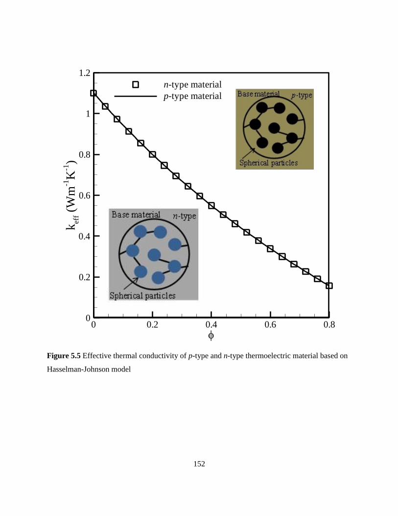
152

kef

f(W

m-1

K-1

)

0 0.2 0.4 0.6 0.80

0.2

0.4

0.6

0.8

1

1.2

n-type material

p-type material

Figure 5.5 Effective thermal conductivity of p-type and n-type thermoelectric material based on


153

As shown in Figs. 5.6 and 5.7, the effective thermal conductivity remains same as the thermal

conductivity of the base material when volume fraction is zero. With an increase in the volume

fraction, the effective thermal conductivity decreases. Moreover, an increase in the boundary

conductance leads to an increase in the effective thermal conductivity. Figures 5.6 and 5.7 also

show that the trend for p-type and n-type remains different as thermal conductivity of particles is

different for both materials.

154

K (Wm-2

K-1)

keff

(Wm

-1K

-1)

0 20000 40000 60000 80000 1000000

0.2

0.4

0.6

0.8

1

1.2

=0

=0.2

=0.4

=0.6

=0.8

Figure 5.6 Effect of thermal boundary conductance on effective thermal conductivity of p-type

using Hasselman-Johnson model

155

K (Wm-2

K-1)

keff

(Wm

-1K

-1)

0 20000 40000 60000 80000 1000000

0.2

0.4

0.6

0.8

1

1.2

=0

=0.2

=0.4

=0.6

=0.8

Figure 5.7 Effect of thermal boundary conductance on effective thermal conductivity of n-type

using Hasselman-Johnson model

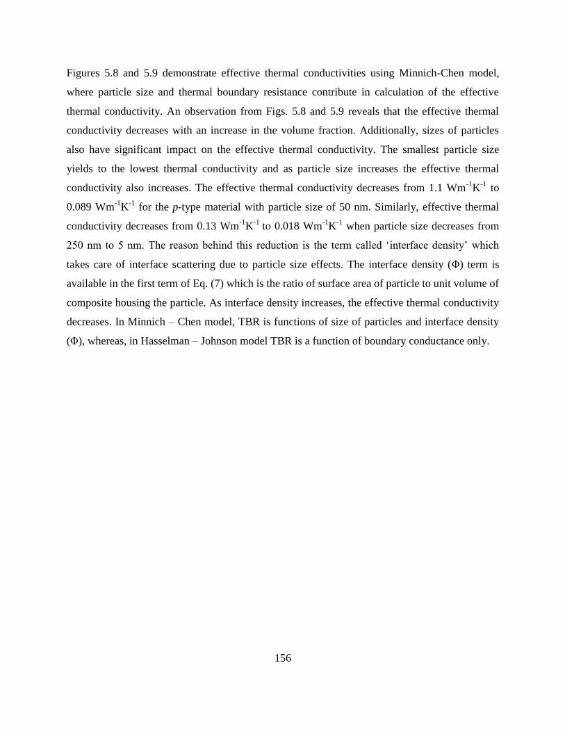
156

Figures 5.8 and 5.9 demonstrate effective thermal conductivities using Minnich-Chen model,

where particle size and thermal boundary resistance contribute in calculation of the effective

thermal conductivity. An observation from Figs. 5.8 and 5.9 reveals that the effective thermal

conductivity decreases with an increase in the volume fraction. Additionally, sizes of particles

also have significant impact on the effective thermal conductivity. The smallest particle size

yields to the lowest thermal conductivity and as particle size increases the effective thermal

conductivity also increases. The effective thermal conductivity decreases from 1.1 Wm-1

K-1

to

0.089 Wm-1

K-1

for the p-type material with particle size of 50 nm. Similarly, effective thermal

conductivity decreases from 0.13 Wm-1

K-1

to 0.018 Wm-1

K-1

when particle size decreases from

250 nm to 5 nm. The reason behind this reduction is the term called ‘interface density’ which

takes care of interface scattering due to particle size effects. The interface density (Φ) term is

available in the first term of Eq. (7) which is the ratio of surface area of particle to unit volume of

composite housing the particle. As interface density increases, the effective thermal conductivity

decreases. In Minnich – Chen model, TBR is functions of size of particles and interface density

(Φ), whereas, in Hasselman – Johnson model TBR is a function of boundary conductance only.

157

kef

f(W

m-1

K-1

)

0 0.2 0.4 0.6 0.80

0.2

0.4

0.6

0.8

1

1.2d = 5 nm

d = 15 nm

d = 50 nm

d = 100 nm

d = 250 nm

Figure 5.8 Effective thermal conductivity of p-type thermoelectric material using Minnich-Chen

model

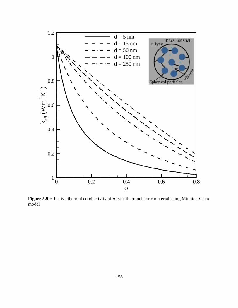
158

kef

f(W

m-1

K-1

)

0 0.2 0.4 0.6 0.80

0.2

0.4

0.6

0.8

1

1.2d = 5 nm

d = 15 nm

d = 50 nm

d = 100 nm

d = 250 nm

Figure 5.9 Effective thermal conductivity of n-type thermoelectric material using Minnich-Chen

model

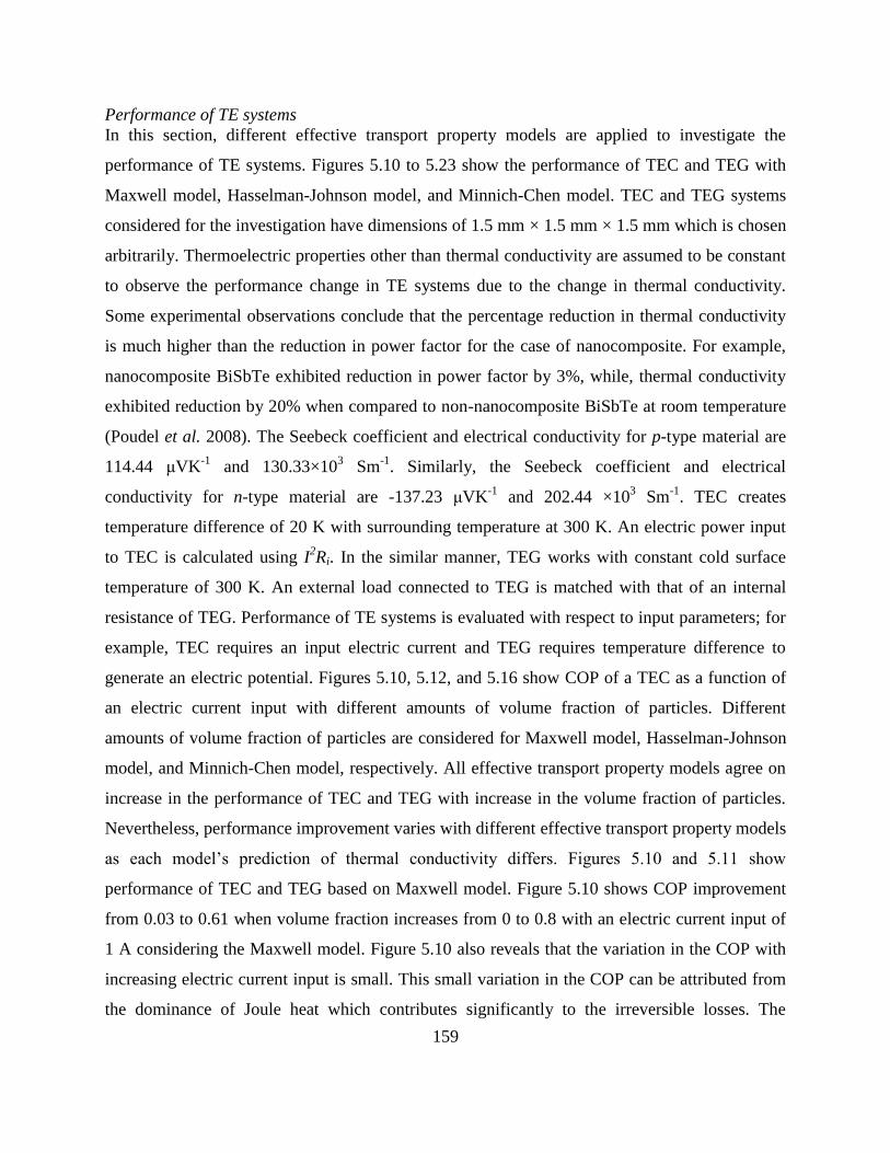
159

Performance of TE systems

In this section, different effective transport property models are applied to investigate the

performance of TE systems. Figures 5.10 to 5.23 show the performance of TEC and TEG with

Maxwell model, Hasselman-Johnson model, and Minnich-Chen model. TEC and TEG systems

considered for the investigation have dimensions of 1.5 mm × 1.5 mm × 1.5 mm which is chosen

arbitrarily. Thermoelectric properties other than thermal conductivity are assumed to be constant

to observe the performance change in TE systems due to the change in thermal conductivity.

Some experimental observations conclude that the percentage reduction in thermal conductivity

is much higher than the reduction in power factor for the case of nanocomposite. For example,

nanocomposite BiSbTe exhibited reduction in power factor by 3%, while, thermal conductivity

exhibited reduction by 20% when compared to non-nanocomposite BiSbTe at room temperature

(Poudel et al. 2008). The Seebeck coefficient and electrical conductivity for p-type material are

114.44 μVK-1

and 130.33×103 Sm

-1. Similarly, the Seebeck coefficient and electrical

conductivity for n-type material are -137.23 μVK-1

and 202.44 ×103 Sm

-1. TEC creates

temperature difference of 20 K with surrounding temperature at 300 K. An electric power input

to TEC is calculated using I2Ri. In the similar manner, TEG works with constant cold surface

temperature of 300 K. An external load connected to TEG is matched with that of an internal

resistance of TEG. Performance of TE systems is evaluated with respect to input parameters; for

example, TEC requires an input electric current and TEG requires temperature difference to

generate an electric potential. Figures 5.10, 5.12, and 5.16 show COP of a TEC as a function of

an electric current input with different amounts of volume fraction of particles. Different

amounts of volume fraction of particles are considered for Maxwell model, Hasselman-Johnson

model, and Minnich-Chen model, respectively. All effective transport property models agree on

increase in the performance of TEC and TEG with increase in the volume fraction of particles.

Nevertheless, performance improvement varies with different effective transport property models

as each model’s prediction of thermal conductivity differs. Figures 5.10 and 5.11 show

performance of TEC and TEG based on Maxwell model. Figure 5.10 shows COP improvement

from 0.03 to 0.61 when volume fraction increases from 0 to 0.8 with an electric current input of

1 A considering the Maxwell model. Figure 5.10 also reveals that the variation in the COP with

increasing electric current input is small. This small variation in the COP can be attributed from

the dominance of Joule heat which contributes significantly to the irreversible losses. The

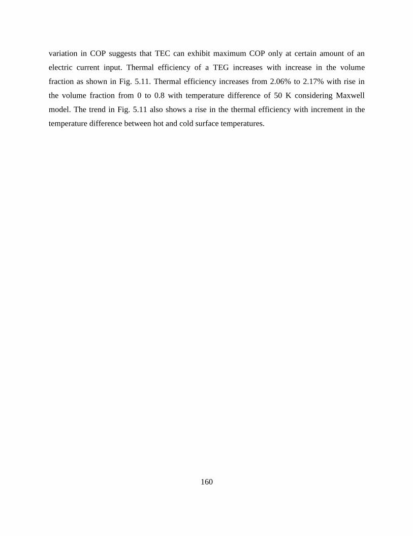
160

variation in COP suggests that TEC can exhibit maximum COP only at certain amount of an

electric current input. Thermal efficiency of a TEG increases with increase in the volume

fraction as shown in Fig. 5.11. Thermal efficiency increases from 2.06% to 2.17% with rise in

the volume fraction from 0 to 0.8 with temperature difference of 50 K considering Maxwell

model. The trend in Fig. 5.11 also shows a rise in the thermal efficiency with increment in the

temperature difference between hot and cold surface temperatures.

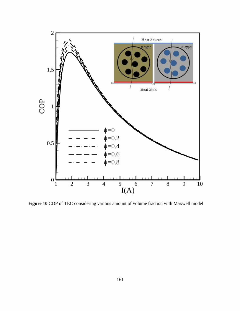
161

I(A)

CO

P

1 2 3 4 5 6 7 8 9 100

0.5

1

1.5

2

=0

=0.2

=0.4

=0.6

=0.8

Figure 10 COP of TEC considering various amount of volume fraction with Maxwell model

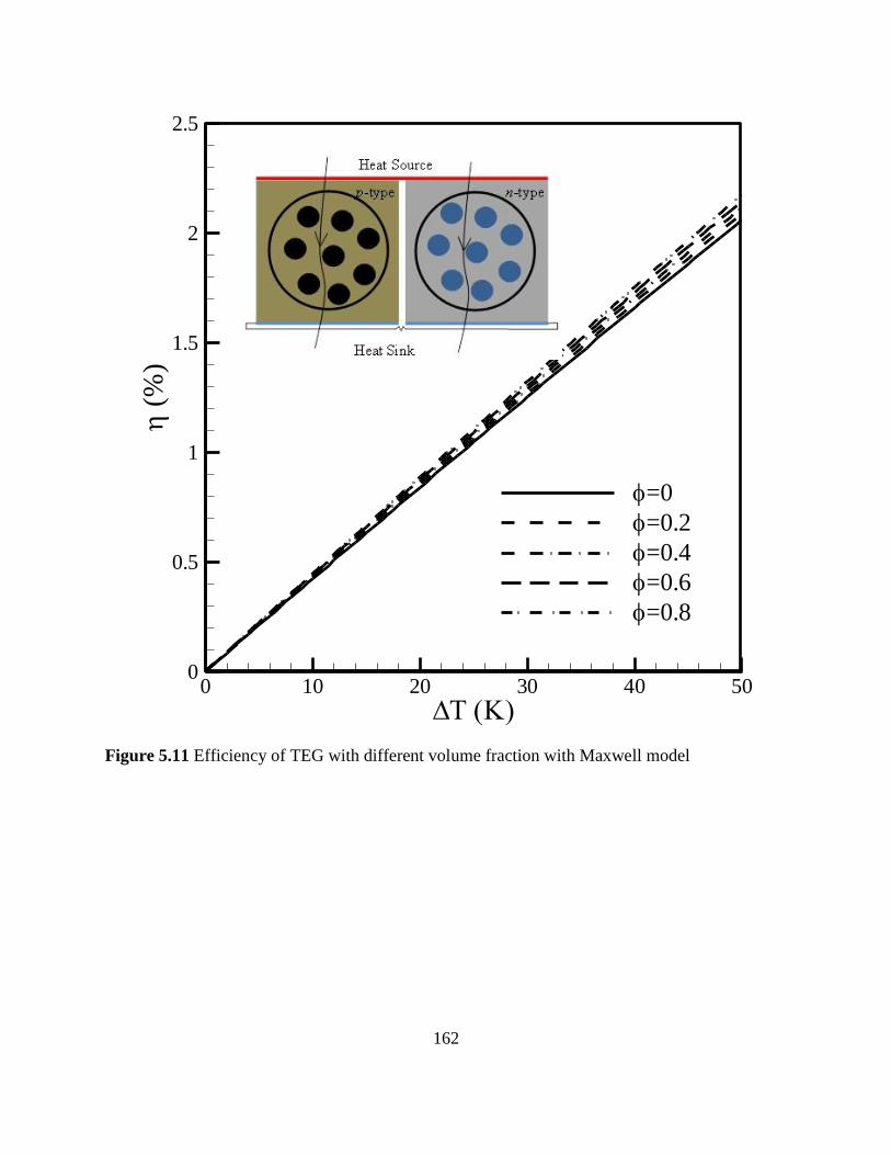
162

(%

)

0 10 20 30 40 500

0.5

1

1.5

2

2.5

=0

=0.2

=0.4

=0.6

=0.8

Figure 5.11 Efficiency of TEG with different volume fraction with Maxwell model

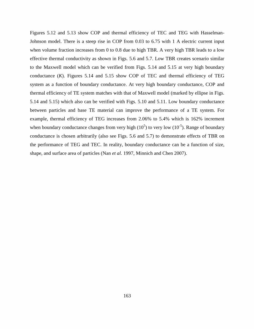
163

Figures 5.12 and 5.13 show COP and thermal efficiency of TEC and TEG with Hasselman-

Johnson model. There is a steep rise in COP from 0.03 to 6.75 with 1 A electric current input

when volume fraction increases from 0 to 0.8 due to high TBR. A very high TBR leads to a low

effective thermal conductivity as shown in Figs. 5.6 and 5.7. Low TBR creates scenario similar

to the Maxwell model which can be verified from Figs. 5.14 and 5.15 at very high boundary

conductance (K). Figures 5.14 and 5.15 show COP of TEC and thermal efficiency of TEG

system as a function of boundary conductance. At very high boundary conductance, COP and

thermal efficiency of TE system matches with that of Maxwell model (marked by ellipse in Figs.

5.14 and 5.15) which also can be verified with Figs. 5.10 and 5.11. Low boundary conductance

between particles and base TE material can improve the performance of a TE system. For

example, thermal efficiency of TEG increases from 2.06% to 5.4% which is 162% increment

when boundary conductance changes from very high (105) to very low (10

-5). Range of boundary

conductance is chosen arbitrarily (also see Figs. 5.6 and 5.7) to demonstrate effects of TBR on

the performance of TEG and TEC. In reality, boundary conductance can be a function of size,

shape, and surface area of particles (Nan et al. 1997, Minnich and Chen 2007).

164

I(A)

CO

P

1 2 3 4 5 6 7 8 9 100

1

2

3

4

5

6

7

=0

=0.2

=0.4

=0.6

=0.8

Figure 5.12 COP of TEC considering different amount of volume fraction with Hasselman

model

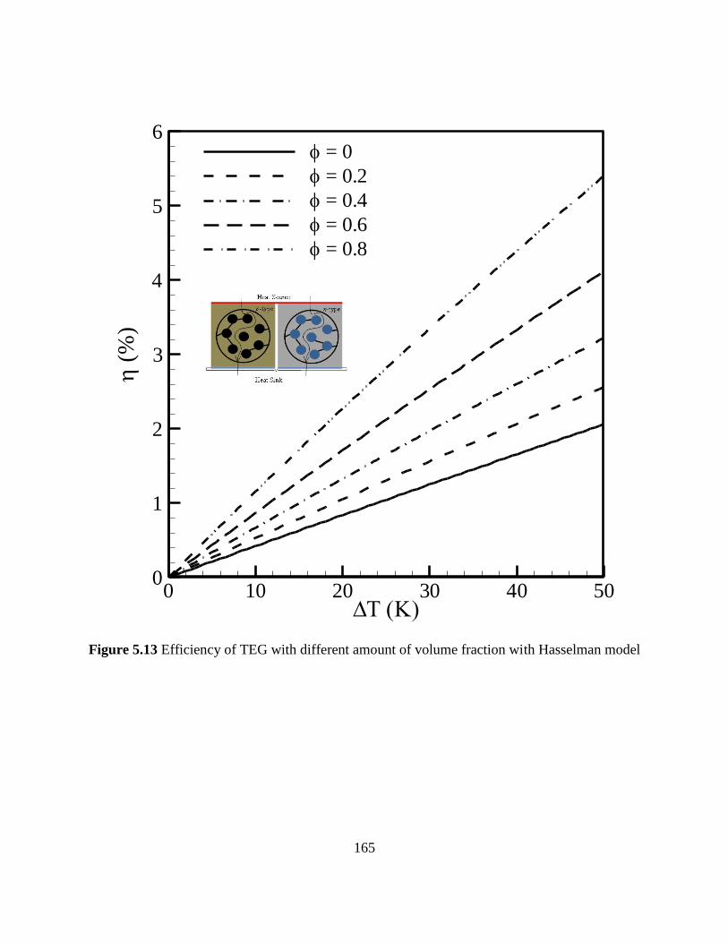
165

(%

)

0 10 20 30 40 500

1

2

3

4

5

6 = 0

= 0.2

= 0.4

= 0.6

= 0.8

Figure 5.13 Efficiency of TEG with different amount of volume fraction with Hasselman model

166

K (Wm-2

K-1)

CO

P

0 20000 40000 60000 80000 100000

0

1

2

3

4

5

6

7

=0

=0.2

=0.4

=0.6

=0.8

Figure 5.14 Effect of boundary conductance on performance of TEC based on Hasselman-

Johnson model

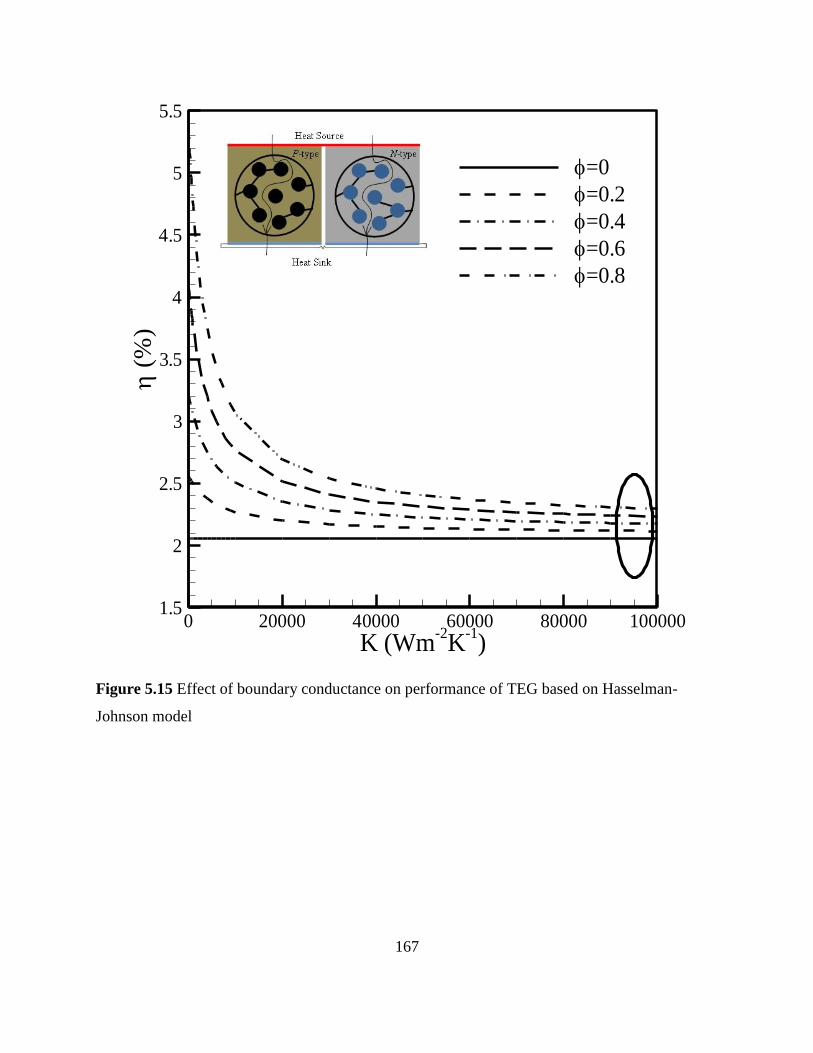
167

K (Wm-2

K-1)

(%

)

0 20000 40000 60000 80000 1000001.5

2

2.5

3

3.5

4

4.5

5

5.5

=0

=0.2

=0.4

=0.6

=0.8

Figure 5.15 Effect of boundary conductance on performance of TEG based on Hasselman-

Johnson model

168

Figures 5.16 and 5.17 show performance of a TE system based on Minnich-Chen model with

radius of spherical particle as 5 nm, which is chosen arbitrarily. Similar to other models

Minnich-Chen model also predicts increase in the performance of TE system with increase in

volume fraction as shown in Figs. 5.16 and 5.17. For example, thermal efficiency of TEG

increases from 2.06 % to 7.03 % (Fig. 5.17). Additionally, size of particles can affect the

effective thermal conductivity (Figs. 5.8 and 5.9) which eventually influences the performance of

TEG and TEC. Figures 5.18 and 5.19 show the effect of particle size on the performance of a

TEG and TEC. COP decreases as size of nanoparticle increases which is consistent with rise in

the effective thermal conductivity as shown in Figs. 5.8 and 5.9.

169

I (A)

CO

P

1 2 3 4 5 6 7 8 9 100

2

4

6

8

=0

=0.2

=0.4

=0.6

=0.8

Figure 5.16 COP of TEC considering different amount of volume fraction with Minnich-Chen

model

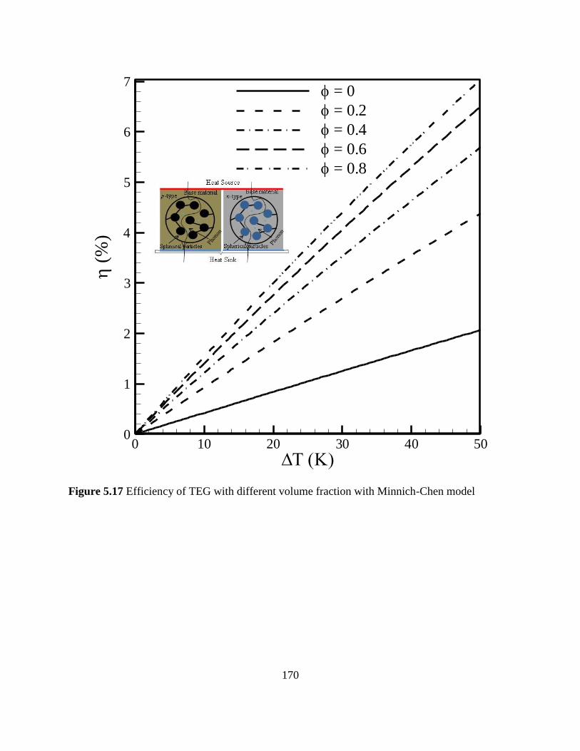
170

(%

)

0 10 20 30 40 500

1

2

3

4

5

6

7 = 0

= 0.2

= 0.4

= 0.6

= 0.8

Figure 5.17 Efficiency of TEG with different volume fraction with Minnich-Chen model

171

d (m)

CO

P

0 2E-08 4E-08 6E-08 8E-08 1E-07-1

0

1

2

3

4

5

6

7

8

9

10

11

=0

=0.2

=0.4

=0.6

=0.8

Figure 5.18 Effect of nanoparticle size on performance of TEC considering Minnich-Chen

model

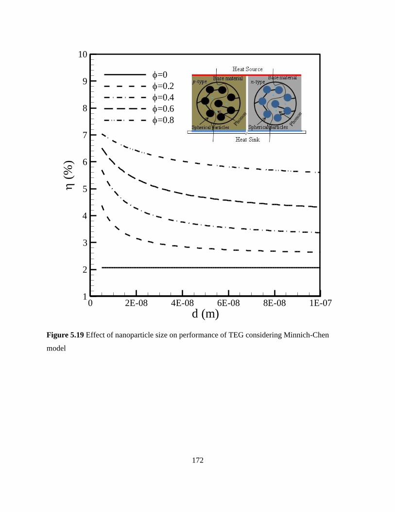
172

d (m)

(%

)

0 2E-08 4E-08 6E-08 8E-08 1E-071

2

3

4

5

6

7

8

9

10

=0

=0.2

=0.4

=0.6

=0.8

Figure 5.19 Effect of nanoparticle size on performance of TEG considering Minnich-Chen

model

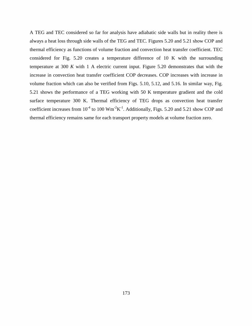
173

A TEG and TEC considered so far for analysis have adiabatic side walls but in reality there is

always a heat loss through side walls of the TEG and TEC. Figures 5.20 and 5.21 show COP and

thermal efficiency as functions of volume fraction and convection heat transfer coefficient. TEC

considered for Fig. 5.20 creates a temperature difference of 10 K with the surrounding

temperature at 300 K with 1 A electric current input. Figure 5.20 demonstrates that with the

increase in convection heat transfer coefficient COP decreases. COP increases with increase in

volume fraction which can also be verified from Figs. 5.10, 5.12, and 5.16. In similar way, Fig.

5.21 shows the performance of a TEG working with 50 K temperature gradient and the cold

surface temperature 300 K. Thermal efficiency of TEG drops as convection heat transfer

coefficient increases from 10-4

to 100 Wm-2

K-1

. Additionally, Figs. 5.20 and 5.21 show COP and

thermal efficiency remains same for each transport property models at volume fraction zero.

174

h = 10-4

Wm-2K

-1

h = 100 Wm-2K

-1

Minnich-Chen model

CO

P

0 0.2 0.4 0.6 0.82

3

4

5

6

7

8

9

10

h = 10-4

Wm-2K

-1

h = 100 Wm-2K

-1

Maxwell model

h = 10-4

Wm-2K

-1

h = 100 Wm-2

K-1


Figure 5.20 Performance of TEC with variable volume fractions and convection heat transfer

coefficients through side walls of TE legs

175

h = 10-4

Wm-2

K-1

h = 100 Wm-2K

-1

Minnich-Chen model

(%

)

0 0.2 0.4 0.6 0.81

2

3

4

5

6

h = 10-4

Wm-2K

-1

h = 100 Wm-2K

-1Maxwell model

h = 10-4

Wm-2

K-1

h = 100 Wm-2

K-1

Hasselman - Johnson model

Figure 5.21 Performance of TEG with variable volume fractions and convection heat transfer

coefficients through side walls of TE legs

176

The results reported so far indicate improved performances of a TEC and TEG using different

effective transport property models; however, predicted results are different for different

transport property models. For example, Maxwell model, Hasselman-Johnson model, and

Minnich-Chen model show COP of 0.61, 6.76, and 7.69, respectively, with an electric current

input of 1 A and volume fraction of 0.8. The reason behind such difference is the reduction in the

effective thermal conductivity in each transport property model with highest thermal

conductivity in Maxwell model and lowest in Minnich-Chen model. Higher or lower thermal

conductivity significantly effects the heat conduction part of total heat transfer in a TE system.

Figures 5.22 and 5.23 explain how effective thermal conductivity influences the heat conduction

portion of total heat input to TE system. Figure 5.22 shows heat conduction portion to total heat

input (Qin) in TEC as a function of volume fraction. TEC creates temperature difference of 20 K

with surrounding temperature 300 K and an electric current input of 1 A. As one can be observed

from Fig. 5.22 that increase in the volume fraction decreases the amount of heat conduction

which eventually contributes to rise in COP. A rise in COP can be verified from Figs. 5.10, 5.12,

and 5.16 which is due to the drop in effective thermal conductivity as already presented in Figs.

5.4, 5.5 and 5.8. In the similar way, heat conduction through TEG with temperature gradient of

50 K with cold surface temperature 300 K is plotted in Fig. 5.23. Heat conduction in TEG also

follows similar trend as that of TEC showing decreasing trend as volume fraction increases due

to the drop in the effective thermal conductivity. For a TEC system, heat removed can be higher

if heat conduction and Joule heating remain as low as possible. For a TEG system, it is very

important to maintain high temperature gradient to generate higher electric potential. Heat

conduction and Joule heating should remain as low as possible to maintain higher temperature

gradient and thus higher electric potential. It is important to note here that Peltier heat and Joule

heat remains unchanged because change in the effective thermal conductivity only influences

heat conduction through TE system.

177

Qin

(Co

nd

ucti

on

)(W

)

0 0.2 0.4 0.6 0.80

0.01

0.02

0.03

0.04

0.05

0.06

0.07


Maxwell model

Minnich-Chen model

Figure 5.22 Influence of effective thermal conductivity on heat conduction in TEC

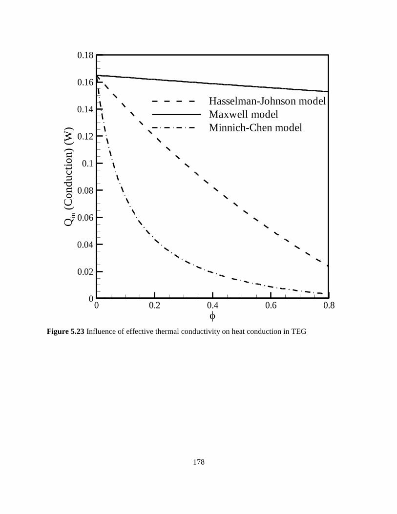
178

Qin

(Co

nd

ucti

on

)(W

)

0 0.2 0.4 0.6 0.80

0.02

0.04

0.06

0.08

0.1

0.12

0.14

0.16

0.18


Maxwell model

Minnich-Chen model

Figure 5.23 Influence of effective thermal conductivity on heat conduction in TEG

179


In this section, results achieved by solving Eq. (8) and (9) using the Finite Element Method are

presented based on discretization and solution techniques available in Mahmud and Pop (2006).

Initially, results obtained from numerical solutions are expressed using the field plots of

temperature contours, heat flow lines, electric potential contours, and electric current flow lines.

A composite TE system with width (W = 1.5 mm) and height (H = 1.5 mm) is considered for the

analysis. Both legs are separated by distance Ld = 0.2 mm. Maxwell model, Hasselman-Johnson

model, and Minnich-Chen model are applied to calculate the effective thermal conductivity. The

performance variation in TEG and TEC due to change in effective thermal conductivity is

observed. The Seebeck coefficient and electrical conductivity are assumed to be constant for

each simulation. Figures 5.24 to 5.28 represent field plots of temperature and electric potential

for a composite TEC. An electric potential is indicated by marked iso-potential lines with a

multi-colored background, while electric current flow is indicated by lines with arrows in Fig.

5.24. Similarly, temperature is presented by marked isothermal lines with multi-colored

background, while heat flow is presented by lines with arrows in Fig. 5.25 to 5.28. Composite

TEC maintains temperature difference of 10 K with surrounding temperature at 300 K and

electric potential of 0.02 V. Similarly, a TEG works between temperature gradient of 50 K and

hot surface temperature at 350 K. An applied electric potential creates a potential distribution

inside the TEC system which can be observed from the distribution of iso-potential lines in Fig.

5.24. Also, the current flow direction can be visualized from the streamlines in Fig. 5.24.

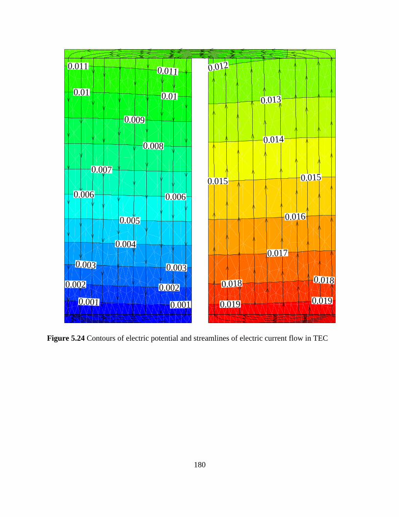
180

0.001 0.001

0.002 0.002

0.003 0.003

0.004

0.005

0.006 0.006

0.007

0.008

0.009

0.01 0.01

0.011 0.011 0.012

0.013

0.014

0.015 0.015

0.016

0.017

0.018 0.018

0.019 0.019

Figure 5.24 Contours of electric potential and streamlines of electric current flow in TEC

181

Field plots in Figs. 5.25 to 5.28 show temperature profile and streamlines of heat flow. Figures

5.25, 5.26, 5.27, and 5.28 represent four different cases of the effective thermal conductivities

with no particles, particle volume fraction 0.8 with Maxwell model, particle volume fraction 0.8

with Hasseman-Johnson model, and particle volume fraction 0.8 with Minnich-Chen model,

respectively. There is also a difference between the field plots in Figs. 5.26, 5.27, and 5.28 as

each field plot represents different effective transport property models. It can also be observed

that the temperature drop in a TE leg increases as the effective thermal conductivity decreases. A

low thermal conductivity decreases the heat conduction, which improves heat removal from the

cold surface of a TEC as demonstrated in Figs. 5.22 and 5.23. Temperature contours are linear in

Figs. 5.25, 5.26, and 5.27 but temperature contours show some non-linearity in Fig. 5.28. The

reason behind this could be very low thermal conductivity based on Minnich-Chen model and

generation of Joule heat.

182

290 290 290

291 291 291

292 292 292

293 293

294 294 294 294

295 295 295

296 296 296

297 297 297

298 298 298

299 299 299

Figure 5.25 Contours of temperature and streamlines of heat flow in TEC with cold surface

temperature 290 K, hot surface temperature 300 K, and electric potential 0.02 V with NO

particles

183

290 290 290

291 291 291

292 292 292

293 293

294 294 294 294

295 295 295

296 296 296

297 297 297

298 298 298

299 299 299


temperature 290 K, hot surface temperature 300 K, and electric potential 0.02 V with 0.8

volume fraction with Maxwell model

184

290 290 290 290

291 291291

292292 292

293293

294294 294

295 295295

296 296 296

297 297 297

298 298

299 299 299 299


temperature 290 K, hot surface temperature 300 K, and electric potential 0.02 V with 0.8 volume

fraction with Hasselman-Johnson model

185

290 290

290

291 291

291292 292

292293293294 294

294 294295 295 295296 296 296297 297 297298 298 298299 299


temperature 290 K, hot surface temperature 300 K, and electric potential 0.02 V with 0.8 volume

fraction with Minnich-Chen model

186

Figures 5.29 to 5.36 are for a composite TEG showing the temperature and electric potential

field plots. Figures 5.29 to 5.32 represent temperature which is marked by isothermal lines with

multi-colored background, while heat flow is presented by lines with arrows. Similarly, Figs.

5.33 to 5.36 represent electric potential which is indicated by marked iso-potential lines with a

multi-colored background, while electric current flow is indicated by lines with arrows.

Additionally, an external load with an electrical resistance similar to an internal resistance of

TEG is attached. Temperature contours show applied temperature gradient condition and the heat

flow direction. A change in temperature contour location is quite evident in the field plots as

shown in Figs. 5.29 to 5.32. Figures 5.29, 5.30, 5.31, and 5.32 represent TEG composite with no

particles, particle volume fraction of 0.8 with Maxwell model, particle volume fraction of 0.8

with Hasselman-Johnson model, and particle volume fraction of 0.8 with Minnich-Chen model,

respectively.

187

305 305 305 305

315 315 315

325 325 325

335 335

345 345 345

Figure 5.29 Contours of temperature and streamlines of heat flow in TEG with cold surface

temperature 300 K and hot surface temperature 350 K with NO particles

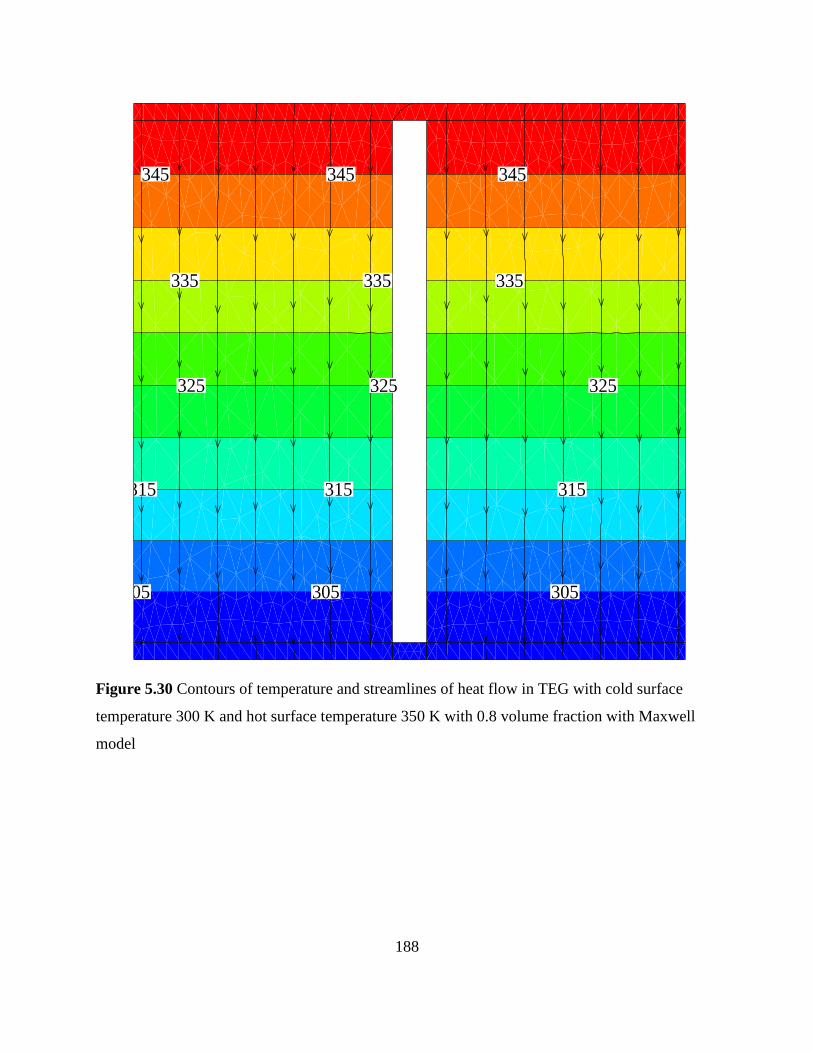
188

305 305 305

315 315 315

325 325 325

335 335 335

345 345 345


temperature 300 K and hot surface temperature 350 K with 0.8 volume fraction with Maxwell

model

189

305 305 305

315 315 315

325 325 325

335 335 335

345 345 345


temperature 300 K and hot surface temperature 350 K with 0.8 volume fraction Hasselman-

Johnson model

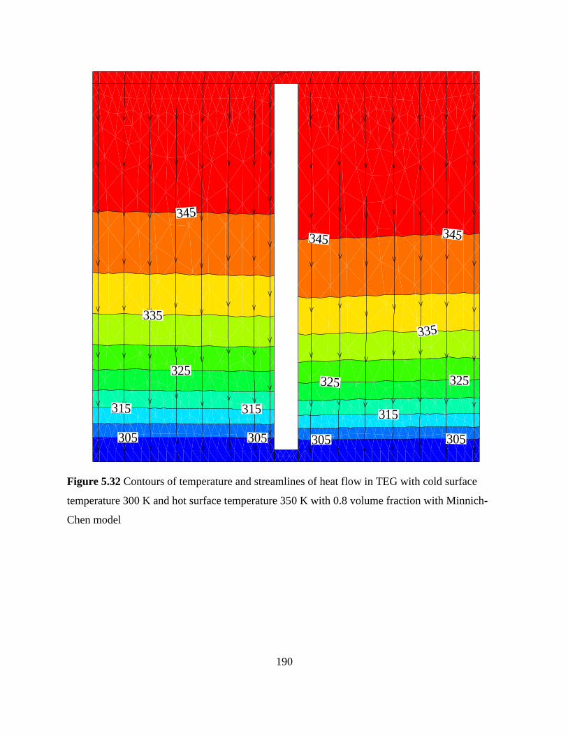
190

305 305 305 305

315 315 315

325325 325

335

335

345

345 345


temperature 300 K and hot surface temperature 350 K with 0.8 volume fraction with Minnich-

Chen model

191

Figures 5.33, 5.34, 5.35, and 5.36 presents the electric potential and current flow in TEG

composite with no particles, particle volume fraction of 0.8 with Maxwell model, particle

volume fraction of 0.8 with Hasselman-Johnson model, and particle volume fraction of 0.8 with

Minnich-Chen model, respectively. For a TEG, a low thermal conductivity can lower the amount

of heat absorbed from the heat source which brings down the heat input to TEG. A temperature

gradient to TEG remains unchanged so there is no change in the electric potential generation but

lower heat input increases the thermal efficiency of a TEG. Figures 5.34 to 5.36 show the

electrical potential generated due to the temperature gradient and flow of electric current. A

change in thermal conductivity shows no influence on electric potential because the effective

transport property models are only applied to thermal conductivity which only influences the

heat input.

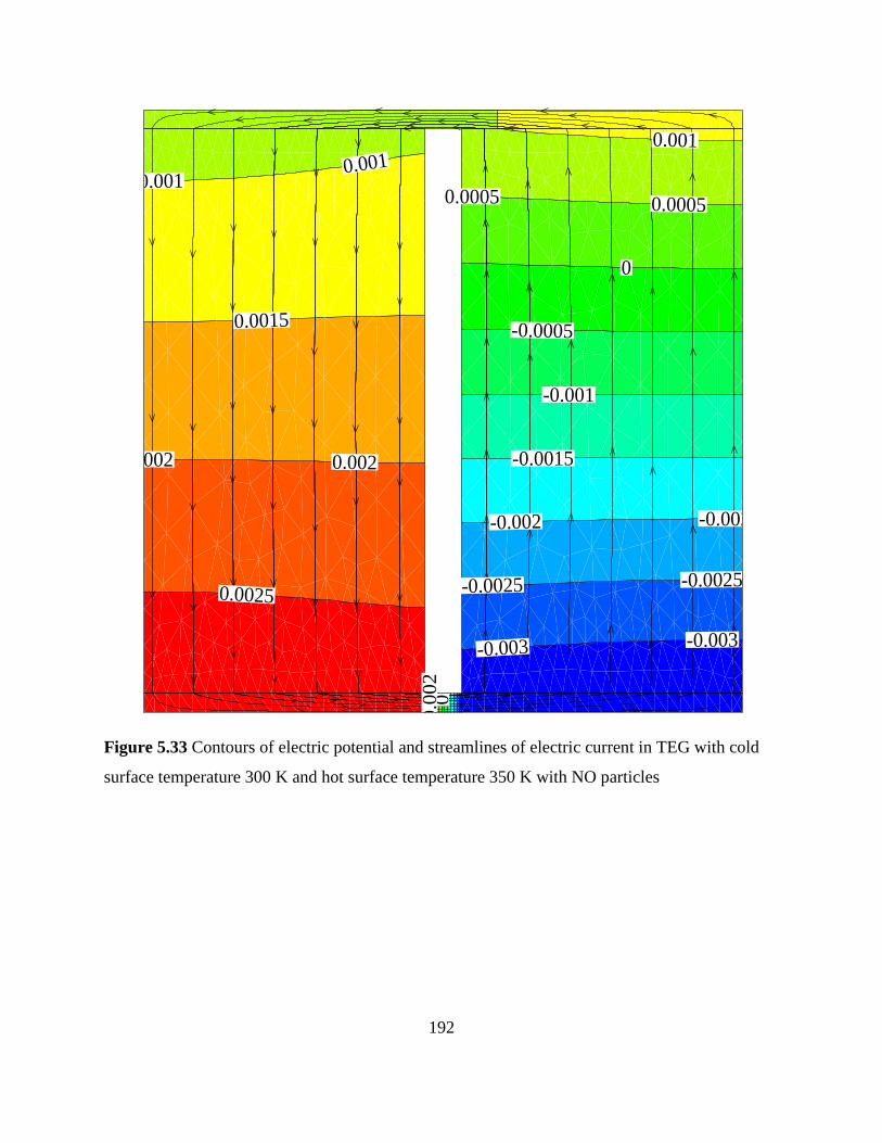
192

-0.003 -0.003

-0.0025 -0.0025

-0.002 -0.002

-0.0015

-0.001

-0.0005

0

0

0.0005 0.00050.001

0.0010.001

0.0015

0.002 0.002

0.0

02

0.0025

Figure 5.33 Contours of electric potential and streamlines of electric current in TEG with cold

surface temperature 300 K and hot surface temperature 350 K with NO particles

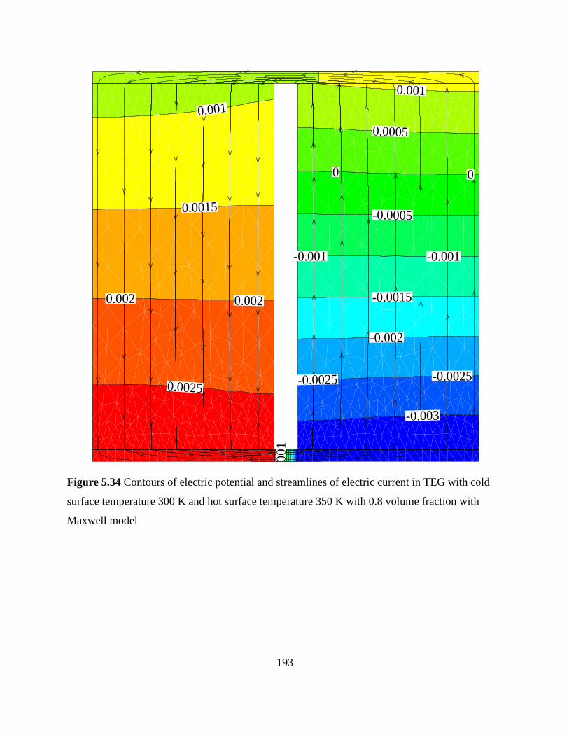
193

-0.003

-0.0025 -0.0025

-0.002

-0.0015

-0.001 -0.001

-0.0005

0 0

0.0005

0.001

0.0

01

0.001

0.0015

0.002 0.002

0.0025


surface temperature 300 K and hot surface temperature 350 K with 0.8 volume fraction with

Maxwell model

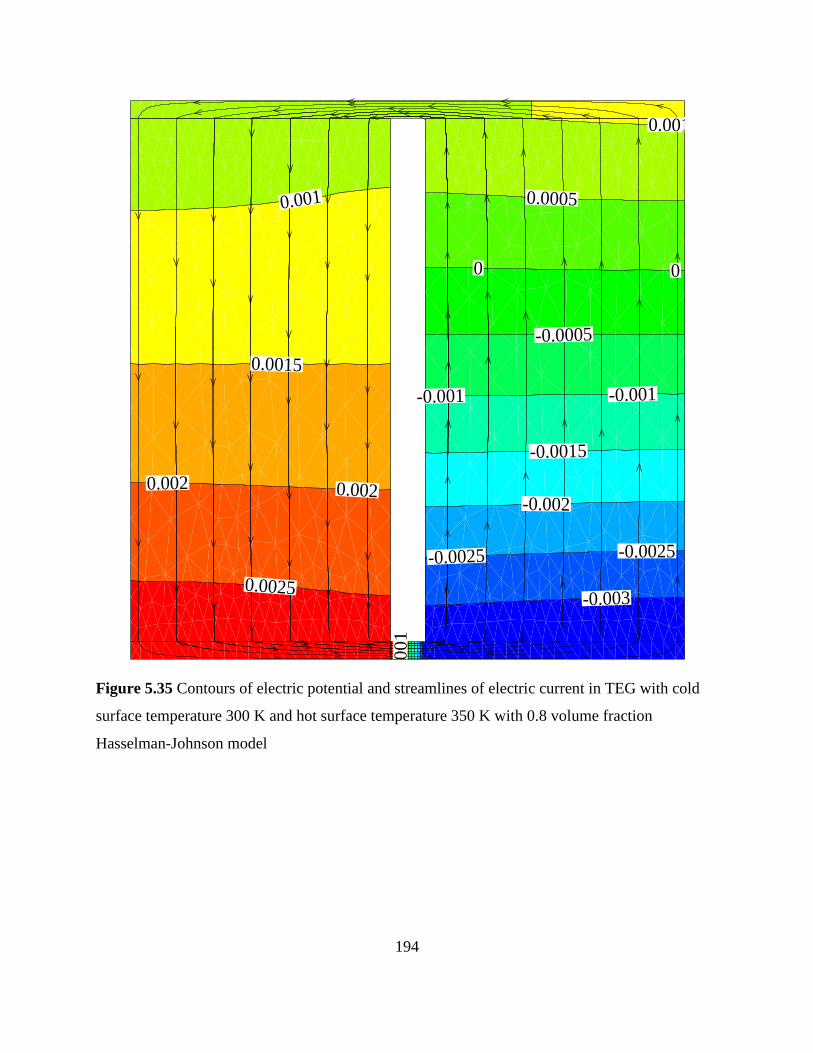
194

-0.003

-0.0025 -0.0025

-0.002

-0.0015

-0.001 -0.001

-0.0005

0 0

0.00050.001

0.0

01

0.001

0.0015

0.002 0.002

0.0025


surface temperature 300 K and hot surface temperature 350 K with 0.8 volume fraction


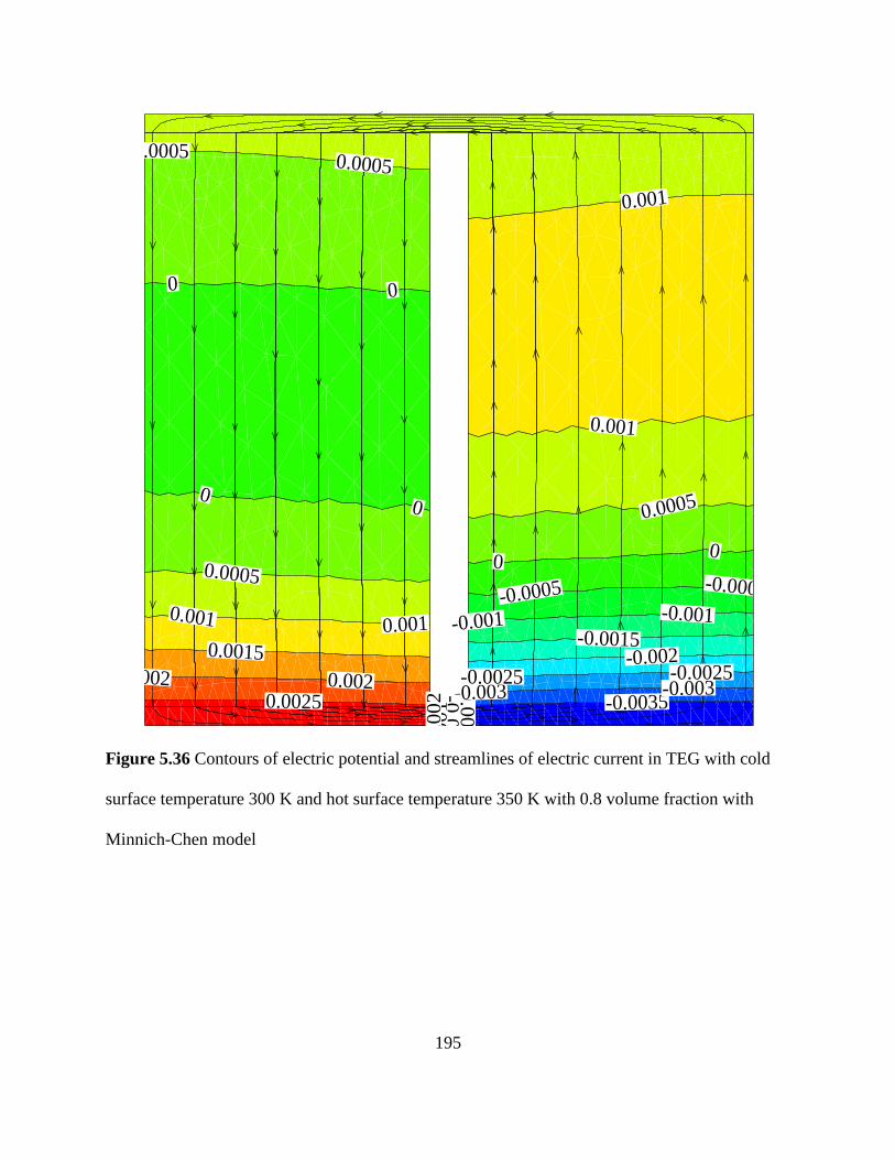
195

-0.0

03

5

-0.0035-0.003 -0.003-0.0025 -0.0025

-0.002-0.0015

-0.0

01

-0.001 -0.001-0.0005 -0.0005

00

0 0

00

0.00050.0005

0.0005

0.0005

0.001 0.001

0.0

01

0.001

0.001

0.00150.002 0.002

0.0

020.0025


surface temperature 300 K and hot surface temperature 350 K with 0.8 volume fraction with

Minnich-Chen model

196

Figures 5.37 and 5.38 are the comparisons between the analytical and numerical simulation

results. It can be observed from the plots that analytical results and numerical simulation show a

fair agreement. Nevertheless, analytical results overestimate results compared to the numerical

simulation due to decoupling between TE constitutive equations in analytical modeling. One can

also observe from plots that all effective transport property models predict same results when

particle volume fraction is zero.

197

Analytical results - Hasselman-Johnson model

Numerical simulation - Hasselman-Johnson model

Numerical simulation - Maxwell model

Analytical results - Maxwell model

CO

P

0 0.2 0.4 0.6 0.81.4

1.6

1.8

2

2.2

2.4

2.6

2.8

3

3.2

Analytical results - Minnich-Chen model

Numerical simulalation - Minnich-Chen model

Figure 5.37 Comparison of analytical and numerical simulation results for TEC

198

Analytical results - Minnich-Chen model

Numerical simulation - Minnich-Chen model

(%

)

0 0.2 0.4 0.6 0.80

1

2

3

4

5

6

7

8

9Analytical results - Maxwell model

Numerical simulation -- Maxwell model

Numerical simulation - Hasselman-Johnson model

Analytical results - Hasselman-Johnson model

Figure 5.38 Comparison of analytical and numerical simulation results for TEG

199

5.4 Conclusion

In this work, different effective transport property models based on the EMT were applied to

investigate the performance of a TEG and TEC. A one-dimensional (1-D) analytical heat transfer

model of a TEG and TEC was derived considering the Seebeck, Peltier, and Thomson effects,

Fourier heat conduction, Joule heating, and convection heat transfer. The performance of a TEC

and TEG are evaluated in terms of COP and thermal efficiency as a function of input electric

currents and temperature gradients, respectively. Additionally, the performance of a TEC and

TEG are also evaluated with respect to volume fractions of particles inside a composite TE leg.

The following conclusions are based on the studies:

1. The effective transport property models predict the decrease in the effective thermal

conductivity of composite TE materials. The composite TE materials are bulk materials and

easy to integrate in the real world applications.

2. A reduction in the effective thermal conductivity is favorable to the performance of a TEG

and TEC. COP and thermal efficiency increases as the effective thermal conductivity of

composite TE leg decreases.

3. This study shows that the heat conduction contribution to total heat input to a TEG and TEC

should remain as low as possible to increase the performance of a TEG and TEC. At this

stage, only way to decrease the heat conduction is reduction in thermal conductivity of TE

materials. Bulk TE composites provide economical and practical solution to decrease the

thermal conductivity.

200

5.5 Nomenclature


C volumetric specific heat (MJm-3

K-1

)

Cp specific heat (Jkg-1

K-1

)

D electric flux density (Nm2C

-1)

d depth (m)

E electric field intensity vector, (NC-1

)

h convection heat transfer coefficient, (Wm-2

K-1

)

H height (m)



)


K-1

)

K thermal boundary conductance (WK-1

m-2

)

L length (m)

1m A parameter (See Eq. (12))

2m A parameter (See Eq. (12))

n n-type material, number of particles

p p-type material

P Power input (W)


)

q heat (W)

.

q heat generation (Wm-3

)

Q heat (W)

r radius of sphere (m)

t time (s)

T temperature (K)

V electric potential (V)

W width (m)

ZT Figure of merit

201

Greek symbols


)

ε dielectric permittivity matrix (Fm-1

)

efficiency

thermal barrier resistance (KW-1

m-2

)

mean free path (Å)

electrical resistivity (Ω m), density (kgm-3

)


)

τ Thomson coefficient (VK-1

)

phonon group velocity (ms-1

)

volume fraction of particles

interface density (m-1

)

Subscripts

1 heat source, particle sphere

2 heat sink, base sphere


b base material

eff effective property

c composite, characteristic

conv convection

d gap distance

h hot temperature side

in input

l low temperature side

L Lattice contribution

m material

n n-type

out output

p particles, p-type

x co-ordinate system

202

CHAPTER 6: ANALYSIS OF COMBINED SOLAR PHOTOVOLTAIC-

NANOSTRUCTURED THERMOELECTRIC GENERATOR SYSTEM

6.1 Introduction

Currently, most of the power generation technologies use fossil fuels. Harmful emissions of

fossil fuels have forced to develop cost-effective power generation systems based on the

renewable energy conversion devices such as fuel cell, solar photovoltaic (PV) panel, solar-

thermal power generator, geothermal heat engine, and wind turbine. A direct power generation

technique using photovoltaic (PV) panels has been studied widely due to the huge availability of

solar energy. Solar PV panels are still less efficient and energy generated is expensive compared

to conventional energy conversion technologies. Although, different techniques have been used

(e.g., solar concentrators) to increase the efficiency of PV panels which increases the intensity of

solar radiation. The use of solar concentrators generates the higher PV cell temperature due to

higher irradiation on a solar PV panel which decreases the efficiency of solar panels (Dincer and

Meral 2010). Nevertheless, passive and active cooling methods (e.g., PV-thermal collectors) can

overcome the problem of higher cell temperature where waste heat is rejected to the environment

(Royne, Dey and Mills 2005). An option that remains largely unexplored is the use of

thermoelectric (TE) generator as a waste heat recovery tool in solar panels. A typical TE module

is made up of a number of p type and n type semiconductor legs connected electrically in

series and thermally in parallel. A TE module generates a voltage potential in the presence of an

applied temperature gradient across the module (Hoods 2005). The solar TE energy conversion

systems, where solar energy creates the temperature difference and produces electrical power

directly from the heat without moving parts has been discussed widely (Lenoir et al. 2003; Omer

and Infield 1998; Xi, Luo, and Fraisse 2007; Sahin et al. 2011). Shanmugam et al. (2011) have

developed the mathematical model of a TE generator system driven by the solar parabolic dish

collector. Their experiments found a maximum power output of 14.7 W with the solar radiation

ranges from 300 W/m2 to 1200 W/m

2. Chen (2011) has developed a mathematical model of a

solar TE generator considering an optical concentrator and selective surface. Chen (2011)

proposed a novel TE generator with an evacuated environment and concluded that such

arrangement can have attractive efficiency with 32TeBi TE materials and temperature ranges

203

from 150 ˚C to 250 ˚C. Khattab and Shenaway (2006) have proposed the use of a TE generator

to drive the TE cooler and optimized number of TE modules to achieve the maximum cooling

from one TE couple. Baranowski, Snyder and Toberer (2012) have developed a model for a solar

TE generator which can provide the analytical solutions of the device efficiency with

temperature dependant properties. They have also showed that with currently available materials,

total efficiency of 14.1% is possible for the cold and hot side temperature settings of 100 ˚C and

1000 ˚C, respectively. They also observed that the system efficiency can reach up to 25% if

figure of merit ( ZT ) reaches to 2 for the cold and hot side temperature settings of 100 ˚C and

1000 ˚C, respectively. Vatcharasathien et al. (2005) have developed a design methodology for a

solar TE power generation plant using TRANSYS software. Their simulation and experimental

work did not show the high performance but it demonstrated feasibility of power generation. Li

et al. (2010) have carried out experiments on three different types of TE generators (Bismuth-

Telluride, Skutterudite, and Silver-Antimony-Lead-Telluride) using the concentrated solar

energy. Li et al. (2010) have concluded that the conversion efficiency of a TE generator

increases with the increase in solar concentration ratio. Xiao et al. (2012) proposed three-stage

TE generator modules with medium temperature material (e.g., Skutterudite) and low

temperature material (e.g, Bismuth-Telluride). They achieved the efficiency of 10.52 %.

Vorobiev et al. (2006) have proposed a thermal-PV-solar hybrid system consisting of

concentrator, PV cell, and TE module. They concluded that TE modules can have considerable

effect on the overall efficiency of the thermal-PV-solar hybrid system. Rockendorf et al. (1999)

have studied a solar-PV-TE hybrid system with liquid heat-transfer medium and showed that

efficient back side cooling and low radiative losses can help achieving electrical conversion

efficiency up to 30% of the Carnot efficiency. Muhtaroglu, Yokochi, and Von Jouanne (2008)

demonstrated the use of PV and TE as a power source for mobile computing devices. They

showed an effective management of PV and TE simultaneously for onboard power generation

and concluded that such arrangement can extend battery life of mobile computing devices. Najafi

and Woodbury (2013) have developed combined PV-TE generator heat transfer model using

MATLAB. The hot surface of the TE module is considered in contact with air channel which is

in contact with the back surface of the PV panel. Najafi and Woodbury (2013) concluded that the

efficient TE modules can lead to a better power output of a combined system.

204

Performance of TE materials are characterised by a dimensionless parameter ‘figure of

merit’, TkZT )( 2 , where is the Seebeck coefficient, is the electrical resistivity, and k

is the thermal conductivity. Based on the available literature (Vineis et al. 2010), the ZT value of

the best available TE materials reach around 1 at room temperature. Recent advancement in

nanotechnology (Vineis et al. 2010) opens the door for further improvements of ZT for the TE

materials. The expression of the figure of merit, TkZT )( 2 , clearly indicates that one of the

methods to increase figure of merit is to reduce the thermal conductivity of the TE material.

Thermal conductivity has two components: the lattice conductivity Lk and electronic

conductivity ek (Godart et al. 2009). The electronic part of thermal conductivity ek is related

to the electrical conductivity using Wiedemann-Franz law (Godart et al. 2009) as shown in Eq.

(1),

TLke 0 (1)

where, 0L is the Lorentz number and for metals it is equal to (Godart et al. 2009),

8

2

22

0 1045.23

e

L

V2K

-2 (2)

where, is the Boltzmann constant (= 231038.1 JK-1

) and e is the electron charge

(= 191060.1 C)(Godart et al. 2009). The expression of figure of merit can be written in terms

of Lattice conductivity Lk and electronic conductivity ek as shown below (Godart et al.

2009),

Le

e

kk

k

LZT

0

2

. (3)

One method to enhance ZT is the inclusion of nanoparticles into the bulk TE materials which

can lead to low lattice thermal conductivity (Ma, Heijl, and Palmqvist 2013). Poudel et al. (2008)

achieved ZT value of 1.4 at 373 K by hot-pressing of nanopowders of 32TeBi and 32TeSb under

Argon Ar atmosphere. The enhanced ZT was attributed to significant decrease in lattice

thermal conductivity of material. Li et al. (2009) obtained ZT of 1.43 for double-doped 124SbCo

skutturedites using Indium In and Cerium Ce doping. The attractive results achieved using

nanotechnology has encouraged researchers to include nanoparticle-doped TE materials for

205

various applications, such as, solar TE generator and waste heat recovery. Kraemer et al. (2011)

have proposed novel solar TE generator with glass vacuum enclosure considering nanostructured

TE materials. The developed solar TE generator achieved maximum efficiency of 4.6% with

solar flux of 1000 Wm-2

condition. McEnaney et al. (2011) developed a novel of TE generator.

They placed high performance nanostructured material in evacuated tube with selective absorber

and achieved an efficiency of 5.2%.

It can be seen from the above discussion that the existing literature on the solar PV–nanomaterial

doped TE generator is very limited which is the major motivating factor to conduct the current

research. A combined system, which includes a solar PV and nano-particle doped TE modules, is

analyzed in this work. The temperature dependent thermophysical and electrical properties of TE

material, surface to surrounding convection heat transfer losses, and Thomson effect are included

in the current model. The energy transport in the solar PV panel and nanomaterial doped TE

module are performed separately and then combined to obtain a general expression of the overall

system.

6.2 Modeling and boundary conditions

The proposed photovoltaic – thermoelectric (PVTE) system is shown in Fig. 6.1a. A portion of

the heat rejected by PV panel will act as a heat source for the TE module. A number of

nanostructured p type and n type elements of the TE module are connected in series through

a copper plate with thermally conductive and electrically insulated ceramic plate on both sides.

In the current study, TE modules are placed in such a way that the ceramic plates of the modules

are attached to the back surface of the PV panel and exposed to the ambient environment,

respectively. For simplicity, a unit TE module with the copper plate is shown in Fig. 6.1b with

geometric dimension, a co-ordinate system, directions of different heat components, and thermal

boundary conditions. The PV panel has length PVl , width PVw and thickness PVt . A TE module

has length TEl , width TEw , and operates between the high and low temperature reservoirs bsT and

ambT , respectively. The TE module absorbs hQ amount of heat from the back surface of the PV

panel and rejects cQ amount of heat to the surrounding environment. The main mode of heat

206

transfer through PV-TE system is conduction. In addition to this, it is accompanied by

convection, radiation losses to surroundings from PV panel and internal heat generation, Peltier

heat generation/liberation at the junctions as well as Thomson heat generation in the TE module.

Convection heat loss from the side walls of a TE module to the surrounding environment is also

taken into account. Following section presents a mathematical model of the heat transfer for a

PV panel and TE module.

Modeling of PV system

Following assumptions are considered during the heat transfer modeling of a PV panel (Tiwari et

al. 2006):

The system is in quasi-steady state.

Transmittivity of ethylene vinyl acetate material (EVA) is nearly 100%.

Thermal resistance assumed to be negligible along the width of the PV panel considering

various layers such as glass, EVA, solar cells and tedlar.

The ethylene vinyl acetate (EVA) is used for encapsulation of photovoltaic modules due to their

good optical transmissivity, good electric insulator, and low water absorption ratio and tedlar is

polyvinyl fluoride film used for the back surface protection (Stark and Jaunich, 2011). The

different layers of solar PV panel are as shown in Fig. 6.2.

207

Figure 6.1 Schematic diagram of (a) photovoltaic – thermoelectric (PVTE) system and (b) unit

thermoelectric generator

Figure 6.2 Exploded view of Solar PV panel layers (Amrani 2007)

x

wTE

p n

Rl

Tbs

Tamb

I

Qconv

(a) (b)

Qh

Qc

Solar PV panel

TE Generator

Solar Radiation

Glass

Cover

Ethylene

Vinyl

Acetate

(EVA)

Ethylene

Vinyl

Acetate

(EVA)

Tedlar

Silicon Cells

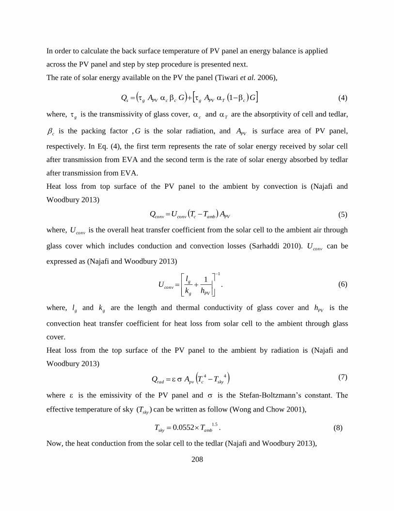
208

In order to calculate the back surface temperature of PV panel an energy balance is applied

across the PV panel and step by step procedure is presented next.

The rate of solar energy available on the PV the panel (Tiwari et al. 2006),

GAGAQ cTPVgccPVgs 1 (4)

where, g is the transmissivity of glass cover, c and T are the absorptivity of cell and tedlar,

c is the packing factor , G is the solar radiation, and PVA is surface area of PV panel,

respectively. In Eq. (4), the first term represents the rate of solar energy received by solar cell

after transmission from EVA and the second term is the rate of solar energy absorbed by tedlar

after transmission from EVA.

Heat loss from top surface of the PV panel to the ambient by convection is (Najafi and

Woodbury 2013)

PVambcconvconv ATTUQ (5)

where, convU is the overall heat transfer coefficient from the solar cell to the ambient air through

glass cover which includes conduction and convection losses (Sarhaddi 2010). convU can be

expressed as (Najafi and Woodbury 2013)

1

1

PVg

g

convhk

lU . (6)

where, gl and gk are the length and thermal conductivity of glass cover and PVh is the

convection heat transfer coefficient for heat loss from solar cell to the ambient through glass

cover.

Heat loss from the top surface of the PV panel to the ambient by radiation is (Najafi and

Woodbury 2013)

44

skycpvrad TTAQ (7)

where is the emissivity of the PV panel and is the Stefan-Boltzmann’s constant. The

effective temperature of sky )( skyT can be written as follow (Wong and Chow 2001),

5.10552.0 ambsky TT . (8)

Now, the heat conduction from the solar cell to the tedlar (Najafi and Woodbury 2013),

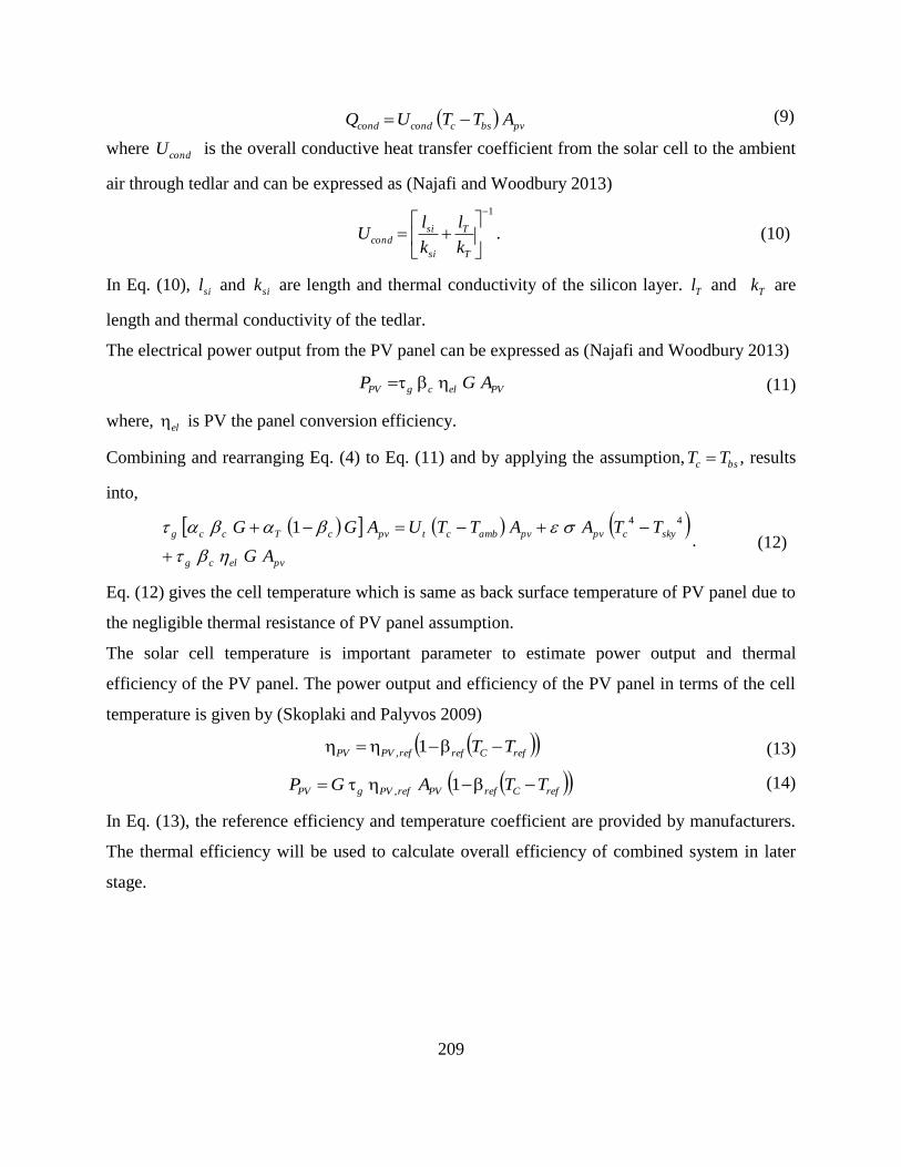
209

pvbsccondcond ATTUQ (9)

where condU is the overall conductive heat transfer coefficient from the solar cell to the ambient

air through tedlar and can be expressed as (Najafi and Woodbury 2013)

1

T

T

si

sicond

k

l

k

lU . (10)

In Eq. (10), sil and sik are length and thermal conductivity of the silicon layer. Tl and Tk are

length and thermal conductivity of the tedlar.

The electrical power output from the PV panel can be expressed as (Najafi and Woodbury 2013)

PVelcgPV AGP (11)

where, el is PV the panel conversion efficiency.

Combining and rearranging Eq. (4) to Eq. (11) and by applying the assumption, bsc TT , results

into,

pvelcg

skycpvpvambctpvcTccg

AG

TTAATTUAGG

44

1. (12)

Eq. (12) gives the cell temperature which is same as back surface temperature of PV panel due to

the negligible thermal resistance of PV panel assumption.

The solar cell temperature is important parameter to estimate power output and thermal

efficiency of the PV panel. The power output and efficiency of the PV panel in terms of the cell

temperature is given by (Skoplaki and Palyvos 2009)

refCrefrefPVPV TT 1, (13)

refCrefPVrefPVgPV TTAGP 1, (14)

In Eq. (13), the reference efficiency and temperature coefficient are provided by manufacturers.

The thermal efficiency will be used to calculate overall efficiency of combined system in later

stage.

210

Modeling of TE system

Heat transfer modeling of the TE effect has been carried out in this section. Following

assumption were made during the derivation of the heat transfer model for a TE system:

Isotropic and homogeneous material properties.

Thermal and electrical contact resistances were assumed negligible.

The energy transport equation inside a nanostructured TE module can be expressed as (Antonova

and Looman 2005):

genm qt

TC

q (15)

where symbols m , pC , T , q , and genq represent material density, specific heat, temperature,

heat generation rate per unit volume, and heat flux vector, respectively. The continuity of the

electric charge through the system must satisfy (Antonova and Looman 2005)

0

t

DJ (16)


respectively. Equation (15) and Eq. (16) are coupled by the set of TE constitutive equations

(Antonova and Looman 2005) as shown in Eq. (17) and Eq. (18) below

TkT ][][ Jq

)][(][ T EJ

(17)

(18)

where ][ is the Seebeck coefficient matrix, ][k is the thermal conductivity matrix, ][ is the


expressed as , where is the electric scalar potential (Landau, Lifshitz, and Pitaevskii

1984). Combining Eq. (15) to Eq. (18), the coupled TE equations for energy and charge transfers

can be expressed as

JEJ

TkT

t

TCm ][][ (19)

and

0][][][][

Tt

(20)

211

where ][ is the dielectric permittivity matrix and JE represents Joule heat (Antonova and

Looman 2005). Note that the material-property matrices (e.g., ][ and ][k , etc.) are suitable for

non-homogeneous materials. These, material-property matrices become single-valued property in

case of homogeneous materials. Initially, a simplified 1-D version of above equations will be

solved to obtain close forms of analytical solutions.

For 1-D analytical heat transfer modeling, a TE generator with N number of nanostructured

p type and n type semiconductor modules are connected electrically in series and thermally

in parallel and the end terminals are connected with the load resistance lR as shown in Fig. 1b.

TE elements have length TEl , width TEw , and works between the high and low temperature

reservoirs bsT and ambT respectively. A TE module absorbs hQ amount of heat from the back

surface of PV panel and rejects cQ amount of heat to the surrounding environment. The main

mode of heat transfer through a nanostructured semiconductor leg is the conduction and it is

accompanied by an internal heat generation in the form of the Joule effect, Peltier heat

generation/liberation at the junctions as well as Thomson heat generation. Convection heat loss

from the side walls of p type and n type semiconductor legs to the ambient environment is

also taken into account. Assuming isotropic and homogeneous material properties and neglecting

the thermal and electrical contact resistances between the contact surfaces a one dimensional

heat transfer equation under a steady state condition for nanostructured p type and n type

semiconductor legs is given by,

0)(2

2

2

2

dx

dT

kA

ITT

kA

ph

kA

I

dx

Tdamb

TE (22)

In Eq. (22) the first term is the Fourier heat conduction, second term is the Joule heating, third

term is the convection heat transfer loss, and fourth term is the Thomson effect. Equation (22)

can be written in the following form

02

2

Tdx

dT

dx

Td (23)

212

where

kA

I ;

kA

PhTE ; 2

2

kA

I

kA

pTh ambTE . (24)

Equation (23) is a linear and non-homogeneous ordinary differential equation. The general

solution to Eq. (23) is

XDXDeCeCxT 21

21 . (25)

where

2

42

1

D ;

2

42

2

D . (26)

Applying thermal boundary conditions at the top surface ( bsTTx ,0 ) and the bottom surface

( ambTE TTlx , ) one can determine the constants, 1C and 2C , of Eq. (25) as given below:

)( 12

22

1tt

tt

LDLD

amb

LDLD

bs

ee

TeeTC

;

)( 12

11

2tt

tt

LDLD

amb

LDLD

bs

ee

TeeTC

. (27)

Finally, the temperature distribution inside the nanostructured semiconductor legs can be

approximated from

.)()(

2

12

11

1

12

22

xD

LDLD

amb

LDLD

bsxD

LDLD

amb

LDLD

bse

ee

TeeTe

ee

TeeTxT

tt

tt

tt

tt

(28)

Now, combining heat transfer within the nanostructured semiconductor leg with Peltier heat,

which occurs at the junctions, heat transfer in nanostructured TE generator from back surface of

solar panel to surrounding environment is given by

.22112211 nnnnnnppppppbsh DCDCAkDCDCAkTIQ (29)

Heat rejected by TE generator to surrounding environment is given by

.21

21

2211

2211

tntn

tptp

LD

nn

LD

nnnn

LD

pp

LD

ppppambc

eDCeDCAk

eDCeDCAkTIQ

(30)

The power output of single TE generator can be calculated as

lTE RIP 2 . (31)

where

li

chnp

RR

TTI

)()(. (32)

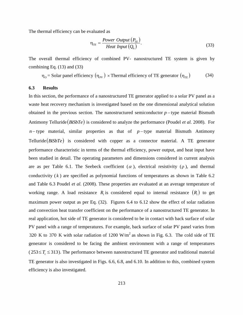
213

The thermal efficiency can be evaluated as

.h

TETE

QInputHeat

POutputPower

(33)

The overall thermal efficiency of combined PV- nanostructured TE system is given by

combining Eq. (13) and (33)

O = Solar panel efficiency PV Thermal efficiency of TE generator TE (34)

6.3 Results

In this section, the performance of a nanostructured TE generator applied to a solar PV panel as a

waste heat recovery mechanism is investigated based on the one dimensional analytical solution

obtained in the previous section. The nanostructured semiconductor p type material Bismuth

Antimony Telluride BiSbTe is considered to analyze the performance (Poudel et al. 2008). For

n type material, similar properties as that of p type material Bismuth Antimony

Telluride BiSbTe is considered with copper as a connector material. A TE generator

performance characteristic in terms of the thermal efficiency, power output, and heat input have

been studied in detail. The operating parameters and dimensions considered in current analysis

are as per Table 6.1. The Seebeck coefficient ( ), electrical resistivity ( ), and thermal

conductivity ( k ) are specified as polynomial functions of temperatures as shown in Table 6.2

and Table 6.3 Poudel et al. (2008). These properties are evaluated at an average temperature of

working range. A load resistance lR is considered equal to internal resistance iR to get

maximum power output as per Eq. (32). Figures 6.4 to 6.12 show the effect of solar radiation

and convection heat transfer coefficient on the performance of a nanostructured TE generator. In

real application, hot side of TE generator is considered to be in contact with back surface of solar

PV panel with a range of temperatures. For example, back surface of solar PV panel varies from

320 K to 370 K with solar radiation of 1200 W/m2

as shown in Fig. 6.3. The cold side of TE

generator is considered to be facing the ambient environment with a range of temperatures

( 313253 cT ). The performance between nanostructured TE generator and traditional material

TE generator is also investigated in Figs. 6.6, 6.8, and 6.10. In addition to this, combined system

efficiency is also investigated.

214

Table 6.1 Operating conditions and dimensional parameters of combined solar PVTE system

Parameter Value

Solar Radiation, G 0 to 1200

Convection heat transfer coefficient for TE generator, TEh 0 to 50

TE generator dimensions, TETETE twl 01.001.001.0

Solar PV panel dimensions, PVPVPV twl 05.011

Transmissivity of glass cover, g 0.95

Conductivity of glass cover, gk 1

Thickness of glass cover, gL 0.003

Absorptivity of solar cell, c 0.85

Packing factor, c 0.83

Absorptivity of tedlar, T 0.5

Reference thermal efficiency, refPV , 12%

Convection heat transfer coefficient for solar panel, PVh 5.8

Emissivity of solar PV panel, 0.88

Temperature coefficient, refPV , 0.0045

Reference Temperature, refT 25

215

Table 6.2 Polynomial functions of Seebeck coefficient, electrical conductivity, thermal

conductivity, and figure of merit with respect to temperature for nanostructured BiSbTe bulk

alloys (Poudel et al. 2008)

Property

(For n - type and

p -type material)

Temperature

range, (ºC)

Polynomial functions of different

thermoelectric

properties in terms of temperature

Seebeck

Coefficient,

2500 T 6

4936

23

1010738.710656.3

10732.2656.050.172

TT

TT

Electrical

Conductivity,

2500 T 5

41138

253

1010354.110093.2

10451.210575.8450.1

TT

TT

Thermal

Conductivity, k

2500 T

41037

254

10875.710809.3

10193.410946.2136.1

TT

TT

Figure of Merit, ZT 2500 T

4937

253

10149.110679.4

10765.110698.5034.1

TT

TT

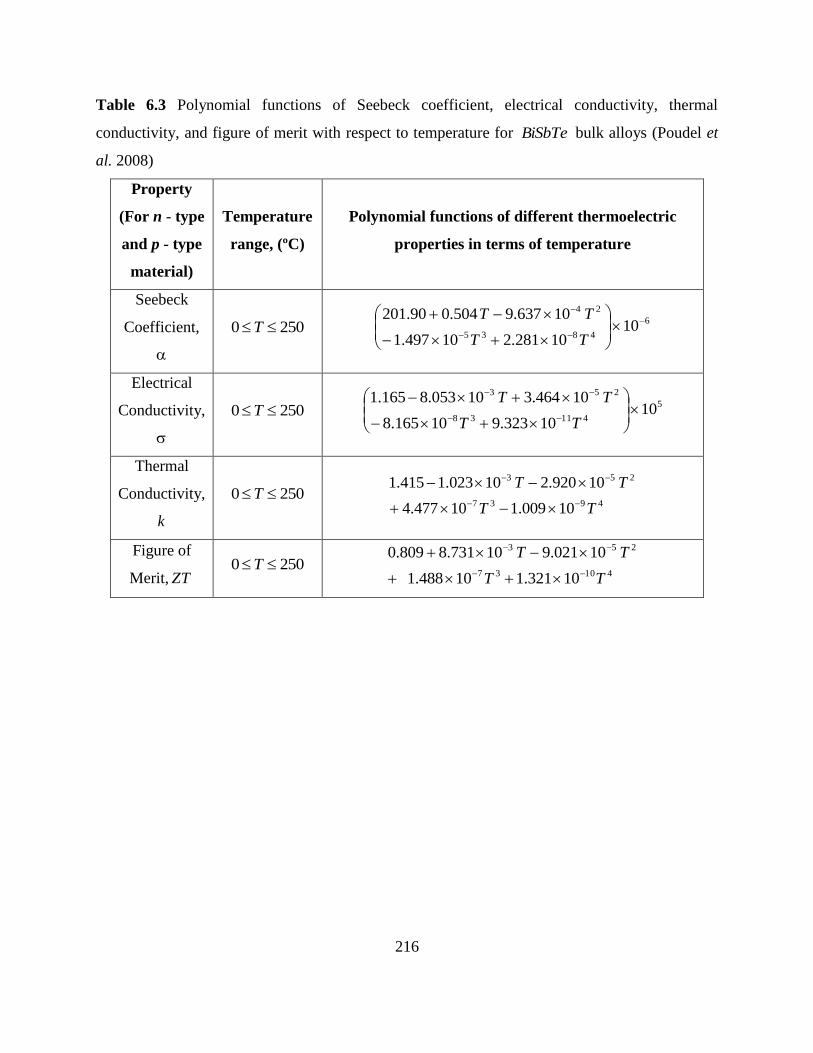
216

Table 6.3 Polynomial functions of Seebeck coefficient, electrical conductivity, thermal

conductivity, and figure of merit with respect to temperature for BiSbTe bulk alloys (Poudel et

al. 2008)

Property

(For n - type

and p - type

material)

Temperature

range, (ºC)

Polynomial functions of different thermoelectric

properties in terms of temperature

Seebeck

Coefficient,

2500 T 6

4835

24

1010281.210497.1

10637.9504.090.201

TT

TT

Electrical

Conductivity,

2500 T 5

41138

253

1010323.910165.8

10464.310053.8165.1

TT

TT

Thermal

Conductivity,

k

2500 T 4937

253

10009.110477.4

10920.210023.1415.1

TT

TT

Figure of

Merit, ZT 2500 T

41037

253

10321.110488.1

10021.910731.8809.0

TT

TT

217

The back surface temperature of a solar PV panel is an important parameter as TE generator is

considered to be attached directly beneath the solar PV panel. The back surface of the PV panel

acts as the heat source, bsT and the surrounding acts as the heat sink, ambT . The back surface

temperature is calculated using Eq. (12). The hot surface temperature bsT depends on the

surrounding temperature and solar radiation. The back surface temperature of a solar PV panel is

plotted as a function of solar radiation in Fig. 6.3 at different values of ambient temperature. It is

observed from Fig. 6.3 that an increase in the surrounding temperature increases the PV panel

back surface temperature. It is also observed from Fig. 6.3 that the PV panel’s back surface

temperature also increases with the increasing solar radiation. For example, PV panel back

surface temperature increases from 350 K to 358 K due to the increase in surrounding

temperature from 293 K to 303 K. For surrounding temperature 303 K, the PV panel back

surface temperature increases from 297 K to 358 K due to an increase in solar radiation from 0

W/m2 to 1200 W/m

2.

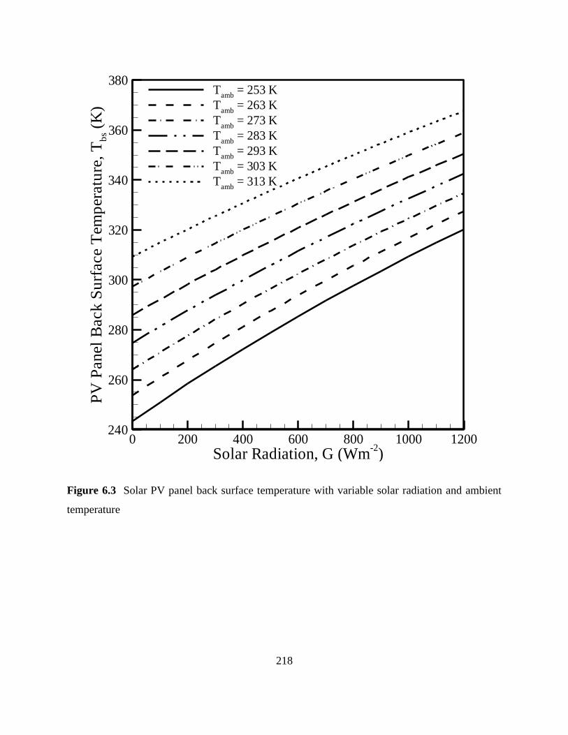
218

Solar Radiation, G (Wm-2

)

PV

Panel

Back

Su

rface

Tem

per

atu

re,

Tb

s(K

)

0 200 400 600 800 1000 1200240

260

280

300

320

340

360

380T

amb= 253 K

Tamb

= 263 K

Tamb

= 273 K

Tamb

= 283 K

Tamb

= 293 K

Tamb

= 303 K

Tamb

= 313 K

Figure 6.3 Solar PV panel back surface temperature with variable solar radiation and ambient

temperature

219

Figure 6.4 shows the temperature distribution along the length of p type and n type

nanostructured semiconductor legs. Equation (28) is used to calculate values of temperature as

presented in Fig. 6.4 for a specified hot surface temperature (356 K), surrounding temperature

(300 K), and different values of the convection heat transfer coefficients. It is observed from the

figure that the convection losses have larger impact on the temperature distribution along the

nanostructured thermoelectric legs. At higher values of the convection heat transfer coefficient

larger amount of heat was removed from the surface due to convection so that the temperature

drops more rapidly along the leg. It is shown later that convection affects the heat input to the

system and thermal efficiency of the system significantly.

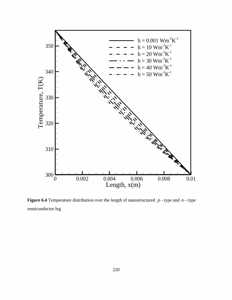
220

Length, x(m)

Tem

per

atu

re,T

(K)

0 0.002 0.004 0.006 0.008 0.01300

310

320

330

340

350h = 0.001 Wm

-2K

-1

h = 10 Wm-2

K-1

h = 20 Wm-2

K-1

h = 30 Wm-2K

-1

h = 40 Wm-2K

-1

h = 50 Wm-2

K-1

Figure 6.4 Temperature distribution over the length of nanostructured p type and n type

semiconductor leg

221

Effect of thermal energy input to the nanostructured thermoelectric system can be analysed from

Fig. 6.5. Heat input to the system is plotted as a function of the solar radiation at different values

of the convection heat transfer coefficients. Plot in Fig. 6.5 shows that with increase in the solar

radiation, more heat is available to convert. In addition, Fig. 6.5 also depicts the effect of

convection heat transfer coefficient. For a given solar radiation, with higher convection heat

transfer coefficient, heat input to the system increases. This establishes that due to higher

convection losses more heat is drawn from heat reservoir to the hot surface. Figure 6.6 shows the

heat input comparison between the traditional TE generator and nanostructured TE generator.

For the given range of input solar radiation, the magnitude of heat input to the TE system is

higher for a traditional TE generator compared to nanostructured TE generator. For example,

with solar radiation of 1200 W/m2 and adiabatic side-wall conditions, the heat available to

convert is 1.94 W for nanostructured TE generator and 2.13 W for traditional TE generator. This

can be attributed to the decrease in the thermal conductivity of a nanostructured TE material. As

shown in Fig. 6.7, traditional TE material has higher thermal conductivity so more amount of

heat is available for traditional TE generator than nanostructured TE generator.

222


)

Hea

tIn

pu

t,Q

h(W

)

200 400 600 800 1000 1200

0.5

1

1.5

2

2.5

3

h = 10-6

Wm-2

K-1

h = 10 Wm-2K

-1

h = 20 Wm-2K

-1

h = 30 Wm-2

K-1

h = 40 Wm-2

K-1

h = 50 Wm-2K

-1

Figure 6.5 Heat input to nanostructured TE generator with different solar radiation and variable

convection heat transfer coefficient

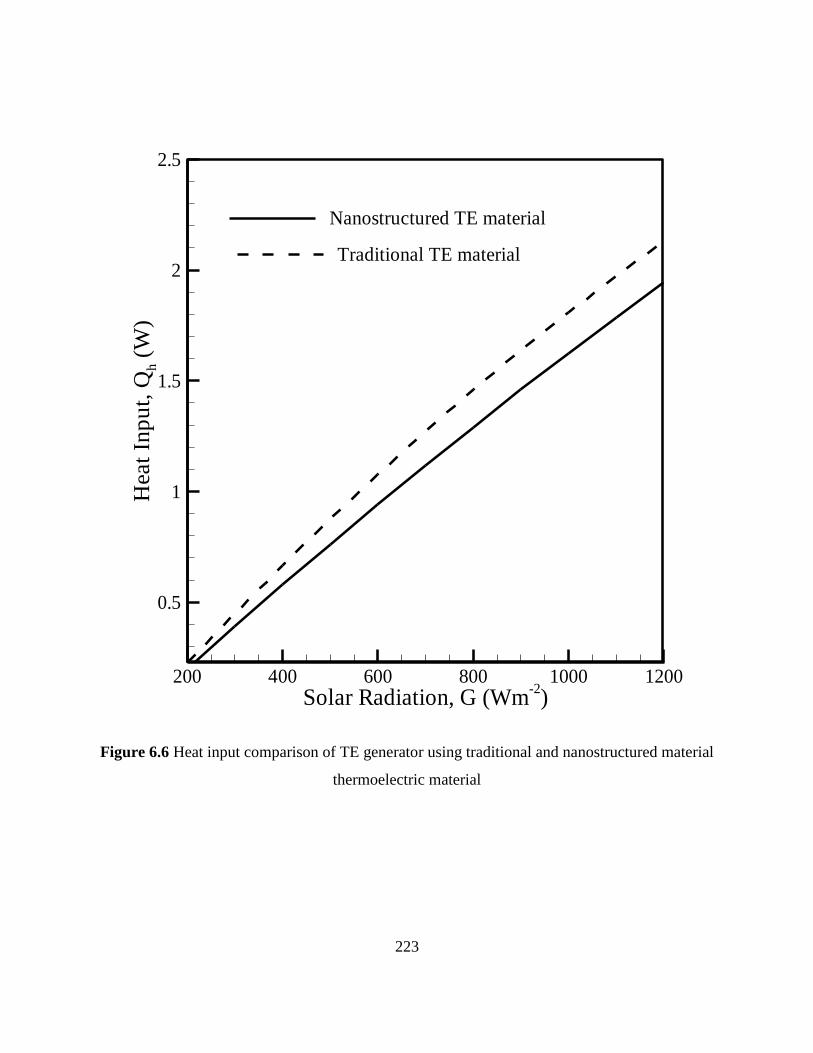
223

Traditional TE material


)

Hea

tIn

pu

t,Q

h(W

)

200 400 600 800 1000 1200

0.5

1

1.5

2

2.5

Nanostructured TE material

Figure 6.6 Heat input comparison of TE generator using traditional and nanostructured material

thermoelectric material

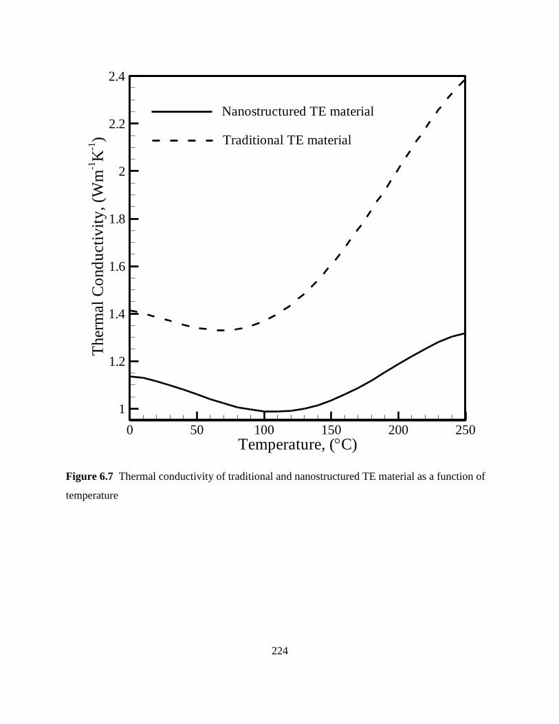
224

Temperature, (C)

Th

erm

al

Co

nd

ucti

vit

y,

(Wm

-1K

-1) Traditional TE material

0 50 100 150 200 250

1

1.2

1.4

1.6

1.8

2

2.2

2.4


Figure 6.7 Thermal conductivity of traditional and nanostructured TE material as a function of

temperature

225

Figure 6.8 demonstrates the power output of a TE generator as a function of solar radiation. As

the hot surface temperature increases due to increase in the solar radiation, power output also

increases. As one can analyse from Eq. (31) & (32), temperature difference has large impact on

the power output. In this case, the hot surface temperature depends largely on the solar radiation.

The same equation verifies that power output is independent of convection heat transfer losses. It

also shows power output comparison between the nanostructured and traditional TE generator.

An increment in the figure of merit due to the incorporation of nano-particle in the bulk material

matrix can be attributed to the surge in power output. The power output increases by 3% due to

the use of a nanostructured TE material with 1200 W/m2

input solar radiation condition.

226



)

Po

wer

Ou

tpu

t,P

o(W

)

200 400 600 800 1000 1200

0.01

0.02

0.03

0.04

0.05

0.06

0.07

Nanostructred TE material

Figure 6.8 Power output from TE generator as a function of solar radiation

227

Figure 6.9 also establishes the effect of the surface to surrounding convection heat transfer on the

thermal efficiency. For a given temperature difference between hot and cold surfaces, an increase

in the convection heat transfer coefficient decreases the thermal efficiency of a system.

Irreversible convection process cause the larger amount of heat loss to the ambient environment;

therefore, it suggests that less heat is available to generate electric potential and this leads to

lower thermal efficiency. Figure 6.10 shows a comparison between the thermal efficiency of a

TE generator using the traditional TE material and nanostructured TE material. The

nanostructured TE material improves the thermal efficiency of a TE generator from 3.09% to

3.47% i.e., 12% increment compared to traditional TE material.

228


)

Th

erm

al

Eff

icie

ncy

,

t(%

)

200 400 600 800 1000 1200

0.5

1

1.5

2

2.5

3

3.5

h = 10-6

Wm-2K

-1

h = 10 Wm-2

K-1

h = 20 Wm-2

K-1

h = 30 Wm-2K

-1

h = 40 Wm-2K

-1

h = 50 Wm-2

K-1

Figure 6.9 Thermal efficiency of nanostructured TE generator with different solar radiation and

variable convection heat transfer coefficient

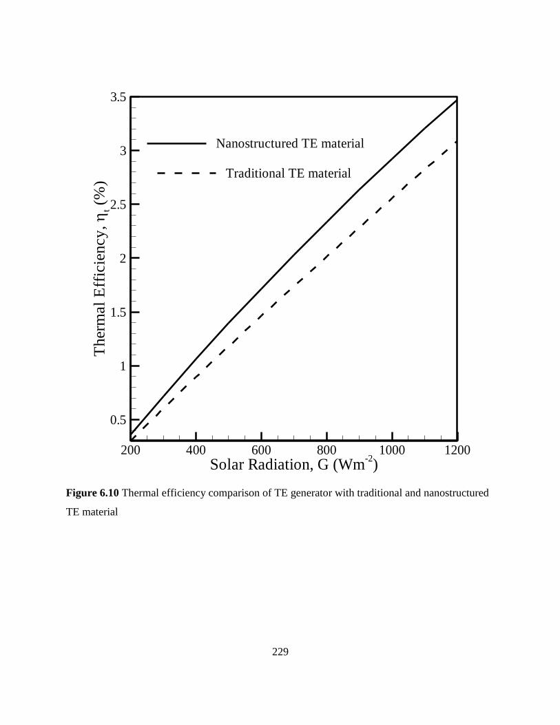
229



)

Th

erm

al

Eff

icie

ncy

,

t(%

)

200 400 600 800 1000 1200

0.5

1

1.5

2

2.5

3

3.5


Figure 6.10 Thermal efficiency comparison of TE generator with traditional and nanostructured

TE material

230

In order to compare the power output between the solar PV panel and TE generator, the back

surface of a PV panel is considered to be filled with TE modules. For example, for a plot in Fig.

6.11 a solar panel with surface area of 1 m2 is considered and back surface is covered with TE

generators with surface area 0.00025 m2 on its back surface. Theoretically the power output of

solar PV panel remains 100 W whereas TE generators reach up to 200 W of power output at

1200 W/m2.

231


)

Po

wer

Ou

tpu

t,P

o(W

)Solar Panel Output

200 400 600 800 1000 1200

50

100

150

200

TE Generator Output

Figure 6.11 Power output comparison of solar PV panel and TE generator

232

The solar panel efficiency is investigated by Eq. (13). The performance of a solar PV panel

deteriorates as the temperature rises, because efficiency of solar panel is a function of cell

temperature. Fig. 6.12 shows the downward trend in the thermal efficiency as intensity of solar

radiation rises. In contrary, the efficiency of a TE generator rises as solar radiation increases. Fig.

6.13 is a combined efficiency of a solar PV-TE system. The efficiency of a combined system

remains low during the low solar radiation because it does not generate high temperature

gradient. The efficiency of a TE generator increases as solar radiation increases and that

compensates the low efficiency of solar PV panel at higher solar radiation. For example, at solar

radiation of 500 W/m2 the efficiency of solar PV panel is 10.68% and it rises to 14.88% with

combined the solar PV-TE system. A TE generator has less impact on overall efficiency of

combined system at lower solar radiation but it has a large impact on thermal efficiency at the

higher solar radiation.

233

Solar Panel

Solar Radiation, G (Wm-2)

Th

erm

al

effi

cie

ncy

,t(%

)

200 400 600 800 1000 1200

1

2

3

4

5

6

7

8

9

10

11

12

TE generator

Figure 6.12 Solar panel conversion efficiency Vs. Solar Radiation

234


)

Co

mb

ined

effi

cie

ncy

,c

(%)

200 400 600 800 1000 1200

14

16

18

20

22

24

26

Figure 6.13 Combined efficiency of solar PVTE system Vs. Solar Radiation

235

6.4 Conclusion

In the present work, a combined solar PV-nanostructured TE power generation system is

proposed. TE modules are attached to the back surface of a solar PV panel to use the excess heat

of a PV panel. A heat transfer model of a solar PV panel and TE generator has been derived. A

one-dimensional (1-D) heat transfer model is derived involving the Fourier heat conduction,

Joule and convection losses, and Peltier, Seeback and Thomson effects. The temperature

dependent nanostructured thermoelectric properties have been considered for the analysis. The

influences of solar radiation and convection heat transfer coefficients on various performance

parameters of a nanostructured TE generator such as power output, heat input, and thermal

efficiency have been studied. In addition to this, the performance between nanostructured and

traditional TE material has been compared. The improved nanostructured TE material has

enhanced TE properties which are reflected in terms of better power output and thermal

efficiency. The higher electrical conductivity and lower thermal conductivity of nanostructured

TE materials are key reasons to increase the thermal efficiency and power output of a

nanostructured TE generator. Furthermore, the effect of a TE generator on combined system is

evaluated in terms of improved combined efficiency of the system. TE modules have a large

impact on the performance of a combined solar PV-TE system at the higher solar radiation.

236

6.5 Nomenclature


C specific heat capacity (kJkg-1

K-1

)

D electric flux density vector (Nm2C

-1)

e electron charge (C)


)

G solar irradiation (Wm-2

)


K-1

)



)


K-1

)

0L Lorentz number (V2K

-2)

l length (m)

N number of modules

p Perimeter (m)

P power output (W)


)

.


)

Q heat or energy (W)

R resistance )(

S entropy (Wm-3

K-1

)

t thickness (m), time (s0

T temperature (K)

U heat transfer coefficient (Wm-2

K-1

)

V voltage (V)

w width (m)

x coordinate (m)


absorptivity, Seebeck coefficient (VK-1

)

237

packing factor, temperature coefficient

emissivity of PV panel, dielectric permittivity (Fm-1

)

efficiency


a parameter (see Eq. (24)), temperature coefficient (K-1

)

electrical resistivity )(

m density (kgm-3

)

Boltzmann constant (JK-1

), electrical conductivity (Sm-1

)

Transmissivity, Thomson coefficient (VK-1

)



Subscripts

amb ambient

bs Solar panel back surface tempeature

c cell, cold side of thermoelectric module

cond conduction

conv convection

e electronic

el electrical

g glass cover

gen generation

h hot side of thermoelectric module

i internal

L Lattice

l External load

mp maximum powerpoint

n n type semiconductor material

o output, overall

p p type semiconductor material

238

PV solar PV panel

rad radiation

ref reference

s sun

si silicon

sky sky

T tedlar, thermal

TE thermoelectric module

239

CHAPTER 7: NANOSTRUCTURING OF n-type Bi2Te2.7Se0.3 BASED ON

SOLID STATE SYNTHESIS TECHNIQUE

7.1 Introduction

Thermoelectric (TE) energy conversion systems offer unique advantages of being silent in

operation, no moving parts, no refrigerants, robust in nature, and long service life. Nevertheless,

extremely low energy conversion efficiency limits TE systems from widespread real world

applications in power generation and cooling. TE systems are first choice of interest for power

generation and cooling/heating for extreme environments, such as deep space probes. The

performance of TE systems are measured based on Figure of Merit (ZT=α2σ/k) of TE materials.

For a good ZT, the power factor (α2σ) should be high and thermal conductivity (k) should be as

low as possible. The power factor improvement and the thermal conductivity reduction have

been achieved in different materials. Hicks and Dresselhaus (1993) discussed the concept of

quantum wire (one dimensional) for TE materials. ZT improvement in quantum wire is due to

increase in the power factor (α2σ) but not significantly due to the low thermal conductivity

(Hicks and Dresselhaus 1993). Another method to increase ZT was demonstrated experimentally

by Venkatasubramanian et al. (2001), where ZT of p-type superlattice of Bi2Te3/Sb2Te3

(bismuth-telluride-antimony) improved from 1 to 2.4 due to the reduction in the thermal

conductivity. Improvements offered by Hicks and Dresselhaus (1993) and Venkatasubramanian

et al. (2001) were primarily for the low dimensional structures, such as quantum dots, wires, and

superlattice structures. The low dimensional structures can be manufactured using different

methods, such as electroless etching (Hochbaum et al. 2008), Superlattice Nanowire Pattern

Transfer (SNAP) (Boukai et al. 2008), Chemical Vapor deposition (Venkatasubramanian et al.

1997), and Molecular-Beam Epitaxy (MBE) (Hicks et al. 1996). A low-dimensional structure

can be employed limitedly in the real world applications due to the complicated

physical/chemical vapor deposition method and cost of manufacturing (Ma et al. 2013). There is

another route to improve the ZT in bulk TE materials called ‘nanocomposite bulk materials’

(Bottner and Konig 2013). Nanocomposites can be manufactured using various methods which

are relatively less complicated compared to the low-dimensional methods. A 3D bulk composite

can be made with the combination of hot press, high energy ball milling, spark plasma sintering,

240

and solid state reaction (Nolas et al. 2000, Zhou et al. 2008, Poudel et al. 2008, He et al. 2006).

Figure 7.1 shows some of the ZT improvements in TE materials in low-dimensional and bulk

structures.

Figure 7.1 ZT improvements in low dimensional and bulk TE materials

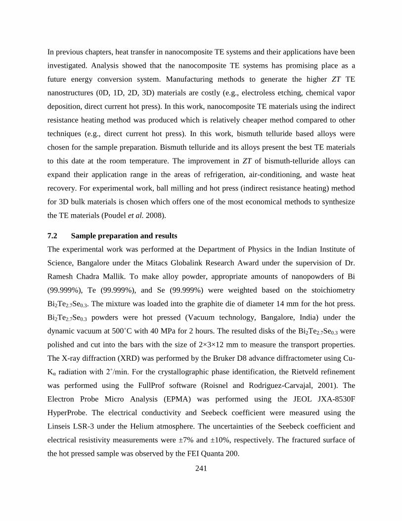
241

In previous chapters, heat transfer in nanocomposite TE systems and their applications have been

investigated. Analysis showed that the nanocomposite TE systems has promising place as a

future energy conversion system. Manufacturing methods to generate the higher ZT TE

nanostructures (0D, 1D, 2D, 3D) materials are costly (e.g., electroless etching, chemical vapor

deposition, direct current hot press). In this work, nanocomposite TE materials using the indirect

resistance heating method was produced which is relatively cheaper method compared to other

techniques (e.g., direct current hot press). In this work, bismuth telluride based alloys were

chosen for the sample preparation. Bismuth telluride and its alloys present the best TE materials

to this date at the room temperature. The improvement in ZT of bismuth-telluride alloys can

expand their application range in the areas of refrigeration, air-conditioning, and waste heat

recovery. For experimental work, ball milling and hot press (indirect resistance heating) method

for 3D bulk materials is chosen which offers one of the most economical methods to synthesize

the TE materials (Poudel et al. 2008).

7.2 Sample preparation and results

The experimental work was performed at the Department of Physics in the Indian Institute of

Science, Bangalore under the Mitacs Globalink Research Award under the supervision of Dr.

Ramesh Chadra Mallik. To make alloy powder, appropriate amounts of nanopowders of Bi

(99.999%), Te (99.999%), and Se (99.999%) were weighted based on the stoichiometry

Bi2Te2.7Se0.3. The mixture was loaded into the graphite die of diameter 14 mm for the hot press.

Bi2Te2.7Se0.3 powders were hot pressed (Vacuum technology, Bangalore, India) under the

dynamic vacuum at 500˚C with 40 MPa for 2 hours. The resulted disks of the Bi2Te2.7Se0.3 were

polished and cut into the bars with the size of 2×3×12 mm to measure the transport properties.

The X-ray diffraction (XRD) was performed by the Bruker D8 advance diffractometer using Cu-

Kα radiation with 2˚/min. For the crystallographic phase identification, the Rietveld refinement

was performed using the FullProf software (Roisnel and Rodriguez-Carvajal, 2001). The

Electron Probe Micro Analysis (EPMA) was performed using the JEOL JXA-8530F

HyperProbe. The electrical conductivity and Seebeck coefficient were measured using the

Linseis LSR-3 under the Helium atmosphere. The uncertainties of the Seebeck coefficient and

electrical resistivity measurements were ±7% and ±10%, respectively. The fractured surface of

the hot pressed sample was observed by the FEI Quanta 200.

242

Figure 7.2 presents the Rietveld refinement of the XRD pattern of powders. The XRD patterns

verify that the powder is in the single phase and well matched with Bi2Te2.7Se0.3. The peaks of

Bi2Te2.7Se0.3 were indexed with Bi2Te2.4Se0.6 (ICSD#617110).

Figure 7.2 Rietveld refinement powder XRD pattern for Bi2Te2.7Se0.3

243

Figures 7.3 to 7.5 present the transport properties of Bi2Te2.7Se0.3 and Sb1.5Bi0.5Te3. Figure 7.3

show the Seebeck coefficient and electrical resistivity of Bi2Te2.7Se0.3 as a function of

temperature. The Seebeck coefficient decreases and electrical resistivity increases as the

temperature rises. The power factor shows a decreasing trend in Figure 7.4 as temperature rises.

The highest power factor was observed 955 μWm-1

K-2

at 87 ˚C.

Temperature (C)

Seeb

eck

Co

eff

icie

nt

(V

K-1

)

50 100 150 200-176

-174

-172

-170

-168

-166

-164

Seebeck Coefficient

Ele

ctr

ical

Resi

stiv

ity

(m

m)

0.029

0.03

0.031

0.032

0.033

0.034

0.035

Electrical Resistivity

Figure 7.3 Seebeck coefficient and Electrical resistivity of sample Bi2Te2.7Se0.3

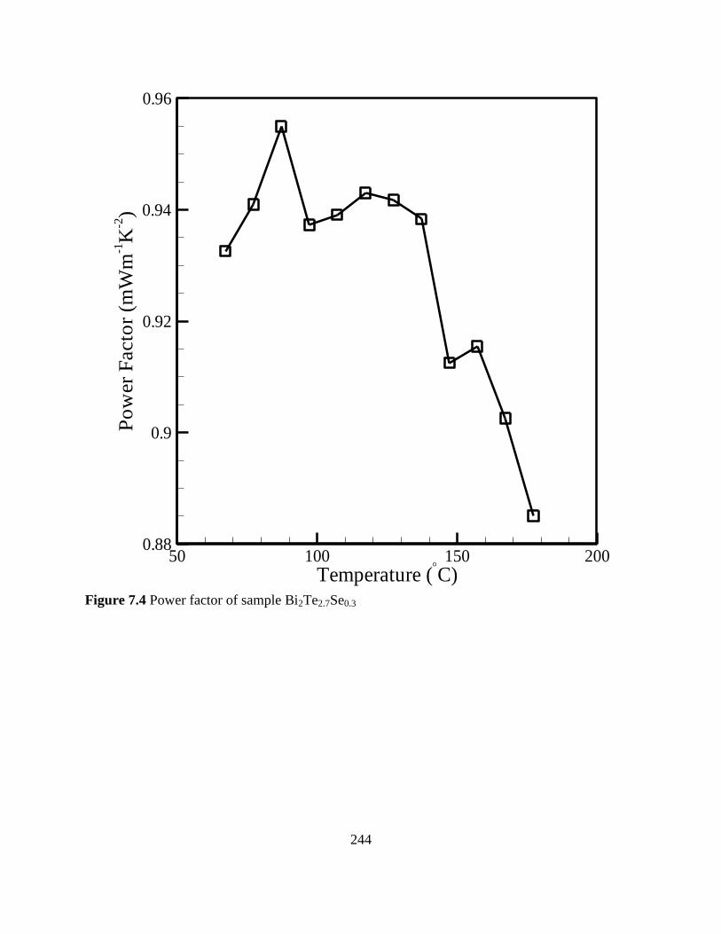
244

Temperature (C)

Po

wer

Facto

r(m

Wm

-1K

-2)

50 100 150 2000.88

0.9

0.92

0.94

0.96

Figure 7.4 Power factor of sample Bi2Te2.7Se0.3

245

Figure 7.5 presents a comparison between the power factors of Bi2Te2.7Se0.3 manufactured using

different hot press techniques. Yan et al. (2010) used the direct current hot press to synthesize

the Bi2Te2.7Se0.3 powder, whereas, the current work used the indirect resistance heating to

synthesize the Bi2Te2.7Se0.3 powder. One can observe from the plot that the power factor

increases rapidly for a similar temperature range when the direct current hot press is used. The

reason behind the low power factor can be randomness of the grains (Yan et al. 2010). The SEM

images in Figure 7.6 show those random grains without preferred crystal orientation.

Additionally, density of a sample turned out to be 84% which was measured using the

Archimedes’ principle. This lower density suggests that the sample was not compressed enough

due to the inadequate pressure and temperature.

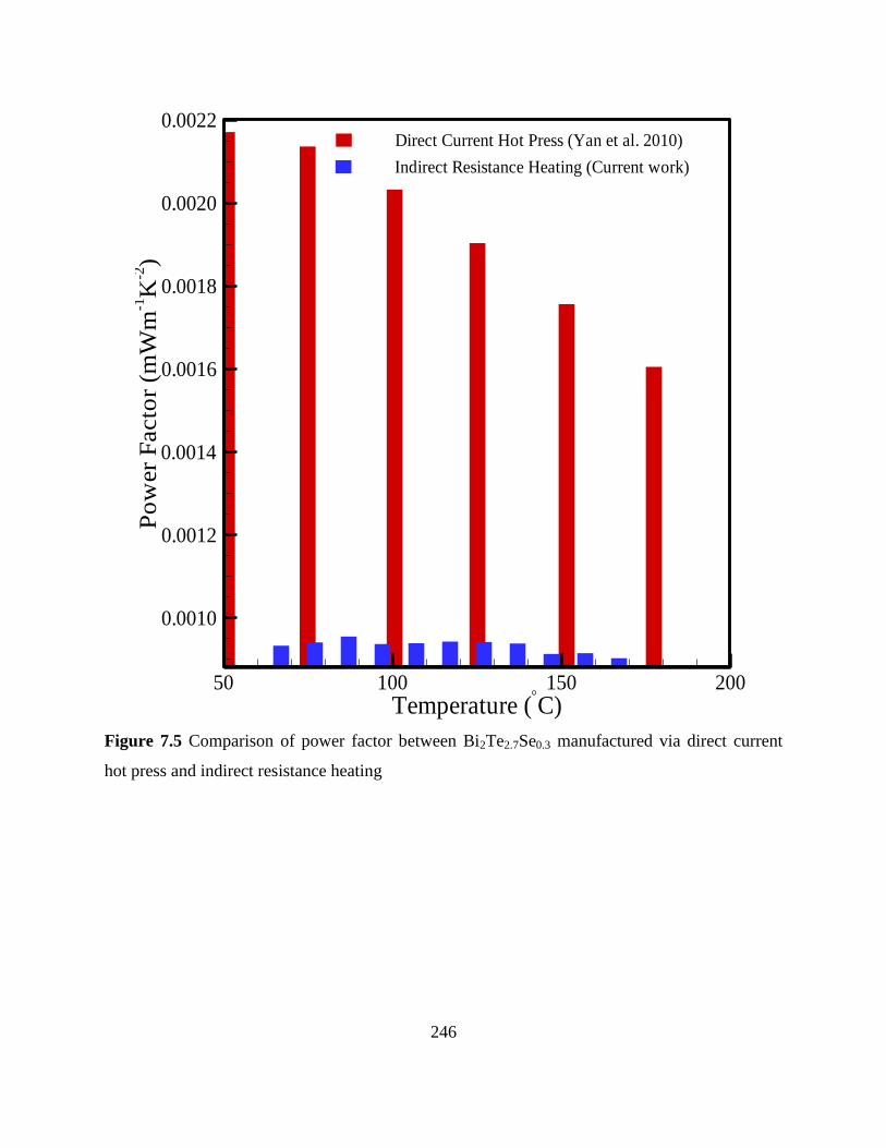
246

Temperature (C)

Po

wer

Facto

r(m

Wm

-1K

-2)

50 100 150 200

0.0010

0.0012

0.0014

0.0016

0.0018

0.0020

0.0022Direct Current Hot Press (Yan et al. 2010)

Indirect Resistance Heating (Current work)

Figure 7.5 Comparison of power factor between Bi2Te2.7Se0.3 manufactured via direct current

hot press and indirect resistance heating

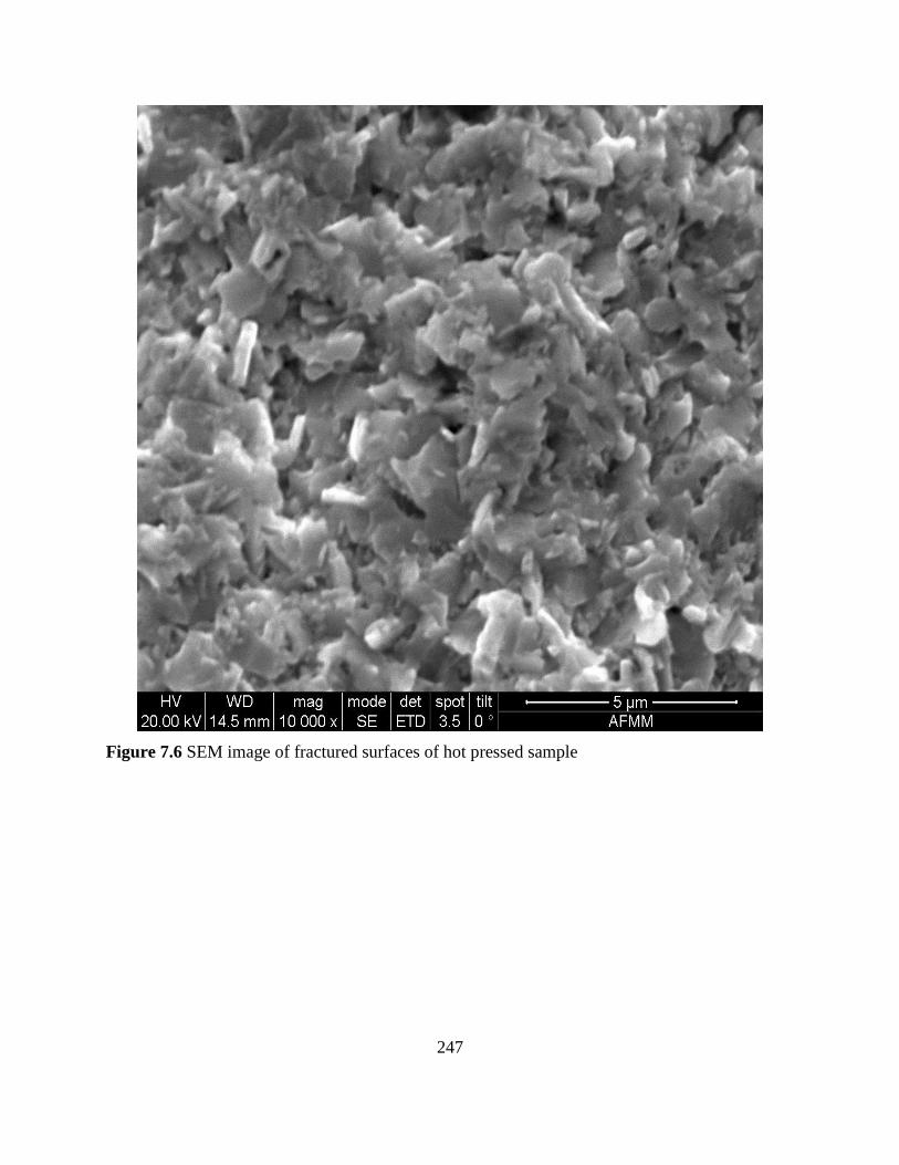
247

Figure 7.6 SEM image of fractured surfaces of hot pressed sample

248

7.3 Conclusion

In this work, Bi2Te2.7Se0.3 samples were prepared via ball milling and an indirect resistance

heating hot press. The power factor of hot-pressed Bi2Te2.7Se0.3 sample followed a decreasing

trend as the temperature increases. The grains in Bi2Te2.7Se0.3 were observed (via SEM image)

without preferred orientation which could have contributed to the higher electrical resistivity. An

indirect resistance heating hot press method provides an alternative economical route to make TE

legs, but the synthesized bulk TE legs do not exhibit the high power factor which can reduce the

ZT. On the contrary, the direct current hot press or spark plasma sintering can produce the high

ZT materials.

249

CHAPTER 8: OVERALL CONCLUSIONS AND FUTURE WORK

8.1 Overall conclusions

This study constitutes novel work in the area of heat transfer processes in nanocomposite

thermoelectric (TE) systems. Effects of heat transfer on the performance of nanostructured

thermoelectric generators (TEG) and thermoelectric coolers (TEC) have been evaluated in terms

of thermal efficiency (η) and Coefficient of Performance (COP). Numerical simulations have

been performed to obtain qualitative results which show temperature profile and streamlines of

heat flow. In addition to that, effects of nanostructuring of TE systems have been presented in

terms of improvements in their thermal efficiency and COP. In the case of nanocomposites, the

volume fraction of nano-size or micro-size particles influences the performance of TE systems.

Therefore, effects of the volume fraction on the performance of TE systems were presented

qualitatively and quantitatively. Nanocomposite TE legs were prepared based on the solid state

synthesis technique in which an indirect resistance heating method was used. The power factor

remained low due to the lower pressure and temperature in indirect resistance heating method

which influenced grains and density of the sample. The major conclusions are:

Thermal source and sink temperatures have significant effects on the performance of a TEG

as the temperature gradient under which TEG works depends on source and sink

temperatures.

The electrical power output of TEG increases as the hot surface temperature increases due to

the increase in the electric potential which eventually increases the thermal efficiency.

An increase in the convection heat transfer coefficient at the side surfaces of the TEG legs

decreases the TEG thermal efficiency due to the increase in the heat input of the TEG.

In TEC systems, the influence of the convection heat transfer coefficient depends on the

electric current input. For low electric current input, heat absorbed decreases as the

convection heat transfer coefficient increases and thus reduces the COP. However, under

higher electric current input, the amount of heat absorbed increases with the increase in

convection heat transfer coefficient and thus increases the COP.

In nanocomposite TE systems, performance (e.g., thermal efficiency and COP) largely

depends on the particle volume fraction.

250

The study also reveals that the heat conduction part of total heat input to TE systems should

remain as low as possible to increase the performance of TE systems.

The higher solar radiation decreases the efficiency of a solar panel but the combined solar

PV-TEG system has higher efficiency compared to a solo solar panel.

The solid state synthesis technique using an indirect resistance heating method provides an

alternate route to fabricate the nanocomposite TE legs but lower temperature, pressure, and

the heating rate can adversely affect TE material properties.

8.2 Future work

One important conclusion of this research work is that the convection heat transfer from the side

surfaces of TE legs increases the heat absorbed by a TEC at the higher electrical current input.

This phenomenon can be applied to remove large amounts of heat from hot spots. A single cell

TEC prototype can be developed with air flowing through it to validate the higher amount of the

heat absorption from the cold surface of the TEC experimentally.

A multiphysics simulation can be created by coupling thermoelectric phenomenon with air flow

to observe the effects of convection heat transfer on TEG and TEC with multiple p-type and n-

type TE legs.

TE materials such as Tellurium (Te), Antimony (Sb), and Germanium (Ge) are not widely

available (0.001 – 1.4 ppm by weight) in the earth’s crust (Amatya and Ram 2012). Such low

availability translates to material price volatility. So, it is important to explore other sources of

TE materials such as agricultural biomass which contains Silica Carbide (SiC), a compound

which stays stable and exhibits higher Figure-of-Merit at higher temperatures (Fujisawa et al.

2004). Future efforts can also be directed towards manufacturing Silica based higher Figure-of-

Merit TE materials.

251

References

Altenkirch, E. 1911. Elektrothermische kälteerzeugung und reversible elektrische heizung.

Physikalische Zeitschrift 12: 920-4.

Amatya, R., and R. J. Ram. 2012. Trend for thermoelectric materials and their earth abundance.

Journal of Electronic Materials 41: 1011-9.

Angrist, S.W. 1982. Direct Energy Conversion. 4th

ed. USA: Allyn and Bacon

Antonova, E. E., and D. C. Looman. 2005. Finite elements for thermoelectric device analysis in

ANSYS. In Proceedings of 24th

International Thermoelectric Conference, Clemson, USA.

Baranowski, L. L., G. J. Snyder, and E. S. Toberer. 2012. Concentrated solar thermoelectric

generators. Energy & Environmental Science 5: 9055-67.

Bell, L. E. 2002. Increased thermoelectric system thermodynamic efficiency by use of

convective heat transport. In IEEE proceedings of 21st International Thermoelectric

Conference, Long Beach, USA.

Benveniste, Y. 1987. Effective thermal conductivity of composites with a thermal contact

resistance between the constituents: Nondilute case. Journal of Applied Physics 61: 2840-3.

Bermejo, P., R. Revellin, R. Charnay, O. Garbrecht, J. Hugon, and J. Bonjour. 2013. Modeling

of a microchannel evaporator for space electronic cooling: Entropy generation minimization

approach. Heat Transfer Engineering 34 (4): 565-73.

Bermejo, P., R. Revellin, R. Charnay, O. Garbrecht, J. Hugon, and J. Bonjour. 2013. Modeling

of a microchannel evaporator for space electronic cooling: Entropy generation minimization

approach. Heat Transfer Engineering 34 (4): 565-73.

Bhandari, C. M. 1995. Minimizing the thermal conductivity. In CRC handbook of

thermoelectrics., ed. D. M. Rowe. 1st ed. Boca Raton, Florida: CRC Press.

Bottner, H., G. Chen, and R. Venkatasubramanian. 2006. Aspects of thin- film superlattice

thermoelectric materials, devices and applications. MRS Bulletin 31: 211-7.

Bottner, H., and J. Konig. 2013. Nanoscale thermoelectric – a concept for higher energy

efficiency? In Nanotechnology and energy., eds. J. Lambauer, U. Fahl and A. Vob, 128-44

Pan Stanford Publishing.

Boukai, A.I, Y. Bunimovich, J. Tahir-Kheli, J-K Yu, W.A. Goddard III, and J.R. Heath 2008.

Silicon nanowires as efficient thermoelectric materials. Nature Letters 451: 168-71.

252

Budzianowski, W. 2012. Experimental and numerical study of recuperative heat recirculation.

Heat Transfer Engineering. 33: 712-21.

Callen, H.B. 1947. On the theory of irreversible processes. Ph.D. thesis. Massachusetts Institute

of Technology

Canada’s energy future: energy supply and demand. 2011. National Energy Board (NEB)

Chakraborty, A., and K. C. Ng. 2006. Thermodynamic formulation of temperature-entropy

diagram for the transient operation of a pulsed thermoelectric cooler. International Journal

of Heat and Mass Transfer 49: 1845-50.

Chein, R., and G. Huang. 2004. Thermoelectric cooler application in electronic cooling. Applied

Thermal Engineering. 24: 2207-17.

Chen, C-L., Y-Y Chen, S-J Lin, J. C. Ho, P-C Li, C-D Chen, and S.R. Harutyunyan. 2010.

Fabrication and characterization of electrodeposited bismuth telluride films and nanowires.

Journal of Physical Chemistry 114: 3385-89.

Chen, L., J. Gong, L. Sheng, F. Sun, and C. Wu. 2001. Theoretical analysis and experimental

confirmation of the performance of a thermoelectric refrigerator. Journal of Non-

Equilibrium Thermodynamics 26:85-92.

Chen, G. 2011. Theoretical efficiency of solar thermoelectric energy generators. Journal of

Applied Physics 109: 1049081-8.

Chen, W. H., C. Y. Liao, and C. I. Hung. 2012. A numerical study on the performance of

miniature thermoelectric cooler affected by Thomson effect. Applied Energy 89: 464-73.

Chen, L., J. Gong, F. Sun, and C. Wu. 2002. Effect of heat transfer on the performance of

thermoelectric generators. International Journal of Thermal Sciences 41: 95-9.

Chen, M., L. A. Rosendahl, and T. Condra. 2011. A three-dimensional numerical model of

thermoelectric generators in fluid power systems. International Communications in Heat

and Mass Transfer 54: 345-55.

Chen, L., J. Li, F. Sun, and C. Wu. 2008. Performance optimization for a two-stage

thermoelectric heat-pump with internal and external irreversibilities. Applied Energy 85:

641-49.

Chen, L., J. Li, F. Sun, and C. Wu. 2005. Effect of heat transfer on the performance of two-stage

semiconductor thermoelectric refrigerators. Journal of Applied Physics 98: 03450401-7.

253

Chen, Y., S. Zhou, R. Hu, and C. Zhou. 2014. Estimating effective thermal conductivity of

unsaturated bentonites with considerations of coupled thermo-hydro-mechanical effects.

International Journal of Heat and Mass Transfer 72: 656-67.

Chen, Y. L., J. G. Analytis, J. H. Chu, Z. K. Liu, S. K. Mo, X. L. Qi, H. J. Zhang, D. H. Lu, X.

Dai, Z. Fang, S. C. Zhang, I. R. Fisher, Z. Hussain, and Z. X. Shen. 2009. Experimental

realization of a three-dimensional topological insulator Bi2Te3. Science 325:178-80.

Cheng, C., S. Huang, and T. Cheng. 2010. A three-Dimensional theoretical model for predicting

transient thermal behavior of thermoelectric coolers. International Journal of Heat and

Mass Transfer 53: 2001-11.

Cybernate systemes co. ltd. 2012. Maple 15, Maplesoft, Wateloo, Canada.

Da Silva, L. W., and M. Kaviany. 2004. Micro-thermoelectric cooler: Interfacial effects on

thermal and electrical transport. International Journal of Heat and Mass Transfer 47: 2417-

35.

Doolittle, J. S., and F. J. Hale. 1984. Thermodynamics for engineers SI version. 2nd

ed. USA:

John Wiley & Sons.

Ebling, D., M. Jaegle, M. Bartel, A. Jacquot, and H. Bottner. 2009. Multiphysics simulation of

thermoelectric systems for comparison with experimental device performance. Journal of

Electronic Materials 38:1456-61.

Energy and environment report 2008. 2008. Copenhagen: European Environment Agency.

Erbrahimi, K., G. F. Jones, and A. S. Fleischer. 2014. A review of data center cooling

technology, operating conditions and corresponding low-grade waste heat recovery

opportunities. Renewable and Sustainable Energy Reviews 31:622-38.

Esarte, T., M. Gao, and D. M. Rowe. 2001. Modelling heat exchangers for thermoelectric

generators. Journal of Power Sources 93: 72-6.

Fan, S., J. Zhao, Q. Yan, J. Ma, and H. H. HNG. 2011. Influence of nanoinclusions on

thermoelectric properties of n-type Bi2Te3 nanocomposites. Journal of Electronic Materials

40:1018-23.

Fishback, P.E. 2010. Linear and Nonlinear Programming with Maple: An Interactive,

Applications-Based Approach. 1st ed. USA: CRC Press

254

Fujisawa, M., T. Hata, P. Bronsveld, V. Castro, F. Tanaka, H. Kikuchi, Y. Imamura. 2004. SiC/C

composites prepared from wood-based carbons by pulse current sintering with SiO2:

Electrical and thermal properties. Journal of the European Ceramic Society 24: 3575-80.

Godart, C., A.P. Gonclaves, E. B. Lopes, and B. Villeroy. 2009. Role of structures on thermal

conductivity in thermoelectric materials. In Properties and Applications of Thermoelectric

Materials, ed. V. Zlatic and A. Hewson. 19-49 Springer.

Goldsmid, H. J. 2014. Bismuth Telluride and its alloys as materials for thermoelectric

generation. Materials 7: 2577-92.

Goldsmid, H. J., J. E. Giutronich, and M. M. Kaila. 1980. Solar thermoelectric generation using

bismuth telluride alloys. Journal of Solar Energy 24: 435-40.

Goncalves, L.M., J.G. Rocha, C. Couto, P.Alpuim, and J.H.Corria. 2008. On-chip array of

thermoelectric Peltier microcoolers. Sensors and Actuators A 145: 75-80.

Gong, L., Y. Wang, X. Cheng, R. Zhang, and H. Zhang. 2014. A novel effective medium theory

for modeling the thermal conductivity of porous materials. International Journal of Heat

and Mass Transfer 68:295-98.

Gou, X., H. Xiao, and S. Yang. 2010. Modeling, experimental study and optimization on low-

temperature waste heat thermoelectric generator system. Applied Energy 87: 3131-6.

Gould, C. A., N. Y. A. Shammas, S. Grainger, and I. Taylor. 2011. Thermoelectric cooling of

microelectronic circuits and waste heat electrical power generation in a desktop personal

computer. Material Science and Engineering B 176: 316-25.

Goupil, C., W. Seifert, K. Zabrocki, E. Muller, and G. J. Snyder. 2011. Thermodynamics of

thermoelectric phenomenon and applications. Entropy 13: 1481-517.

Gu, Y., and J. Huang. 2010. Nanostructured functional inorganic materials templated by natural

substances. In Nanostructured biomaterials., ed. J. Li, 31-82. Hangzhou: Springer.

Harman, T.C., M. P. Walsh, B. E. Laforge, and G. W. Turner. 2005. Nanostructured

thermoelectric materials. Journal of Electronic Materials 35: L19-L22.

Hasselman, D. P. H., and L. F. Johnson. 1987. Effective thermal conductivity of composites with

interfacial thermal barrier resistance. Journal of Composite Materials 21: 508-15.

He, T., J. Chen, H. D. Rosenfeld, and M.A. Subramanian. 2006. Thermoelectric properties of

Indium-filled Skutterudites. Chemistry of Materials 18:759-62.

255

Hicks, L. D., and M. Dresselhaus. 1993. Thermoelectric figure of merit of a one dimensional

conductor. Physics Review B 47: 16631-4.

Hodes, M. 2007. Optimal pellet geometries for thermoelectric refrigeration. IEEE transactions

on Components and Packaging technologies 30: 50-8.

Hou, Y.C., M. J. Huang, P. Y. Chuang, H. C. Chang, and C. H. Chen. 2015. Numerical and

model predictions of the thermal conductivity of bismuth telluride nanoprism-assembled

films. International Journal of Heat and Mass Transfer 87:536-43.

Hsiao, Y. Y., W. C. Chang, and S. L. Chen. 2010. A mathematic model of thermoelectric module

with applications on waste heat recovery from automobile engine. Energy 35: 1447-54.

Hsu, C. T., G. Y. Huang, H. S. Chu, B. Yu, and D. J. Yao. 2011. Experiments and simulations on

low- temperature waste heat harvesting system by thermoelectric power generators. Applied

Energy 88:1291-7.

Hsu, K. F., S. Loo, F. Guo, W. Chen, J. S. Dyck, C. Uher, T. Hogan, E.K. Polychroniadis, and

M.G. Kanatzidis. 2004. Cubic AgPbmSbTe2+m: bulk thermoelectric materials with high

figure of merit. Science 303:818-21.

Huang, M. J., R. H. Yen, and A. B. Wang. 2005. The influence of the Thomson effect on the

performance of a thermoelectric cooler. International Journal of Heat and Mass Transfer

48: 413-8.

Huang, H. S., Y. C. Weng, Y. W. Chang, S. L. Chen, and M. T. Ke. 2010. Thermoelectric water-

cooling device applied to electronic equipment. International Communications in Heat and

Mass Transfer 37: 140-6.

Ioffe, A.F. 1954. Semiconductors in the modern physics. 1st ed. Moscow-Leningrad USSR.

Academy of sciences.

Jeng, M. S., D. Song, G. Chen, and R. Yang. 2008. Modeling the thermal conductivity and

phonon transport in nanoparticle composites using monte carlo simulation. Journal of Heat

Transfer 130 (4): 04241001-11.

Joffe, A. F., and L. S. Stil’bans. 1959. Physical problems of thermoelectricity. Reports on

Progress in Physics 22: 167-203.

Kaibe, H., T. Kajihara, S. Fujimoto, K. Makino, and H. Hachiuma. 2011. Recovery of plant

waste heat by a thermoelectric generating system. Komatsu Technical Report, 57-62.

256

Khattab, N. M., and E. T. El Shenawy. 2006. Optimal operation of thermoelectric cooler driven

by solar thermoelectric generator. Energy Conversion and Management 47: 407-26.

Kraemer, D., B. Poudel, H. Feng, J. C. Caylor, B. Yu, X. Yan, Y. Ma, et al. 2011. High-

performance flat-panel solar thermoelectric generators with high thermal concentration.

Nature Materials 10: 532-8.

Kyono, T., R. Suzuki, and K. Ono. 2003. Conversion of unused heat energy to electricity by

means of thermoelectric generation in condenser. IEEE Transactions of Energy Conversion

18: 330-4.

Lampinen, M. J. Thermodynamic analysis of thermoelectric generator. Journal of Applied

Physics 69: 4318-23.

Landau, L. D., E. M. Lifshitz, and L.P. Pitaevskii. 1984. Electrodynamics of Continuous Media.

Butterworth-Heinemann, USA

Lazard, M. 2009. Heat transfer in thermoelectricity: modeling, optimization and design. In

Proceedings in the 7th

IASME/WSEAS International Conference on Heat Transfer, Athens

Lee, K. H., and O. J. Kim. 2006. Analysis on the cooling performance of the thermoelectric

micro-cooler. International Journal of Heat and Mass Transfer 50: 1982-92.

Lee, K. H., H. Kim, and O. J. Kim. 2010. Effect of thermoelectric and electrical properties on the

cooling performance of a micro thermoelectric cooler. Journal of Electronic Materials 39:

1566-71.

Lenoir, B., A. Dauscher, P. Poinas, H. Scherrer, and L. Vikhor. 2003. Electrical performance of

skutterudites solar thermoelectric generators. Applied Thermal Engineering 23: 1407-15.

Li, H., X. F. Tang, Q. J. Zhang, and C. Uher. 2009. High performance

InxCeyCo4Sb12 thermoelectric materials with insitu forming nanostructured InSb phase.

Applied Physics Letters 94: 10211411-3.

Li, P., L. Cai, P. Zhai, X. Tang, Q. Zhang, and M. Niino. 2010. Design of a concentration solar

thermoelectric generator. Journal of Electronic Materials 39: 1522-30.

Luo, J., L. Chen, F. Sun, and C. Wu. 2003. Optimum allocation of heat transfer surface area for

cooling load and COP optimization of a thermoelectric refrigerator. Energy Conversion and

Management 44: 3197-206.

257

Ma, Y., R. Heijl, and A. E. C. Palmqvist. 2013. Composite thermoelectric materials with

embedded nanoparticles. Journal of Material Science 48: 2767-78.

Mahmud, S., and I. Pop. 2006. Mixed convection in a square vented enclosure filled with a

porous medium. International Journal of Heat and Mass Transfer 49: 2190–206.

Maneewan, S., W. Tipsaenprom, and C. Lertsatitthanakorn. 2010, Thermal comfort study of a

compact thermoelectric air conditioner. Journal of Electronic Materials 39:1659-64.

Martin-Gonzalez, M., O. Caballero-Calero, and P. Diaz-Chao. 2013. Nanoengineering

thermoelectric for 21st century: Energy harvesting and other trends in the field. Renewable

and Sustainable Energy Reviews 24: 288-305.

Maxwell, J. C. 1904. A treatise on electricity and magnetism. 3rd ed. Oxford: Oxford University

Press.

McCarty, R. 2010. A comparison between numerical and simplified thermoelectric cooler

models. Journal of Electronic Materials. 39:1842-47.

McEnaney, K., D. Kraemer, Z. Ren, and G. Chen. 2011. Modeling of concentrating solar

thermoelectric generators. Journal of Applied Physics 110: 0745021-6.

Mehta, R.J., Y. Zhang, C. Karthik, B. Singh, R. W. Siegel, T. Borca-Tasciuc, and G. Ramanath.

2012. A new class of doped nanobulk high-figure-of-merit thermoelectrics by scalable

bottom-up assembly. Nature Materials 11:233-40.

Melero, A., D. Astrain, and J. G. Vian. 2003. Application of thermoelectricity and photovoltaic

energy to air conditioning. In Proceedings of 22nd

International Thermoelectric Conference,

627-30, France.

Meng, F., L. Chen, and F. Sun. 2011. A numerical model and comparative investigation of a

thermoelectric generator with multi-irreversibilities. Energy 36:3513-22.

Meng, F., L. Chen, and F. Sun. 2012. Effects of temperature dependence of thermoelectric

properties on the power and efficiency of a multielement thermoelectric generator.

International Journal of Energy and Environment 3: 137-50.

Meng, F., L. Chen, and F. Sun. 2012. Performance characteristics of a multi-element

thermoelectric generator with radiative heat transfer law. International Journal of

Sustainable Energy 31: 119-31.

258

Min, G., and D. M. Rowe. 1991. Optimization of thermoelectric module geometry for ‘waste

heat’ electric power generation. Journal of Power Sources 38: 253-9.

Minnich, A., and G. Chen. 2007. Modified effective medium formulation for the thermal

conductivity of nanocomposites. Applied Physics Letters 91: 07310501-3.

Muhtaroglu, A., A. Yokochi, and A. Von Jouanne. 2008. Integration of thermoelectrics and

photovoltaics as auxiliary power sources in mobile computing applications. Journal of

Power Sources 177: 239-46.

Nagami, Y., K. Matsuoka, T. Akao, T. Onda, T. Hayashi, and Z. C. Chen. Preparation and

characterization of Bi0.4Sb1.6Te3 bulk thermoelectric materials. Journal of Electronic

Materials 43:2262-68.

Najafi, H., and K. Woodbury. 2013. Modeling and analysis of a combined photovoltaic-

thermoelectric power generation system. ASME Journal of Solar Energy Engineering 135:

03101301-8.

Nan, C. W., R. Birringer, D. R. Clarke, and H. Gleiter. 1997. Effective thermal conductivity of

particulate composites with interfacial thermal resistance. 81: 6692-9.

Naphon, P., and S. Wiriyasart. 2009. Liquid cooling in the mini-rectangular fin heat sink with

and without thermoelectric for CPU. International Communications in Heat and Mass

Transfer 36: 166-71.

Nolas, G. S., J. Poon, and M. Kanatzidis. 2006. Recent developments in bulk thermoelectric

materials. MRS Bulletin 31: 199-205.

Omer, S. A., and D. G. Infield. 1998. Design optimization of thermoelectric devices for solar

power generation. Solar Energy Materials and Solar Cells 53: 67-82.

Park, C. W., and M. Kaviany. 2000. Combustion-Thermoelectric tube. Journal of Heat Transfer

122: 721-9.

Pattamatta, A., and C. K. Madnia. 2009. Modeling heat transfer in Bi2Te3-Sb2Te3 nanostructures.

International Journal of Heat and Mass Transfer 52:860-69.

Perez-Aparicio, J. L., R. Palma, and R. L. Taylor. 2012. Finite element analysis and material

sensitivity of Peltier thermoelectric cells coolers. International Journal of Heat and Mass

Transfer 55L 1363-74.

259

Pichanusakorn, P., and P. Bandaru. 2010. Nanostructured thermoelectric. Material Science and

Engineering 67: 19-63.

Poudel, B., Q. Hao, Y. Ma, Y. Lan, A. Minnich, B. Yu, X. Yan, et al. 2008. High-thermoelectric

performance of nanostructured bismuth antimony telluride bulk alloys. Science 320: 634-8.

Rabari, R., S. Mahmud, and A. D. Dutta. 2014. Numerical simulation of nanostructured

thermoelectric generator considering surface to surrounding convection. International

Communications in Heat and Mass Transfer 56:146-51.

Rayleigh, L. 1892. On the influence of obstacles arranged in rectangular order upon the

properties of a medium. Philosophical Magazine Series 34 (211): 481-502.

Reddy, B. V. K., M. Barry, J. Li, and M. K. Chyu. 2013. Thermoelectric performance of novel

composite and integrated devices applied to waste heat recovery. Journal of Heat Transfer

135: 03170601-11.

Report on the first quadrennial technology review. 2011. USA: U.S. Department of Energy

(DOE).

Reddy, B. V. K., M. Barry, J. Li, and M. K. Chyu. 2012. Three-dimensional multiphysics

coupled field analysis of an integrated thermoelectric device. Numerical Heat Transfer Part

A 62: 933-47.

Rezania, A., L. A. Rosendahl, and S. J. Andreasen. 2012. Experimental investigation of

thermoelectric power generation versus coolant pumping power in a microchannel heat sink.

International Communications in Heat and Mass Transfer 39: 1054-8.

Riffat, S. B., and X. Ma. 2003. Thermoelectrics: A review of present and potential applications.

Applied Thermal Engineering 23: 913-5.

Rockendorf, G., R. Sillmann, L. Podlowski, and B. Litzenburger. 1999. PV-hybrid and

thermoelectric collectors. Solar Energy 67: 227-37.

Roisnel, T., and J. Rodriguez-Carvajal. 2001. WinPLOTR: A Windows tool for powder

diffraction pattern analysis. Materials Science Forum 378-381: 118-123.

Rowe, D.M. 1995. CRC Handbook of thermoelectrics. 1st ed. CRC Press.

Sahin, A. Z., and B. S. Yilbas. 2013. Thermodynamics irreversibility and performance

characteristics of thermoelectric power generator. Energy 55: 899-904.

260

Sahin, A. Z., B. S. Yilbas, S. Z. Shuja, and O. Momin. 2011. Investigation into topping cycle:

Thermal efficiency with and without presence of thermoelectric generator. Energy 36: 4048-

54.

Scoville, N., C. Bajgar, J. Rolfe, J. P. Fleurial, and J. Vandersande. 1995. Thermal conductivity

reduction in SiGe alloys by the addition of nanophase particles. NanoStructured Materials

5:207-23.

Seetawan, T., U. Seetawan, A. Ratchasin, S. Srichai, K. Singsoog, W. Namhongsa, C.

Ruttanapun, and S. Siridejachai. 2012. Analysis of thermoelectric generator by finite

element method. Procedia Engineering 32: 1006-11.

Sekulica, D. 1986. Entropy generation in a heat exchanger. Heat Transfer Engineering 7: 83-8.

Semenyuk, V. and R. Dekhtiaruk. 2013. Novel thermoelectric modules for cooling powerful

LEDs: Experimental results. Journal of Electronic materials 42: 2227-32.

Shanmugam S., Eswaramoorthy, M., and A. R. Veerappan. 2011. Mathematical modeling of

thermoelectric generator driven by solar parabolic dish collector. Applied Solar Energy 47:

31-5.

Sherman, B., R. R. Heikes, and R. E. Ure Jr. 1960. Calculation of efficiency of thermoelectric

devices. Journal of Applied Physics 31 (1): 1-16.

Slack, G. A. 1995. New materials and performance limits for thermoelectric cooling. In CRC

handbook of thermoelectric., ed. D. M. Rowe. 1st ed., 407-441 CRC Press.

Snyder, G. J., and E. S. Toberer. 2008. Complex thermoelectric materials. Nature Materials 7:

105-14.

Stehlik, P. 2007. Heat exchangers as equipment and integrated items in waste and biomass

processing. Heat Transfer Engineering 28 (5): 383–97.

Stroud, D. 1998. The effective medium approximations: some recent developments,

Superlattices and Microstructures 23:567-73.

Sullivan, O., S. Mukhopadhyay, S. Kumar, and M. P. Gupta. 2012. Array of thermoelectric

coolers for on-chip thermal management. Journal of Electronic Packaging 134:

021005.1-.8.

Suzuki, R., and D. Tanaka. 2003. Mathematical simulation of thermoelectric power generation

with the multi-panels. Journal of Power Sources 122: 201-9.

261

Suzuki, R. 2004. Mathematic simulation on power generation by roll cake type of thermoelectric

double cylinders. Journal of Power Sources 133: 277– 85.

Tang, G. D., Z. H. Wang, X. N. Xu, Y. He, L. Qiu, and Y. W. Du. 2011. Low thermal

conductivity and enhanced thermoelectric performance in In and Lu double-filled CoSb3

skutterudites. Journal of Electronic Materials 40:611-14.

Tang, J., H-T Wang, D. H. Lee, M. Fardy, Z. Huo, T. P. Russell, and P. Yang. 2010. Holey

silicon as an efficient thermoelectric material. Nano Letters 10:4279-83.

Tang, X., W. Xie, H. Li, W. Zhao, and Q. Zhang. 2007. Preparation and thermoelectric transport

properties of high-performance p-type Bi2Te3 with layered nanostructure. Applied Physics

Letters 90: 01210201-3.

Terasaki, I. 2011. Thermal conductivity and thermoelectric power of semiconductors. In

Comprehensive semiconductor science and technology, eds. P. Bhattacharya, R. Fornari,

and H. Kamimura 1st ed. Elsevier.

Tipsaenporm, W., C. Lertsatitthanakorn, B. Bubphachot. 2012. Improvement of cooling

performance of a compact thermoelectric air conditioner using a direct evaporative cooling

system. Journal of Electronic Materials 41:1186-92.

Tritt, T. M. 2001. Thermoelectric materials: Principles. structure, properties, and applications. In

Encyclopedia of Materials: Science and technology., eds. K. H. J. Buschow, R. W. Cahn,

M. C. Flemings, B. Ilschner, E. J. Kramer, S. Mahajan and P. Veyssière, 1-11Elsevier.

Tsai, H. L. and J. M. Lin. 2010. Model building and simulation of thermoelectric module using

Matlab/Simulink. Journal of Electronic Material 39:2105-11.

Tzou, D. Y. 2014. Macro-to Microscale Heat Transfer: The Lagging Behavior. Wiley, West

Sussex.

Udomsakdigool, C., and J. Hirunlabh. 2007. Design and optimization of a new hot heat sink with

a rectangular fin array for thermoelectric dehumidifiers. Heat Transfer Engineering 28 (7):

645-55.

Vatcharasathien, N., J. Hirunlabh, J. Khedari, and M. Daguenet. 2005. Design and analysis of

solar thermoelectric power generation system. International Journal of Sustainable Energy

24: 115-27.

262

Venkatasubramanian, R., E. Siivola, T. Colpitts, and B. O’Quinn. 2001. Thin-film thermoelectric

devices with high room-temperature figures of merit. Nature 413: 597-602.

Venkatasubramanian, R., T. Colpitts, E. Watko, M. Lamvik, and N. El-Masry. 1997. MOCVD of

Bi2Te3, Sb2Te3 and their superlattice structures for thin-film thermoelectric applications.

Journal of Crystal Growth 170: 817-21.

Vineis, C., A. Shakouri, A. Majumdar, and M. G. Kanatzidis. 2010. Nanostructured

thermoelectrics: Big efficiency gains from small features. Advanced Materials 22: 3970-80.

Vorobiev, Y., J. González-Hernández, P. Vorobiev, and L. Bulat. 2006. Thermal-photovoltaic

solar hybrid system for efficient solar energy conversion. Solar Energy 80: 170-6.

Wang, J. C. 2013. Thermoelectric transformation and illuminative performance analysis of a

novel LED-MGVC device. International Communications in Heat and Mass Transfer 48:

80-5.

Wang, P., B. Yang, and A. Bar-Cohen. 2009. Mini-contact enhanced thermoelectric coolers for

on-chip hot spot cooling. Heat Transfer Engineering 30 (9): 736-43.

Wang, X. W., H. Lee, Y. C. Lan, G. H. Zhu, G. Joshi, D. Z. Wang, J. Yang, et al. 2008.

Enhanced thermoelectric figure of merit in nanostructured n-type silicon germanium bulk

alloy. Applied Physics Letters 90: 19312101-3.

Wang, X. 2012. Experimental Micro/Nanoscale Thermal Transport. Wiley, Hoboken.

Waste heat recovery: Technology and opportunities in U.S. industry. 2008. BCS Inc.

Weinberg, F. 2004 Optimising heat recirculating combustion systems for thermoelectric

converters. Combustion and Flame 138: 401–3.

White, L. C. 1991. Modern Power Station Practice – Volume G: Station Operation and

Maintenance. 3rd

ed. Pergamon press

Wu, C. 1996. Analysis of waste-heat thermoelectric power generators. Applied Thermal

Engineering 16 (1): 63-9.

Xi, H. X., L. G. Luo, and G. Fraisse. 2007. Development and applications of solar-based

thermoelectric technologies. Renewable and Sustainable Energy Reviews 11: 923-36.

Xiao, H., X. Gou, and S. Yang. 2011. Detailed modeling and irreversible transfer process

analysis of a multi-element thermoelectric generator system. Journal of Electronic

Materials 40: 1195-201.

263

Xiao, J., T. Yang, P. Li, P. Zhai, and Q. Zhang. 2012. Thermal design and management for

performance optimization of solar thermoelectric generator. Applied Energy 93: 33-8.

Yan, X., B. Poudel, Y. Ma, W. S. Liu, G. Joshi, H. Wang, Y. Lan, D. Wang, G. Chen, and Z. F.

Ren. 2010. Experimental studies on anisotropic thermoelectric properties and structures of

n-type Bi2Te2.7Se0.3. Nano Letters 10: 3373-8.

Yang, J. and F.R. Stabler. 2009. Automotive applications of thermoelectric materials. Journal of

Electronic Materials 38:1245-51.

Yang, R., G. Chen, and M. S. Dresselhaus. 2005. Thermal conductivity modeling of core-shell

and tubular nanowires. Nano Letters 5 (6): 1111-5.

Yang, R., G. Chen, and M. S. Dresselhaus. 2005. Thermal conductivity of simple and tubular

nanowire composites in the longitudinal direction. Physics Review B 72: 12541801-7.

Yang, T., J. Xiao, P. Li, P. Zhai, and Q. Zhang. 2011. Simulation and optimization for System

Integration of a Solar Thermoelectric Device. Journal of Electronic Materials 40:967-73.

Yilbas, B. S., and M. Pakdemirli. 2005. Entropy generation due to the flow of a non-Newtonian

fluid with variable viscosity in a circular pipe. Heat Transfer Engineering 26 (10): 80-6.

Yilmaz, T., and O. Buyukalaca 2003. Design of regenerative heat exchangers. Heat Transfer

Engineering 24 (4): 32-8.

Yu, J. and H. Zhao 2007. A numerical model for thermoelectric generator with the parallel-plate

heat exchanger. Journal Power Sources 172: 428–34.

Yu, H., D. Liu, Y. Duan, and Z. Yang. 2015. Applicability of the effective medium theory for

optimizing thermal radiative properties of systems containing wavelength-sized particle.

International Journal of Heat and Mass Transfer 87:303-11.

Zhang, Y., J. Mckechnie, D. Cormier, R. Lyng, W. Mabee, A. Ogino, and H. L. Maclean. 2010.

Life cycle emissions and cost of producing electricity from coal, natural gas, and wood

pellets in Ontario, Canada. Environment Science & Technology 44 (1): 538-44.

Zhang, J., C. Z. Chang, Z. Zhang, J. Wen, X. Feng, K. Li, M. Liu, K. He, L. Wang, X. Chen, Q.

K. Xue, X. Ma, and Y. Wang. 2011. Band structure engineering in (Bi(1-x)Sb(x))(2)Te(3)

ternary topological insulators. Nature Communications 2: 574-79.

264

Zhao, L. D., B. P. Zhang, J. F. Li, M. Zhou, W. S. Liu, and J. Liu. 2008. Thermoelectric and

mechanical properties of nano-SiC-dispersed Bi2Te3 fabricated by mechanical alloying and

spark plasma sintering. Journal of Alloys and Compounds 455: 259-64.

Zhou, S., B. G. Sammakia, B. White, and P. Borgesen. 2013. Multiscale modeling of

thermoelectric generators for the optimized conversion performance. International Journal

of Heat and Mass Transfer 62: 435-44.

Zhou, M., J.F. Li, and T. Kita. 2008. Nanostructured AgPbmSbTem+2 system bulk materials with

enhanced thermoelectric performance. Journal of American Chemical Society 130:4527-32.

Documents

Modeling and Analysis of Nanostructured Thermoelectric