Embed Size (px)
Citation preview

MODELING AND ACTIVE STEERING CONTROL OF
ARTICULATED VEHICLES WITH MULTI-AXLE SEMI-TRAILERS
A THESIS SUBMITTED TO
THE GRADUATE SCHOOL OF NATURAL AND APPLIED SCIENCES
OF
MIDDLE EAST TECHNICAL UNIVERSITY
BY
MECİD UĞUR DİLBEROĞLU
IN PARTIAL FULFILLMENT OF THE REQUIREMENTS
FOR
THE DEGREE OF MASTER OF SCIENCE
IN
MECHANICAL ENGINEERING
SEPTEMBER 2015


iii
MODELING AND ACTIVE STEERING CONTROL OF ARTICULATED
VEHICLES WITH MULTI-AXLE SEMI-TRAILERS
submitted by MECİD UĞUR DİLBEROĞLU in partial fulfillment of the
requirements for the degree of Master of Science in Mechanical Engineering
Department, Middle East Technical University by,
Prof. Dr. Gülbin Dural Ünver _____________________
Dean, Graduate School of Natural and Applied Sciences
Prof. Dr. R.Tuna Balkan _____________________
Head of Department, Mechanical Engineering
Prof. Dr. Y. Samim Ünlüsoy _____________________
Supervisor, Mechanical Engineering Dept., METU
Examining Committee Members:
Prof. Dr. Metin Akkök _____________________
Mechanical Engineering Dept., METU
Prof. Dr. Y. Samim Ünlüsoy _____________________
Mechanical Engineering Dept., METU
Prof. Dr. Mehmet Çalışkan _____________________
Mechanical Engineering Dept., METU
Prof. Dr. R. Tuna Balkan _____________________
Mechanical Engineering Dept., METU
Asst. Prof. Dr. Kutluk Bilge Arıkan _____________________
Mechatronics Engineering Dept., Atılım University
Date:
11.09.2015
iv
I hereby declare that all information in this document has been obtained and
presented in accordance with academic rules and ethical conduct. I also declare
that, as required by these rules and conduct, I have fully cited and referenced all
material and results that are not original to this work.
Name, Last name: M.Uğur DİLBEROĞLU
Signature :

v
ABSTRACT
MODELING AND ACTIVE STEERING CONTROL OF ARTICULATED
VEHICLES WITH MULTI-AXLE SEMI-TRAILERS
Dilberoğlu, Mecid Uğur
M.S, Department of Mechanical Engineering
Supervisor: Prof. Dr. Y. Samim Ünlüsoy
September 2015, 112 pages
The main goal of this study is the design of an active trailer steering (ATS) control
strategy for articulated heavy vehicles (AHV). The control strategy should be effective
both at low and high forward speeds. A 5 DOF yaw/roll dynamic model of a tractor
and multi-axle semi-trailer combination is developed. The nonlinear vehicle model is
implemented on MATLAB® platform.
A linearized version of the AHV model is used in the design of active trailer steering
controller. A new control strategy, Lateral Acceleration Characteristic Following
(LACF) Controller, in which the trailing unit tries to follow the lateral acceleration
characteristics of the towing unit is proposed. The performance of a number of existing
classical and more recent control strategies are obtained for standardized test
conditions. The results from the proposed control strategy are compared with those of
the existing active steering control strategies. Linear Quadratic Regulator (LQR)
technique is used throughout the thesis. Simulation results obtained via MATLAB®

vi
show that the proposed control strategy is more successful than the existing strategies
when evaluated on the basis of combined low and high speed performance.
Keywords: Articulated Heavy Vehicles, Dynamic Modeling and Simulation, Vehicle
Lateral Dynamics, Linear Quadratic Regulator

vii
ÖZ
ÇEKİCİ VE ÇOK AKSLI YARI TREYLER KOMBİNASYONLARININ
MODELLENMESİ VE AKTİF YÖNLENDİRME KONTROLÜ
Dilberoğlu, Mecid Uğur
Yüksek Lisans, Makina Mühendisliği Bölümü
Tez Yöneticisi: Prof. Dr. Y. Samim Ünlüsoy
Eylül 2015, 112 sayfa
Bu çalışmanın temel amacı çekici ve çok akslı yarı treyler kombinasyonlarında
kullanılmak üzere bir aktif yönlendirme kontrol yönteminin geliştirilmesidir. Aktif
kontrol stratejisinin hem düşük hem de yüksek hızlarda etkin olması öngörülmüştür.
Bu amaçla çekici ve çok akslı yarı treyler kombinasyonları için beş serbestlik dereceli
dinamik bir dönme/yalpa modeli geliştirilmiştir. Doğrusal olmayan dinamik model,
çekici ve yarı treylerin performansını test etmek amacıyla, MATLAB ortamında
oluşturulmuştur.
Aktif yönlendirme kontrol sisteminin tasarımında ise doğrusallaştırılmış dinamik
model kullanılmıştır. Yeni bir kontrol stratejisi olarak Yanal İvme Karakteristiği
İzleme (YİKİ) kontrolcüsü geliştirilmiştir. Bu yöntemdeki temel fikir, treylerin yanal
ivmesinin çekicinin yanal ivme karakteristiğini takip etmeye çalışmasıdır. Literatürde
bulunan klasik ve göreceli olarak yeni kontrol stratejileri uygulanarak
standartlaştırılmış test sonuçları elde edilmiştir. Önerilen kontrol stratejisi kullanılarak

viii
elde edilen sonuçlar, literatürdeki diğer belli başlı aktif yönlendirme kontrol
yöntemleriyle kıyaslanmıştır. Kontrolcü tasarımında Doğrusal Kuadratik Regülatör
(DKR) yöntemi uygulanmıştır. Elde edilen simülasyon sonuçları, düşük ve yüksek hız
performansları beraberce değerlendirildiğinde, önerilen kontrol stratejisinin mevcut
stratejilerden daha başarılı olduğunu göstermektedir.
Anahtar Kelimeler: Çekici Yarı Treyler Kombinasyonları, Araç Modellemesi, Araç
Yanal Dinamiği, Doğrusal Kuadratik Regülatör

ix
To my lovely wife and parents

x
ACKNOWLEDGEMENTS
My supervisor Prof. Dr. Y. Samim Ünlüsoy, I would like to take this opportunity to
express my deepest appreciation to you. This work would not be possible without your
wisdom and guidance. Thank you sincerely.
Dear committee members Prof. Dr. Metin Akkök , Prof. Dr. Mehmet Çalışkan, Prof.
Dr. R. Tuna Balkan, and Asst. Prof. Dr. Kutluk Bilge Arıkan, I am greatful to you for
your genuine interest in increasing the quality of this work. Your valuable feedback
served this purpose to a great extent. Thank you sincerely.
I would like to state my appreciation to my dear friend and colleague Sina M. Alemdari
for his contributions and support.
My family, friends and wife, you have always encouraged me throughout this study. I
am so lucky to have you.

xi
TABLE OF CONTENTS
ABSTRACT ..............................................................................................................................v
ÖZ .......................................................................................................................................... vii
DEDICATION ........................................................................................................................ ix
ACKNOWLEDGEMENTS ......................................................................................................x
TABLE OF CONTENTS ........................................................................................................ xi
LIST OF TABLES ................................................................................................................ xiii
LIST OF FIGURES .............................................................................................................. xiv
LIST OF ABBREVIATIONS .............................................................................................. xvii
NOMENCLATURE ........................................................................................................... xviii
CHAPTERS
1. INTRODUCTION ................................................................................................................1
1.1. ARTICULATED HEAVY VEHICLES (AHVs) ...................................................... 1
1.2. TYPES OF ARTICULATED HEAVY VEHICLES ................................................ 1
1.3. CHARACTERISTICS OF ARTICULATED HEAVY VEHICLES ........................ 3
1.4. DYNAMICS OF ARTICULATED HEAVY VEHICLES ....................................... 3
1.4.1 Unstable Motion Modes ..................................................................................... 3
1.5 DESIGN OBJECTIVES OF AHV’S ......................................................................... 5
1.6 THESIS ORGANIZATION ....................................................................................... 6
2. LITERATURE REVIEW .....................................................................................................7
2.1 ARTICULATED HEAVY VEHICLE MODELS ..................................................... 7
2.2 PERFORMANCE MEASURES ................................................................................ 8
2.3 STANDARD MANEUVERS .................................................................................. 11
2.4 PASSIVE TRAILER STEERING SYSTEMS......................................................... 12
2.4.1 Self-steering Systems ....................................................................................... 12
2.4.2 Command-steering Systems ............................................................................. 12
2.4.3 Pivotal Bogie Steering Systems ....................................................................... 13

xii
2.5 ACTIVE TRAILER STEERING SYSTEMS .......................................................... 14
2.5.1 Steer Ratio Principle ......................................................................................... 15
2.5.2 Active Command Steering Strategy ................................................................. 15
2.5.3 Reference Model Tracking Strategy ................................................................. 16
2.5.4 Path-following Type Strategies ........................................................................ 16
2.5.5 Time-lag Strategy ............................................................................................. 18
2.6 MOTIVATION AND SCOPE OF THE STUDY..................................................... 19
3. MODELING ....................................................................................................................... 21
3.1 EQUATIONS OF MOTIONS .................................................................................. 24
3.2 STATE-SPACE SYSTEM MODELING ................................................................. 27
3.3 DRIVER MODEL .................................................................................................... 30
3.4 STABILITY ANALYSIS ......................................................................................... 31
3.5 OPEN-LOOP SIMULATIONS ................................................................................ 33
3.5.1 Low Speed Characteristics of Tractor and Semi-trailer Combination .............. 34
3.5.2 High Speed Characteristics of Tractor and Semi-trailer Combination ............. 37
4. CONTROL STRATEGIES ................................................................................................ 41
4.1 STEER RATIO PRINCIPLE (SR) ........................................................................... 44
4.2 COMMAND STEERING BASED ACTIVE OPTIMAL CONTROL (ACS) ......... 45
4.3 VIRTUAL DRIVER STEERING CONTROLLER (VD) ........................................ 47
4.4 LATERAL POSITION DEVIATION PREVIEW (LPDP) ...................................... 49
4.5 LEAD-UNIT FOLLOWING CONTROLLER (LUF) ............................................. 51
4.6 PROPOSED CONTROLLER: LATERAL ACCELERATION
CHARACTERISTICS FOLLOWING (LACF) ............................................................. 54
5. SIMULATION RESULTS ................................................................................................. 59
5.1 LATERAL PERFORMANCE OF THE AHV AT LOW SPEED CONDITIONS .. 60
5.2 LATERAL PERFORMANCE OF THE AHV AT HIGH SPEED CONDITIONS . 65
6. CONCLUSION .................................................................................................................. 77
REFERENCES ....................................................................................................................... 81
APPENDICES
APPENDIX A: VEHICLE MODEL .............................................................................. 85
APPENDIX B: VEHICLE DATA .................................................................................. 99
APPENDIX C: MATRICES FOR THE CONTROL STRATEGIES .......................... 103
APPENDIX D: WEIGHT FACTOR DETERMINATION .......................................... 111

xiii
LIST OF TABLES
TABLES
Table 1-1: Typical combinations of AHVs [1] ............................................................ 2
Table 2-1: Commonly used performance measures adapted from[19] ........................ 9
Table 5-1: Summary of standard maneuvers implemented for the simulation .......... 59
Table 5-2: SPW values obtained by the simulations for each control strategy .......... 61
Table 5-3: The LSOT values obtained by the simulations for each control strategy . 63
Table 5-4: The HSOT values obtained by the simulations for each control strategy 66
Table 5-5: Rearward amplification (RWA) and transient off-Tracking (TOT) values
obtained by the simulations for each control strategy ................................................ 69
Table 5-6: Peak roll angles values obtained for each control strategy ....................... 74
Table 5-7: Lateral performance measures obtained for each control strategy ........... 75
Table B-1: Vehicle data adapted from reference [5] .................................................. 99

xiv
LIST OF FIGURES
FIGURES
Figure 1-1: Jack-knifing of a tractor and semi-trailer combination ............................. 4
Figure 1-2: Trailer swing of a car and trailer combination .......................................... 5
Figure 2-1: Illustration of rearward amplification ratio (RWA) ............................... 10
Figure 2-2: Illustration of path-following off-tracking (PFOT) ................................. 10
Figure 2-3: Command steering mechanism ............................................................... 13
Figure 2-4: Pivotal bogie mechanism ......................................................................... 14
Figure 3-1: Bicycle model of the tractor and semi-trailer combination ..................... 23
Figure 3-2: Additional roll degree of freedom of the combination ............................ 23
Figure 3-3: Trajectory coordinate system .................................................................. 29
Figure 3-4: The illustration of basic driver model ..................................................... 30
Figure 3-5: Damping ratios as a function of vehicle longitudinal speed ................... 33
Figure 3-6: Trajectory of COG of the vehicle units during steady-state turning
maneuver at 10 kph .................................................................................................... 35
Figure 3-7: The path of the COG’s of the tractor & semi-trailer during 90-degree turn
at 10 kph ..................................................................................................................... 36
Figure 3-8: The path of the 1st and 3rd axle endpoints of the tractor & semi-trailer
units during 90-degree turn at 10 kph ........................................................................ 36
Figure 3-9: Slip angles generated by the tires on each axle of the tractor & semi-
trailer combination during standard lane change maneuver ....................................... 38
Figure 3-10: Lateral accelerations at the COG’s of tractor & semi-trailer units at
standard lane change maneuver .................................................................................. 39
Figure 3-11: The paths of the COG’s of tractor & semi-trailer units at standard lane
change maneuver ........................................................................................................ 39
Figure 4-1: Steer ratio as a function of vehicle longitudinal speed ............................ 45
xv
Figure 4-2: Active command steering geometry for multiple full-trailers ................. 46
Figure 4-3: Virtual driver steering controller suggested by Cebon et al. .................. 48
Figure 4-4: Lateral position deviation preview (LPDP) approach suggested by Islam
and He ........................................................................................................................ 50
Figure 4-5: Dynamic flowchart of the lateral & yaw motion of the AHV units ....... 52
Figure 4-6: Contribution of the side slip, yaw and roll motions on the lateral
acceleration characteristics of tractor unit.................................................................. 55
Figure 5-1: Steering input applied by the driver during low speed 360° constant
radius turn .................................................................................................................. 60
Figure 5-2: Trajectories of the semi-trailer unit at low speed circle turning maneuver
for each control strategy ............................................................................................. 62
Figure 5-3: Steering input applied by the driver during low speed 90° intersection
turn maneuver ............................................................................................................ 63
Figure 5-4: The area swept by the endpoints of the vehicle units during 90°
intersection turn maneuver at low speed .................................................................... 64
Figure 5-5: Zoomed view of the swept area by the vehicle units during 90°
intersection turn maneuver at low speed .................................................................... 64
Figure 5-6: Steering input applied by the driver during high speed 360° constant
radius turn .................................................................................................................. 66
Figure 5-7: Driver steering input during lane change maneuver at 88 kph ............... 67
Figure 5-8: HSOT and RWA map showing the trade-off relationship associated with
the changing weight factors ....................................................................................... 69
Figure 5-9: Lateral paths of the COGs of the vehicle units during high speed lane
change maneuver ........................................................................................................ 70
Figure 5-10: Zoomed bottom view of the lateral paths of the COGs of the vehicle
units during high speed lane change maneuver.......................................................... 71
Figure 5-11: Zoomed top view of the lateral paths of the COGs of the vehicle units
during high speed lane change maneuver .................................................................. 71
Figure 5-12: Lateral accelerations at the COGs of the vehicle units during high speed
lane change maneuver ................................................................................................ 72
xvi
Figure 5-13: Yaw velocities at the COGs of the vehicle units during high speed lane
change maneuver ........................................................................................................ 73
Figure 5-14: Articulation Angle between the Tractor & Semi-trailer during High
Speed Lane Change Maneuver ................................................................................... 73
Figure 5-15: Roll angles of the vehicle units during high speed lane change maneuver
.................................................................................................................................... 74
Figure A-1: Vehicle model of a tractor and semi-trailer combination ....................... 85
Figure A-2: The reaction forces created at the vehicle articulation point .................. 86

xvii
LIST OF ABBREVIATIONS
AHV Articulated Heavy Vehicles
PTS Passive Trailer Steering
ATS Active Trailer Steering
LQR Linear Quadratic Regulator
PFOT Path-following Off-tracking
RWA Rearward Amplification Ratio
TOT Transient Off-tracking
HSOT High Speed Steady State Off-tracking
LSOT Low Speed Steady State Off-tracking
COG Center of Gravity
SR Steer Ratio
ACS Active Command Steering
VD Virtual Driver Steering Controller
LPDP Lateral Position Deviation Preview Controller
LUF Lead-Unit Following Controller
LACF Lateral Acceleration Characteristics Controller
xviii
NOMENCLATURE
𝑔 Gravitational acceleration constant
ℎ𝑓 Height of the fifth wheel measured from the ground
ℎ𝑓𝑟 Difference in height of roll center of sprung mass of the tractor unit
and the height of fifth wheel
ℎ𝑓𝑟𝑡 Difference in height of roll center of sprung mass of the semi-trailer
unit and the height of fifth wheel
ℎ𝑠 Height of the sprung mass center of gravity of the tractor unit
measured from the ground
ℎ𝑠𝑡 Height of the sprung mass center of gravity of the semi-trailer unit
measured from the ground
ℎ𝑟 Height of the roll center of sprung mass of the tractor measured from
the ground
ℎ𝑟𝑡 Height of the roll center of sprung mass of the semi-trailer measured
from the ground
ℎ∗ Difference in height of roll center of sprung mass of the tractor unit
and its sprung mass COG
ℎ𝑡∗
Difference in height of roll center of sprung mass of the semi-trailer
unit and its sprung mass COG
𝑙1 Distance between the total mass COG of tractor unit and 1st axle
center
𝑙2 Distance between the total mass COG of tractor unit and 2nd axle
center
𝑙3 Distance between the total mass COG of the semi-trailer unit and 3rd
axle center
𝑙4 Distance between the total mass COG of the semi-trailer unit and 4th
axle center
𝑙5 Distance between the total mass COG of the semi-trailer unit and 5th
axle center

xix
𝑙𝑓 Distance between the COG of the tractor unit and the articulation
point
𝑙𝑓𝑡 Distance between the COG of the semi-trailer unit and the
articulation point
𝑚 Total mass of the tractor unit
𝑚𝑠 Sprung mass of the tractor unit
𝑚𝑠𝑡 Sprung mass of the semi-trailer unit
𝑚𝑡 Total mass of the semi-trailer unit
𝑝 Roll velocity of the tractor unit
𝑝𝑡 Roll velocity of the semi-trailer unit
𝑟 Yaw velocity at the COG of the tractor unit
𝑟𝑡 Yaw velocity at the COG of the semi-trailer unit
𝑟𝛥 Yaw velocity at the COG of the tractor unit obtained via the time
delay
𝑣 Side slip velocity at the COG of the tractor unit
𝑣𝑡 Side slip velocity at the COG of the semi-trailer unit
𝑦𝑒 Lateral position of the center of rear end of the semi-trailer unit
𝑦𝑟 Lateral position of the center of active rear axle of the semi-trailer
unit
𝑦5𝑡ℎ Lateral position of the fifth wheel
𝑦5𝑡ℎ𝛥 Lateral position of the fifth wheel obtained via the time delay
�̈�𝑡 Lateral acceleration at the COG of the tractor unit
�̈�𝑠 Lateral acceleration at the COG of the semi-trailer unit

xx
𝐶1 Total cornering stiffness of the tires on the front axle of the tractor
𝐶2 Total cornering stiffness of the tires on the rear axle of the tractor
𝐶3 Total cornering stiffness of the tires on the front axle of the semi-
trailer
𝐶4 Total cornering stiffness of the tires on the middle axle of the semi-
trailer
𝐶5 Total cornering stiffness of the tires on the rear axle of the semi-
trailer
𝐹𝑥𝑓 Reaction force at the fifth wheel in the x-direction
𝐹𝑥𝑖 Total force generated by the ith axle tires in the x-direction
𝐹𝑦𝑓 Reaction force at the fifth wheel in the y-direction
𝐹𝑦𝑖 Total force generated by the ith axle tires in the y-direction
𝐼𝑠𝑥𝑥 Roll moment of inertia of sprung mass of tractor unit about the COG
of its sprung mass center
𝐼𝑠𝑥𝑥𝑡 Roll moment of inertia of sprung mass of semi-trailer unit about the
COG of its sprung mass center
𝐼𝑠𝑥𝑧 Yaw/roll product of moment of inertia of sprung mass of tractor unit
about the COG of its sprung mass center
𝐼𝑠𝑥𝑧𝑡 Yaw/roll product of moment of inertia of sprung mass of semi-trailer
unit about the COG of its sprung mass center
𝐼𝑧𝑧 Yaw moment of inertia of whole mass of tractor unit about the COG
of its whole mass center
𝐼𝑧𝑧𝑡 Yaw moment of inertia of whole mass of semi-trailer unit about the
COG of its whole mass center
𝐾𝑠 Driver steering sensitivity coefficient for the driver model
𝐾12 Total roll stiffness of coupling point between tractor and semi-trailer
units
𝑅𝑡 The turning radius of tractor unit calculated from the path of its
center of gravity
𝑅𝑡𝑟 The turning radius of tractor unit calculated from the path of its right
endpoint

xxi
𝑅𝑠 The turning radius of semi-trailer unit calculated from the path of its
center of gravity
𝑅𝑠𝑙 The turning radius of semi-trailer unit calculated from the path of its
left endpoint
𝑈 Longitudinal velocity of the tractor unit
𝑈𝑡 Longitudinal velocity of the semi-trailer unit
𝛼1 Slip angle at the front axle tires of the tractor unit
𝛼2 Slip angle at the rear axle tires of the tractor unit
𝛼3 Slip angle at the front axle tires of the semi-trailer unit
𝛼4 Slip angle at the middle axle tires of the semi-trailer unit
𝛼5 Slip angle at the rear axle tires of the semi-trailer unit
𝛽 The constant associated with the articulation angle in active
command steering
𝛿1 Steering angle at front axle of the tractor unit
𝛿3 Steering angle at front axle of the semi-trailer unit
𝛿4 Steering angle at middle axle of the semi-trailer unit
𝛿5 Steering angle at rear axle of the semi-trailer unit
𝛿𝑠 Active steering angle of the combined axles of the semi-trailer unit
𝜏 Direction angle of the tractor unit on global coordinates
𝜃 Direction angle of the semi-trailer unit on global coordinates
𝜙 Roll angle of the tractor unit
𝜙𝑡 Roll angle of the semi-trailer unit

xxii
𝜓 Articulation angle between the tractor and semi-trailer units
𝜓𝑝𝑠 Pseudo look-ahead angle of the driver model
𝜇 Steer ratio identified for any forward speed of the vehicle
𝜌𝑖 Weighting factor associated with the ith term of the quadratic
performance index
∑𝐾𝜙 Total roll stiffness of suspensions and tires of the tractor unit
∑𝐾𝜙𝑡 Total roll stiffness of suspensions and tires of the semi-trailer unit
∑𝐶𝜙 Total roll damping of suspensions and tires of the tractor unit
∑𝐶𝜙𝑡 Total roll damping of suspensions and tires of the semi-trailer unit

1
CHAPTER 1
INTRODUCTION
1.1. ARTICULATED HEAVY VEHICLES (AHVs)
The transportation of the goods is an essential requirement for almost all kinds of
production and trade. Freight transportation issues require the use of roads and
highways for the operation of suitable land vehicles. Being one of the widely used
ground vehicles, articulated heavy vehicles has a pivotal role in transportation of goods
and materials. Cost effectiveness of the AHV makes them superior in the freight
technology.
An AHV is generally known as a heavy commercial vehicle consisting of two or more
parts, involving the towing and trailing vehicle units. In general, the towing unit
supplies the required traction power to the connected vehicle units via its engine. On
the other hand, the trailing vehicle units are used for the storage of the freight and
goods. The following section provides a brief explanation of vehicle types and presents
various combinations of AHV.
1.2. TYPES OF ARTICULATED HEAVY VEHICLES
Among the ground vehicles, articulated heavy vehicles (AHV) are generally designed
by combining different vehicle units. Towing unit of the AHV, which usually has the
powered engine and steerable axles for the use of the driver to carry the following
vehicle units, is often called as the tractor or truck. On the other hand, the trailing units
are divided into two broad sub-groups; semi-trailers and full-trailers. Trailing units are
classified on the basis of the vertical load at their front side. Semi-trailers are directly

2
supported by their towing units at the connection points, whereas full-trailers have
their own front axles to carry the load of the unit.
AHV combinations are characterized by their connections at the hitch points. In other
words, articulated vehicles can be named with regard to the coupling types. Table 1-1
illustrates the well-known types of articulated heavy vehicles.
Regarding the necessary load carrying capacities and various road conditions, several
arrangements of AHV’s have been on the highways of different countries. The AHV
combinations given in the Table 1-1 just demonstrate the basic configurations and their
identification. A tractor and semi-trailer arrangement is selected for this study since it
is one of the most commonly-used configuration.
Table 1-1: Typical combinations of AHVs [1]
Tractor &
Semi-trailer
Truck-Trailer
A-double
B-double
B-triple
Tractor &
Semi-trailer with
Drawbar Trailer
3
1.3. CHARACTERISTICS OF ARTICULATED HEAVY VEHICLES
The widespread use and increased popularity of heavy commercial vehicles are due to
certain advantageous features they possess. Low fuel consumption and minimum labor
force requirements are the most important factors that give rise to the increasing
demand for heavy commercial vehicles. Only one driver is able to fulfill the labor
requirement, controlling multiple units of vehicles. Compared to the other types of
ground vehicles, the harmful exhaust gas emission rates of the AHV’s are sufficiently
low when scaled with their sizes [2].
Articulated heavy vehicles also have a number of serious drawbacks. As a
consequence of their large sizes and heavy weights, it appears that the safety problems
on highways have been the primary factor to be taken into account about AHVs [1]. It
is evident that traffic accidents involving the AHVs exhibit higher risk of death than
the other cases. As a result, a proper design of the heavy commercial vehicles plays a
vital role in safety concerns about the highways.
1.4. DYNAMICS OF ARTICULATED HEAVY VEHICLES
Before examining the proper design of an AHV that satisfy the safety requirements, it
is necessary to realize that there is another issue to be dealt with. Assembling multiple
adjacent units together leads to complicated handling characteristics of articulated
vehicles. The dynamic behavior of the AHVs is difficult to investigate due to the
interaction between the towing and trailing units at their articulation points. Some
unstable motion modes of the articulated vehicles are generally seen as a consequence
strongly related to this complex dynamic behavior of AHV’s.
1.4.1 Unstable Motion Modes
There are three main unstable motion modes of articulated vehicles currently being
adopted in the literature. The first type of the instability is known as jack-knifing. Jack-
knifing is a phenomenon that is described as the unstable yaw motion of the tractor. In
case of a jack-knifing of an articulated vehicle, articulation angle between the tractor
and the semi-trailer will be so high that leading unit cannot pull the trailing units
anymore. Then, the trailing unit pushes the tractor from behind until they collide with
each other. An illustration of a jackknifing situation is provided in the Figure 1-1.

4
Figure 1-1: Jack-knifing of a tractor and semi-trailer combination
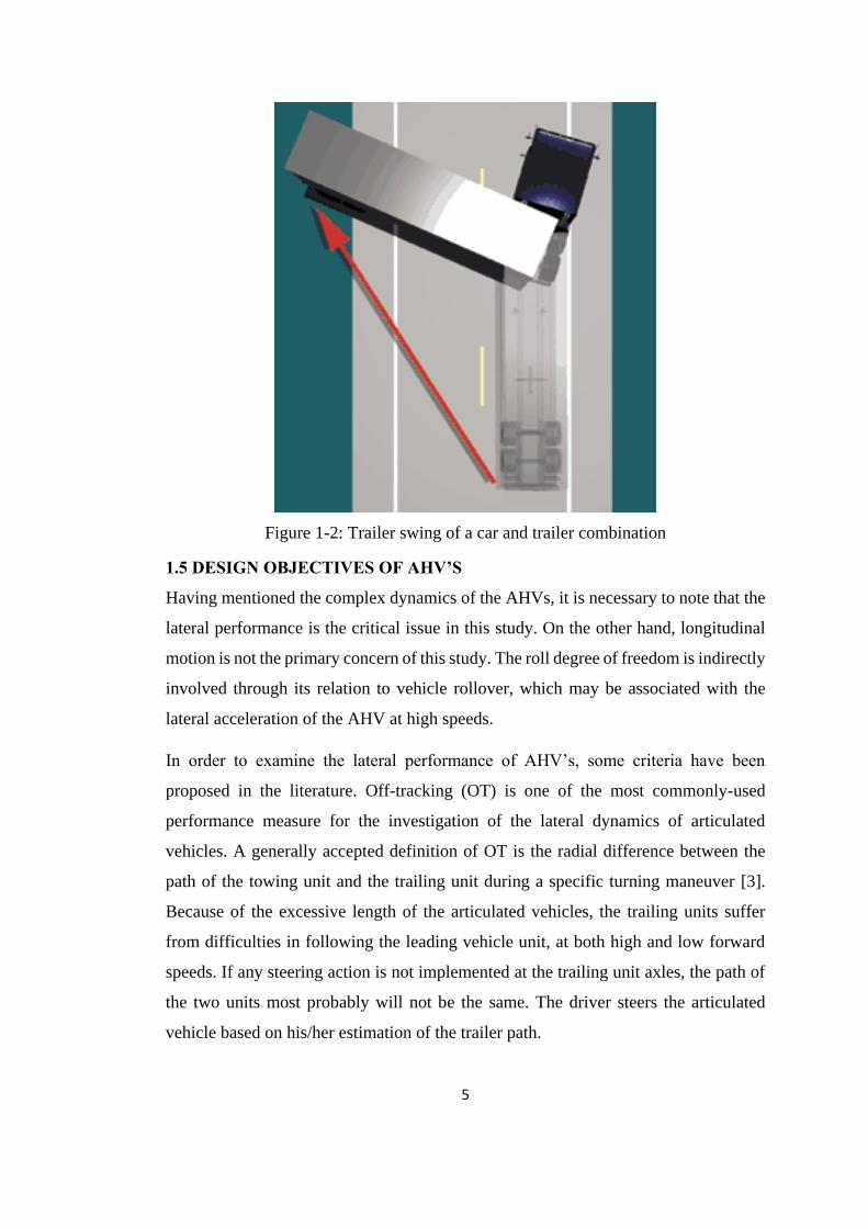
Second unstable motion mode of the articulated vehicles is called as trailer swing. As
it is reflected in its name, uncontrolled lateral motion of the trailing unit take place in
that case. Large motion of the trailing unit usually leads to sweeping of the other
vehicles next to the AHV. Both unstable modes mentioned here may result from
sudden excessive steering angles at high speeds as well as locked wheels of the rear
axles of the tractor or trailer due to excessive braking. Figure 1-2 is an illustration of
trailer swing case experienced by a car and trailer combination.
Rollover is the third type of the unstable motion modes of the AHVs. The most likely
cause of rollover is high lateral acceleration of the trailing units. During the lane
change maneuvers at high forward speeds, lateral acceleration of the trailing units is
usually higher than that of the towing unit. Therefore, high roll angles of the trailing
unit may result in the rollover of the vehicle. Center of gravity (COG) height, vehicle
speed, steering actions etc. are the major factors that have influence on the rollover of
the vehicle.
5
Figure 1-2: Trailer swing of a car and trailer combination
1.5 DESIGN OBJECTIVES OF AHV’S
Having mentioned the complex dynamics of the AHVs, it is necessary to note that the
lateral performance is the critical issue in this study. On the other hand, longitudinal
motion is not the primary concern of this study. The roll degree of freedom is indirectly
involved through its relation to vehicle rollover, which may be associated with the
lateral acceleration of the AHV at high speeds.
In order to examine the lateral performance of AHV’s, some criteria have been
proposed in the literature. Off-tracking (OT) is one of the most commonly-used
performance measure for the investigation of the lateral dynamics of articulated
vehicles. A generally accepted definition of OT is the radial difference between the
path of the towing unit and the trailing unit during a specific turning maneuver [3].
Because of the excessive length of the articulated vehicles, the trailing units suffer
from difficulties in following the leading vehicle unit, at both high and low forward
speeds. If any steering action is not implemented at the trailing unit axles, the path of
the two units most probably will not be the same. The driver steers the articulated
vehicle based on his/her estimation of the trailer path.
6
Rearward amplification ratio (RWA) is another term frequently used in the literature
as a performance measure of articulated heavy vehicles. The definition of the term is
expressed as the peak lateral acceleration ratio of the trailing unit to that of the towing
unit for an articulated vehicle [4]. The reason why RWA ratio has been a widely-used
performance criterion is its utility in the roll study. As a rule of thumb, the lower RWA
ratio implies the higher lateral stability of the articulated vehicle. That is, minimization
of RWA ratio will serve the purpose of reducing the probability of rollover.
1.6 THESIS ORGANIZATION
In this introductory chapter, a brief overview of the types and characteristics of
articulated heavy vehicles relevant to the basic subject of the thesis study is provided.
Lateral dynamics and typical instabilities of AHVs are identified. Then, the
explanation of major design objectives is given.
The second chapter mainly focuses on the review of the literature on trailer steering
systems of the articulated heavy vehicles. In order to construct a background in the
topic, relevant vehicle models and their verification methods are stated. Moreover,
various trailer steering strategies found in the literature are examined.
The third chapter moves on to describe the dynamic model of the tractor and multi-
axle semi-trailer. The derivation of the suggested dynamic model is explained and
discussed in sufficient detail.
The fourth chapter introduces the active trailer steering (ATS) control strategies
including both some classical and relatively more recent approaches in the literature,
and the strategy proposed in this study. For each control strategy, the fundamental idea
behind the methods is explained together with the derivation of the controller designs.
Chapter 5 includes the simulation results obtained for each of the controllers
introduced in the previous chapter. The lateral performance of the tractor and semi-
trailer combination is investigated at both low and high speed travel conditions.
The last chapter provides a brief summary of the comparative performance evaluation
of the existing and the proposed ATS control strategies at low and high forward speeds.

7
CHAPTER 2
LITERATURE REVIEW
The rapid growth in the use of heavy commercial vehicles brings about the necessity
of improved design of the AHV’s. Thus, the topic of trailer steering in articulated
heavy vehicles has been and still is an active research area of vehicle dynamics. Over
the past years, a considerable amount of literature has been published on trailer steering
systems of AHV’s. It has become commonplace to distinguish the passive and active
types of trailer steering systems. Although previous studies have primarily
concentrated on passive trailer steering (PTS) systems, new developments give rise to
studies that focus on the active steering systems for trailers.
Before proceeding to examine various kinds of trailer steering strategies, the vehicle
models used in the previous studies, lateral performance measures and corresponding
standard maneuvers will be presented.
2.1 ARTICULATED HEAVY VEHICLE MODELS
For a successful application of trailer steering, the proper modeling of articulated
vehicle is required. Several studies investigating the trailer steering systems have made
use of different vehicle models. The most frequently used vehicle models in the study
of lateral performance of AHV’s are linear yaw plane models[5][6][7][8][9][10]. As
far as the lateral characteristics of the articulated vehicles concerned, the sufficiency
of linear yaw plane models has been proved in the literature. The validation of linear
yaw plane models of AHV’s have been verified by the comparison with some
advanced commercial software. Changfu et al. [11] performed the verification of a 6-
axle linear articulated vehicle model in case of drastic handling situations. According

8
to their research, the responses obtained by the proposed linear yaw plane model has
a decent agreement with those obtained by using TruckSim® software for the case of
an extreme handling maneuver. Furthermore, higher order non-linear planar models
are also investigated. Azadi et al. [12] suggested a higher order yaw plane model
integrated with a nonlinear tire model.
In the recent studies, on the other hand, the additional degrees of freedom have been
considered in the vehicle dynamics models. Especially, the researches including the
roll dynamic of the vehicles require advanced models to be used [13]. Cebon et al. [14]
used linear vehicle model comprising the roll degree of freedom in their study.
Likewise, Islam utilized a similar roll/yaw vehicle model and performed its validation
via TruckSim® reference model [15]. Further, a nonlinear roll/yaw vehicle model was
used by Azadi, who verified the vehicle model via real test data [16].
To conclude with, researchers have examined several vehicle dynamic models for
simulations and controller design. Review of the above literature shows that up to date
studies focus on more improved models of AHVs. However, linear yaw/plane models
are still quite popular due to their advantageous features of suitability for controller
design and sufficient accuracy for simulation purposes.
2.2 PERFORMANCE MEASURES
For the assessment of lateral performance of articulated vehicles controlled with trailer
steering strategies, various criteria have been developed. Commonly-used
performance measures found in the literature for the AHV’s lateral motion are listed
in Table 2-1 together with their explanations.
As understood by the explanations on the Table 2-1, the performance measures are
taken during standardized test maneuvers of AHVs. The specified standard test
conditions mentioned in the explanation of the performance measures are provided in
next section.

9
Table 2-1: Commonly used performance measures adapted from [17]
PERFORMANCE
MEASURE EXPLANATION
Low Speed Swept Path Width
(SPW)
Maximum lateral offset between the paths of
COG’s of tractor & semi-trailer units during
specific constant radius turning maneuver
Static Rollover Threshold Maximum lateral acceleration just before the
rollover of the articulated vehicle
Low-speed Off-tracking
(LSOT)
Maximum width of the path swept by the
AHV during specific 90-degree intersection
turn
Yaw Damping Coefficient Minimum damping ratio at the articulation
joints of the vehicle during free oscillations
Rearward Amplification
(RWA)
The ratio of the peak lateral acceleration at
trailer COG to that of towing unit at specific
high speed lane change maneuver
High-speed Transient Off-
tracking (TOT)
Maximum lateral distance between the path
of tractor front axle center and semi-trailer
rear axle center during specific lane change
maneuver
High-speed Steady State Off-
tracking (HSOT)
Maximum lateral distance between the path
of tractor front axle center and semi-trailer
rear axle center during specific high speed
steady state turning maneuver
Load Transfer Ratio The ratio of the total lateral forces on either
side of the articulated heavy vehicle
Steer Tire Friction Demand The ratio of normalized horizontal force to
the available peak friction
Tail Swing Maximum lateral offset the rear corner of the
vehicle travel outside of the front wheel path
As mentioned in the previous section, the most frequently used performance measures
are RWA and PFOT (known as LSOT/HSOT at low/high speed conditions). In order
to better understand these criteria, typical illustrations are presented in Figure 2-1 and
Figure 2-2.

10
RWA is based on the peak values of lateral acceleration responses of the towing and
trailing units. In Figure 2-1, 𝑃𝑟 and 𝑃𝑓 represent the peak values of lateral accelerations
of trailer and tractor units. RWA value is calculated by taking the ratio of 𝑃𝑟 to 𝑃𝑓.
Figure 2-1: Illustration of rearward amplification ratio (RWA) [9]
PFOT is described as the maximum swept width between the paths followed by the
tractor and semi-trailer units. In Figure 2-2, largest distance between the solid line and
the dashed line identifies the PFOT measure.
Figure 2-2: Illustration of path-following off-tracking (PFOT) [9]

11
2.3 STANDARD MANEUVERS
After reviewing general lateral performance measures for the AHV’s, it is necessary
to specify the standard maneuvers on which these measures are taken. Researchers
have tried different maneuvers for both low and high speed cases, some of which have
been standardized internationally. Below are some examples to commonly used
standard maneuvers.
In the research conducted by Fancher and Winkler [4], the authors investigated the
single lane change maneuver identified previously by International Standards
Organization (ISO) in 2000. According to the study, the single sine-wave lateral
acceleration input had been described as follows: A minimum lateral acceleration of
0.15g must be achieved at the front axle of the towing unit. The required steering input
must be in the period of 0.4 Hz which can be converted to 2.5 seconds. The longitudinal
speed of the vehicle combination should be 88 km/h. Similarly, SAE J2179 testing
maneuver describes a single lane change at 88 km/h, allowing 1.464 m lateral offset
for 61 m longitudinal distance [14]. In general, these maneuvers have been used for
the evaluation of rearward amplification (RWA) ratio and transient state off-tracking
(TOT) obtained by the relevant vehicle dynamic simulations.
High speed constant radius turning maneuver is described as traveling of the AHV at
the speed of 100 km/h while the front axle centerline of the towing unit follows the
path of a 393 m radius circle [17]. With this maneuver, the high-speed steady state off-
tracking (HSOT) values can be obtained.
According to the study conducted by Jujnovich and Cebon [18], low speed circle
turning maneuver and low speed 90° intersection turn maneuver are defined at a
vehicle forward speed of 10 km/h. The towing unit of the AHV must follow the path
of 11.25 m circle during both turning maneuvers. The lateral performance measure,
low speed swept path, is obtained by using low speed circle turning maneuver. Also,
low speed off-tracking (LSOT) is measured by implementing low speed 90°
intersection turn maneuver.

12
2.4 PASSIVE TRAILER STEERING SYSTEMS
The lateral performance of the AHV’s has been improved with the implementation of
trailer steering systems. In order to resolve the lateral performance issue, a reasonable
approach was introduced with the utilization of the passive trailer steering (PTS)
systems. Several types of PTS systems have been proposed in the literature, consisting
of self-steering, command steering, and pivotal bogie systems. As implied by its name,
PTS systems apply the steering action to the corresponding trailer axles in a passive
manner. For some PTS systems like self-steering, the forces created by the tire-road
interactions determine the steering angle of the trailer wheels. However, the
determination of trailer steering angle in PTS systems is generally done based on the
value of the articulation angle between the vehicle units. Command steering and
pivotal bogie systems make use of the rule mentioned above, i.e. the wheels of the
trailer are steered at an angle proportional to the hitch angle.
2.4.1 Self-steering Systems
The first classic example of the passive trailer steering system is self-steering.
According to LeBlanc et al. [19], self-steering systems were first developed to be used
as a second axle of a tandem axle group on straight trucks. The major aim was to
reduce off-tracking and tire scuffing in tight turns. The influences of self-steering axles
on the steady-state handling performance of some AHV configurations are discussed
in their research. A similar research conducted by Nisonger and Macadam has
demonstrated that self-steering axles increase low-speed maneuverability as well as
reducing the tire wear [20]. In another study, Luo examined the directional
characteristics and performance of self-steered axles together with the liftable axles
[21]. The results of his work reveal that self-steering axles possess large friction
demand at both low and high speeds, suggesting high risk of jack-knifing.
2.4.2 Command-steering Systems
Command steering is another well-known example of PTS systems. For passive
command steering systems, the rearmost trailer wheels are steered by an angle in
relation to the articulation angle between the units via a mechanism. Figure 2-3
illustrates an example of a command steering mechanism.

13
Figure 2-3: Command steering mechanism[2]
In 1991, Sankar et al. [22] published a paper in which they compared the lateral
performance in cases of using command steering and self-steering systems. In their
study, command steering is identified as forced steering, where the steering angle is
expressed as a function of the articulation angle and the front wheel steering angle. In
a more recent work, Özkan et al. [23] reported a study related to the minimization of
tire wear with command-steering. An optimization procedure is used in their
investigation to achieve a reduction of tire wear on AHV’s without deteriorating the
vehicle path. Both studies demonstrated that command trailer steering systems
enhances the low-speed lateral performance of the articulated vehicles. The above
finding is also consistent with the study carried out by Jujnovich and Cebon [18]. To
conclude, the results of the studies reveal that low-speed maneuverability of the
vehicle is improved as a consequence of the command steering.
2.4.3 Pivotal Bogie Steering Systems
Similar to command trailer steering, pivotal bogie systems utilize the trailer steering
action depending on the articulation angle of the AHV. Pivotal bogie system differs
from command steering in one main principle. In this PTS system, the whole bogie set
is steered instead of individual axles of the trailer, causing additional complexity to
the trailer steering system. An illustration of a pivotal bogie mechanism is given in
Figure 2-4. Several bogie steering mechanisms have been patented in the past decade
[24][25][26]. However, the implementation of modern bogie mechanism for the PTS
systems has been introduced recently. Being a new type of pivotal bogie steering

14
system, Trackaxle® PTS system earned popularity in 2000’s [27]. In the paper, Prem
et al. indicated that the Trackaxle® PTS system offers enhanced safety and efficiency
as well as reduced harm to the roads. In a different study[28], Prem and Atley
mentioned potential benefits of the PTS system in many areas. They claimed that the
Trackaxle® pivotal bogie system offers superior low speed off-tracking ability as well
as reductions in road damage and tire scuffing. Furthermore, Jujnovich and Cebon [29]
performed an experimental investigation on an articulated test vehicle in which its
trailer is supported with pivotal bogie steering strategy. The outcome of their work was
consistent with the results of the previous studies.
Figure 2-4: Pivotal bogie mechanism
2.5 ACTIVE TRAILER STEERING SYSTEMS
The primary goal of recent trailer steering researches is the development of a method,
which can provide acceptable performance for a wide range of longitudinal vehicle
speeds. Since all the previously stated PTS methods suffer from some serious
limitations at high speeds, recent developments have emphasized the need for active
trailer steering (ATS) strategies. Thus, recently, ATS systems have been one of the
major research subjects on the articulated vehicle studies.
In order to accomplish the contradictory design objectives of AHVs at both low and
high speeds, various active steering strategies have been proposed in the literature

15
[30][31][32]. These strategies can be classified under five categories as steer ratio
principle, active command steering, reference model tracking, path-following and
time-lag types. Following subsections identify the classified types of the control
strategies found in the literature.
2.5.1 Steer Ratio Principle
In the past studies, steer ratio was a commonly-used trailer steering principle in
articulated vehicles. In the literature, the term refers to the steering action on the towing
units proportional to the steer angle of tractor unit or directional velocity. In the
analysis of Wu and Lin, the influence of additional steerable trailer axles on the
dynamic lateral performance was examined [33]. The control method suggested the
steering of the trailer axle wheels in relation to the front steering angle of the tractor
unit, concerning the forward vehicle speed. The corresponding steer ratio was
determined by making the side slip angle equal to zero in steady state turning situations
at all forward speeds. Three important conclusions of their study was the enhancement
in lateral stability, reduction in phase delay of trailer unit, and improvement in
maneuverability of vehicle. Furthermore, Wu [34] obtained similar findings in his next
study, concerning the effect of roll degree of freedom in the investigation. In a more
recent work, Rangavajhula and Tsao compared the off-tracking performance of AHV
by implementing trailer steering at particular steer ratios [35]. The researchers have
confirmed that trailer steering led to less off-tracking at all forward speeds. On the
other hand, the researchers have observed the major weakness of steer ratio approach
at high speeds.
2.5.2 Active Command Steering Strategy
Rangavajhula and Tsao proposed an active steering strategy mainly established with
regard to a previously mentioned PTS method [5]. The trailer steering strategy was
implemented on an AHV combination involving a number of trailers. The
investigation of the command steering based active optimal control has utilized the
geometric relation with the articulation angle, similar to the passive system. According
to the study, the passive command steering is very effective in reducing off-tracking

16
only at low speeds, whereas the active one provides superior lateral performance at
low to medium speeds.
2.5.3 Reference Model Tracking Strategy
Another strategy in active trailer steering systems can be identified as reference model
tracking. Oreh et al. [32] have suggested an ATS strategy that tries to follow ideal
reference responses of side slip, yaw rate, and articulation angle. Actually, they defined
a desired set of vehicle states that the trailer should track. According to the study, the
tracking of ideal side slip velocity and yaw rate characteristics is very effective in the
lateral performance of the AHV only at high speed conditions. In contrast, this result
in practically no improvement at low speeds. Furthermore, following the trajectory of
proposed reference articulation angle exhibits good off-tracking performance at both
low and high vehicle speeds. Another study conducted by Oreh, Kazemi and Azadi
have suggested an ATS strategy, tracking a desired articulation angle between the units
[12]. The authors have stated that the following of reference articulation angle provides
a more direct method compared to the other techniques in terms of path-following. The
reference hitch angle of the proposed method is calculated regarding the rear end of
the semi-trailer to follow the fifth wheel path. A fuzzy logic controller (FLC) is
implemented in the research to track the ideal trajectory of the hitch angle. As a
conclusion, the lateral performance of the proposed method is effective in terms of off-
tracking. In their next study [16], the authors have obtained similar findings by
investigating another reference model tracking controller.
2.5.4 Path-following Type Strategies
Path-following ATS strategies are one of the most commonly used type in articulated
vehicles. A considerable amount of literature has been published on that strategy up to
now. In 1991, Notsu et al. [36] introduced an ATS strategy, called as path-following
control method. The aim of the study was to suppress the swaying oscillations of
trailers as well as providing better off-tracking performance. The basic idea behind the
strategy was the steering of trailer axle wheels so that the rear end of the trailing unit
should follow the front end of the towing unit. In the study, the required trailer steering
angles are determined after the estimation of tractor path with the use of a
17
mathematical model. According to the research, the low speed off-tracking ability of
the articulated test vehicle has improved with the utilization of the control method.
However, there has been some discussion about the limitations and drawbacks of the
study. After the introduction of the path-following strategy, many scientists pursue the
development of Notsu’s idea. In a recent work, Jujnovich and Cebon [37] have
analyzed the CT-AT path following strategy, meaning an active trailer (AT) unit
tracking its conventional tractor (CT) unit. The strategy has focused on the idea that
the centerline of trailer rear end (follow point) should correctly track the articulation
point (lead point). Detailed analyses at high speed cases are performed. However, the
drawbacks of the method at low speed cases appeared. Furthermore, the researchers
have concluded that the proposed strategy cannot make the fifth wheel to follow the
front of the tractor unit. To preclude the situation, they have utilized an AT-AT strategy
applying an additional steering action on the drive axles of the tractor unit. According
to their conclusion, AT-AT strategy performed slightly better than the CT-AT strategy
due to the extra steering action on tractor axles. In a similar study, Roebuck et al. [38]
have designed a path-following controller for an AHV in case of high speed
maneuvers. An AHV consisting of a truck, a dolly and a semi-trailer are first modeled
for the implementation of the LQR controller. Afterwards, a Kalman filter is used to
estimate all the vehicle states and the positions of the follow and lead points. The main
objective of the optimal controller was to minimize the errors between the path of
follow points and lead points of relevant vehicle units. In other words, the dolly tries
to follow the path of the truck whereas the semi-trailer aims to follow the dolly path.
Further investigation is performed via the implementation of the controller on a test
vehicle, where the trailer axles are steered by hydraulic actuators. The results of the
study have verified that the suggested path-following controller reduced the off-
tracking and RWA of the vehicle. Different from the past studies, the research
conducted by Cheng et al. [14] have examined a path-following controller in
combination with a roll stability controller. The authors utilized optimal control
methods, enhancing roll stability without deteriorating the path tracking ability. The
relevant cost function of the LQR has regarded the path following error and RWA ratio
as parameters to be minimized. The results demonstrated that the roll stability is

18
improved while keeping the path-following errors in an allowable ranges. Islam and
He [3] proposed the lateral position deviation preview (LPDP) controller to prevent
the unstable modes of the AHV’s. The suggested model can also be considered as a
path-following controller, offering a simpler way of path-tracking by appropriate
matrix manipulations. All the papers published recently about the path-following
controllers verifies the convenience of the approach in the field of active articulated
trailer steering [39][40][41].
As distinct from other studies, Ding, Mikaric, and He tested the performance of an
ATS system applying the optimal control in real time simulations [42]. A simulation
environment is constructed consisting of a vehicle model on TruckSim®, an optimal
controller, and the driver. In order to determine the active steering angles of the trailer
wheels, a linear quadratic regulator (LQR) working in real time is used as ATS
controller. The authors point out that the study has demonstrated the enhancement in
low speed maneuverability. Also, improvement on high speed stability of the
articulated vehicle is stated.
In his study, Islam has proposed a new approach called as two design loop (TDL) and
single design loop (SDL) method [31]. In the study, the aim was to implement an active
trailer steering system together with the design optimization of passive trailer
variables. In order to better explain the approach, the main principle of TDL and SDL
method is identified as follows: Optimal controller parameters are found for low speed
and high speed cases, using Genetic Algorithm technique. Besides, the passive design
variables of trailing unit such as the mass, inertia and distances between the trailer
axles are determined in their allowable ranges. Both methods utilize the same principle
with one significant difference. The TDL method computes the passive trailer
variables after the controller design, whereas SDL performs the calculations in a single
loop simultaneously. In his next study, Islam et al. [43] have concluded that the
methods improve low speed maneuverability and high speed lateral stability.
2.5.5 Time-lag Strategy
Kharrazi et al. [44] proposed a different active trailer steering strategy. The approach
was based on the regulation of the time delay between the steering action of the driver

19
and the creation of lateral forces on the trailing axle wheels. For any kind of vehicle,
the lateral tire forces are developed as a reaction to the driver steering input. However,
the formation of the tire forces on trailing units require some time after the instant the
driver steers the towing vehicle unit. The steering-based controller aims to regulate the
timing of active steering of the trailer wheels so that the formation of trailer tire forces
would be compatible with the steering action of the driver. The performance of the
proposed controller has been tested with the use of computer simulations as well as
the implementation on a test vehicle. A significant reduction in RWA ratio and off-
tracking, without deteriorating the maneuverability, has been observed. In their next
study, Kharrazi, Lidberg and Fredriksson have applied the same ATS strategy, named
as the generic controller at that time [45]. Implementing the time-delay controller
approach, several different combinations of articulated heavy vehicles have been
compared in terms of various lateral performance measures. As a result of the study,
the suggested controller has been verified as effective for all vehicle combinations.
The details of the both articles could be seen in the dissertation of Kharrazi [9].
2.6 MOTIVATION AND SCOPE OF THE STUDY
Regarding the significance of AHV’s in transport technology, the proper design of
articulated heavy vehicles is of great importance, particularly with respect to safety.
The present study focuses on the modeling and active steering control of articulated
vehicles with multi-axle semi-trailers. The improvement of the lateral performance of
tractor semi-trailer combinations for both low and high speeds is the major focus of
the study.
The fundamental design objectives for articulated heavy vehicles have been PFOT and
RWA, at low and high vehicle longitudinal speeds, respectively. The high speed lateral
performance of an AHV, as indicated by the design objectives, deteriorates while
meeting the low speed design goals and vice versa [4]. Therefore, a successful method
should be developed to meet both high and low speed requirements at the same time.
The main subject of the study is to resolve the conflicting design objectives at different
vehicle speeds by developing a strategy for the active steering of the semitrailer axles.

20

21
CHAPTER 3
MODELING
Having discussed the literature in the previous chapter, the purpose of this chapter is
to provide a detailed explanation of modeling of the tractor and multi-axle semi-trailer
combination. The derivation procedure of the 5 degree of freedom (DOF) yaw/roll
vehicle model is expressed in detail.
First of all, the complete description of the AHV is provided. The modeled tractor
comprises a steerable axle at the front and drive tandem axles at the back. The trailing
unit is connected with the tractor unit by means of a fifth wheel located at the
articulation point. The semi-trailer has three axles at the back side that are
conventionally unsteered. In the Figure 3-1, however, all the semi-trailer axles are
shown with steering angles in order to represent the forces created in case of active
steering of each axle tires.
In the yaw/roll model demonstrated in Figure 3-1 and Figure 3-2, ISO reference
coordinate system is used, meaning that the orientation of the X,Y and Z axes indicate
the forward, upward and left side of the vehicle, respectively. In order to simplify the
appearance of the model, each axle is represented by one equivalent wheel in the
figure. The equations of motions are derived with the use of Newton’s laws of
dynamics.
The 5 DOFs of the yaw/roll vehicle model are expressed with the following terms: the
side slip of the tractor 𝑣, the yaw rate of the tractor 𝑟, the roll angle of the tractor 𝜙,
the yaw rate of the semi-trailer 𝑟𝑡, and roll angle of semi-trailer 𝜙𝑡. Note that the side

22
slip of semi-trailer is a depended term that can be represented as a combination of other
states. For better understanding the terms denoted in the vehicle model, a brief look at
the nomenclature (provided at the beginning of the thesis) may be necessary.
The basic assumptions in the derivation of the articulated vehicle model could be listed
as follows:
Body centered coordinate systems are fixed to the center of gravities (COG) of
towing and trailing vehicle units.
The total masses of the tractor and semi-trailer are lumped at their COGs as
point masses.
The stiffness of the tires is combined so that the equivalent cornering stiffness
is the total stiffness of the wheels on the same axle.
The lateral tire forces are assumed as a linear function of tire slip angles.
Longitudinal tire forces such as traction and braking forces are ignored due to
their relatively small influence on lateral dynamics of the AHV. That is, the
tire forces on the x-directions are neglected.
Pitch and bounce motion of both AHV units are irrelevant to the thesis topic
and ignored.
The velocities at the articulation point of towing and trailing units are
compatible since both units are considered to travel at a constant forward speed
U.

23
Figure 3-1: Bicycle model of the tractor and semi-trailer combination
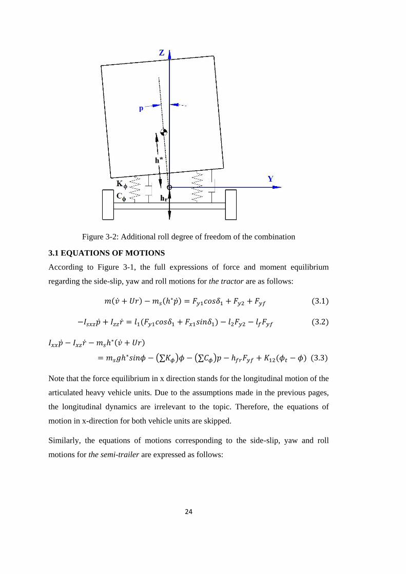
24
Figure 3-2: Additional roll degree of freedom of the combination
3.1 EQUATIONS OF MOTIONS
According to Figure 3-1, the full expressions of force and moment equilibrium
regarding the side-slip, yaw and roll motions for the tractor are as follows:
𝑚(�̇� + 𝑈𝑟) − 𝑚𝑠(ℎ∗�̇�) = 𝐹𝑦1𝑐𝑜𝑠𝛿1 + 𝐹𝑦2 + 𝐹𝑦𝑓 (3.1)
−𝐼𝑠𝑥𝑧�̇� + 𝐼𝑧𝑧�̇� = 𝑙1(𝐹𝑦1𝑐𝑜𝑠𝛿1 + 𝐹𝑥1𝑠𝑖𝑛𝛿1) − 𝑙2𝐹𝑦2 − 𝑙𝑓𝐹𝑦𝑓 (3.2)
𝐼𝑥𝑥�̇� − 𝐼𝑥𝑧�̇� − 𝑚𝑠ℎ∗(�̇� + 𝑈𝑟)
= 𝑚𝑠𝑔ℎ∗𝑠𝑖𝑛𝜙 − (∑𝐾𝜙)𝜙 − (∑𝐶𝜙)𝑝 − ℎ𝑓𝑟𝐹𝑦𝑓 + 𝐾12(𝜙𝑡 − 𝜙) (3.3)
Note that the force equilibrium in x direction stands for the longitudinal motion of the
articulated heavy vehicle units. Due to the assumptions made in the previous pages,
the longitudinal dynamics are irrelevant to the topic. Therefore, the equations of
motion in x-direction for both vehicle units are skipped.
Similarly, the equations of motions corresponding to the side-slip, yaw and roll
motions for the semi-trailer are expressed as follows:

25
𝑚𝑡(�̇�𝑡 + 𝑈𝑡𝑟𝑡) − 𝑚𝑠𝑡(ℎ𝑡∗𝑝�̇�)
= −𝐹𝑦𝑓𝑐𝑜𝑠𝛹 + 𝐹𝑦3𝑐𝑜𝑠𝛿3 + 𝐹𝑦4𝑐𝑜𝑠𝛿4 + 𝐹𝑦5𝑐𝑜𝑠𝛿5 (3.4)
−𝐼𝑠𝑥𝑧𝑡𝑝�̇� + 𝐼𝑧𝑧𝑡�̇�𝑡
= −𝑙3𝐹𝑦3𝑐𝑜𝑠𝛿3 − 𝑙4𝐹𝑦4𝑐𝑜𝑠𝛿4 − l5𝐹𝑦5𝑐𝑜𝑠𝛿5
− 𝑙𝑓𝑡𝐹𝑦𝑓cos𝛹 (3.5)
𝐼𝑥𝑥𝑡𝑝�̇� − 𝐼𝑥𝑧𝑡𝑟�̇� −𝑚𝑠𝑡ℎ𝑡∗(𝑣�̇� + 𝑈𝑡𝑟𝑡)
= 𝑚𝑠𝑡𝑔ℎ𝑡∗𝑠𝑖𝑛𝜙𝑡 − (∑𝐾𝜙𝑡)𝜙𝑡 − (∑𝐶𝜙𝑡)p𝑡 + ℎ𝑓𝑟𝑡𝐹𝑦𝑓cos𝛹
− 𝐾12(ϕ𝑡 − ϕ) (3.6)
In addition to the previous expressions, the compatibility equation for the velocities on
the fifth wheel is expressed as follows:
𝑈𝑡 = 𝑈𝑐𝑜𝑠𝛹 − 𝑣𝑠𝑖𝑛𝛹 + 𝑙𝑓𝑟𝑠𝑖𝑛𝛹 (3.7)
𝑣𝑡 = 𝑈𝑠𝑖𝑛𝛹 + 𝑣𝑐𝑜𝑠𝛹 − 𝑙𝑓𝑟𝑐𝑜𝑠𝛹 − 𝑙𝑓𝑡𝑟𝑡 − ℎ𝑓𝑟𝑝 + ℎ𝑓𝑟𝑡𝑝𝑡 (3.8)
Note that the tire lateral forces 𝐹𝑦𝑖’s are assumed as a function of cornering stiffness
and slip angles as indicated in Equation (3.9).
𝐹𝑦𝑖 = ∑𝐶𝑠𝑖𝛼𝑖 = 𝐶𝑖𝛼𝑖 𝑓𝑜𝑟 𝑖 = 1,2,3,4,5 (3.9)
Furthermore, the non-linear expressions of the slip angles 𝛼𝑖 for ith axle wheels are
written in the following equations.
𝛼1 = tan−1 (
𝑣 + 𝑙1𝑟
𝑈) − 𝛿1 (3.10)
𝛼2 = tan−1 (
𝑣 − 𝑙2𝑟
𝑈) (3.11)
𝛼3 = tan−1 (
𝑣𝑡 − 𝑙3𝑟𝑡𝑈𝑡
) + 𝛿3 (3.12)
𝛼4 = tan−1 (
𝑣𝑡 − 𝑙4𝑟𝑡𝑈𝑡
) + 𝛿4 (3.13)
𝛼5 = tan−1 (
𝑣𝑡 − 𝑙5𝑟𝑡𝑈𝑡
) + 𝛿5 (3.14)

26
Manipulating the equations from (3.1) to (3.14), the final linearized version of the
differential equations is obtained (see Appendix A for details) as follows:
{𝑚}�̇� + {𝑚𝑡}𝑣�̇� + {−𝑚𝑠ℎ∗}�̇� + {−𝑚𝑠𝑡ℎ𝑡
∗}𝑝�̇�
= {𝐶1 + 𝐶2𝑈
} 𝑣 + {𝐶3 + 𝐶4 + 𝐶5
𝑈} 𝑣𝑡 + {
𝐶1𝑙1 − 𝐶2𝑙2 −𝑚𝑈2
𝑈} 𝑟
+ {−𝐶3𝑙3 − 𝐶4𝑙4 − 𝐶5𝑙5 −𝑚𝑡𝑈
2
𝑈} 𝑟𝑡 + {−𝐶1}𝛿1 + {𝐶3}𝛿3 + {𝐶4}𝛿4
+ {𝐶5}𝛿5 (3.15)
{𝑚𝑙𝑓}�̇� + {𝐼𝑧𝑧}�̇� + {−𝐼𝑠𝑥𝑧 −𝑚𝑠ℎ∗𝑙𝑓}�̇�
= {𝐶1𝑙1 − 𝐶2𝑙2 + (𝐶1 + 𝐶2)𝑙𝑓
𝑈}𝑣
+ {𝐶1𝑙1
2 + 𝐶2𝑙22 + (𝐶1𝑙1 − 𝐶2𝑙2 −𝑚𝑈
2)𝑙𝑓𝑈
} 𝑟
+ {−𝐶1(l1 + 𝑙𝑓)}𝛿1 (3.16)
{𝑚ℎ𝑓𝑟 −𝑚𝑠ℎ∗}�̇� + {−𝐼𝑠𝑥𝑧}�̇� + {𝐼𝑠𝑥𝑥 −𝑚𝑠ℎ
∗ℎ𝑓𝑟}�̇�
= {(𝐶1 + 𝐶2)ℎ𝑓𝑟
𝑈}𝑣 + {
(𝐶1𝑙1 − 𝐶2𝑙2 −𝑚𝑈2)ℎ𝑓𝑟 + 𝑚𝑠𝑈
2ℎ∗
𝑈} 𝑟
+ {−∑𝐶𝜙}𝑝 + 𝑚𝑠ℎ∗𝑔 − ∑𝐾𝜙 − 𝐾12𝜙 + {𝐾12}ϕ𝑡
+ {−𝐶1ℎ𝑓𝑟}𝛿1 (3.17)
{−𝑚𝑡𝑙𝑓𝑡}𝑣�̇� + {𝐼𝑧𝑧𝑡}�̇�𝑡 + {𝐼𝑠𝑥𝑧𝑡 +𝑚𝑠𝑡ℎ𝑡∗𝑙𝑓𝑡}𝑝�̇�
= {−𝐶3(𝑙3 + 𝑙𝑓𝑡) − 𝐶4(𝑙4 + 𝑙𝑓𝑡) − 𝐶5(𝑙5 + 𝑙𝑓𝑡)
𝑈} 𝑣𝑡
+ {𝐶3𝑙3
2 + 𝐶4𝑙42 + 𝐶5𝑙5
2 + (𝐶3𝑙3 + 𝐶4𝑙4 + 𝐶5𝑙5 +𝑚𝑡𝑈2)𝑙𝑓𝑡
𝑈} 𝑟𝑡
+ {−𝐶3(𝑙3 + 𝑙𝑓𝑡)}𝛿3 + {−𝐶4(𝑙4 + 𝑙𝑓𝑡)}𝛿4
+ {−𝐶5(𝑙5 + 𝑙𝑓𝑡)}𝛿5 (3.18)
27
{𝑚𝑡ℎ𝑓𝑟𝑡 −𝑚𝑠𝑡ℎ𝑡∗}𝑣�̇� + {−𝐼𝑠𝑥𝑧𝑡}𝑟�̇� + {𝐼𝑠𝑥𝑥𝑡 −𝑚𝑠𝑡ℎ𝑡
∗ℎ𝑓𝑟𝑡}𝑝�̇�
= {(𝐶3 + 𝐶4 + 𝐶5)ℎ𝑓𝑟𝑡
𝑈}𝑣𝑡
+ {−ℎ𝑓𝑟𝑡(𝐶3𝑙3 + 𝐶4𝑙4 + 𝐶5𝑙5 +𝑚𝑡𝑈
2) + 𝑚𝑠𝑡𝑈2ℎ𝑡
∗
𝑈} 𝑟𝑡
+ {−∑𝐶𝜙𝑡}p𝑡 + {𝐾12}ϕ + {𝑚𝑠𝑡ℎ𝑡∗𝑔 − ∑𝐾𝜙𝑡 − 𝐾12}𝜙𝑡 + {𝐶3ℎ𝑓𝑟𝑡}𝛿3
+ {𝐶4ℎ𝑓𝑟𝑡}𝛿4 + {𝐶5ℎ𝑓𝑟𝑡}𝛿5 (3.19)
{−1}�̇� + {1}�̇�𝑡 + {𝑙𝑓}�̇� + {𝑙𝑓𝑡}�̇�𝑡 + {−ℎ𝑓𝑟}�̇� + {ℎ𝑓𝑟𝑡}𝑝�̇� = {𝑈}𝑟 + {−𝑈}𝑟𝑡 (3.20)
{1}�̇� = {1}𝑝 (3.21)
{1}𝜙𝑡̇ = {1}𝑝𝑡 (3.22)
These differential equations provide the base for the state space system modeling in
the next section.
3.2 STATE-SPACE SYSTEM MODELING
Before proceeding to examine the construction of state-space matrices, it is crucial to
address the theory behind the method. In control engineering, a state space system may
be defined as a mathematical model of a physical system. The approach is said as a
generalized time domain technique for modelling, analyzing and designing a wide
range of control systems. A significant characteristics of state space modeling is its
superior suitability with digital computational methods. The modeling in state space is
preferred due to its ease of use on the software employed in this study, MATLAB®.
In order to construct a state-space representation, the equations of motions should be
expressed as a set of first-order differential equations in terms of the state and the input
variables. If the original dynamic system is identified as linear time invariant
equations, the application of state space representation on MATLAB® is simpler with
the use of known matrix forms. A general mathematical form of the state space
representation is provided as follows:
�̇�(𝑡) = 𝑨𝒙(𝑡) + 𝑩𝒖(𝑡) (3.23)
𝒚(𝑡) = 𝑪𝒙(𝑡) + 𝑫𝒖(𝑡) (3.24)

28
where 𝒙(𝑡), 𝒚(𝑡) and 𝒖(𝑡) is called as state vector, output vector and input vector,
respectively. The terms 𝐴, 𝐵, 𝐶 and 𝐷 represent the relevant matrices of the physical
system, input etc.
In order to express the dynamics of the articulated vehicle as a state space model, the
equations of motions pointed out in the previous section is used. The 8 state variables
of the system is chosen as in the following matrix:
𝒙 = [𝑣 𝑣𝑡 𝑟 𝑟𝑡 𝑝 𝑝𝑡 𝜙 𝜙𝑡 ]𝑇 (3.25)
The state variables listed above indicates the side slip motions, yaw rates, roll rates
and roll angles at the COGs of the tractor and semi-trailer units, respectively.
Using the states expressed above, the linear time invariant (LTI) state space model is
written in the form of Equation (3.26).
{
�̇�𝑣�̇��̇�𝑟�̇��̇�𝑝�̇�𝑝𝑝𝑡}
= [𝐴]8𝑥8
{
𝑣𝑣𝑡𝑟𝑟𝑡𝑝𝑝𝑡𝜙𝜙𝑡}
+ [𝐵]8𝑥4 {
𝛿1𝛿3𝛿4𝛿5
} (3.26)
The elements of the state space matrices are supplied in the Appendix-A.
After completing the state space representation of the articulated vehicle, the trajectory
of the vehicle may be determined in terms of states variables. The utilization of off-
tracking as a performance measure necessitates the accurate computation of the
trajectory of the articulated heavy vehicle. The path that the articulated vehicle follows
can easily be obtained based on the information about the state variables.

29
Figure 3-3: Trajectory coordinate system
The equations regarding the trajectory of the vehicle are derived with respect to the
global coordinate system fixed to the ground (see Figure 3-3). First of all, the velocities
on the x and y directions is determined with respect to the global coordinate system.
Afterwards, the integral of that velocities help to obtain the position of the tractor and
semi-trailer units. The corresponding velocities of the towing unit are written as in the
following equations:
�̇� = 𝑟 (3.27)
�̇� = 𝑈𝑐𝑜𝑠(𝜏) − 𝑣𝑠𝑖𝑛(𝜏) (3.28)
�̇� = 𝑣𝑐𝑜𝑠(𝜏) + 𝑈𝑠𝑖𝑛(𝜏) (3.29)
Integration of the equations (3.28) and (3.29) results in the position of the towing unit
in a 2D environment. The semi-trailer velocities in all direction are determined in a
similar manner.
In addition to this, equation (3.30) and (3.31) shows the approximated geometric
relation between the adjacent units, providing the rate and angle of articulation
between the tractor and semi-trailer:
�̇� = 𝑟 − 𝑟𝑡 (3.30)
𝜓 = 𝜏 − 𝜃 (3.31)

30
3.3 DRIVER MODEL
The standard test maneuvers have already been identified in the literature survey
chapter previously. There are two ways of implementing active trailer steering
depending on the maneuver type. In the first way, for the maneuvers except the low
speed 90° intersection turn, the steering angles obtained by any ATS strategy are
directly implemented on the trailer wheels. At the same time, a specified standard
driver steering input is provided for the tractor. For the second way, however, guiding
the articulated vehicle along a prescribed path requires a driver model to be used. In
case of the intersection turn maneuver, the active trailer steering angles are
implemented on the AHV model while the basic driver model also tries to keep the
vehicle along the cornering path. In this study, the driver model used in the work of
Işıklar is implemented to the suggested vehicle model [46]. The driver model can be
seen in Figure 3-4 below:
Figure 3-4: The illustration of basic driver model [46]
The driver model defines an error as the difference in the directions of heading vector
and look-ahead vector. Then, the driver model drives the vehicle with a tractor steering
input proportional to this error. In other words, as the articulated vehicle deviates from
the prescribed path more, the modeled driver steers the front axle wheels of the tractor
unit by greater angle.
According to this driver model, the steering angle is obtained by the following
equation:
𝛿1 = 𝐾𝑠 𝜓𝑝𝑠 (3.32)

31
where the terms 𝐾𝑠 and 𝜓𝑝𝑠 refers to the driver steering sensitivity and pseudo look-
ahead angle, respectively.
Using the identified steering angle for the tractor unit, low speed off-tracking (LSOT)
analysis is conducted during low speed 90° intersection turning test maneuver.
3.4 STABILITY ANALYSIS
In this section, the stability analysis of the tractor & semi-trailer combination is
investigated with the use of the vehicle model derived previously. As a rule of thumb,
it is important for a physical system to maintain its stability in a wide range of
parameter variations. In the proposed articulated vehicle model, forward speed of the
tractor and semi-trailer combination is the main parameter changing the system matrix
of the state-space representation. In order to investigate the dynamic stability of the
conventional AHV, all the steering inputs for both units are considered to be zero. In
other words, the state equation (Equation 3.26) is reduced to the following linear time
invariant form:
�̇� = 𝑨𝒙 (3.33)
The eigenvalues of the system are obtained by finding the roots of the characteristic
equation expressed in equation (3.34):
det (𝑠𝑰 − 𝑨) = 0 (3.34)
In the characteristic equation, 𝐼, 𝐴 and 𝑠 refer to the identity matrix, system matrix and
Laplace variable, respectively.
For an asymptotically stable system, it is essential to have a characteristic equation
yielding all the roots with negative real parts. Any positive real part of the eigenvalues
results in an unstable system. The solution of the equation (3.34) is expressed with the
complex conjugate poles as follows:
𝑝1,2 = −𝜎 ± 𝑖𝜔𝑑 (3.35)

32
In the expression provided above, the real and imaginary parts σ and 𝜔𝑑 are
respectively called as the damping coefficients and damped natural frequency. In
addition to this, equation (3.36) shows the damping ratio of the corresponding poles:
𝜁 = −𝜎
√𝜎2 + 𝜔𝑑2 (3.36)
Since system matrix 𝐴 depends on the vehicle longitudinal speed, the poles and
damping ratios have been continuously varying. A convenient way to indicate the
stability of the system could be the identification of the damping ratios with the
changing forward speed of the AHV. Figure 3-4 illustrates the damping ratios of the
system as a function of vehicle longitudinal speed. Because of the 8x8 system matrix,
there exist 4 complex conjugate poles as well as 4 different damping ratios. According
to the Figure 3-5, only one damping ratio takes negative values after 185 km/h
longitudinal speed, indicating an unstable system. Therefore, one can conclude that the
conventional articulated vehicle has dynamic stability up to 185 km/h vehicle forward
speed. Above this critical speed, any steering action by the driver or any lateral
disturbance force will cause the articulated vehicle to experience the instability with
non-decaying oscillations.
To summarize, the articulated vehicle model derived in the previous section brings
about a stable state-space system up to some limiting longitudinal speed. The critical
speed for the instability, which is approximately 185 km/h, seems to be a reasonable
limit for an articulated vehicle. The standard test maneuvers does not reach such high
forward speeds, implying that the vehicle model is valid for all the test conditions.

33
0 50 100 150 200 250 300-0.2
0
0.2
0.4
0.6
0.8
1
1.2
Vehicle Longitudinal Speed [kph]
Da
mp
ing
Ra
tio
mode1
mode2
mode3
mode4
Figure 3-5: Damping ratios as a function of vehicle longitudinal speed
3.5 OPEN-LOOP SIMULATIONS
In this section, open loop responses of the conventional articulated vehicle during the
standard maneuvers are investigated. Due to the cost of the field testing, it is more
practical to use a vehicle model to simulate the real environment. For this reason, the
articulated vehicle has been modeled in the previous subsection. The vehicle model
utilizes an advance commercial programming tool, called MATLAB, to simulate the
response of the tractor & semi-trailer combination.
For the open loop simulations, standard testing maneuvers described in Section 2.3 are
implemented on the MATLAB program, within the simulation of the articulated
vehicle model. Originally, the driver implements a specified steering angle only on the
front axle wheels of the towing unit, without any active steering action on the semi-
trailer axles.
The basic characteristics of the tractor and semi-trailer combination at both low and
high speeds can be inferred by looking at the open loop responses. Knowing the

34
characteristics of the conventional AHV will help to identify the situations that are
faced with in the design of ATS strategies at later sections.
3.5.1 Low Speed Characteristics of Tractor and Semi-trailer Combination
In general, an articulated heavy vehicle is exposed to the low speed driving situations
during parking or turning on local roads. The main problematic characteristic that the
AHV deals with is the swept path occupied by the longer combination vehicle. In case
of highly off-tracking AHV’s, the vehicle units take up very large spaces on the roads,
raising the safety concerns about the vehicle. In order to avoid the negative effects
during constant circle or corner turning maneuvers, the proper design of AHV may
become crucial.
To simulate the standardized low speed constant circle turning maneuvers, the driver
provides the ramped step steering input at 10 km/h vehicle forward speed, which is
represented by the following equation.
𝛿1(𝑡) = 𝐴 𝑡𝑎𝑛ℎ (2𝜋
𝑇𝑡) (3.37)
where the peak amplitude leads to 11.25 radius steady state turn and the time interval
for reaching the peak amplitude corresponds to 3 seconds.
Figure 3-6 illustrates the path followed by center of gravities of the conventional
tractor and semi-trailer units. The low speed circle swept path width (SPW) value
associated with the standard maneuver is approximately 2.5 m.
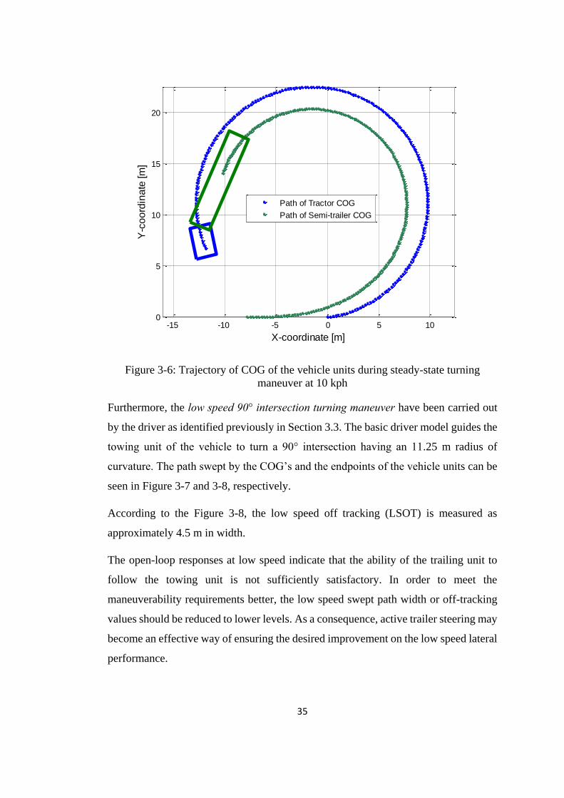
35
-15 -10 -5 0 5 100
5
10
15
20
X-coordinate [m]
Y-c
oo
rdin
ate
[m
]
Path of Tractor COG
Path of Semi-trailer COG
Figure 3-6: Trajectory of COG of the vehicle units during steady-state turning
maneuver at 10 kph
Furthermore, the low speed 90° intersection turning maneuver have been carried out
by the driver as identified previously in Section 3.3. The basic driver model guides the
towing unit of the vehicle to turn a 90° intersection having an 11.25 m radius of
curvature. The path swept by the COG’s and the endpoints of the vehicle units can be
seen in Figure 3-7 and 3-8, respectively.
According to the Figure 3-8, the low speed off tracking (LSOT) is measured as
approximately 4.5 m in width.
The open-loop responses at low speed indicate that the ability of the trailing unit to
follow the towing unit is not sufficiently satisfactory. In order to meet the
maneuverability requirements better, the low speed swept path width or off-tracking
values should be reduced to lower levels. As a consequence, active trailer steering may
become an effective way of ensuring the desired improvement on the low speed lateral
performance.

36
-10 -5 0 5 10 15 20 25 30 35
0
5
10
15
20
25
30
35
40
X-coordinate [m]
Y-c
oo
rdin
ate
[m
]
Figure 3-7: The path of the COG’s of the tractor and semi-trailer during 90-degree
turn at 10 kph
-15 -10 -5 0 5 10 15 20 25 30 35
0
5
10
15
20
25
30
35
40
X-coordinate [m]
Y-c
oo
rdin
ate
[m
]
Figure 3-8: The path of the axle endpoints of the tractor and semi-trailer units during
90-degree turn at 10 kph

37
3.5.2 High Speed Characteristics of Tractor and Semi-trailer Combination
After examining the low speed characteristics of the AHV’s, high speed behavior of
the tractor and semi-trailer combination is investigated in this section. In most cases,
articulated heavy vehicles are used to transport goods and materials on highways. As
a result of this, AHV’s have generally subjected to high speed driving conditions. Lane
changes and turning of large radius curvatures are the two typical maneuvers that the
AHV experience at high speed situations.
As indicated in Section 2.3, the standard maneuver for high speed lane change of
longer combination vehicles are simulated at 88 km/h with a tractor steering input
identified as follows:
𝛿1(𝑡) = 𝐴 𝑠𝑖𝑛 (2𝜋
𝑇𝑡) (3.38)
In equation (3.38), the frequency of the sinusoidal input is standardized in the literature
as 0.4 Hz, corresponding to a period of 2.5 seconds. Amplitude of the tractor steering
input has been chosen in such a way that the minimum lateral acceleration at the front
axle of the towing unit should be 0.15g. In this case, the peak amplitude of the steering
input is chosen as 2 degrees, whereas the vehicle longitudinal speed is set to 88 km/h.
The outcome of the simulations in response to the described maneuver is illustrated in
the following figures (Figure 3-9, Figure 3-10, Figure 3-11).
According to the simulations, the rearward amplification ratio (RWA) is measured as
1.138, while the transient state off-tracking (TOT) value equals to 0.113 m.
Furthermore, high speed steady state off-tracking (HSOT) is observed as 0.093 m in
response to a standard high speed constant radius turn maneuver, in which the driver
steering input is similar to the Equation 3.37.
The lateral movements of the towing and trailing units are not experienced
simultaneously. The reason for this can be identified as follows: The lateral tire forces
are developed on the tractor unit almost immediately in response to the driver steering
action. On the other hand, the required lateral forces on semi-trailer tires cannot be
generated until a side slip motion occurs. Since the lateral tire forces depend directly

38
on the slip angles, the situation can easily be noticed by looking at the timing of slip
angle generation in Figure 3-9.
0 1 2 3 4 5 6 7-3
-2
-1
0
1
2
3
4
Time [s]
Slip
An
gle
s(d
eg
)
1st axle
2nd axle
3rd axle
4th axle
5th axle
Figure 3-9: Slip angles generated by the tires on each axle of the tractor and semi-
trailer combination during standard lane change maneuver
According to the Figure 3-9, there is a time lag between the development of slip angles
on tractor (1st and 2nd) tires and semi-trailer (3rd, 4th and 5th) tires.
The time lag between the force generation lead to the amplification on the lateral
acceleration of the trailing unit. As seen in the Figure 3-10, the lateral acceleration of
the trailing unit follows that of towing unit after some time delay, with greater peak
values. According to Figure 3-11, an overshoot is seen in the path of the semi-trailer
COG, deteriorating the path-following ability.
To conclude, the main problem at high speed conditions can be said as the
amplification of the lateral acceleration. Active trailer steering (ATS) systems can be
serve the purpose of meeting the safety requirements by suppressing the RWA and
improving path-following ability.

39
0 1 2 3 4 5 6 7-0.4
-0.3
-0.2
-0.1
0
0.1
0.2
0.3
Time [s]
La
tera
l a
cce
lera
tio
n [g
]
tractor
semi-trailer
Figure 3-10: Lateral accelerations at the COG’s of tractor and semi-trailer units at
standard lane change maneuver
-1 0 1 2 3 4 5 6 7-0.5
0
0.5
1
1.5
2
2.5
3
3.5
Time [s]
Y-c
oo
rdin
ate
[m
]
Tractor
Semi-trailer
Figure 3-11: The paths of the COG’s of tractor and semi-trailer units at standard lane
change maneuver

40

41
CHAPTER 4
CONTROL STRATEGIES
Several kinds of control strategies are suggested in the literature, some of which are
briefly introduced in Chapter 2. In this study, a new ATS control strategy effective at
both low and high speed cases is proposed and compared with a number of the
described ATS systems.
In this chapter, the theory behind the ATS strategies is examined in detail. Some of
these methods are adjusted to be compatible with the comparison requirements of the
current study. In the following, the list of active trailer steering approaches that are
used in this study is provided:
Steer Ratio Principle (SR)
Command Steering Based Active Optimal Control (ACS)
Virtual Driver Steering Control (VD)
Lateral Position Deviation Preview Control (LPDP)
Lead-Unit Following Control (LUF)
Steer ratio (SR) principle is the most basic control strategy and have been investigated
in the literature for a long time. The second control strategy is similar to a passive
trailer steering system known as command steering. VD and LPDP approaches can be
identified as path-following type of ATS systems. The last strategy is based on the
time lag approach, aiming the trailing unit and the lead unit to follow the same yaw
characteristics. Although the first and second control strategies can be considered as
42
classical ones in the literature, the remaining approaches have been investigated more
recently. In general, the previous approaches focuses on the low speed lateral
performance of AHV’s and are effective in that speed range. The new strategies, on
the other hand, are designed to enhance mostly the high speed lateral performance.
Therefore, the selection of both old and new approaches gives opportunity to compare
the proposed method with strategies that are operational at both low and high speed
conditions.
All of the explained control strategies can be implemented to the vehicle model
obtained in Chapter 3 with a change in the state space matrices as follows:
�̇� = 𝐴𝒙 + 𝐵𝛿1 + 𝐵𝑢𝑢 (4.1)
In the above expression, the conventional vehicle is turned into an AHV whose trailer
wheels are steered actively. The only difference in the state-space form is the addition
of the control input 𝑢, which represents the active steering angles of the semi-trailer
unit and the corresponding control matrix, 𝐵𝑢. The term 𝛿1 represents the steering
action to the tractor unit performed by the driver. Remaining terms indicate the same
variables as in equation (3.26). Further details about the state space matrices for each
control method are given in Appendix C.
In order to simplify the optimal control matrices and adjust the weightings easily, the
three axles of the semi-trailer are combined to a virtual single axle. Then, the active
steering input becomes:
𝑢 = 𝛿𝑠 (4.2)
In other words, the terms 𝛿1 and 𝛿𝑠 in equation (4.1) correspond to the tractor steering
input given by the driver and the active trailer steering input determined by optimal
controller, respectively.
In this study, the driver steering input is known for the standard test conditions whereas
trailer steering angles are unknown quantities. The aim of all the control strategies is
to determine the proper value of that active steering angles so that the lateral
performance of the AHV is improved accordingly.

43
Before proceeding to examine the implementation of active trailer steering, it is
necessary to explain the optimal control theory that will be used for the control
strategies other than SR principle. As explained in the literature survey chapter, linear
quadratic regulator (LQR) technique is the most commonly used control method in the
study of active trailer steering. This is because the LQR offers a practical and
convenient way of control as well as introducing superior performance.
According to the optimal control theory, the design of control system is usually
associated with the choice of a control vector 𝑢 minimizing a predetermined
performance index. For a system described in equation (4.1), a quadratic performance
index is written as follows:
𝐽 = ∫ (𝑥𝑇𝑄𝑥 + 𝑢𝑇𝑅𝑢)∞
0
𝑑𝑡 (4.3)
where both of the Q and R matrices should be positive definite Hermitian or real
symmetric matrices. For the performance index given by (4.3), the quadratic cost
function yields linear control laws that can be identified with the following expression:
𝑢 = −𝐾𝑥 (4.4)
In equation (4.4), the optimal gain matrix 𝐾 is defined as
𝐾 = 𝑅−1𝐵𝑇𝑃 (4.5)
where the symmetric and positive definite matrix P is obtained with the algebraic
Riccati equation given in equation (4.6):
𝐴𝑇𝑃 + 𝑃𝐴 − 𝑃𝐵𝑅−1𝐵𝑃 + 𝑄 = 0 (4.6)
In the optimal control theory, the selection of weighting factors is a vital procedure. In
this study, the weighting factors are determined by looking at the responses obtained
with each active steering control strategy. For each test maneuver, the weighting of
ATS strategies that provides the best performance measure is calculated by using a
trial-error approach.

44
4.1 STEER RATIO PRINCIPLE (SR)
Steer ratio principle is the most basic type of the active steering strategy that was
introduced in 1980s for 4WS passenger cars. The control method was also used in the
study of articulated heavy vehicles [33][34]. In the most recent studies, Rangavajhula
and Tsao investigated the effect of different steer ratios on the lateral performance of
articulated heavy vehicles.
The control method is based on the fundamental idea of making the active trailer
steering in proportional to the tractor front wheel angle. Therefore, the control strategy
is written as the following basic formula:
𝛿𝑠 = 𝜇 𝛿1 (4.7)
where the terms 𝛿𝑠, 𝛿1 and 𝜇 refer to active trailer steering angle, tractor front wheel
steering angle applied by the driver, and the proportionality constant, respectively.
The most important concern of this control strategy is to determine the proportionality
constant connecting the two steering angles. In most cases, the term 𝜇 is defined in a
way such that the steady state side slip angle of the corresponding vehicle unit equals
to zero. Since the system matrix of the vehicle model depends on the vehicle forward
speed, there must be a unique proportionality constant for a specific vehicle speed. As
a result, system matrices given by equation (3.26) should be solved by applying the
zero side slip criteria in steady state conditions.
Figure 4-1 illustrates the change of the steer ratio with respect to the vehicle forward
speed.

45
0 50 100 150 200 250-0.5
0
0.5
1
1.5
2
Vehicle Longitudinal Speed [kph]
Ste
er
Ra
tio
Steer Ratio
Figure 4-1: Steer ratio as a function of vehicle longitudinal speed
Because of large matrix sizes of the state space system, the steer ratios are calculated
using MATLAB® program. The implementation of SR principle requires the
following state space form:
�̇� = 𝑨𝒙 + 𝑩𝛿1 + 𝑩𝒖𝑢 (4.8)
where the control input 𝑢 equals to the active trailer steering input defined in equation
(4.9) as follows:
𝑢 = 𝜇 𝛿1 (4.9)
Note that the corresponding proportionality constant for specific vehicle speed can be
obtained by observing the steer ratios given in Figure 4-1. The details of the matrices
associated with the control strategy are given in Appendix C.
4.2 COMMAND STEERING BASED ACTIVE OPTIMAL CONTROL (ACS)
In this section, a command steering based active trailer steering strategy is
investigated. In classical passive command steering approach, a mechanism is directly
used to produce trailer steering action in proportion to articulation angle between the

46
units. The active type of command steering utilizes the same principal with the use of
optimal control and varying proportionality. Rangavajhula and Tsao suggested the
command steering based active optimal control strategy, comparing its performance
with the classical command steering [5]. In their study, tractor with three full-trailer
combinations is modeled to investigate the behavior at low and medium speed
conditions. The basic geometrical relation used for the determination of each trailer
steering angles in their study is illustrated in Figure 4-2.
Figure 4-2: Active command steering geometry for multiple full-trailers
In the research conducted by Rangavajhula and Tsao, the active steering angles for
each of the full-trailers are expressed as a function of hitch angles between the adjacent
vehicle units. Afterwards, the active steering angles are replaced with the
corresponding hitch angles on their optimal controller. In this study, the same approach
is adopted for a tractor and semi-trailer model. The derivation procedure of the optimal
controller is as follows:

47
First of all, the geometrical relation is expressed as in the following equation.
𝛿𝑠 = 𝛽 𝜓 (4.10)
In equation (4.10), 𝛽 is determined by the geometrical relation, and 𝜓 stands for the
articulation angle between the adjacent vehicle units.
In the method of active command steering, the state-space system given by equation
(4.1) turns out to be the equation (4.11):
�̇� = 𝑨𝒙 + 𝑩𝛿1 + 𝑩𝑨𝑪𝑺𝑢 (4.11)
where the control input, in that case, is the command steering based articulation angle
given by equation (4.12):
𝑢 = 𝜓 (4.12)
In their work, Rangavajhula and Tsao minimize the states of the system while
satisfying minimum control energy criterion. An identity matrix is used for the
weighting of Q matrix in their study. This indicates that all the states of their system
have the same importance. Therefore, the use of equally important states is
investigated in this study, too. The performance index given by equation (4.3) is
directly used in the research with appropriate weighting factor of active steering angle,
giving the best lateral performance.
4.3 VIRTUAL DRIVER STEERING CONTROLLER (VD)
In recent studies, path-following type of control strategies becomes widespread.
Virtual driver steering controller was proposed by Cebon et al. [14]. In this strategy,
the authors assume that a virtual driver sitting at the rear end of the trailing unit aims
to follow the path of the articulation point. In other words, by using active trailer
steering, the virtual driver guides the vehicle aiming the rear end of the semi-trailer to
pass through the route of the fifth wheel. As a result, the major purpose of this control
strategy is to minimize the corresponding path-tracking error. An illustration of virtual
driver steering controller approach is given in Figure 4-3.

48
Figure 4-3: Virtual driver steering controller suggested by Cebon et al. [14]
Obviously, follow point at the trailing unit passes from the lead point after some time.
This requires keeping the path information of the lead point in the memory.
In this study, the approach is adopted with the modification of system matrices so that
the resultant states of the system become as equation (4.13):
𝒙𝑽𝑫 = [𝑣 𝑣𝑡 𝑟 𝑟𝑡 𝑝 𝑝𝑡 𝜙 𝜙𝑡 𝑦𝑒 𝑦5𝑡ℎ 𝑦5𝑡ℎ𝛥 … 𝑦5𝑡ℎ𝑚𝛥]𝑇 (4.13)
In the above expression, first 8 terms correspond to the original system states, whereas
the other terms are related to the lateral position of the fifth wheel, lateral position of
semi-trailer rear end, and the lateral positions of the fifth wheel at previous times,
respectively.
The system matrices are manipulated by using forward difference formula as in
reference [3]. The lateral velocity of the fifth wheel can be described with respect to
the coordinate system fixed to the center of gravities of the vehicle units as in the
following equation:
�̇�5𝑡ℎ(𝑡) = 𝑣(𝑡) − 𝑙𝑓𝑟(𝑡) (4.14)
In a similar way, the lateral velocity of the rear end of the trailing unit can be written
as in the expression given below:
�̇�𝑒(𝑡) = 𝑣𝑡(𝑡) − 𝑙5𝑟𝑡(𝑡) (4.15)

49
In addition to this, the points where the fifth wheel passed at the previous time can be
stored by using forward difference formula with appropriate time step.
�̇�5𝑡ℎ𝑖(𝑡 − 𝑖𝛥) =1
𝛥[𝑦5𝑡ℎ(𝑡 − (𝑖 − 1)𝛥) − 𝑦5𝑡ℎ(𝑡 − 𝑖𝛥)] (4.16)
where 𝑖 = 1,2,3… ,𝑚 and 𝛥 = (𝑙𝑓𝑡 + 𝑙5)/𝑈.
Using the equations (4.14), (4.15) and (4.16), the final state-space system is derived
with the states given by equation (4.13), where the details of the matrices are given in
Appendix C.
In their study, the authors aim to minimize the path-following error that can be written
by equation (4.17). The error is defined as the lateral difference between the path of
the fifth wheel maintained in the memory and path of the rear end of the semi-trailer.
𝑒(𝑡) = 𝑦5𝑡ℎ𝑚𝛥(𝑡) − 𝑦𝑒(𝑡) (4.17)
As a result, the quadratic performance index related to the path-tracking error
minimization via virtual driver steering controller is defined as follows:
𝐽 = ∫ 𝜌1[𝑒(𝑡)]2
∞
0
+ 𝜌2[𝛿𝑠(𝑡)]2 𝑑𝑡 (4.18)
In the expression above, the terms 𝜌1 and 𝜌2 corresponds to the weighting factors
associated with the path-tracking error and the active steering input, respectively.
4.4 LATERAL POSITION DEVIATION PREVIEW (LPDP)
As another type of path-following strategy, lateral position deviation preview
suggested by Islam and He [3] is a similar approach to virtual driver steering control
system. The major difference between the control strategies is the selection of lead and
follow point.
For LPDP controller, the path of the tractor front axle center should be followed by
the semi-trailer axle centers. Figure 4.3 illustrates the approach used in the study of
Islam and He [3].

50
Figure 4-4: Lateral position deviation preview (LPDP) approach suggested by Islam
and He[3]
In this case, the preview path information of the tractor front end is maintained as a
state variable so that the rear axle passes through this path with a time delay. The
approach is adopted with the modification of matrices, yielding the resultant states of
the system be as follows:
𝒙𝑳𝑷𝑫𝑷 = [𝑣 𝑣𝑡 𝑟 𝑟𝑡 𝑝 𝑝𝑡 𝜙 𝜙𝑡 𝑦𝑟 𝑦𝑓 𝑦𝑓𝛥 … 𝑦𝑓𝑛𝛥]𝑇 (4.19)
In the expression written above, the additional states 𝑦𝑓 and 𝑦𝑟 are related to the lateral
positions of tractor front axle center and semi-trailer active axle center. Also, the
remaining states are associated with the positions of tractor front axle center,
considering the time delay.
In order to construct the state-space system, the supplementary equations are written.
For instance, the lateral velocity of the front axle center is described with respect to
the coordinate system fixed to the center of gravity of tractor:
�̇�𝑓(𝑡) = 𝑣(𝑡) + 𝑙1𝑟(𝑡) (4.20)

51
Similarly, the lateral velocity at the rearmost axle center with respect to the coordinate
system fixed to the COG of the semi-trailer is written as in the expression (4.21):
�̇�𝑟(𝑡) = 𝑣𝑡(𝑡) − 𝑙3𝑟𝑡(𝑡) (4.21)
Moreover, the lateral positions passed by the front axle center at previous times are
maintained as state variables by using forward difference formula with suitable time
step.
�̇�𝑓(𝑡 − 𝑗𝛥) =1
𝛥[𝑦𝑓(𝑡 − (𝑗 − 1)𝛥) − 𝑦𝑓(𝑡 − 𝑗𝛥)] (4.22)
where 𝑗 = 1,2,3… , 𝑛 and 𝛥 = (𝑙1 + 𝑙𝑓 + 𝑙𝑓𝑡 + 𝑙𝑡)/𝑈.
After explaining the constructed state-space representation, it is necessary to identify
the corresponding performance index that will be used for the linear quadratic
regulator. The purpose of Islam and He in their paper was to minimize the cost function
related to the lateral position deviation between the units. Using the same approach,
the lateral position error is defined by equation (4.23) for our case:
𝑒(𝑡) = 𝑦𝑓𝑛𝛥(𝑡) − 𝑦𝑟(𝑡) (4.23)
As a result, the quadratic performance index associated with the minimization of
lateral position error is defined as follows:
𝐽 = ∫ 𝜌1[𝑒(𝑡)]2
∞
0
+ 𝜌2[𝛿𝑠(𝑡)]2 𝑑𝑡 (4.24)
It can be noticed that the quadratic performance index is the same as the one used in
the previous control method. On the other hand, the definition of the error for the two
control method is different, resulting in dissimilar responses in the simulations.
4.5 LEAD-UNIT FOLLOWING CONTROLLER (LUF)
Being proposed by Kharazzi [9], lead-unit following controller offers a characteristic-
following approach different from the other control methods. In this control strategy,
the target of the trailing unit is to track the yaw characteristics of the towing unit of an
articulated heavy vehicle with a certain time lag.

52
In the research conducted by Kharazzi [9], the mechanism behind the time-lag
phenomenon is defined as follows:
First of all, the driver of the articulated vehicle performs the steering action leading to
the lateral motion of the towing unit. This lateral motion produces a lateral force on
the articulation joint between the vehicle units. Then, the process is followed by the
yaw motion and side slip of the trailing unit. After the sufficient side slip, the slip
angles of the tires reach a certain level, generating large enough lateral tire forces to
regulate the yaw motion of the trailing unit.
Figure 4-5 illustrates the flowchart explaining the dynamics of the force generation on
the trailing units in response to the driver steering input.
Figure 4-5: Dynamic flowchart of the lateral and yaw motion of the AHV units [9]
It is noticed by examining the Figure 4-5 that the red lines indicating the active steering
input is another variable effecting the generation of the lateral tire forces on the towed
unit axles.

53
In the study, the author indicates that if the time delay between the driver steering input
and the force generation on semi-trailer axles lessen, suppression of the rearward
amplification can be achieved.
According to the study, the lateral tire force to control the yaw motion of the trailing
units can be produced earlier with the implementation of active steering on the trailer
wheels. As a result of this, rearward amplification can be suppressed before the yaw
rates of the towed unit become large. Furthermore, off-tracking problem can be solved
by generating the lateral tire forces with active steering rather than side slip of the
vehicle unit.
In order to implement this approach to the proposed vehicle model, the original state
equations are adjusted. In that case, the states of the system become as follows:
𝒙𝑳𝑼𝑭 = [𝑣 𝑣𝑡 𝑟 𝑟𝑡 𝑝 𝑝𝑡 𝜙 𝜙𝑡 𝑟𝛥 … 𝑟𝑘𝛥]𝑇 (4.25)
In the above expression, the additional states represent the yaw rate characteristics of
the leading unit with the implementation of time lag approach.
Using forward difference formula, the corresponding differential equation can be
expressed as follows:
�̇�(𝑡 − 𝑖𝛥) =1
𝛥[𝑟(𝑡 − (𝑖 − 1)𝛥) − 𝑟(𝑡 − 𝑖𝛥)] (4.26)
where 𝑖 = 1,2,3… , 𝑘
In this case, the approximate time delay is obtained by averaging the yaw difference
between the units of the conventional AHV.
In the lead-unit following case, the error is the difference between the yaw
characteristics of the semi-trailer unit at the present time and that of tractor unit at a
specific previous time.
𝑒(𝑡) = 𝑟𝑡(𝑡) − 𝑟𝑘𝛥(𝑡) (4.27)
Therefore, the quadratic performance index offering the minimization of
characteristic-following error is written as follows:
54
𝐽 = ∫ 𝜌1[𝑒(𝑡)]2
∞
0
+ 𝜌2[𝛿𝑠(𝑡)]2 𝑑𝑡 (4.28)
In the expression above, the terms 𝜌1 and 𝜌2 correspond to the weighting factors
associated with the error and the active steering input, respectively.
4.6 PROPOSED CONTROLLER: LATERAL ACCELERATION
CHARACTERISTICS FOLLOWING (LACF)
Having mentioned different control methods used in the literature, it is time to explain
the control strategy proposed in this study. The newly introduced control method is
called as lateral acceleration characteristics following (LACF). Actually, the suggested
control strategy is based on the time lag approach like the previous method (LUF). On
the other hand, this strategy offers further dominance on the lateral acceleration
characteristics of AHVs at both low and high speed conditions. The expectation from
the proposed controller is improved lateral performance at transient state conditions
additional to steady state conditions.
In the previous method implemented by Kharazzi, the yaw rate characteristic was the
only parameter that the author concerned. However, the lateral acceleration of the
vehicle units are not only dependent on the yaw rates but also influenced by the side-
slip and roll motions of the vehicle. In most general terms, lateral accelerations of the
vehicle units can be defined with the following expressions:
�̈�(𝑡) = �̇�(𝑡) + 𝑈𝑟(𝑡) −𝑚𝑠ℎ
∗
𝑚�̇�(𝑡) (4.29)
�̈�𝑡(𝑡) = �̇�𝑡(𝑡) + 𝑈𝑡𝑟𝑡(𝑡) −𝑚𝑠𝑡ℎ𝑡
∗
𝑚𝑡�̇�𝑡(𝑡) (4.30)
In order to investigate the lateral acceleration characteristic precisely, the vehicle
simulation results given by Figure 3-9 are separated to its effective components. The
overall lateral acceleration of the tractor unit is illustrated together with the
contributions of the three independent motion components in Figure 4-6.

55
0 1 2 3 4 5 6 7-0.4
-0.3
-0.2
-0.1
0
0.1
0.2
0.3
0.4
Time [s]
La
tera
l A
cce
lera
tio
n [g
]
Side Slip Motion
Yaw Motion
Roll Motion
Overall Lateral Acceleration of Tractor
Figure 4-6: Contribution of the side slip, yaw and roll motions on the lateral
acceleration characteristics of tractor unit
It should be noted lateral acceleration of semi-trailer unit is not shown in the figure to
reduce the complexity. In Figure 4-6, it is seen that the side slip and yaw motions are
the dominant components that have large influence on the lateral acceleration
characteristics.
Since the roll degree of freedom have little effect on the lateral acceleration
characteristics of both vehicle units, the equations stated above are reduced to the
following form:
�̈�(𝑡) = �̇�(𝑡) + 𝑈𝑟(𝑡) (4.31)
�̈�𝑡(𝑡) = �̇�𝑡(𝑡) + 𝑈𝑡𝑟𝑡(𝑡) (4.32)
The terms �̇� and 𝑟 are the two important parameters effecting the lateral acceleration
characteristics at transient state and steady state conditions, respectively.

56
The proposed controller has contribution to the previously mentioned lead-unit
following controller, concerning both �̇� and 𝑟 terms. Recall that the only concern of
the lead-unit following control was the yaw characteristics (𝑟).
In order to construct a state-space system that can be utilized for the proposed control
method, the following states are obtained:
𝒙𝑳𝑨𝑪𝑭 = [ 𝒙 �̇� �̇�𝛥… �̇�𝑙𝛥 𝑟𝛥… 𝑟𝑘𝛥 ]𝑇 (4.33)
where the first and second terms represent the original states used on the conventional
vehicle and the derivatives of these states, respectively.
To obtain the derivatives as state variables, the matrix manipulation given by equation
(4.34) is applied:
�̇�𝑳𝑨𝑪𝑭 = [𝑨 𝟎𝟎 𝑨
] 𝒙𝑳𝑨𝑪𝑭 + [𝑩 𝟎𝟎 𝑩
] 𝜹𝟏 + [𝑩𝒖 𝟎𝟎 𝑩𝒖
] 𝒖 (4.34)
Using forward difference formula, the time-delayed states of the system can be
obtained. Then, the corresponding differential equations can be written as in the
equations (4.35) and (4.36):
�̈�(𝑡 − 𝑖𝛥) =1
𝛥[�̇�(𝑡 − (𝑖 − 1)𝛥) − �̇�(𝑡 − 𝑖𝛥)] (4.35)
where 𝑖 = 1,2,3… , 𝑙
�̇�(𝑡 − 𝑖𝛥) =1
𝛥[𝑟(𝑡 − (𝑖 − 1)𝛥) − 𝑟(𝑡 − 𝑖𝛥)] (4.36)
where 𝑖 = 1,2,3… , 𝑘
The approximate time delays are obtained by averaging the yaw difference and side-
slip rate differences between the units of the conventional AHV. The derivation steps
of the state space system for the proposed controller are provided in Appendix C in
detail.

57
Recall that, in the LACF strategy, the lateral acceleration characteristics of the semi-
trailer should track that of the tractor with a time delay between the two units.
Therefore, the error definition in this case is written as in equation (4.37):
𝑒(𝑡) = {�̇�𝑡(𝑡) + 𝑈𝑡𝑟𝑡(𝑡)} − {�̇�𝑛𝛥(𝑡) + 𝑈𝑟𝑚𝛥(𝑡)} (4.37)
The quadratic cost function minimizing the error in the lateral acceleration
characteristics become:
𝐽 = ∫ 𝜌1[𝑒(𝑡)]2
∞
0
+ 𝜌2[𝛿𝑠(𝑡)]2 𝑑𝑡 (4.38)
Then, the error expression is simplified to avoid the non-diagonal elements in the
weighting matrix. This simplification also helps with observing the effect of each
component during weighting factor adjustment. As a result of this, the error is
separated into two components as follows:
𝑒1(𝑡) = �̇�𝑡(𝑡) − �̇�𝑛𝛥(𝑡) (4.39)
𝑒2(𝑡) = 𝑟𝑡(𝑡) − 𝑟𝑚𝛥(𝑡) (4.40)
The resulting quadratic performance index is given in equation (4.41):
𝐽 = ∫ 𝜌1[𝑒1(𝑡)]2 + 𝜌2[𝑒2(𝑡)]
2
∞
0
+ 𝜌3[𝛿𝑠(𝑡)]2 𝑑𝑡 (4.41)
Having identified the state space system and defined the quadratic performance index,
a linear quadratic regulator (LQR) now can be used for the proposed controller.
To summarize, the proposed active trailer steering strategy is a time lag type ATS
strategy, which is a completion of the LUF method. Considering an additional variable,
it is expected to show better performance than LUF method both and low and high
speed conditions. The simulation results and their comparison are presented in the next
chapter.

58

59
CHAPTER 5
SIMULATION RESULTS
In this chapter, the lateral response of the vehicle model to the specified standard test
maneuvers is investigated. MATLAB® platform is used for the vehicle dynamic
simulations. The relevant standard maneuvers stated in the literature survey chapter
are used to test the lateral performance associated with each active strategy. The
comparison of the performances of ATS strategies is provided.
The standard maneuvers introduced in the study of lateral performance evaluation are
explained in the previous chapters. In this study, the most popular test maneuvers are
utilized for the assessment of the lateral performance of the modeled articulated
vehicle. At high and low vehicle speed conditions, the applied maneuvers are
summarized as in the following table:
Table 5-1: Summary of standard maneuvers implemented for the simulation
STANDARD
MANEUVER TYPE
DRIVER STEERING
INPUT
VEHICLE
FORWARD SPEED
Low Speed Constant Radius
Turning Maneuver
Ramped Step Steering
Input 10 km/h
Low Speed 90° Intersection
Turning Maneuver
Driver Model Steering
Input 10 km/h
High Speed Constant
Radius Turning Maneuver
Ramped Step Steering
Input 100 km/h
High Speed Lane Change
Maneuver Sinusoidal Steering Input 88 km/h

60
In the following sections, the high speed and low speed cases are investigated
separately. The performance evaluation of the articulated vehicle controlled with
active trailer steering strategies is provided.
5.1 LATERAL PERFORMANCE OF THE AHV AT LOW SPEED
CONDITIONS
Articulated heavy vehicles are generally used in highways at medium to high forward
speed situations. On the other hand, narrow local roads and parking conditions bring
about the necessity of sufficient lateral performance of the AHVs at low speeds.
As stated in literature survey section, the low speed performance of an AHV is
evaluated at 10 km/h, turning an 11.25 m radius of curvature circle in steady state
conditions. Therefore, a ramped step steering input with an amplitude providing the
specified constant radius is used in the simulations. Figure 5.1 illustrates the ramped
step steering input associated with the low speed turning maneuver.
0 2 4 6 8 10 12 14 16 18 200
2
4
6
8
10
12
14
16
18
Time [s]
Ste
eri
ng
In
pu
t [d
eg
ree
s]
Ramped Step Input Applied by the Driver
Figure 5-1: Steering input applied by the driver during low speed 360° constant
radius turn

61
In this standard test maneuver, it can be noticed that the amplitude of the driver steering
input goes up to 16 degrees due to the turning of small radius of curvature. Such large
steering inputs are reasonable and non-problematic because of the very low vehicle
longitudinal speeds.
The performance evaluation in this maneuver is carried out with the determination of
the low speed circle swept path width (SPW). The steady state circle SPW is defined
as the lateral position deviation between the paths of the COG’s of each unit.
Therefore, the difference between the steady state turning radii of the two units give
the expression related to the specified performance measure. Equation (5.1) is used to
determine the value of low speed circle steady state SPW at the indicated test
condition.
𝑆𝑃𝑊 = 𝑅𝑡 − 𝑅𝑠 (5.1)
where the terms 𝑅𝑡 and 𝑅𝑠 refers to the turning radii of tractor and semitrailer units
after both units reached the steady state conditions, respectively.
Due to the imposed large driver steering angles, the vehicle dynamic simulations are
expected to give huge SPW values at low speed maneuvers. After implementing all of
the control strategies stated in Chapter 4, responses to the standard low speed 360°
constant radius turning test maneuver are summarized in Table 5-2.
Table 5-2: SPW values obtained by the simulations for each control strategy
Conv. SR ACS VD LPDP LUF LACF
SPW 2.432 m 1.651 m 2.100 m 2.243 m 2.297 m 0.013 m 0.008 m
Initial
Error zero zero zero zero zero 0.982 m 0.990 m
As can be inferred from the Table 5-2, the LUF and the proposed LACF control
strategies behave better in terms of steady-state off-tracking performance at the
expense of some position error in the initial path. Furthermore, the recently used path-
following methods, VD and LPDP, provides unsatisfactory results compared to the

62
steer ratio principle (SR) and active command steering (ACS). This is because the new
methods are generally interested in the high speed lateral performance whereas the old
strategies mainly focus on low speed conditions.
-10 -5 0 5 10 15
0
5
10
15
20
X-coordinate [m]
Y-c
oo
rdin
ate
[m
]
Desired Path
Conventional
SR
ACS
VD
LUF
LACF
Figure 5-2: Trajectories of the semi-trailer unit at low speed circle turning maneuver
for each control strategy
The low speed circle turning trajectory of the semi-trailer units for each control
strategy is illustrated in Figure 5-2. It should be noted that the desired path is the
collection of points from which the center of gravity of the towing unit passes. Despite
the initial error, the LUF and LACF methods entail very successful steady-state circle
SWP performance.
Similar to the low speed steady state circle swept path width, low speed 90°
intersection turn has to be performed at a longitudinal speed of 10 km/h. Also, the
corresponding radius of curvature should be 11.25 m [18].
In the simulations, the basic driver model indicated in Chapter 3 drives the articulated
heavy vehicle so that an intersection turn is achieved. Different from the other

63
maneuvers, the steering input for the tractor front axle is determined by the driver
model in that case. Figure 5-3 illustrates the corresponding steering input which is
generated by the basic driver model.
0 5 10 15 20 250
5
10
15
20
25
30
35
40
Time [s]
Ste
eri
ng
In
pu
t [d
eg
ree
s]
Figure 5-3: Steering input applied by the driver during low speed 90° intersection
turn maneuver
During the specified maneuver, the assessment of the vehicle lateral performance has
been performed by measuring the path swept by the endpoints of vehicle units. In the
simulations, the paths of the left side of the rearmost axle of the semi-trailer have been
kept in the memory as well as the path of the right side of the front axle of the tractor.
Afterwards, the maximum difference between the swept path is identified as the low
speed off-tracking (LSOT) value, given by the equation below:
𝐿𝑆𝑂𝑇 = 𝑚𝑎𝑥(𝑅𝑡𝑟 − 𝑅𝑠𝑙) (5.2)
Table 5-3: The LSOT values obtained by the simulations for each control strategy
Con SR ACS VD LPDP LUF LACF
LSOT 4.76 m 4.37 m 4.75 m 4.76 m 4.76 m 4.20 m 4.16 m

64
-15 -10 -5 0 5 10 15 20 25 30 35
0
5
10
15
20
25
30
35
40
X-coordinate [m]
Y-c
oo
rdin
ate
[m
]
Tractor
Conventional
SR
ACS
VD
LUF
LACF
Figure 5-4: The area swept by the endpoints of the vehicle units during 90°
intersection turn maneuver at low speed
10 15 20 25 30
0
2
4
6
8
10
12
14
16
18
X-coordinate [m]
Y-c
oo
rdin
ate
[m
]
Tractor
Conventional
SR
ACS
VD
LUF
LACF
Figure 5-5: Zoomed view of the swept area by the vehicle units during 90°
intersection turn maneuver at low speed

65
The LSOT results of the simulation are illustrated in Table 5.3 above. According to
the results, proposed LACF method and LUF approach provide better results among
the other strategies. In addition, steer ratio principle can be said as satisfactory when
compared to the other methods. Remaining control strategies result in almost no
change in the low speed off-tracking performance of the articulated heavy vehicle.
The area swept by the left side of the semi-trailer rearmost axle and the right side of
the tractor front axle is illustrated in Figure 5-4 and Figure 5-5.
5.2 LATERAL PERFORMANCE OF THE AHV AT HIGH SPEED
CONDITIONS
Most of the time, articulated heavy vehicles is exposed to high speed driving
conditions on highways, especially in the steady state turning and lane change
maneuvers. Therefore, a suitable design of the longer combination vehicles at high
speed situations becomes vital for the efficiency and safety issues. That is the reason
for the recent trend in the field: the active trailer steering control strategies to be
designed for high speed conditions.
In high speed cases, there are two commonly used standard maneuvers to evaluate the
lateral acceleration performance of the AHVs, which are the high speed turning
maneuvers and the high speed lane changes. As explained in the Chapter 2, the
important performance measures in the range of high forward speeds are the steady
state high speed off-tracking (HSOT), transient state high-speed off-tracking (TOT)
and rearward amplification ratio (RWA).
According to the standard maneuvers used in the literature, high-speed steady state
off-tracking is evaluated at the speed of 100 km/h when the tractor front axle center of
follows the circle of 393 m radius [17]. A ramped step steering input is implemented
by the driver to the tractor front wheels. Figure 5.6 shows the corresponding steering
input applied by the driver.

66
0 2 4 6 8 10 12 14 16 18 200
0.2
0.4
0.6
0.8
1
1.2
1.4
Time [s]
Ste
eri
ng
In
pu
t [d
eg
ree
s]
Ramped Step Input Applied by the Driver
Figure 5-6: Steering input applied by the driver during high speed 360° constant
radius turn
Different from the low speed constant circle turning maneuver, the steering angles
implemented by the driver are smaller in that case. This is because the AHV turns very
large radius of curvature at high forward speeds. Regarding such large radius of
curvatures and small steering action, it can be implied that the vehicle combination is
subjected to the situations that is somewhat near to straight ahead driving condition.
As a result, the high speed off-tracking (HSOT) values obtained from the simulations
are expected to be smaller compared to the low speed conditions. The HSOT values is
calculated with the following expression:
𝐻𝑆𝑂𝑇 = 𝑅𝑡 − 𝑅𝑠 (5.3)
Table 5-4: The HSOT values obtained by the simulations for each control strategy
Con SR ACS VD LPDP LUF LACF
HSOT 0.093 m 0.010 m 0.055 m 0.016 m 0.030 m 0.022 m 0.022 m

67
According to the table illustrated above, almost all of the control strategies provide
satisfactory results in terms of HSOT, except the active command steering. Proposed
LACF method is among the one of the most effective strategies, whereas the best
approaches are the steer ratio principle and virtual driver steering controller.
The second and the most frequently used driving situation for the AHV is the high
speed lane change maneuver. Having been clarified in the literature survey chapter,
the standard lane change maneuver is investigated using the following maneuver
identified by Fancher and Winkler [4]: A sinusoidal wave steering input should be
applied by the driver to the front axle of the towing unit at a constant forward speed of
88 km/h. The frequency of the wave has to be 0.4 Hz, whereas the lane change
maneuver produces a minimum 0.15g lateral acceleration at the front axle of the tractor
unit.
According to the specified maneuvers, the following steering input is applied by the
driver in the vehicle simulations:
0 1 2 3 4 5 6 7-2
-1.5
-1
-0.5
0
0.5
1
1.5
2
Time [s]
Ste
eri
ng
In
pu
t [d
eg
ree
s]
Driver Sinusoidal Steering Input
Figure 5-7: Driver steering input during lane change maneuver at 88 kph

68
From the specified lane change maneuver, two different lateral performance measure
is obtained by the simulations. In fact, rearward amplification ratio (RWA) is an
important lateral performance measure as well as the high speed transient off-tracking
(TOT). The simulations yield the values of RWA and TOT, which are defined as in
the following equations:
𝑅𝑊𝐴 =𝑝𝑒𝑎𝑘(�̈�𝑠)
𝑝𝑒𝑎𝑘(�̈�𝑡) (5.4)
𝑇𝑂𝑇 = 𝑝𝑒𝑎𝑘(𝑦𝑠) − 𝑝𝑒𝑎𝑘(𝑦𝑡) (5.5)
The active trailer steering control strategies aim to reduce the TOT as much as
possible, while suppressing the RWA to unity. In the literature, the RWA implies
increased roll stability near to the value of unity.
Different from the other standard maneuvers, two independent lateral performance
measures are taken during high speed lane change maneuver, which are RWA and
TOT. As a consequence, the adjustment of the weighting factors leads to various
combinations of RWA and TOT pairs. In general, the designer prefers appropriate
weighting factors regarding his own concerns. Showing the trade-off relationship
between RWA and TOT values on a map (see Figure 5-8) helps the designer to observe
all possibilities to be chosen.
According to the Figure 5-8, the most successful control strategies in terms of path-
following are VD, LPDP, and LACF since the high speed transient off-tracking (TOT)
is almost reduced to zero. Furthermore, VD, LPDP, LUF, and LACF methods can
suppress the rearward amplification (RWA) to its ideal level of unity.

69
0.7 0.8 0.9 1 1.1 1.2 1.30
0.02
0.04
0.06
0.08
0.1
0.12
Rearward Amplification Ratio
Hig
h S
pe
ed
Off-t
rackin
g [m
]
ACS
VD
LPDP
LUF
LACF
Figure 5-8: HSOT and RWA map showing the trade-off relationship associated with
the changing weight factors
Table 5-5 is constructed using the responses obtained from the vehicle dynamic
simulation during high speed lane change maneuver. Note that the RWA and TOT pair
corresponds to the weighting factors for minimum off-tracking case, while RWA* and
TOT* is obtained with the weighting factors for the ideal amplification level.
Table 5-5: Rearward amplification (RWA) and transient off-tracking (TOT) values
obtained by the simulations for each control strategy
Con SR ACS VD LPDP LUF LACF
RWA 1.138 1.675 1.090 0.961 0.895 0.978 0.953
TOT 0.113 m 0.110 m 0.084 m zero zero 0.042 m zero
RWA* 1.138 1.675 1.090 1.000 1.000 1.000 1.000
TOT* 0.113 m 0.110 m 0.084 m 0.024 m 0.045 m 0.056 m 0.043 m

70
According to the Table 5-5, the control strategies VD, LPDP and LACF behave well
among the others, almost zeroing the transient path-following off-tracking of the
tractor and semi-trailer combination. Although the SR principle has almost no effect
on the transient off-tracking performance, LUF and ACS methods make improvement
in the reduction of TOT. Likewise, the path-following type controllers VD & LPDP
and the time-lag type controllers LUF and LACF suppresses the rearward
amplification ratio below the unity.
The path where the COG’s of tractor and semi-trailer units follows during high speed
lane change is illustrated in Figure 5-5. To examine the path-following errors correctly,
zoomed view of the upper and lower parts of the figure are provided (see Figure 5-6
and Figure 5-7).
Having observed the bottom part of the vehicle paths, the SR strategy seems to be
unsatisfactory at tracking the towing unit. Looking at the zoomed view of the top, on
the other hand, enhanced path-following ability of VD, LPDP, and LACF are justified.
-1 0 1 2 3 4 5 6 7-0.5
0
0.5
1
1.5
2
2.5
3
3.5
Time [s]
Y-c
oo
rdin
ate
[m
]
Desired Path
Conventional semi-trailer
SR semi-trailer
ACS semi-trailer
VD semi-trailer
LPDP semi-trailer
LUF semi-trailer
LACF semi-trailer
Figure 5-9: Lateral paths of the COGs of the vehicle units during high speed lane
change maneuver

71
-0.5 0 0.5 1 1.5 2
-0.2
0
0.2
0.4
0.6
0.8
1
Time [s]
Y-c
oo
rdin
ate
[m
]
Desired Path
Conventional semi-trailer
SR semi-trailer
ACS semi-trailer
VD semi-trailer
LPDP semi-trailer
LUF semi-trailer
LACF semi-trailer
Figure 5-10: Zoomed bottom view of the lateral paths of the COGs of the vehicle
units during high speed lane change maneuver
1.5 2 2.5 3 3.5 4
2.6
2.7
2.8
2.9
3
3.1
3.2
3.3
3.4
Time [s]
Y-c
oo
rdin
ate
[m
]
Desired Path
Conventional semi-trailer
SR semi-trailer
ACS semi-trailer
VD semi-trailer
LPDP semi-trailer
LUF semi-trailer
LACF semi-trailer
Figure 5-11: Zoomed top view of the lateral paths of the COGs of the vehicle units
during high speed lane change maneuver

72
Figure 5-12 and Figure 5-13 illustrate the lateral acceleration and yaw velocity
characteristics of the vehicle units, respectively. According to the Figure 5-12, the
lateral acceleration of semi-trailer unit tries to follow the tractor lateral acceleration
characteristics with a time lag for LACF strategy. Consequently, suppressed RWA and
less off-tracking due to the non-oscillatory behavior are verified. The non-oscillatory
behavior is also observed in the yaw characteristics and articulation angle given by
Figure 5-13 and Figure 5-14.
Similar to the proposed control strategy, LPDP, VD, and LUF also accomplish the
suppression of RWA, while ACS is not sufficient in that performance measure. Note
that the results obtained with the SR principle are not shown in Figure 5-12, since the
large amplitudes hide other variations on the figure.
0 1 2 3 4 5 6 7-0.4
-0.3
-0.2
-0.1
0
0.1
0.2
0.3
Time [s]
La
tera
l a
cce
lera
tio
n [g
]
Tractor
conventional
ACS
VD
LPDP
LUF
LACF
Figure 5-12: Lateral accelerations at the COGs of the vehicle units during high speed
lane change maneuver

73
0 1 2 3 4 5 6 7-10
-8
-6
-4
-2
0
2
4
6
8
10
Time [s]
Ya
w v
elo
city[d
eg
/s]
Tractor
Conventional
SR
ACS
VD
LPDP
LUF
LACF
Figure 5-13: Yaw velocities at the COGs of the vehicle units during high speed lane
change maneuver
0 1 2 3 4 5 6 7-4
-3
-2
-1
0
1
2
3
4
Time [s]
Hitch
An
gle
[de
gre
e]
Conventional
SR
ACS
VD
LPDP
LUF
LACF
Figure 5-14: Articulation angle between the tractor and semi-trailer during high
speed lane change maneuver

74
In addition, Figure 5-15 illustrates the roll angles during the high speed lane change
maneuver. The proposed LACF strategy makes improvement on the oscillatory
characteristics of the roll angles. All the strategies except the SR and ACS provide
satisfactory roll behavior that may be seen as an indication of the enhanced roll
characteristics.
Table 5-6: Peak roll angles values obtained for each control strategy
Con SR ACS VD LPDP LUF LACF
Peak
Roll
Angle
0.8503° 1.063° 0.8564° 0.8186° 0.7845° 0.7900° 0.8364°
0 1 2 3 4 5 6 7
-1
-0.8
-0.6
-0.4
-0.2
0
0.2
0.4
0.6
0.8
1
Time [s]
Ro
ll A
ng
les [d
eg
]
Tractor Unit
Conventional
SR
ACS
VD
LPDP
LUF
LACF
Figure 5-15: Roll angles of the vehicle units during high speed lane change maneuver

75
Table 5-7: Lateral performance measures obtained for each control strategy
Measure Control Strategy
Conv. SR ACS VD LPDP LUF LACF
SPW 2.432 m 1.651 m 2.100 m 2.243 m 2.297 m 0.013 m 0.008 m
Initial
SPW
zero zero zero zero zero 0.982 m 0.990 m
LSOT 4.76 m 4.37 m 4.75 m 4.76 m 4.76 m 4.20 m 4.16 m
RWA 1.138 1.675 1.090 0.961 0.895 0.978 0.953
RWA* 1.138 1.675 1.090 1.000 1.000 1.000 1.000
TOT 0.113 m 0.110 m 0.084 m zero zero 0.042 m zero
TOT* 0.113 m 0.110 m 0.084 m 0.024 m 0.045 m 0.056 m 0.043 m
HSOT 0.093 m 0.010 m 0.055 m 0.016 m 0.030 m 0.022 m 0.022 m
Table 5-7 summarizes the lateral performance measures obtained for the applied
control strategies. The vehicle dynamic simulations provide the following conclusions:
Steer ratio (SR) behaves well at low forward speeds, whereas its high speed
lateral performance is not good enough compared to the conventional AHV.
However, the control strategy gives the best response in terms of high speed
off-tracking and provides successful response in terms of low speed swept path
width.
Among the strategies, active command steering (ACS) provides an average
performance in terms of combined low and high speed conditions. Although
all the performance measures are improved by the implementation of ACS, the
effect of the improvement is not sufficient. Indeed, there are alternative
strategies that improve each of the performance measures to a greater extent.
76
The path-following types of control methods, VD and LPDP, provide superior
response at high speed test conditions. In fact, VD controller gives the best
overall high speed performance among all the strategies. The weakness of these
methods, on the other hand, is the poor lateral performance they offer at low
forward speeds.
By looking at the values of RWA*, it is concluded that VD, LPDP, LUF and
LACF can suppress the rearward amplification to its ideal level. The
adjustment of weighting factors results in a RWA* ratio of unity. In this case,
however, the corresponding transient off-tracking TOT* values deteriorate.
Lead unit following (LUF) strategy provides sufficient performance at both
low and high speed situations, giving the second best results among the control
strategies, after LACF. One weakness of LUF and LACF is the initial error in
the SPW during low speed turning test conditions. However, this initial error
causes increased steady state circle turning performance.
The weakness of LUF strategy in transient state can directly be seen by looking
at the TOT value. While the other path-following types and the proposed
control strategy can reduced the off-tracking to zero, LUF strategy is not
sufficiently successful.
Proposed control strategy, LACF, is more successful than the existing
strategies when evaluated on the basis of combined overall low and high speed
performance. The control strategy gives the best response in terms of SPW,
LSOT, and TOT. Furthermore, HSOT and RWA values are close to the best
values obtained in the simulations.

77
CHAPTER 6
CONCLUSION
The aim of this study is to design an active trailer steering control strategy for
articulated heavy vehicles. Among the various combinations of towing and trailing
vehicle units, a combination consisting of a tractor and a multi-axle semi-trailer is
selected for this study. The selected combination is the most commonly used type of
the AHV. In order to prevent the unstable motion modes, which are jack-knifing, trailer
swing, and roll over; lateral performance of the AHV should meet certain criteria. A
number of active trailer steering systems have been proposed in the literature to
improve the performance of AHV.
When the dynamic models of AHV used in the literature are examined in detail, it is
noted that each model has its positive and negative characteristic features depending
on the application considered. After reviewing these models, a 5 DOF nonlinear
yaw/roll dynamic model of a tractor and multi-axle semi-trailer combination was
developed for this study.
The ATS control strategy proposed in this study is based on the Lead Unit Following
(LUF) control method. LUF has been implemented such that the yaw velocity of the
trailing unit follows the yaw velocity of the tractor. The main feature of the proposed
strategy, Lateral Acceleration Characteristic Following (LACF) control, is that the
trailing unit tries to follow the lateral acceleration characteristics of the towing unit
involving both the side slip acceleration and the yaw velocity of the towing unit rather
than just the yaw velocity. Thus the trailing unit is effectively following the lateral
acceleration of the towing unit.
78
In order to evaluate the lateral performance of an AHV controlled by the proposed
method, a couple of classical and a couple of more recent strategies in the literature
are implemented. Simulations using these strategies and the proposed strategy with the
standard test conditions have been performed. Then the results from the simulations
are compared to assess the performance of each strategy.
The simulation results reveal that the existing strategies do not consistently provide
satisfactory lateral performance when both low and high speeds are considered. The
classical steer ratio (SR) strategy provides good performance with respect to off-
tracking both at low and high speeds. However, its performance with respect to
rearward amplification is not satisfactory at high speeds. Active command steering
(ACS) strategy results in probably the poorest overall performance among the
strategies included in the analyses at low and high speeds. On the other hand, the
virtual driver (VD) and lateral position deviation preview (LPDP) show better
performance generally in high speed conditions than low speed conditions. Therefore
they are more suited for high speeds. The lead unit following method (LUF) may
provide the best performance for combined low and high speed conditions when
compared to the strategies analyzed above even though the VD strategy is superior
with respect to high speed behavior. The proposed strategy LACF is shown to provide
better performance when both low and high speed behavior are taken into account
among all the strategies. Its superiority is due to the fact that it can provide a much
faster response in transient off-tracking conditions as well as better path following
ability.
To summarize, an active trailer steering control strategy, Lateral Acceleration
Characteristic Following LACF, is designed for a tractor and multi-axle semi-trailer
combination. The lateral performance of the vehicle combination is enhanced with the
implementation of the proposed active trailer steering strategy. The basic superiority
of the proposed method with respect to major classical and recent control strategies is
its performance when both low and high speed behavior are concerned.
The study detailed in the thesis study may be improved by using a more sophisticated
model for the tractor semi-trailer combination. In particular the use of non-linear tire
79
models would make it possible to apply a wider range of weighting factors so that the
limiting cases without considering the linearity assumptions. Further, the proposed
controller can be implemented on different combinations of AHVs. As a result, the
success and limitations of the LACF controller can be verified on various vehicle
configurations. A set of weighting factors as a function of forward speed of the
combination may also be searched for an adaptive application of the strategy.

80

81
REFERENCES
[1] OECD, Moving Freight with Better Trucks: Improving Safety, Productivity and
Sustainability. OECD Publishing, 2011.
[2] I. Knight, T. Robinson, B. Robinson, T. Barlow, I. McCrae, A. Odhams, R. L.
Roebuck, and C. Cheng, “The likely effects of permitting longer semi-trailers
in the UK: vehicle specification, performance and safety,” TRL Publ. Proj.,
2010.
[3] M. M. Islam and Y. He, “Design of a Preview Controller for Articulated Heavy
Vehicles,” J. Mech. Eng. Autom., vol. 3, pp. 661–676, 2013.
[4] P. Fancher and C. Winkler, “Directional performance issues in evaluation and
design of articulated heavy vehicles,” Veh. Syst. Dyn., vol. 45, no. 7–8, pp. 607–
647, 2007.
[5] K. Rangavajhula and H.-S. J. Tsao, “Command steering of trailers and
command-steering-based optimal control of an articulated system for tractor-
track following,” Proc. Inst. Mech. Eng. Part D J. Automob. Eng., vol. 222, no.
6, pp. 935–954, 2008.
[6] X. Ding, Y. He, J. Ren, and T. Sun, “A Comparative Study of Control
Algorithms for Active Trailer Steering Systems of Articulated Heavy
Vehicles,” Am. Control Conf., pp. 3617–3622, 2012.
[7] Z. Tianjun and Z. Changfu, “Modelling and active safe control of heavy tractor
semi-trailer,” 2nd Int. Conf. Intell. Comput. Technol. Autom. ICICTA, vol. 2,
pp. 112–115, 2009.
[8] A. Hac, D. Fulk, and H. Chen, “Stability and Control Considerations of Vehicle-
Trailer Combination,” SAE Int. J. Passeng. Cars - Mech. Syst., no. 724, pp. 776–
790, 2008.
[9] S. Kharrazi, “Steering based lateral performance control of long heavy vehicle
combinations,” 2012.
[10] S. H. Tamaddoni, “Yaw Stability Control of Tractor Semi-Trailers,” 2008.

82
[11] Z. Tianjun, S. Xiaojun, and Z. Changfu, “Development of a Tractor-Semitrailer
Stability,” Int. Conf. Power Electron. Intell. Transp. Syst., pp. 102–105, 2009.
[12] S. H. Tabatabaei Oreh, R. Kazemi, and S. Azadi, “A new desired articulation
angle for directional control of articulated vehicles,” Proc. Inst. Mech. Eng. Part
K J. Multi-body Dyn., 2012.
[13] D. Oberoi, “Enhancing roll stability and directional performance of articulated
heavy vehicles based on anti-roll control and design optimization.,” 2011.
[14] C. Cheng, R. Roebuck, A. Odhams, and D. Cebon, “High-speed optimal
steering of a tractor–semitrailer,” Veh. Syst. Dyn. Int. J. Veh. Mech. Mobil.,
2011.
[15] M. Manjurul Islam, “Parallel Design Optimization of Multi-Trailer Articulated
Heavy Vehicles with Active Safety Systems Md . Manjurul Islam,” 2013.
[16] S. H. Tabatabaei Oreh, R. Kazemi, and S. Azadi, “A sliding mode controller for
directional control of articulated vehicles,” Proc. Inst. Mech. Eng. Part K J.
Multi-body Dyn., 2012.
[17] F. Distribution, M. Using, and S. Grids, “Performance Standards for Heavy
Vehicles in Australia,” 2001.
[18] B. Jujnovich and D. Cebon, “Comparative Performance of Semi-trailer
Steering,” Int. Symp. Heavy Veh. Weight. Dimens., 2002.
[19] P. LeBlanc, M. El-Gindy, and J. Woodrooffe, “Self-Steering Axles: Theory and
Practice.” 1989.
[20] R. L. Nisonger and C. C. Macadam, “Influence of Self-steering Axles on the
Directional Response of Commercial Vehicles,” Veh. Syst. Dyn. Int. J. Veh.
Mech. Mobil., pp. 289–291, 2002.
[21] S. Luo, “Relative Performance Analysis of Articulated Vehicles with Multiple
Conventional Liftable and Self-steering Axles,” 2004.
[22] S. Sankar, S. Rakheja, and A. Piche, “Directional Dynamics of a Tractor-
Semitrailer with Self and Forced-Steering Axles.” 1991.
[23] B. Özkan, E. Aptoula, T. Heren, H. Mandacı, and Ç. Can, “Minimization of Tire
Wear for Tractor Semi-trailers with Command Steering,” Otomotiv Teknol.
Kongresi, pp. 1–8, 2014.
[24] H. W. J. Onkhoff and O. F. Begkenham, “Automatic Steering Device For
Swiveling Bogies,” 1932.

83
[25] H. W. Jonkhoff, “Bogie Vehicle Steering Mechanism,” 1937.
[26] C. S. Abbott, “Steering Mechanism for Trucks and Trailers,” 1933.
[27] H. Prem, L. Mai, and K. Atley, “Application of Trackaxle to Multi-Combination
Vehicles,” 2006.
[28] H. Prem and E. Ramsey, “Performance evaluation of the Trackaxle Self-
Steering System,” Int. Symp. Heavy Veh. Weight. Dimens., pp. 405–422, 2002.
[29] B. Jujnovich and D. Cebon, “Validation of a semi-trailer steering model,” Int.
Symp. Heavy Veh. Weight. Dimens., 2004.
[30] A. Percy and I. Spark, “A numerical control algorithm for a B-double truck-
trailer with steerable trailer wheels and active hitch angles,” Proc. Inst. Mech.
Eng. Part D J. Automob. Eng., vol. 226, no. 3, pp. 289–300, 2012.
[31] M. M. Islam, “Design synthesis of articulated heavy vehicles with active trailer
steering systems,” 2010.
[32] S. H. T. Oreh, R. Kazemi, S. Azadi, and A. Zahedi, “A New Method for
Directional Control of a Tractor Semi-trailer,” vol. 6, no. 12, pp. 396–409, 2012.
[33] D. H. Wu and J. Hai, “Analysis of dynamic lateral response for a multi-axle-
steering tractor and trailer,” Int. J. Heavy Veh. Syst., vol. 10, no. 4, p. 281, 2003.
[34] D.-H. Wu, “A theoretical study of the yaw/roll motions of a multiple steering
articulated vehicle,” Proc. Inst. Mech. Eng. Part D J. Automob. Eng., vol. 215,
no. 12, pp. 1257–1265, 2005.
[35] K. Rangavajhula and H. S. J. Tsao, “Effect of multi-axle steering on off-tracking
and dynamic lateral response of articulated tractor-trailer combinations,” Int. J.
Heavy Veh. Syst., vol. 14, no. 4, p. 376, 2007.
[36] I. Notsu, S. Takahashi, and Y. Watanabe, “Investigation into Turning Behaviour
of Semi-trailer with Additional Trailer-wheel Steering.” 1991.
[37] B. A. Jujnovich and D. Cebon, “Path-Following Steering Control for
Articulated Vehicles,” J. Dyn. Syst. Meas. Control, vol. 135, no. 3, 2013.
[38] R. Roebuck, A. Odhams, K. Tagesson, C. Cheng, and D. Cebon,
“Implementation of trailer steering control on a multi-unit vehicle at high
speeds,” J. Dyn. Syst. Meas. Control, vol. 136, no. 2, p. 021016, 2013.
[39] B. Jujnovich, R. Roebuck, A. Odhams, and D. Cebon, “Implementation of
active rear steering of a tractor-semi-trailer,” 2007.
84
[40] A. M. C. Odhams, R. L. Roebuck, B. A. Jujnovich, and D. Cebon, “Active
steering of a tractor-semi-trailer,” Proc. Inst. Mech. Eng. Part D J. Automob.
Eng., vol. 225, no. 7, pp. 847–869, 2011.
[41] A. M. C. Odhams, R. L. Roebuck, D. Cebon, and C. B. Winkler, “Dynamic
safety of active trailer steering systems,” Proc. Inst. Mech. Eng. Part K J. Multi-
body Dyn., vol. 222, no. 4, pp. 367–380, 2008.
[42] X. Ding, S. Mikaric, and Y. He, “Design of an active trailer-steering system for
multi-trailer articulated heavy vehicles using real-time simulations,” Proc. Inst.
Mech. Eng. Part D J. Automob. Eng., 2012.
[43] M. M. Islam, X. Ding, and Y. He, “A closed-loop dynamic simulation-based
design method for articulated heavy vehicles with active trailer steering
systems,” Veh. Syst. Dyn., vol. 50, no. 5, pp. 675–697, 2012.
[44] S. Kharrazi, M. Lidberg, R. Roebuck, J. Fredriksson, and A. Odhams,
“Implementation of active steering on longer combination vehicles for
enhanced lateral performance,” Veh. Syst. Dyn., no. July 2015, pp. 1–22, 2012.
[45] S. Kharrazi, M. Lidberg, and J. Fredriksson, “A generic controller for improving
lateral performance of heavy vehicle combinations,” Proc. Inst. Mech. Eng.
Part D J. Automob. Eng., 2012.
[46] G. Isiklar and I. Besselink, “Simulation of complex articulated commercial
vehicles for different driving manoeuvres,” 2007.

85
APPENDIX A
VEHICLE MODEL
Figure A-1: Vehicle model of a tractor and semi-trailer combination
In order to obtain the lateral response of the vehicle during specific maneuvers, a
proper implementation of the vehicle model is essential. Figure 1A illustrates the
bicycle model of the articulated heavy vehicle including the roll degree of freedom.
To derive the necessary AHV model, Newton 2nd law of dynamics are used. In the
Figure 1A, a body centered coordinate system is fixed to the center of gravity of each

86
vehicle unit, assuming that all the masses of the tractor and semi-trailer are lumped at
that points. Either side of the AHV have brought together at the centerline to represent
the combination as a bicycle model. In other words, the right and left tires are
represented as only one wheel, considering the overall cornering stiffness being equal
to the total stiffness of all the wheels on the same axle.
Note that the steering angles and slip angles of the wheels are denoted as 𝛿𝑖 and 𝛼𝑖 for
the ith axle of the vehicle, respectively. The corresponding longitudinal-lateral-yaw
velocities at the COG points of the vehicle units are described as 𝑢, 𝑣, 𝑟 and 𝑢𝑡, 𝑣𝑡, 𝑟𝑡
in their positive x-y-z directions.
The relevant lengths between the axles or articulation points are expressed as 𝑙𝑖 ,
whereas the tire forces at the ith axle are written as 𝐹𝑥𝑖 and 𝐹𝑦𝑖 .
For all the other variables and symbols, looking at the Nomenclature section will help.
Figure A-2: The reaction forces created at the vehicle articulation point
Illustration of the vehicle combination as separate vehicle units will help us to easily
obtain the equations of motions for tractor and semi-trailer. As a result, the reaction
force at the articulation point should act to each unit as an action-reaction pair. Figure
A2 reveals the forces at the hitch point of the vehicle.

87
After the separation, the equations of motions for the tractor can be identified as the
following equations. According to the Figure A1, the full expressions of force and
moment equilibrium in both translational and rotational directions is written using
Newton 2nd law as follows:
𝑚(�̇� − 𝑣𝑟) +𝑚𝑠(ℎ∗𝑟𝑝) = −𝐹𝑦1𝑠𝑖𝑛𝛿1 + 𝐹𝑥1𝑐𝑜𝑠𝛿1 + 𝐹𝑥2 + 𝐹𝑥𝑓 (𝐴1)
𝑚(�̇� + 𝑈𝑟) − 𝑚𝑠(ℎ∗�̇�) = 𝐹𝑦1𝑐𝑜𝑠𝛿1 + 𝐹𝑥1𝑠𝑖𝑛𝛿1 + 𝐹𝑦2 + 𝐹𝑦𝑓 (𝐴2)
𝐼𝑧𝑧�̇� − 𝐼𝑠𝑥𝑧�̇� = 𝑙1(𝐹𝑦1cos𝛿1 + 𝐹𝑥1sin𝛿1) − l2Fy2 − l𝑓F𝑦𝑓 (A3)
𝐼𝑥𝑥�̇� − 𝐼𝑥𝑧�̇� − 𝑚𝑠ℎ∗(�̇� + 𝑈𝑟)
= 𝑚𝑠𝑔ℎ∗𝑠𝑖𝑛𝜙 − (∑𝐾𝜙)𝜙 − (∑𝐶𝜙)p − ℎ𝑓𝑟F𝑦𝑓 + 𝐾12(ϕ𝑡 − ϕ) (A4)
Note that the Equation (A4) stands for the motion about the roll degree of freedom of
the tractor unit.
Similarly, the equation of motions for the semi-trailer can be written as follows:
𝑚𝑡(�̇�𝑡 − 𝑣𝑡𝑟𝑡) + 𝑚𝑠𝑡(ℎ𝑡∗𝑟𝑡𝑝𝑡)
= −𝐹𝑥𝑓𝑐𝑜𝑠𝛹 + 𝐹𝑦𝑓𝑠𝑖𝑛𝛹 + 𝐹𝑥3𝑐𝑜𝑠𝛿3 + 𝐹𝑥4𝑐𝑜𝑠𝛿4 + 𝐹𝑥5𝑐𝑜𝑠𝛿5
+ 𝐹𝑦3𝑠𝑖𝑛𝛿3 + 𝐹𝑦4𝑠𝑖𝑛𝛿4 + 𝐹𝑦5𝑠𝑖𝑛𝛿5 (𝐴5)
𝑚𝑡(�̇�𝑡 + 𝑈𝑡𝑟𝑡) − 𝑚𝑠𝑡(ℎ𝑡∗𝑝�̇�)
= −𝐹𝑥𝑓𝑠𝑖𝑛𝛹 − 𝐹𝑦𝑓𝑐𝑜𝑠𝛹 − 𝐹𝑥3𝑠𝑖𝑛𝛿3 − 𝐹𝑥4𝑠𝑖𝑛𝛿4 − 𝐹𝑥5𝑠𝑖𝑛𝛿5
+ 𝐹𝑦3𝑐𝑜𝑠𝛿3 + 𝐹𝑦4𝑐𝑜𝑠𝛿4 + 𝐹𝑦5𝑐𝑜𝑠𝛿5 (𝐴6)
𝐼𝑧𝑧𝑡�̇�𝑡 − 𝐼𝑠𝑥𝑧𝑡𝑝�̇�
= 𝑙3(𝐹𝑥3𝑠𝑖𝑛𝛿3 − 𝐹𝑦3𝑐𝑜𝑠𝛿3) + 𝑙4(𝐹𝑥4𝑠𝑖𝑛𝛿4 − 𝐹𝑦4𝑐𝑜𝑠𝛿4)
+ l5(𝐹𝑥5𝑠𝑖𝑛𝛿5 − 𝐹𝑦5𝑐𝑜𝑠𝛿5) − 𝑙𝑓𝑡𝐹𝑦𝑓cos𝛹 − 𝑙𝑓𝑡𝐹𝑥𝑓𝑠𝑖𝑛𝛹 (𝐴7)
𝐼𝑥𝑥𝑡𝑝�̇� − 𝐼𝑥𝑧𝑡𝑟�̇� −𝑚𝑠𝑡ℎ𝑡∗(𝑣�̇� + 𝑈𝑡𝑟𝑡)
= 𝑚𝑠𝑡𝑔ℎ𝑡∗𝑠𝑖𝑛𝜙𝑡 − (∑𝐾𝜙𝑡)𝜙𝑡 − (∑𝐶𝜙𝑡)p𝑡 + ℎ𝑓𝑟𝑡𝐹𝑦𝑓cos𝛹
+ ℎ𝑓𝑟𝑡𝐹𝑥𝑓𝑠𝑖𝑛𝛹 − 𝐾12(ϕ𝑡 −ϕ) (A8)

88
Additionally, the lateral and longitudinal velocities at the articulation point of the AHV
should be compatible. Equations (A9) and (A10) refers to the velocity expressions of
semi-trailer derived with the help of the constraint at the hitch point.
𝑈𝑡 = 𝑈𝑐𝑜𝑠𝛹 − 𝑣𝑠𝑖𝑛𝛹 + 𝑙𝑓𝑟𝑠𝑖𝑛𝛹 (𝐴9)
𝑣𝑡 = 𝑈𝑠𝑖𝑛𝛹 + 𝑣𝑐𝑜𝑠𝛹 − 𝑙𝑓𝑟𝑐𝑜𝑠𝛹 − 𝑙𝑓𝑡𝑟𝑡 − ℎ𝑓𝑟𝑝 + ℎ𝑓𝑟𝑡𝑝𝑡 (𝐴10)
The derivatives of the above expressions will be used to convert the differential
equations to a state space model. Therefore, a differentiation procedure has been
applied to express the equations as follows:
�̇�𝑡 = �̇�𝑐𝑜𝑠𝛹 − 𝑈�̇�𝑠𝑖𝑛𝛹 − �̇�𝑠𝑖𝑛𝛹 − 𝑣�̇�𝑐𝑜𝑠𝛹 + 𝑙𝑓�̇�𝑠𝑖𝑛𝛹 + 𝑙𝑓𝑟�̇�𝑐𝑜𝑠𝛹 (𝐴11)
�̇�𝑡 = �̇�𝑠𝑖𝑛𝛹 + 𝑈�̇�𝑐𝑜𝑠𝛹 + �̇�𝑐𝑜𝑠𝛹 − 𝑣�̇�𝑠𝑖𝑛𝛹 − 𝑙𝑓�̇�𝑐𝑜𝑠𝛹 + 𝑙𝑓𝑟�̇�𝑠𝑖𝑛𝛹 − 𝑙𝑓𝑡�̇�𝑡
− ℎ𝑓𝑟�̇� + ℎ𝑓𝑟𝑡𝑝�̇� (𝐴12)
Since the fundamental research subject is the lateral performance of the AHV in the
dissertation, the major consideration of the model have been the motion of the vehicle
combination in y-direction. Hence, the tractive & braking effects can be neglected to
simplify the vehicle model i.e. x-components of the forces are not regarded in the
expressions from (A1) to (A8). After the elimination of Equations (A1) and (A5) and
the effects of longitudinal forces, the resultant expressions reduced to the following
form:
𝑚(�̇� + 𝑈𝑟) − 𝑚𝑠(ℎ∗�̇�) = 𝐹𝑦1𝑐𝑜𝑠𝛿1 + 𝐹𝑦2 + 𝐹𝑦𝑓 (𝐴13)
𝐼𝑧𝑧�̇� − 𝐼𝑠𝑥𝑧�̇� = 𝑙1[𝐹𝑦1cos𝛿1] − l2Fy2 − l𝑓F𝑦𝑓 (A14)
(𝐼𝑥′𝑥′)�̇� − 𝐼𝑥′𝑧′�̇� − 𝑚𝑠ℎ∗(�̇� + 𝑈𝑟)
= 𝑚𝑠𝑔ℎ∗𝜙 − (∑𝐾𝜙)𝜙 − (∑𝐶𝜙)p − F𝑦𝑓ℎ𝑓𝑟 + 𝐾12(ϕ𝑡 −ϕ) (A15)
𝑚𝑡(�̇�𝑡 + 𝑈𝑡𝑟𝑡) − 𝑚𝑠𝑡(ℎ𝑡∗𝑝�̇�)
= −𝐹𝑦𝑓𝑐𝑜𝑠𝛹 + 𝐹𝑦3𝑐𝑜𝑠𝛿3 + 𝐹𝑦4𝑐𝑜𝑠𝛿4 + 𝐹𝑦5𝑐𝑜𝑠𝛿5 (𝐴16)

89
−𝐼𝑠𝑥𝑧𝑡𝑝�̇� + 𝐼𝑧𝑧𝑡�̇�𝑡
= 𝑙3[−𝐹𝑦3𝑐𝑜𝑠𝛿3] + 𝑙4[−𝐹𝑦4𝑐𝑜𝑠𝛿4] + l5[−𝐹𝑦5𝑐𝑜𝑠𝛿5]
− 𝑙𝑓𝑡𝐹𝑦𝑓cos𝛹 (𝐴17)
(𝐼𝑥𝑥𝑡)𝑝�̇� − 𝐼𝑥𝑧𝑡𝑟�̇� −𝑚𝑠𝑡ℎ𝑡∗(𝑣�̇� + 𝑈𝑡𝑟𝑡)
= 𝑚𝑠𝑡𝑔ℎ𝑡∗𝑠𝑖𝑛𝜙𝑡 − (∑𝐾𝜙𝑡)𝜙𝑡 − (∑𝐶𝜙𝑡)p𝑡 + 𝐹𝑦𝑓ℎ𝑓𝑟𝑡
− 𝐾12(ϕ𝑡 − ϕ) (A18)
In order to convert the identified equations of motions to a state-space system, all the
terms should be replaced by the state variables. At first, the lateral force 𝐹𝑦𝑖’s on the
above expressions is written in terms of corresponding slip angles and cornering
stiffness as follows:
𝐹𝑦𝑖 = 𝐶𝑠𝑖𝑡ℎ 𝑎𝑥𝑙𝑒𝛼𝑖 = 𝐶𝑖𝛼𝑖 (𝐴19)
For further details, the full expressions of the slip angle 𝛼𝑖’s are written as the
following equations from (A20) to (A24):
𝛼1 = tan−1 (
𝑣 + 𝑙1𝑟
𝑈) − 𝛿1 (𝐴20)
𝛼2 = tan−1 (
𝑣 − 𝑙2𝑟
𝑈) (𝐴21)
𝛼3 = tan−1 (
𝑣𝑡 − 𝑙3𝑟𝑡𝑈𝑡
) + 𝛿3 (𝐴22)
𝛼4 = tan−1 (
𝑣𝑡 − 𝑙4𝑟𝑡𝑈𝑡
) + 𝛿4 (𝐴23)
𝛼5 = tan−1 (
𝑣𝑡 − 𝑙5𝑟𝑡𝑈𝑡
) + 𝛿5 (𝐴24)
For the above equations, the sign convention related to the slip angles are denoted as
follows: When going from centerline of the wheel to direction of motion, clockwise
rotation means positive slip angle whereas counter-clockwise rotation refers to
negative slip angle.

90
In order to decrease the level of complexity of the model for the controller design,
small angle assumptions have been used for the linearization of the vehicle model.
According to the assumption, steering angles, slip angles and hitch angles are
considered as very small so that the equations (A25) and (A26) can be written in that
case.
sin(𝛿) = 𝛿 ≅ 0 & cos(𝛿) = 1 (𝐴25)
sin(𝛹) = 𝛹 ≅ 0 & cos(𝛹) = 1 (𝐴26)
Also, the slip angles have been reduced to the following form:
𝛼1 =𝑣 + 𝑙1𝑟
𝑈− 𝛿1 (𝐴27)
𝛼2 =𝑣 − 𝑙2𝑟
𝑈 (𝐴28)
𝛼3 =𝑣𝑡 − 𝑙3𝑟𝑡𝑈𝑡
+ 𝛿3 (𝐴29)
𝛼4 =𝑣𝑡 − 𝑙4𝑟𝑡𝑈𝑡
+ 𝛿4 (𝐴30)
𝛼5 =𝑣𝑡 − 𝑙5𝑟𝑡𝑈𝑡
+ 𝛿5 (𝐴31)
Furthermore, the linearization of the velocity compatibility equations and their
derivatives are written as follows:
Then,
𝑈𝑡 = 𝑈 − 𝑣𝛹 + 𝑙𝑓𝑟𝛹 (𝐴32)
𝑣𝑡 = 𝑈𝛹 + 𝑣 − 𝑙𝑓𝑟 − 𝑙𝑓𝑡𝑟𝑡 − ℎ𝑓𝑟𝑝 + ℎ𝑓𝑟𝑡𝑝𝑡 (𝐴33)
�̇�𝑡 = �̇� − 𝑈�̇�𝛹 − �̇�𝛹 − 𝑣�̇� + 𝑙𝑓�̇�𝛹 + 𝑙𝑓𝑟�̇� (𝐴34)
�̇�𝑡 = �̇�𝛹 + 𝑈�̇� + �̇� − 𝑣�̇�𝛹 − 𝑙𝑓�̇� + 𝑙𝑓𝑟�̇�𝛹 − 𝑙𝑓𝑡�̇�𝑡 + ℎ𝑓𝑟�̇� − ℎ𝑓𝑟𝑡𝑝�̇� (𝐴35)

91
To avoid the state by state multiplications, products of small variables have been
neglected in the above equations as follows:
𝑈𝑡 = 𝑈 (𝐴36)
𝑣𝑡 = 𝑈𝛹 + 𝑣 − 𝑙𝑓𝑟 − 𝑙𝑓𝑡𝑟𝑡 − ℎ𝑓𝑟𝑝 + ℎ𝑓𝑟𝑡𝑝𝑡 (𝐴37)
�̇�𝑡 = �̇� − 𝑣�̇� + 𝑙𝑓𝑟�̇� (𝐴38)
�̇�𝑡 = 𝑈𝑟 − 𝑈𝑟𝑡 + �̇� − 𝑙𝑓�̇� − 𝑙𝑓𝑡�̇�𝑡 + ℎ𝑓𝑟�̇� − ℎ𝑓𝑟𝑡𝑝�̇� (𝐴39)
In addition to this, it will be helpful to express the geometric relations of the yaw rates
with the articulation angle as Equation (A40):
�̇� = 𝑟 − 𝑟𝑡 (𝐴40)
The reaction forces at the articulation point can be eliminated by combining the tractor
equations of motions with the ones for the semi-trailer unit. After the elimination
procedure, a state-space model is ready to be constructed. The necessary manipulations
on the equations result in overall differential equations related to the state-space model
in terms of state variables. The final form of the equations is given as seen from
equation (A41) to equation (A48):
{𝑚}�̇� + {𝑚𝑡}𝑣�̇� + {−𝑚𝑠ℎ∗}�̇� + {−𝑚𝑠𝑡ℎ𝑡
∗}𝑝�̇�
= {𝐶1 + 𝐶2𝑈
} 𝑣 + {𝐶3 + 𝐶4 + 𝐶5
𝑈} 𝑣𝑡 + {
𝐶1𝑙1 − 𝐶2𝑙2 −𝑚𝑈2
𝑈} 𝑟
+ {−𝐶3𝑙3 − 𝐶4𝑙4 − 𝐶5𝑙5 −𝑚𝑡𝑈
2
𝑈} 𝑟𝑡 + {−𝐶1}𝛿1 + {𝐶3}𝛿3 + {𝐶4}𝛿4
+ {𝐶5}𝛿5 (𝐴41)
{𝑚𝑙𝑓}�̇� + {𝐼𝑧𝑧}�̇� + {−𝐼𝑠𝑥𝑧 −𝑚𝑠ℎ∗𝑙𝑓}�̇�
= {𝐶1𝑙1 − 𝐶2𝑙2 + (𝐶1 + 𝐶2)𝑙𝑓
𝑈}𝑣
+ {𝐶1𝑙1
2 + 𝐶2𝑙22 + (𝐶1𝑙1 − 𝐶2𝑙2 −𝑚𝑈
2)𝑙𝑓𝑈
} 𝑟
+ {−𝐶1(l1 + 𝑙𝑓)}𝛿1 (𝐴42)

92
{𝑚ℎ𝑓𝑟 −𝑚𝑠ℎ∗}�̇� + {−𝐼𝑠𝑥𝑧}�̇� + {𝐼𝑠𝑥𝑥 −𝑚𝑠ℎ
∗ℎ𝑓𝑟}�̇�
= {(𝐶1 + 𝐶2)ℎ𝑓𝑟
𝑈}𝑣 + {
(𝐶1𝑙1 − 𝐶2𝑙2 −𝑚𝑈2)ℎ𝑓𝑟 + 𝑚𝑠𝑈
2ℎ∗
𝑈} 𝑟
+ {−∑𝐶𝜙}𝑝 + 𝑚𝑠ℎ∗𝑔 − ∑𝐾𝜙 − 𝐾12𝜙 + {𝐾12}ϕ𝑡
+ {−𝐶1ℎ𝑓𝑟}𝛿1 (𝐴43)
{−𝑚𝑡𝑙𝑓𝑡}𝑣�̇� + {𝐼𝑧𝑧𝑡}�̇�𝑡 + {𝐼𝑠𝑥𝑧𝑡 +𝑚𝑠𝑡ℎ𝑡∗𝑙𝑓𝑡}𝑝�̇�
= {−𝐶3(𝑙3 + 𝑙𝑓𝑡) − 𝐶4(𝑙4 + 𝑙𝑓𝑡) − 𝐶5(𝑙5 + 𝑙𝑓𝑡)
𝑈} 𝑣𝑡
+ {𝐶3𝑙3
2 + 𝐶4𝑙42 + 𝐶5𝑙5
2 + (𝐶3𝑙3 + 𝐶4𝑙4 + 𝐶5𝑙5 +𝑚𝑡𝑈2)𝑙𝑓𝑡
𝑈} 𝑟𝑡
+ {−𝐶3(𝑙3 + 𝑙𝑓𝑡)}𝛿3 + {−𝐶4(𝑙4 + 𝑙𝑓𝑡)}𝛿4
+ {−𝐶5(𝑙5 + 𝑙𝑓𝑡)}𝛿5 (𝐴44)
{𝑚𝑡ℎ𝑓𝑟𝑡 −𝑚𝑠𝑡ℎ𝑡∗}𝑣�̇� + {−𝐼𝑠𝑥𝑧𝑡}𝑟�̇� + {𝐼𝑠𝑥𝑥𝑡 −𝑚𝑠𝑡ℎ𝑡
∗ℎ𝑓𝑟𝑡}𝑝�̇�
= {(𝐶3 + 𝐶4 + 𝐶5)ℎ𝑓𝑟𝑡
𝑈}𝑣𝑡
+ {−ℎ𝑓𝑟𝑡(𝐶3𝑙3 + 𝐶4𝑙4 + 𝐶5𝑙5 +𝑚𝑡𝑈
2) + 𝑚𝑠𝑡𝑈2ℎ𝑡
∗
𝑈} 𝑟𝑡
+ {−∑𝐶𝜙𝑡}p𝑡 + {𝐾12}ϕ + {𝑚𝑠𝑡ℎ𝑡∗𝑔 − ∑𝐾𝜙𝑡 − 𝐾12}𝜙𝑡 + {𝐶3ℎ𝑓𝑟𝑡}𝛿3
+ {𝐶4ℎ𝑓𝑟𝑡}𝛿4 + {𝐶5ℎ𝑓𝑟𝑡}𝛿5 (𝐴45)
{−1}�̇� + {1}�̇�𝑡 + {𝑙𝑓}�̇� + {𝑙𝑓𝑡}�̇�𝑡 + {−ℎ𝑓𝑟}�̇� + {ℎ𝑓𝑟𝑡}𝑝�̇� = {𝑈}𝑟 + {−𝑈}𝑟𝑡 (𝐴46)
{1}�̇� = {1}𝑝 (𝐴47)
{1}𝜙𝑡̇ = {1}𝑝𝑡 (𝐴48)
In order to construct the mathematical model of the physical vehicle, a linear time
invariant (LTI) state space system of the following form is studied.
�̇�(𝑡) = 𝑨𝒙(𝑡) + 𝑩𝒖(𝑡)
𝒚(𝑡) = 𝑪𝒙(𝑡) + 𝑫𝒖(𝑡)

93
𝒙(𝑡) : state variables vector
𝒚(𝑡) : output variables vector
𝒖(𝑡) : input variables vector
𝑨 : system matrix
𝑩 : input matrix
𝑪 : output matrix
𝑫 : disturbance or feedforward matrix
The following definitions provides the explanations of the 8 states used in the
derivation of the linear yaw & roll articulated vehicle model:
𝒙 = [𝑣 𝑣𝑡 𝑟 𝑟𝑡 𝑝 𝑝𝑡 𝜙 𝜙𝑡 ]𝑇
𝑣 : Lateral velocity of COG of tractor
𝑣𝑡 : Lateral velocity of COG of semi-trailer
𝑟 : Yaw rate of the COG of tractor
𝑟𝑡 : Yaw rate of the COG of semi-trailer
𝑝 : Roll rate of the sprung mass COG of the tractor
𝑝𝑡 : Roll rate of the sprung mass COG of the semi-trailer
𝜙 : Roll angle of the sprung mass COG of the tractor
𝜙𝑡 : Roll angle of the sprung mass COG of the semi-trailer
The equations provided from (A41) to (A48) should be rearranged to have the
following matrix form:

94
[𝐴𝑖]8𝑥8
{
�̇�𝑣�̇��̇�𝑟�̇��̇�𝑝�̇�𝑝𝑝𝑡}
= [𝐵𝑖]8𝑥8
{
𝑣𝑣𝑡𝑟𝑟𝑡𝑝𝑝𝑡𝜙𝜙𝑡}
+ [𝐶𝑖]8𝑥4 {
𝛿1𝛿3𝛿4𝛿5
} (𝐴49)
In the matrices, all the elements are zero except for the ones that are listed as follows:
𝐴𝑖(1,1) = 𝑚
𝐴𝑖(1,2) = 𝑚𝑡
𝐴𝑖(1,5) = −𝑚𝑠ℎ∗
𝐴𝑖(1,6) = −𝑚𝑠𝑡ℎ𝑡∗
𝐴𝑖(2,1) = 𝑚𝑙𝑓
𝐴𝑖(2,3) = 𝐼𝑧𝑧
𝐴𝑖(2,5) = −𝐼𝑠𝑥𝑧 −𝑚𝑠ℎ∗𝑙𝑓
𝐴𝑖(3,1) = 𝑚ℎ𝑓𝑟 −𝑚𝑠ℎ∗
𝐴𝑖(3,3) = −𝐼𝑠𝑥𝑧
𝐴𝑖(3,5) = 𝐼𝑠𝑥𝑥 −𝑚𝑠ℎ∗ℎ𝑓𝑟
𝐴𝑖(4,2) = −𝑚𝑡𝑙𝑓𝑡
𝐴𝑖(4,4) = 𝐼𝑧𝑧𝑡
𝐴𝑖(4,6) = −𝐼𝑠𝑥𝑧𝑡 +𝑚𝑠𝑡ℎ𝑡∗𝑙𝑓𝑡
𝐴𝑖(5,2) = 𝑚𝑡ℎ𝑓𝑟𝑡 −𝑚𝑠𝑡ℎ𝑡∗
𝐴𝑖(5,4) = −𝐼𝑠𝑥𝑧𝑡
𝐴𝑖(5,6) = 𝐼𝑠𝑥𝑥𝑡 −𝑚𝑠𝑡ℎ𝑡∗ℎ𝑓𝑟𝑡

95
𝐴𝑖(6,1) = −1
𝐴𝑖(6,2) = 1
𝐴𝑖(6,3) = 𝑙𝑓
𝐴𝑖(6,4) = 𝑙𝑓𝑡
𝐴𝑖(6,5) = −ℎ𝑓𝑟
𝐴𝑖(6,6) = ℎ𝑓𝑟𝑡
𝐴𝑖(7,7) = 1
𝐴𝑖(8,8) = 1
𝐵𝑖(1,1) =𝐶1 + 𝐶2𝑈
𝐵𝑖(1,2) =𝐶3 + 𝐶4 + 𝐶5
𝑈
𝐵𝑖(1,3) =𝐶1𝑙1 − 𝐶2𝑙2 −𝑚𝑈
2
𝑈
𝐵𝑖(1,4) =−𝐶3𝑙3 − 𝐶4𝑙4 − 𝐶5𝑙5 −𝑚𝑡𝑈
2
𝑈
𝐵𝑖(2,1) =𝐶1𝑙1 − 𝐶2𝑙2 + (𝐶1 + 𝐶2)𝑙𝑓
𝑈
𝐵𝑖(2,3) =𝐶1𝑙1
2 + 𝐶2𝑙22 + (𝐶1𝑙1 − 𝐶2𝑙2 −𝑚𝑈
2)𝑙𝑓𝑈
𝐵𝑖(3,1) =(𝐶1 + 𝐶2)ℎ𝑓𝑟
𝑈
𝐵𝑖(3,2) =(𝐶1𝑙1 − 𝐶2𝑙2 −𝑚𝑈
2)ℎ𝑓𝑟 + 𝑚𝑠𝑈2ℎ∗
𝑈
𝐵𝑖(3,5) = −∑𝐶𝜙
𝐵𝑖(3,7) = 𝑚𝑠ℎ∗𝑔 − ∑𝐾𝜙 − 𝐾12

96
𝐵𝑖(3,8) = 𝐾12
𝐵𝑖(4,2) =−𝐶3(𝑙3 + 𝑙𝑓𝑡) − 𝐶4(𝑙4 + 𝑙𝑓𝑡) − 𝐶5(𝑙5 + 𝑙𝑓𝑡)
𝑈
𝐵𝑖(4,4) =𝐶3𝑙3
2 + 𝐶4𝑙42 + 𝐶5𝑙5
2 + (𝐶3𝑙3 + 𝐶4𝑙4 + 𝐶5𝑙5 +𝑚𝑡𝑈2)𝑙𝑓𝑡
𝑈
𝐵𝑖(5,2) =(𝐶3 + 𝐶4 + 𝐶5)ℎ𝑓𝑟𝑡
𝑈
𝐵𝑖(5,4) =−ℎ𝑓𝑟𝑡(𝐶3𝑙3 + 𝐶4𝑙4 + 𝐶5𝑙5 +𝑚𝑡𝑈
2) + 𝑚𝑠𝑡𝑈2ℎ𝑡
∗
𝑈
𝐵𝑖(5,6) = −∑𝐶𝜙𝑡
𝐵𝑖(5,7) = 𝐾12
𝐵𝑖(5,8) = 𝑚𝑠𝑡ℎ𝑡∗𝑔 − ∑𝐾𝜙𝑡 − 𝐾12
𝐵𝑖(6,3) = 𝑈
𝐵𝑖(6,4) = −𝑈
𝐵𝑖(7,5) = 1
𝐵𝑖(8,6) = 1
𝐶𝑖(1,1) = −𝐶1
𝐶𝑖(1,2) = 𝐶3
𝐶𝑖(1,3) = 𝐶4
𝐶𝑖(1,4) = 𝐶5
𝐶𝑖(2,1) = −𝐶1(l1 + 𝑙𝑓)
𝐶𝑖(3,1) = −𝐶1ℎ𝑓𝑟
𝐶𝑖(4,2) = −𝐶3(𝑙3 + 𝑙𝑓𝑡)
𝐶𝑖(4,3) = −𝐶4(𝑙4 + 𝑙𝑓𝑡)

97
𝐶𝑖(4,4) = −𝐶5(𝑙5 + 𝑙𝑓𝑡)
𝐶𝑖(5,2) = 𝐶3ℎ𝑓𝑟𝑡
𝐶𝑖(5,3) = 𝐶4ℎ𝑓𝑟𝑡
𝐶𝑖(5,4) = 𝐶5ℎ𝑓𝑟𝑡
In the form of standard state space representation, the matrices are expressed as
follows:
�̇� = 𝑨𝒙 + 𝑩𝜹 (𝐴50)
where 𝐴 = [𝐴𝑖]−1[𝐵𝑖] and 𝐵 = [𝐴𝑖]
−1[𝐶𝑖]

98

99
APPENDIX B
VEHICLE DATA
Table B- 1: Vehicle data adapted from reference [5]
SYMBOL EXPLANATION VALUE UNIT
𝑚 Whole mass of the tractor unit 6769 𝑘𝑔
𝑚𝑠 Sprung mass of the tractor unit 4819 𝑘𝑔
𝑚𝑡 Whole mass of the semi-trailer unit 32151 𝑘𝑔
𝑚𝑠𝑡 Sprung mass of the semi-trailer unit 30821 𝑘𝑔
𝐼𝑠𝑥𝑥
Roll moment of inertia of sprung mass
of tractor unit about the COG of its
sprung mass center
4348 𝑘𝑔𝑚2
𝐼𝑧𝑧 Yaw moment of inertia of whole mass of
tractor unit about the COG of its whole
mass center
20606 𝑘𝑔𝑚2
𝐼𝑠𝑥𝑧 Yaw/roll product of moment of inertia of
sprung mass of tractor unit about the
COG of its sprung mass center
2176 𝑘𝑔𝑚2
𝐼𝑠𝑥𝑥𝑡 Roll moment of inertia of sprung mass
of semi-trailer unit about the COG of its
sprung mass center
42025 𝑘𝑔𝑚2
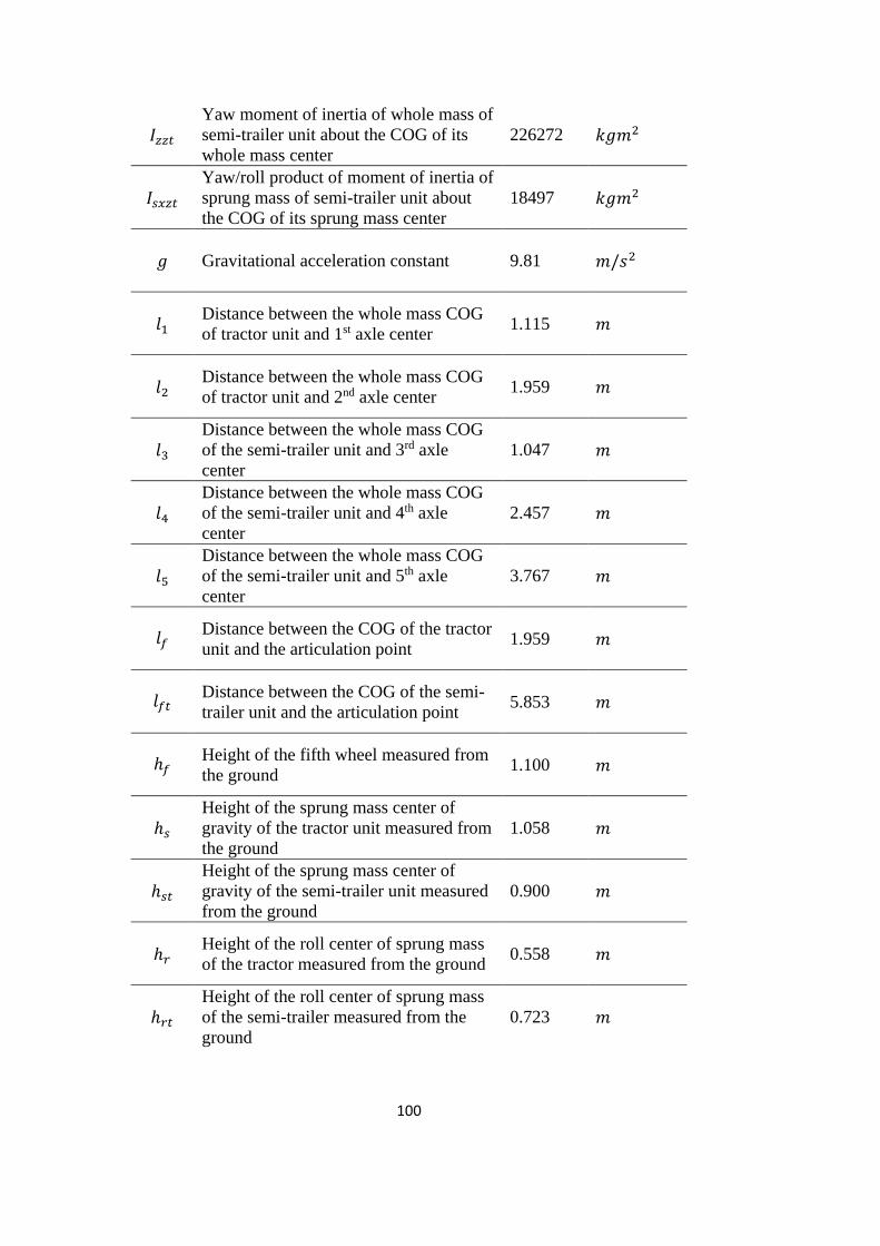
100
𝐼𝑧𝑧𝑡 Yaw moment of inertia of whole mass of
semi-trailer unit about the COG of its
whole mass center
226272 𝑘𝑔𝑚2
𝐼𝑠𝑥𝑧𝑡 Yaw/roll product of moment of inertia of
sprung mass of semi-trailer unit about
the COG of its sprung mass center
18497 𝑘𝑔𝑚2
𝑔 Gravitational acceleration constant 9.81 𝑚/𝑠2
𝑙1 Distance between the whole mass COG
of tractor unit and 1st axle center 1.115 𝑚
𝑙2 Distance between the whole mass COG
of tractor unit and 2nd axle center 1.959 𝑚
𝑙3
Distance between the whole mass COG
of the semi-trailer unit and 3rd axle
center
1.047 𝑚
𝑙4
Distance between the whole mass COG
of the semi-trailer unit and 4th axle
center
2.457 𝑚
𝑙5
Distance between the whole mass COG
of the semi-trailer unit and 5th axle
center
3.767 𝑚
𝑙𝑓 Distance between the COG of the tractor
unit and the articulation point 1.959 𝑚
𝑙𝑓𝑡 Distance between the COG of the semi-
trailer unit and the articulation point 5.853 𝑚
ℎ𝑓 Height of the fifth wheel measured from
the ground 1.100 𝑚
ℎ𝑠 Height of the sprung mass center of
gravity of the tractor unit measured from
the ground
1.058 𝑚
ℎ𝑠𝑡 Height of the sprung mass center of
gravity of the semi-trailer unit measured
from the ground
0.900 𝑚
ℎ𝑟 Height of the roll center of sprung mass
of the tractor measured from the ground 0.558 𝑚
ℎ𝑟𝑡 Height of the roll center of sprung mass
of the semi-trailer measured from the
ground
0.723 𝑚

101
ℎ∗ Difference in height of roll center of
sprung mass of the tractor unit and its
sprung mass COG
0.500 𝑚
ℎ𝑡∗
Difference in height of roll center of
sprung mass of the semi-trailer unit and
its sprung mass COG
0.177 𝑚
ℎ𝑓𝑟 Difference in height of roll center of
sprung mass of the tractor unit and the
height of fifth wheel
0.542 𝑚
ℎ𝑓𝑟𝑡 Difference in height of roll center of
sprung mass of the semi-trailer unit and
the height of fifth wheel
0.377 𝑚
∑𝐾𝜙 Total roll stiffness of suspensions and
tires of the tractor unit 1948060 𝑁𝑚/𝑟𝑎𝑑
∑𝐾𝜙𝑡 Total roll stiffness of suspensions and
tires of the semi-trailer unit 515660 𝑁𝑚/𝑟𝑎𝑑
∑𝐾12 Total roll stiffness of coupling point
between tractor and semi-trailer 114590 𝑁𝑚/𝑟𝑎𝑑
∑𝐶𝜙 Total roll damping of suspensions and
tires of the tractor unit 320000 𝑁𝑚𝑠/𝑟𝑎𝑑
∑𝐶𝜙𝑡 Total roll damping of suspensions and
tires of the semi-trailer unit 270000 𝑁𝑚𝑠/𝑟𝑎𝑑
𝐶1 Total cornering stiffness of the tires on
the front axle of the tractor 277200 𝑁/𝑟𝑎𝑑
𝐶2 Total cornering stiffness of the tires on
the rear axle of the tractor 740280 𝑁/𝑟𝑎𝑑
𝐶3 Total cornering stiffness of the tires on
the front axle of the semi-trailer 882000 𝑁/𝑟𝑎𝑑
𝐶4 Total cornering stiffness of the tires on
the middle axle of the semi-trailer 882000 𝑁/𝑟𝑎𝑑
𝐶5 Total cornering stiffness of the tires on
the rear axle of the semi-trailer 882000 𝑁/𝑟𝑎𝑑

102
103
APPENDIX C
MATRICES FOR THE CONTROL STRATEGIES
In this section, the state space matrices related to each control strategy is provided in
a detailed way. Recall the linear time invariant (LTI) state space system given by
equation (A50) in Appendix A.
�̇� = 𝑨𝒙 + 𝑩𝜹 (𝐶1)
Implementation of active trailer steering on the vehicle model brings about the
necessity of the modification of the matrices identified in Appendix A. For each
control strategy, the matrices associated with the articulated vehicle model controlled
by ATS systems are provided in Appendix C. The control strategies proposed by other
researchers is adopted to the vehicle model so that a comparison of the approaches
could be applied.
Matrices Related To the AHV Controlled with Steer Ratio Principle (SR):
In the study, the steer ratio principle is stated as an ATS strategy described with the
equation (4.9) previously. Rewrite the equation as follows:
𝛿𝑠 = 𝜇 𝛿1 (𝐶2)
Written for the steer ratio principle, the equation (C1) become in the form of the
following equation.
�̇� = 𝑨𝒙 + 𝑩𝛿1 + 𝑩𝒖𝛿𝑠 (𝐶3)
where the matrices are constructed as
[𝐴]8𝑥8 = [𝐴𝑖]8𝑥8−1[𝐵𝑖]8𝑥8

104
[𝐵]8𝑥1 = [𝐴𝑖]8𝑥8−1[𝐶𝑖]8𝑥1
[𝐵𝑢]8𝑥1 = [𝐴𝑖]8𝑥8−1[𝐶𝑖𝑢]8𝑥1
The matrices [𝐴𝑖]8𝑥8 and [𝐵𝑖]8𝑥8 is the same as the previously mentioned matrices in
Appendix A. On the other hand, [𝐶𝑖]8𝑥1 and [𝐶𝑖𝑢]8𝑥1 is identified with the following
matrix elements. Note that the matrices have elements having the value of zero except
the provided ones.
𝐶𝑖(1,1) = −𝐶1
𝐶𝑖(2,1) = −𝐶1(l1 + 𝑙𝑓)
𝐶𝑖(3,1) = −𝐶1ℎ𝑓𝑟
𝐶𝑖𝑢(1,1) = 𝐶𝑡
𝐶𝑖𝑢(4,1) = −𝐶𝑡(𝑙𝑡 + 𝑙𝑓𝑡)
𝐶𝑖𝑢(5,1) = 𝐶𝑡ℎ𝑓𝑟𝑡
where the equivalent cornering stiffness of the semi-trailer 𝐶𝑡 and equivalent distance
on which the actively steered axle is put on the semi-trailer 𝑙𝑡 is provided below.
𝐶𝑡 = 𝐶3 + 𝐶4 + 𝐶5
𝑙𝑡 =𝑙3 + 𝑙4 + 𝑙5
3
Since the active steering angle directly related to the driver steering input, the matrices
turns out to be the equation (C4) as follows.
�̇� = 𝑨𝒙 + 𝑩𝑺𝑹𝛿1 (𝐶4)
where the driver input matrix changed as 𝑩𝑺𝑹 = 𝑩+ 𝜇𝑩𝒖
Matrices Related To the AHV Controlled with Active Command Steering (ACS):
Command steering based active trailer steering is identified in the previous section,
having the following relation given by equation (C5):

105
𝛿𝑠 = 𝛽 𝜓𝑠 (𝐶5)
The form given in equation (C3) is valid for that ATS strategy, too. However, the
matrix associated with the active steering input is replaced as in the following
equation:
�̇� = 𝑨𝒙 + 𝑩𝛿1 + 𝑩𝑨𝑪𝑺𝜓𝑠 (𝐶6)
where the matrix associated with the command steering based active input is expressed
as 𝑩𝑨𝑪𝑺 = 𝛽𝑩𝒖. In this relation, the value of 𝛽 is determined as
𝛽 =𝑙𝑡
𝑙𝑡 + 𝑙𝑓𝑡
In this control strategy, the quadratic performance index is based on the minimization
of the states of the vehicle.
Matrices Related To the AHV Controlled with the Virtual Driver Steering
Controller (VD):
For the implementation of virtual driver steering controller (VD), recall the previously
mentioned states of the system.
𝒙𝑽𝑫 = [𝒙 𝑦𝑒 𝑦5𝑡ℎ 𝑦5𝑡ℎ𝛥 … 𝑦5𝑡ℎ𝑚𝛥]𝑇 (𝐶7)
where the first terms refers to the 8 original system states provided in Appendix A.
The other terms corresponds to the position of the rearmost point of the semi-trailer,
position of the fifth wheel and the time delayed positions of the fifth wheel,
respectively.
The additional differential equations are written as follows:
�̇�𝑒(𝑡) = 𝑣𝑡(𝑡) − 𝑙5𝑟𝑡(𝑡) (𝐶8)
�̇�5𝑡ℎ(𝑡) = 𝑣(𝑡) − 𝑙𝑓𝑟(𝑡) (𝐶9)
�̇�5𝑡ℎ𝑖(𝑡 − 𝑖𝛥) =1
𝛥[𝑦5𝑡ℎ(𝑡 − (𝑖 − 1)𝛥) − 𝑦5𝑡ℎ(𝑡 − 𝑖𝛥)] (𝐶10)
where 𝑖 = 1,2,3… ,𝑚 and 𝛥 = (𝑙𝑓𝑡 + 𝑙5)/𝑈.

106
The resultant matrices for the implementation of virtual driver steering controller are
expressed in the form of equation (C11):
{
�̇��̇�𝑒�̇�5𝑡ℎ�̇�5𝑡ℎ𝛥⋮
�̇�5𝑡ℎ𝑚𝛥}
= [[𝐴]8𝑥8 [0]8𝑥(𝑚)
[𝑇](𝑚+2)𝑥8 [𝐼](𝑚+2)𝑥(𝑚)]
{
𝒙𝑦𝑒𝑦5𝑡ℎ𝑦5𝑡ℎ𝛥⋮
𝑦5𝑡ℎ𝑚𝛥}
+ [[𝐵]8𝑥1
[0](𝑚+2)𝑥1] 𝛿1
+ [[𝐵𝑢]8𝑥1[0](𝑚+2)𝑥1
] 𝛿𝑠 (𝐶11)
where
[𝑇](𝑚+2)𝑥8 =
[ 0 1 0 −𝑙5 0 0 0 01 0 −𝑙𝑓 0 0 0 0 0
0 0 0 0 0 0 0 0⋮ ⋮ ⋮ ⋮ ⋮ ⋮ ⋮ ⋮0 0 0 0 0 0 0 0]
[𝐼](𝑚+2)𝑥(𝑚) =
[ 1/ 𝛥 −1/ 𝛥 0 0 0 00 1/ 𝛥 −1/ 𝛥 0 0 00 0 1/ 𝛥 −1/ 𝛥 0 0⋮ ⋱ ⋱ ⋱ ⋱ ⋮0 0 0 0 1/ 𝛥 −1/ 𝛥]
The quadratic performance index used in the LQR aims to minimize the lateral position
error between the lead point and the follow point, as explained in Section 4.
Matrices Related To the AHV Controlled with the Lateral Position Deviation
Preview Controller (LPDP):
For this control strategy, the modified states of the system are written as follows:
𝒙𝑳𝑷𝑫𝑷 = [𝒙 𝑦𝑟 𝑦𝑓 𝑦𝑓𝛥 … 𝑦𝑓𝑛𝛥]𝑇 (𝐶12)
where the additional states are the position of the centerline of the active semi-trailer
axle, position of the centerline of the tractor front axle, and its time delayed states,
respectively.
In addition to this, the relevant differential equations to be used with the original
equations of motions are given by equation (C13), (C14) and (C15):

107
�̇�𝑟(𝑡) = 𝑣𝑡(𝑡) − 𝑙3𝑟𝑡(𝑡) (𝐶13)
�̇�𝑓(𝑡) = 𝑣(𝑡) + 𝑙1𝑟(𝑡) (𝐶14)
�̇�𝑓(𝑡 − 𝑗𝛥) =1
𝛥[𝑦𝑓(𝑡 − (𝑗 − 1)𝛥) − 𝑦𝑓(𝑡 − 𝑗𝛥)] (𝐶15)
where 𝑗 = 1,2,3… , 𝑛 and 𝛥 = (𝑙1 + 𝑙𝑓 + 𝑙𝑓𝑡 + 𝑙𝑡)/𝑈.
As a result, the final form of the state-space matrices for the LPDP controller become
as follows:
{
�̇��̇�𝑟�̇�𝑓�̇�𝑓𝛥⋮
�̇�𝑓𝑛𝛥}
= [[𝐴]8𝑥8 [0]8𝑥(𝑛)
[𝑇](𝑛+2)𝑥8 [𝐼](𝑛+2)𝑥(𝑛)]
{
𝒙𝑦𝑟𝑦𝑓𝑦𝑓𝛥⋮
𝑦5𝑓𝑛𝛥}
+ [[𝐵]8𝑥1
[0](𝑛+2)𝑥1] 𝛿1
+ [[𝐵𝑢]8𝑥1[0](𝑛+2)𝑥1
] 𝛿𝑠 (𝐶16)
where
[𝑇](𝑛+2)𝑥8 =
[ 0 1 0 −𝑙3 0 0 0 01 0 𝑙1 0 0 0 0 00 0 0 0 0 0 0 0⋮ ⋮ ⋮ ⋮ ⋮ ⋮ ⋮ ⋮0 0 0 0 0 0 0 0]
[𝐼](𝑛+2)𝑥(𝑛) =
[ 1/ 𝛥 −1/ 𝛥 0 0 0 00 1/ 𝛥 −1/ 𝛥 0 0 00 0 1/ 𝛥 −1/ 𝛥 0 0⋮ ⋱ ⋱ ⋱ ⋱ ⋮0 0 0 0 1/ 𝛥 −1/ 𝛥]
For LPDP controller, the quadratic performance index used in the LQR try to minimize
the lateral position error between the position of tractor front axle centerline and active
semi-trailer axle centerline.
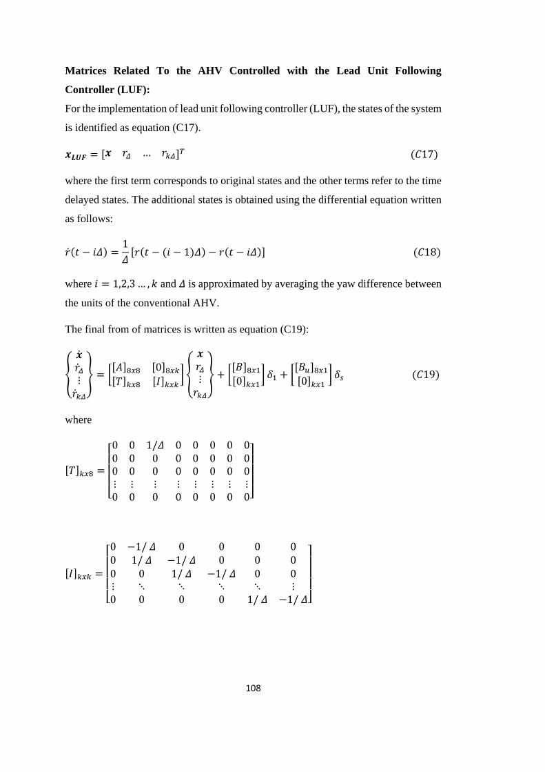
108
Matrices Related To the AHV Controlled with the Lead Unit Following
Controller (LUF):
For the implementation of lead unit following controller (LUF), the states of the system
is identified as equation (C17).
𝒙𝑳𝑼𝑭 = [𝒙 𝑟𝛥 … 𝑟𝑘𝛥]𝑇 (𝐶17)
where the first term corresponds to original states and the other terms refer to the time
delayed states. The additional states is obtained using the differential equation written
as follows:
�̇�(𝑡 − 𝑖𝛥) =1
𝛥[𝑟(𝑡 − (𝑖 − 1)𝛥) − 𝑟(𝑡 − 𝑖𝛥)] (𝐶18)
where 𝑖 = 1,2,3… , 𝑘 and 𝛥 is approximated by averaging the yaw difference between
the units of the conventional AHV.
The final from of matrices is written as equation (C19):
{
�̇��̇�𝛥⋮�̇�𝑘𝛥
} = [[𝐴]8𝑥8 [0]8𝑥𝑘[𝑇]𝑘𝑥8 [𝐼]𝑘𝑥𝑘
] {
𝒙𝑟𝛥⋮𝑟𝑘𝛥
} + [[𝐵]8𝑥1[0]𝑘𝑥1
] 𝛿1 + [[𝐵𝑢]8𝑥1[0]𝑘𝑥1
] 𝛿𝑠 (𝐶19)
where
[𝑇]𝑘𝑥8 =
[ 0 0 1/𝛥 0 0 0 0 00 0 0 0 0 0 0 00 0 0 0 0 0 0 0⋮ ⋮ ⋮ ⋮ ⋮ ⋮ ⋮ ⋮0 0 0 0 0 0 0 0]
[𝐼]𝑘𝑥𝑘 =
[ 0 −1/ 𝛥 0 0 0 00 1/ 𝛥 −1/ 𝛥 0 0 00 0 1/ 𝛥 −1/ 𝛥 0 0⋮ ⋱ ⋱ ⋱ ⋱ ⋮0 0 0 0 1/ 𝛥 −1/ 𝛥]

109
Matrices Related To the AHV Controlled with the Lateral Acceleration
Characteristic Following Controller (LACF):
In this study, LACF strategy is proposed for the ATS system. In order to accomplish
the lateral acceleration tracking, required states are identified as follows:
𝒙𝑳𝑨𝑪𝑭 = [𝒙 �̇� �̇�𝛥 … �̇�𝑙𝛥 𝑟𝛥 … 𝑟𝑘𝛥]𝑇 (𝐶20)
The lateral acceleration following necessitates to obtain the derivatives of the original
states. In the equation (C20), the first 2 terms stand for the original system states and
theirs derivatives as additional states. The other terms indicates the time delayed states
of the new system.
The differential equations given by (C21) and (C22) is used to derive the new state
space system for the LACF strategy.
�̈�(𝑡 − 𝑖𝛥) =1
𝛥[�̇�(𝑡 − (𝑖 − 1)𝛥) − �̇�(𝑡 − 𝑖𝛥)] (𝐶21)
where 𝑖 = 1,2,3… , 𝑙
�̇�(𝑡 − 𝑖𝛥) =1
𝛥[𝑟(𝑡 − (𝑖 − 1)𝛥) − 𝑟(𝑡 − 𝑖𝛥)] (𝐶22)
where 𝑖 = 1,2,3… , 𝑘
The resultant form is written as follows:
{
�̇��̈��̈�𝛥⋮�̈�𝑙𝛥�̇�𝛥⋮�̇�𝑘𝛥}
=
[ [𝐴]8𝑥8 [0]8𝑥8 [0]8𝑥𝑙 [0]8𝑥𝑘[0]8𝑥8 [𝐴]8𝑥8 [0]8𝑥𝑙 [0]8𝑥𝑘[0]𝑙𝑥8 [0]𝑙𝑥8 [𝐼]𝑙𝑥𝑙 [0]𝑙𝑥𝑘[𝑇]𝑘𝑥8 [0]𝑘𝑥8 [0]𝑘𝑥𝑙 [𝐼2]𝑘𝑥𝑘]
{
𝒙�̇��̇�𝛥⋮�̇�𝑙𝛥𝑟𝛥⋮𝑟5𝛥}
+ [
[𝐵]8𝑥1 [0]8𝑥1[0]8𝑥1 [𝐵]8𝑥1[0]𝑙𝑥1 [0]𝑙𝑥1[0]𝑘𝑥1 [0]𝑘𝑥1
] {𝛿1�̇�1}
+ [
[𝐵𝑢]8𝑥1 [0]8𝑥1[0]8𝑥1 [𝐵𝑢]8𝑥1[0]𝑙𝑥1 [0]𝑙𝑥1[0]𝑘𝑥1 [0]𝑘𝑥1
] {𝛿𝑠𝛿�̇�} (𝐶23)
where

110
[𝑇]𝑘𝑥8 =
[ 0 0 1/ 𝛥 0 0 0 0 00 0 0 0 0 0 0 00 0 0 0 0 0 0 0⋮ ⋮ ⋮ ⋮ ⋮ ⋮ ⋮ ⋮0 0 0 0 0 0 0 0]
[𝐼]𝑙𝑥𝑙 =
[ 1/ 𝛥 −1/ 𝛥 0 0 0 00 1/ 𝛥 −1/ 𝛥 0 0 00 0 1/ 𝛥 −1/ 𝛥 0 0⋮ ⋱ ⋱ ⋱ ⋱ ⋮0 0 0 0 1/ 𝛥 −1/ 𝛥]
[𝐼2]𝑘𝑥𝑘 =
[ 0 −1/ 𝛥 0 0 0 00 1/ 𝛥 −1/ 𝛥 0 0 00 0 1/ 𝛥 −1/ 𝛥 0 0⋮ ⋱ ⋱ ⋱ ⋱ ⋮0 0 0 0 1/ 𝛥 −1/ 𝛥]
In this case, there are two weighting factors associated with the quadratic performance
index explained in Section 4.

111
APPENDIX D
WEIGHT FACTOR DETERMINATION
In this section, the weighting factors associated with each control strategy for all the
test conditions are identified. For a quadratic performance index defined in the form
of Equation D1, the 𝑄 and 𝑅 matrices are the corresponding weighting factors of states
and control variables of the system, respectively.
𝐽 = ∫ (𝑥𝑇𝑄𝑥 + 𝑢𝑇𝑅𝑢)∞
0
𝑑𝑡 (𝐷1)
The given quadratic performance index can be rewritten as follows:
𝐽 = ∫ 𝜌1[𝑒(𝑡)]2
∞
0
+ 𝜌2[𝛿𝑠(𝑡)]2 𝑑𝑡 (𝐷2)
In that case, the cost function given by Equation D2 aims to minimize the defined error
𝑒(𝑡) with the use of the active steering control input 𝛿𝑠(𝑡). Also, corresponding
weighting factors for the error and control input are identified as 𝜌1 and 𝜌2,
respectively.
For the implementation of SR principle, Linear Quadratic Regulator technique is not
valid for the control strategy. Thus, any weighting adjustment associated with the ATS
strategy is not applicable in that case.
In case of ACS control strategy, the performance index given by Equation D1 is used
for the minimization of equally important state variables of the system. As a result, the
𝑄 matrix associated with that control strategy is described as an identity matrix. For

112
each test conditions, following procedure is followed: The 𝑄 matrix is chosen as an
identity matrix as mentioned above. Since there is only one virtual steerable axle, the
weighting matrix 𝑅 of the control input is a scalar quantity. Keeping the weighting of
states as identity matrix, the relative importance of the control input is adjusted
accordingly so that the best performance measures are obtained for each test maneuver.
For the remaining control strategies, the quadratic performance index in the form given
by Equation D2 is applicable. The terms 𝜌1 and 𝜌2 are two different weighting factor
in the cost function. At the beginning, the value of either weighting factor can be fixed.
Afterwards, the other weighting factor may be adjusted by observing the behavior
while its value is changing. Finally, the optimum weighting factors that provide the
best performance measure at each test conditions are chosen. Note that different set of
weight factors is associated with each standard test maneuvers. In addition, for the
proposed control strategy, a similar trial-error procedure is used for the determination
of the weighting factors.
On the other hand, there are some limitations for the use of some weighting factors set.
In the study, the limitations are taken into consideration while determining the
weighting factors associated with all control strategies:
Any weight factor sets that lead to the response exceeding a maximum 4° slip
angles at the axles should not be chosen. Therefore, the assumption of linearity
in the cornering stiffness is satisfied.
A weight factor set should provide the response having maximum 0.35g peak
lateral acceleration at the vehicle units. Thus, the vehicle responses remain in
the reasonable range of the linear vehicle model.