ARTICLE IN PRESS

0098-3004/$ - se

doi:10.1016/j.ca

$Code availa

index.htm

E-mail addr

Computers & Geosciences 34 (2008) 1263–1283

www.elsevier.com/locate/cageo

Modeling a dynamically varying mixed sediment bed witherosion, deposition, bioturbation, consolidation, and armoring$

Lawrence P. Sanford

Horn Point Laboratory, University of Maryland Center for Environmental Science, PO Box 775, Cambridge, MD 21613, USA

Received 15 August 2006

Abstract

Erosion and deposition of bottom sediments reflect a continual, dynamic adjustment between the fluid forces applied to

a sediment bed and the condition of the bed itself. Erosion of fine and mixed sediment beds depends on their composition,

their vertical structure, their disturbance/recovery history, and the biota that inhabit them. This paper presents a new one-

dimensional (1D), multi-layer sediment bed model for simulating erosion and deposition of fine and mixed sediments

subject to consolidation, armoring, and bioturbation. The distinguishing characteristics of this model are a greatly

simplified first-order relaxation treatment for consolidation, a mud erosion formulation that adapts to both Type I and II

erosion behavior and is based directly on observations, a continuous deposition formulation for mud that can mimic

exclusive erosion and deposition behavior, and straightforward inclusion of bioturbation effects. Very good agreement

with two laboratory data sets on consolidation effects is achieved by adjusting only the first-order consolidation rate rc.

Full model simulations of three idealized cases based on upper Chesapeake Bay, USA observations are presented. In the

mud only case, fluid stresses match mud critical stresses at maximum erosion. A consolidation lag results in higher

suspended sediment concentrations after erosional events. Erosion occurs only during accelerating currents and deposition

does not occur until just before slack water. In the mixed mud and sand case without bioturbation, distinct layers of high

and low sand content form and mud suspension is strongly limited by sand armoring. In the mixed mud and sand case with

bioturbation, suspended mud concentrations are greater than or equal to either of the other cases. Low surface critical

stresses are mixed down into the bed, constrained by the tendency to return towards equilibrium. Sand layers and the

potential for armoring of the bed develop briefly, but mix rapidly. This model offers a relatively simple and robust tool for

simulating the complex interactions that can affect muddy and mixed sediment bed erodibility.

r 2008 Elsevier Ltd. All rights reserved.

Keywords: Cohesive sediments; Consolidation; Bed armoring; Bioturbation; Sediment transport modeling; Critical stress; Sediment bed

model

e front matter r 2008 Elsevier Ltd. All rights reserved

geo.2008.02.011

ble from server at http://www.iamg.org/CGEditor/

ess: lsanford@hpl.umces.edu

1. Introduction

A ubiquitous challenge in predicting suspendedsediment concentrations and transport is specifyingthe rate at which a given sediment bed erodes (orresuspends, which is equivalent for present pur-poses). Erosion and its counterpart, deposition,

.

ARTICLE IN PRESS

Nomenclature

Dm difference in sediment mass betweensuccessive bed layers (kgm�2)

Dt model time step (d)a vertical gradient in mud critical stress

(Pam2 kg�1)b mass transfer coefficient for mud erosion

(md�1 Pa�1)dmi sediment mass in layer i (kgm�2)fs solids volume fraction, generalfseq equilibrium profile of mud solids volume

fractionfsN asymptotic mud solids volume fraction at

depthfs0 mud solids volume fraction at the surfacefsm solids volume fraction of mud matrixfsmin minimum solids volume fraction of newly

deposited mudfss solids volume fraction of sand matrixfstot total solids volume fraction of sand–mud

mixturego empirical resuspension coefficient for

sandk ¼ 0.4 von Karman’s constantr water density (kgm�3)rdry sediment dry density (kgm�3)rs sediment solids density (kgm�3)tb skin friction shear stress (Pa)tb0 skin friction at beginning of time step

(Pa)tc critical stress for erosion of mud (Pa)tceq equilibrium profile of mud critical stress

(Pa)tci mud critical stress at interface (Pa)tcmin minimal critical stress for deposited mud

flocs (Pa)tcminrelaxrelaxed value of the floc stress over time

Dt (Pa)tc0 mud critical stress at beginning of time

step (Pa)tcs critical stress for erosion of sand (Pa)

A time derivative of bottom stress (Pa d�1)Ab measure of bio-adhesionc depth decay scale for exponential poros-

ity profile in sediments (m�1)D deposition rate (kgm�2 d�1)Dbm, Dbz bio-diffusion coefficient (kg2m�4 d�1

or m2 d�1, respectively)E erosion rate (kgm�2 d�1)H Heaviside step functionM mud erosion rate parameter (kgm�2

d�1 Pa�1)NR correction factor for sand concentration

at a relative to water column averageR rouse numberS normalized excess stressVmm volume of the mud matrix (m3)Vms volume of the mud solids (m3)Vss volume of the sand solids (m3)a reference height for sand transport cal-

culations (m)cm1 average suspended mud concentration in

water column cell 1 (kgm�3)cs1 average suspended sand concentration in

water column cell 1 (kgm�3)dmi newly deposited mud floc mass (kgm�2)D50s median grain diameter of sand (m)dz thickness of newly deposited layer (m)fm mass fraction of mudfs mass fraction of sandm sediment bed mass coordinates (kgm�2)mmix amount of mass transferred by bioturba-

tion in both directions in time Dt

(kgm�2)rc consolidation rate (d�1)rs swelling rate (d�1)t time (d)u* shear velocity (md�1)wsm settling speed of suspended mud particles

(md�1)wss settling speed of suspended sand particles

(md�1)z sediment bed depth coordinates (m)

L.P. Sanford / Computers & Geosciences 34 (2008) 1263–12831264

reflect a continual, dynamic adjustment between thefluid forces applied to the sediment bed and thecondition of the bed itself. The most importantdescriptor of bed condition from this point of viewis erodibility, a combination of resistance to initialmotion (often expressed as a critical stress forerosion) and erosion rate once motion has begun

(often expressed as a function of the applied stressor the difference between applied stress and criticalstress).

Erosion of abiotic, non-cohesive sands and sandmixtures, whose stability depends primarily on theirexcess weight in water, is complex but reasonablywell understood and incorporated in models (Glenn

ARTICLE IN PRESSL.P. Sanford / Computers & Geosciences 34 (2008) 1263–1283 1265

and Grant, 1987; Harris and Wiberg, 2001; Li andAmos, 2001; Reed et al., 1999; Styles and Glenn,2005; Wiberg et al., 2002). The factors affectingerodibility of muds and sand–mud mixtures aremany and complex, however, and there is much lessagreement on how to model erosion of thesesediments. For purely fine, cohesive sediment beds,erodibility is a function of sediment grain size, watercontent, mineralogical composition, organics, ca-tion exchange capacity, and biological activity, aswell as the ionic composition, pH and temperatureof the water (Mehta, 1986; Paterson et al., 2000;Roberts et al., 1998; Tsai and Lick, 1987). Labora-tory remolded sediments tend to show little changein erodibility with depth into the bed (Roberts et al.,1998), but erodibility of deposited fine sedimentsoften decreases significantly with depth due toconsolidation, especially near the sediment surface(Mehta, 1988; Parchure and Mehta, 1985; Sanfordand Maa, 2001). When sediments are mixtures ofsands and muds, armoring of the bed surface bywinnowing of the fines also becomes an importantfactor limiting erodibility (Jones and Lick, 2001;Traykovski et al., 2004; Wiberg et al., 1994).Finally, mixtures of sand and mud appear to erodedifferently than either sediment type alone (Torfset al., 2001).

General recognition that fine sediment erodibilityis difficult to predict a priori has led to thedevelopment of a number of techniques to measureit directly, ranging from laboratory flume tests ofsediment samples from the field (Parchure andMehta, 1985; Tsai and Lick, 1987) to in situ testsusing either submersible flumes placed on thebottom (Amos et al., 1996; Gust and Morris,1989; Maa et al., 1998; Ravens and Gschwend,1999; Tolhurst et al., 2000) or carefully collectedcores (McNeil et al., 1996). These techniques oftenreveal large site-specific erodibility differences, asexpected, but repeated measures at the same sitealso reveal large temporal variability due to changesin sediment texture and biological activity (Maa andLee, 1994; Stevens et al., 2007). Laboratory(Parchure and Mehta, 1985; Tsai and Lick, 1987)and field (Droppo and Amos, 2001) studies havealso shown decreases in fine sediment erodibilityover time during consolidation, and increases inerodibility due to wave disturbance (Maa andMehta, 1987; Mehta, 1988).

It is apparent, then, that erosion of fine andmixed sediment beds depends not only on theircomposition, but also on their vertical structure,

their disturbance/recovery history, and the biotathat inhabit them. There are, at the present time,few if any models that explicitly incorporate thesefactors into a dynamically varying framework forpredicting changes in sediment erodibility. Thispaper describes an attempt at developing such amodel. A multi-layer bed model is formulated andtested to describe erosion and deposition of fine andmixed sediments subject to consolidation, armoring,and bioturbation. The distinguishing characteristicsof this model are a greatly simplified first-orderrelaxation treatment for consolidation, adoption ofa mud erosion formulation that adapts to both TypeI and II erosion behavior and is based directly onobservations, adoption of a continuous depositionformulation for mud that mimics exclusive erosionand deposition behavior, and straightforward in-clusion of bioturbation effects. The model isintended for situations in which surface erosion ofrelatively unconsolidated muddy and mixed sedi-ments is of primary interest.

2. Model development

2.1. Model structure

The sediment bed model was developed usingMATLABTM and it is coded in MATLABTM m-files. There are several different versions of the bedmodel presented here for different purposes, but allhave a number of things in common. They are allone-dimensional (1-D) vertical, time-dependent-layered bed models with piecewise continuousprofiles of the critical stress for erosion tc (Pa) orthe solids volume fraction fs, and layer-averagedvalues of the sand mass fraction fs, if necessary(Fig. 1). They all use sediment bed mass m (kgm�2)as the independent variable instead of depth,primarily because bed mass does not change duringconsolidation, whereas depth into the bed doeschange. All measure time in days, in keeping withtypical time scales for erosion, deposition, consoli-dation, and bioturbation. The values of tc or fs aredefined at the top of each layer, and are consideredto change linearly across each layer. Some of themodel versions are defined only for muds, but mostconsider a two-component mixture of non-cohesivesand and cohesive mud. Erosion and depositiononly occur between the water column and theuppermost (interface) bed level. The location of theinterface layer moves through the bed layer array toaccommodate excess erosion or deposition, as

ARTICLE IN PRESS

Fig. 1. Schematic representation of bed model structure. Left

column shows layer structure and variables as initialized; total

number of layers, critical stress profile, sand fraction, and mass of

each layer must be specified, as well as initial position of interface.

Right column shows layer structure and variables during a model

run. Interface layer occupies some fraction of its initial thickness

here. All erosion and deposition occur with interface layer, and a

separate variable keeps track of interface location. All other layer

thicknesses are as initialized, but critical stresses and sand

contents are variable. Bed mass is measured down from interface.

L.P. Sanford / Computers & Geosciences 34 (2008) 1263–12831266

needed. Mixing is allowed between bed layers, butonly when a mass transfer threshold is exceeded, inorder to minimize numerical dispersion. A largebuffer layer is defined at the bottom of the array toabsorb and dampen fluctuations that reach thebottom. Buffer layer properties may be mixed backup into the active sediment layers, but sediment maynot be eroded from or deposited to the buffer layer.In this paper, the model is solved explicitly with verysmall time intervals and very thin bed layers so as tobetter illustrate its structure and behavior. Furtherdetails are provided below.

2.2. Consolidation algorithm

A key assumption is that the effects of consolida-tion can be approximated as a first-order relaxation(exponential approach) to an empirically definedequilibrium state. There is, in fact, no apparentphysical reason that this should be so. Theequations governing self-weight consolidation of amud slurry are complex and inherently nonlinear(Toorman, 1996; Toorman and Berlamont, 1993;Winterwerp and Van Kesteren, 2004), and cannotbe transformed into the form of a first-order ODE

admitting to an exponential solution. However, ithas been known for some time that the meandensity of consolidating muddy beds approachesits final value in an approximately exponentialmanner (Hayter, 1986). Considering this fact andthe mathematical simplicity of a first-order relaxa-tion, the technique was adopted on an empirical,trial basis. Interestingly, Miller and Dean (2004)recently described a very similar approach formodeling the complex problem of shoreline change,in which present shoreline position is always tend-ing towards an equilibrium shoreline positionthat itself varies as a function of the nearshoreenvironment.

In a sense, the empiricism of the relaxationtowards equilibrium approach allows more freedomin its application, such that it is applied here toboth the increase in solids volume concentration(fs) and the increase in critical stress for erosion(tc) that accompany consolidation of a depositedcohesive sediment. It also does not require distin-guishing between the different phases of consolida-tion (Toorman and Berlamont, 1993), though itclearly would not be valid for segregation ofdifferent sediment classes by differential settling(Torfs et al., 1996) when the deposit is verywatery. Finally, it can equally well be applied todecreases in tc and fs that might occur duringswelling (albeit at a much slower rate), whenpreviously consolidated sediments are exposed tothe water column by erosion (Winterwerp and VanKesteren, 2004).

Equilibrium tc and fs profiles are defined asprimary functions of bed mass m and secondaryfunctions of other parameters:

ðtceq;fseqÞ ¼ functionðm; f s;Ab;S; . . .Þ (1)

where fs is the mass fraction of sand, Ab the measureof bio-adhesion, S the salinity, etc. The secondarydependencies listed after the semi-colon are includedin Eq. (1) for generality, but in the presentdevelopment the profiles are assumed to dependon m alone. The equilibrium profiles describe thestate of the sediment bed after long times with nodisturbance, such as might occur in a laboratorysettling column after many days. Here, it is assumedthat the equilibrium profiles are known, eitherthrough field experiments, laboratory experiments,or rigorous application of a consolidation model.Then at any point in time t and bed mass positionm the instantaneous value of the property ofinterest is assumed to approach equilibrium in a

ARTICLE IN PRESSL.P. Sanford / Computers & Geosciences 34 (2008) 1263–1283 1267

first-order sense

qtc

qt¼ rcðtceq � tcÞHðtceq � tcÞ

� rsðtceq � tcÞHðtc � tceqÞ

qfs

qt¼ rcðfseq � fsÞHðfseq � fsÞ

� rsðfseq � fsÞHðfs � fseqÞ (2)

where H is the Heaviside step function, defined suchthat H ¼ 1 when its argument is X0 and H ¼ 0otherwise. In Eq. (2), rc (d

�1) is the first-order con-solidation rate and rs (d

�1) is the first-order swellingrate, which is much smaller than rc; both rates arealso determined empirically or during model cali-bration. It is important to note that the equilibriumprofile is defined relative to the instantaneoussediment–water interface, so it moves down/upduring erosion/deposition, respectively. The use ofa bed mass coordinate rather than a depthcoordinate prevents the equilibrium profile frommoving down/up during consolidation/swelling.

Consolidation of mixed sediments is complex andsomewhat different from consolidation of puremuds. Torfs et al. (1996) carried out consolidationexperiments on mud–sand mixtures, and found thatthe presence of even a small amount of sand speedsup consolidation and results in a denser consoli-dated bed, as long as the initial mud density issufficient to prevent the sand from simply sinkingthrough and forming a separate deposit at thebottom. Some of the differences they describe maybe resolved by considering that the total bulkdensity of an unconsolidated mud is increasedsignificantly by the addition of sand. Consider alayer of a sand–mud mixture in which the sand(with mass dms) is suspended in a mud matrix (withmud mass dmm) such that the sand particles do notform a self-supporting structure. The total volumeof the mud matrix is V mm ¼ dmm=rsfsm, where fsm

is the solids volume fraction of the mud matrixalone. The total volume of the mud solids is V ms ¼

dmm=rs and the total volume of the sand solids isV ss ¼ dms=rs, and it is assumed for simplicity thatrs is the same for both sand and mud. Then the totalvolume of the mixture is Vmm+Vss and the totalsolids volume fraction of the mixture is

fstot ¼V ms þ Vss

Vmm þ Vss

¼1

f s þ ð1� f s=fsmÞ(3)

where f s ¼ dms=ðdmm þ dmsÞ. The situation is dif-ferent when the sand fraction is high enough to

form a self-supporting matrix. In this case, the mudis contained in the interstices between the sandparticles, and it may be shown that

fstot ¼fss

f s

¼0:55

f s

(4)

(Winterwerp and Van Kesteren, 2004). In Eq. (4),the solids volume fraction of the sand matrix (fss)has been set equal to a typical constant value of 0.55for simplicity.

For present purposes fstot is taken as theminimum value of Eqs. (3) and (4). At a constantvalue of fsm, as fs increases fstot first increases, thenreaches a maximum value between fs ¼ 0.8–0.97,then decreases to its pure sand value of 0.55 atfs ¼ 1. The total bulk density of the sedimentchanges in direct proportion to fstot. Using thisformulation accounts for the greater densities ofconsolidating mud–sand mixtures compared withpure muds, but it does not account for faster ratesof consolidation; i.e., rc is not a function of fs in thepresent model. There is, in concept, no reason thatthis change could not be implemented in the future.

Changes in rdry ¼ rsfstot affect most of the modelcases presented here only through erosion ratecalculations (see below), since the use of bed masscoordinates eliminates the need to know localdensity for calculating position in the bed. Theexception is that almost all consolidation data arereported in elevation/depth coordinates; so local drydensity is needed to convert the model predictionsfrom bed mass coordinates to elevation coordinates(z) for comparison to data. This is done using therelationship dz ¼ dm=rdry and integrating from afixed reference point. Implementation of the presentbed model in terms of elevation coordinates wouldbe feasible using this same conversion.

2.3. Erosion formulations

Erosion and resuspension are considered to beidentical for present purposes, both signifyingtransfer of sediment mass from the interface layerto the water column. Erosion and deposition onlyoccur from/to the interface layer in the presentmodel, though other models simulate the influencesof bioturbation and bedload-induced mixingthrough non-local injection from deeper layers(Boudreau, 1997b).

Cohesive sediment (mud) erosion is calculatedaccording to a simple extension of Sanford and Maa(2001), which allows for both limited mud supply

ARTICLE IN PRESSL.P. Sanford / Computers & Geosciences 34 (2008) 1263–12831268

(Type 1) and unlimited mud supply (Type 2)erosion. Briefly, assume a linear threshold erosionlaw of the form

Em ¼M½tbðtÞ � tcðmÞ� (5)

where Em(t) is the mud erosion rate (kgm�2 d�1),M the erosion rate parameter (kgm�2 d�1 Pa�1)assumed to be locally constant, tb(t) the time-varying skin friction shear stress, and tc(m) thecritical stress profile assumed to be locally linear inm. Differentiating Eq. (5) with respect to time t andrearranging, a first-order differential equation forEm is derived as

dEm

dtþ aMEm ¼M

dtb

dt(6)

where a ¼ dtc/dm (Pam2 kg�1) is the derivative ofcritical stress with respect to bed mass. Assumingthat A ¼ dtb/dt is constant over a model time stepDt (d), then the solution of Eq. (6) averaged over Dt

is

Em ¼A

að1� bÞHðAÞ þ bMðtb0 � tc0Þ

� �Hðtb0 � tc0Þ

(7)

where

b ¼1� expð�aMDtÞ

aMDt(8)

is the erosion mode parameter (unitless), tb0 is theskin friction at the beginning of the time step, tc0 isthe mud critical stress at the sediment–water inter-face at the beginning of the time step,

M ¼ f mrdryb ¼ ð1� f sÞrdryb (9)

is the erosion rate parameter, and b is a masstransfer coefficient (md�1 Pa�1). If aMDt is verylarge, then b-0 and Em is controlled by the timerate of increase of skin friction (A) balanced againstthe mass rate of increase of critical stress into thebed (a); in other words, erosion only occurs duringperiods of increasing skin friction and is stronglyType I. If aMDt is very small, then b-1 and Em isproportional to the excess applied stress; this isstandard, linear Type II erosion. The profile of tc(m)is used to estimate a at each time step. b is assumedto be constant and is set empirically, allowing thevalue of M in each layer to change with fs and rdry.

Non-cohesive sediment (sand) erosion is calcu-lated following a slightly modified version of the

expression in Harris and Wiberg (2001)

Es ¼ wss

f srdrygoS

1þ goS(10)

where wss is the sand settling speed (md�1), go is anempirical resuspension coefficient, S ¼ ðtb �

tcsÞ=tcs �Hðtb � tcsÞ �Hð2:5� RÞ is the normal-ized excess stress, tcs is the critical stress for erosionof sand, R ¼ wss=ku� is the Rouse number, k ¼ 0.4is von Karman’s constant, and u� ¼

ffiffiffiffiffiffiffiffiffiffitb=r

pis the

shear velocity (md�1). The difference betweenEq. (10) and Harris and Wiberg (2001) is that fs

here denotes the mass fraction of sand in theinterface layer, while it represented the volumefraction in their paper.

While it is known that erosion of sand–mudmixtures differs from erosion of either componentalone (Torfs et al., 2001; Van Ledden, 2002), thesedifferences are not modeled here but are left forfuture work. There are two primary reasons forpostponing this issue. The first is that the erosionbehavior of sand–mud mixtures is still poorlyunderstood, and accordingly its parameterizationfor modeling is even less certain. The second is thatarmoring/winnowing effects during erosion ofsand–mud mixtures can be simulated withoutinvoking explicit interaction effects in the erosionterms, as long as the erosion rate of each componentis proportional to the fraction of that component inthe interface layer. This assures that the availablemass of the more erodible component is controlledby the remaining mass of the less erodible compo-nent in the interface layer, and it cannot berecharged until that layer is completely eroded andthe one beneath exposed, or until new material isdeposited. Separation of sand and mud erosion isadopted here as a simplified initial approach to beused until data shows that it cannot be supported.

When necessary, the erosion rates of sand andmud are reduced to prevent removal of more thanone bed layer in a single time step. As long as thetime step of the model is reasonably fast, the onlyartifact of this limitation is to temporarily slow therate of net erosion.

2.4. Deposition formulation

Another key aspect of the present model devel-opment is its treatment of mud deposition. Labora-tory measurements often seem to support exclusiveerosion and deposition (Einstein and Krone, 1962;Partheniades, 1986; Self et al., 1989; van Leussen

ARTICLE IN PRESSL.P. Sanford / Computers & Geosciences 34 (2008) 1263–1283 1269

and Winterwerp, 1990), while field data tend tosupport continuous deposition (Bedford et al., 1988;Kranck and Milligan, 1992; Schubel, 1968). Sanfordand Halka (1993) considered the matter in detail,concluding that continuous deposition seemed towork better for modeling full-scale field conditions,but that the reasons for the discrepancies betweenlaboratory and field behaviors remained unresolved.They furthermore demonstrated that the distinctionis not trivial, significantly affecting both themagnitude and phasing of suspended sedimentrelative to the applied forcing.

Recently, Winterwerp and Van Kesteren (2004),reexamined the original laboratory experimentsbehind the exclusive erosion and deposition idea(Einstein and Krone, 1962), and showed that theresults could be equally well explained by allowingfor continuous deposition but invoking a gradualstrengthening of the bed; i.e., a developing resis-tance to resuspension. In keeping with this idea, thepresent model allows for continuous deposition ofthe mud component. The mud deposition rate isexpressed as

Dm ¼ wsmcm1 (11)

where wsm is the settling speed of the suspended mudparticles (md�1) and cm1 the average suspendedmud concentration (kgm�3) in the lowest watercolumn model cell. If there is any net deposition(Dm– Em40), the deposited mud carries with it aminimal critical stress tcmin that decreases thecritical stress of the interface but immediately beginsconsolidating as well. This allows rapid resuspen-sion under only moderate forcing, but rapiddeposition and an increasing resistance to erosionwhen forcing is very low. This formulation mimicsexclusive erosion and deposition behavior undersome conditions, and continuous deposition beha-vior under others.

Sand deposition is calculated using Ds ¼ NRwsscs1,where NR is a correction factor for the vertical profileof suspended sand, wss (md�1) is the settling speed ofthe suspended sand particles, and cs1 is the averagesuspended sand concentration (kgm�3) in the lowestwater column model cell. The correction factor NR

is required because the sand erosion function inEq. (10) was derived assuming that sand erosion anddeposition rates balance each other at steady statewhen evaluated at reference height a ¼ 3� d50s,where d50s (m) is the median grain diameter of thesand (Harris and Wiberg, 2001). The value of theerosion parameter go in Eq. (10) generally decreases

with increasing reference height. Calculating thedeposition rate using the average concentration inthe lowest water column cell (effectively at a heightmuch greater than a) but calculating the erosion rateusing go at a would result in erosion greatly exceedingdeposition at steady state, which would violate theassumptions behind Eq. (10). Using a value of NR

based on typical conditions is a way to approxi-mately correct for this imbalance. NR is estimatedhere using a steady-state Rouse profile (e.g., vanRijn, 1993) that depends on wss and a typical value ofu* for the problem of interest.

When necessary, the deposition rates of both sandand mud are reduced to prevent the addition ofmore than one bed layer in a single time step, and toprevent depositing more material than is availablein the water column in a single time step. The onlyartifact of this limitation is to temporarily slow therate of net deposition.

2.5. Bed layer adjustments during erosion,

deposition, and mixing

Net deposition rate (D– E) to the interface layerfor both sediment components is calculated at theend of each time step and carried forward to thenext time step; note that net erosion is just negativenet deposition according to this convention. At thebeginning of the next time step, the net depositedsediment mass is added to the interface layer andsubtracted from the water column. This ensures thatthe total sediment mass summed over the watercolumn and sediment bed is conserved for both mudand sand. Any changes to the bed structure (tc, a, fs)due to net erosion, net deposition, consolidation, orsediment mixing are calculated. The critical stressfor erosion of mud varies in time and with depthinto the bed, but the critical stress for erosion ofsand is assumed to remain constant. Any changesto the water column structure (cm, cs) are alsocalculated, e.g., if there are multiple water columncells, which are not modeled here but are straight-forward to include. The new interface layer proper-ties and water column concentrations are used tocalculate erosion and deposition for the followingtime step.

When net erosion occurs, the interface mudcritical stress tci is adjusted by interpolating betweenits previous time step value and the previous timestep value of tci+1 (the mud critical stress at theboundary between the interface layer and the nextlayer down), based on the ratio of the total eroded

ARTICLE IN PRESSL.P. Sanford / Computers & Geosciences 34 (2008) 1263–12831270

mass to the total mass in the interface layer. Allvalues of tc in the bed are then relaxed towardsequilibrium. If the remaining mass in the interfacelayer is less than 10% of the original layer mass,then the remaining mass is added to the layer below,which is redefined as the new interface layer.Weighted averaging is used to calculate the newinterface layer mud and sand masses. The calculatedvalue of tci remains unchanged.

When net deposition occurs, the mud criticalstress profile in the interface layer may be thoughtof as a thin floc layer with constant critical stresstcmin on top of a layer with a linear profile of criticalstress. To return the interface layer to a single linearprofile of critical stress, the value of tci isrecalculated in order to preserve the mud mass-weighted average critical stress in the interface layer,but with a linear variation between tci and tci+1.This calculation is done after any adjustments ofmass and critical stress; i.e., the new floc criticalstress tcmin and the previous value of tci are bothrelaxed towards equilibrium before the calculation.Defining the relaxed value of the floc stress astcmin relax and the relaxed value of tci as tcirelax, thenew estimate of tci is given by

tci ¼ tcirelax �dmi

dmi

ðtcirelax þ tciþ1 � 2tcmin relaxÞ (12)

where dmi is the newly deposited floc mass and dmi

is the total amount of mud in the interface layer. Ifthe total mass in the interface layer exceeds 190% ofits initially established value, then the layer is splitinto two parts and the top 90+% of material isadded to the layer above, which is then redefined asthe interface layer. The adjusted value of tci remainsunchanged, but a new value of tci+1 is calculated byinterpolation.

Sediment bed mixing due to bioturbation ismodeled by assuming a constant biodiffusioncoefficient, Db (Boudreau, 1997a) but implementedin bed mass coordinates rather than depth coordi-nates (Officer and Lynch, 1989). Since Db is usuallyreported in a depth reference frame with units ofm2 d�1, it must be converted to a mass referenceframe using Dbm ¼ DbzðrsfstotÞ

2 (Officer and Lynch,1989), with units of kg2m�4 d�1. Rather thanallowing Dbm to vary with changing fstot, it issimply kept at a constant value here by using asingle representative value of fstot for the problemof interest.

Mixing is calculated in different ways for thelayer-averaged parameters and the piece-wise con-

tinuous parameters. In both cases, a vector of thedifference in mass between successive layers iscalculated and identified as Dm. A vector of masstransfer coefficients is then defined as Dm/Dm. Theamount of mass that would be transferred bybioturbation in both directions in time Dt ismmix ¼ DmDt=Dm; note that mmix,j is defined forthe boundary between layers j and j+1. For layer-averaged variables such as the mass of sandms, when mixing occurs the change in mass iscalculated as

Dms;j ¼ mmix;j�1ðf s;j�1 � f s;jÞ þmmix;jðf s;jþ1 � f s;jÞ

(13)

modified by dropping the first/second term on theright-hand side (RHS) for the top/bottom layers,respectively. For piecewise continuous variablessuch as the mud critical stress tc, first recall thatthe vector of the gradient in critical stress is definedas a. Then when mixing occurs the change in tc iscalculated as

Dtc;j ¼ mmix;j�1ðaj � aj�1Þ (14)

which is the numerical representation of

qtc ¼ Dbm

q2tc

qm2qt (15)

In order to minimize numerical dispersion byfrequent mixing of very small amounts of mass, themodel time step Dt in the above is replaced with thetime since the last mixing event and time is allowedto accumulate with no mixing until mmix for theboundary between the interface layer and the layerbelow is greater than some percentage of the mass inthe interface layer; 30% is used in the examplesshown here. A higher threshold percentage results invery little numerical dispersion but more pro-nounced changes in bed properties and erosionwhen mixing does occur, while a lower percentagegives smoother behavior but greater artificialdispersion of bed properties. When mixing occurs,it is calculated before any adjustments due toerosion, deposition, or consolidation.

At the end of each time step, all variables in thebed layers above the interface layer are zeroed andthe layers become inactive until they are repopu-lated by deposition.

2.6. The water column

In the cases presented here, the water column ismodeled as a well-mixed layer of depth 2m that

ARTICLE IN PRESSL.P. Sanford / Computers & Geosciences 34 (2008) 1263–1283 1271

gains and loses sediment only through erosion anddeposition across the sediment–water interface.Ignoring the changing vertical structure of watercolumn suspended sediment profiles results in someuncertainty in estimating the rate of deposition. Fortime-varying forcing, ignoring the phase lagsassociated with vertical diffusion of newly erodedmaterial and settling of suspended material alsoaffects the timing of deposition. However, forpresent purposes these effects are relatively minor.Resolution of the vertical structure of the watercolumn would be relatively straightforward, but it isnot done here to retain a central focus on thesediment bed structure and its dynamic behavior.

3. Example model calculations

3.1. Consolidation tests

Two simplified special versions of the model weredeveloped for comparison to data on consolidationeffects in muddy sediments. The first models theevolution of vertical profiles of sediment solidsvolume fraction and bulk density for a slurry placedinto a laboratory settling column. The secondmodels the evolution of profiles of critical stressfor a slurry placed into a laboratory annular flume.Both do not consider erosion, deposition, orsediment mixing, but do include a large number ofsediment layers for more accurate projections.

Bulk density profile predictions are comparedwith data reported by Toorman and Berlamont

Fig. 2. Comparisons between consolidation model predictions and da

data of Toorman and Berlamont (1993). Initial condition is represented

represented by thin line through triangular data points on right. Model p

through data points represented by squares and circles, respectively. Rig

data of Tsai and Lick (1987). Initial condition (at 1 d) is represented

equilibrium profile (at 7 d) is represented by thin line through triangular

line through circular data points.

(1993) in Fig. 2a. They reported on a laboratoryconsolidation experiment with ‘‘Doel Dock Mud’’in a 2m deep settling column. Bulk density may berelated to solids volume fraction by rb ¼ rsfstotþ

rð1� fstotÞ, where r is the density of water.The initial bulk density of the slurry was rb ¼

1050 kgm�3, corresponding to a solids volumefraction of fstot ¼ 0.03 assuming a solids densityof rs ¼ 2650 kgm�3. The slurry contained 3.5%sand, which apparently settled rapidly through themud and accumulated at the bottom of the column.Thus, the experiment was modeled here as a puremud starting with a uniform vertical profile withfstot ¼ 0.03 at time zero. An equilibrium profile wasobtained by fitting the exponential profile shapedescribed by Mulsow et al. (1998) (and used bymany others) to the observed profile at 14 d. Thegeneral profile shape is given by

fs ¼ f1 � ðf1 � fs0Þexpð�czÞ (16)

where fs0 is the solids volume fraction at the surfaceand fsN the asymptotic solids volume fractionat depth. The fitted profile with fs0 ¼ 0.036,fsN ¼ 0.076, and c ¼ 12m�1 is shown in Fig. 2a.It was converted to mass coordinates and used asinput to the consolidation model. Profiles at 0.11and 0.92 d were fit to the data by adjusting theconsolidation rate rc, yielding an optimal value ofrc ¼ 0.9 d�1. Predictions were converted back todepth coordinates for comparison to the data.

The agreement between the model predictionsand the data at 0.11 and 0.92 d is quite good in the

ta. Left panel: comparison between bulk density predictions and

by thin vertical line on left, while equilibrium profile (at 14.1 d) is

redictions at 0.11 and 0.92 d are represented by thick vertical lines

ht panel: comparison between critical stress profile predictions and

by thin line through data points represented by squares, while

data points. Model predicted profile at 2 d is represented by thick

ARTICLE IN PRESSL.P. Sanford / Computers & Geosciences 34 (2008) 1263–12831272

upper part of the density profile above the sand. Thesettling rate of the interface is also well predicted. Infact, these simple relaxation towards equilibriumpredictions are at least as good as the fullconsolidation model predictions described by Toor-man and Berlamont (1993), in the upper parts of theprofiles. The present model predictions and the datadiverge in the lower parts of the profiles because ofthe initial differential settling of sand through theslurry. The accumulation of sand at the bottom ofthe column caused a significant increase in the bulkdensity there, in accordance with Eq. (3). Thepresent model does not consider differential settlingof sand and mud within the sediment bed.

Critical stress profile predictions are comparedwith data reported by Tsai and Lick (1987). Theyconducted laboratory erosion experiments on mud-dy sediments collected from 20m depth in LongIsland Sound, NY. The sediments were screenedand stirred, then placed in an annular flume andthoroughly resuspended before being allowed tosettle and consolidate for different periods of time.In the erosion experiments, constant shear stresseswere applied to the sediment surface for intervals of1–2 h, then increased to a higher level for 1–2 h, etc.,up to a maximum stress of 1.2 Pa. At almost alllevels, sediment erosion stopped after approxi-mately 1

2h, which was interpreted as erosion of

all available sediment at that applied stress. Themass of sediment eroded at each applied stressduring experiments carried out after 1, 2, and 7 d ofconsolidation was reported, and these data areplotted in Fig. 2b.

For model comparison, the data at 7 d were takenas representative of the equilibrium profile of criticalstress vs. m. A power law fit to the data yielded

tceq ¼ 0:93m0:25; r2 ¼ 0:92 (17)

A similar profile fit to the data at 1 d ðtc ¼

0:49m0:26Þ was used to initialize the model. Thepredicted profile at 2 d was fit to the data byadjusting the consolidation rate rc, yielding anoptimal value of rc ¼ 0.9 d�1. Remarkably (andprobably coincidentally), this is the same consolida-tion rate as in the first comparison above. Again,the general fit to the shape of the critical stressprofile after 2 d is quite good (Fig. 2b). It is notablethat it was not necessary to invoke a depth or bedmass-dependent consolidation rate in either of thecomparisons presented here, although that would bepossible should it be required to fit another data set.

3.2. Full-scale model tests

This section illustrates application of the full-scalemodel with erosion, deposition, bioturbation, con-solidation, and armoring to three idealized testcases. The test cases are based loosely on observa-tions from upper Chesapeake Bay, USA. They areforced by tidally varying stress, modulated over twospring–neap cycles and punctuated by a 1.25-d highstress event. The same forcing and same sedimentproperties are used in all cases, starting with a puremud bed, adding a sand fraction, and addingsediment mixing due to bioturbation.

3.2.1. Observations from upper Chesapeake Bay

A bottom tripod and two taut-wire mooringswere deployed near 39116.10N, 76115.80W at adredged sediment disposal site in upper ChesapeakeBay, USA, from September 17–28, 1992. As part ofthe overall instrumentation package, an S4 currentmeter (InterOcean) was mounted on the tripod at1m above bottom (mab) and configured as a burst-sampling wave/tide/current gauge, and a Sea-Techtransmissometer was mounted at 3mab nearby.Turbidity from the transmissometer was calibratedto suspended sediment concentration using in situwater samples. The water depth at the tripod sitewas about 4.5m, and the bottom was nearly 100%mud removed from the adjacent shipping channelapproximately 10 months previous during main-tenance dredging operations.

Maximum tidal currents at 1mab were typicallybetween 0.4 and 0.5m s�1, and peak tidally re-suspended sediment concentrations were 0.005–0.025 kgm�3 above background levels in responseat the beginning of the deployment (Fig. 3). Threeshort episodes of winds and small waves punctuatedthe first 9 d of the deployment, but on September25–26 tropical storm ‘‘Danielle’’ passed directlyover the upper Bay with winds 4 15m s�1 blowingdirectly down the direction of longest fetch. Max-imum waves (from pressure records) were 0.75mhigh with approximately 3 s periods, which in 4.5mof water corresponded to maximum instantaneousnear-bottom velocities of about 0.20m s�1. Thepeak of the storm occurred approximately at thesame time as a strong ebb tide, such that sedimentsmobilized by the wave forcing were carried well upinto the water column with suspended sedimentconcentrations of approximately 0.150 kgm�3 at3mab. More interesting is the fact that tidal re-suspension after the storm had passed was markedly

ARTICLE IN PRESS

Stn 6, 1m

Stn 8, 3m

Stn 6, 1m

Howell Pt. Buoy

September 199217

Spe

ed (c

m/s

)

0102030405060

RM

S P

(mb)

02468

10

TSP

(mg/

l)

0

50

100

150

200

(Win

d S

peed

)2

050

100150200250

18 19 20 21 22 23 24 25 26 27 28 29

Fig. 3. Time-series observations of mud resuspension before, during and after a storm, from a site in upper Chesapeake Bay, MD, USA.

Top panel: wind speed squared from a nearby meteorological buoy. Second panel: root mean square pressure data from a burst-sampled

S4 current meter 1m above bottom (mab), approximately proportional to wave height. Third panel: total suspended sediment

concentration estimated from calibrated transmissometer measurements on a nearby mooring at 3mab. Bottom panel: 5min averaged

current speeds from same S4 current meter.

L.P. Sanford / Computers & Geosciences 34 (2008) 1263–1283 1273

greater than before the storm, while tidal forcingwas approximately the same as before the storm.Tidal resuspension levels of 0.05–0.1 kgm�3 abovebackground levels persisted for the remaining 3 dof the deployment. This appears to have beencaused by disturbance of the surface sedimentsduring the storm that made them more easilyerodible for some period following the storm. Therewas no evidence of large-scale delivery of newsediments associated with the storm that might havehad the same effect. These changes in erodibility dueto bottom sediment disturbance are among thedynamic behaviors that the present model seeks tomimic.

3.2.2. Full model test cases

The first of the three test cases is a 100% mud bedwith 25 bed layers 0.05 kgm�2 thick and a bottombuffer layer 3.75 kgm�2 thick. The equilibriumcritical stress profile is set equal to the average

Baltimore Harbor, MD, USA critical stress profilereported by Sanford and Maa (2001)

tceq ¼ 0:86ðmþ 0:0034Þ0:5 (18)

where the m ¼ 0 offset value has been adjustedslightly to give tceqð0Þ ¼ 0:05Pa (a more reasonableequilibrium value than the 0.01 minimum valuereported in their paper). A relationship between fsm

and tc was also reported, that was implied if M wasto satisfy Eq. (9); fsm was not directly measured atthe small vertical scales of the erosion tests. Thisrelationship is modified slightly to

fsm ¼ maxtc

9:3

� �0:93;fsmin

� �(19)

to ensure that fsmð0ÞXfsmin ¼ 0:03 in the presentmodel. The reported value of b ¼ 11.75md�1

Pa�1 ¼ 1.36� 10�4m s�1 Pa�1 is also used here.The water column is modeled as a 2m deep well-mixed box for simplicity; this is less than the 4.5m

ARTICLE IN PRESS

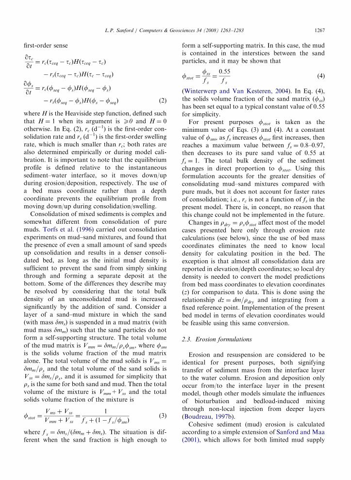
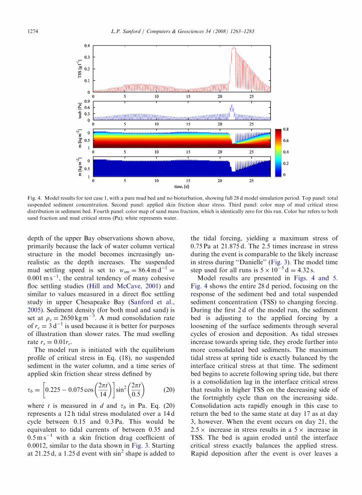
Fig. 4. Model results for test case 1, with a pure mud bed and no bioturbation, showing full 28 d model simulation period. Top panel: total

suspended sediment concentration. Second panel: applied skin friction shear stress. Third panel: color map of mud critical stress

distribution in sediment bed. Fourth panel: color map of sand mass fraction, which is identically zero for this run. Color bar refers to both

sand fraction and mud critical stress (Pa); white represents water.

L.P. Sanford / Computers & Geosciences 34 (2008) 1263–12831274

depth of the upper Bay observations shown above,primarily because the lack of water column verticalstructure in the model becomes increasingly un-realistic as the depth increases. The suspendedmud settling speed is set to wsm ¼ 86:4md�1 ¼0:001m s�1, the central tendency of many cohesivefloc settling studies (Hill and McCave, 2001) andsimilar to values measured in a direct floc settlingstudy in upper Chesapeake Bay (Sanford et al.,2005). Sediment density (for both mud and sand) isset at rs ¼ 2650 kgm�3. A mud consolidation rateof rc ¼ 3 d�1 is used because it is better for purposesof illustration than slower rates. The mud swellingrate rs ¼ 0.01rc.

The model run is initiated with the equilibriumprofile of critical stress in Eq. (18), no suspendedsediment in the water column, and a time series ofapplied skin friction shear stress defined by

tb ¼ 0:225� 0:075 cos2pt

14

� �sin2

2pt

0:5

(20)

where t is measured in d and tb in Pa. Eq. (20)represents a 12 h tidal stress modulated over a 14 dcycle between 0.15 and 0.3 Pa. This would beequivalent to tidal currents of between 0.35 and0.5m s�1 with a skin friction drag coefficient of0.0012, similar to the data shown in Fig. 3. Startingat 21.25 d, a 1.25 d event with sin2 shape is added to

the tidal forcing, yielding a maximum stress of0.75 Pa at 21.875 d. The 2.5 times increase in stressduring the event is comparable to the likely increasein stress during ‘‘Danielle’’ (Fig. 3). The model timestep used for all runs is 5� 10�5 d ¼ 4.32 s.

Model results are presented in Figs. 4 and 5.Fig. 4 shows the entire 28 d period, focusing on theresponse of the sediment bed and total suspendedsediment concentration (TSS) to changing forcing.During the first 2 d of the model run, the sedimentbed is adjusting to the applied forcing by aloosening of the surface sediments through severalcycles of erosion and deposition. As tidal stressesincrease towards spring tide, they erode further intomore consolidated bed sediments. The maximumtidal stress at spring tide is exactly balanced by theinterface critical stress at that time. The sedimentbed begins to accrete following spring tide, but thereis a consolidation lag in the interface critical stressthat results in higher TSS on the decreasing side ofthe fortnightly cycle than on the increasing side.Consolidation acts rapidly enough in this case toreturn the bed to the same state at day 17 as at day3, however. When the event occurs on day 21, the2.5� increase in stress results in a 5� increase inTSS. The bed is again eroded until the interfacecritical stress exactly balances the applied stress.Rapid deposition after the event is over leaves a

ARTICLE IN PRESS

Fig. 5. Detail of model results for test case 1, with a pure mud bed and no bioturbation, showing period of large event (left column) and a

single tidal cycle during recovery from event (right column). Top panels: total suspended sediment concentration. Second panels: net

deposition (deposition–erosion). Third panels: applied skin friction shear stress. Bottom panels: color map of mud critical stress

distribution in sediment bed.

L.P. Sanford / Computers & Geosciences 34 (2008) 1263–1283 1275

thick layer of easily eroded sediment, resulting inhigh levels of tidal resuspension that persist butgradually decay over the succeeding 6 d as the bedconsolidates. The modeled pattern of event responseis quite similar to the observations shown in Fig. 3;in fact, modeled TSS values are also similar toobserved values over the entire period if they arescaled by the relative depths of the water columns.

Fig. 5 shows detailed patterns of erosion anddeposition during the event and over a single tidalcycle 3 d after the event, in relation to forcing, TSS,and sediment bed response. Note that the predic-tions shown here represent net erosion and deposi-tion, which is almost always the small differencebetween much larger gross rates of erosion anddeposition because of our assumption of continuousdeposition (Eq. (11)). As stress increases at thebeginning of the event, the pre-event pattern ofalternating tidal erosion and deposition is sup-

planted for one tidal cycle by tidally pulsed erosiononly, followed by a tidal cycle with neither erosionnor deposition when bed erosion has reached itslimit but stresses are too high to allow net depo-sition, followed finally by massive deposition. Threedays after the event, large deposition near slackwater is almost, but not entirely, overcome by largeerosion after slack. Enough sediment consolidatesduring and after slack water to leave a small netdeposit behind on each cycle, which results ingradual build up of the bed over a period of severaldays. This is similar to the depositional processreported in the Hudson River turbidity maximumby Traykovski et al. (2004).

Focusing on a single tidal cycle in Fig. 2billustrates two important aspects of this model.First, erosion occurs only during acceleratingcurrents when the erodible sediment supply islimited (Maa and Kim, 2002; Sanford and Maa,

ARTICLE IN PRESS

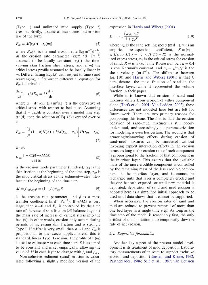
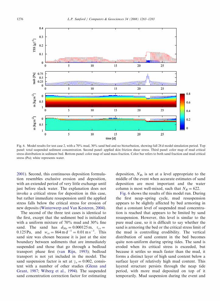
Fig. 6. Model results for test case 2, with a 70% mud, 30% sand bed and no bioturbation, showing full 28 d model simulation period. Top

panel: total suspended sediment concentration. Second panel: applied skin friction shear stress. Third panel: color map of mud critical

stress distribution in sediment bed. Bottom panel: color map of sand mass fraction. Color bar refers to both sand fraction and mud critical

stress (Pa); white represents water.

L.P. Sanford / Computers & Geosciences 34 (2008) 1263–12831276

2001). Second, this continuous deposition formula-tion resembles exclusive erosion and deposition,with an extended period of very little exchange untiljust before slack water. The explanation does notinvoke a critical stress for deposition in this case,but rather immediate resuspension until the appliedstress falls below the critical stress for erosion ofnew deposits (Winterwerp and Van Kesteren, 2004).

The second of the three test cases is identical tothe first, except that the sediment bed is initializedwith a uniform mixture of 70% mud and 30% finesand. The sand has d50s ¼ 0.000125m, tcs ¼

0.125 Pa, and wss ¼ 864md�1 ¼ 0.01m s�1. Thissand size was chosen because it is just at the sizeboundary between sediments that are immediatelysuspended and those that go through a bedloadtransport phase first (van Rijn, 1993); bedloadtransport is not yet included in the model. Thesand suspension factor is set at go ¼ 0.002, consis-tent with a number of other studies (Glenn andGrant, 1987; Wiberg et al., 1994). The suspendedsand concentration correction factor for estimating

deposition, NR, is set at a level appropriate to themiddle of the event when accurate estimates of sanddeposition are most important and the watercolumn is most well-mixed, such that NR ¼ 622.

Fig. 6 shows the results of this model run. Duringthe first neap–spring cycle, mud resuspensionappears to be slightly affected by bed armoring inthat a constant level of suspended mud concentra-tion is reached that appears to be limited by sandresuspension. However, this level is similar to thepure mud case, so it is difficult to say whether thesand is armoring the bed or the critical stress limit ofthe mud is controlling erodibility. The verticaldistribution of sand content in the bed becomesquite non-uniform during spring tides. The sand iseroded when its critical stress is exceeded, butbecause it settles so much faster than the mud, itforms a distinct layer of high sand content below asurface layer of relatively high mud content. Thislayered structure persists through the neap tideperiod, with more mud deposited on top of ittemporarily. Mud suspension during the event and

ARTICLE IN PRESS

Fig. 7. Model results for test case 3, with a 70% mud, 30% sand bed and moderate bioturbation, showing full 28 d model simulation

period. Top panel: total suspended sediment concentration. Second panel: applied skin friction shear stress. Third panel: color map of mud

critical stress distribution in sediment bed. Bottom panel: color map of sand mass fraction. Color bar refers to both sand fraction and mud

critical stress (Pa); white represents water.

L.P. Sanford / Computers & Geosciences 34 (2008) 1263–1283 1277

afterwards is very limited by sand armoring, partlybecause the mud erosion rate is limited by the sanderosion rate (not shown), but also because the rapidsettling velocity and deposition rate of the sandagain create a thick layer of high sand contentthrough which even the high event stresses cannotpenetrate. The levels of sand suspension at the peakof the event are consistent with expectation for anequilibrium Rouse profile, but they are too low toallow removal of the entire sand layer. This layerpersists after the event and a consolidating mud bedbegins to develop on top of it. The mud criticalstress during the event is much too low to controlbed erodibility, providing a clear indication ofarmoring.

The last of the three test cases is identical to thesecond case, except that bed mixing by bioturbationis simulated by setting Db ¼ 10 cm2 year�1 ¼ 2.73�10�6m2 d�1 ¼ 3.16� 10�11m2 s�1, which translatesto Dm ¼ 0.108 kg2m�4 d�1 in bed mass coordinates.This is a moderate level of bioturbation in coastalenvironments (Boudreau, 1997a).

Fig. 7 shows the results of this last model run, forcomparison to Figs. 4 and 6. Bioturbation-inducedsediment mixing has a huge effect on all aspects ofthe predictions. Suspended mud concentrations are3 times higher than either of the other cases duringthe first spring tide period, and equal to the puremud case during the event. This is becausebioturbation mixes both the critical stress profileand the sand content distribution. Sand layers andthe potential for armoring of the bed developbriefly, but are rapidly mixed away. The lowercritical stresses of the interface are mixed muchdeeper into the bed, although they are always beingpulled back towards the equilibrium profile. Lack ofarmoring and downward mixing of low criticalstress lead to the surprisingly large response duringspring tides. Note that the interface critical stress atpeak spring tides is still exactly equal to the appliedstress, however; the same is true of the event period.These results are consistent with published resultsindicating that bioturbation tends to increasesediment erodibility in both experimental (Tsai

ARTICLE IN PRESSL.P. Sanford / Computers & Geosciences 34 (2008) 1263–12831278

and Lick, 1987; Willows et al., 1998) and natural(Roast et al., 2004; Widdows et al., 1998, 2004)settings.

One of the more intriguing aspects of this case isthat bioturbation spreads fluctuations in sandfraction downward, rather than spreading themequally upward and downward. This is especiallynotable following the two major erosion periodsaround days 7 and 21 and the two major depositionperiods afterwards, but it is also true during eachtidal cycle. This downward mixing occurs for tworeasons. First, the surface is the source of the sandcontent fluctuations, which can only move down-ward and away from the surface. Second, thebottom buffer layer is absorbing these changes with-out reflecting them because of its large total mass.

4. Discussion

The model presented here offers intriguingpossibilities for simulating interactions betweensuspended sediments in the water column anddeposited sediments in the surface layers of thesediments, as mediated through erosion and deposi-tion. It is not intended to model all conceivablesituations, however. The model is biased towardsmuddy sediments that may contain a significantsand fraction, but for which cohesive behaviordominates. It is also biased towards low-moderateenergy environments where surface erosion andunhindered particle deposition dominate; i.e., wherefluid mud processes (Mehta and Srinivas, 1993;Trowbridge and Kineke, 1994; Wright et al., 2001)are not important.

There are a number of ways in which the modelmight be improved and expanded. The mostimportant of these is in its treatment of the sandfraction. The fine sand used in the examplespresented here was only slightly coarser than themud in which it was mixed, but it pushed the limitsof model stability because of the interactionsbetween rapid erosion, rapid deposition, and sedi-ment supply limitation; this is what drove the needfor such a small time step. Improved methods forimplementing sand erosion and deposition areneeded, and a method for incorporating the effectsof bedload transport with coarser sands is alsoneeded. For the latter, two possibilities are thicken-ing the active interface layer under bedload trans-port conditions (Wiberg et al., 1994), and modelingbedload transport as a surface-enhanced sedimentmixing coefficient (Armanini, 1995). Consideration

should also be given to changes in the modes andrates of erosion for mixtures of muds and sands,which erode separately under some conditions andjointly under others (Torfs et al., 2001; Winterwerpand Van Kesteren, 2004). Resolution of the verticalstructure of suspended sediments in the watercolumn is an obvious next step, as well, along withcoupling between this bed model and models ofactive flocculation and settling in the water column(Winterwerp, 2002).

Model numerics might also benefit from someadditional work and modification. The simpleexplicit solution used here might be made morestable by adopting some form of predictor–correc-tor time integration. The layer transition techniqueused here is not particularly efficient, and would bebetter replaced by an interface layer that remainsfixed with additional layers added or subtractedbelow as necessary. The model is amenable to non-uniform layer structure, which would allow simula-tion of greater sediment bed thicknesses through agradual thickening with depth. There is an inevi-table trade-off between bed layer resolution andmodel efficiency, such that uses of the model fordifferent purposes might be better served bydifferent bed layering structures. All of these issuesshould be addressed in the future.

One of the most interesting aspects of the model isthe large differences predicted due to a moderateamount of bioturbation. This behavior is not anartifact, in the sense that increasing the bioturbationcoefficient from the very low value used in the mixedsand–mud case without bioturbation towards themoderate value used in the bioturbated case resultsin smoothly changing, reasonable behavior, andthat tendencies towards numerical dispersion areminimized by the delayed mixing algorithm. Onemight question instead whether the very finelayering shown in the sand–mud case withoutbioturbation is realistic. The 0.05 kgm�2 mass layerthickness used here translates into a physicalthickness of slightly less than 0.4mm, about threesand particle diameters. Whether a fine sand layer ofthis thickness would completely armor mud layersbeneath it in the real world is not clear, though finelaminations of sand and mud have been observed intidal, dominantly muddy environments (Traykovskiet al., 2004). The prediction that bioturbation tendsto vertically mix the critical stress profile for mud(compare Figs. 4 and 7) does seem to be reasonable.Mulsow et al. (1998) found that modeling bioturba-tion as mixing both porosity and solids gave the best

ARTICLE IN PRESSL.P. Sanford / Computers & Geosciences 34 (2008) 1263–1283 1279

qualitative agreement with observed 210Pb profiles.Vertical mixing of porosity is equivalent to verticalmixing of the critical stress profile. In any case,changes in mixed sediment bed erodibility inresponse to bioturbation need further quantificationfor comparison to model predictions.

An important aspect of biological–physical inter-action in surface sediments that was not addressedhere is bio-adhesion, the binding of sediment grainsby muco-polysaccharides secreted by some benthicorganisms (Amos et al., 2004; Grant and Gust,1987; Perkins et al., 2004; Tolhurst et al., 1999).Bio-adhesion can reduce the erodibility of surfacesediments many-fold, in sharp contrast to bioturba-tion effects that tend to increase erodibility.Depending on the particular benthic ecosystem,both effects may be present at the same time(Jumars and Nowell, 1984). Conceptually, bio-adhesion might be modeled in the present frame-work by increasing tceq in the interface layer, andpotentially by changing rc locally to reflect the rateof incorporation of newly deposited sedimentparticles into an adhesively bound benthic mat asopposed to the rate of consolidation. This mightresult in a sharp decrease in tc immediately belowthe mat, but there is no reason that a decreasing tc

profile cannot also be modeled in the presentframework. This is another important area forfuture development.

Finally, a brief discussion of how this modelmight be implemented at other sites and/or by otherinvestigators is in order. A fundamental require-ment of the model is specification of the equilibriumtceq profile. Knowledge of the fseq profile and itsrelationship to the tceq profile is also desirable, andin fact necessary if the algorithm is to be imple-mented in z coordinates. In situ measurements ofsediment erodibility using some kind of erosiontesting device are required, at least at present, butthey may not be sufficient. There is no guaranteethat sediment erodibility or bed density measured atany given place or time represents equilibriumconditions. Furthermore, measurement of in situbed density profiles at the same sub-millimeterscales as typical surface erosion tests is stillproblematic, though promising techniques havebeen developed recently (Droppo and Amos, 2001;Stevens et al., 2007; Woodruff et al., 2001). Inaddition, in situ measurements do not provide anestimate of the rate of consolidation, rc. Finally, insitu erosion tests on sediments containing asignificant coarse (e.g., sand) fraction may confuse

erosion limitation due to consolidation with erosionlimitation due to armoring.

Four procedures are suggested here to addresssome of these uncertainties. First, in situ testsintended for estimating a locally relevant tceq profile(and perhaps its associated fseq profile) should becarried out on nearly pure muds to focus on theeffects of consolidation. Results of in situ erosiontests on mixed sediments can then be used to verifypredictions based on the parameters derived fromnearly pure muds. Second, in situ measurementsshould be considered an initial estimate of theequilibrium stress profile; a better estimate may bederived by running the model for typical localconditions, comparing the predicted profile to theinitial profile, and adjusting the equilibrium stressprofile accordingly. Third, though in situ erodibilityand bed density measurements are important,laboratory experiments on consolidating slurries ofsediments from the site of interest are suggested as acomplementary technique for evaluating the erod-ibility and density of disturbed sediments and rate(s)of consolidation. Finally, the method used toanalyze all erodibility tests should be compatiblewith the erosion formulation used in the model(Sanford, 2006), as done here using the approachand data presented by Sanford and Maa (2001).

In cases for which there is no (or limited) dataavailable, a natural question is whether there is areasonable default equilibrium tceq profile thatmight be assumed, and if so which parameters inits formulation are most important for modelcalibration. Unfortunately, the answer must as yetbe a qualified no. Many more tests are needed inmany more environments to test for even theconcept of a central tendency, let alone associatedparameter values. However, the author’s experiencewith various erosion experiments and modelingexercises (most, but not all, in micro-tidal estuarineenvironments) seems to indicate a tendency towardsan equilibrium stress profile reasonably described by

tceq ¼ tc0 þ am

1 kgm�2

b

(21)

Typical parameter values seem to be in the rangestc0 ¼ 0.02–0.04 Pa, a ¼ 0.4–1.0 Pa, and b ¼ 0.4–1.0.Model predictions are sensitive to both a and b.Based only on the two consolidation experimentsmodeled in this paper, a consolidation rate ofapproximately rc ¼ 1 d�1 seems reasonable. Re-markably, the model does not seem to be overly

ARTICLE IN PRESSL.P. Sanford / Computers & Geosciences 34 (2008) 1263–12831280

sensitive to increases in this value, at least inenvironments with regular tidal resuspension anddeposition. The form of Eq. (21) and the parameterranges quoted above should be taken only as astarting point for further exploration.

5. Summary and conclusions

This paper has presented a new multi-layersediment bed model for simulating erosion anddeposition of fine and mixed sediments subject toconsolidation, armoring, and bioturbation. Thedistinguishing characteristics of this model are agreatly simplified first-order relaxation treatmentfor consolidation, adoption of a mud erosionformulation that adapts to both Type I and IIerosion behavior and is based directly on observa-tions, adoption of a continuous deposition formula-tion for mud that can mimic exclusive erosion anddeposition behavior, and straightforward inclusionof bioturbation effects.

The model was developed using MATLABTM

and it is coded in MATLABTM m-files. It is a 1-Dvertical, time-dependent-layered bed model withpiecewise continuous profiles of the critical stressfor erosion tc or the solids volume fraction fs, andlayer-averaged values of the sand mass fraction fs. Ituses sediment bed mass m as the independentvariable instead of depth. The values of tc or fs

are defined at the top of each layer, and areconsidered to change linearly across each layer.Erosion and deposition only occur between thewater column and the uppermost (interface) bedlevel. The location of the interface layer movesthrough the bed layer array to accommodate excesserosion or deposition, as needed. Mixing is allowedbetween bed layers, but only when a mass transferthreshold is exceeded in order to minimize numer-ical dispersion. A large buffer layer is defined at thebottom of the array to absorb and dampenfluctuations that reach the bottom.

Two simplified special versions of the model weredeveloped for comparison to data on consolidationeffects in muddy sediments. The first models theevolution of vertical profiles of sediment solidsvolume fraction and bulk density for a slurry placedinto a laboratory settling column, for comparison todata reported by Toorman and Berlamont (1993).The second models the evolution of profiles ofcritical stress for a slurry placed into a laboratoryannular flume, for comparison to data reported byTsai and Lick (1987). Very good comparison to

both data sets was achieved by calibrating only thefirst-order consolidation rate rc. A good fit wasachieved in both cases with rc ¼ 0.9 d�1.

The full-scale model with erosion, deposition,bioturbation, consolidation, and armoring wasapplied to three idealized test cases, based looselyon observations from upper Chesapeake Bay, USA.They are forced by tidally varying stress, modulatedby a spring–neap cycle and punctuated by a 1.25-devent. The same forcing and same sediment proper-ties are used in all cases, starting with a pure mudbed in case 1, adding a fine sand fraction in case 2,and adding sediment mixing due to bioturbation incase 3.

In the pure mud case, the maximum tidal stressesat spring tide and during the 1.25 d event are exactlybalanced by the interface critical stresses in the bed.A consolidation lag in the interface critical stressresults in higher TSS during periods of decreasingstress. Following spring tide and the 1.25 d event,tidal erosion and deposition are enhanced, butenough sediment consolidates during and after eachslack water to leave a small net deposit behind. Thisallows for gradual recovery of the bed over a periodof several days, similar to observations from upperChesapeake Bay and the Hudson River. Duringeach tidal cycle, erosion occurs only during accel-erating currents and deposition does not occur untiltidal currents just before slack water.

In the mixed mud and sand case withoutbioturbation, the vertical distribution of sandcontent in the bed becomes quite non-uniformduring spring tides. Faster sand deposition ratesresult in a distinct layer of high sand contentforming beneath a surface layer of high mudcontent. This layered structure persists through theneap tide period. Mud suspension during the 1.25 devent and afterwards is very limited by sandarmoring, with a deeper, more distinct sand layerleft behind.

Sediment mixing due to bioturbation has a largeeffect on all aspects of the predictions. Suspendedmud concentrations are 3 times higher than either ofthe other cases during the first spring tide period,and equal to the pure mud case during the event.The lower critical stresses of the interface are mixeddeeper into the bed, although they are always beingpulled back towards the equilibrium profile. Sandlayers and the potential for armoring of the beddevelop briefly, but are rapidly mixed away.

There are several ways in which this model can beimproved, notably with regard to sand transport,

ARTICLE IN PRESSL.P. Sanford / Computers & Geosciences 34 (2008) 1263–1283 1281

certain aspects of the model numerics, and inclusionof bio-adhesion as well as bioturbation. These issuesare currently under investigation. However, even inits present state the model offers a relatively simpleand robust tool for simulating the complex interac-tions that can affect muddy and mixed sediment bederodibility. Current plans are to incorporate it intoat least two existing three-dimensional (3-D) sedi-ment transport models. The MATLAB codes usedto generate the test cases presented here areaccessible through Computers and Geosciences.

Acknowledgments

The ideas and techniques presented here weredeveloped over a 5-year period and through severaldifferent iterations. As a result, funding fromseveral different sources is acknowledged, includingNSF grants OCE-9712889, OCE-0002543, andOCE-0536466 and Contract no. DACW42-03-C-0035 from the US Army Corps of Engineers. I amgrateful to my colleagues at Hydroqual, Inc. whoprovided the incentive to finalize this model andseveral good ideas towards its implementation, andto my sabbatical hosts at the University of Wales,Bangor, School of Ocean Sciences who provided thetime and space for the most significant developmentwork during the summer of 2005. I am also gratefulto C. Harris and P. Wiberg, whose helpful reviewsmeasurably improved the manuscript. This isUMCES Contribution no. 4087.

Appendix A. Supplementary materials

Supplementary data associated with this articlecan be found in the online version at doi:10.1016/j.cageo.2008.02.011.

References

Amos, C.L., Sutherland, T.F., Zevenhuizen, J., 1996. The

stability of sublittoral, fine-grained sediments in a subarctic

estuary. Sedimentology 43, 1–19.

Amos, C.L., Bergamasco, A., Umgiesser, G., Cappucci, S.,

Cloutier, D., DeNat, L., Flindt, M., Bonardi, M., Cristante,

S., 2004. The stability of tidal flats in Venice Lagoon—the

results of in-situ measurements using two benthic, annular

flumes. Journal of Marine Systems 51, 211–241.

Armanini, A., 1995. Non-uniform sediment transport: dynamics

of the active layer. Journal of Hydraulic Research/Journal de

Recherches Hydraulique 33, 611–622.

Bedford, K.W., Libicki, C., Wai, O., Abderlrhman, M.A., Van

Evra III, R., 1988. The structure of a bottom sediment

boundary layer in Central Long Island Sound. In: Dronkers,

J., van Leussen, W. (Eds.), Physical Processes in Estuaries.

Springer, Berlin, pp. 446–462.

Boudreau, B.P., 1997a. Diagenetic Models and Their Implemen-

tation. Springer, Berlin, Heidelberg, New York, NY, 414pp.

Boudreau, B.P., 1997b. A one-dimensional model for bed

boundary layer particle exchange. Journal of Marine Systems

11, 279–303.

Droppo, I.G., Amos, C.L., 2001. Structure, stability, and

transformation of contaminated lacustrine surface fine-

grained laminae. Journal of Sedimentary Research 71,

717–726.

Einstein, H.A., Krone, R.B., 1962. Experiments to determine

modes of cohesive sediment transport in salt water. Journal of

Geophysical Research 67, 1451–1461.

Glenn, S.M., Grant, W.D., 1987. A suspended sediment

stratification correction for combined wave and current flows.

Journal of Geophysical Research—Oceans 92, 8244–8264.

Grant, J., Gust, G., 1987. Prediction of coastal sediment stability

from photopigment content of mats of purple sulphur

bacteria. Nature 330, 244–246.

Gust, G., Morris, M.J., 1989. Erosion thresholds and entrain-

ment rates of undisturbed in situ sediments. Journal of

Coastal Research Special Issue 5, 87–100.

Harris, C.K., Wiberg, P.L., 2001. A two-dimensional, time-

dependent model of suspended sediment transport and bed

reworking for continental shelves. Computers and Geos-

ciences 27, 675–690.

Hayter, E.J., 1986. Estuarial sediment bed model. In: Mehta, A.J.

(Ed.), Estuarine Cohesive Sediment Dynamics. Springer,

Berlin, Heidelberg, New York, Tokyo pp. 326–359.

Hill, P.S., McCave, I.N., 2001. Suspended particle transport in

benthic boundary layers. In: Boudreau, B.P.J., Jorgensen,

B.B. (Eds.), The Benthic Boundary Layer. Oxford University

Press, New York, NY, pp. 78–103.

Jones, C., Lick, W., 2001. Sediment erosion rates: their

measurement and use in modeling. In: Texas A&M Dredging

Seminar WEDA, TAMU, and PIANC Conference, College

Station, Texas, pp. 1–15.

Jumars, P.A., Nowell, A.R.M., 1984. Effects of benthos on

sediment transport: difficulties with functional grouping.

Continental Shelf Research 3, 115–130.

Kranck, K., Milligan, T.G., 1992. Characteristics of suspended

particles at an 11-h anchor station in San Francisco Bay,

California. Journal of Geophysical Research 97,

11,373–11,382.

Li, M.Z., Amos, C.L., 2001. SEDTRANS96: the upgraded and

better calibrated sediment-transport model for continental

shelves. Computers and Geosciences 27, 619–645.

Maa, J.P.Y., Kim, S.C., 2002. A constant erosion rate model for

fine sediment in the York River, Virginia. Environmental

Fluid Mechanics 1, 345–360.

Maa, J.P.-Y., Lee, C.-H., 1994. Resuspension behavior of natural

sediments. In: Toward a Sustainable Coastal Watershed: The

Chesapeake Experiment, Proceedings of a Conference, Nor-

folk, VA, Chesapeake Research Consortium Publication No.

149, pp. 349–356.

Maa, J.P.-Y., Mehta, A.J., 1987. Mud erosion by waves: a

laboratory study. Continental Shelf Research 7, 1269–1284.

Maa, J.P.-Y., Sanford, L.P., Halka, J.P., 1998. Sediment

resuspension characteristics in Baltimore Harbor, Maryland.

Marine Geology 146, 137–145.

ARTICLE IN PRESSL.P. Sanford / Computers & Geosciences 34 (2008) 1263–12831282

McNeil, J., Taylor, C., Lick, W., 1996. Measurements of erosion

of undisturbed bottom sediments with depth. Journal of

Hydraulic Engineering 122, 316–324.

Mehta, A.J., 1986. Characterization of cohesive sediment proper-

ties and transport processes in estuaries. In: Mehta, A.J. (Ed.),

Estuarine Cohesive Sediment Dynamics. Springer, Berlin,

pp. 290–325.

Mehta, A.J., 1988. Laboratory studies on cohesive sediment

deposition and erosion. In: Dronker, J., van Leussen, W.

(Eds.), Physical Processes in Estuaries. Springer, Berlin,

pp. 427–445.

Mehta, A.J., Srinivas, R., 1993. Observations on the entrainment

of fluid mud by shear flow. In: Mehta, A.J. (Ed.), Nearshore

and Estuarine Cohesive Sediment Transport. American

Geophysical Union, Washington, DC, pp. 224–246.

Miller, J.K., Dean, R.G., 2004. A simple new shoreline change

model. Coastal Engineering 51, 531–556.

Mulsow, S., Boudreau, B.P., Smith, J.N., 1998. Bioturbation and

porosity gradients. Limnology and Oceanography 43, 1–9.

Officer, C.B., Lynch, D.R., 1989. Bioturbation, sedimentation

and sediment–water exchanges. Estuarine, Coastal and Shelf

Science 28, 1–12.

Parchure, T.M., Mehta, A.J., 1985. Erosion of soft cohesive

sediment deposits. Journal of Hydraulic Engineering 111,

1308–1326.

Partheniades, E., 1986. A fundamental framework for cohesive

sediment dynamics. In: Mehta, A.J. (Ed.), Estuarine Cohesive

Sediment Dynamics. Springer, Berlin, pp. 219–250.

Paterson, D.M., Tolhurst, T.J., Kelly, J.A., Honeywill, C., de

Deckere, E., Huet, V., Shayler, S.A., Black, K.S., de Brouwer,

J., Davidson, I., 2000. Variations in sediment properties,

Skeffling mudflat, Humber Estuary, UK. Continental Shelf

Research 20, 1373–1396.

Perkins, R.G., Sun, H.Y., Watson, J., Player, M.A., Gust, G.,

Paterson, D.M., 2004. In-line laser holography and video

analysis of eroded floc from engineered and estuarine

sediments. Environmental Science and Technology 38,

4640–4648.

Ravens, T.M., Gschwend, P.M., 1999. Flume measurements of

sediment erodibility in Boston Harbor. Journal of Hydraulic

Engineering—ASCE 125, 998–1005.

Reed, C.W., Niedoroda, A.W., Swift, D.J.P., 1999. Modeling

sediment entrainment and transport processes limited by bed

armoring. Marine Geology 154, 143–154.

Roast, S.D., Widdows, J., Pope, N., Jones, M.B., 2004.

Sediment–biota interactions: mysid feeding activity enhances

water turbidity and sediment erodability. Marine Ecology—

Progress Series 281, 145–154.

Roberts, J., Jepsen, R., Gotthard, D., Lick, W., 1998. Effects

of particle size and bulk density on erosion of quartz

particles. Journal of Hydraulic Engineering—ASCE 124,

1261–1267.

Sanford, L.P., 2006. Uncertainties in sediment erodibility

estimates due to a lack of standards for experimental

protocols and data interpretation. Integrated Environmental

Assessment and Management 2, 29–34.

Sanford, L.P., Halka, J.P., 1993. Assessing the paradigm of

mutually exclusive erosion and deposition of mud, with

examples from upper Chesapeake Bay. Marine Geology 114,

37–57.

Sanford, L.P., Maa, J.P.-Y., 2001. A unified erosion formulation

for fine sediments. Marine Geology 179, 9–23.

Sanford, L.P., Dickhudt, P., Rubiano-Gomez, L., Yates, M.,

Suttles, S., Friedrichs, C.T., Fugate, D.D., Romine, H., 2005.

Variability of suspended particle concentrations, sizes and

settling velocities in the Chesapeake Bay turbidity maximum.

In: Droppo, I.G., Leppard, G.G., Liss, P., Milligan, T. (Eds.),

Flocculation in Natural and Engineered Environmental

Systems. CRC Press, LLC, Boca Raton, FL, pp. 211–236.

Schubel, J.R., 1968. Turbidity maximum of the Northern

Chesapeake Bay. Science 161, 1013–1015.

Self, R.F.L., Nowell, A.R.M., Jumars, P.A., 1989. Factors

controlling critical shears for deposition and erosion of

individual grains. Marine Geology 86, 181–199.

Stevens, A.W., Wheatcroft, R.A., Wiberg, P.L., 2007. Seabed

properties and sediment erodibility along the western Adriatic

margin, Italy. Continental Shelf Research 27, 400–416.

Styles, R., Glenn, S.M., 2005. Long-term sediment mobilization

at a sandy inner shelf site, LEO-15. Journal of Geophysical

Research 110, C04S90.

Tolhurst, T.J., Black, K.S., Shayler, S.A., Mather, S., Black, I.,

Baker, K., Paterson, D.M., 1999. Measuring the in situ

erosion shear stress of intertidal sediments with the cohesive

strength meter (CSM). Estuarine Coastal and Shelf Science

49, 281–294.

Tolhurst, T.J., Black, K.S., Paterson, D.M., Mitchener, H.J.,

Termaat, G.R., Shayler, S.A., 2000. A comparison and

measurement standardisation of four in situ devices for

determining the erosion shear stress of intertidal sediments.

Continental Shelf Research 20, 1397–1418.

Toorman, E.A., 1996. Sedimentation and self-weight consolida-

tion: general unifying theory. Geotechnique 46, 103–113.

Toorman, E.A., Berlamont, J.E., 1993. Mathematical modeling

of cohesive sediment settling and consolidation. In: Mehta,

A.J. (Ed.), Nearshore and Estuarine Cohesive Sediment

Transport. American Geophysical Union, Washington, DC,

pp. 167–184.

Torfs, H., Mitchener, H., Huysentruyt, H., Toorman, E., 1996.

Settling and consolidation of mud/sand mixtures. Coastal

Engineering 29, 27–45.

Torfs, H., Jiang, J., Mehta, A.J., 2001. Assessment of the

erodibility of fine/coarse sediment mixtures. In: Mehta, A.J.

(Ed.), Coastal and Estuarine Fine Sediment Processes. W.H.

McAnally, Elsevier, Amsterdam, The Netherlands, p. 109.

Traykovski, P., Geyer, R., Sommerfield, C., 2004. Rapid

sediment deposition and fine-scale strata formation in the

Hudson estuary. Journal of Geophysical Research—Earth

Surface 109, F02004.

Trowbridge, J.H., Kineke, G.C., 1994. Structure and dynamics of

fluid muds on the Amazon Continental-Shelf. Journal of

Geophysical Research—Oceans 99, 865–874.

Tsai, C.-H., Lick, W., 1987. Resuspension of sediments from

Long Island Sound. In: Awaya, Y., Kusuda, T. (Eds.),

Proceedings of Special Conference on Coastal and Estuarine

Pollution, Kyushu University, Kyushu, Japan, pp. 182–191.

Van Ledden, M., 2002. A process-based sand–mud model. In:

Winterwerp, J.C., Kranenburg, C. (Eds.), Fine Sediment

Dynamics in the Marine Environment. Elsevier, Amsterdam,

pp. 577–594.

van Leussen, W., Winterwerp, J.C., 1990. Laboratory experi-

ments on sedimentation of fine-grained sediments: a state-of-

the-art review in the light of experiments with the delft tidal

flume. In: Cheng, R.T., Barber, R.T., Mooers, C.N.K.,

ARTICLE IN PRESSL.P. Sanford / Computers & Geosciences 34 (2008) 1263–1283 1283

Raven, J.A. (Eds.), Residual Currents and Long-term

Transport. Springer, New York, NY, pp. 241–259.

van Rijn, L.C., 1993. Principles of Sediment Transport in Rivers,

Estuaries and Coastal Seas. Aqua Publications, The Nether-

lands, 1200pp.

Wiberg, P.L., Drake, D.E., Cacchione, D.A., 1994. Sediment

resuspension and bed armoring during high bottom stress

events on the northern California Inner Continental-Shelf-

measurements and predictions. Continental Shelf Research

14, 1191–1219.

Wiberg, P.L., Drake, D.E., Harris, C.K., Noble, M., 2002.

Sediment transport on the Palos Verdes shelf over seasonal to

decadal time scales. Continental Shelf Research 22, 987–1004.

Widdows, J., Brinsley, M., Elliott, M., 1998. Use of in situ flume

to quantify particle flux (biodeposition rates, and sediment

erosion) for an intertidal mudflat in relation to changes in

current velocity and benthic macrofauna. In: Black, K.S.,

Paterson, D.M., Cramp, A. (Eds.), Sedimentary Processes in

the Intertidal Zone. The Geological Society, Bath, UK, pp. 85–97.

Widdows, J., Blauw, A., Heip, C.H.R., Herman, P.M.J., Lucas,

C.H., Middelburg, J.J., Schmidt, S., Brinsley, M.D., Twisk, F.,

Verbeek, H., 2004. Role of physical and biological processes in

sediment dynamics of a tidal flat in Westerschelde Estuary, SW

Netherlands. Marine Ecology—Progress Series 274, 41–56.

Willows, R.I., Widdows, J., Wood, R.G., 1998. Influence of an

infaunal bivalve on the erosion of an intertidal cohesive

sediment: a flume and modeling study. Limnology and

Oceanography 43, 1332–1343.

Winterwerp, J.C., 2002. On the flocculation and settling velocity

of estuarine mud. Continental Shelf Research 22, 1339–1360.

Winterwerp, J.C., Van Kesteren, W.G.M., 2004. Introduction to

the Physics of Cohesive Sediment in the Marine Environment,

first ed. Elsevier, Amsterdam, The Netherlands, 466pp.

Woodruff, J.D., Geyer, W.R., Sommerfield, C.K., Driscoll,

N.W., 2001. Seasonal variation of sediment deposition in

the Hudson River estuary. Marine Geology 179, 105–119.

Wright, L.D., Friedrichs, C.T., Kim, S.C., Scully, M.E.,

2001. Effects of ambient currents and waves on gravity-

driven sediment transport on continental shelves. Marine

Geology 175, 25–45.