Embed Size (px)
Citation preview

Tesis doctoral para optar al título de Doctor por la Universidad de Sevilla y al título de Doctor Internacional
(Doctoral thesis for the degree of Doctor of Philosophy and International Doctorate)
MODELADO Y SIMULACION DE UN PROCESO DE GASIFICACION EN TRES ETAPAS PARA RESIDUOS
Y BIOMASAS
(MODELING AND SIMULATION OF A THREE-STAGE GASIFICATION TECHNOLOGY FOR WASTE AND BIOMASS)
Susanna Louise Nilsson
Director de Tesis (Thesis Supervisor): Alberto Gómez Barea
Departamento de Ingeniería Química y Ambiental Escuela Superior de Ingeniería (Universidad de Sevilla)
Junio 2012


Abstract
i
Gasification allows the calorific value contained in a solid fuel to be transferred to a gas that can be employed for energy production in a more efficient way. Gasification in fluidized bed (FB) presents some advantages compared to other gasification tech-nologies. However, this technology presents two main limitations: the high tar content in the gas, which limits its application, and the low char conversion, which reduces the process efficiency. Existing measures to overcome these problems in standalone fluidized bed gasifiers (FBGs) are not effective enough or too expensive for small-to-medium scale units. Therefore novel designs enabling conversion of tar and char inside the gasifier are necessary. For this purpose a new three-stage gasification con-cept based on FB design is under development by the Bioenergy Group at the Univer-sity of Seville. The objective of this thesis is to model and optimize the proposed gasifier, outlining the advantages of the new system compared to existing designs. To achieve the objective, experimental tests have been conducted and theoretical models have been developed. The results provide understanding of the conversion processes occurring in the different parts of the gasifier enabling optimization of the system under different conditions. The main achievements are summarized in the following: − Experiments were conducted in a cold-model to characterize the fluid dynamics
of the system, i.e. the distribution of gas and solids in different parts of the gasifier, the mixing of fuel with bed particles and the operational range at which the gasifier can be safely operated.
− The main fuel conversion processes (devolatilization, and char conversion) were
studied by measurements in a lab-scale FB. The product distribution and rates during devolatilization and the rate of gasification in mixtures containing carbon dioxide and steam were determined. Furthermore, the effects of the composition of the fluidization agent on product distribution during devolatilization and the kinetics of secondary conversion of volatiles were studied.
− A reactor model of the three-stage system was developed using the findings from
the experimental studies conducted previously, supported by additional kinetics from literature. Simulations were performed to compare the three-stage FBG to conventional one-stage FBG. It was found that the three-stage system significant-ly improves the performance of a one-stage system. Analysis allowed under-standing the main factors affecting the conversion of tar and char in different parts of the gasifier and, therefore, to identify improvements. Simulations were made to optimize the system, finding that adjustment of the operating conditions allows complete conversion of tar and char with high process efficiency.
The overall conclusion of this work is that the proposed three stage gasifier is an interesting technology for electricity production from biomass and waste. Further research on tar conversion processes is necessary as well as demonstration of the new prototype at pilot scale.


Papers
iii
This thesis is based on a number of papers already published or submitted to journals and international conferences. They are the following:
PAPER 1. Nilsson S, Gómez-Barea A, Fuentes-Cano D, Ollero, P. Gasification of biomass and waste in a staged fluidized bed gasifier: modeling and comparison with one-stage units, Fuel 2012;97:730-40.
PAPER 2. Nilsson S, Gómez-Barea A, Fuentes-Cano D. Gasification reactivity of char from dried sewage sludge in a fluidized bed. Fuel 2012;92:346-53.
PAPER 3. Gomez-Barea A, Nilsson S, Vidal-Barrero F, Campoy M. Devolatilization of biomass and waste in Fluidized bed. Fuel Proc Tech 2010;91:1624–33.
PAPER 4. Gómez-Barea A, Leckner B, Villanueva-Perales A, Nilsson S, Fuentes D. Improving the performance of fluidized bed biomass/waste gasifiers for distributed electricity: A new three-staged gasification system Ap-plied thermal Energy 2012 (in Press).
PAPER 5. Nilsson S, Gómez-Barea A, Fuentes-Cano D, Peña Y, Ollero P, Campoy M. Devolatilization of two agricultural residues in fluidized bed: product distribution and influence of fluidization agent. Proceedings of 19th Eu-ropean Biomass Conference, June 2011, Berlin (Germany), pp. 1403-7.
PAPER 6. Gómez-Barea A, Fuentes D, Nilsson S, Tirado J, Ollero P. Fluid-Dynamics of a Cold Model of a Fluidized Bed Gasification System with Reduced Tar Content. Proceedings of 18th European Biomass Confer-ence, May 2010, Lyon (France), pp. 669-72.
The content in papers 1-3 was also presented at different international conferences, these conference papers are listed below:
PAPER 7. Nilsson S, Gómez-Barea A. Modeling of gasification of waste in a three-stage fluidized bed gasifier. 21st International Conference on Fluidized bed Combustion, Naples (Italy), June 2012. Oral presentation.
PAPER 8. Nilsson S, Gómez-Barea A, Fuentes D, Ollero P. Three stage gasifica-tion system for producing a gas with low tar content: concept and mod-eling. Proceedings of 19th European Biomass Conference, June 2011, Berlin (Germany), pp. 1408-10.
PAPER 9. Nilsson S, Claro JG, Gómez-Barea A, Fuentes D, Ollero P. Gasification of char from dried sewage sludge with steam and CO2 in fluidized bed. Proceedings of 18th European Biomass Conference, May 2010, Lyon (France), pp. 624-7. Oral presentation.

iv
PAPER 10. Nilsson S, Fuentes D, Gómez-Barea A. Devolatilisation of waste materi-als for fluidised bed gasification, Proceedings of 17th European Biomass Conference & Exhibition, June 2009, Hamburg (Germany), pp. 803-15.

v
Resumen de la tesis doctoral
1. Introducción
La gasificación de biomasa y residuos en lecho fluidizado presenta dos importantes desventajas: el alto contenido de alquitrán del gas y la baja conversión de carbono, esta última como resultado de la dificultad de convertir el carbonizado o char de forma efectiva. El primer factor limita la aplicación del gas, ya que en aplicaciones donde es necesario enfriar el gas antes de usarlo, los alquitranes condensan impidiendo la marcha adecuada del proceso o destruyendo la vida de los equipos. Por su parte, la baja conversión de carbono disminuye de forma significativa la eficacia del proceso al no ser aprovechada la energía del carbono no convertido, que, por otro lado, sale en forma de cenizas de difícil gestión. Ambos problemas se deben a que la temperatura de operación en el gasificador es demasiado baja; esta temperatura está impuesta por el límite de fusibilidad de las cenizas, que normalmente está entre 800 y 900ºC dependiendo del residuo, en cualquier caso, significativamente menor que el del carbón. Para poder superar estas dos principales desventajas de la gasificación se hace necesaria la concepción de un sistema que permita convertir de forma efectiva tanto el char como el alquitrán sujeto a la restricción de temperatura impuesta por las cenizas. En la búsqueda de un sistema que permita llevar a cabo lo anterior, se ha propuesto un nuevo concepto de gasificador en tres etapas, donde se estratifica el proceso en varias etapas que permiten superar los dos inconvenientes de los gasificadores de lecho fluido convencionales.
El nuevo sistema propuesto consta de un gasificador de lecho fluidizado (primera etapa) que opera a temperatura relativamente baja para producir una mezcla de alquitranes con un nivel limitado de aromatización y por consiguiente, más reactivo. En esta primera etapa no se pretende promover la conversión del carbonizado. En la segunda etapa se eleva la temperatura mediante la inyección de aire, lo que favorece el reformado no catalítico homogéneo de la mezcla de alquitranes del gas. La tercera etapa es un lecho móvil compuesto por las partículas de carbonizado provenientes de la primera etapa. En esta etapa se favorece el contacto gas-sólido y, por tanto, la conversión del alquitrán catalizada por el carbonizado. De forma simultánea, el carbonizado se gasifica con vapor, lo que permite alcanzar altas conversiones de carbono dentro del sistema. El objetivo de la presente tesis es el estudio del nuevo gasificador en tres etapas y su modelización, en aras de demostrar la mejora del funcionamiento respecto a los sistemas de lecho fluido convencionales, así como optimizar el sistema para diferentes combustibles y formas de operación (uso de aire enriquecido y vapor). Para ello se han estudiado cada una de las etapas mediante experimentación y modelización. Por un lado, para comprender la distribución de gas y sólidos en el sistema de tres etapas se han realizado estudios experimentales en un lecho frío. Por otra parte, para predecir y optimizar los diferentes procesos de conversión del
Resumen
vi
combustible, se han llevado a cabo experimentos en un reactor de lecho fluidizado de laboratorio donde se han investigado los procesos de devolatilización del combustible y la conversión del carbonizado ante diversas composiciones del gas, así como la conversión secundaria en fase gas. Finalmente se ha desarrollado un modelo del sistema completo para la simulación del proceso y su optimización. A continuación se presenta un resumen de los capítulos de la presente tesis. 2. Resumen capitular
2.1. Capítulo 1: Introducción
En este capítulo se discuten las ventajas y desventajas de la gasificación de biomasa y residuos en lecho fluidizado, haciendo especial hincapié en la problemática del alto contenido de alquitrán en el gas. Se discuten diferentes métodos existentes para superar este problema llegando a la conclusión de que son insuficientes o demasiado caros para ser aplicados a sistemas de gasificación a pequeña y mediana escala. Esto justifica y motiva el desarrollo de un nuevo diseño de gasificador en tres etapas que permita convertir tanto el alquitrán como el carbonizado dentro del gasificador. Al final del capítulo se exponen los objetivos de la tesis y se realiza un resumen de los aspectos más importantes desarrollados en cada capítulo. 2.2. Capítulo 2: Fluidodinámica de un sistema de gasificación en tres etapas
En este capítulo se llevan a cabo experimentos en un modelo frío existente, que se escaló para simular la fluidodinámica de un hipotético (imaginario) sistema de gasificación en tres etapas de 2 MWe funcionando con lodos secos de depuradora. Los ensayos en el lecho frío tienen como objetivo determinar los parámetros fluidodinámicos necesarios para la descripción de la operación a través del modelado matemático del sistema. Se han medido velocidades de mínima fluidización, porosidades del lecho a diferentes velocidades del gas e intensidad de mezcla de los sólidos en el lecho. Así mismo se ha estudiado la distribución de los sólidos y gas en las distintas partes del sistema. Se ha analizado la capacidad predictiva de diversas correlaciones y se han identificado aquellas que permiten predecir el comportamiento en las condiciones específicas a las que trabaja el sistema en tres etapas. De esta forma se ha construido un modelo fluido-dinámico que permite predecir teóricamente la distribución de sólidos en el sistema y que se utilizará posteriormente para simular el gasificador en el capítulo 5.
2.3. Capítulo 3: Devolatilización
En este capítulo se ha estudiado la devolatilización de diferentes biomasas y residuos en el reactor de lecho fluidizado de laboratorio. Se ha medido la formación de carbonizado, gas no condensable y agua durante la devolatilización en atmósfera inerte (N2). Se han obtenido correlaciones para la distribución de estos productos en función de la temperatura, útiles para modelar la gasificación en lecho fluidizado. Así mismo, se han medido tiempos de conversión y se ha desarrollado un modelo para interpretar el modo de conversión de una partícula de combustible. Para uno de los combustibles se ha estudiado también la devolatilización en atmósferas que contienen CO2 y H2O. Se ha establecido que: (i) la composición del gas portador afecta poco a la distribución de productos durante la devolatilización y (ii) el solape en el tiempo

Resumen
vii
entre la devolatilización y la gasificación del carbonizado es muy pequeño, por lo que se puede asumir que son prácticamente procesos secuenciales, es decir, que se pueden modelar como si ocurrieran en serie. Estos aspectos han permitido desarrollar un modelo simple, pero realista, de un proceso muy complejo (la devolatilización en lecho fluidizado). Finalmente se ha caracterizado la velocidad de conversión de los principales productos gaseosos, obteniéndose una cinética para la reacción de desplazamiento de agua.
2.4. Capítulo 4: Conversión de carbonizado
En este capítulo se ha estudiado la conversión de carbonizado de lodos secos de depuradora generado in situ en el reactor. Se ha hecho énfasis en la gasificación del carbonizado con CO2 y H2O porque es el proceso dominante en un gasificador aunque también se han realizado algunos ensayos de combustión de carbonizado. Primero se han obtenido las cinéticas de las reacciones de gasificación con CO2 y H2O por separado y después se ha estudiado la gasificación en mezclas que contienen tanto CO2 como H2O. Los resultados muestran que la reacción de gasificación con H2O es aproximadamente tres veces mayor que la velocidad con CO2. Se ha comprobado que las cinéticas obtenidas para las dos reacciones de gasificación (con CO2 y H2O) por separado se pueden emplear para calcular la conversión de carbonizado en una mezcla de ambos reactivos, asumiendo superposición de las dos velocidades de reacción.
2.5. Capítulo 5: Modelado de un gasificador en tres etapas
En este capítulo se presenta un modelo del sistema de gasificación en tres etapas. El modelo emplea tanto los datos experimentales obtenidos en los estudios descritos anteriormente (capítulos 2‒4) como algunos datos cinéticos obtenidos de la literatura. Los principales parámetros manipulados del modelo son los flujos de aire y vapor en las diferentes partes del sistema y los resultados más importantes incluyen la temperatura y composición del gas en las diferentes zonas, así como la conversión de carbono y la eficacia del proceso. Los resultados del modelo se han empleado para comparar el gasificador de tres etapas con un gasificador convencional de una etapa y para estudiar la optimización del proceso. En particular, se ha demostrado mediante simulación que el sistema de tres etapas mejora de forma significativa el funcionamiento de los gasificadores de lecho fluidizado convencionales de una etapa. La mejora está motivada por la mayor reactividad intrínseca del alquitrán generado a menor temperatura en el lecho fluidizado (primera etapa) así como por la mayor conversión alcanzada al hacer atravesar al gas por un frente a alta temperatura (segunda etapa) y un lecho catalítico generado, constituido por las partículas de carbonizado (tercera etapa).
2.6. Capítulo 6: Conclusiones
En el último capítulo se hace un breve resumen de los objetivos y conclusiones más significativas del presente trabajo, listando una a una las contribuciones más relevantes obtenidas.

Resumen
viii
3. Conclusiones
Se ha desarrollado un modelo de un gasificador de tres etapas basado en medidas experimentales y el desarrollo de submodelos de las principales etapas del proceso.
En primer lugar el modelo se empleó para estudiar el comportamiento de un gasificador de lecho fluidizado convencional de una etapa (empleando aire como gas oxidante). Para la gasificación en lecho fluidizado de lodos de depuradora secos, donde la temperatura de operación es baja por problemas de fusión de las ceniza, el mejor resultado obtenido fue una eficacia del proceso del 75% y un gas con un contenido de alquitrán alto (del orden de 30 g/Nm3 en base seca).
A continuación se empleó el modelo para simular la gasificación con aire en el sistema de tres etapas. Los resultados de las simulaciones mostraron que el ajuste de las condiciones de operación permite generar diferencias significativas de temperatura entre las distintas zonas del sistema. De este modo se consigue favorecer la conversión del alquitrán, por la creación de una zona de alta temperatura en el reformador no catalítico y por el posterior contacto del alquitrán pesado con las partículas de carbonizado en el lecho móvil. Mediante la optimización de las condiciones de operación es posible conseguir una conversión del carbonizado prácticamente completa, con una eficacia del proceso de 81%, así como un gas producto con un contenido de alquitrán de menos de 0.01 g por Nm3 de gas seco, un valor suficientemente bajo como para que el gas pueda ser empleado en motores de combustión para generar electricidad.
Por último se estudió el comportamiento del gasificador de tres etapas con aire enriquecido, con un contenido de oxígeno de 40% en volumen, como agente oxidante. En este caso, se consiguió, para las condiciones de operación óptimas, una eficacia del proceso cercana al 85%, un gas con un poder calorífico del orden de 10.8 MJ/Nm3 y conversión prácticamente completa tanto del alquitrán como del carbonizado.
Aunque los resultados numéricos de las simulaciones están sujetas a las suposiciones y simplificaciones del modelo, los valores numéricos presentados en este trabajo muestran claramente que la eficacia de gasificación y el contenido de alquitrán del gas obtenidos con un gasificador convencional de una etapa son insuficientes para que estos sistemas se puedan emplear para la producción de electricidad a pequeña y mediana escala en motores de combustión. Por lo contrario, los resultados de las simulaciones del gasificador de tres etapas muestran que con este sistema se puede obtener un gas con las especificaciones adecuadas para la combustión en motores (con un mínimo tratamiento de lavado) además de elevar de forma muy significativa la eficacia del proceso.
Para seguir desarrollando el proceso se debe estudiar en detalle la conversión del alquitrán en el sistema, especialmente en el lecho móvil, así como ensayar la operación a escala piloto.

Content
Abstract ...................................................................................................................... i
Papers ...................................................................................................................... iii
Resumen de la Tesis doctoral (Summary in Spanish) ........................................... v
Acknowledgements ................................................................................................. xi
Chapter 1: Introduction .......................................................................................... 1
1. Gasification of biomass and waste 2. Gasification of biomass and waste in fluidized bed 3. Reduction of tar in FBG 4. Conversion of char in FBG 5. Staged gasification 6. Three-stage FBG system 7. Objective and content of this thesis
Chapter 2: Fluid-dynamics of a three-stage gasification system ........................... 9
1. Introduction 2. Experimental setup 3. Material 4. Minimum fluidization- and terminal velocities 5. Bed porosity 6. Mixing of solids 7. Distribution of gas and solids in the seal 8. Conclusions
Chapter 3: Devolatilization in fluidized bed ......................................................... 29
1. Theoretical aspects of devolatilization 2. Experimental 3. Results and discussion
3.1. Shrinking and fragmentation 3.2. Devolatilization in N2 atmosphere 3.3. Influence of fluidizing gas composition 3.4. Kinetics of the WGSR
4. Theoretical analysis of the devolatilization of wood and DSS 5. Conclusions

Chapter 4: Conversion of char in fluidized bed gasification ............................... 67
1. Introduction 2. Experimental 3. Results and discussion
3.1. Gasification of char in CO2-N2 mixtures and H2O-N2 mixtures 3.2. Gasification of char in mixtures containing both CO2 and H2O 3.3. Combustion of char
4. Conclusions
Chapter 5: Modeling of the three-stage gasifier and comparison to one stage units ......................................................................................................................... 89
1. Description of the three stage gasification system 2. Model development 3. Simulation results
3.1. Simulation of a standalone FBG 3.2. Simulation of a three-stage FBG
4. Conclusions
Chapter 6: Conclusions ....................................................................................... 109
1. Aim and significance 2. List of contributions 3. Future work
Nomenclature ....................................................................................................... 113 References ............................................................................................................. 121

xi
Acknowledgements
I would like to thank everybody who has supported me during the development of this thesis, colleagues, family and friends.
Especially I would like to thank my supervisor, Professor Alberto Gómez Barea, for his assistance and advice and for giving me the opportunity to work in this project.
I would like to acknowledge the financial support from the Junta de Andalucía that has made this thesis possible.
I want to express my gratitude to everyone in the Chemical and Environmental De-partment at the University of Seville for their support and collaboration. Special thanks to Diego Fuentes, Elisa López, Verónica Hidalgo, Javier Martínez, Israel Pardo and Manuel Campoy.
I wish to thank all my colleagues in the Energy Conversion Department at Chalmers University of Technology in Sweden for an excellent working atmosphere during my stays in Sweden. Special thanks to Bo Leckner, Henrik Thunman, and Germán Mal-donado.
Finally, thanks to all those I have not mentioned who have contributed to this work.


Modeling and simulation of a three-stage gasification technology for waste and biomass


Chapter 1
Introduction
1.1. Gasification of biomass and waste
Gasification is a technology of great interest because of the benefits of transferring the energy contained in a solid fuel to a gas. The produced gas can be employed in clean and efficient applications, such as co-firing in existing boilers and, when sufficiently cleaned, engines and turbines generating electricity. Gasification of renewable fuels, such as biomass fuels and residues is of special interest, presenting some important advantages compared to coal gasification and other fossil fuel applications.
Despite of this, gasification of biomass presents problems related to limitations in fuel supply and high raw material costs. The fuel sources are usually geographically dis-persed, increasing the need for transportation. Biomass is a low density fuel, so the transportation costs are high and usually pretreatments such as compaction are re-quired for transport. In addition, the supply of biomass fuels such as energy crops and agricultural residues varies with the season.
Gasification of wastes and residues has gained enormous interest in recent years, because it does not present the aforementioned drawbacks of biomass gasification. The fuel cost is low, zero or occasionally even negative and the fuel supply is main-tained during the whole year. Residues such as sewage sludge and fractions of differ-ent municipal solid wastes, wastes and rests from animals, etc., have been considered as energy sources in the lasts years. An important drawback for the use of these resi-dues in boilers is the contamination of the resulting gas. The incineration of residues is generally not desirable since the incineration of some residues can lead to high concentrations of dioxins and furans in the outlet gases. The shortage of oxygen dur-ing the gasification process limits the formation of these species. In addition, in gasi-fication processes, smaller gas volumes are produced leading to less expensive gas cleaning.
1.2. Gasification of biomass and wastes in fluidized bed
Fluidized bed gasification presents several advantages compared to gasification in fixed beds or in entrained flow gasifiers, especially regarding possibilities for scale-up, automation and adaptability to different biomasses and residues, so it is especially efficient for industrial processes employing biomass and waste fuels. Various con-cepts have been developed for gasification in FB. Standalone, air-blown, bubbling fluidized-bed gasification (FBG) is the simplest, directly-heated design, delivering a gas diluted by nitrogen, with a low heating value (4–6 MJ/Nm3) and high tar content (10–40 g/Nm3). Medium heating-value gas (12–15 MJ/Nm3) can be produced using

2 Chapter 1
steam as gasification agent. For this purpose two approaches have been developed: directly-heated gasifier, in which a mixture of oxygen and steam is introduced in one single reactor (Salo, 2010), and indirectly heated gasifier, consisting of two reactors using air in one and steam in the other (Rauch et al., 2004; Paisley and Overend, 2002). In the latter case, heat for devolatilization is generated by burning the char in a combustion reactor and transferring the heat to the second reactor, where the fuel is devolatilized in steam. Highly purified oxygen is expensive, so gasification based on two reactors seems to be more promising for medium-scale application than oxygen-blown gasification (Gómez-Barea and Leckner, 2009a).
In FBG the operating temperature is often limited to prevent agglomeration and sin-tering of bed material, especially for high ash-content waste fuels. In addition, in directly-heated gasifiers the increase of temperature is achieved by increasing the oxygen-to-fuel ratio leading to more combustion of volatiles, so an increase of this ratio above a certain value leads to a decrease in process efficiency. These limitations restrict the FBG operating temperature to below 900 ºC, resulting in incomplete con-version of the char and a gas with high tar content. These are the two main drawbacks of gasification of biomass and wastes in FB. The first factor reduces the efficiency of the process, whereas the latter limits the application of the gas to cases where it can be used without cooling, like burning in kilns and boilers. Therefore, applications, such as gas engines, turbines, fuel cells, and synthesis of gas for fuels or chemicals, need extensive and costly gas cleaning (Gómez-Barea and Leckner, 2009a).
1.3. Reduction of tar in FBG
Tar is a common name for all organic contaminants in the gas with a molecular weight larger than that of benzene. Condensation of tars can cause clogging of exit pipes, particulate filters, fuel lines and injectors in internal combustion engines, etc. and it can cause corrosion in downstream equipment. In pressurized combustion en-gines, erosion caused by soot formation can occur. The required conditioning of the gas depends on its application. If the gas needs to be compressed before end-use equipment, such as gas turbines, it needs to be cooled down first and this can cause condensation in the compressor or in the transfer line. For evaluating the applicability of the gas, the dew point is employed, which is the temperature at which tars begin to condensate. Light hydrocarbons, such as toluene and cyclohexane are usually not considered as problematic since they do not condense at typical application tempera-tures. Heavy tar components like naphthalene and heavier PAH compounds are the most harmful since they can condense at relatively high temperature and they can lead to soot formation.
The nature of the tar produced depends on the conditions during devolatilization. For mm-sized particles, the devolatilization rate is normally limited by the intra-particle heat transfer, so the devolatilization takes place at temperature below the bed tem-perature, 400-600 ºC. The primary tars produced at these low temperatures are a vari-ety of organic compounds, from aliphatic chains to parent fuel structures, such as levoglucosan and glucose. Secondary pyrolysis also occurs inside the pores of the particles, so the particle size, and thus the primary fragmentation, can affect the com-position of the volatiles that leave the particle. The tars emitted from the particle have heteroatoms and aliphatic bonds, so they are thermally unstable at temperatures above 600 ºC. At the bed temperature, the conversion of the tar compounds leads to the formation of light gas and stable aromatic structures. Non-substituted refractory

Introduction 3
polyaromatic hydrocarbons are thermally stable and are not converted through non-catalytic steam reforming at temperatures below 900 ºC.
The design of the FBG affects the conversion of tar, for instance, the location in the bed where devolatilization takes place, is important for the concentration and nature of tars. This depends on the relative rates of mixing and devolatilization and where the fuel is fed; at the bottom or at the surface of the bed. Biomass particles with high volatiles content and low particle density tend to float in the bed during devolatilization, due to the lift force caused by escaping volatiles. If the devolatilization occurs at the bed surface, the tars in the product gas are primary tars that are more reactive. If the devolatilization occurs at the bottom of the bed, the tars have longer contact time with the bed material and are cracked into more stable com-pounds. In directly-heated FBG, the conversion of tar with oxygen is limited because it competes with light gases for the oxygen, and no contact with oxygen occurs if the devolatilization takes place at the bed surface, if the air is only fed at the bottom. The contact between tars and oxygen and steam is also affected by the mass transfer be-tween the emulsion and bubble phase, which can be reduced if ascending plumes with high concentration of pyrolysis gas are formed.
Effective secondary methods to capture tar are available (Stevens, 2001; Hasler and Nussbaumer, 1999; Sutton et al., 2001; Boerrigter, 2005; Simell, 1997). Removal by washing with water is the least complicated method, but the waste water is contami-nated by tar and needs expensive treatment before disposal (Stevens, 2001; Hasler and Nussbaumer, 1999). Tar removal using an organic solvent prior to the condensation of water, avoids contamination of the water stream and improves the efficiency of the process by recirculating the tar to the gasifier (Boerrigter, 2005). Although the pro-cess seems to be efficient, it is complex and too expensive for small or medium-size plants (Gómez-Barea and Leckner 2009a). Another secondary method is the conver-sion of tar by catalytic reforming/cracking in a downstream vessel, which is an effec-tive way to convert tar at the thermal level of the gas leaving the gasifier, i.e. 800–900 °C (Sutton et al., 2001; Simell, 1997; Dayton, 2002). However, catalysts have tech-nical shortcomings, such as inactivation by carbon, soot and H2S. Novel catalysts can overcome such disadvantages, but they need demonstration prior to industrial imple-mentation, so they are not yet commercially available (Salo, 2010; Hannula et al. 2007). In summary, methods to reach high char and tar conversion within the gasifier are needed (Devi et al. 2002), especially for small to medium scale plants where sec-ondary cleaning has to be kept as simple and cheap as possible (Gómez-Barea and Leckner 2009a).
Staging of the gasification makes it possible to create various thermal levels in the gasifier, by feeding part of the oxygen to a port situated in the upper part of the bed or in the freeboard. The principle has been tested at pilot scale for air blown FBG. It has shown that the proportion of stable aromatic compounds in the gas is increased, so the dew point in the gas is still high (Campoy et al., 2010), although the total tar yields is decreased. It seems that a more drastic division of zones in the gasifier is required. Using cheap solid catalysts based on mineral rocks, such as calcined limestone and dolomite and olivine as bed material, and adding steam may significantly enhance tar reforming reactions. These measures are, however, not sufficient for the gas quality required for power applications (dew point in the range of 20-40 ºC) (Stevens, 2001; Hasler and Nussbaumer, 1999; Campoy et al., 2010). Other catalysts based on metals
4 Chapter 1
like nickel are more effective for tar reforming, but they have disadvantages: in addi-tion to their high cost, they deactivate rapidly in the bed and contaminate the ash, so they are not suitable as in-bed material (Gómez-Barea and Leckner, 2009a).
Char can act as catalyst enhanced by the alkali and alkaline earth metals in its struc-ture, having an effect on the steam reforming of nascent tar. The main mechanisms of tar conversion on char surfaces are still not well understood (Hosokai, et al. 2008). The char structure undergoes significant transformations during the conversion pro-cess, and it is simultaneously gasified by steam in the fluidization gas. Polymerization with coke formation seems to be the main decomposition mechanism of PAH at tem-perature above 700 ºC. The deposition of coke on the char surface can reduce its reac-tivity. Even at low temperature, below 600 ºC, the tar can be reduced through deposi-tion, but the char and coke are not gasified at these temperatures. The reduction of phenol is not a problem in an FBG at temperatures above 800-850 ºC because it is converted to a significant extent without catalyst (Abu El-Rub et al., 2008). The re-duction of naphthalene down to 0.5-1 mg on the other hand is difficult in an FBG. Char effectively converts the heavy tar compounds, so the contact between tar and in situ generated tar could help reduce the tar content in the product gas. This is however difficult to attain in a single FBG, because by-passing of bubbles and other factors reduce the contact time between tar and char. It can, however, be achieved in fixed bed gasification.
1.4. Conversion of char in FBG
In directly-heated FBG the extent of the reactions of char with oxygen is small, alt-hough if the devolatilization takes place at the bed surface and the char mixes well in the bed, char could be more effectively converted with oxygen. In most cases, in FBG, the char has to be converted through gasification with steam and CO2. The rates of these reactions are low, so high temperature is needed in order to reach high char conversion. In addition, the char residence time can be reduced due to elutriation of fine char particles or if extraction of bed material is needed to maintain the solids inventory. Elutriation can be reduced by lowering the gas velocity, but this decreases the degree of mixing in the bed, leading to fuel segregation and higher tar yield. The solids residence time could be increased by increasing the bed height or through recir-culation of entrained solids. In the first case the pressure drop in the bed increases and the energy required for compressing the feed gas is higher. For fuels with high ash content, continuous bed extraction is necessary to maintain the bed inventory, so the char conversion is decreased. Therefore, the low char conversion in these systems is a problem that needs to be solved. In directly-heated FBG, it is difficult to achieve more than 95% char conversion. In indirectly-heated FBG, the char conversion is up to 99% because the char is burnt separately in the riser (Paisley and Overend, 2002).
1.5. Staged gasification
Staged gasification creates different zones in the gasifier so that the operating condi-tions can be adjusted to increase simultaneously both the tar and char conversion. The different zones are created by staging the oxidant, but more drastic zone division than in the secondary air injection is achieved. The separation favors the conversion of tar because it creates a gas with highly reactive tar compounds at high temperature in the presence of steam.

Introduction 5
A few innovative processes have been proposed based on staged gasification. Exam-ples are processes like CASST, developed at Energy research Centre of the Nether-lands (den Uil, 2000), the “Viking” and “Low-Tar BIG” developed at Danish Tech-nical University for fixed bed (Henriksen et al., 2006) and fluidized bed (Houmøller et al., 1996), respectively, STAR-MEET at Tokyo Institute of Technology (Wang et al., 2007), CleanStgGas at ITE Graz University of Technology (Lettner et al., 2007), and other (Schmid and Mühlen, 1999; Hamel et al., 2007). In most gasifiers of this type the char is converted by gasification (with steam or CO2), so the efficiency of the process depends on how the conversion is ”arranged”. Since char gasification reac-tions are slow, it is necessary to provide long residence time to achieve significant char conversion. This is easier to handle in fixed bed, so most staged gasification processes are based on fixed bed designs. A process combining fluidized and moving beds (Susanto and Beenackers, 1996; Hamel et al., 2007) has been suggested recently, oriented to the conversion of difficult waste with high fuel utilization, but the tar content in the gas is still high. All mentioned staged gasification designs where high conversion of tar and char has been reached are fixed or moving beds.
1.6. Three-stage FB gasification system
In order to carry out staged gasification, enabling high throughput and adaptation to a variety of fuel size and quality, FB is desired. A new three-stage gasification concept based on FB design has been presented (Gómez-Barea et al., 2012a). The system is primarily focused on processing difficult wastes, whose ash content is high. For these fuels, the nature of the ash limits the temperature of the gasifier because of the risk of agglomeration. The system is represented in Figure 1.1, showing the main processes taking place in the different parts.
Figure 1.1: Basis for the conceptual development of a three-stage gasification concept with indication of the essential process occurring in various parts of the system (Gómez-Barea et
al., 2012a).
Reforming of fresh tarwith steam at high T
Char gasificationCatalytic tar reforming
Particle filteringGas quenchingFuel
Gas out
Air Steam Solids out
SteamAir
Steam
Air
Devolatilizationat low T
High yield of tar
Gas sealSolid
transport
1
2
4
3
1
2
3
4
Devolatilizer
Seal
Non-catalyticgas reformer
Char converter

6 Chapter 1
The devolatilization of the fuel takes place in a fluidized bed (first stage). The solids that leave the devolatilizer fall into the seal through overflow, while the gas enters a high temperature reforming zone where the temperature is increased through injection of air (second stage). The solids coming from the seal form a moving bed of char particles in the third stage. Here the tar reforming and char gasification reactions take place due to the contact between the gas coming from the gas reformer and the char particles in the moving bed. These reactions are favored by the high temperatures in this stage. The three-stage process is ideal for high ash content fuels since the devolatilization takes place at low temperature, avoiding sintering of the ash. For these fuels small or no addition of bed material is needed. The cracking of the tars in the gas is then fa-vored in a high temperature zone and the conversion of heavy tars and gasification of unconverted char, coming from the devolatilizer, take place in the moving bed of char. This leads to high char conversion and a product gas with low tar content. The solids in the seal prevent the gas leaving the devolatilizer from passing through the seal, enabling separation of the gas and solids flows and making it possible to create a high temperature zone in the gas phase without exposing the solids to these high tempera-tures. The seal also helps stabilizing the pressure fluctuations in the system. The three-stage gasifier is a flexible system that allows optimization of the operating conditions for different fuels. By adjusting the flows of air and steam fed in the devolatilizer, seal and gas reformer, the temperatures and gas compositions in the different parts can be adjusted in order to optimize the conversion of both tar and char. Steam is added in order to favor reforming of tar and to inhibit the reactions of coking and polymerization at high temperature in the gas reformer (Hosakai et al., 2008). The amount of steam to be fed in the devolatilizer and the gas reformer depends on the effects of steam on the formation and secondary conversion of tar. The general idea is to devolatilize the fuel at relatively low temperature, generating highly reactive non-aromatic tar and then generating a high temperature zone in the gas reformer where the tar is converted in the presence of oxygen and steam. In this stage, the total tar content decreases, but polymerization reactions can lead to formation of soot and heavy tar compounds. These heavy tar compounds can more easily deposit on the char particles in the moving bed of char (in the third stage) and the coke and other particles in the gas can be reduced through filtering with the particles in the bed. In the third stage, the residence time of the char particles is increased leading to higher char conversion, through gasification with steam, thus increasing the process efficien-cy. The addition of oxygen in the seal helps to increase the char conversion through combustion, this could be interesting for fuels that generate large amounts of char. On the other hand, the addition of oxygen in this stage can lead to a fast increase of the temperature, so the amount of air that can be added depends on the ash melting be-havior of the fuel. The gas flow required in the seal depends on the minimum fluidiza-tion velocity of the solids employed. 1.7. Objective and content of this thesis
The purpose of this work is to simulate the three-stage FBG proposed to assess its performance under different operating conditions. The model must allow calculation of temperature, gas composition and char conversion in the different parts of the sys-tem. Technical details about how the system should be operated have been discussed

Introduction 7
elsewhere (Gómez-Barea et al., 2012a), although practical relations have been taken into account to set the model. The results of the model will allow to check the possi-bility of creating different thermal levels in an autothermal three-stage FBG. In order to model the system there are aspects that have to be investigated. The flows of gas and distribution of solids in the system, the conversion rate and product distribution during the devolatilization of the fuel and the rate of conversion of char through gasi-fication and combustion need to be studied. In the following chapters, first the fluid-dynamics of the system and fuel conversion processes will be treated and after that the modeling of the system will be presented. In chapter 2, the fluid-dynamics of the system is studied with the purpose of determin-ing parameters that are important for the operation of the system. Experiments have been carried out in an existing cold model of the three-stage gasifier. Different solids have been studied. In order to determine the range of gas velocities to be employed, minimum fluidization velocities were measured. Also the bed porosity at different gas velocities was studied, in order to predict the distribution of solids in the system for a given design. The mixing of the solids in the bed was characterize by measuring the distribution of solids residence times, which is important for modeling the conversion of char. Experiments were also carried out to study the distribution of gas and solids in the seal. In chapter 3 the devolatilization of various fuels is studied in a laboratory FB. This is important since biomass and waste fuels are composed of up to 90% volatile matter. Batch experiments were carried out for measuring conversion times and production of char and main gas components, including CO, CO2, CH4 and H2, and H2O. Also a simple model that calculates the particle heating rate was employed to study the pro-cesses governing the devolatilization rate for different fuels and particle sizes. Tests were conducted with different compositions of the fluidizing gas using mixtures of N2 and CO2 and N2 and H2O to study the influence of the fluidizing gas composition on the product distribution and devolatilization rate. The results were employed to study whether devolatilization and char gasification occur simultaneously or if they can be modeled as sequential steps. Also secondary reactions were characterized by measur-ing rates of the water gas shift reaction (WGSR). Primary generation and secondary transformations of tars have not been studied in this work because they are treated in another thesis that is carried out in the same project. In that work also the conversion of tar over a bed of char particles is studied, which is important for the third stage in the system. In chapter 4 the conversion of char is investigated. During these tests, dried sewage sludge (DSS) was used as fuel. Experiments were carried out to measure the reaction rates of char, generated in situ in the laboratory FB, with CO2 and H2O. First kinetics of the gasification of char was determined using CO2−N2 and H2O−N2 mixtures as fluidizing gas. After that the char conversion rate in mixtures containing both H2O and CO2 was studied to obtain an expression valid for calculating the char conversion in an FBG. Also the rate of combustion of char with different particle sizes was measured. In chapter 5 a steady state model of the three-stage gasifier is developed. The model uses experimental input from the cold model study, devolatilization experiments and char gasification tests as well as kinetics data from literature. The model enables cal-

8 Chapter 1
culation of temperature, gas composition and char conversion in the various parts of the system for different distributions of air and steam. Simulations are carried out to compare the three-stage system to a one-stage FBG and to study the optimization of the system. Finally, chapter 6 summarizes the main contributions of this work and includes a discussion of the main issues that need further investigation.

Chapter 2
Fluid-dynamics of a three-stage gasifica-tion system
2.1. Introduction
In order to understand the conversion of different fuels in the three-stage gasifier, represented in Figure 1.1, and to select the proper operating conditions, the flows of gas and solids in the system need to be characterized. Four main aspects need to be studied:
• Minimum fluidization velocity • Distribution of solids along the system (bed porosity) • Mixing of solids • Distribution of gas and solids in the seal
The minimum fluidization velocity is a basic parameter that needs to be determined in order to study the fluid-dynamics, determining the range of gas velocities to be em-ployed in the devolatilizer and in the seal. The bed porosity is directly related to the bubble fraction, which is important for the mixing in the gas phase and thus for the rates of both gas-gas and gas-solid reactions. The bed porosity is also directly related to the fraction of the bed volume occupied by the solids, which means that if the bed porosity is known, the mass of solids in the bed can be calculated. In order to study the aforementioned aspects experiments have been carried out in a cold model of the system that was constructed based on the scale-down calculations from an imaginary 2 MWe plant using DSS as fuel.
2.2. Experimental setup
The cold rig employed in this study is represented in Figure 2.1. The cold model has been scaled down applying the fluid-dynamics similarity given in (Glicksman, 1998). Details about the scale-down calculations and the design of the cold model have been presented elsewhere (Tirado-Carbonell, 2011). The model was constructed in Poly(methyl methacrylate). The reactor, seal and char converter all have square cross sections. The reactor and the seal are fluidized beds. The char converter is aimed to work as a fixed bed made up of the particles coming from the seal. The solids that pass through the system are collected at the bottom of the char converter. For contin-uous operation, solids can be fed to the system at different rates through an alveolar feeder. The seal is equipped with a separation wall, so it is divided into two chambers, called downcomer (left-hand chamber) and standpipe (right-hand chamber), respec-tively. There is an opening between the separation wall and the distributor plate that

10 Chapter 2
enables the solids to pass from the downcomer to the standpipe. The opening is re-ferred to here as gap, whose height is hgap. In the real system there is also meant to be a separation wall in the reactor to force the solids to move down to the bottom before leaving the bed. Such wall is, however, not used in the cold model due to the small size of the rig. The model is also equipped with a control valve that allows to increase the pressure in the left part of the system.
Cold model dimension, m
Total height reactor, HR 0.90 Bed height reactor, hR 0.29
Width reactor, L R 0.22 Total height seal, HS 0.6 Bed height seal, hS 0.15
Width seal, LS 0.11 Height of the gap in the seal, hgap 0.025–0.05 (*)
Width char converter, LCC 0.16 * This height is variable
Figure 2.1: Representation of the cold model employed to study the fluid-dynamics of the system. The dots in the figure represent pressure taps.
The rig has a number of pressure gauges allowing pressure measurements at different heights in the reactor and in the seal. There are three air feed lines; one for the reactor and two for the seal: one for each chamber (see Figure 2.1). The air feed lines are equipped with control valves and flowmeters, that enable to adjust the gas flows. In each line a maximum gas flow equivalent to a gas velocity of 0.9 m/s can be fed.
Reactor
SealChar
converter
Valve
Solids feed
Solidsout
Gas out
Air
Air Air
= Pressure tap
HR
LR
hR
hS
HS
Ls
LCChgap
9 cm
9 cm
9 cm
3 cm
Cyclone

Fluid-dynamics of a three stage gasification system 11
2.3. Material
Different solids have been employed in this study; both DSS and DSS char, as well as two inert bed materials; bauxite and ofite, the latter being a sub-volcanic rock com-posed mainly of feldspar, pyroxene and limestone. The criteria of selection of the inert solids have been given elsewhere (Tirado-Carbonell, 2011). The densities of the solids and the particle sizes studied are specified in Table 2.1. The particle sizes of DSS as received range between 1000 and 5000 µm, but most of the material is found in the range of 2000-4000 µm. The particle size distribution of DSS will be given in the next chapter in Table 3.2. The particles of size 2800-4000 µm were employed here because they were available in sufficiently large quantity. The particle size of the DSS char is very similar to that of the original DSS particles (Gómez-Barea et al. 2010). Both DSS and DSS char are Geldart group D particles, whereas the bauxite and ofite are Geldart group B particles (Geldart, 1973).
Table 2.1. Density of the materials studied and ranges of particle size employed.
Material Particle density, kg/m3 Particle size, µm DSS 1400 2800-4000 (average 3400)
DSS char 800 1000-1400 (average 1200)
Bauxite 3200
250-350 (average 300) 250-500 (average 375) 350-500 (average 425) 500-800 (average 650)
Ofite 2600 250-500 (average 375) 500-1000 (average 750)
2.4. Minimum fluidization- and terminal velocities
The determination of the minimum fluidization- and terminal velocities of the differ-ent materials establishes the range of gas velocities to be employed in the reactor and in the seal.
2.4.1. Experimental procedure
The minimum fluidization velocity, umf, has been determined in batch tests. The ves-sel is loaded with a certain mass of material and the pressure drop in the bed is rec-orded for different gas velocities. The expanded bed height is always below the height hR in Figure 2.1, so there is no overflow of material and the bed mass, mbd, remains constant. For some materials and particle sizes, the mass of material available was not enough to perform the measurements in the reactor. In these cases, the measurements were carried out in the seal. For ofite of size 375 µm, umf was measured both in the reactor and in the seal. The pressure drop between the location just below the distribu-tor plate and the top of the reactor was measured. From these measurements, the pres-sure drop in the bed can be calculated according to:
where ∆Pbd is the pressure drop in the bed, ∆Ptot is the total pressure drop measured in the experiment and ∆Pdp is the pressure drop in the distributor plate. ∆Pdp at different
∆ = ∆ − ∆bd tot dpP P P (2.1)

12 Chapter 2
gas velocities in both the reactor and the seal was determined in previous experiments without bed material.
2.4.2. Results and discussion
Figure 2.2 shows the pressure drop in the bed, ∆Pbd, as a function of gas velocity, measured for the different bed materials and particle sizes. In Figure 2.2 (a) measure-ments carried out in the reactor are represented while Figure 2.2 (b) shows measure-ments carried out in the seal.
From the graphs shown in Figure 2.2 the experimental minimum fluidization velocity for the different materials can be obtained. umf is detected when the pressure drop in the bed reaches a constant value, which is equal to the mass of the bed divided by the cross-section area:
Comparison of Figures 2.2 (a) and 2.2 (b) show that the minimum fluidization veloci-ties measured in the reactor and in the seal for ofite of size 375 µm are similar (≈0.16 m/s).
The minimum fluidization velocity, umf, can be theoretically calculated from the Ergun equation:
with:
The difficulty with determining the minimum fluidization velocity from Equations (2.3) and (2.4) is that the porosity at minimum fluidization, εmf, and the particle sphe-ricity, ø, are usually not well known. In this work the sphericity of the particles is not known.
∆ = bd
bd
bd
m gP
A (2.2)
( )3 2 2
2 150 11.75 ε
ε ε φφ+ =
− mf mf
mf mf
mf ReAr
Re (2.3)
ρµ
= p g mf
mf
g
d uRe (2.4)

Fluid-dynamics of a three stage gasification system 13
(a)
(b)
Figure 2.2: Pressure drop in the bed, ∆Pbd as a function of gas velocity for different par-ticles studied for measurements carried out in: the reactor (a) and in the seal (b). The
dashed lines indicate the pressure drop calculated from Equation (2.2).
To enable calculation of umf when εmf and ø are unknown the Ergun equation has been expressed in the following way:
0
5
10
15
20
25
30
0 0.1 0.2 0.3 0.4 0.5 0.6
∆P
bd, m
bar
u0, m/s
Bauxite, 375 µm
Bauxite, 650 µm
Ofite, 375 µm
0
2
4
6
8
10
12
14
16
18
0 0.1 0.2 0.3 0.4 0.5 0.6
∆P
bd, m
bar
u0, m/s
Ofite, 375 µm
DSS char, 1200 µm
2
1 2 1= + −mfRe C C Ar C (2.5)

14 Chapter 2
Different empirical values of C1 and C2 have been proposed in literature (Wen and Yu, 1966; Chitester et al., 1984). Some of them are summarized in (Tannous et al., 1994). Most of these correlations have been obtained for Geldart type A and B particles, although some studies have also included Geldart type D particles (Tannous et al., 1994; Babu et al., 1978; Nakamura et al., 1985; Chyang and Huang, 1988). The ex-perimental values measured in this work have been compared to umf values given by different correlations. It was found that for bauxite and ofite the correlations proposed by (Chitester et al., 1984), C1=33.7 and C2=0.0408, and (Tannous et al., 1994), C1=25.83 and C2=0.043, gave the best agreement, while for the DSS char particles studied the best prediction was obtained using correlations proposed by (Lucas et al., 1986), C1=29.5 and C2=0.0357 and (Chyang and Huang, 1988), C1=33.3 and C2=0.033.
The terminal velocity can be calculated according to Equation (2.6) (Haider and Levenspiel, 1989).
Table 2.2 shows experimental and calculated values of umf, and calculated ut values, for the materials tested.
Table 2.2. Experimental and calculated minimum fluidization velocities, umf, and calculated terminal velocities, ut, for the materials studied.
Experimental equipment
Particle size, µm
umf, m/s ut
calculated, m/s Experimental
Calculated (Chitester
et al., 1984)
Calculated (Tannous et
al., 1994) Bauxite
Seal 300 0.15 0.13 0.13 3.1 Reactor 375 0.20 0.20 0.19 3.7
Seal 425 0.25 0.25 0.24 4.1 Reactor 650 0.44 0.47 0.45 5.5
Ofite Reactor and
Seal 375 0.16 0.16 0.15 3.5
Seal 750 0.46 0.48 0.46 5.7 DSS char
Experimental equipment
Particle size, µm
umf, m/s
ut
calculated, m/s Experimental
Calculated (Lucas et al., 1986)
Calculated Chyang
and Huang, 1988).
Seal 1200 0.26 0.28 0.24 6.0
Calculation of umf for the DSS particles employed here, with size 3400 µm, using C1 and C2 from (Lucas et al., 1986), the correlation that gave the best agreement for DSS char, gave umf=1.05 m/s. Since our experimental setup is not designed to work with
1
2/3 1/6
182.335 1.744
φ −
= + −
tuAr Ar
(2.6)
Fluid-dynamics of a three stage gasification system 15
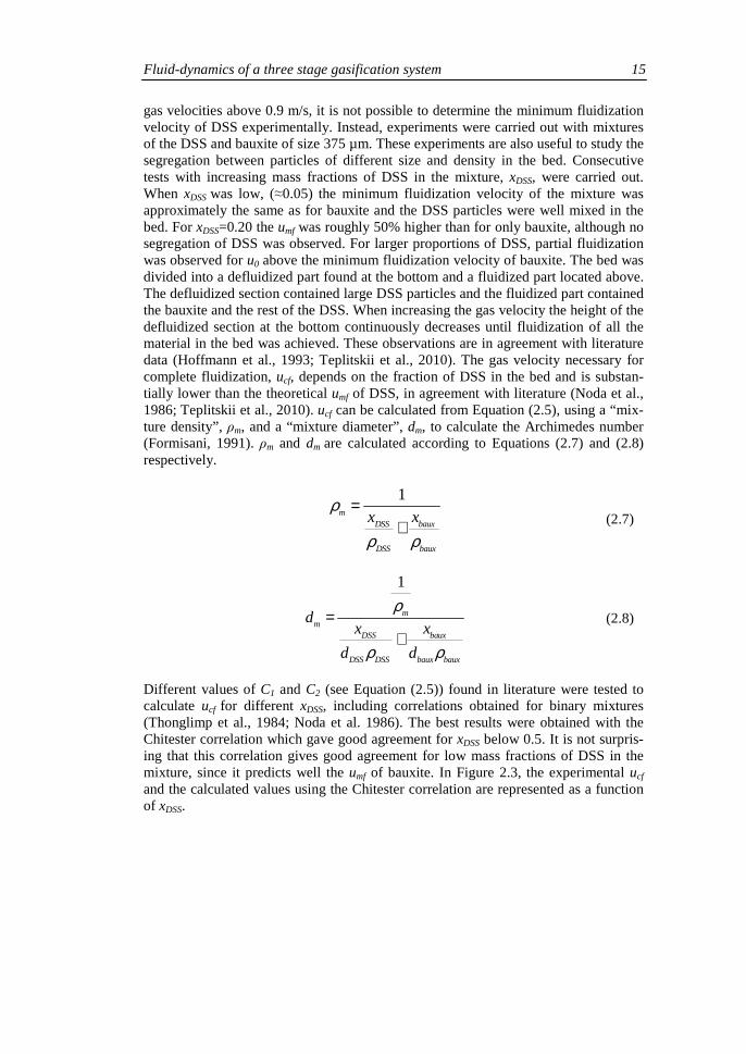
gas velocities above 0.9 m/s, it is not possible to determine the minimum fluidization velocity of DSS experimentally. Instead, experiments were carried out with mixtures of the DSS and bauxite of size 375 µm. These experiments are also useful to study the segregation between particles of different size and density in the bed. Consecutive tests with increasing mass fractions of DSS in the mixture, xDSS, were carried out. When xDSS was low, (≈0.05) the minimum fluidization velocity of the mixture was approximately the same as for bauxite and the DSS particles were well mixed in the bed. For xDSS=0.20 the umf was roughly 50% higher than for only bauxite, although no segregation of DSS was observed. For larger proportions of DSS, partial fluidization was observed for u0 above the minimum fluidization velocity of bauxite. The bed was divided into a defluidized part found at the bottom and a fluidized part located above. The defluidized section contained large DSS particles and the fluidized part contained the bauxite and the rest of the DSS. When increasing the gas velocity the height of the defluidized section at the bottom continuously decreases until fluidization of all the material in the bed was achieved. These observations are in agreement with literature data (Hoffmann et al., 1993; Teplitskii et al., 2010). The gas velocity necessary for complete fluidization, ucf, depends on the fraction of DSS in the bed and is substan-tially lower than the theoretical umf of DSS, in agreement with literature (Noda et al., 1986; Teplitskii et al., 2010). ucf can be calculated from Equation (2.5), using a “mix-ture density”, ρm, and a “mixture diameter”, dm, to calculate the Archimedes number (Formisani, 1991). ρm and dm are calculated according to Equations (2.7) and (2.8) respectively.
Different values of C1 and C2 (see Equation (2.5)) found in literature were tested to calculate ucf for different xDSS, including correlations obtained for binary mixtures (Thonglimp et al., 1984; Noda et al. 1986). The best results were obtained with the Chitester correlation which gave good agreement for xDSS below 0.5. It is not surpris-ing that this correlation gives good agreement for low mass fractions of DSS in the mixture, since it predicts well the umf of bauxite. In Figure 2.3, the experimental ucf and the calculated values using the Chitester correlation are represented as a function of xDSS.
1ρ
ρ ρ
=+
mDSS baux
DSS baux
x x
(2.7)
1
ρ
ρ ρ
=+
mm
DSS baux
DSS DSS baux baux
dx x
d d
(2.8)

16 Chapter 2
Figure 2.3: Experimental velocity of complete fluidization, ucf, as a function of the weight fraction of DSS in mixtures of DSS and bauxite (375 µm), xDSS, compared with values cal-culated from the Chitester correlation and properties of the solids mixture given by Equa-
tions (2.7) and (2.8).
2.5. Bed porosity
The porosity in a FB depends both on the properties of the particles employed and on the gas velocity. In this section bed porosities obtained experimentally for different particles and gas velocities are presented and compared to values calculated using correlations from literature.
2.5.1. Experimental procedure
The bed porosity is commonly determined from the pressure variations along the bed:
Here, the bed porosity was determined from time averaged pressures measured at different heights in the bed. Measurements were carried out both in the reactor and in the seal, both during batch and continuous experiments. Bauxite of sizes 375 µm and 650 µm and ofite of sizes 375 µm and 750 µm were employed. During the batch tests the mass of solids in the bed was constant, varying the expanded bed height as a func-tion of gas velocity. During the continuous tests the bed height was maintained con-stant through overflow, varying the mass of solids in the bed depending on the gas velocity.
0.2
0.3
0.4
0.5
0.6
0.7
0.2 0.3 0.4 0.5 0.6
u cf,
m/s
xDSS
Experimental
Calculated
( )1ρ ε= −p
dPg
dz (2.9)
Fluid-dynamics of a three stage gasification system 17
2.5.2. Results and discussion
Experimental results:
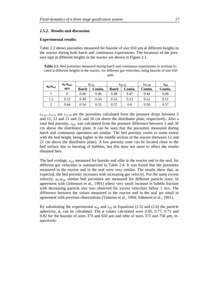
Table 2.3 shows porosities measured for bauxite of size 650 µm at different heights in the reactor during both batch and continuous experiments. The locations of the pres-sure taps at different heights in the reactor are shown in Figure 2.1.
Table 2.3. Bed porosities measured during batch and continuous experiments in sections lo-cated at different heights in the reactor, for different gas velocities, using bauxite of size 650
µm.
u0/umf u0-umf,
m/s ε3-12 ε12-21 ε21-30 εbd
Batch Contin. Batch Contin. Contin. Contin. 1 0 0.46 0.46 0.48 0.47 0.44 0.46
1.5 0.22 0.49 0.50 0.53 0.53 0.51 0.51
2 0.44 0.54 0.55 0.57 0.6 0.58 0.57
ε3-12, ε12-21 are ε21-30 are the porosities calculated from the pressure drops between 3 and 12, 12 and 21 and 21 and 30 cm above the distributor plate, respectively. Also a total bed porosity, εbd, was calculated from the pressure difference between 3 and 30 cm above the distributor plate. It can be seen that the porosities measured during batch and continuous operation are similar. The bed porosity varies to some extent with the bed height, being higher in the middle section of the reactor (between 12 and 21 cm above the distributor plate). A low porosity zone can be located close to the bed surface due to bursting of bubbles, but this does not seem to affect the results obtained here. The bed voidage, εbd, measured for bauxite and ofite in the reactor and in the seal, for different gas velocities is summarized in Table 2.4. It was found that the porosities measured in the reactor and in the seal were very similar. The results show that, as expected, the bed porosity increases with increasing gas velocity. For the same excess velocity, u0-umf, similar bed porosities are measured for different particle sizes. In agreement with (Johnsson et al., 1991) where very small increase in bubble fraction with decreasing particle size was observed for excess velocities below 1 m/s. The difference between the values measured in the reactor and in the seal are small in agreement with previous observations (Tannous et al., 1994; Johnsson et al., 1991). By substituting the experimental umf and εmf in Equations (2.3) and (2.4) the particle sphericity, ø, can be calculated. The ø values calculated were 0.85, 0.77, 0.73 and 0.82 for the bauxite of sizes 375 and 650 µm and ofite of sizes 375 and 750 µm, re-spectively.

18 Chapter 2
Table 2.4. Bed porosities measured for bauxite and ofite during batch tests carried out in the reactor and in the seal
Bauxite 375 µm
Reactor Seal u0/umf u0-umf, m/s εbd u0/umf u0-umf, m/s εbd
1.0 0 0.46 1.0 0 0.47 1.5 0.11 0.50 1.5 0.11 0.50 2.0 0.22 0.53 2.0 0.22 0.54 3.0 0.44 0.55 2.5 0.33 0.57 4.0 0.66 0.59 3.0 0.44 0.59
Bauxite 650 µm
u0/umf u0-umf, m/s εbd (reactor) εbd (seal) 1.0 0 0.47 0.47 1.5 0.22 0.51 0.53 2.0 0.44 0.56 0.56
Ofite 375 µm
u0/umf u0-umf, m/s εbd (reactor) εbd (seal) 1.0 0 0.46 0.44 2.0 0.14 0.50 0.48 3.0 0.28 0.54 0.55 4.0 0.42 0.57 0.61
Ofite 750 µm
u0/umf u0-umf, m/s εbd (reactor) εbd (seal) 1 0.0598 0.45 0.46
1.7 0.322 0.53 0.54 Theoretical calculation of the bed porosity:
It is well known that the porosity is a function of the bubble fraction in the bed, δb, and the porosity in the emulsion phase, εe, that can be assumed equal to that of mini-mum fluidization (εe=εmf):
According to the original two-phase theory of fluidization (TPT), all the gas flow in excess of the minimum fluidization velocity passes through the bed in the form of bubbles.
uv is the visible bubble flow, that can be expressed as a function of the bubble velocity, ub: uv=δb·ub, δb is the fraction of the bed volume occupied by bubbles. The two-phase
( )1ε δ ε δ= − +bd b mf b (2.10)
0= −v mfu u u (2.11)

Fluid-dynamics of a three stage gasification system 19
theory has been modified to account for gas flow through the bubbles by adding a throughflow term (Johnsson et al.,1991):
The bubble velocity, ub can be expressed as the sum of the visible bubble flow and the relative rise velocity of a single bubble in an infinite bed, ubr (Davidson et al. 1963):
Combining Equations (2.12) and (2.13) an expression for the bubble fraction can be obtained.
ubr can be calculated as a function of the bubble diameter, db, (Davidson et al. 1963):
The bubble diameter can be calculated according to Darton et al. (1977):
The throughflow can be expressed as:
Different methods for calculating χ have been proposed (Johnsson et al.,1991; Zijerveld et al., 1997). According to the TPT; χ=1. The method proposed by Johnsson et al. is given by Equations (2.18) and (2.19).
dp in Equation (2.19) is expressed in mm. Zijerveld et al. employed the following expression to calculate χ:
0δ= = − −v b b mf tfu u u u u (2.12)
0δ= + = − − +b b b br mf tf bru u u u u u u (2.13)
0
1
1δ =
+− −
bbr
mf tf
u
u u u
(2.14)
( )0.50.711=br bu gd (2.15)
( ) ( )( )0.80.4 0.5 0.2
00.54 4 −= − +b mf bdd u u h A g (2.16)
( )( )01 χ= − −tf mfu u u (2.17)
( )0.40.5
2 4χ = + bdf h A (2.18)
( )( )( ) 0.33
2 00.26 0.7exp 3.3 0.15−
= + − + −p mff d u u (2.19)
0.181.45χ −= Ar (2.20)

20 Chapter 2
Other methods for calculating the bubble fraction as a function of the bed expansion ratio, Rbd, have been proposed (Hespbasli, 1998; Babu et al., 1978).
(Hespbasli, 1998), gave the following expression, valid for Rbd>1:
and (Babu et al. 1978) proposed:
The Babu correlation was obtained using a large number of literature data obtained for coal and related materials.
Once the bubble fraction has been determined, the bed porosity can be obtained ac-cording to Equation (2.10). Table 2.5 gives the particle size and density and gas ve-locities employed to obtain the different correlations for εbd found in literature.
Table 2.5. Experimental parameters employed to obtain different correlations for εbd found in literature
Correlation dp, µm ρp, kg/m3 u0-umf, m/s Geldart Classification Johnsson 150-790 2600 0-3 B
Hepbasli 593 1233
1836 2486
0.05-0.70 B D
Babu 250-4000 50-2900 0-39·umf B and D The bed porosity has been calculated for the materials employed in this study as a function of the gas velocity using the methods presented above. Figure 2.5 shows a comparison between the experimental values measured in the reactor and the calculat-ed values for the different materials. The results in Figure 2.5 show that the correla-tions proposed by Babu et al. and Johnsson et al. gave the best agreement and can be employed to predict the bed porosity as a function of the gas velocity for bauxite and ofite. The mass of solids in the bed can be calculated as a function of the bed porosity using Equation (2.9). The TPT and the Hepbasli model overpredict the experimental values of bed porosity and the correlation employed by Zijerveld gave generally too low values.
11δ = −b
bdR (2.21)
( )0.1110.129
00.5482= −bd p mfR d u u (2.22)
( )( )0.738 1.006 0.376
0
0.126 0.937
14.311
ρ
ρ
−= +
mf p p
bd
g mf
u u dR
u (2.23)

Fluid-dynamics of a three stage gasification system 21
(a) (b)
(c) (d)
Figure 2.5: Experimental bed porosities measured in the reactor and calculated values using different models, (a): bauxite 375 µm; (b): bauxite 650 µm; (c): ofite 375 µm ; (d): ofite 750
µm.
2.6. Mixing of solids
The mixing of solids was studied by measuring the distribution of residence times of DSS particles in the seal. As explained in section 2.2, in the real system, there will be a separation wall in the reactor, like in the seal, but in the cold model there is no wall in the reactor. In order to have measurements representative of the reactor and seal in the real system, the experiments in the cold model, for characterizing the mixing of solids, were carried out in the seal.
2.6.1. Experimental procedure
The mixing of DSS particles was studied. As discussed in section 2.4.2 it was not possible to fluidize a bed containing only DSS, so mixtures of DSS and bauxite were employed. The actual proportion of inert material to be employed in the real system will be determined in a later stage during operation of the system. Therefore, at the moment, various mixtures are treated. Both the reactor and seal were filled with a
0.4
0.45
0.5
0.55
0.6
0.65
0.7
1 1.5 2 2.5 3 3.5 4
Bed
poro
sity
, εb
d
u/umf
Experimental Calculated TPTCalculated Johnsson Calculated ZijerveldCalculated Hepbasli Calculated Babu
0.4
0.45
0.5
0.55
0.6
0.65
0.7
1 1.5 2
Bed
poro
sity
, εb
d
u/umf
Experimental Calculated TPTCalculated Johnsson Calculated ZijerveldCalculated Hepbasli Calculated Babu
0.4
0.45
0.5
0.55
0.6
0.65
0.7
1 2 3 4
Bed
por
osity
, εb
d
u/umf
Experimental Calculated TPTCalculated Zijerveld Calculated HepbasliCalculated Babu Calculated Johnsson
0.4
0.45
0.5
0.55
0.6
0.65
0.7
1 1.5 2
Bed
por
osity
, εb
d
u/umf
Experimental Calculated TPTCalculated Johnsson Calculated ZijerveldCalculated Hepbasli Calculated Babu

22 Chapter 2
mixture of DSS and bauxite. Experiments were carried out during continuous opera-tion. The gas velocities in the reactor and in the seal were sufficiently high for the whole bed to be mixed without visible segregation of the DSS. A batch of 20 g of spray painted DSS was initially loaded into the upper part of the downcomer. During the experiments the solids leaving the seal were collected in the char converter and samples were taken every 30 s. The mass of bauxite and painted and non-painted DSS in each sample was determined and it was confirmed that xDSS in the bed remained practically constant during the whole test. The pressure drop in the bed was measured to check that the total mass of solids in the bed was constant during the experiment and approximately equal to 1 kg. The duration of each test was 5 min and the gas velocity employed was 0.75 m/s.
2.6.2. Results and discussion
Figure 2.6 shows the variation of the mass fraction of painted DSS particles in the bed, with the non-dimensional time, t/τ for three different mass fractions of DSS in the bed. τ is the spatial time defined as mbd/Fs, being Fs the solids flow rate and mbd the total mass of solids in the bed. mt is the mass of painted particles in the bed at time t and m0 is the initial mass of painted particles added to the bed at time 0. Figure 2.6 also shows mt/m0 calculated assuming perfect mixing (PM).
Figure 2.6: Fraction of painted DSS remaining in the bed, mt/m0 as a function of the dimensionless time, experimental values obtained for three xDSS and values calculated
assuming perfect mixing (PM).
It can be seen that the curves are approximately the same for the three mass fractions of DSS in the bed studied and equal to the curve calculated assuming PM. This means that perfect mixing of the solids in the bed can be assumed and the residence time distribution of the solids can be calculated as a function of τ using Equation (2.24):
xDSS=0.66
xDSS=0.59
xDSS=0.57
0
0.1
0.2
0.3
0.4
0.5
0.6
0.7
0.8
0.9
1
0 1 2 3 4
mt/m
0
t/τ
PM
Fluid-dynamics of a three stage gasification system 23
τ (τ=mbd/Fs) can be estimated for given operating conditions by calculating mbd using Equation (2.9) and the bed porosity using correlations from literature (Johnsson et al.,1991; Babu et al., 1978) (as discussed in section 2.5).
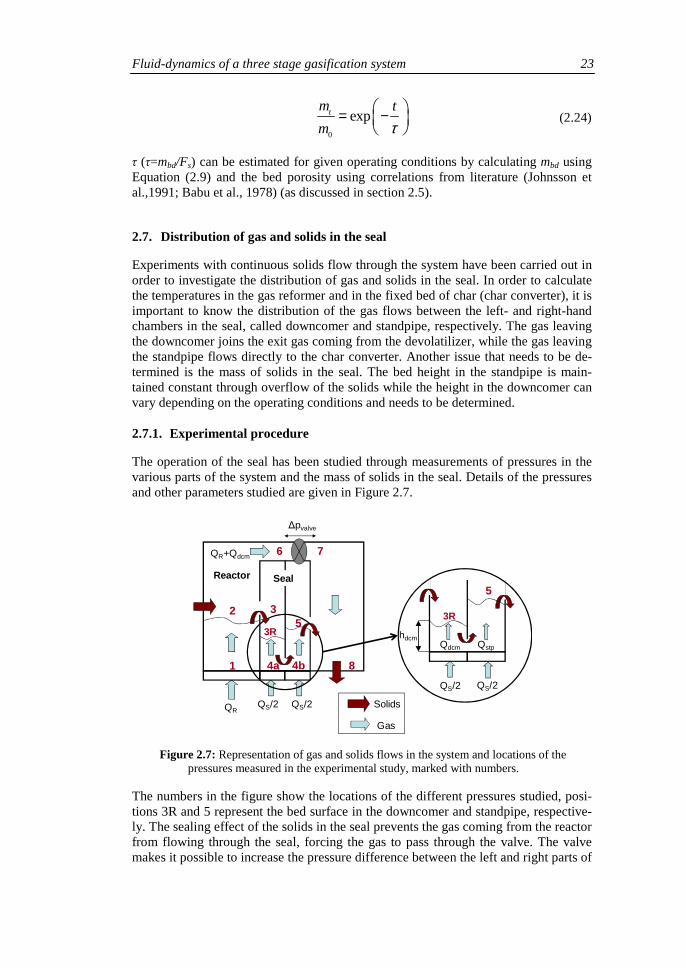
2.7. Distribution of gas and solids in the seal
Experiments with continuous solids flow through the system have been carried out in order to investigate the distribution of gas and solids in the seal. In order to calculate the temperatures in the gas reformer and in the fixed bed of char (char converter), it is important to know the distribution of the gas flows between the left- and right-hand chambers in the seal, called downcomer and standpipe, respectively. The gas leaving the downcomer joins the exit gas coming from the devolatilizer, while the gas leaving the standpipe flows directly to the char converter. Another issue that needs to be de-termined is the mass of solids in the seal. The bed height in the standpipe is main-tained constant through overflow of the solids while the height in the downcomer can vary depending on the operating conditions and needs to be determined. 2.7.1. Experimental procedure
The operation of the seal has been studied through measurements of pressures in the various parts of the system and the mass of solids in the seal. Details of the pressures and other parameters studied are given in Figure 2.7.
Figure 2.7: Representation of gas and solids flows in the system and locations of the pressures measured in the experimental study, marked with numbers.
The numbers in the figure show the locations of the different pressures studied, posi-tions 3R and 5 represent the bed surface in the downcomer and standpipe, respective-ly. The sealing effect of the solids in the seal prevents the gas coming from the reactor from flowing through the seal, forcing the gas to pass through the valve. The valve makes it possible to increase the pressure difference between the left and right parts of
∆pvalve
1
2 3
3R5
8
6 7
QS/2 QS/2QR
Qdcm Qstp
QS/2 QS/2
3R
5
hdcm
4a 4b
Solids
Gas
Reactor Seal
QR+Qdcm
0
expτ
= −
tm t
m (2.24)

24 Chapter 2
the system. The position of the valve can be varied between five positions, here called O, A, B, C and D, O meaning completely open. If the valve is partly closed a pressure difference between the two chambers in the seal, called downcomer and standpipe, is created. QR and QS are the gas flows fed to the reactor and seal, respectively. As can be seen in Figure 2.7, in all the tests, QS was divided equally, so half of the gas flow was fed to the downcomer and the rest to the standpipe. The gas flows in the left- and right-hand chambers in the seal are called Qdcm and Qstp, respectively. Correlations that give the pressure drop in the valve, ∆Pvalve, as a function of the gas flow though it for the different positions have been obtained previuously. In Figure 2.7 it can be seen that the gas flow through the valve is QR+Qdcm. When the valve is completely open, ∆Pvalve=0, and the only pressure drops in the system are caused by the solids in the reactor and in the seal, so in this case: P2=P3=P5=P6=P7=P8≈Patm. The manipulated variables in the system are the gas flows fed in the reactor, QR and in the seal, QS and the position of the valve and the objective is to determine Qdcm, Qstp and the height of the bed in the downcomer, hdcm. Qdcm and Qstp were determined using pressure meas-urements at the different locations shown in Figure 2.7 and hdcm, was is recorded visu-ally.
2.7.2. Results and discussion
Table 2.5 shows values of manipulated and measured variables, for continuous opera-tion tests carried out using bauxite of size 375 µm as bed material. The measured variables shown are the pressures at the bottom of the bed in the reactor, P1, in the downcomer, P4a, and in the standpipe, P4b, hdcm and ∆Pvalve.
Table 2.5. Continuous operation tests using bauxite of 375 µm as bed material, values of manipulated and results of measured variables.
Manipulated Measured
Number of experiment QR QS
Position of the valve
∆Pvalve P1,
mbar P4a,
mbar P4b,
mbar hdcm, m
4 50 12 0 0 44 19 19 0.15 5 75 12 0 0 39 19 19 0.15 6 50 12 A 7.2 44 19 19 0.10 7 75 12 A 13.0 39 19 19 0.07 8 50 6 0 0 44 24 24 0.15 9 75 6 0 0 39 24 24 0.15 10 60 12 A 9.6 42 19 19 0.09 11 60 18 A 10.4 42 16 16 0.07 12 60 12 B 13.1 42 19 19 0.07 13 60 18 B 14.5 42 16 16 0.05
The data in Table 2.5 indicate that for all the tests, P4a≈P4b, meaning that at the bot-tom of the seal there is no pressure drop between the two chambers. In the following, the pressure at the bottom of the seal will be referred to as P4. When the valve is com-pletely open, the pressures in the seal are not influenced by the gas flow in the reactor, only by the conditions in the seal. When the valve is partly closed, the pressures in the seal are affected by QR because an increase in QR leads to an increase in ∆Pvalve. Ac-cording to the pressure balance in the system it is possible to have different gas veloc-ities in the two chambers in the seal, because the pressure drop in the downcomer depends both on the gas velocity and on the bed height and the bed height is variable.

Fluid-dynamics of a three stage gasification system 25
Also different sizes of bubbles in the two chambers have been observed visually dur-ing operation. The relationship between the pressure drops in the valve and in the two chambers in the seal can be expressed as:
This means that if ∆Pvalve increases either ∆Pdcm should decrease or ∆Pstp should in-crease and if ∆Pvalve=0, ∆Pstp=∆Pdcm. Comparing the results from tests 4, 5, 8 and 9 it can be seen that when ∆Pvalve=0, hdcm≈hstp, and since the pressure drop is the same in the two chambers also the gas flows should be the same. So it is concluded that when the valve is completely open, hdcm≈hstp and Qdcm≈Qstp. The effect of an increase in ∆Pvalve for a given QS can be seen by studying the results of the tests 4-7. It can be seen that when ∆Pvalve increases, P4 does not change, which means that ∆Pstp is the same. This means also that the gas flows in the two chambers remain unchanged and instead the increase in ∆Pvalve is compensated by a decrease in hdcm giving a lower ∆Pdcm. From tests 10-13 it can be seen that when the valve is partly closed and QS increases, ∆Pvalve increases, which means that Qdcm increases. The results also show that P4 and hdcm decrease. The decrease in P4 means that the gas flow in the standpipe also has increased leading to lower ∆Pstp. In order to study the distribution of the gas flows between the downcomer and standpipe, the correlations that give the pressure drop in the valve as a function of the gas flow obtained previously were employed to calculate Qdcm and Qstp, for tests 10-13. The results are shown in Table 2.6.
Table 2.6. Gas flows in the downcomer and standpipe calculated as a function of ∆Pvalve
Number of experiment ∆Pvalve Qdcm, Nm3/h (calc.) Qstp, Nm3/h (calc.) 10 9.6 5.9 6.1 11 10.4 9.0 9.0 12 13.1 5.8 6.2 13 14.5 9.3 8.7
The results in Table 2.6 indicate that Qdcm≈Qstp. From the results of the continuous operation tests it can be concluded that the gas flow fed to the seal is divided equally between the two chambers so that Qdcm=Qstp. If the pressure is the same in the two columns, the bed heights are also the same. If the pressure in the left part of the sys-tem is increased leading to a pressure difference between the two chambers in the seal, this is compensated by a decrease of the bed height in the left-hand chamber, so the system evolves to a state where the pressures in the system are kept as low as possible.
Experimental pressure diagrams in the system obtained using bauxite of 650 µm as bed material are shown in Figure 2.8. Figure 2.8(a) shows pressures measured with the valve completely open (∆Pvalve=0), while Figure 2.8(b) represents pressures meas-ured for ∆Pvalve>0.
4 8− = ∆ = ∆ + ∆stp dcm valveP P P P P (2.25)
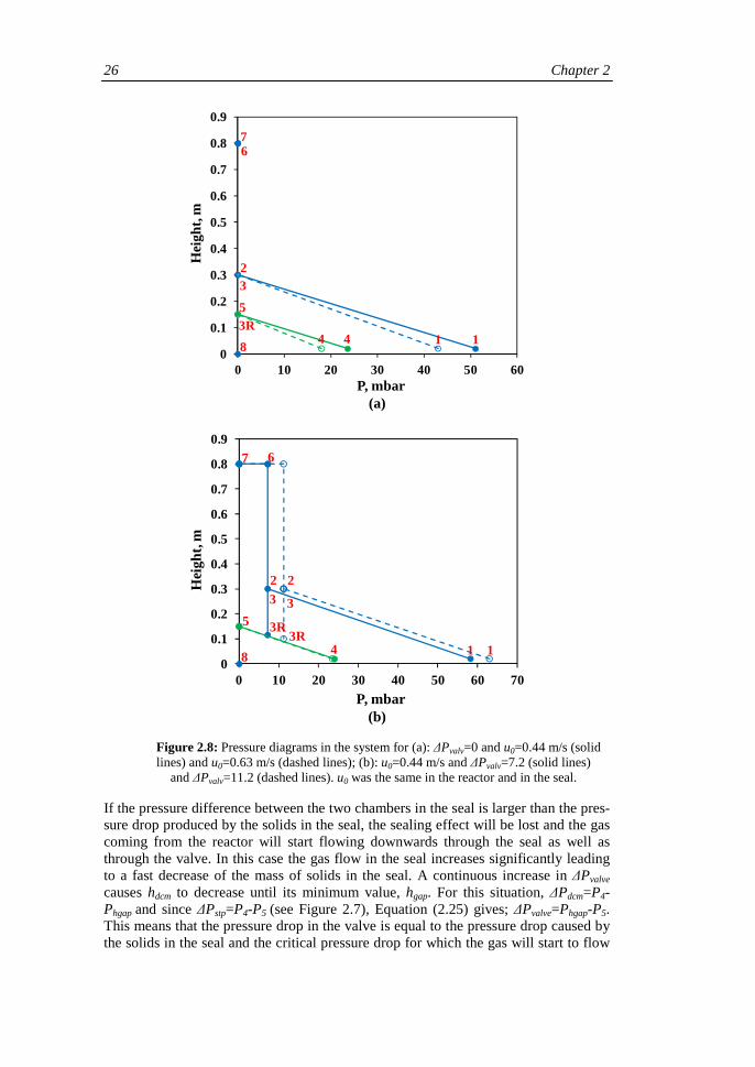
26 Chapter 2
(a)
(b)
Figure 2.8: Pressure diagrams in the system for (a): ∆Pvalv=0 and u0=0.44 m/s (solid lines) and u0=0.63 m/s (dashed lines); (b): u0=0.44 m/s and ∆Pvalv=7.2 (solid lines)
and ∆Pvalv=11.2 (dashed lines). u0 was the same in the reactor and in the seal.
If the pressure difference between the two chambers in the seal is larger than the pres-sure drop produced by the solids in the seal, the sealing effect will be lost and the gas coming from the reactor will start flowing downwards through the seal as well as through the valve. In this case the gas flow in the seal increases significantly leading to a fast decrease of the mass of solids in the seal. A continuous increase in ∆Pvalve causes hdcm to decrease until its minimum value, hgap. For this situation, ∆Pdcm=P4-Phgap and since ∆Pstp=P4-P5 (see Figure 2.7), Equation (2.25) gives; ∆Pvalve=Phgap-P5. This means that the pressure drop in the valve is equal to the pressure drop caused by the solids in the seal and the critical pressure drop for which the gas will start to flow
14 1
2
4
5
3
3R
67
80
0.1
0.2
0.3
0.4
0.5
0.6
0.7
0.8
0.9
0 10 20 30 40 50 60
Hei
ght,
m
P, mbar
3
3R1
2
1
2
4
5
3
3R
67
80
0.1
0.2
0.3
0.4
0.5
0.6
0.7
0.8
0.9
0 10 20 30 40 50 60 70
Hei
ght,
m
P, mbar

Fluid-dynamics of a three stage gasification system 27
through the seal, ∆Pcrit, has been reached. Figure 2.9 represents the pressure diagram of the system for the critical condition, hdcm=hgap.
Figure 2.9: Pressure diagram of the system when hdcm=hgap and calculation of ∆Pcrit.
From Figure 2.9 the following relations can be deduced from trigonometry:
and ∆Pcrit can be calculated from:
According to Equation (2.27), apart from the dimensions of the seal (h5 and hgap) ∆Pcrit depends on P4 which only depends on QS, not varying with QR. The critical pressure drop has been measured for two different gas flows in the seal. Table 2.7 shows a comparison between the experimental ∆Pcrit and the values calculated by using Equations (2.26) and (2.27). As can be seen in Table 2.7, there is good agree-ment between the experimental and calculated values. It is concluded that the design of the seal should be done by careful selection of the height of the standpipe and the size of the gap for the design value of QS. Equation (2.27) is helpful for the design of the system.
h5
hgapα
α
∆Pcrit
P4
4
5 5
∆=
−
crit
gap
PP
h h h (2.26)
5
4
5
−∆ =
gap
crit
h hP P
h (2.27)

28 Chapter 2
Table 2.7. Experimental and calculated ∆Pcrit values for two different gas flows in the seal.
QS P4 ∆Pcrit experimental ∆Pcrit calculated 13 24 22 22.4 19 18 16 16.8
2.8. Conclusions
The flows of solids and gas in a three stage FBG have been studied. The minimum fluidization velocities were measured for different materials and particle sizes, includ-ing mixtures of DSS and bauxite. Various correlations from literature were compared with measurements and good agreement was obtained using proper correlations. The bed porosity was measured experimentally for different materials and gas veloci-ties. It was found that the bed porosity can be assumed to be constant throughout the bed. The models proposed by Babu et al. (1978) and Johnsson et al. (1991) gave good agreement with the experimental results of the bed porosity, enabling estimation of the mass of solids in the bed. The mixing of the solids in the seal was investigated and it was concluded that perfect mixing of the solids can be assumed, so the residence time distribution of the solids can be calculated from Equation (2.24). This enables modeling of the conversion of solids in the bed, being of special importance for estimating the extent of char gasifi-cation. The distribution of the gas flow in the seal between the downcomer and standpipe was studied during continuous operation, showing that for all the operating conditions the gas was divided equally between the two chambers. If the pressure in the left part of the system is raised, this increase in pressure is compensated by a decrease in the bed height in the downcomer, so the system evolves to a state of minimum pressure. The critical pressure difference between the downcomer and the standpipe for which the seal stops working was determined experimentally and an expression for estimating the critical pressure difference was obtained, given by Equation (2.27). The theoretical methods and correlations developed and treated in this chapter allows understanding of the three stage gasification system and will be used to model the gasifier in chapter 5.

Chapter 3
Devolatilization in fluidized bed
Devolatilization is a key conversion stage during gasification and combustion of bio-mass fuels. Knowledge of yields and composition of volatiles is especially relevant for fuels with high volatiles content such as biomass and waste. When biomass is devolatilized, light gases and tars represent 70–90% of the total mass fed, whereas only 10–30% is char (Neves et al., 2011). In a FBG, the yield of char is useful to de-termine the bed size and the carbon conversion efficiency achieved in the reactor. Determination of the tar yield is essential since high tar content limits the gas applica-tion. This chapter includes an experimental study of the devolatilization in FB of different biomass and waste fuels including wood pellets, dried sewage sludge (DSS), meat and bone meal (MBM), compost from municipal solid waste (MSW) and two agricultural residues, here called agricultural residue 1 and agricultural residue 2. The distribution of products obtained during the devolatilization in N2-atmospheres and, the influence of the composition of the fluidizing gas were studied. The results obtained for DSS will be employed in chapter 5 to model the system. Before presenting the experimen-tal procedure and results, theoretical aspects of devolatilization are treated.
3.1. Theoretical aspects of devolatilization
The products of devolatilization of biomass are usually lumped into light gases which include CO, CO2, H2, CH4 and other light hydrocarbons, liquids, including tars and water and char. Char is a carbonaceous solid that remains after thermal decomposition of the fuel.
The distribution of products obtained during devolatilization is a consequence of both the primary generation due to the thermal decomposition of the fuel and secondary reactions involving the produced volatiles. Secondary reactions may occur homoge-neously or heterogeneously, both inside the fuel particle and in the reaction furnace. Devolatilization experiments are usually conducted in inert atmosphere, using N2 or He as carrier gas for the evolving volatiles. During devolatilization, the produced volatiles are transported out of the fuel particle by convective flux. This convective flux carries away the volatiles from the particle before reacting with the surrounding gas and it prevents contact between the surrounding gas and the fuel particle. Secon-dary tar reactions include thermal cracking, reforming and polymerization reactions leading to soot formation. Also water-gas shift reaction may occur. The extent of extraparticle thermal cracking of tars is influenced by both temperature and gas resi-dence time. These reactions are important at temperatures above 500-600 ºC and at

30 Chapter 3
high temperatures they may occur to a significant extent even for residence times as low as 0.1 s (Morf and Hasler, 2002). The presence of reactive gases may influence secondary reactions during devolatilization and so the yields and distribution of the species generated. In addition, the mode of devolatilization affects the structure and reactivity of the produced char. Consequently, if the gases measured should be repre-sentative of the volatiles leaving the devolatilizing particle, secondary reactions should be minimized. This is achieved by reducing the gas residence time and the concentration of volatiles in the reactor by increasing the flowrate of carrier gas and reducing the initial mass of fuel added.
Primary generation is influenced mainly by the composition of the fuel and by the heating rate applied to the particle. The temperature at which a material decomposes depends on the relative rates of devolatilization and heating. If the heating rate is low, for example in TGA, the different components in the fuel decompose within a narrow range of temperature and the typical mass-loss curve as a function of temperature is obtained. On the other hand, if the heating rate is high, for example in a FB, the tem-perature at which devolatilization takes place can be higher, affecting the distribution of products from primary pyrolisis. An increase in heating rate has shown to give lower char yields (Di Blasi, 2009).
Different laboratory devices have been used to characterize devolatilization: packed bed furnace (Di Blasi et al., 1999), thermogravimetric apparatus (TGA) (Raveendran et al., 1996; Rao and Sharma, 1998) or FB (van den Aarsen, 1985; Jand and Foscolo, 2005; Jiang and Morey, 1992) and other devices such as drop-tube reactor, heated-grid furnace, etc. Both heating rates and peak temperatures applied vary between the different devices. TGA is usually employed when devolatilization kinetics are to be obtained. In TGA, very small samples and very fine particle sizes are used and the heating rates are low (typically 5-40 ºC/min). Under these conditions, heat transport limitations are minimized, which is a necessary condition when measuring pyrolysis kinetics. Drop tube furnace has also been applied to obtain devolatilization kinetics at temperatures above 450 ºC (Kersten et el., 2005). Much kinetic data on biomass de-volatilization has been published over the years although there is great variation be-tween the data given by different authors.
Particle size influences the heating rate and thus the distribution of primary devolatili-zation products. It can also influence the product distribution through secondary in-trapartile volatiles reactions. For thermally thin particles, where no temperature gradi-ents are present, drying and devolatilization occur in sequence and homogeneously throughout the particle, while for thermally thick particles, important intraparticle temperature gradients exist and the processes of drying an devolatilization may occur at different times in different parts of the particle, and this enhances contact between evolving moisture and volatiles and, in addition, the volatiles have to pass through a hot char layer before leaving the particle. Intraparticle tar reactions have been found to reduce liquid yields (Boronson et al., 1989; Scott and Piskorz, 1984) and char has been found to enhance themal cracking of tars (Boronson et al., 1989), leading to the formation of more char. When looking at the influence of particle size, one has to keep in mind that the volatiles generation during devolatilization can produce high pressures within the particle, which can lead to fragmentation of large particles. Fine fuel particles allow determination of the intrinsic kinetics of the chemical pyrolysis, because of uniform temperature and negligible transport resistance throughout the

Devolatilization in FB 31
fuel particle. This is the so-called kinetic regime. In contrast, for large particles the devolatilization rate tends to be limited by the internal heat transfer through the parti-cle, depending mainly on the effective thermal conductivity; then the particle is not heated isothermally, and this affects the rate of devolatilization and the product distri-bution. When the external particle surface is subject to high temperature, as in an FB, external heat diffusion may also affect the rate of devolatilization. In addition, mass transfer by the release of volatiles may influence the devolatilization rate, but it usu-ally plays a secondary role.
In order to predict the behavior of FB gasifiers and combustors, pyrolysis and devola-tilization data should be obtained at high temperature and heating rate using particle sizes in the range of the industrial application (Boronson et al., 1989; Hajaligol et al., 1982; Nunn et al., 1985; Rath et., 2002). Though, many studies have been undertaken in TGA, using low or moderate heating rates, or using flash pyrolysis conditions, where the heating rates are very high, and the temperature range of interest is from 300 to 700 °C (Di Blasi, 2008; Neves et al., 2011). In addition, in both cases the fuel particle size used for the experiments is fine, typically below 200 µm. In FB gasifica-tion and combustion, mm-sized particles are used, the temperature is higher than in flash pyrolysis (750–900 °C) and the heating rate is higher than in TGA or other lab devices. Therefore, when data are taken from TGA or flash pyrolysis to represent the behavior of biomass devolatilization in FB, some correction should be applied.
Devolatilization studies on biomass and waste found in literature show that the prod-uct yields depend to a large extent on the composition of the material employed, so extrapolating devolatilization data from one fuel to another is questionable. The prod-uct distribution obtained from various types of biomass has been studied as a function of the cellulose, hemicellulose and lignin contents (Di Blasi et al., 2001; Mohan et al., 2006). Catalytic effects of different mineral compounds may also influence the prod-uct yields. Results obtained with DSS in FB (Fonts et al., 2009) showed that the CO and CO2 concentrations in the gas can differ considerably between sewage sludges with different composition. Much work has been done for wood (van den Aarsen, 1985; Jand and Foscolo, 2005; Nunn et al., 1985; Boronson et al., 1989; Rath et., 2002; Kersten et el., 2005). Comparatively less work exists on characterization of contaminated biomass, residues and wastes (McDonnell et al., 2001; Scott et al., 2007). Pyrolysis studies found in literature usually report yields of char, tar and gas as well as main gas species, although, sometimes also yields of water and different inor-ganic contaminants and composition of tar can be found.
As a result of the many factors involved, theoretical prediction of devolatilization is complex. Recent reviews include detailed discussion of the various factors affecting the devolatilization behavior of fuel particles in both lab devices (Neves et al., 2011; Di Blasi, 2008; Kersten et el., 2005; Gómez-Barea and Leckner 2010) and commer-cial fluidized beds (Gómez-Barea and Leckner 2010). A devolatilization model aims at obtaining the rates of generation of the different volatile products, as well as the yields of char, tar, light gas and water and the composition of the tar and gas fractions. Many different reaction schemes have been used to describe devolatilization. The most simple models represent pyrolysis by a single reaction or by a combination of series and parallel reactions. First order kinetics of the different reactions are com-monly used, although nth order expressions have also been employed (Grønli et al., 2002). Thermal decomposition of wood has commonly been expressed as a single

32 Chapter 3
process, including three paralell reactions for char, gas and liquid formation, the so-called “Shafizadeh” scheme (Kersten et el., 2005). The kinetic parameters are ob-tained by regression of yield versus temperature data. The calculated activation en-ergy is lower for char formation than for liquid and gas formation, predicting lower char yields for higher pyrolysis temperatures. Also distributed activation energy mod-els where the activation energy is described by a continuous distribution function have been applied to fuel devolatilization (Stengsen et al., 2001) These models can be applied to obtain yields of tar, gas and char, but they do not predict the composition of volatiles. The models have been employed together with detailed transport models (particle models) to predict devolatilization times and product yields, but it has been concluded that it is not possible to accurately predict product yields for biomass pyro-lysis from the available kinetics (Kersten et el., 2005). Other more complicated struc-tural models have been developed for prediction of yields and composition of the main products (Gómez Barea and Leckner, 2010).
Despite a considerable effort has been made to model devolatilization processes (Chan et al., 1985; Agarwal et al., 1986; Peters et al., 2003), an experimental ap-proach is mostly used when facing the prediction of reactor performance in biomass combustion and gasification (Gómez-Barea and Leckner 2010). Detailed particle models are not frequently used for fluidized bed simulations. Instead semi-empirical- or simplified particle models are used. Simplified models estimate the time of com-plete devolatilization by considering the rate-limiting phenomena. The yields of char and volatiles and the composition of volatiles are not predicted but they are estimated separately by empirical relations based on experimental data together with mass bal-ances.
Empirical data or particle models can be applied to FB models together with some limiting cases for mixing. For instance, in a bubbling FBG, when the vertical trans-portation (segregation) of fuel particles is rapid compared to devolatilization, most of the devolatilization takes place at the bed surface because it is assumed that the parti-cles keep floating once they have reached the bed surface. In such a case, the gas produced is directly influenced by the gas yields obtained by devolatilization. In the other limiting situation, when the devolatilization is rapid compared to vertical fuel mixing, most of volatiles are released in the bottom zone of the bed. In this case, the gas from devolatilization can be considered as initial gas conditions for the process all the way up the bed.
The aim of this study is to obtain devolatilization data useful for FBG modeling. The devolatilization of various biomass and waste fuels was carried out in FB using the same experimental method. This enables comparison between the different fuels. The distribution of products and conversion rate in N2 atmosphere were measured and the influence of the composition of the fluidizing gas was studied. Also secondary gas phase reactions was investigated by measuring the kinetics of the water gas shift reac-tion (WGSR). The characterization of primary and secondary tar is out of the scope of this work, but it is included in another thesis carried out in the same project.
3.2. Experimental Three main aspects were investigated, the devolatilization in N2-atmosphere, the in-fluence of the composition of the fluidizing gas and kinetics of the WGSR. The devolatilization in N2-atmosphere was studied using three different types of experi-
Devolatilization in FB 33
ments. First, experiments for measuring the yields of char and main light gas compo-nents, CO, CO2, CH4 and H2 were performed and then the water yield was measured in dedicated tests. Experiments were also carried out to characterize the shrinkage and fragmentation patterns of the fuels during devolatilization. The influence of the com-position of the fluidizing gas was investigated using CO2−N2 and H2O−N2 mixtures as fluidizing gas. The different types of experiments carried out are listed below: • Devolatilization in N2-atmosphere
• Determination of yields of char and light gas components and devolatilization times.
• Determination of yields of water • Characterization of the shrinkage and fragmentation of the particle
• Influence of the composition of the fluidizing gas • Kinetics of the WGSR 3.2.1. Material
Table 3.1 shows the chemical characterization of the six fuels used in this study. Commercial wood pellets cylindrically shaped with a mean diameter of 6 mm were used. The particle density of wood pellets was 1300 kg/m3. The MBM, compost from municipal solid waste (MSW) and agricultural residue 2 were received as powders. The agricultural residue 2 received was milled to a size <6 mm and afterwards, the fines with size <500 µm were separated. The agricultural residue 2 as received had high moisture content so it was dried in an oven at 60 ºC for 48 hours before storage. In order to enable devolatilization of MBM, compost and agricultural residues 1 and 2 in FB, avoiding entrainment of material, pellets were prepared from these materials. Pellets were prepared manually by compacting respectively: 1 g of MBM together with 0.56 g of water, 2.1 g of compost and 1 g of each agricultural residue in a cylin-drical mould with a diameter of 1 cm and applying a pressure of 50 bar. The pellets made were dried in an oven for 24 hours before being used in the experiments. Dried anaerobically digested sewage sludge (DSS) was received from an industrial drying plant processing the sludge from sewage treatment plants. Table 3.2 shows the parti-cle size distribution of the DSS as received. The particle density was 1450 kg/m3. As received DSS comprises roughly 98% (mass basis) in the size range of 2.00−4.00 mm. In this work the size range 4.00-5.00 mm (average 4.5 mm) was studied as representa-tive of behavior of the largest DSS granulates. In addition, a finer range 1.00−1.40 mm (average 1.2 mm), was studied to represent the conversion of fine granulates and to obtain kinetic parameters. Two different inert bed materials were employed in the tests, ofite, a silicate sub-volcanic rock having a density of 2600 kg/m3 and an average size of 0.5 mm and bauxite with density 3300 kg/m3 and mean particle size of 0.375 mm.

Tab
le 3
.1. P
roxi
mat
e an
d e
lem
en
tal a
nal
yses
of t
he
fuel
s st
ud
ied
.
W
ood
pelle
ts
DS
S g
ranu
late
s M
BM
A
s re
ceiv
ed
Dry
bas
is
Dry
ash
-fr
ee b
asis
A
s re
ceiv
ed
Dry
bas
is
Dry
ash
-fr
ee b
asis
A
s re
ceiv
ed
Dry
bas
is
Dry
ash
-fr
ee b
asis
LH
V (
MJ/
kg)
1
7.08
1
8.39
1
8.52
1
1.18
1
2.47
2
1.94
9
.20
13.
21
14.
16
HH
V (
MJ/
kg)
18.
42
19.
65
19.
79
12.
25
13.
41
23.
59
10.
42
14.
01
15.
02
C %
wt
- 4
9.47
4
9.80
-
30.
88
54.
32
- 3
3.78
5
6.03
H
%w
t -
5.7
9 5
.83
- 4
.36
7.6
7 -
3.7
1 6
.15
N %
wt
- 2
.03
2.0
4 -
4.7
6 8
.37
- 1
.83
3.0
4 S
%w
t -
0.0
6 0
.60
- 1
.24
2.1
8 -
0.6
8 1
.13
O %
wt
- 4
1.94
4
2.22
-
15.
61
27.
46
- 2
0.29
3
3.66
M
oist
ure
%w
t 6
.28
- -
8.6
5 -
- 2
5.62
-
- A
sh %
wt
0.6
7 0
.71
- 3
9.42
4
3.15
-
29.
54
39.
71
- V
olat
iles
%w
t 7
5.89
8
0.98
8
1.56
4
7.28
5
1.75
9
1.03
3
9.86
5
3.59
8
8.89
F
ixed
C %
wt
17.
16
18.
31
18.
44
4.6
6 5
.10
8.9
7 4
.98
6.7
0 1
1.11
C
ompo
st
Agr
icul
tura
l re
sidu
e 1
Agr
icul
tura
l res
idue
2
A
s re
ceiv
ed
Dry
bas
is
Dry
ash
-fr
ee b
asis
A
s re
ceiv
ed
Dry
bas
is
Dry
ash
-fr
ee b
asis
A
s re
ceiv
ed
Dry
bas
is
Dry
ash
-fr
ee b
asis
LH
V (
MJ/
kg)
9.2
0 1
3.21
1
4.16
1
3.91
1
5.14
1
7.42
5
.29
18.
95
22.
80
HH
V (
MJ/
kg)
10.
42
14.
01
15.
02
15.
37
16.
73
19.
26
7.2
4 2
0.01
2
4.0
8 C
%w
t -
33.
78
56.
03
- 4
2.03
4
8.39
-
48.
31
58.
13
H %
wt
- 3
.71
6.1
5 -
5.0
5 5
.82
- 4
.91
5.9
1 N
%w
t -
1.8
3 3
.04
- 0
.90
1.0
4 -
1.8
4 2
.21
S %
wt
- 0
.68
1.1
3 -
0.0
8 0
.10
- 0
.22
0.2
6 O
%w
t -
20.
29
33.
66
- 3
8.79
4
4.66
-
27.
83
33.
49
Moi
stur
e %
wt
25.
62
- -
8.1
1 -
- 6
3.85
-
- A
sh %
wt
29.
54
39.
71
- 1
1.89
1
3.14
-
6.1
1 1
6.89
-
Vol
atile
s %
wt
39.
86
53.
59
88.
89
68.
58
74.
63
85.
92
22.
06
61.
03
73.
43
Fix
ed C
%w
t 4
.98
6.7
0 1
1.11
1
1.42
1
2.23
1
4.08
7
.98
22.
08
26.
57

Devolatilization in FB 35
Table 3.2. Particle size distribution of as received DDS.
Sieve size, mm Mass fraction, % >5 0.75 4–5 0.28
2.8–4 54.86 2–2.8 39.44 1.4–2 3.70 1–1.4 0.71 0.5–1 0.21 <0.5 0.05
3.2.2. Experimental setup
Two different experimental rigs were employed in the experiments. The two experi-mental setups are operated in the same way and they have similar components, only differing in size. The two different lab-scale bubbling FB reactors employed are made of stainless steel and consist of three parts: a preheating section, a reaction part (bed), and a freeboard. The reactor is surrounded by an electrical oven and is equipped with 4 thermocouples and two controllers, allowing the control of temperature in the bot-tom bed and freeboard. The main dimensions of the two reactors are given in Table 3.3.
Table 3.3. Main dimensions of the two experimental rigs employed.
The experimental setup is represented in Figure 3.1. The system is prepared for using different gas mixtures as fluidizing gas. Steam was generated by instantaneously vaporizing a fixed flow of water. The steam generated was mixed with the other gases before entering the reactor. The gas flows were adjusted by means of mass-flow con-trollers, whereas the flow of water was adjusted by a peristaltic pump, which was calibrated before each test. The system is equipped with two ball valves that allow fuel batches to be fed from the upper part of the reactor. The fuel falls through a stain-less steel pipe to the upper part of the bed. Downstream of the reactor, the gas passes through a cyclone where any entrained material is collected and then through a line with different units for gas cleaning. The aim of the gas cleaning line is to avoid dep-osition of tar compounds within the probe and to protect the gas analyzer. The com-position of the gas was measured continuously by a Siemens analyzer using a non-dispersed infrared method for CO, CO2 and CH4 measurements and thermal conduc-tivity and paramagnetic methods for H2 and O2 measurements, respectively. The sig-nals from the analyzer are transmitted to the computerized data acquisition system, where they are monitored and registered.
Reactor 1 Reactor 2 Reactor diameter, mm 27 51
Reactor height, mm 150 200
Freeboard diameter, mm 52 81
Freeboard height, mm 200 250
Power oven, kW 4.6 10.0

36 Chapter 3
Figure 3.1: Representation of the experimental setup
3.2.3. Experimental procedure
Determination of yields of char and light gas components during devolatilization in N2-atmosphere
The procedure applied during the experiments for determining yields of light gas and char was the following:
1. The FB reactor was heated by the electrical furnace to the desired test temperature under continuous flow of pure nitrogen.
2. The flow of nitrogen was adjusted to establish the desired fluidizing velocity.
3. A batch of fuel was fed to the reactor.
4. The devolatilization process was monitored until no CO, H2, CO2 or CH4 was de-tected in the gas (3-10 minutes depending on the material being devolatilized).
5. At the end of the test, air was fed into reactor to burn the remaining char.
The gas yield (overall or accumulated) of different species was calculated as the ac-cumulated amounts of CO, CO2, CH4 and H2 detected by the analyzer during
Fuel
N2 CO2
H2O
T
P
T
P
FreeboardGas Analyzer
GasCleaning
FB
Electricaloven
MassFlow
Controllers

Devolatilization in FB 37
devolatilization. The char yield was calculated as the total amount of carbon measured as CO2 and CO during the combustion of the produced char.
Determination of water yield during devolatilization in N2-atmosphere
For determination of the amount of water formed during devoltilization, the fuel was devolatilized with N2 as fluidizing gas and the gases leaving the reactor passed through six impingers with isopropyl alcohol maintained at -20 ºC. The amount of water was then determined using Karl-Fischer titration. The batch size employed in these experiments (30 g) was higher than for the other experiments (1-3 g) to ensure that the concentration of water in the isopropyl alcohol was sufficiently high to have accurate measurements. An increase in batch size during devolatilization from 3 to 30 g could affect the results, so the total mass of fuel employed in each experiment (30 g) was divided into batches of 5 g, that were devolatilized in sequence.
Characterization of shrinkage and fragmentation patterns
For studying the shrinkage and fragmentation of the pellet, the fuel batch was devolat-ilized under N2 flow using the same procedure as for the previously described devolatilization experiments, but instead of burning the produced char, after devolatilization, the oven was switched off and the char was cooled down under a reduced N2 flow. Then the material was examined to check the size and shape of the particles.
Influence of the composition of the fluidizing gas on devolatilization
These tests were carried out in the larger experimental rig (see reactor 2 in Table 3.3) using N2−CO2 and N2−H2O mixtures as fluidizing gas. The objective is to study the influence of the composition of the fluidizing gas during devolatilization on the prod-uct distribution and conversion rate. The procedure followed during the devolatilization experiments with different fluidizing gases is described in the follow-ing. First, the reactor was heated to the desired temperature with a continuous flow of air. Once this temperature was reached, the fluidizing gas was switched to N2 to purge the oxygen. Afterwards, the composition and flow rate of the fluidizing gas were established and the batch of fuel was fed to the reactor. During these experiments both devolatilization and gasification of char take place, so the conditions of the feed gas were maintained for approximately 25 minutes, which is enough for the devolatilization to be complete and for part of the produced char to react with the steam or CO2. Afterwards, the feed gas was switched to air to burn the remaining char.
A blank test was performed to assess the effects of mixing in the gas exit line by in-jecting a certain flow of CO2 into the fluidization gas (pure N2) in a port situated in the upper part of the FB. The effect of mixing was well characterized by a first order model, with a time constant equal to 13 s. This value was used to correct the concen-trations of the light gas components measured by the gas analyzer.
Kinetics of the WGSR
The kinetics of the WGSR in the laboratory FB was measured without fuel and inert bed material in the reactor. Different gas mixtures containing N2 and two or more of the following reactive gas components: CO2, H2, CO and H2O were fed to the reactor.

38 Chapter 3
The composition of the gas at the exit of the reactor was measured continuously by the gas analyzer (as explained above) and when a constant gas composition was reached various gas samples were taken and additional measurements of the gas com-position were made using a micro-GC. First a number of blank tests were carried out by injecting a certain flow of CO2 into the fluidization gas (pure N2). The results of the tests where the CO2 was injected just below the distributor plate and at the exit of the reactor were compared and it was found that the reactor added a pure time delay, so that plug flow could be assumed in the reactor.
The stoichiometry of the WGSR is:
2 2 2+ +→←
i
d
k
kCO H O CO H (3.1)
The rates of the direct and inverse reactions have often been expressed using first order kinetics with respect to the reactive gases (Chen et al., 1987; Biba et al., 1978). The formation of CO can be expressed as:
( )2 2 2 2 2 2
= − = −CO i CO H D CO H O i CO H CO H Or k C C k C C k C C KC C (3.2)
Being K the equilibrium constant :
= D
i
kK
k (3.3)
K is calculated as a function of temperature using the following expression (Yoon et al., 1978):
39580.0265exp=
KT
(3.4)
The rate of formation of CO can be expressed as a function of the concentrations of the gas components in the feed gas and the conversion of CO2, xCO2:
( )( ) ( )( )( )2 2 2 2 2 2 2 2 2 2
1= − − − + +f f f f f f fi CO CO H CO CO CO CO CO H O CO COCOr k C x C C x K C C x C C x (3.5)
The sub index f refers to the concentration of the different gas species in the feed gas. Assuming plug flow, as discussed above, the mass balance over the reactor is ex-pressed as:
2
2
2
0
τ = ∫CO
f
x
CO
CO
CO
dxC
r (3.6)

Devolatilization in FB 39
The temperature is kept unchanged throughout the reactor, so ki is constant and substi-tuting Equation (3.5) in Equation (3.6) and after rearrangement, an expression for calculating ki is obtained:
( )( ) ( )( )2
2
2
2 2 2 2 2 2 2 2 2 20 1
τ=
− − − + +∫CO
f
f f f f f f f
i x
CO
CO
CO CO H CO CO CO CO CO H O CO CO
kdx
CC x C C x K C C x C C x
(3.7)
Equation (3.7) can be employed to calculate ki from the feed gas concentrations and the conversion of CO2 measured during the experiments and kd can then be obtained from Equation (3.3).
3.2.4. Operating conditions
Experiments were conducted varying operating parameters such as reactor tempera-ture, fluidizing velocity, particle size and the size of the fuel batch. Table 3.4 summa-rizes the fuel conversion experiments carried out, including information about the experimental rig, fuel and operating conditions employed.
Table 3.4. Experimental rig, fuel and operating conditions employed during the different
experiments.
Type of experiment Experi-
mental rig Fuel
Tempera-ture, ºC
Composition fluid-izing gas
Fluidiza-tion ve-locity, m/s
Batch size, g
Gas and char yield (devolatilization in N2)
Reactor 1
Wood pellets
750, 800, 850, 900
100 % N2 0.8 1, 2
MBM 750, 800, 850, 900
100 % N2 0.8 1
Compost 750, 800, 850, 900
100 % N2 0.8 2.1
DSS 750, 800, 850, 900
100 % N2 0.55, 0.8 2
Reactor 2
Agricultur-al residue 1
750, 825, 900
100 % N2 0.5 3
Agricultur-al residue 2
750, 825, 900
100 % N2 0.5 3
Water yield (devolatilization in N2)
Reactor 2 Agricultur-al residue 1
750, 825, 900
100 % N2 0.5 30
Influence of fluidizing gas composition
Reactor 2 Agricultur-al residue 1
750, 825, 900
55%N2+45%H2O, 60%N2+40%CO2
0.5 3
Kinetics WGSR Reactor 2 - 750, 825,
900
3-10% CO2+ 0-5% CO+4-9%
H2+0-20% H2O+N2 (the rest)
0.5 -

40 Chapter 3
3.3. Results and discussion
3.3.1. Shrinking and fragmentation behavior
Figure 3.2 shows the pictures of the various fuels prior to devolatilization and the corresponding char obtained after devolatilization.
(e)
Figure 3.2: Pictures of (a) Meat and bone meal pellet and the char generated after devolatilization. (b) Wood pellets and the corresponding char obtained after devolatilization
at various temperatures. (c) Compost pellets and char obtained after devolatilization. (d) DSS granulates (as received), char after devolatilization and ash after complete combustion.
(e) pellets of a agricultural residue 1 and the char generated after devolatilization.
For DSS, the ash obtained after complete combustion is also shown. The figure pro-vides a qualitative judgment of the fragmentation behavior during devolatilization of the fuels tested. MBM pellets (Figure 3.2(a)) showed severe fragmentation. The orig-inal shape and volume of the pellet were reduced during devolatilization and a recog-
(b)(a)
(d)
(c)

Devolatilization in FB 41
nizable skeleton was no longer observed at the end of the process, in agreement with previous work (McDonnell et al., 2001). Wood pellets (Figure 3.2(b)) and compost pellets (Figure 3.2(c)) were subjected to significant shrinking during devolatilization while fragmentation was not observed. The original shape of DSS granulates re-mained after both devolatilization and combustion (Figure 3.2(d)) though some shrinkage occurred during the process, in agreement with previous findings (Scott et al., 2007). The pellets of a agricultural residue 1 broke into a limited number of pieces and some shrinkage was also observed (Figure 3.2(e)).
3.3.2. Devolatilization in N2-atmosphere
Figure 3.3 show the yields of char, gas and condensate referred to the carbon, hydro-gen and oxygen contained in the dry and ash free fuel, obtained during the devolatilization of wood, MBM, DSS as received and compost in reactor 1.
(a) (b)
(c)
Figure 3.3: Yields of char (a) condensate (b) and gas (c) obtained during the devolatilization of wood (◊), MBM (□), DSS (○) and compost (+).
Wood
MBM
DSS Compost
0
10
20
30
40
50
750 800 850 900Temperature, ºC
Con
dens
ate
yiel
d, w
t %
Wood
MBM
DSS
Compost
8
10
12
14
16
18
20
22
750 800 850 900Temperature, ºC
Cha
r yi
eld,
wt %
Wood
MBM DSS
Compost
40
50
60
70
80
90
750 800 850 900Temperature, ºC
Gas
yie
ld, w
t %

42 Chapter 3
The char yield was obtained from the CO and CO2 measured during the combustion of char, the gas yield includes the CO, CO2, CH4 and H2 measured during devolatilization and the condensate yield was calculated by difference and includes tar, water and light hydrocarbons (other than methane). Figure 3.4 show the yields of char, gas and condensate obtained during the devolatilization of agricultural residue 2 in reactor 2.
Figure 3.4: Light gas, condensate and char yields, referred to the carbon, hydrogen and oxygen contained in the dry and ash free fuel obtained during devolatilization of agricul-
tural residue 2, note that the light gas yield is shown on the right-side vertical axis. The water yield was only measured for the devolatilization of agricultural residue 1. For this fuel, the products were divided into gas, char, water and tar. The tar yield was calculated by difference and includes tar and light hydrocarbons (other than methane). Figure 3.5 show the yields of char, gas, water and tar, referred to the carbon, hydro-gen and oxygen contained in the dry and ash free fuel, obtained during the devolatilization of agricultural residue 1 in reactor 2. The repeatability was reasonably good for all fuels with the exception of compost. The lower repeatability observed for compost was attributed to the heterogeneity of the material. As expected (Jand and Foscolo 2005; Hajaligol et al., 1982; Nunn et al., 1985; Fagbemi et al., 2001) the gas yield increases with temperature, whereas the condensate and char yield decrease for all fuels. Though, the char yields varied less with temperature than the condensate and gas yields, being practically constant for some of the fuels. For wood, the decrease of the condensate yield with temperature was less pronounced than for the other materials, consistent with previous work (Di Blasi et al., 1999), arguing that the tar from wood is less reactive than tar from various agricultural residues. Somewhat similar conclusions were made in (Rath et al., 2002), observing that some tars from the pyrolysis of wood were practically unaltered even under very high temperature and residence time. For all the materials studied, the char yields obtained were close to the fixed carbon content (daf basis) given by the proxi-mate analysis (see Table 3.1). The char yield is expected to be closely related to the
30
35
40
45
50
55
60
65
10
15
20
25
30
35
40
750 825 900
Ga
s yi
eld,
% w
eig
ht
Co
nden
sate
and
cha
r yie
lds,
% w
eigh
t
Temperature, ºC
CharCondensateGas

Devolatilization in FB 43
biomass composition, especially to the lignin content (Di Blasi et al., 1999; Antal et al., 2000) though, the presence of different inorganic species and physical properties, such as particle density and thermal conductivity, may also affect the product yields (Di Blasi, 1997). The highest char yield was obtained for agricultural residue 2, which is consistent, since this fuel is expected to have high lignin content. It has been point-ed out that high ash content in DSS and the presence of metals could favor gas for-mation at expenses of char formation (Fonts et al., 2009) However this is not obvious from our observations.
Figure 3.5: Light gas, water, tar and char yields obtained during devolatilization of ag-ricultural residue 1, note that the light gas yield is shown on the right-side vertical axis.
The volume fractions of the main species in the gas (CO, CO2, CH4 and H2) measured for wood, MBM, DSS and compost at the temperatures studied are represented in Figure 3.6 and figure 3.7 shows the gas composition measured during the devolatilization of the two agricultural residues employed. For all the fuels, CO is the main light gas component and the variations in gas compo-sition with temperature are generally small. Wood gave higher CO concentration in the gas than the other materials. These observations are in agreement with those given in (Di Blasi et al., 1999), where higher CO yields and were measured for wood, com-pared to various agricultural residues. Correlation of yields as a function of temperature To provide with a simple way to numerically compute the char, water, tar and gas yields, as well as the individual yields of CO, CO2, CH4 and H2 measured in this work, the product yields and gas composition were fitted to a quadratic function of tempera-ture (T in °C):
40
45
50
55
60
65
10
12
14
16
18
20
22
24
750 825 900
Gas
yie
ld, %
wei
ght
Cha
r, w
ater
and
tar y
ield
s, %
wei
ght
Temperature, ºC
Char Tar Water Gas

44 Chapter 3
0 1 2
2
= + +
i
ref ref
T Ty a a a
T T (3.8)
being yi the light gas, tar, water, condensate or char yield (in % weight), referred to the C, H and O in the daf fuel, or the CO, CO2, CH4 or H2 concentration in the light gas (volume %) and Tref=500 ºC. Equation (3.8) is useful for gasification modeling. The values of parameters a0, a1 and a2 are shown in Table 3.5.
(a) (b)
(c) (d)
Figure 3.6: Experimental composition of the main components in the gas (volume frac-tion): CO (a), CO2 (b), CH4 (c) and H2 (d), during the devolatilization of wood (◊), MBM
(□), DSS (○) and compost (+).
Wood
MBM
DSS
Compost
35
40
45
50
55
60
750 800 850 900Temperature, ºC
CO
vol
%
Wood
MBM
DSS
Compost
20
25
30
35
40
750 800 850 900Temperature, ºC
CO
2 vo
l %
Wood
MBM
DSS
Compost
4
6
8
10
12
14
16
18
750 800 850 900Temperature, ºC
H2
vol %
Wood
MBM
DSS
Compost
8
10
12
14
16
18
20
750 800 850 900Temperature, ºC
CH
4 vo
l %

Devolatilization in FB 45
(a) (b)
Figure 3.7: Composition, in volume %, of the light gas produced during devolatilization of agricultural residue 1 (a) and agricultural residue 2 (b), note that the CO concentration is
read on the right side vertical axis.
Time of devolatilization The conversion time t90 obtained for the different materials was calculated as the time needed for 90% of the total amount of gases to evolve. t90 for different materials measured in reactor 1 is shown in Figure 3.8.
Figure 3.8: Times for 90% conversion, t90, for wood (◊), MBM (□), DSS as received (○) and compost (+).
CO2
CH4
H2
CO
30
35
40
45
50
14
16
18
20
22
24
26
28
750 825 900
CO
, %
vo
lum
e
CO
2, C
H4a
nd
H2, %
volu
me
Temperature, ºC
CO2
CH4
H2
CO
47
49
51
53
55
10
12
14
16
18
20
22
750 825 900
CO
, % v
olum
e
CO
2, C
H4
y H
2,
% v
olu
me
Temperature, ºC
Wood
MBM 2
DSS
40
50
60
70
80
90
750 800 850 900Temperature, ºC
t 90,
s
Wood
MBM 2DSS
Compost
40
90
140
190
240
290
750 800 850 900Temperature, ºC
t 90,
s

T
able
3.5
. Val
ues
of t
he
fittin
g pa
ram
eter
s,
a 0, a
1 an
d a2,
in E
quat
ion
(3
.8)
calc
ula
ted
for
the
pro
du
ct y
iel
ds
and
ligh
t ga
s co
mp
o-
sitio
n ob
tain
ed d
urin
g d
evo
latil
izat
ion
of t
he
fuel
s st
ud
ied.
*
Tar
yie
ld fo
r ag
ricu
ltura
l res
idue
1
C
har
yiel
d, w
t%
Con
dens
ate
yiel
d*, w
t%
Gas
yie
ld, w
t%
Wat
er y
ield
, wt%
a 0
a 1
a 2
a 0
a 1
a 2
a 0
a 1
a 2
Woo
d
-15
.03
50
.58
-18
.09
-196
.07
30
0.86
-1
03.3
4 3
11.
10
-351
.45
12
1.43
MB
M
- 3
0,26
6
0,9
2 -2
1,4
2 7
5,8
9 2
0,0
0 -3
4,4
6 5
4,3
8 -
80,
92 5
5,8
7
DS
S
16
7.23
-1
72.3
9 4
7.4
7 -7
05.6
3 9
81.
52
-326
.63
75
7.85
-9
59.7
4 3
26.
52
Com
post
2
6.3
5 -2
1.7
6 7
.94
-32
.71
15
7.47
-7
2.0
6 1
06.
36
-135
.71
6
4.1
2
Agr
icul
tura
l Res
idue
2
28
.79
0
0
59
7.34
-6
21.4
3 1
64.
18
-224
.16
25
4.95
-5
3.6
0
Agr
icul
tura
l Res
idue
1
23
.624
1
.80
-4.4
0 -1
57.7
1 2
41.
18
-81
.21
24
4.34
-2
87.1
0
10
3.20
-1
0.2
5 4
4.1
1 -1
7.5
9
C
O v
olum
e %
C
O2
volu
me
%
CH
4 vo
lum
e %
H
2 vo
lum
e %
a 0
a 1
a 2
a 0
a 0
a 0
a 0
a 1
a 2
a 0
a 1
a 2
Woo
d 2
40.
53
-225
.12
67
.50
23
4.97
2
34.
97
23
4.97
-1
68.6
4
21
4.47
-6
2.5
1 2
34.
97
-257
.01
72
.50
MB
M
22
7,59
-
249
,96
82
,04
-160
.70
-160
.70
-160
.70
38
.73
-22
.51
4.5
3 -1
60.7
0 2
20.
28
-68
.53
DS
S
-119
.25
19
3.38
-5
8.3
0 -2
81.6
2 -2
81.6
2 -2
81.6
2 -6
0.1
3 1
00.
77
-32
.60 -2
81.6
2 3
55.
75
-107
.31
Com
post
2
26.
21
-230
.24
73
.19
-197
.17
-197
.17
-197
.17
18
.37
-5.1
2 0
.00
-197
.17 2
57.
93
-80
.30
Agr
icul
tura
l Res
idue
2
65
.41
-11
.60
-0.9
1 1
96.
29
-208
.82
6
0.5
3 3
5.9
6 7
6.4
9 -2
6.3
9 -1
25.7
4 1
43.
94
-33
.22
Agr
icul
tura
l Res
idue
1
24
0.30
-2
22.1
6 6
4.5
61
33
.76
-8.0
8 -1
.01
-156
.92 2
10.
26
-63
.40
-17
.14
19
.98
-0.1
6

Devolatilization in FB 47
As expected, the conversion times decreased with increasing temperature. Compost gave significantly longer conversion times than the other biomasses, especially at lower temperatures, while wood presented the lowest values. In Figure 3.8(b) the compost has been removed allowing clearer observations of the t90 for wood, MBM and DSS. The influence of the moisture content on the devolatilization times is ex-pected to be small since the moisture content of wood and DSS is low and MBM and compost were dried before the tests. Influence of the particle size In Figure 3.9 the time to reach 60% conversion, t60, is represented as a function of temperature for the three particle sizes of DSS studied (as received, 1.2 mm and 4.5 mm). The choice of t60 instead of t90 to compare the effect of size was made because the determination of the time to reach higher conversion than 80% led to high scatter-ing of data (in fact this occurred also in previous work (Scott et al., 2007)). As can be seen in Figure 3.9, t60 increases with increasing particle size. It is concluded that the effect of particle size is more significant than the temperature.
Figure 3.9: Time for 60% conversion, t60, for DSS as a function of temperature; DSS as received (◊), 1.2 mm particles (□) and 4.5 mm particles (∆).
Figure 3.10 shows the char (Figure 3.10(a)) and gas (Figure 3.10(b)) yields obtained for two particle sizes of DSS, 1.2 mm and 4.5 mm. The larger particles gave some-what higher char yields and slightly lower gas yields, in agreement with previous works (Jand and Foscolo, 2005; Rapagnà and Latif, 1997). The effect of particle size on the gas composition, however, was found very small.
For the wood pellets, the diameter was kept constant (6 mm), but the length of the pellet was varied. Several tests were carried out varying the pellet length maintaining the batch size and no significant effects were found either on product yields or on conversion times.
0
5
10
15
20
25
30
35
750 800 850 900Temperature, ºC
t 60,
s

48 Chapter 3
(a) (b)
Figure 3.10: Effect of particle size and temperature on the yields of char (a) and gas (b) for DSS.
3.3.3 Influence of the composition of the fluidizing gas
In order to study the influence of the composition of the fluidizing gas, devolatilization experiments were carried out using mixtures of 45% volume of steam in N2 and 40% volume of CO2 in N2 as fluidizing gas, and agricultural residue 1 as fuel. During these experiments, both devolatilization and gasification of the produced char with steam or CO2 occur. To study the influence of the fluidizing gas on devolatilization it is therefore important to be able to separate these two processes. To visualize the different stages of fuel conversion, sample mass loss curves were calcu-lated for the tests using different fluidizing gases. Figure 3.11 shows the sample mass loss curves obtained with the three different fluidizing gas compositions at 825 ºC. Figure 3.11 represents m(t)/m0 as a function of time, being m0 the initial mass of C, H and O in the dry and ash free sample and m(t)=m0-mv(t), where mv(t) is the total mass of light gases evolved from the particle up to time t. These mass loss curves do not take into account the mass loss due to tar and water formation during devolatilization, but they are useful for visualizing the results.
Figure 3.11 shows that the mass loss curves obtained with N2-steam mixture and N2-CO2 mixture have two distinct sections with different rates of mass loss, so overlap-ping in time between devolatilization and gasification of char is limited. This result is not unexpected since the flow of volatiles out of the particle during devolatilization, prevents the fluidizing gas to penetrate into it. It can also be seen that for the first stage, when devolatilization takes place, the mass loss curves are similar for the dif-ferent fluidizing gas compositions, so the composition of the fluidizing gas does not influence the devolatilization rate. Similar results were obtained at the other tempera-tures studied (750 ºC and 900 ºC).
1.2 mm
4.5 mm
8
10
12
14
16
18
20
750 800 850 900Temperature, ºC
Cha
r yi
eld,
wt % 1.2 mm 4.5 mm
40
50
60
70
80
90
750 800 850 900Temperature, ºC
Gas
yie
ld,
wt %
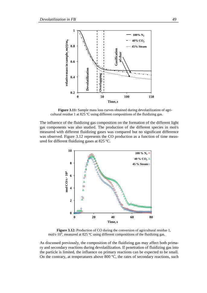
Devolatilization in FB 49
Figure 3.11: Sample mass loss curves obtained during devolatilization of agri-cultural residue 1 at 825 ºC using different compositions of the fluidizing gas.
The influence of the fluidizing gas composition on the formation of the different light gas components was also studied. The production of the different species in mol/s measured with different fluidizing gases was compared but no significant difference was observed. Figure 3.12 represents the CO production as a function of time meas-ured for different fluidizing gases at 825 ºC.
Figure 3.12: Production of CO during the conversion of agricultural residue 1, mol/s·104, measured at 825 ºC using different compositions of the fluidizing gas.
As discussed previously, the composition of the fluidizing gas may affect both prima-ry and secondary reactions during devolatilization. If penetration of fluidizing gas into the particle is limited, the influence on primary reactions can be expected to be small. On the contrary, at temperatures above 800 ºC, the rates of secondary reactions, such
0.2
0.4
0.6
0.8
1
0 50 100 150
rela
tive
ma
ss in
sa
mpl
e, m
(t)/
m 0
Time, s
Series2
Series4
Series1
Dev
ola
tiliz
atio
n
Ove
rlapp
ing
Ga
sific
atio
no
f cha
r
100% N2
40% CO2
45% Steam
100 % N2
40 % CO2
45 % Steam
0
2
4
6
8
10
0 20 40 60 80
mo
l CO
/s ·
104
Time, s

50 Chapter 3
as the WGSR can be high. If these reactions were important, the production of the different gas species should be affected by the composition of the fluidizing gas em-ployed. No such effect was observed here. One surprising results is that the produc-tion of CO is not affect by the addition of 45 % steam in the fluidizing gas. Using WGSR kinetics from literature often used for gasification modeling (Biba et al., 1978) it is predicted almost complete conversion of the CO produced during devolatilization before it leaves the reactor.
3.3.4 Kinetics of the WGSR
The kinetics of the WGSR was determined using the method to obtain the kinetic constant of the inverse WGSR, ki, presented in section 3.2.3, given by Equation (3.7). The kinetic constant of the direct reaction, kd can then be calculated from Equations (3.3) and (3.4). The Arrhenius plot of the ki values obtained experimentally is repre-sented in Figure 3.13. Also the kinetics given by Biba et al. is shown for comparison.
Figure 3.13: Arrhenius plot for the ki values measured at different temperatures and for the kinetics given by Biba et al.
The kinetic parameters obtained from the Arrhehius plot of the experimental ki values are: k0=141.3 m3/(mol s) and Ea=54.2 kJ/mol. The average ki values measured at each temperature are compared to the values calcu-lated from (Biba et al., 1978) in Table 3.6. Also the reaction rate, rCO, measured for a gas containing 10% CO2 and 9% H2 on a volume basis, the rest being N2, was com-pared to the rate calculated using the kinetics form Biba et al. (3.1) (3.2) (3.3) (3.4) (3.5) (3.6) (3.7) (3.8)
Biba et al.
This work
-1.6
-1.4
-1.2
-1
-0.8
-0.6
-0.4
-0.2
0
8.5 9 9.5 10
Ln(k
i)
1/T ·104

Devolatilization in FB 51
Table 3.6. Values of the inverse reaction constant ki, masured in this work and calculated from the kinetics given by (Biba et al., 1978).
Temperature, ºC ki, m3/(mol s)
experimental ki, m
3/(mol s) Biba et al.
rCO, mol/(m3 s) experimental
rCO, mol/(m3 s) Biba et al.
750 0.241 0.498 0.309 0.637
825 0.373 0.718 0.414 0.918
900 0.545 0.988 0.530 1.264
The reaction rates measured here are lower than the rates obtained from the kinetics given by Biba et. al. but they are of the same order of magnitude. The rates measured here are significantly higher than the rates measured without the presence of catalyst and in a reactor made of quartz (Bustamante et al., 2004), indicating that the reactor walls can act as catalyst for the reaction, in agreement with (Chen et al., 1987). In a FBG the rate of the WGSR may be higher than the rates measured here, because dif-ferent solids such as bed material and ash can have catalytic activity for the WGSR (Chen et al., 1987) and therefore using the kinetics given by Biba et al. for modeling of a FB gasifier seems reasonable. More measurements should be conducted to com-pare different materials for realistic simulation of FBG. 3.4 Theoretical analysis of the devolatilization of wood and DSS
A simple model has been developed to study the mode of conversion of a single fuel particle during devolatilization of DSS and wood in an FB. The model has been de-veloped in order to assess the influence of internal and external mass transfer and chemical kinetics on the rate of devolatilization of different fuels and particle sizes. The model does not predict the distribution of products. 3.4.1 Model development
The devolatilization of a particle is thermally driven. The evolution of the field of temperature within the particle is described by the partial differential equation of transient heat conduction with heat sources. Here, it is considered that the heat of pyrolysis is small (Scott et al., 2007; Pyle and Zaror, 1984) and that the fuel moisture does not affect the particle heat up due to the low moisture content of the fuels ana-lyzed (see Table 3.1). In this way the temperature distribution during heating up of a particle can be approximately calculated without considering the thermal effects of pyrolysis and drying. The fuel properties and the particle size were assumed to remain constant during devolatilization and equal to those of the virgin biomass (Leckner et al., 1999). This hypothesis was taken following the observation of previous work (Leckner et al., 1999) and from the results shown in Figure 3.2. Despite the variation of properties during conversion may be significant, simultaneous effects caused by variations in specific heat capacity and density during devolatilization are assumed to compensate each other for the calculations concerned in this work. An additional assumption made is that the heat flux due to the convective mass flux associated with the volatiles released is neglected (Leckner et al., 1999). Most of the assumptions made in this work have been proven to be sufficient for first estimates (Jand and Foscolo, 2005; Pyle and Zaror, 1984; Gómez-Barea and Leckner, 2010; Dupont et al., 2007). After these simplifications the temperature field at different times is obtained by solving:

52 Chapter 3
2
2ρ λ∂ ∂ ∂
= +∂ ∂ ∂
p eff
T T b Tc
t r r r (3.9)
0
∂=
∂T
r at r=0 (3.10)
( )λ
∂= −
∂eff bd
Th T T
r at r=R (3.11)
0=T T at t=0 (3.12)
where T0, Tbd are, respectively, the initial (ambient, 20 °C) and the bed temperature. b is a geometric factor, being equal to 1 for an infinite cylinder (for the simulation of wood pellets) and 2 for a sphere (for the simulation of DSS granulates). The solution of Equations (3.9)-(3.12) can be expressed in the form:
( )0
( , )( )
−Θ = =
−bd
dev
bd
T T r tT f Bi,Fo
T T (3.13)
Fo is the Fourier number defined as Fo= λeff t/(ρcpR2) and Bi is the Biot modulus for
heat transfer, defined as Bi=hR/λeff. R is the radius in spherical and cylindrical parti-cles whereas it is half of the thickness in a flat particle. Once the temperature is known, the local conversion Xdev defined as Xdev=(ρ0–ρ)/(ρ0–ρ∞), is calculated assum-ing a first order global reaction to describe the loss of mass by pyrolysis:
1 1
(1 ) ( )
ρρ ρ∞
∂ ∂= = −
− ∂ − ∂dev
dev
dev
Xk
X t t (3.14)
where kdev is a kinetic constant following the Arrhenius form:
exp= −
dev
dev dev
g
aEk A
R T (3.15)
The degree of pyrolysis conversion xdev is calculated by integrating the local conver-sion, Xdev throughout the particle:
1
0
1( ) ( , )=
+
+∫ devb
Rb
dev
bt r t
Rx r X dr (3.16)

Devolatilization in FB 53
To obtain the temperature fields within the particle and xdev at different times and the evolution of xdev with time during conversion, the model represented by Equations (3.9)-(3.16) was integrated numerically.
The effective gas-particle heat transfer coefficient, h, is calculated by considering only convection (Dupont et al., 2007) using two different correlations: the Ranz and Marshall equation (Ranz and Marshall, 1952) given in Equation (3.17) as well as a specific correlation derived for fuel conversion in FB (Equations (3.18) and (3.19)) (Leckner, 2006; Palchonok, 1998) were used. Equation (3.18) is valid for large parti-cles being converted in a FB of fine inert material, so it is applicable for wood pellets and for 4.5 mm DSS granulates. For 1.2 mm DSS granulates, Equation (3.19) devel-oped for particles of similar size to that of the inert bed particles in an FB, is applica-ble.
1/3 1/22 0.6= +p pNu Pr Re (3.17)
0.19 0.5 0.330.85 0.006= +i i iNu Ar Ar Pr (3.18)
0.39 0.336 0.117= +p iNu Ar Pr (3.19)
There are significant differences between the h obtained from Equations (3.17)-(3.19). Equation (3.17) is an expression developed for single-phase flow and the values given by this expression are expected to be lower than the actual h in FB, where heat trans-fer is enhanced by the circulation of inert particles. Equations (3.18) and (3.19), on the contrary, give maximum Nu values at optimum fluidization velocity. The actual h values for the experiments in the present work is expected to be intermediate between the values given by Equation (3.17) and Equations (3.18) and (3.19) because in a small lab FB with the fuel fed at the top, it is most likely that the fuel particles stay most of the time at the bed surface during devolatilization (Leckner et al., 1999; Gómez-Barea and Leckner, 2010). Also, the heat transfer coefficient may be different in small scale fluidized beds compared to larger scales due to differences in gas flow patterns, which affects the movement of solids.
The properties for wood pellets were obtained from (Leckner et al., 1999), where commercial wood pellets with similar size were converted in an FB. The properties of DSS were estimated assuming the thermal diffusivity of DSS to be intermediate be-tween those of wood and silica (Scott et al., 2007).
Various kinetic data of kdev for wood and DSS pyrolysis are shown in Table 3.7. Olive residue is also included as representative of other biofuel materials. As seen, there is a great variation even for wood. This is explained by the way to obtain the kinetics by different researchers and also because the representation of pyrolysis by a first-order global expression is a rough approximation. As a result the choice between one ex-pression and another is difficult. This is discussed below for the specific fuels simu-lated.

54 Chapter 3
A scaling analysis to preliminary assess the limiting mode of conversion and a simpli-fied model to estimate the conversion time during FB devolatilization of wood pellets and DSS is shown in the Appendix.
Table 3.7. First-order kinetics models of pyrolysis given in literature for various fuels
Source Fuel Eadev (J/kmol)
Adev (1/s) kdev (1/s) 500 ºC 800 ºC
Davidsson et al., 2001
Wood 1.78·108 1.90·1012 1.8·100 4.2·103
Brink and Massoudi, 1978
White fir 1.05·108 2.64·105 2.1·10-2 2·100
Jand and Foscolo, 2005
Beech wood 2.05·107 1.5 6.2·10-2 1.5·10-1
Kosstrin, 1980 Sawdust 1.83·108 1.00·1013 4.3·100 1.2·104
Biagini et al., 2002 Olive residue 1.14·108 3.27·106 6.6·10-2 9.3·100
Scott et al., 2006 DSS 2.84·108 1.86·1019 1.2·100 2.8·105
3.4.2 Wood pellet simulation
Wood pellet was assumed to be an infinite cylinder, in order to apply the model de-veloped. This assumption has been shown to yield good results under FB combustion conditions as long as the length to diameter ratio is larger than 3 (Sreekanth et al., 2008). The validity of this simplification was verified since no difference was ob-served in the conversion times measured using 1 pellet of 25 mm and two pellets of 12.5 mm length.
The experimental xdev was defined as:
,
( )
∞
= voldev
vol
V tx
V (3.20)
Vvol(t) and Vvol,∞ being respectively, the accumulated mass of volatiles measured up to a time t and that after complete devolatilization.
Figure 3.14 shows the temperatures at the surface and centre of a wood pellet, calcu-lated using the model and the conversion determined experimentally from Equation (3.20) for a bed temperature of 800 ºC. The large differences between the two temper-ature curves indicate that intraparticle temperature gradients are important during devolatilization of wood pellets. In addition, it is observed that conversion is almost complete (>95%) when the particle centre is still below the bed temperature (<750ºC). This indicates that heating up of the particle greatly influences the devolatilization process.
For simulating the evolution of conversion during the devolatilization of wood pellets the apparent kinetics determined by (Jand and Foscolo, 2005) (see Table 3.7) was used because it was obtained in very similar setup and operating conditions. A com-parison between the results of the simulation and the conversion versus time curves obtained experimentally is shown Figure 3.15.

Devolatilization in FB 55
Figure 3.14: Temperatures at the surface and centre of wood pellets calculated with the model (h=160 W/(m2 K)) and experimental conversion. (Tbd=800 ºC).
Figure 3.15: Comparison between simulated (solid lines) and experimental (dashed lines) conversion curves for devolatilization of wood pellets at four bed temperatures.
The model reproduces the conversion of wood pellets fairly well during the whole range of conversion for all temperatures.
A sensitivity study was carried out varying the values of the parameters that were assumed to have the most important effect on the conversion times and whose deter-mination can be assumed to be less certain: h, λeff, Eadev, and Adev. The uncertainty related to the estimation of the cp and ρ values is assumed to be less important, be-cause their values in literature vary less than those of other parameters. For the sensi-
Tsurface
→
← ←Tcentre
0
100
200
300
400
500
600
700
800
0 20 40 60 80 100Time, s
Tem
pera
ture
, ºC
0
10
20
30
40
50
60
70
80
90
100
Con
vers
ion,
%
800ºC
750ºC
↑
850ºC↓
900ºC
↓
↑
0
10
20
30
40
50
60
70
80
90
100
10 20 30 40 50 60Time, s
Con
vers
ion,
%

56 Chapter 3
tivity study the values of the parameters were varied within a range of values found in literature. The effect of the kinetic parameters was studied by varying ±50% the Eadev and Adev values from (Jand and Foscolo 2005). The high and low h values are the values calculated from Equations (3.17) and (3.18), respectively. The effect of apply-ing other kinetics was also studied: parameters given by Brink et al., Davidsson et al.
and Kosstrin (see Table 3.6) instead of those given by (Jand and Foscolo, 2005) were used. The results of the sensitivity analysis are shown in Figure 3.16.
The results in Figure 3.16 show that both internal and external heat transfer are im-portant, which is consistent with Figure 3.14. Figures 3.16(a) and 3.16(b) also indicate that the choice of kinetic parameters is important. The fact that Edev is the most im-portant parameter in Figure 3.16(a) does not imply that the process is controlled by devolatilization kinetics. The choice of kinetic parameters will determine the tempera-ture above which the devolatilization can be considered to be fast, so even if the pro-cess is controlled by particle heat up, the kinetic parameters will have a great influ-ence on the devolatilization time, as discussed in the section 3.4.2.
Figure 3.16: Percentage variation of t90 calculated from the model (a) when varying the parameters given at the bottom of the chart, between extreme values found in literature and (b) when employing kinetic parameters given by different authors shown in Table
3.7, (□) % variation with the low parameter value, (■) % variation with the high param-eter value.
3.4.3 DSS simulation
To elucidate the way of conversion of DSS granulates the model was applied to simu-late the temperature profiles of DSS granulates with the largest and finest sizes of the DSS received (1.2 and 4.5 mm). Each graph of Figure 3.17 includes the evolution with time of the experimental conversion as well as the simulated temperature at both, particle surface and center. Figure 3.17(a) corresponds to DSS particles of 1.2 mm, whereas Figure 3.17(b) stands for DSS particles of 4.5 mm. Figure 3.17(a) shows that 1.2 mm DSS granulates are heated up so quickly that the temperature at the centre of
h λeff Edev Adev-80
-60
-40
-20
0
20
40
60
80
100
120
Parameter
% v
aria
tion
of t
90
Kosstrin (57)
Davidsson et al. (56)
Brink (55)-80
-60
-40
-20
0
20
40
60
80
100
Reference
% v
aria
tion
of t
90
Eadev

Devolatilization in FB 57
the particle is already at 790 °C when the conversion is only 10%. Moreover, the temperatures at the particle centre and at the particle surface are very similar during the whole conversion process, so that intraparticle temperature gradients are small. Figure 3.17(b) shows that for 4.5 mm DSS particles, intraparticle temperature gradi-ents are more significant than for 1.2 mm particles, but still small, so the particle heat up is mainly influenced by external heat transfer. By comparing the two graphs of Figure 3.17 it is seen that the conversion of 4.5 mm particles proceeds slower than that of 1.2 mm particles, indicating that the devolatilization rate is significantly af-fected by the particle heat up for coarse particles.
In Figure 3.17(a), it is observed that from around xdev=0.15, the pyrolysis kinetics can be considered to control the overall conversion. This is explained by the following observations: (a) the temperature gradients inside the particle are small, so Xdev can be considered to be the same throughout the particle volume and equal to xdev; (b) since the evolution of the process is still limited when the particle has approximately reached the bed temperature, Tbd, most of the volatiles can be considered to be re-leased at Tbd throughout the particle. Then the pyrolysis kinetic coefficient kdev at the bed temperature can be approximately obtained by integrating the expression in Equa-tion (3.21):
1 1( ) ln
1=
−
dev
dev b
x dev
k Tt x
(3.21)
(a) (b)
Figure 3.17: Simulated temperatures at the surface and the centre of the DSS particles (solid lines) and experimental conversion (dashed lines) at Tbd=800 °C and u=0.8 m/s. (a) 1.2 mm DSS particles, (b) 4.5 mm DSS particles (h=250 W/(m2 K) for 1.2 mm particles
and h=185 W/(m2 K) for 4.5 mm particles). For bed temperatures lower than 800 ºC (Figure 3.17(a) corresponds to devolatilization at 800 ºC) the kinetic regime will be reached at even lower conver-sions. Figure 3.18 shows txdev versus ln(1/(1-xdev)) for experiments carried out with 1.2 mm DSS particles at 750 ºC and 800 ºC. The points in Figure 3.18 are apparently
←←
→
0
100
200
300
400
500
600
700
800
0 10 20 30 40 50Time, s
Tem
pera
ture
, ºC
0
10
20
30
40
50
60
70
80
90
100
Con
vers
ion,
%
Tsurface
←Tcentre←→
0
100
200
300
400
500
600
700
800
0 20 40 60 80 100Time, s
Tem
pera
ture
, ºC
0
10
20
30
40
50
60
70
80
90
100
Con
vers
ion,
%

58 Chapter 3
arranged into two lines, suggesting that kdev for conversions below and above 0.70 are different. This means that there are two different dominating processes during DSS thermal conversion. DSS may contain a number of different material fractions with different devolatilization kinetics. As a consequence, the composition of the uncon-verted material could change during conversion, leading to a modification of the global devolatilization kinetics. Another possible explanation for the change in kinetic behavior at high conversions is the partial sintering of some material, obstructing the flow of volatiles outwards. The observed fact that the conversion rate is not affected by the bed temperature for conversions above 70−80% for 4.5 mm particles, supports this thesis. The Adev and Edev for xdev<0.7 and xdev≥0.7 obtained from Figure 3.18 are shown in Table 3.8. These values vary largely compared to those from (Scott et al., 2006), concluding that the devolatilization kinetics of the DSS tested in this work is much slower than the DSS tested by Scott et al.
Figure 3.18: Time of devolatilization to reach conversion xdev, txdev as a function of ln(1/(1-xdev)) for tests conducted with 1.2 mm DSS particles and bed temperatures be-
tween 750 ºC and 800 ºC.
Table 3.8. Values for the pre-exponential factor (Adev) and activation energy (Eadev) obtained by applying Equation (3.21) to experimental results obtained at 750 °C and 800 °C using 1.2
mm DSS particles.
Conversion range Eadev (J/kmol) Adev (1/s) 0.15≤xdev<0.7 3.63·107 4.95 0.7≤xdev≤0.9 5.35·107 16.15
The kinetic parameters in Table 3.8 were given as input to the model presented above to calculate the conversion as a function of time for as received DSS and 4.5 mm DSS particles. The results are displayed in Figure 3.19 where the simulated conversion-vs-time curves are shown for various bed temperatures. As seen the curves calculated with the model compare well with the experimental ones, indicating that the model
0
10
20
30
40
50
60
70
0.0 0.4 0.8 1.2 1.6 2.0 2.4ln(1/(1-x dev))
t xde
v, s
800 ºC, x<0.70
750 ºC, x<0.70
750 ºC, x≥0.70
800 ºC, x≥0.70

Devolatilization in FB 59
developed can be used to simulate the devolatilization process of DSS in an FB pro-vided the kinetics given in Table 3.8 is used.
(a) (b)
Figure 3.19: Conversion of DSS particles calculated from the model (solid lines) and conver-sions obtained experimentally (dashed lines). (a) as received particles (3.3 mm mean size), (b)
4.5 mm particles.
3.5 Conclusions
In this chapter, literature on devolatilization of biomass and wastes has been reviewed. It was found that the distribution of products and the conversion rate depend to a large extent on the composition of the fuel and on the operating conditions employed, mainly heating rate, temperature and particle size. Since the modeling of devolatilization and prediction of product yields in a FBG is a complex task, pseudo-empirical approach has been applied. The devolatilization of various biofuels in N2-atmosphere (wood, meat and bone meal, compost, dried sewage sludge (DSS) and two agricultural residues was studied in a lab-scale fluidized bed (FB) between 750 and 900 °C. The yields of char, condensate and light gas, as well as the gas composi-tion and the time of conversion during devolatilization were determined for the differ-ent fuels. The yields and gas composition were correlated with bed temperature for all fuels (Table 3.5). These correlations, together with the devolatilization rate are useful for modeling FBG.
A simple model was developed to understand the mode of conversion of DSS and wood pellets. The heat up of DSS particles was found to be mainly influenced by external heat transfer, while for wood pellets both internal and external heat transfer were important. The devolatilization of fine DSS particles was found to be controlled by pyrolysis kinetics during most of the conversion period, so the Arrhenius parame-ters for first-order devolatilization kinetics were determined within the lower tempera-ture range (Table 3.8). These kinetic parameters were successfully applied to simulate the conversion of larger DSS particles at different temperatures.
Experiments were carried out using N2-H2O and N2-CO2 mixtures to study the influ-ence on the results of the fluidizing gas composition during devolatilization. No sig-nificant influence was found and the overlapping in time between devolatilization and gasification of char was small. These results indicate that the product distribution
750 ºC
800 ºC←850 ºC
0
10
20
30
40
50
60
70
80
90
0 10 20 30 40Time, s
Con
vers
ion,
%
800 ºC 750 ºC
0
10
20
30
40
50
60
70
80
90
100
0 10 20 30 40 50 60Time, s
Con
vers
ion,
%

60 Chapter 3
measured in N2-atmosphere can be employed for FBG modeling and that the devolatilization and gasification of the produced char can be assumed to occur in series. These simplifications are applied in the model of the three stage gasification system in chapter 5.
Kinetics of the water gas shift reaction (WGSR) in the lab FB was investigated and the results obtained were in the same order of magnitude as kinetics found in litera-ture frequently applied to gasification modeling. The catalytic effects on the WGSR of different materials present in an FBG should be further investigated.

Devolatilization in FB 61
Appendix: Scaling analysis and estimation of the devolatilization time
A scaling estimation through dimensionless numbers is made to preliminary assess if limiting mode of conversion during FB devolatilization of wood pellets and DSS granulates can be identified using data from literature. This is done by computation of the Biot modulus for heat transfer, Bi, and Damköhler number for devolatilization, Dadev (Pyle and Zaror, 1984). Bi, defined as Bi=hR/λeff, quantifies the thermal behav-ior of the fuel particles by comparing the rates of external and internal heat transport, respectively h/(ρcpR) and λeff/(ρcpR
2). If Bi>>1, the particle heating is limited by intapartle heat transfer and if Bi<<1, the external heat transfer is rate limiting. For comparing the particle heat up and the devolatilization kinetics, when Bi>1, the Damköhler number of pyrolysis, defined as Dadev=kdevρcpR
2/λeff, that compares the rates of pyrolysis kinetics, kdev, and internal heat transfer is caulated and when Bi<1, Dadev/Bi, which compares the rates of pyrolysis kinetics and external heat transfer is used. The Dadev value depends on the temperature at which kdev is calculated. Since the temperature at which devolatilization occurs is not known a priori, Dadev is usually evaluated at the bed temperature.
The Nusselt number, Nu, obtained from Equations (3.17)-(3.19) and the correspond-ing h and Bi values calculated for wood pellets and DSS with 0.8 m/s gas velocity, at 800 ºC, are shown in Table 3.9. Since the wood pellets are cylindrically shaped, the particle diameter was replaced with ødeq in Equation (3.17), being deq the equivalent diameter, deq = (6Vp/π)
1/3 and ø the particle sphericity, ø=πdeq
2/Sp.
None of the two limiting situations given by Bi (Bi>>1 or Bi<<1) can be clearly estab-lished for the fuels and operating conditions tested in the present work. Rough guides can, however, be established: given the relatively low Bi number for DSS, the exter-nal heat transfer should have a significant influence on the particle heat up. Similar results were obtained in (Scott et al., 2007) by conducting tests with DSS particles with sizes in the range of 0.65–8 mm. In contrast, given the relatively larger Bi ob-tained for wood pellets, the internal heat transfer will greatly influence the particle heat-up and large temperature gradients will be present during the devolatilization of wood pellets. This agrees with the results obtained by (Thunman et al., 2001).
To compare the rate of heat transfer with devolatilization kinetics, the Dadev calculat-ed using the kinetics from Table 3.7 is presented in Table 3.9. The ratio Dadev/Bi for DSS particles was also calculated for the cases where Bi<1. For Dadev and Dadev/Bi, instead of a single value, a range of values is presented in Table 3.9, resulting from the various kinetics (four for wood and one for DSS) (see Table 3.7) and the two values of h. As seen Dadev is high for all cases, no matter what kinetics or correlation of h is used. The lower bound for wood Dadev (12.21) is obtained using the kinetics given by (Jand and Foscolo 2005), which yields the lowest kdev at high temperatures (see Table 3.7). Note that Dadev is computed at bed temperature so a temperature, Tdev, between T0 and Tb where Dadev becomes high is likely to exist, in other words, there is a Tdev (Tdev<Tb) above which devolatilization is very fast compared to the heat up of the particle.

Tab
le 3
.9. E
stim
ates
fo
r th
e sc
alin
g an
alys
is:
Nu
, h
, B
i, D
a dev a
nd T
dev c
alcu
late
d fo
r w
oo
d p
elle
ts a
nd D
SS
usi
ng
Eq
ua-
tion
s (
3.1
7)-
(3.1
9)
and
a g
as v
eloc
ity o
f 0.8
m/s
an
d 8
00
ºC.
Nu
(eq
11)
(eq
12)
(eq
13)
h, W
/(m
2 K)
(eq
11)
(
eq 1
2)
(eq
13)
Bi
(eq
11)
(e
q 12
)
(eq
13)
Da d
ev
Da d
ev/B
i
Woo
d pe
llets
5
.89
3.0
8
46
.67
35
6.46
0.5
4 4
.11
1
2.2
1 –
1.0
·106
D
SS
, 1.2
mm
3
.18
7
.33
18
8.19
47
1.38
0
.19
0.
47
8
.22
·10
5 – 2.
03
·106
DS
S, 4
.5 m
m
4.7
6 3
.41
7
5.0
6 3
56.
46
0
.28
1.3
7
3
.97
·10
6_ 1
.94
·107

Devolatilization in FB 63
Pyrolysis can be considered complete when the particle centre has reached Tdev (Pyle and Zaror, 1984; Leckner et al., 1999; Scott et al., 2007).
In this scenario, the devolatilization can be assumed to be completed once the particle (the center in case of thermally thick particles) has heated up to Tdev and the time of conversion can then be estimated by the time for heating a particle up to Tdev (Gómez-Barea and Leckner, 2010). This simplification can be especially useful for engineer-ing applications, for which it is often enough to predict the time of complete devolatilization. The time needed for particle heat up can be calculated by making asymptotic approximation of the two coefficients appearing in the first term of the Fourier series of the exact solution in Equation (3.13) (Ostrogorsky, 2009) to give:
2
2
1
1ln
( )
µτµ
=Θ
dev ih
dev
tT
(3.22)
Θ(Tdev) being the dimensionless temperature defined as:
0
( )−
Θ =−
bd devdev
bd
T TT
T T (3.23)
Expressions for calculating µ1 and µ2, (the two coefficients of the first term of the solution expressed in Fourier series) are shown in Table 3.10.
Table 3.10. Values of parameters µ1 and µ2 in Equation (3.22).
0 <Bi<2 2<Bi<∞
µ1 0
11+ /
a Bi
Bi a
3
4+
a Bi
Bi a
µ2
2
1+Bi
a 5
6+
a Bi
Bi a
a0 a1 a2 a3 a4 a5 a6 Plate 1 3 7 π/2 0.95 1.273 0.15
Cylinder 2 4 4 2.4048 1 1.602 0.35 Sphere 3 5 3.5 π 1.1 2 0.65
Equation (3.22) can be used for both fine and large particles. For thermally fine parti-cles, however, intraparticle temperature gradients are negligible, and a simpler ex-pression can be used to estimate tdev:

64 Chapter 3
1ln
( )τ=
Θ
dev eh
dev
tT
(3.24)
To estimate Tdev the condition Dadev=1 or Dadev/Bi=1 is used:
( )ln τ= deva
dev
g dev
ET
R A (3.25)
τ being the characteristic time for heat up, estimated by Equations (3.26) and (3.27):
2ρτ = p
eh
c R
h for Bi<1 (3.26)
( )22ρ
τλ
= p
ih
eff
c R for Bi>1 (3.27)
Figure 3.20 compares tdev/τih calculated by the approximate and numerical solutions for various values of Bi and two Θdev, showing that the approximation given in Equa-tion (3.22) is excellent for Θdev typical of FB fuel conversion at high temperature (combustion and gasification).
Figure 3.20: Comparison between tdev calculated by the approximate (lines in the figure) and numerical solution (points in the figure) for various values of Bi and two Θdev, typical of FBG.
Figure 3.21 shows a comparison between the experimental t90 and devolatilization times calculated using the approximate model described above and various pyrolysis kinetics for wood given in Table 3.7. As seen, Equation (3.22) gives a good prediction of t90 using the kinetics of Brink et al., whereas the agreement is poor when using the
0,0
0,1
0,2
0,3
0,4
0,5
0,6
0,7
0,8
0,9
1,0
0,0 1,0 2,0 3,0 4,0 5,0 6,0 7,0 8,0
t dev
/τih
Bi
dev 0,70Θ =dev 0,57Θ =
dev 0,45Θ =

Devolatilization in FB 65
kinetics of (Jand and Foscolo, 2005). The use of Kosstrin’s and Davidsson’s kinetics yields intermediate results.
Figure 3.21: Comparison between t90 obtained experimentally (●) and tdev calculated from Equation (3.22) and employing devolatilization kinetics from literature: (◊)
Davidsson et al., (∆) Kosstrin, (□) Brink, (×) Jand and Foscolo.
As explained, tdev calculated from Equation (3.24) is expected to be a good approxi-mation for the devolatilization time as long as Dadev changes rapidly with temperature once Tdev has been reached, i.e. d(Dadev)/dT>>1 for T≥Tdev. This is true as long as the activation energy of the pyrolysis reaction is greater than for heating. Since the latter is a physical process, with lower activation energy than a chemical process, the as-sumption is, in principle, reasonable. However, when pyrolysis is assumed to be de-scribed by a single first order reaction, the kinetic coefficient does not only account for a single chemical reaction, but it lumps a number of physical and chemical pro-cesses. In Figure 3.22 Dadev is represented as a function of temperature for the devolatilization kinetics given for wood in Table 3.7.
The value of Tdev is determined by the intersection of the Dadev–T curve with Dadev=1. The kinetics given by Davidsson et al. and Kosstrin give Tdev between 350 and 400 ºC, while the kinetics proposed by Brink et al., give a Tdev close to 500 ºC. As can be seen the increase of Dadev with T near Tdev is small for the kinetics proposed by Jand and Foscolo. The reason is that Jand and Foscolo’s kinetics has low activation energy (see Table 3.6), because the authors included the effect of particle size into the kinetic equation. The Kosstrin’s and Davidsson’s kinetics makes Dadev to be more sensitive to T than Brink’s kinetics (higher slopes above Tdev in Figure 3.22), but the use of Brink’s kinetics yields to better estimation of t90.
0
10
20
30
40
50
60
70
750 800 850 900Temperature, ºC
t dev
, s

66 Chapter 3
Figure 3.22: Dadev as a function of temperature for different devolatilization kinetics from literature: (◊) Davidsson et al., (∆) Kosstrin, (□) Brink, (×) Jand and Foscolo.
Dadev = 10
10
20
30
40
50
100 200 300 400 500 600 700 800Temperature, ºC
Da d
ev

Chapter 4
Conversion of char in fluidized bed gasi-fication
4.1. Introduction
The kinetics of char gasification is a key aspect when designing a fluidized bed gasifier (FBG) because the reactions of char with CO2 and H2O are slow compared to devolatilization and gas phase reactions. In most cases, conversion of char is not completed in FBG, thus reducing the process efficiency. The combustion of char often plays a minor role in directly heated gasifiers because only a fraction of the stoihiometric oxygen is fed and the char has to compete with the volatiles for the oxygen. For indirectly heated FBG, on the other hand, the knowledge of the rate of char combustion is important because the energy necessary for the devolatilization, gasification and reforming reactions is obtained from the combustion of char in a separate reactor.
In this chapter the conversion of char from dried sewage sludge (DSS) in fluidized bed (FB) was studied. This fuel was selected because it will be used as reference fuel for the development of the three-stage gasification system and the results obtained in this chapter will be implemented in the model presented in chapter 5. The main focus was made on the gasification of char with CO2 and H2O, but also the combustion of char was briefly studied. The rates of char gasification were studied by first obtaining kinetic expressions for the reactions with CO2 and H2O, separately. Then the gasifica-tion of char in gas mixtures containing both reactive gases was investigated in dedi-cated experiments, with the objective to obtain a method for modeling the conversion of char in an air-blown FBG.
4.1.1. Gasification of char in FBG
The rate of char conversion is influenced by variables, such as temperature, partial pressure of the gasifying reactants and the products, particle size, porosity, and miner-al content of the char, some of which vary with time due to chemical conversion and attrition. The rate of char gasification is expressed as:
0
1= − =C c
C
dm dxr
m dt dt (4.1)

68 Chapter 4
mC0 and mC being the mass of carbon in the char at initial time and at conversion xc, respectively. The reactivity of char is defined as the conversion rate referred to the mass of carbon in the sample at time t:
Char reactivity depends on the parent fuel and on the form of preparation, especially the heating rate and peak temperature. The reactivity of coal chars varies widely de-pending on the rank of the parent coal. Variation between chars derived from different types of biomass is even more significant, due to the differences in the nature of the biomass fuels. Biomass chars vary greatly in porosity, directionality, and catalytic activity. Therefore, caution should be exerted in applying expressions from one char to another (Buekens et al., 1985). The influence of the form of char generation on the char reactivity has been studied (Lou et al., 2001; Fushimi et al., 2003). FB or other equipment, having conditions that are as similar as possible to FB, such as laminar flow (drop tube) or entrained flow reactors, should be used to generate the char, and preferably, also to measure the char–gas reactivity without intermediate cooling. The most important parameters affecting the properties of the char generated after devolatilization are the temperature and particle heating rate (Gómez-Barea and Leckner, 2009b). The composition of the fluidizing gas used during devolatilization is assumed to only slightly affect the char generated because the high flow of volatiles released from the solid particle makes penetration of the fluidizing gas difficult (Gómez-Barea and Leckner, 2010). The char preparation method can affect both the composition and properties of the char. Pore distribution and internal surface area have a great influence on the char reactivity. For fuels with high volatile content, such as biomass and wastes, the structure of the generated char is strongly affected by devolatilization conditions. Also, deactivation of chars exposed to high temperatures has been observed (Senneca et al., 1997). In commercial FBG units, mm-sized particles are used, the temperature is in the range of 750-900 ºC and the heating rate at which the fuel is devolatilized is in the order of 100-1000 ºC/s. Then, to obtain reactivity useful for application in FBG units, the char should be generated at a high temperature and heating rate. However, physical inter-action like mass transport can lead to misinterpretations of the intrinsic kinetics (Gómez-Barea et al., 2007). This is the reason why most experimental data with O2, CO2 and H2O have been measured using TGA, fixed bed or similar devices, where it is easier than in an FB to ensure that the experiments are really carried out in the kinetic regime. In these devices, small particle size and low heating rate are often employed. Moreover, there are other processes that make it difficult to prepare the char in the laboratory to be useful for FBG. A significant reduction in char reactivity after cooling the char has also been reported (Miura et al., 1989; Liu et al., 2003). However, in most kinetics studies the char generated in the laboratory is cooled down to room temperature before conducting the char gasification tests (Matsouka et al., 2009; Chitsora et al., 1987; Sears et al., 1980; Scott et al., 2005; Nowicki et al., 2010). A great deal of research exists detailing measurements of the char gasification reactiv-ity of a variety of fuels, including coal (Miura et al., 1989; Linares-Solano et al., 1979; Liu et al., 2003; Matsouka et al., 2009) and biomass (Kojima et al., 1993; DeGroot
1
1=
−c
c
dxR
x dt (4.2)

Conversion of char in FBG 69
and Richards, 1988; Moilanen and Mühlen, 1996). Comparatively less work exists on the gasification of char from contaminated biomass, residues and wastes (Scott et al., 2005; Nowicki et al., 2010; Marquez-Montesinos et al., 2002; Gea et al., 2005). Little research has dealt with the gasification of char from dried sewage sludge (DSS) (Scott et al., 2005; Nowicki et al., 2010). It was found that char from DSS had higher reac-tivity with CO2 than chars from coal and car tires (Scott et al., 2005). The reason may be the effect of catalytic compounds (Miura et al., 1989; DeGroot and Richards, 1988; Schumacher et al., 1986), which are found in large proportions in DSS char. However, it is difficult to conclude general trends based on existing char gasification or combus-tion tests from DSS found in the literature because the chemical and physical charac-teristics of DSS may vary significantly depending on its origin. Most char gasification studies have treated the gasification with CO2 and H2O sepa-rately and less work exists regarding the gasification of char in mixtures containing both CO2 and H2O. Simultaneous gasification with CO2 and H2O has been studied for coal char (Roberts and Harris, 2007; Umemoto et al., 2011; Koba et al., 1980; Huang et al., 2010). Most of these studies performed measurements in TGA (Roberts and Harris, 2007; Umemoto et al., 2011; Everson et al., 2006; Huang et al., 2010) and only some studies have assessed how the reactivity varies with char conversion (Umemoto et al., 2011; Mühlen et al., 1985). Different kinetics models have been employed to describe the simultaneous gasification with CO2 and H2O (Roberts and Harris, 2007; Everson et al., 2006; Koba et al., 1980). Based on the higher diffusivity of H2O compared to CO2 and that catalytic compounds can affect the two reactions differently, it has been argued that different active sites can have more affinity for one of the two reactants and some kinetic models assume that CO2 and H2O react at dif-ferent active sites. The reaction rate in a mixture of CO2 and H2O can then be calcu-lated as the sum of the individual reaction rates measured in the presence of only one of the reactive gases. Other models assume that the reactants have to compete for the same active sites. For most chars, the gasification with H2O is much faster than the reaction with CO2 (Roberts and Harris, 2007; Koba et al., 1980) and at high pressure an inhibition effect of CO2 has been observed leading to a decrease in reaction rate when adding CO2 to a H2O−N2 mixture (Roberts and Harris, 2007). In some studies carried out at atmospheric pressure the assumption that the two reactions occur at different active sites has given good agreement with experimental results (Everson et al., 2006; Huang et al., 2010), while in another study, the assumption that some of the active sites are shared gave good results (Umemoto et al., 2011). Very little infor-mation is available regarding the simultaneous gasification with CO2 and H2O of chars from biomass and wastes. Here, the gasification of char in mixtures containing both CO2 and H2O has been studied in order to obtain an expression that enables cal-culation of the char conversion in an FBG. To obtain the conversion rate of a char prepared from a given fuel in a mixture of CO2 and N2 (reaction with CO2) or in a mixture of H2O and N2 (reaction with H2O), at temperature T, the following expression can be used to fit the measurements (Gómez-Barea and Leckner, 2010):
2 2/( , ) ( )=cx CO H O cr r T p F x (4.3)

70 Chapter 4
where rxc is the conversion rate at reference state of conversion. rxc accounts for the dependence of reactivity on temperature and partial pressure of gas reactant (pCO2 or pH2O), whereas F(xc) is a function taking into account the variation of the gasification rate with conversion. pCO2 stands for the partial pressure of CO2 in the CO2−N2 mix-tures used during CO2 reactivity tests and pH2O is the partial pressure of H2O in the H2O−N2 mixtures used during H2O reactivity tests. The approximation assumed in Equation (4.3) by which the conversion rate can be written as the product of two func-tions rxc (T, pCO2/H2O) and F(xc) has been shown to be valid within a specific range of operating conditions (especially within a specific temperature interval) (Ollero et al., 2002; Gómez-Barea and Leckner, 2010).
If the reactivity, R, is constant with xc the reaction is first order with respect to the mass of carbon and F(xc)=(1-xc). The variation of the char reactivity with conversion has been correlated with the inner surface area, but also other properties can affect the char reactivity. Both structural and empirical models of F(xc) have been employed in literature. A review of different models can be found in (Gómez-Barea and Leckner 2010).
The gasification reactions are governed by surface processes. For the char gasification reactions to take place, the reactive gas (CO2 or H2O) first has to be adsorbed at an active site on the surface of the char structure. The presence of CO and H2 can affect the rate of char gasification, since these compounds can adsorb on the char surface, blocking the active sites. Langmuir-Hinshelwood kinetics (Scott et al., 2005; Jüntgen, 1981) has shown to represent the char reactivity, which accounts for the observed inhibitory effects of CO and H2 (Di Blasi, 2009; Ollero et al., 2002). However, at moderate pressure and when the partial pressure of CO and H2 are not very high, the reactivity at a given conversion, can be simplified by nth order kinetics. The validity of this simplification can be verified experimentally by confirming that the order of reaction neither varies with temperature nor with degree of conversion. Assuming this simplification, rxc can be represented using the following expression:
Equations (4.3) and (4.4) allow for a simplified and practical expression to fit the measurements. However, the validity of the assumptions made to derive Equations (4.3) and (4.4) should be verified experimentally. Moreover, the reactivity (kinetic parameters and structural profile) should be obtained without diffusion effects, i.e. intrinsic reactivity. In this way, the reactivity could be used as part of a char particle model to predict the conversion in practical equipment (with a variety of char sizes and operating conditions). In this work, an expression for the intrinsic reactivity of char from DSS for both gasi-fication with CO2 and H2O (in mixtures where only a single reactant, CO2 or H2O, is present) based on the form given Equations (4.3) was obtained, assessing the effects of different factors and assumptions on the expressions obtained. After that the gasifi-cation in mixtures containing both CO2 and H2O is studied.
2 20 /exp−
=
c
nax CO H O
g
Er k p
R T (4.4)

Conversion of char in FBG 71
4.1.2. Combustion of char in FBG
The combustion of char can yield both CO2 and CO and is often expressed using the following global reaction:
The value of θ depends on the temperature and other parameters and is not well known, but in FBG models it plays a secondary role and influences the solution only weakly. This is because the final gas composition from the gasifier is determined by the water–gas shift reaction and char gasification rather than char combustion (Yan et al., 1999). Since the combustion of char is highly exothermic, the temperature of the char particles in an FB combustor can be significantly higher (50–100 ºC) than the average bed temperature (Winter et al., 1997). In contrast, the temperature difference between the char particles and the bed is small in an FBG, due to the simultaneous endothermic and exothermic reactions taking place (Weimer and Clough 1981; van den Aarsen, 1985). This allows assuming isothermal conversion in an FBG even for the combustion reaction. On the other hand, when measuring the rate of combustion in a laboratory FB, the temperature of the particle can differ significantly from the bed temperature and this influences the measured kinetics. (Prins and van Swaaij, 1990; Dennis et al., 2005). The value of θ influences the particle temperature since the for-mation of CO2 is more exothermic than the formation of CO. 4.2. Experimental
The experimental rig has been described in Chapter 3 and is represented in Figure 3.1. The dimensions of the laboratory FB employed, called Reactor 2, are given in Table 3.4. 4.2.1. Material The fuel employed is DSS whose proximate and elemental analyses and particle size distribution are given in chapter 3, in Tables 3.1 and 3.2 respectively. The content of the main metal constituents of DSS is given in Table 4.1 and the composition of DSS char is shown in Table 4.2.
Table 4.1. Content of main metal elements in DSS
Element mg/g of DSS Fe 38.91 Na 38.32 Al 31.51 Mg 8.92 K 7.81 Ca 4.79 Ni 1.71 Zn 1.40
The DSS particles were employed in the experiments as received, i.e. no size reduc-tion was applied. The bed material employed was bauxite with a size in the range of
( ) ( )2 22 1 2 1θ θ θ+ → − + −C O CO CO (4.5)

72 Chapter 4
0.25 mm−0.50 mm and density of 3300 kg/m3. The minimum fluidization velocity measured for the bauxite was 0.20 m/s (see Chapter 2) and the terminal velocity (cal-culated for the mean particle size, i.e. 0.375 mm) was 4.3 m/s. The mass ratio of DSS to bauxite in the bed was close to 1/100 in all the tests, so the fluid-dynamics of the bed is assumed to be governed by the bauxite.
Table 4.2. Composition of DSS char
Composition Weight %, dry basis
Ash 84.14
Volatiles -
Fixed carbon -
C 13.17
H 0.63
N 1.05
S 1.01
O* 0 *Calculated by difference
4.2.2. Experimental procedure Gasification in CO2−−−−N2 and H2O−−−−N2 mixtures The procedure employed to measure the reaction rates in CO2−N2 and H2O−N2 is described in the following. First, the reactor was heated by setting the test temperature in the oven. During the heating period a continuous flow of air was fed. Once the desired temperature was reached, the fluidizing gas was switched to N2 and when no more oxygen was detected by the analyzer, a batch of DSS was fed through a pipe that ends near the bed surface. When the CO, CO2, CH4 and H2 concentrations meas-ured by the gas analyzer were nearly zero, devolatilization was considered to be com-plete. Then the flow of CO2 or H2O was turned on, while the flow of N2 was adjusted to set the desired composition of the gasification mixture (CO2−N2 or H2O−N2) and fluidization velocity. Gasification conditions were maintained until the CO and CO2 concentrations at the exit were too low to allow accurate measurements. This occurred at conversions of char, xc, between 0.60 and 0.85, depending on the operating condi-tions. After gasification, the gas feed was switched to air in order to burn the remain-ing char.
The effect of gas mixing was taken into account to correct the data of gas concentra-tion measured during the char reactivity tests. Two blank tests were performed to assess the effects of gas mixing in both the gas feed and exit lines. In the first blank test, a certain flow of CO2 was injected into the fluidization gas (pure N2) in a port situated in the gas feed line. In the second blank test, the injection of CO2 was made in a port situated in the upper part of the FB. The effect of mixing was well character-ized by a first order model, with time constants equal to 1.9 s and 8.1 s for the feed and exit lines, respectively.
Conversion of char in FBG 73
Gasification in CO2−−−−H2O−−−−N2 mixtures The experimental procedure employed to measure the rate of gasification of char in mixtures containing both CO2 and H2O was somewhat different than for the experi-ments with CO2−N2 and H2O−N2 mixtures. Devolatilization was carried out using the same method as in the experiments described above but after devolatilization, gasifi-cation conditions were maintained for a certain period of time, 3, 4, 5, 6, 10, 15 and 20 minutes. After that air was fed to burn the remaining char and to determine the amount of char remaining after gasification. This method does not allow to measure how much char reacts with CO2 and how much reacts with H2O. This, however, only has a minor importance for FBG models, because the distribution between CO2 and H2O in the gas is governed by the WGSR, so what is important to determine is how much carbon is transferred from the solid to the gas phase by gasification. The moti-vation for using a different procedure in these tests is explained in section 4.2.4. Combustion of char During the char combustion tests, the devolatilization was carried out using the same method as in the gasification experiments, only that the air feed was switched on immediately after the devolatilization, to measure the rate of char combustion. 4.2.3. Operating conditions Table 4.3 summarizes the most important experimental parameters and operating conditions. Gasification tests were conducted at three different temperatures: 800, 850 and 900 ºC and three partial pressures of CO2 and H2O in the fluidizing gas: 0.10, 0.20 and 0.30 bar. The char combustion tests were conducted at 600, 675 and 750 ºC and air was used as reactive gas during the combustion. The pressure inside the reac-tor during the experiments was below 1.05 bar. The gas velocity, during both devolatilization and gasification of char, was set to 3 times the minimum fluidizing velocity. With this value, entrainment was avoided, no slug flow was detected and the char particles were assumed to be sufficiently well mixed with the bed material. Four particle size ranges were studied (in mm); 1-1.4 (average 1.2), 1.4-2 (average 1.8), 2-2.8 (average 2.4), 2.8-4 (average 3.4) and 4-5 (average 4.5). Together these ranges include more than 98% of the as-received DSS (see Table 3.3). During the experi-ments with CO2−−−−H2O−−−−N2 mixtures the duration of the gasification stage was varied. The batch size was between 3 g and 8 g during gasification experiments and between 1 g and 1.5 g for the combustion tests. The batch size was adjusted in order to ensure that the concentrations of the product gases at the exit were kept below 1%, to guaran-tee differential conversion in the reactor. 4.2.4. Data treatment During char gasification tests with CO2−N2 mixtures, the following reaction occurs:
and the amount of reacted carbon in the char is calculated from the measured CO in the exit gas. During the char gasification tests with H2O−N2 mixtures, the following
2 2+ �C CO CO (4.6)

74 Chapter 4
reactions occur:
therefore, the amount of reacted carbon in the char is calculated from the measure-ments of CO and CO2 in the exit gas. The gas concentrations measured were corrected taking into account the mixing of gas in the exit line, characterized by the blank test described above. This method for measuring the char conversion is called Method 1.
Table 4.3. Main experimental parameters employed in the char reactivity tests
Rig Bed diameter 51 mm Freeboard diameter 81 mm Material Bed material Bauxite, 0.25 mm < dp < 0.50 mm Mass of bauxite in the bed 300 g DSS batch size 3-8 g
DSS particle sizes tested* 1.2 mm, 1.8 mm 2.4 mm, 3.4 mm and 4.5 mm
Operating parameters Temperature 800-900 ºC Total pressure ≈ 1 bar Minimum fluidization velocity (bauxite), umf 0.20 m/s Nominal gas velocity 3 umf Fluidizing gas during devolatilization N2 Partial pressure of CO2/H2O in the feed gas (mixtures of CO2-N2, H2O-N2 CO2- H2O-N2) during char gasification
0.10-0.30 bar
For the experiments with gas mixtures containing both CO2 and H2O all three reac-tions described by Equations (4.6)-(4.8) occur, so it is difficult to determine the char gasification rate from the measurements of CO and CO2 in the exit gas, since CO2 is both a reactive gas and a product of the WGSR (see Equation (4.8)). Instead the con-version achieved after a time equal to the duration of the gasification stage (3, 4, 5, 6, 10, 15 and 20 minutes) was determined by measuring the mass of char remaining (through combustion). This method for measuring the char conversion is called Meth-od 2. Some experiments with H2O−−−−N2 mixtures were also carried out using this ex-perimental method to enable comparison between the results obtained using Method 1 and Method 2.
At the beginning of each test there is a transient period before the composition of the gas surrounding the char particle reaches the steady state value. Once this value has been reached, it remains constant throughout the test. Using the time constant ob-tained in the blank test for the mixing in the gas feed line it can be calculated that it takes approximately 6 s for the concentration of CO2 or H2O in the reactor to reach 95% of the steady state value. In addition, there is a transition time for the reactive gas in the emulsion of the FB to reach the internal surface of the char particle. This
2 2+ +�C H O CO H (4.7)
2 2 2+ +�CO H O CO H (4.8)

Conversion of char in FBG 75
time is estimated by the intra particle gas diffusion: τ = rp2/De, De being the effective
diffusivity and rp the char particle radius. Taking De=1.05 10-4 m2/s (Dennis et al., 2005) and rp=2.5 mm (the maximum particle size of DSS used, assuming that the char particle size equals that of DSS) gives τ below 0.1 s, which is negligible compared to the delay caused by gas mixing. Then a transient period of 6 s was assumed. Taking into account that the conversion achieved up to this time in the test with the highest reactivity (900 ºC using H2O with the smallest DSS particles) was almost 0.05, the conversion rates measured during the initial period with xc<0.05 were considered not reliable enough so they were not taken into account in the results presented below. 4.3. Results and discussion
4.3.1. Gasification of char in CO2−−−−N2 mixtures and H2O−−−−N2 mixtures
Assessment of the effect of char preparation method and particle size
Prior to the determination of the effects of temperature, gas composition and degree of conversion on the char reactivity, a number of char gasification tests are analyzed to assess: (i) the influence of the method of char preparation on the reactivity ob-tained, and (ii) the diffusion effects on the reactivity due to mass transport limitations, the latter in order to ensure the determination of the intrinsic reactivity.
Various tests were performed using char that was generated in the same way as that described above (devolatilization of DSS in the FB with nitrogen at the same tempera-ture) but the resulting char was cooled down to room temperature before conducting the char reactivity measurements in the FB (using CO2−N2 and H2O−N2 mixtures as fluidizing gas). These tests are called ex-situ char tests, to distinguish them from the other experiments performed in this study, where devolatilization and char gasifica-tion were made sequentially, i.e. in-situ char tests. A comparison of the reactivity tests using in-situ and ex-situ char is shown in Table 4.4, where the conversion rate at xc=0.2 is shown at two temperatures. The reactivity is found to be much higher when using in-situ generated char. The results in Table 4.4 show that the temperature has a stronger influence on the reactivity of ex-situ char. An analysis of the data shown indicates a higher activation energy for the reaction of carbon with steam using ex-situ char compared to that using in-situ char. The results show that the thermal history of the char is important for the gasification reactivity and that char generated in-situ should be employed if the results are to be used to simulate FBG. This fact should also be kept in mind when comparing the results of this work to other research where the char is generated in external devices, for instance, laboratory apparatus like ovens or TGA. In laboratory devices the char is cooled down before the reactivity test. In addition, the heating rate and temperature under which the char is generated may also differ from that in an FB. Consequently, the results may not be directly applicable to FBG. All the results presented below have been conducted using in-situ char in an attempt to reproduce the reactivity that would exist in an FBG. The variation of size and shape of DSS particles during devolatilization was studied in Chapter 3. The results showed that the particles maintained their shape and that shrinkage was not important. Similar observations have been made by other authors (Scott et al., 2007).

76 Chapter 4
Table 4.4. Comparison between the conversion rate at xc=0.2, r20·104 (s-1) obtained with in-situ and ex-situ generated char for the reactions with CO2 and H2O at two different tempera-
tures
Temperature, ºC In-situ char Ex-situ char
CO2 800 4.9 2.2
H2O 800 13.3 4.2
900 67.1 35.2
Specific surface area has been measured for chars obtained from DSS of different particle sizes and using two different char preparation methods; (i) in an FB at 800 ºC and (ii) in an oven applying a low heating rate (5 ºC/min) and a final temperature of 800 ºC. It was found that the particle size did not influence the specific surface area of the char, but the char preparation method did to some extent: the BET surface area was 41.1 and 35.4 m2/g for char generated in the FB and in the oven at low heating rate, respectively. These values are low compared to those measured for biomass chars like wood, having BET surface area over 300 m2/g. The results also indicate that the properties of char from DSS depend on the char preparation method. About 50% of the surface area of DSS char was present in micropores, a low proportion compared to those measured for biomass and coal, where micropores represent practi-cally 100% of the total surface area.
Char gasification experiments were carried out at 850 ºC and 900 ºC using various particle sizes. The conversion rate as a function of xc is shown in Figures 4.1, reaction with CO2 (using CO2-N2 mixtures) and 4.2, reaction with H2O (using H2O−N2 mix-tures). The results indicate that the reactivity is only affected by particle size in the tests using H2O at 900 ºC, for which the reactivity is lower when using coarser parti-cles, due to mass transport effects. The influence of particle size is more significant at low conversion as the reactivity is high (see Figure 4.2), whereas it becomes smaller at high conversion. In order to obtain the reactivity free of diffusion effects, only the tests using 1.2 mm DSS particles were taken to fit the measurements. This was the smallest particle size available. Since diffusion effects could still be present in the tests using H2O−−−−N2 mixtures at 900 ºC, a theoretical analysis of the influence of dif-fusion effects for different particle sizes is presented in the Appendix. It is confirmed that diffusion effects are negligible when using 1.2 mm particles so the results ob-tained for this particle size can be used to estimate the intrinsic reactivity. Determination of intrinsic reactivity of char with CO2 and H2O
In Figures 4.3 and 4.4 the effects of temperature and gas reactant concentration on the char conversion rate at reference conversion xc=0.3, r30, are studied. In Figure 4.3, r30
is presented at different temperatures using fixed partial pressures of CO2 and H2O (pCO2/H2O=0.20 bar), whereas Figure 4.4 shows a comparison between r30 measured at 800 ºC using different values of pCO2 and pH2O. It is shown that the reaction with H2O is roughly 3 times faster than with CO2 for all temperatures tested. This suggests that both reactions have similar activation energies.

Conversion of char in FBG 77
Figure 4.1: Char conversion rate as a function of xc in a mixture of CO2 and N2 with pCO2=0.20 bar, measured for different particle sizes at 850 ºC and 900 ºC
(a) (b)
Figure 4.2: Char conversion rate as a function of xc in a mixture of H2O and N2 with pH2O=0.20 bar, measured for different particle sizes at: (a) 850 ºC; (b) 900 ºC
850 ºC
900 ºC
0
0.5
1
1.5
2
2.5
0 0.2 0.4 0.6 0.8
r·10
3(s
-1)
Conversion, xc
1.2 mm
2.4 mm
4.5 mm
0
2
4
6
8
10
0 0.2 0.4 0.6 0.8
r· 1
03(s
-1)
Conversion, xc
1.2 mm
2.4 mm
3.4 mm
0
2
4
6
8
10
0 0.2 0.4 0.6 0.8
r·
103
(s-1
)
Conversion, xc
1.2 mm2.4 mm3.4 mm

78 Chapter 4
Figure 4.3: Comparison of reference char conversion rate (at xc=0.3), r30, in CO2–N2 and H2O–N2 mixtures, as a function of temperature at pCO2=0.20 bar and pH2O=0.20 bar
Figure 4.4: Reference conversion rate (at xc=0.3), r30, at 800 ºC in both CO2–N2 and H2O–N2 mixtures as a function of partial pressure of reactant in the mixture, i.e CO2 (pCO2) and
H2O (pH2O)
In order to verify the ability of the nth order reaction model to represent the intrinsic reactivity, i.e. that Equation (4.4) can be used to fit the measurements, the order of reaction for both reactions, with CO2 and H2O, was calculated at a constant tempera-ture at different conversions. Experiments were carried out at 800 ºC varying partial pressures of CO2 and H2O in the feed gas. Assuming nth order kinetics with respect to CO2 and H2O, the reaction order was calculated at different conversions, and the re-sults are shown in Table 4.5. For the reaction with H2O, the reaction order remains
CO2
H2O
0
1
2
3
4
5
6
800 850 900
r 30·
103
( s-
1)
Temperature (ºC)
CO2
H2O
0
0.2
0.4
0.6
0.8
1
1.2
1.4
0.1 0.2 0.3
r 30·
103
(s-1
)
Partial pressure of gas reactant (CO2 or H2O) (bar)

Conversion of char in FBG 79
practically constant throughout the whole range of conversion tested and is approxi-mately 0.33. For CO2, the change in reaction order with increasing conversion is more significant than for H2O, but the variation is still small, so an average constant value between 0.4 and 0.45 can be assumed. These values of reaction order are in agreement with those obtained by Nowicki et al. (Nowicki et al., 2010), who measured values of n=0.39, and n=0.3 for the reactivities of sewage sludge char with CO2 and H2O, re-spectively. It has been concluded that the nth order model is a reasonable model to fit the measurements by using Equation (4.4), for both CO2 and H2O. The Arrhenius plots for r30 for CO2 and H2O are shown in Figure 4.5. The corresponding values of k0 and Ea obtained from the fitting are shown in Table 4.6. It is confirmed that the acti-vation energy is similar for both reactions.
Table 4.5. Reaction order, n, for the gasification reactions with CO2 and H2O at different conversions.
xc n (CO2) n (H2O)
0.1 0.320 0.329
0.2 0.372 0.316
0.3 0.416 0.338
0.4 0.391 0.318
0.5 0.450 0.356
0.6 0.452 0.339
0.7 0.463 0.339
To determine the variation of reaction rate with conversion, a model for F(Xc) (see Equation (4.4)) was sought. Various models established in the literature were initially applied in an attempt to fit the measurements, such as the Modified Random Pore Model (Zhang et al., 2010) and others (Gómez-Barea and Leckner, 2010). However, the data did not fit satisfactorily so an alternative, empirical expression was used:
This expression was chosen because it gave good fit of measurements for both CO2 and H2O and because it was able to reproduce the maximum of the reactivity at low conversions, xc<0.20. The parameter, b, in Equation (4.9) is not essential to represent the data, but it was included in order to ensure (r/r30)>0 at initial time, i.e. xc=0.
To estimate the best values of the parameters a, b and c, the procedure described below was applied. For gasification modeling, it is interesting to have an expression allowing accurate calculation of the time required to reach certain conversions of char. This time can be calculated from the reactivity by integration according to:
( ) ( ) ( ) ( )1
2
30
1 exp= = − + −r
F x x ax b cxr
(4.9)

80 Chapter 4
The parameters a, b and c in Equation (4.9) were calculated by minimizing the sum of the accumulated errors of 1/r up to a given conversion for the three temperatures studied and for fixed partial pressures of CO2 or H2O in the feed gas, pCO2 or pH2O=0.20 bar.
Figure 4.5: Arrhenius plot for the conversion rate of reference (at xc=0.3), r30, in CO2–N2 and H2O–N2 mixtures, with, respectively pCO2=0.20 bar and pH2O=0.20 bar
Table 4.6. Values of kinetic parameters: activation energy, Ea, frequency factor, k0, and order of reaction, n, for the char reactivity with CO2 and H2O
n Ea, kJ/mol k0, bar-ns-1
CO2 0.41 163.5 6.33·104
H2O 0.33 171.0 3.90·105
The values of the parameters obtained for the reactions with CO2 and H2O are shown in Table 4.7. A comparison between the calculated and experimental r/r30 curves is shown in Figure 4.6. The r/r30 curves obtained at different temperatures show the same trends with increasing conversion and only some difference is observed for extreme xc values. As can be seen in Figures 4.6(a) and 4.6(b), for xc>0.15, the r/r 30 curves are similar at different temperatures. Moreover, the curves obtained using CO2−N2 mixture and H2O−N2 mixture are almost identical. This suggests the use of the same expression for F(xc) to represent the reactivity with both CO2 and H2O, sim-plifying the modeling of char conversion in an FBG. Therefore, a new set of values of parameters a, b and c to give the best fit for all the r/r 30 curves (using both CO2−−−−N2
CO2
H2O
-9
-8
-7
-6
-5
-4
8.5 8.7 8.9 9.1 9.3 9.5
Ln (
r 30
(s-1
))
1/T · 104 (K -1)
( )0
1( ) δ
δ= ∫
cx
ct x dr
(4.10)

Conversion of char in FBG 81
mixture and H2O−−−−N2 mixture) was calculated. These values are also shown in Table 4.7, marked as average.
(a) (b)
Figure 4.6: Experimental and theoretical (using Equation (4.9)) normalized conversion rate, r/r30, as a function of conversion at different temperatures. (a) reactivity in a mixture of CO2–
N2; (b) reactivity in a mixture of H2O–N2
Table 4.7. Values of parameters a, b and c in Equation (4.9) calculated for each reaction separately and calculated to represent both the reactions with CO2 and
H2O (marked average)
a b c
CO2 51.3 2.9 4.6
H2O 11.5 3.6 3.0
Average 30.8 3.6 4.0
In summary, an expression for the intrinsic conversion rate of DSS char in CO2–N2 mixtures and H2O–N2 mixtures in an FB can be obtained by combining Equations (4.3) and (4.4), using r30 as reference reactivity, leading to:
with F(xc) given by Equation (4.9) with empirical parameters a, b and c from Table 4.7, and frequency factor, k0, activation energy Ea, and order of reaction, n, given in Table 4.6.
This reactivity was used to calculate the conversion as a function of time at different temperatures. Two sets of parameters for representing F(xc) were used. The first set of
0
0.5
1
1.5
2
2.5
0 0.1 0.2 0.3 0.4 0.5 0.6 0.7 0.8
r/r 3
0
Conversion, xc
900 ºC850 ºC800 ºCCalculated
0
0.5
1
1.5
2
2.5
0 0.1 0.2 0.3 0.4 0.5 0.6 0.7 0.8
r/r 3
0
Conversion, xc
900 ºC850 ºC800 ºCCalculated
2 20 /exp ( )−
=
naCO H O c
g
Er k p F X
R T (4.11)

82 Chapter 4
parameters uses the values of a, b and c calculated separately for each reaction (see Table 4.7), whereas the second set corresponds to a, b and c as valid for both reac-tions, i.e. using a, b and c marked as average in Table 4.7. Figure 4.7 shows the con-version vs. time curves calculated with the two models of F(xc) together with the experimental curves, at the three temperatures studied with pCO2 or pH2O=0.20 bar. Since the results at xc<0.05 were not reliable, t=0 was set for xc=0.05. It is shown that the model exhibits good agreement with the measurements, except at 800 ºC for xc>0.6. The use of a common model of F(xc) to represent both the reactivities with CO2 and H2O only affects the results slightly, so it is a reasonable simplification for modeling purposes.
(a) (b)
Figure 4.7: Comparison between experimental and theoretical (using Equations (4.9)-(4.11)) curves of char conversion versus time. (a) CO2 reactivity tests with pCO2=0.20 bar; (b) and H2O
reactivity tests with pH2O=0.20 bar.
4.3.2. Gasification of char in mixtures containing both CO2 and H2O
The aim of this study is to obtain a kinetic model for calculating the char conversion rate in mixtures containing both CO2 and H2O, to be employed in an FBG model. First the validity of the two methods employed for measuring the char conversion was assessed by comparing the results obtained using Method 1 and Method 2 (see section 4.2.2 and 4.2.4). Comparison between the two experimental methods employed in gasification experiments
The experimental method employed to study the gasification in CO2–H2O–N2 mix-tures was called Method 2 and was different from the method used in the previous experiments with CO2–N2 and H2O–N2 mixtures, called Method 1 (as explained in section 4.2.4). Experiments were carried out with H2O–N2 mixture with pH2O=0.20 bar using Method 2 in order to compare the results with the ones obtained using Method 1 (presented in section 4.3.1). Figure 4.8, shows a comparison between the conversion
900 ºC 850 ºC800 ºC
0
0.1
0.2
0.3
0.4
0.5
0.6
0.7
0.8
0.9
1
0 500 1000 1500 2000 2500 3000
Con
vers
ion
, x
Time (s)
ExperimentalCalculatedCalculated Average
900 ºC 850 ºC
800 ºC
0
0.1
0.2
0.3
0.4
0.5
0.6
0.7
0.8
0.9
1
0 200 400 600 800 1000
Con
vers
ion
, x
Time (s)
Experimental
Calculated
Calculated Average

Conversion of char in FBG 83
versus time data obtained using Method 2 and the xc vs t curves calculated from the kinetics obtained using Method 1 (Equations (4.11) and (4.9)).
Figure 4.8: Comparison between the two methods for measuring the char conversion, ex-periments carried out with pH2O=0.20 bar at three different temperatures. The lines represent the char conversion calculated from Equations (4.11) and (4.9)) and the points represent the
conversions measured using Method 2.
From the conversion versus time data represented in Figure 4.8 it can be concluded that both methods give similar results. Gasification rate in CO2–H2O–N2 mixtures
Experiments were carried out using CO2–H2O–N2 mixtures with pH2O=0.20 bar and two different pCO2 were studied: 0.20 and 0.40. If the reaction rate in a mixture con-taining both CO2 and H2O is equal to the sum of the rates of the individual gasifica-tion reactions, the time needed to reach a certain conversion xc can be calculated from Equation (4.12), where rCO2 and rH2O are the rates of gasification with CO2 and H2O, respectively. The experimental results obtained with different gas mixtures and the xc vs t curves calculated from Equation (4.12) are represented in Figure 4.9 for 800 ºC, 850 ºC and 900 ºC, respectively. The xc versus t curves were calculated using the kinetics for rCO2 and rH2O given in section 4.3.1 and a common expression for F(xc) (to account for variations of the reaction rate with char conversion) for the two reactions (see Equation (4.9) and Table 4.7). In Figure 4.9 also the results obtained with H2O–N2 mixture (pH2O=0.20 bar) (also shown in Figure 4.8) have been included to enable comparison.
800 ºC
850 ºC
900 ºC
0
0.1
0.2
0.3
0.4
0.5
0.6
0.7
0.8
0.9
1
0 200 400 600 800 1000 1200
Con
vers
ion,
x c
Time, s
800 ºC
850 ºC900 ºC
( ) ( )2 20
1( ) δ
δ δ=
+∫cx
c
CO H O
t x dr r
(4.12)

84 Chapter 4
(a) (b)
(c)
Figure 4.9: Char conversion as a function of time measured in CO2–H2O–N2 mixtures with pH2O=0.20 bar and different values of pCO2 (points represented in the figure) and
the xc vs t curves calculated using Equation (4.12) for pH2O=0.20 and pCO2=0.20 bar (sol-id line); pH2O=0.20 and pCO2=0.40 bar (dashed line), at three different temperatures, (a):
800 ºC; (b): 850 ºC, (c): 900 ºC.
From the results in Figure 4.9 it can be concluded that the reaction rate in a CO2–H2O–N2 mixture is higher or approximately equal to the rate in a mixture containing only H2O and N2, so it seems that inhibition of the steam gasification reaction by CO2 is not important. It can also be concluded from Figure 4.9 that the gasification rate in a CO2–H2O–N2 mixture is mainly due to the presence of steam and that the contribu-tion of CO2 is small, especially at high temperature. This result can be explained by the results obtained in the previous section where the reaction with H2O was found to be roughly three times faster than the reaction with CO2. By comparing the experi-
pCO2=0
pCO2=0.2
pCO2=0.4
0
0.1
0.2
0.3
0.4
0.5
0.6
0.7
0.8
0.9
1
0 200 400 600 800 1000 1200
Con
vers
ion,
x c
Time, s
pCO2=0
pCO2=0.2
pCO2=0.4
0
0.1
0.2
0.3
0.4
0.5
0.6
0.7
0.8
0.9
1
0 200 400 600 800 1000
Con
vers
ion,
x cTime, s
pCO2=0pCO2=0.2
0
0.1
0.2
0.3
0.4
0.5
0.6
0.7
0.8
0.9
1
0 200 400 600
Con
vers
ion,
x c
Time, s

Conversion of char in FBG 85
mental results and calculated xc-versus-t curves in Figure 4.9 it can be concluded that the time needed to reach a certain conversion can be calculated with reasonable agreement with experimental data using Equation (4.12) and kinetics for the gasifica-tion reactions with CO2 and H2O given by Equations (4.11) and (4.9) and a common expression for F(xc) (parameter values marked as average in Table 4.7) for both reac-tions. 4.3.3. Combustion of char
The rate of combustion of char was measured using DSS of three different particle sizes, 1.8, 2.4 and 3.2 mm, and three different bed temperatures, 600, 675 and 750 ºC. The results showed that the influence of both particle size and temperature on the conversion rate was small. The small influence of temperature indicates that mass transfer limitations are present. Particles smaller than 1.8 mm were not available for the measurements (no more particles of size 1.4 mm were available), making meas-urement of intrinsic kinetics difficult. Kinetics of the combustion of char from DSS has previously been measured in FB (Dennis et al., 2005) and particle size of 655 µm was employed to assure kinetic regime. In that study it was also found that the particle temperature during combustion could be higher than the bed temperature especially for larger particles. This could be a reason why mass transfer limitations can be im-portant at bed temperature as low as 600-650 ºC. The rate of char combustion in air, rm, (mol/(s gchar)) measured in this work for the smallest particles available (1.8 mm) is compared to the values calculated from the kinetics given by Dennis et al. in Table 4.8.
Table 4.8. The rate of DSS char combustion in air, rm, at different temperatures, measured in experiments and values calculated from the kinetics given in (Dennis et al., 2005).
Bed
temperature, ºC rm, mol/(s gchar) (experimental) rm, mol/(s gchar) (Dennis et al.)
600 2.564·10-4 3.221·10-4 675 2.685·10-4 1.548·10-3 750 3.804·10-4 2.915·10-2
The values in Table 4.8 show that the influence of temperature on the reaction rate measured here is very small and the experimental rates are lower than the values cal-culated from (Dennis et al., 2005), especially at high temperature, indicating that mass transfer limitations are present. The reaction rate measured here at 600 ºC is of the same order of magnitude as the value calculated from (Dennis et al., 2005). 4.4. Conclusions
The gasification reactivity of char from dried sewage sludge (DSS) was measured in a laboratory scale fluidized bed (FB) in the temperature range of 800-900 ºC. The char was generated by devolatilizing the DSS with nitrogen at the bed temperature and subsequently gasifying the resulting char with mixtures of CO2 and N2 (CO2 reactivity tests) and H2O and N2 (H2O reactivity tests). Kinetic expressions for calculating the intrinsic reactivity of DSS char as a function of temperature, partial pressure of reac-tant in the mixture (CO2 or H2O) and degree of conversion were obtained: they are represented by Equation (4.11) with F(xc) given by Equation (4.9) taking the empiri-cal parameters a, b and c from Table 4.7, and frequency factor, k0, activation energy

86 Chapter 4
Ea, and order of reaction n, from Table 4.6. The variation of reactivity with conver-sion was similar for tests using CO2–N2 mixtures and H2O–N2 mixtures, so a single function F(xc) can be used for both reactions. The reactivity with H2O was roughly three times faster than with CO2 at all temperatures (similar values of activation ener-gy were calculated for both reactions, approximately 170 kJ/mol). The order of reac-tion is approximately 0.33 for H2O and 0.41 for CO2, remaining practically constant with conversion. Comparing the conversion rates determined to those obtained in tests using ex-situ char (the char was generated in the FB but was cooled down before conducting the gasification test) demonstrated that the preparation method has a significant influence on char reactivity. It is then concluded that in-situ char reactivity tests should be used for simulating FBGs. Experiments were carried out using gas mixtures containing both CO2 and H2O and the results showed that the gasification rate in a CO2–H2O–N2 mixture can be assumed to be the sum of the individual reaction rates with CO2 and H2O at all the tempera-tures studied. It is thus concluded that competition between the two reactive gases is not important at atmospheric pressure and the kinetic model given by Equations (4.11), (4.9) and (4.12) can be applied to calculate the char conversion achieved in an FBG. The rate of conversion of DSS char with O2 was measured, but due to experimental limitations it was not possible to measure the intrinsic kinetics. The results obtained at the lowest temperature studied (600 ºC) showed reasonable agreement with the reac-tion rate calculated from kinetics found in literature (Dennis et al., 2005), so this ki-netics can be employed to estimate the intrinsic kinetics of the combustion of the DSS studied here and will be used in the gasifier model presented in chapter 5.

Conversion of char in FBG 87
Appendix: Assessment of the influence of mass transfer limitations on the gasifi-cation rate with H2O at 900 ºC
As mentioned above, it was not possible to carry out measurements with DSS parti-cles smaller than 1.2 mm. To check if the reactivities measured for this particle size in the tests at 900 ºC were affected by mass transfer limitations, the effectiveness factor was calculated taking into account the resistances to mass transport in the gas film (external) and within the particle (intraparticle or internal).
The observed conversion rate can be expressed as r=η·rkin, rkin being the intrinsic reac-tion rate (without mass transfer limitations) and η the effectiveness factor with η≤1. The effectiveness factor is calculated as the product of the external and internal effec-tiveness factors, ηe and ηi, taking into account, respectively, the resistance to mass transport in the gas film and within the particle, η=ηeηi. The method to calculate ηe and ηi presented in (Gómez-Barea and Leckner 2010) was applied, taking the effec-tive diffusivity from (Dennis et al., 2005).
The effectiveness factors, η, ηe and ηi calculated for xc=0.30 for the three particle sizes studied at 900 ºC are shown in Table 4.9. The global effectiveness factor calculated for the smallest particle size is very close to 1, so the measured reactivity can be as-sumed to be free of diffusion effects, i.e. the intrinsic reactivity. This is corroborated by the fact that the Arrhenius plot gave a straight line with R2>0.99 (see Figure 4.5). The effectiveness factors calculated for dp=2.4 mm and dp=3.4 mm were also in good agreement with the experimental results, which makes the method applied consistent. Therefore, it can be concluded that: (i) diffusion effects are negligible when using 1.2 mm particles and therefore the results obtained using this particle size can be used to estimate the intrinsic reactivity, and (ii) intraparticle transport of gas influences the reactivity when using particle sizes of 2.4 mm and higher.
It is possible that for very low conversions (when the rate of conversion is high), mass transfer limitations could have some influence. This could explain the difference in the r/r 30 curves with H2O for xc<0.10 at 900 ºC compared to the other temperatures. In any case, this effect does not have a significant influence on the results since the r/r 30 curves for different temperatures are practically the same for xc>0.10 and Equation (4.11) fits the measurements with H2O at 900 ºC very well (see Figure 4.7).
Table 4.9. Effectiveness factors calculated for different particle sizes for the reaction with H2O at 900 ºC, xc=0.30 and pH2O=0.20 bar (external ηe , internal ηi and global, η)
dp, mm ηe ηi η 1.2 0.98 0.96 0.95 2.4 0.95 0.83 0.79 3.4 0.92 0.70 0.66

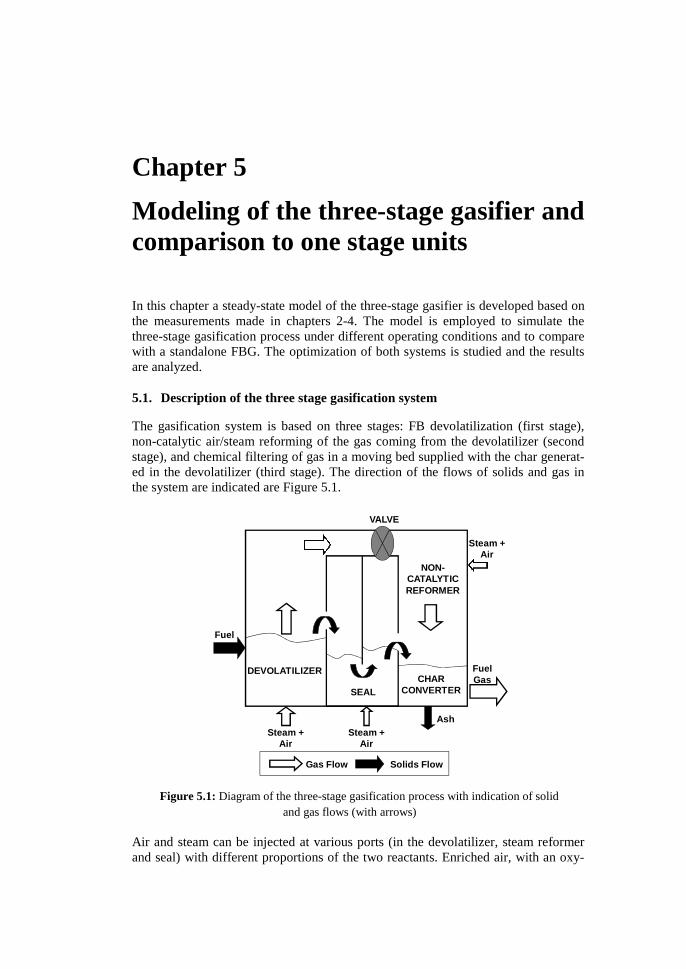
Chapter 5
Modeling of the three-stage gasifier and comparison to one stage units
In this chapter a steady-state model of the three-stage gasifier is developed based on the measurements made in chapters 2-4. The model is employed to simulate the three-stage gasification process under different operating conditions and to compare with a standalone FBG. The optimization of both systems is studied and the results are analyzed. 5.1. Description of the three stage gasification system
The gasification system is based on three stages: FB devolatilization (first stage), non-catalytic air/steam reforming of the gas coming from the devolatilizer (second stage), and chemical filtering of gas in a moving bed supplied with the char generat-ed in the devolatilizer (third stage). The direction of the flows of solids and gas in the system are indicated are Figure 5.1.
Figure 5.1: Diagram of the three-stage gasification process with indication of solid and gas flows (with arrows)
Air and steam can be injected at various ports (in the devolatilizer, steam reformer and seal) with different proportions of the two reactants. Enriched air, with an oxy-
DEVOLATILIZER
SEAL
VALVE
Gas Flow Solids Flow
CHAR CONVERTER
Fuel
Ash
Fuel Gas
NON-CATALYTICREFORMER
Steam + Air
Steam + Air
Steam + Air

90 Chapter 5
gen concentration of up to 40% (to keep the cost reasonably low, for instance, if produced by membranes) can be fed instead of air. The main processes occurring in each part of the system have been indicated in Figure 1.1. The devolatilizer is oper-ated at a relatively low temperature (700-750 °C) compared to one-stage gasification units. As a result, a high yield of tar is generated, this tar being more reactive (less aromatized) than that produced at high temperature in an atmosphere with a higher concentration of oxygen. The gas is homogeneously reformed and oxidized in the second stage, where a local temperature of up to 1200 °C is generated by the addi-tion of air or enriched air and steam. The injection of steam contributes to some extent to inhibit reactions of coking and polymerization (Hosokai et al., 2008). The gas is filtered in a moving bed made of char coming from the seal. In this stage, catalytic decomposition of tar on carbonaceous surfaces of the char takes place, while the char is gasified with steam and the gas is cooled down (chemical quench). As discussed previously the seal enables to separate the gas and solid flows coming from the devolatilizer. It can be operated as an oxidizer (fed with air or enriched air) or as a reformer (fed with H2O). The choice of operating mode depends on the fuel heating value and reactivity, ash properties and other conditions analyzed below. The system is designed to be autothermal and the air and steam fed to the system are preheated through heat exchange with the produced gas. The main considerations to take into account to predict the behaviour of the three-stage system become visible from the above description. It is necessary to character-ize: (i) For a given fuel, the effects of operating conditions in the devolatilizer on the yields of gas, char and tars, including the nature of the tar compounds in the gas; (ii) the mechanisms and rates of tar decomposition reactions under different operating conditions in the gas reformer and char filter (temperature, steam concentration and gas residence time); (iii) the rate of char gasification at a given temperature and gas composition; (iv) the fluid-dynamics of the system to characterize the solid and gas mixing in the devolatilizer and seal. The distribution of products during devolatiliza-tion has been studied in chapter 3, except for the characterization of tar, which has been studied elsewhere (Fuentes et al., 2011). The homogeneous and heterogeneous conversion of tar is not treated in this work, but is part of another thesis. Here these processes were modelled using a scheme of reaction that was assumed and kinetics data from literature, as will be discussed below during the model description. The experimental input and results obtained in chapters 2-4 that are employed in the model are listed below: From chapter 2:
• Minimum fluidization velocity • Method for calculating the bed porosity as a function of gas velocity • Perfect mixing of solids (RTD) • Equal distribution of the gas flow between the two chambers in the seal
From chapter 3:
• The devolatilization yields are not influenced by the composition of the flu-idizing gas, so distribution of products measured in N2 atmosphere can be employed.

Modeling of a three-stage gasifier 91
• Correlations for calculating product yields from devolatilization as a func-tion of temperature (Equation 3.8)
• Small overlapping in time between devolatilization and gasification of char (they can be modeled as processes occurring in series)
• Variations of size and shape of the DSS particles during devolatilization and combustion can be neglected.
• The devolatilization model developed enables calculation of devolatiliza-tion times for DSS of different particle sizes.
• Kinetics of the WGSR (it was concluded that the kinetics given by (Biba et al., 1978) can be employed).
From chapter 4:
• Kinetics of gasification of char from DSS, generated in situ in the bed, with CO2 and H2O (Equation 4.11)
• Competition between CO2 and H2O is not important, so the char conversion can be calculated using the sum of the individual reaction rates (Equation 4.12).
• Chemical kinetics of combustion of char from DSS (it was found that the kinetics given by (Dennis et al., 2005) can be employed)
5.2. Model development
A steady state model has been developed to simulate the conversion of DSS in the three-stage gasification system proposed. The DSS employed has been described in chapter 3. Firstly, a description is made of the relevant processes taking place in the gasifier, indicating the model details. Secondly, a reactor model integrating all these processes in Aspen is presented.
5.2.1. Modeling of relevant processes taking place in the gasifier
Devolatilization
The devolatilization of DSS was considered to yield the following species: CO, CO2, CH4, H2, light hydrocarbons, H2O, tars and char. Correlations for calculating the yields of CO, CO2, CH4, H2 and char as a function of temperature were employed (see chapter 3). Analysis of char (see Table 4.2) and tar (Fuentes et al., 2011) gener-ated during devolatilization in FB showed that the oxygen content was negligible. Therefore, all the oxygen contained in the DSS was assumed to form CO, CO2 and H2O and the yield of H2O was calculated from the oxygen balance. Toluene (C7H8) was employed to represent the tar produced during devolatilization. The yields of toluene and light hydrocarbons, represented by C2H6, were calculated to fulfill the carbon and hydrogen balances. The distribution of nitrogen containing compounds in the gas phase is not modeled, but assumed. The modeling of these compounds is out of the scope of the present model.
Combustion of char
The reaction of carbon with oxygen can yield both CO and CO2, but here it was assumed to yield only CO2 (R1), for simplicity. This is justified since the distribution

92 Chapter 5
between CO and CO2 during char combustion does not have a great influence on the results, because the CO/CO2 ratio in the gasifier is governed by the WGSR equilib-rium (Gómez-Barea and Leckner, 2010).
2 2+ →C O CO (R1)
It was observed in the laboratory tests that the DSS char particles maintain their size and shape during conversion (both for combustion and gasification) (see Figure 3.2), in agreement with previous work (Scott et al., 2007). Mass transfer limitations have shown to be important during combustion of DSS char in FB (Dennis et al., 2005). Then a shrinking unreacted core model (SUCM) was assumed, considering that the char particle size is equal to that of the fuel because the ash remains attached to the particle. The combustion reaction takes place on the outer surface of the unreacted core, whose position changes with time toward the centre of the particle, so the thickness of the ash layer increases with conversion. The chemical kinetics of the combustion of DSS from (Dennis et al., 2005) was employed, as discussed in chap-ter 4, with the additional simplification of first order reaction with respect to oxygen. Despite the experimental results suggesting that the reaction order is lower than one in the kinetic regime (n=0.75 in (Dennis et al., 2005) and n=0.88 in (Nowicki et al., 2010), the assumption of first-order kinetics simplifies the treatment and had very little impact on the results as confirmed by simulations. Taking into account the above considerations, the rate of char combustion rR1 per unit of particle volume was calculated using the following expression (Gómez-Barea and Leckner, 2010) for spherical particles:
21 1=R R Or k C (5.1)
1
1 2
6 1
1 1 1=
+ +
R
R
p p
g D iA c
kd d
k k k d
(5.2)
kD being a pseudo mass transfer coefficient of the ash layer defined as (Gómez-Barea et al., 2012b):
( )2
=−
e cD
p p c
D dk
d d d (5.3)
dc and dp being the diameter of the core and the char particle, respectively. kiAR1 is the kinetic coefficient based on the external surface. dc is calculated as a function of conversion, according to the SUCM (Gómez-Barea and Leckner, 2010):
( ) 131= −c p cd d x (5.4)
The particle size distribution of DSS was taken into account and a reaction rate was calculated for each particle size.
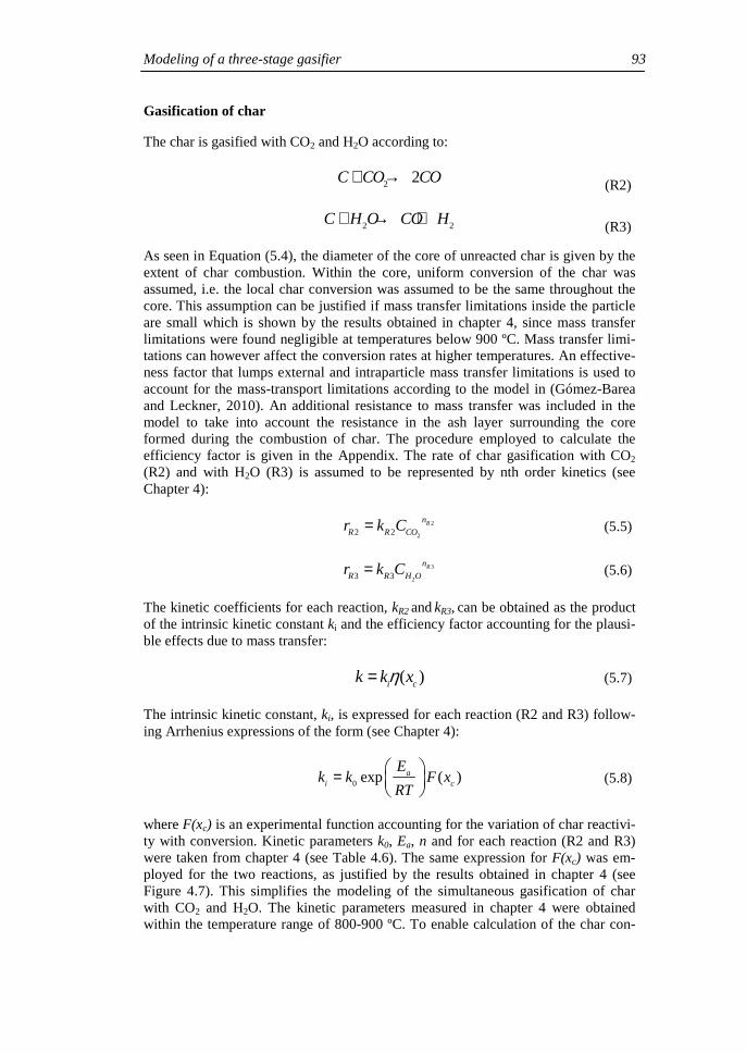
Modeling of a three-stage gasifier 93
Gasification of char
The char is gasified with CO2 and H2O according to:
2 2+ →C CO CO (R2)
2 2+ → +C H O CO H (R3)
As seen in Equation (5.4), the diameter of the core of unreacted char is given by the extent of char combustion. Within the core, uniform conversion of the char was assumed, i.e. the local char conversion was assumed to be the same throughout the core. This assumption can be justified if mass transfer limitations inside the particle are small which is shown by the results obtained in chapter 4, since mass transfer limitations were found negligible at temperatures below 900 ºC. Mass transfer limi-tations can however affect the conversion rates at higher temperatures. An effective-ness factor that lumps external and intraparticle mass transfer limitations is used to account for the mass-transport limitations according to the model in (Gómez-Barea and Leckner, 2010). An additional resistance to mass transfer was included in the model to take into account the resistance in the ash layer surrounding the core formed during the combustion of char. The procedure employed to calculate the efficiency factor is given in the Appendix. The rate of char gasification with CO2 (R2) and with H2O (R3) is assumed to be represented by nth order kinetics (see Chapter 4):
2
22 2= Rn
R R COr k C (5.5)
3
23 3= Rn
R R H Or k C (5.6)
The kinetic coefficients for each reaction, kR2 and kR3, can be obtained as the product of the intrinsic kinetic constant ki and the efficiency factor accounting for the plausi-ble effects due to mass transfer:
( )η= i ck k x (5.7)
The intrinsic kinetic constant, ki, is expressed for each reaction (R2 and R3) follow-ing Arrhenius expressions of the form (see Chapter 4):
0 exp ( )=
ai c
Ek k F x
RT (5.8)
where F(xc) is an experimental function accounting for the variation of char reactivi-ty with conversion. Kinetic parameters k0, Ea, n and for each reaction (R2 and R3) were taken from chapter 4 (see Table 4.6). The same expression for F(xc) was em-ployed for the two reactions, as justified by the results obtained in chapter 4 (see Figure 4.7). This simplifies the modeling of the simultaneous gasification of char with CO2 and H2O. The kinetic parameters measured in chapter 4 were obtained within the temperature range of 800-900 ºC. To enable calculation of the char con-

94 Chapter 5
version at temperatures below 800 ºC, additional tests have been carried out to de-termine the kinetics of the reaction with H2O below 800 ºC. The reaction rates below 800 ºC were fit empirically to be employed in the simulations in this temperature range. The effectiveness factor in Equation (5.7) was calculated separately for each reaction and for each particle size.
Kinetics of gas phase reactions
Gas phase reactions include the combustion of volatile species, water gas shift reac-tion (WGSR) and the conversion of tars. The volatiles combustion reactions and the WGSR are listed in Table 5.1 together with the kinetic expression employed for each reaction.
Table 5.1. Gas phase reactions: stoichiometry and kinetic expression taken from dif-ferent sources according to the screening made in (Gómez-Barea and Leckner, 2010).
Reaction Stoichiometry Kinetic expression Reference
R4 2 2 2
0.5 + →H O H O 2 24 4=R R H Or k C C Haslam, 1923
R5 2 2
0.5 + →CO O CO 2 2
0.5 0.5
5 5=R R CO O H Or k C C C Howard and Williams,
1973
R6 4 2 2
1.5 2+ → +CH O CO H O 4 2
0.7 0.86 6=R R CH Or k C C
Dryer and Glassman,
1973
R7 2 6 2 2 23.5 2 3+ → +C H O CO H O
2 6 2
0.1 1.65
7 7=R R C H Or k C C Westbrook and Dryer,
1981
R8 7 8 2 25.5 7 4+ → +C H O CO H O
7 8 2
0.5
8 8=R R C H Or k C C Bryden and Ragland,
1996
R9 2 2 2
+ ↔ +CO H O CO H
2
2 2
9 9,
9,
=
−R R d CO H O
R i CO H
r k C C
k C C
Biba et al., 1978; Yoon et
al., 1978
In Table 5.1 the oxidation of tar with O2 is included, however, cracking and reform-ing also occur, as well as interaction between different tar compounds. The kinetics of these reactions and the scheme of reaction has to be defined. The conversion of tar is a complex process involving a number of different species and reactions. Pri-mary tars, produced at relatively low temperature during the devolatilization, under-go thermal cracking inside the reactor yielding more stable tar species. At tempera-tures above 900 ºC tars are composed mainly of polyaromatic hydrocarbons (PAH) which are more stable and difficult to destroy (Gómez-Barea and Leckner, 2011). In order to convert these compounds into light fuel species without a catalyst, tempera-tures over 1100 ºC are required (Devi et al., 2002). As previously discussed (during description of the modeling of devolatilization), toluene (C7H8) was employed to represent the tar generated during devolatilization, here called light tar; naphthalene (C10H8) was taken as a representation of secondary tar, here called heavy tar. The homogeneous conversion of tar is modeled using two sequential reactions. In the first reaction, the light tar is cracked to give heavy tar and light gas (R10 in Table 5.2) and the second reaction involves the reforming of heavy tar into light gas and

Modeling of a three-stage gasifier 95
coke (R11 in Table 5.2). This reaction scheme was selected based on experimental findings in literature (discussed in chapter 1) that light tar is cracked to yield more heavy tar that can be converted to light gas compounds and coke when exposed to high temperatures. The kinetics given by (Jess, 1996) for the homogeneous conver-sion of toluene and naphthalene was used in the model, shown in Table 5.2. The stoichiometry of these reactions was not specified in literature (Jess, 1996), so com-patible stoichiometry was defined here. Since the amount of tar in the reactor is small compared to other gas species and char, the stoichiometry defined for the homogeneous conversion of tar (reactions R10 and R11) only has very small influ-ence on the results of temperature, gas composition and char conversion calculated by the model.
Table 5.2. Stoichiometry and kinetic expressions for the different tar reforming reac-tions considered
Reac-tion Stoichiometry Kinetic expression Refer-
ence
R10 7 8 2 10 8 4 2 63 3 6+ → + + +C H H C H CH C H C
7 8 2
0.5
10 10=R R C H Hr k C C
Jess, 1996
R11 210 8 4
2 3 2 5+ → + +C H H O CH CO C
10 8 2
1.6 0.5
11 11
−=R R C H Hr k C C
Jess, 1996
R12 10 8 2 2
10 10 14+ +→charC H H O CO H
10 812 12=R R C Hr k C
Abu El-Rub et
al., 2008
Reforming of tar catalyzed by the char
Reforming of heavy tar catalyzed by char particles (R12) may occur in the bed of char in the third stage of the process (char converter). Experiments for studying this reaction are currently ongoing, so in this model, the global stoichiometry shown in Table 5.2 and kinetics obtained for the reforming of naphthalene over wood char measured by (Abu El-Rub et al., 2008) were employed (see Table 5.2).
5.2.2. Reactor model
A reactor model of the three stage gasification system was developed taking into account the processes described above. The model can be divided into four submodels, representing the main parts of the system: fluidized bed devolatilizer (FBD), seal (LS), non-catalytic gas reformer (NCGR) and char converter (CR). Aspen Plus was taken as mother program to implement the submodels. A general scheme of the reactor model is shown in Figure 5.2. It includes the flows of solids and gas in the system as well as the processes involved in each part, indicating the reaction model subroutines used in Aspen. The system is assumed to be adiabatic and uniform (but different) temperature is considered for the FBD and the LS, as indicated in Figure 5.2. Since in a standalone FBG unit all the processes occur to-gether in a single vessel, the FBD submodel will be employed to simulate (i) the performance of the first stage of the three-stage FBG and (ii) the performance of a stand-alone FBG, allowing comparison between the three-stage system and a one-stage FBG.

96 Chapter 5
Figure 5.2: General scheme of the three-stage gasification model
The dimensions of the different vessels (FBD, LS, NCGR and CR) were defined as a function of the feedrate of DSS. The diameter of the FBD, LS and CR was specified using the throughput (kg DSS/h/m2). The throughput employed was 1700, 3800 and 430 for the FBD, LS and CR, respectively. These values were defined to adjust the gas velocity in each part. The dimensions of the NCGR were specified to have a gas residence time of 1.3 s. Simulations were carried out for a DSS flowrate of 30 kg/h, for which the vessel diameter was 15, 9 and 30 for the FBD, LS and CR, respective-ly. The gas in the bed was assumed to be well mixed and the bed porosity was calcu-lated according to the model presented in (Johnsson et al., 1991). The gas leaving the LS is divided into two streams with equal flowrates, resulting from the pressure balance of the system as discussed in chapter 2.
A detailed description of the submodels for the different parts of the system is given below. The acronyms employed (RYIELD, RPLUG and RSTOIC) are the names of the blocks available in Aspen to simulate reactors.
Fluidized-bed devolatilizer (FBD) submodel
In order to ensure complete devolatilization of the fuel a spatial time for the solids of 12 minutes and a minimum temperature of 750 ºC is considered for this unit. The temperature in the FBD is calculated and only simulations fulfilling the minimum temperature required are considered.
The drying and devolatilization of DSS, partial oxidation and gasification of char in the FBD were modeled as sequential steps as justified by experimental findings in chapter 3. The consumption of the oxygen fed is fast compared to char gasification
LSChar
GasAir Steam
Steam Gas
FBD
DSS
Air
Char
Gas
Devolatilization
RYIELD
Partial oxidation
RPLUGGas Char
Gasification of char
RSTOIC
Gas Char
WGSR/Tar reforming
RPLUG
Gas Char
TFBD
Char combustion/WGSRRPLUG
TLS
NCGRPartial oxidation /Tar
reforming /WGSRRPLUG
Air
CRGasification of char /Tar
reforming /WGSRRPLUG
Gas Gas
Steam

Modeling of a three-stage gasifier 97
so the partial oxidation can be considered to take place in a small part of the reactor, while char is gasified in most of the reactor volume.
The drying and devolatilization of DSS were simulated using an RYIELD unit and a calculator block, computing the yields of the different species during devolatilization as a function of the FBD temperature, applying the experimental correlations, as discussed in section 2.1.1.
In the partial oxidation step, the combustion of the volatiles and char generated dur-ing devolatilization is simulated (reactions R1, R4-R9). The combustion reactions are modeled using a plug flow reactor model (RPLUG). The char combustion rate constant, kR1, is calculated in an external calculator block, using Equations (5.2)-(5.4). kR1 decreases with char conversion due to the increase in the ash layer thick-ness around the reacting char particle, so the combustion process was simulated using a series of RPLUG units taking into account the effect of conversion.
The gasification of char was simulated using an RSTOIC unit with a calculator block that computes the conversion of the two char gasification reactions (R2 and R3). The char conversion, xc, attained in the FBD was calculated using the residence time distribution of solids obtained by assuming perfect mixing, given in Equation (2.23). This assumption is supported by results obtained in chapter 2 (see Figure 2.7). As discussed above, devolatilization and gasification of char were modeled as se-quential steps, so gasification was assumed to start once devolatilization was com-pleted. The time necessary for devolatilization of DSS was calculated for each parti-cle size using the model presented in chapter 3. The time needed to reach a certain char conversion was calculated using the sum of the gasification rates with CO2 and H2O as discussed in chapter 4:
0 2 3
1=
+∫cx
t c
R R
t C dxr r
(5.9)
The rates of the char gasification reactions, rR2 and rR3, are calculated according to Equations (5.5)-(5.8).
The WGSR (R9) and the tar conversion reactions are simulated using an RPLUG reactor. As can be seen in Figure 5.2, the gasification of char and the WGSR are modeled as sequential steps, but in a real gasifier they occur simultaneously. The effects of making this assumption on the results were found to be insignificant, so it is a reasonable simplification. As discussed above, the temperature was assumed to be uniform throughout the FBD and the reactor temperature was calculated by per-forming an energy balance by using the Aspen design specification tool.
Seal (LS) submodel
In the LS model, the combustion reactions (R1, R4-R8) and the WGSR (R9) are considered. The approach to modeling the combustion of char in the LS is the same as in the FBD: various RPLUG units in series were employed to account for the variations in xc. The temperature in the LS was calculated using the same method as for the FBD.

98 Chapter 5
Non-catalytic gas reformer (NCGR) submodel
The NCGR is simulated as an adiabatic plug flow reactor, using the RPLUG model, where the volatiles oxidation reactions (R4-R8), the WGSR (R9) and the homoge-neous reforming of tar (R10-R11) take place.
Char converter (CR) submodel
The CR is modeled as an adiabatic plug flow reactor. The reactions that are consid-ered to take place in the CR are: gasification of char (R2-R3), the WGSR (R9) and the homogeneous and heterogeneous reforming of tars (R10-R12). The rates of the char gasification reactions, rR2 and rR3, depend on the char conversion, and therefore, the CR was simulated using a series of RPLUG units. The number of units was suf-ficiently large to have negligible effect on the results. For each unit, F(xc), that gives the variation of the intrinsic kinetics with conversion (see Equation (5.8)) and the efficiency factor, η(xc), for each reaction, were calculated as a function of the char conversion, xc, in an external calculator block.
Inputs and outputs of the model
The inputs to the model are the flowrates of DSS, air and steam fed in the different parts of the system. Air and steam are assumed to be preheated up to 300 ºC, a value achievable by heat exchange with the exit gas. The outputs include temperatures, gas and char flows and gas composition in the different parts of the system. Various indexes are employed for the analysis of the results below, defined in the following:
• The equivalence ratio, ER, is the oxygen in the air fed divided by the oxygen necessary for complete oxidation of the fuel.
• The amount of steam fed to the system is characterized by the steam to oxygen mass ratio, SOR, in kg steam/kg of oxygen.
• The carbon conversion efficiency, CC, is the mass of carbon in the produced gas (including tars) divided by the amount of carbon fed with the DSS.
• The cold gas efficiency, CGE, is the chemical energy of the gas repre-sented by the higher heating value in the produced gas, divided by the higher heating value in the DSS fed. The energy in the tars has been included as part of the chemical energy in the gas, despite it is obvious that condensable tars will not be present in a cold gas.
=ɺ
ɺ
out out
in in
g g
DSS DSS
m HHVCGE
m HHV (5.10)
5.3. Results and discussion
In the first part of this section, the FBD submodel is employed to simulate the per-formance of a stand-alone FBG. Thereafter, the simulation of the three-stage gasifi-cation system is made, focusing on a comparison between one-stage and three-stage gasification systems. Optimization of the operating conditions of a three-stage gasifier is analyzed and then finally gasification using enriched air is studied.
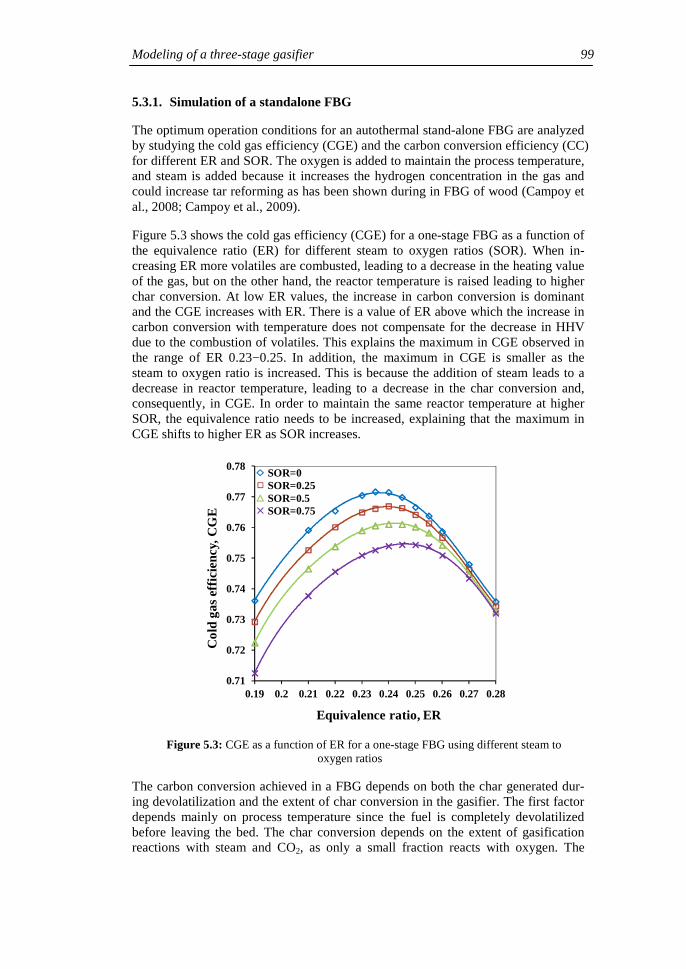
Modeling of a three-stage gasifier 99
5.3.1. Simulation of a standalone FBG
The optimum operation conditions for an autothermal stand-alone FBG are analyzed by studying the cold gas efficiency (CGE) and the carbon conversion efficiency (CC) for different ER and SOR. The oxygen is added to maintain the process temperature, and steam is added because it increases the hydrogen concentration in the gas and could increase tar reforming as has been shown during in FBG of wood (Campoy et al., 2008; Campoy et al., 2009).
Figure 5.3 shows the cold gas efficiency (CGE) for a one-stage FBG as a function of the equivalence ratio (ER) for different steam to oxygen ratios (SOR). When in-creasing ER more volatiles are combusted, leading to a decrease in the heating value of the gas, but on the other hand, the reactor temperature is raised leading to higher char conversion. At low ER values, the increase in carbon conversion is dominant and the CGE increases with ER. There is a value of ER above which the increase in carbon conversion with temperature does not compensate for the decrease in HHV due to the combustion of volatiles. This explains the maximum in CGE observed in the range of ER 0.23−0.25. In addition, the maximum in CGE is smaller as the steam to oxygen ratio is increased. This is because the addition of steam leads to a decrease in reactor temperature, leading to a decrease in the char conversion and, consequently, in CGE. In order to maintain the same reactor temperature at higher SOR, the equivalence ratio needs to be increased, explaining that the maximum in CGE shifts to higher ER as SOR increases.
Figure 5.3: CGE as a function of ER for a one-stage FBG using different steam to oxygen ratios
The carbon conversion achieved in a FBG depends on both the char generated dur-ing devolatilization and the extent of char conversion in the gasifier. The first factor depends mainly on process temperature since the fuel is completely devolatilized before leaving the bed. The char conversion depends on the extent of gasification reactions with steam and CO2, as only a small fraction reacts with oxygen. The
0.71
0.72
0.73
0.74
0.75
0.76
0.77
0.78
0.19 0.2 0.21 0.22 0.23 0.24 0.25 0.26 0.27 0.28
Co
ld g
as e
ffici
ency
, CG
E
Equivalence ratio, ER
SOR=0SOR=0.25SOR=0.5SOR=0.75

100 Chapter 5
amount of char gasified is determined mainly by the temperature and residence time of the char in the bed, the gas composition having only a minor influence, as demon-strated in Figure 5.4. In this figure, the carbon conversion efficiency is represented as a function of the reactor temperature for different steam to oxygen ratios, showing that nearly equal carbon conversion is attained in simulations with the same temper-ature but different SOR (different steam concentration in the gasifier). It can also be seen that the char conversion increases steeply with increasing temperature up to 900 ºC, while after that, the increase levels off. Calculations show that for all the steam to oxygen ratios analyzed, the maximum CGE occurs for a reactor tempera-ture between 880 and 890 ºC, corresponding to an ER ranging between 0.23 and 0.25 (see Figure 5.3).
Figure 5.4: Carbon conversion (CC) achieved in a one-stage FBG as a function of re-actor temperature for different steam to oxygen ratios (SOR)
The addition of steam also influences the composition of the produced gas. For ER=0.24 and SOR varying between 0 and 0.25, the CO molar fraction in the dry gas is lowered from 13.5% to 11.6%, whilst the H2 and CO2 molar fractions increase, respectively, from 8.0 to 9.1% and from 14.9 to 16.3%. These effects are explained by the enhancement of the WGSR for higher steam concentrations, leading to the formation of H2 and CO2.
The tar content in the produced gas depends on the tar yield during devolatilization and the extent of oxidation and reforming of tar. Since the addition of steam increas-es the H2 concentration, it could enhance the reforming of light tar inside the reactor (see reaction R10). Simulations have been carried out for different equivalence rati-os using SOR=0 and SOR=0.25 to study the influence on the tar content in the pro-duced gas. The results are shown in Figure 5.5, where the tar content in the gas (g/Nm3
dry gas) and the conversion of light tar due to reforming (reaction R10), xR10 (in %) are represented on the left side vertical axis. The reactor temperature is also shown and can be read on the right side vertical axis. The results show that the re-forming of tar in the gasifier is not significant for temperatures below 900 ºC (xR10 is
0.82
0.84
0.86
0.88
0.9
0.92
0.94
0.96
0.98
1
750 800 850 900 950 1000 1050
Ca
rbo
n co
nver
sion
, C
C
Temperature, ºC
SOR=0SOR=0.25SOR=0.5SOR=0.75

Modeling of a three-stage gasifier 101
about 10% at 900 ºC). When increasing the steam to oxygen ratio the temperature decreases, leading to less reforming of tar and higher tar content in the gas. These results suggest that the addition of steam is not suitable to enhance tar reforming for atmospheric autothermal FBG. Nonetheless, the values calculated should be consid-ered with caution since the effect of steam on the rate of conversion of tar com-pounds is not well known. We have modeled the process with kinetics currently available in the literature. However, there are other factors in a FBG that may influ-ence the tar yield such as the generation of plumes of volatiles in the feed ports, the heterogeneous conversion of tar with the bed material and others that have not been taken into account in the model developed. Further studies are necessary to quantify steam reforming of tars under different FBG conditions. In spite of this, the model results are useful to predict the temperature because the influence of the extent of tar conversion on the thermal balance is small, so the model is reliable in the analysis of the effects of ER and SOR on CGE and CC.
Figure 5.5: Tar content in the gas produced in a one-stage FBG (including both light and heavy tar) and the conversion of light tar due to reaction R10, xR10, represented on the left side vertical axis, and reactor temperature represented on the right side vertical axis, as a
function of equivalence ratio, for SOR=0 (solid lines) and SOR=0.25 (dashed lines)
The operating conditions that give the maximum efficiency for a one-stage FBG were identified as ER=0.236 and SOR=0. Figure 5.6(a) shows the main results ob-tained for that case, including reactor temperature, CGE, CC and the tar content in the gas. Practical operating experience using DSS in an FBG has shown that defluidization problems due to partial sintering of the DSS with bed material starts occurring from temperatures above 810-820 ºC (Gómez-Barea et al., 2008). There-fore, a FBG using DSS cannot be operated at temperatures above this value and the maximum CGE that can be achieved is lower than the one shown in Figure 5.6(a). A simulation was performed to determine the maximum CGE that can be achieved in a standalone FBG using ER=0.207 and SOR=0, which gives a reactor temperature close to 820 ºC. The results from this simulation are shown in Figure 5.6(b). The loss of performance for this reactor temperature is visible, yielding a CGE of 0.75 and tar content in the gas of 31 g/Nm3
dry gas.
Tar content
xR10
T
750
775
800
825
850
875
900
0
10
20
30
40
50
60
0.16 0.18 0.2 0.22 0.24
Tem
pera
ture
, ºC
Tar c
onte
nt (
light
+he
avy)
, g/N
m3
Con
vers
ion
of li
ght t
ar (
x R10
), %
Equivalence ratio, ER

102 Chapter 5
Figure 5.6: Simulation of a one-stage FBG, using (a) ER=0.236 and SOR=0 (Simula-tion 1.1) to give the maximum CGE; (b) ER=0.207 and SOR=0 (Simulation 1.2) to give the maximum operating temperature and simulation of a three-stage system using total
ER=0.240 and total SOR=0.28 (c) (simulation 3.1) (see Table 5.3)
5.3.2. Simulation of a three-stage FBG
In the three-stage gasifier, the air fed is divided between the FBD, LS and NCGR. A maximum temperature of 820 ºC is set for the seal and therefore only a small flow of air can be fed in this part and the addition of steam is necessary to fluidize the seal. This leads to a minimum requirement of steam given by SOR ranging from 0.20 and 0.30. Since part of the steam fed in the seal is directed to the gas reformer (see Fig-ure 5.2) and we have no accurate knowledge about how much steam should be add-ed in the gas reformer, no steam will be fed to the system apart from the steam fed in the LS. A simulation of the three-stage system has been performed using a total ER of 0.24, a value close to the optimum for a one-stage FBG when SOR is between 0.20 and 0.30 and the results are shown in Figure 5.6(c). Comparing the results in Figure 5.6, it can be concluded that a significant improvement is achieved by using the three-stage gasifier. The higher cold gas efficiency achieved is explained by the higher char conversion obtained by increasing the char residence time in the system using a moving bed of char (CR). In a one-stage FBG most of the oxygen combines with fuel volatiles and only a limited part burns the char. Therefore, the char conver-sion in a one-stage FBG has to be achieved by gasification with CO2 and H2O, which are not fast enough to convert the char within the time of stay of the char particles in the reactor. Compared to the one-stage FBG, the exit temperature in the three-stage system is lower, due to the endothermic reactions taking place in the CR, decreasing the heat loss in the system. The char gasification and tar cracking reac-tions taking place in the CR also increase the CO and H2 content of the gas raising its heating value. Despite the increase in gasification efficiency achieved in the
Fuel
ProducedGas
Air
T = 822 ºC
CGE: 0.82 CC: 0.97
Tar: 4.3 g/Nm3dry gas
One stage, Sim 1.2
Fuel
ProducedGas
Air
T = 888 ºC
CGE: 0.77 CC: 0.94
Tar: 19 g/Nm3dry gas
Input: ER: 0.236SOR: 0
One stage, Sim 1.1
(a) (b)
Fuel
Producedgas
Air
Solids out
SteamAir
Air
T = 810 ºC
Tmax = 995 ºC
T = 662 ºC
Three stages, Sim 3.1
(c)
CGE: 0.75 CC: 0.89
Tar: 31 g/Nm3dry gas
Tin = 956 ºC
Tout = 821 ºC
Input: ER: 0.207SOR: 0
Input: ER: 0.240SOR: 0.273
Results: Results: Results:

Modeling of a three-stage gasifier 103
three-stage system, the tar content in the produced gas shown in Figure 5.6 (c) is still high and needs to be decreased further.
In order to enhance the conversion of tar in the system it is necessary to create a high temperature zone in the NCGR with peak temperatures around 1200 ºC (in simula-tion 3.1 shown in Figure 5.6(c) the maximum temperature in the NCGR was below 1000 ºC). For this purpose, the total ER in the system needs to be increased. Differ-ent distributions of the air fed between the FBD and the gas reformer can be chosen. Two simulations were performed giving a temperature peak in the NCGR of 1200 ºC, by adjusting the air flow in this part. In the first simulation (simulation 3.2), the air flow in the FBD was adjusted so that a temperature of 750 ºC was reached in this section (the minimum set) and in the second simulation (simulation 3.3) the temper-ature in the FBD was kept at its maximum (about 820 ºC). The details of the input values and results from the two simulations are given in Table 5.3.
Table 5.3. Distribution of air into the different parts of the three-stage gasifier, and the results obtained for two simulations (3.2 and 3.3), where the peak temperature in the
NCGR is 1200 ºC, but different distributions of air between the FBD and NCGR are em-ployed.
Simulation Total ER and SOR and air distribution
Total ER
Air fraction into FBD
Air fraction into LS
Air fraction into NCGR
Total SOR
3.2 0.270 0.62 0 0.38 0.24
3.3 0.298 0.70 0 0.30 0.22
Simulation
Results
TFBD, ºC
TLS, ºC
Tmax
NCGR,ºC Texit CR,
ºC CGE CC
Tar content, g/Nm3
dry
gas
HHV, MJ/Nm3
dry
gas
3.2 750 597 1201 888 0.81 0.993 0.01 6.9
3.3 822 677 1201 1012 0.76 1 0 6.4
As can be seen, the CGE is lower for simulation 3.3. This is because the total ER is higher in this case, while only a small increase in CC is achieved compared to simu-lation 3.2. For simulation 3.2 the CC is nearly complete, showing that there is little opportunity for improvement by increasing ER. The difference in efficiency between the two cases is also evidenced by the difference in exit temperature. For simulation 3.3 an important amount of energy is lost as sensible heat of the gas and ashes leav-ing the system. For both simulations the tar content in the exit gas was low, showing a substantial improvement compared to the results shown in Figure 5.6(c) (simula-tion 3.1). Figure 5.7 shows the tar content (both light and heavy tars) in the gas at the exit of the FBD, NCGR and CR, for simulations 3.1 and 3.2. For simulation 3.1 part of the light tar formed in the FBD is converted in the gas reformer leading to an increase in the heavy tar content. There is no significant reduction of light tar in the char converter, because the temperature in this section is not high enough. Heavy tar, on the other hand, is reduced through heterogeneous conversion catalyzed by the char particles. For simulation 3.2, the light tar content at the exit of the FBD is very high, but due to the high temperature in the NCGR all the light tar is reformed (Fig-

104 Chapter 5
ure 5.7 shows zero light tar at the exit of the NCGR), yielding heavy tar which is subsequently converted in the gas reformer and in the CR. For this simulation, the tar content at the exit of the CR is so low that it is not observed in Figure 5.7.
Figure 5.7: Light and heavy tar content of the gas at the exit of the devolatilizer (FBD), gas reformer (NCGR) and char converter (CR) for simulation 3.1 (see Figure 5.5(c)) and
simulation 3.2 (see Table 5.3).
To understand the conversion process in the char converter, Figure 5.8 represents the profiles of temperature and conversion of char and light- and heavy tar in this equipment for simulations 3.1 (Figure 5.8(a)) and 3.2 (Figure 5.8(b)). For simulation 3.2 no light tar is present in the CR (see Figure 5.7). It can be seen that the conver-sion of heavy tar and char are fast in the first section of the char converter, where the temperature is high, decreasing continuously due to the temperature drop along the reactor. In contrast, the conversion of light tar is seen to be slow throughout the whole unit (see Figure 5.8(a)). As can be seen in Figure 5.8 the simulations were carried out using a length of the CR equal to 1 m, but for simulation 3.2 (see Figure 5.8(b)) for reactor lengths higher than 0.5 m the rates of conversion of tar and char become very slow, as the degree of conversion is high and the temperature is low, so little benefit is achieved by increasing the length of the char converter above 0.5 m. It is obvious from Figure 5.8 that the length of the CR required depends on the oper-ating conditions. It can also be seen that very high temperatures are present in the first part of the CR. At these high temperatures mass transfer limitations within the particle can be important for the gasification of char. However, the model employed here to account for mass transfer limitations is still valid, because the minimum η value calculated (see Appendix) is close to 0.5.
Exit FBD
Sim 3.2 Sim 3.1
Exit CR
Sim 3.1
Exit NCGR
Sim 3.2 Sim 3.1Sim 3.20
10
20
30
40
50
60
Tar c
onte
nt,
g/N
m3
dry
gas
Light tar
Heavy tar
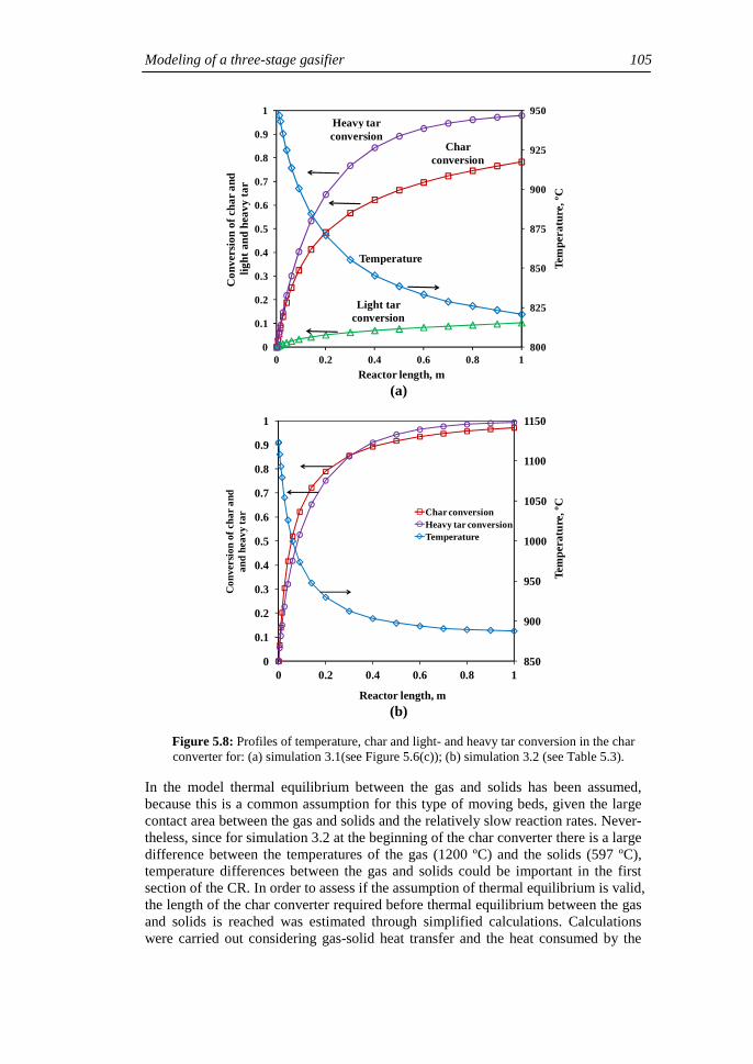
Modeling of a three-stage gasifier 105
(a)
(b)
Figure 5.8: Profiles of temperature, char and light- and heavy tar conversion in the char converter for: (a) simulation 3.1(see Figure 5.6(c)); (b) simulation 3.2 (see Table 5.3).
In the model thermal equilibrium between the gas and solids has been assumed, because this is a common assumption for this type of moving beds, given the large contact area between the gas and solids and the relatively slow reaction rates. Never-theless, since for simulation 3.2 at the beginning of the char converter there is a large difference between the temperatures of the gas (1200 ºC) and the solids (597 ºC), temperature differences between the gas and solids could be important in the first section of the CR. In order to assess if the assumption of thermal equilibrium is valid, the length of the char converter required before thermal equilibrium between the gas and solids is reached was estimated through simplified calculations. Calculations were carried out considering gas-solid heat transfer and the heat consumed by the
Char conversion
Light tar conversion
Heavy tar conversion
Temperature
800
825
850
875
900
925
950
0
0.1
0.2
0.3
0.4
0.5
0.6
0.7
0.8
0.9
1
0 0.2 0.4 0.6 0.8 1
Tem
pera
ture
, ºC
Co
nver
sion
of c
har a
ndlig
ht a
nd h
eavy
tar
Reactor length, m
850
900
950
1000
1050
1100
1150
0
0.1
0.2
0.3
0.4
0.5
0.6
0.7
0.8
0.9
1
0 0.2 0.4 0.6 0.8 1
Tem
pera
ture
, ºC
Co
nver
sion
of c
har a
ndan
d he
avy
tar
Reactor length, m
Char conversionHeavy tar conversionTemperature

106 Chapter 5
char gasification reactions. A heat transfer coefficient between the gas and solid of 100 J/(m2 s) was assumed, which is a conservative value compared to values ob-tained from correlations found in literature, that give h≈200 J/(m2 s) (Wakao and Kaguei, 1982). The results of the calculations showed that after less than 1 cm of reactor the temperature difference between the gas and solids is 1 ºC, so it can be concluded that the assumption of thermal equilibrium between the two phases is valid. 5.3.3. Simulation of a three-stage FBG with enriched air
A number of simulations were performed in order to check if the results obtained for the three-stage system can be improved by using enriched air, with an oxygen con-tent of 40% on a volume basis, as a gasification agent instead of air. The results show that with enriched air a peak temperature in the NCGR of 1200 ºC can be achieved using a total ER of 0.24 (simulation 3.4). This value can be compared to ER=0.27 needed when using air (see simulation 3.2). With enriched air, a CGE of almost 0.85 was achieved and the HHV of the gas was 10.8 MJ/Nm3
dry gas (compared
to the HHV of 6.9 MJ/Nm3 dry gas obtained with air in Simulation 3.2, see Table 5.3). The advantages of using enriched air can be explained by the fact that for the same equivalence ratio, less N2 is fed, which leads to a higher temperature in the system and less dilution of the gas, increasing the rates of char and tar conversion reactions and increasing the HHV of the gas. In Table 5.4, the composition of light gas com-ponents in the exit gas for the different simulations presented above is given. The results show that for the three-stage system, the CO and H2 contents in the gas in-crease compared to a one-stage FBG, while the CO2 decreases (note that the volume fraction of CO2 in Table 5.4 is higher for the enriched-air case since less gas is pro-duced, but the yield of CO2 in gCO2/kgdry fuel is lower). A comparison between simula-tions 3.1 and 3.2 shows that by optimizing the operating conditions for the three stage system, the CO and H2 content in the gas can be increased further at the ex-pense of the CO2. This can be explained by the char gasification and tar reforming reactions taking place. Finally, the concentration of all the gas compounds other than N2 increases by using enriched air, since the gas is less diluted with N2. It is shown that a gas with a concentration of CO and H2 of, respectively, 23.5% and 15.4% can be produced.
Table 5.4. Composition of the light gas obtained in different simulations, given in volume%dry gas
Composition of the dry gas, volume%
Simulation N2 CO CO2 CH4 H2 C2H6 One stage; simulation 1.1 52.3 13.4 15.1 4.2 7.3 2.6
One stage; simulation 1.2 50.9 11.7 16.4 4.3 8.9 3.2
Three stages; simulation 3.1
49.3 14.1 14.9 3.8 10.2 2.7
Three stages; simulation 3.2
51.3 15.3 13.7 3.6 10.6 2.2
Three stages; simulation 3.3
55.1 13.2 14.7 3.8 7.8 2.3
Three stages, enriched air; simulation 3.4
27.8 23.5 18.7 6.1 15.4 3.7

Modeling of a three-stage gasifier 107
5.4. Conclusions
A model of a new three-stage gasification system has been developed. The system is composed of a fluidized-bed devolatilizer (first stage), a non-catalytic gas reformer (second stage) and the third stage, called char converter, is a moving bed made up of particles coming from the first stage. The model has been used to compare the per-formance of the three-stage system and a stand-alone fluidized-bed gasifier (FBG) using dried sewage sludge (DSS) as fuel. The inputs from the model have been ob-tained in chapters 2-4. In the one-stage FBG, the operating temperature is limited to 810-820 ºC due to the risk of defluidization caused by sintering of the DSS ash. These temperatures are too low to enable conversion of tars, so a gas with high tar content (31 g/Nm3dry gas) is produced. In an autothermal three-stage FBG it is possi-ble to create distinct temperature zones by adjusting the operating conditions. The conversion of tar is favored by creating a high temperature zone in the non-catalytic gas reformer, where most tar coming from the first stage is converted into light gas components and heavy tar. The heavy tar can be converted in the moving bed of char due to the catalytic activity of the char particles, so that a gas with a tar content as low as 0.01 g/Nm3dry gas can be produced. The gasification of char is increased in the char converter due to the high solids residence time and high temperatures in this unit. The temperature is high at the beginning of the char converter, but continuously decreases due to the endothermic tar and char conversion reactions taking place. The rate of these reactions becomes slow towards the end of this unit as the temperature is low and the conversion of tar and char is high. The length of the char converter necessary to reach high conversion of char and tar depends on the operating condi-tions in the system. The best results for the three-stage gasifier are achieved when just enough air is fed to the system to assure devolatilization of the fuel in the first stage (temperature of 750 ºC) and a high temperature zone (1200 ºC) in the gas re-former. In this case the cold gas efficiency is 0.81, the HHV of the gas is 6.9 MJ/Nm3
dry and almost complete conversion of char is achieved. The heavy tar con-tent is virtually converted in the system, leading to a gas with a low enough dew point for burning in a gas engine. Using enriched air with a 40% volume of oxygen instead of air, the cold gas efficiency can be increased up to almost 0.85 and a gas with a HHV of 10.8 MJ/Nm3
dry gas can be achieved. In a future work the inhibition effect of H2 on the char gasification reaction with steam will be assessed. This effect leads to even lower char conversion in a standalone FBD, given the low operating temperatures, but in the three-stage system the temperature and char residence time are sufficiently high to achieve high char conversion. Due to the low tar content in the gas, the high efficiency of the process, and the advantages of the FB design, the proposed three-stage system is ideal for power production at small-to-medium scale, enabling high throughput as well as adaption to a variety of fuel size and quality (biomass, residues and wastes). The model developed in the present work has been employed to design a pilot plant for the demonstration of the system.

108 Chapter 5
Appendix: Model for the calculation of the effectiveness factor employed in Equation (5.7)
The global effectiveness factor is calculated as the product of the external and inter-nal effectiveness factors, ηe and ηi.
η η η= e i (5.11)
ηe and ηi are calculated by iteration using the following equations:
( ),1η η η= −n
e ch e i eDa (5.12)
( )11/22
,
11/22
,
tanh ηη
η
−
−=
nn
e ch i
i nn
e ch i
Da
Da (5.13)
Dach,e and Dach,i are non-dimensional parameters that are calculated from Equations (5.14) and (5.15), respectively.
2 2
1
, /
1 1
6−= +
p n
ch e i H O CO
g D
dDa k C
k k (5.14)
2 1
,
1
36 2
−+=
n
c ich i
e
d k CnDa
D (5.15)
In Equation (5.14) the term 1/kD has been added in order to account for the mass transfer resistance in the ash layer. kD and dc are calculated from Equations (5.3) and (5.4), respectively.

Chapter 6
Conclusions
6.1. Aim and significance
Gasification of waste fuels in conventional fluidized bed gasifiers (FBGs) presents high tar content in the gas and low carbon conversion, the latter due to incomplete conversion of char. In order to overcome these drawbacks alternative gasifier designs are needed, particularly for small-to-medium scale systems where extensive second-ary gas cleaning is not economically feasible. For this purpose, a new three-stage gasification system based on fluidized bed (FB) design has been developed.
The aim of this work is to assess the performance of the proposed three-stage gasifi-cation system. To achieve this goal a model was developed using dried sewage sludge (DSS) as reference fuel. DSS is available in large quantity, presenting a disposal prob-lem. Distributed-electricity production from this waste seems to be feasible.
Experimental data needed for the modeling of the system were obtained. Distribution of product species from devolatilization and the rate of char conversion were meas-ured in a laboratory FB. The fluid-dynamics of the system were investigated in a cold model, where the mixing of solids and gas in the system was characterized and corre-lations for calculating the key fluid-dynamics parameters to be used in the simulation model were obtained.
Simulations showed that the three-stage system significantly improves the perfor-mance of conventional FBG (one-stage system). Therefore the proposed new gasifier is an interesting technology for electricity production from biomass and waste.
6.2. List of contributions
Fluid-dynamics of the system
1. Minimum fluidization velocities, umf, of different materials were measured, includ-ing mixtures of DSS and inert bed material. Proper methods and correlations from literature were selected enabling calculation of the umf with good agreement with experimental measurements made in the cold model. 2. The distribution of solids in the bed for different solids mixtures under various gas velocities was measured. Correlations from literature enabling calculation of suspen-sion density in the bed, with good agreement with experimental measurements, were selected.

110 Chapter 6
3. Residence time distribution of the solids in the FB was measured showing that perfect mixing of the solids can be assumed. 4. The distribution of gas and solids in the seal (a FB divided into two parts by a sepa-ration wall covering part of the bed) was investigated, finding that the gas flow is divided equally between the two chambers in the seal for all operating conditions tested. Devolatilization
5. Product yields and devolatilization times were measured for different biomass and waste fuels in a laboratory fluidized bed at temperatures between 750 and 900 ºC. Correlations for the product yields as a function of temperature were obtained. 6. The shrinking and fragmentation behavior during devolatilization and char combus-tion was studied for different fuels. For DSS the variations in particle size and shape were small. 7. A simple model that can be employed to characterize the mode of conversion of a fuel particle was developed allowing estimation of the devolatilization time for differ-ent particle sizes. 8. Overlapping in time between devolatilization and gasification of char was found to be small, indicating that the two processes can be modeled as sequential processes (in series). 9. The influence of the composition of the fluidizing gas on the distribution of prod-ucts during devolatilization was found to be small. Therefore, the yields obtained using nitrogen can be assumed valid under gasification conditions, where a complex gas mixture surrounds the particle during devolatilization. 10. Kinetics of the WGSR was obtained in the laboratory reactor. The values of kinet-ics parameters measured were of the same order of magnitude (but lower) compared with kinetics commonly used in literature for gasification modeling. Conversion of char
11. Cooling of char after generation was found to influence the char reactivity signifi-cantly. Therefore char kinetics should be measured by in situ tests (those measuring the reactivity just after devolatilization, i.e. without intermediate cooling). 12. Kinetics of the gasification of char from dried sewage sludge (generated in situ in the laboratory fluidized bed) with CO2 and H2O was obtained. 13. The reactivity of char in mixtures containing CO2 and H2O simultaneously was investigated. It was demonstrated that competition between CO2 and H2O during gasification of dried sewage sludge char at atmospheric pressure is not important, meaning that the rate of char gasification can be calculated as the sum of the individu-al reaction rates obtained using mixtures of CO2‒N2 and H2O‒N2.

Conclusions 111
14. Rates of combustion of char from dried sewage sludge in air were measured. It was concluded that mass transfer limitations are important at practical temperature in a FBG in agreement with previous work in literature. The char combustion rate meas-ured at low temperature also showed reasonable agreement with kinetics from litera-ture. Modeling of the three-stage gasification system
15. A reactor model for simulation of the three stage gasification system was devel-oped using the experimental data and conclusions obtained in previous experimental studies (items 1-14). 16. The model was employed first to simulate the performance of a conventional standalone FBG for comparison with the three-stage system. For a standalone FBG the operating temperature is limited due to the risk of sintering of the ash, so the best results that could be obtained were: a cold gas efficiency of 0.75 and tar content in the gas of over 30 g/Nm3dry gas. 17. The model was employed to study the performance of the three-stage gasifier. It was found that the operation with air can be optimized to achieve a cold gas efficien-cy of 0.81, producing a gas with sufficiently low tar content (0.01 g/Nm3dry gas) to be employed for electricity production in engines. A process efficiency of up to 0.85 and a gas, virtually free of tars, with a higher heating value of 10.8 MJ/Nm3dry gas can be obtained using enriched air, with 40% volume of oxygen. Although the reported fig-ures are subjected to the assumptions and kinetics employed in the model, the results clearly indicate that the efficiency and quality of the gas obtained in standalone FB gasifier are insufficient, while the three-stage gasifier can produce a gas with the desired quality and with high process efficiency. 18. Besides the specific results present in this thesis, the methodology to obtain the necessary experimental data for any biomass species has been defined. The model of the three-stage gasification system developed can, therefore, be adapted to simulate the conversion of other biomass and waste fuels.
6.3. Future work
In this work various submodels and assumptions have been made. Some of them need further research. The main effort to improve the model should be focused on the fol-lowing: • Tar model: A simple reaction model based on experimental observations from
literature was developed for simulating the conversion of tar. A more detailed model of the conversion of tar is required. For this purpose data regarding the primary generation and kinetics of secondary conversion of a complex (real) mix-ture of tars are required. The kinetics data of the conversion of tar should be ob-tained both for homogeneous conditions using different gas compositions and for heterogeneous conversion catalyzed by char particles. These data could be in-cluded in the model in order to perform more accurate simulations of the conver-sion of tar in the system. Currently tar kinetics are being determined in another thesis.

112 Chapter 6
• Char model: A more detailed model representing the char converter (moving bed) could be developed, using the tar conversion data mentioned above and a more detailed particle model, for simulating the simultaneous conversion of char and tar. In addition, the inhibition effects of H2 during gasification of char should be taken into account in the kinetics.
• Kinetics of the WGSR in the presence of different inert or catalyst bed materials,
biomass species and char should be measured to explore future optimization of the system.
In addition, data from a pilot plant of the three-stage gasifier should be compared with the simulation results, in this way, both model and pilot plant can be improved and optimization for other fuels can be made. The pilot plant has been designed using the present model. The engineering work on the plant is currently ongoing.

Nomenclature
A Pre-exponential factor, s-1
Ar Archimedes number, -
Ari Archimedes number of inert particle (i), gdi3ρg (ρp-
ρg)/µg2
a, b, c Fitting parameters in Equation (4.9), -
a0, a1, a2 Coefficients of Eq. (2)
Bi Biot number, hR/λeff
b Geometry factor (in chapter 3)
C Gas concentration, mol/m3
C1, C2 Empirical parameters in Equation (2.5)
Ct Total gas concentration, mol/m3
CC Carbon conversion efficiency, -
CGE Cold gas efficiency, - (defined in Equation (5.10))
cp Specific heat capacity, J/(kg K)
Dach,e External mass Damköhler number for char conversion, -
Dach,i Internal mass Damköhler number for char conversion, -
Dadev Dahmköhler number, kdevρpcp,pR2/λeff
De Effective diffusivity, m2/s
d Particle diameter, m
db Bubble diameter, m
dc Diameter of the core containing unconverted char, m
deq Equivalent diameter, (6Vp/π)1/3, m
dp Particle diameter, m
Ea Activation energy, J/mol
ER Equivalence ratio
Fo Fourier number, λeff t/(ρpcp,pR2)

114 Nomenclature
F(xc) Function that expresses the variation of gasification rate
with char conversion, -
Fs Solids feed rate, kg/s
H Height of the vessel, m
HHV Higher heating value, J/kg
H Height of the bed, m (in chapter 2)
H Heat transfer coefficient, W m-2 (in chapter 3)
hgap Height of the opening below the separation wall, m
K Equilibrium constant of the WGSR, -
K Kinetic constant, s-1 (in chapter 3)
K Rate constant, (mol/m3)1-n s-1 (in chapter 5)
k0 Preexponential factor, bar-ns-1 (in chapter 4)
k0 Preexponential factor, (mol/m3)1-n s-1 (in chapter 5)
kd Kinetic constant of the direct WGSR, m3/(mol s)
kD Mass transfer coefficient for the ash layer, m s-1
kg Gas phase mass transfer coefficient, m s-1
ki Kinetic constant of the inverse WGSR, m3/(mol s) (in
chapter 3)
ki Intrinsic volumetric rate constant, (mol/m3)1-n s-1 (in
chapter 5)
kiA Kinetic constant referred to the external particle surface
area, m s-1
L Width of the vessel, m
mt Mass of painted DSS in the bed, kg
ṁ Mass flow, kg/s
m(t) Mass of C, H and O in the sample at time t, g
m0 Initial mass of painted DSS in the bed, kg (in chapter 2)
m0 Initial mass of C, H and O in the sample, g (in chapter
3)
mbd Mass of the bed, kg
mC Mass of carbon in char at any time, g
mC0 Initial mass of carbon in char produced after
devolatilization, g

Nomenclature 115
mv(t) Mass of light gases measured up to time t, g
Nui Nusselt number for inert particle, hdi/λg,
Nup Nusselt number for active particle, hdp/λg,
N Reaction order, -
P Pressure, Pa
Pr Prandtl number, cpg µg/λg
pCO2 Partial pressure of CO2 in the feed gas during CO2
gasification experiments, bar
pH2O Partial pressure of H2O in the feed gas during H2O
gasification experiments, bar
Q Gas fow rate, m3/s
R Radius of a sphere/cylinder or the half thickness of a flat
particle, m (in chapter 3)
R Reactivity of char, s-1 (in chapter 4, defined in Equation
(4.2))
Rbd Bed expansion ratio, -
Remf Reynolds number of minimum fluidization, -
Rep Particle Reynolds number, -
Rg Ideal gas constant, 8.314 J/(mol K)
r Radial position within a fuel particle, m (in chapter 3)
r Char conversion rate, s-1 (in chapter 4)
r30 Conversion rate at xc=0.30, s-1
r20 Conversion rate at xc=0.20, s-1
rCO2 Rate of gasification of char with CO2, s-1
rCO Rate of formation of CO, mol/(m3 s)
rH2O Rate of gasification of char with H2O, s-1
rm Rate of char combustion in air, mol/(s gchar)
rp Particle radius, m
rR1-3 Rate of gas-char reactions, mol/(m3solid s)
rR4-12 Rate of gas-gas reactions, mol/(m3 s)
rxc Reactivity at reference conversion, s-1
S Surface area, m2
SOR Steam to oxygen ratio, -

116 Nomenclature
T Temperature, K
Tbd Bed temperature, ºC
t Time, s
t60 Time for 60% conversion, s
t90 Time for 90% conversion, s
u Fluidizing velocity, m/s
u0 Superficial gas velocity, m/s
ub Bubble velocity, m/s
ubr Velocity of an isolated bubble in an infinite bed, m/s
ucf Velocity of complete fluidization of the bed, m/s
umf Minimum fluidization velocity, m/s
ut Terminal velocity, m/s
utf Throughflow, m/s
uv Visible bubble flow, m/s
V Volume, m3
Xdev Local degree of conversion during devolatilization, -
xdev Particle conversion during devolatilization, -
xc Char conversion, -
xDSS Weight fraction of DSS in a solids mixture -
xR10 Conversion of light tar due to homogeneous reforming
(reaction R10 in chapter 5), %
yi Yield of char, gas, water, condensate or tar (% weight)
or CO, CO2, CH4 and H2 concentration in the gas (%
volume)
∆Pcrit Critical pressure for which the seal stops working, Pa
Greek letters
µ Viscosity, Pa s
ø Particle sphericity, -
δ Variable for integration, -
δb Bubble fraction, -
εbd Bed porosity, -

Nomenclature 117
εmf Bed porosity at minimum fluidization, -
η Global effectiveness factor, -
ηe External effectiveness factor, -
ηi Internal effectiveness factor, -
θ Stoichiometric coefficient for O2 in the global char
combustion reaction
Θ Dimensionless temperature
λeff Thermal conductivity, W/(m K)
µ Viscosity, Pa s
µ1,2 Coefficients of Equation (3.22)
ρ Density, kg/m3
τ Spatial time of solids, s (in chapter 2)
τ Characteristic time for particle heat up, s (in chapter 3)
τ Characteristic time for intraparticle mass transfer, s (in
chapter 4)
χ Dimensionless visible bubble flow, -
Subscripts
0 At time = 0
∞ At time = ∞
atm Atmospheric
b Bubble
baux Bauxite
bd Bed
CC Char converter
dcm Downcomer
dev Devolatilization
dp Distributor plate
DSS Dried sewage sludge
eh External heat transfer
eq Equivalent
f Gas feed stream

118 Nomenclature
FB Fluidized bed
g Gas
i Inert particles
ih Internal heat transfer
in Inlet stream
m Mixture
out Outlet stream
p Particle
R Reactor
ref Reference
Ri Reaction i
S Seal
s Solid
stp Standpipe
tot Total
valve Valve
Abbreviations
CR Char converter
daf Dry and ash free
DSS Dried sewage sludge
FB Fluidized bed
FBD Fluidized bed devolatilizer
FBG Fluidized bed gasification or fluidized bed gasifier
ID Inner diameter
LS Seal
MBM Meat and bone meal
NCGR Non catalytic gas reformer
PM Perfectly mixing
RTD Residence time distribution
SUCM Shrinking unreacted core model
TPT Two phase theory

Nomenclature 119
WGSR Water gas shift reaction
wt% Percentage on weight basis


References
Abu El-Rub et al., 2008: Abu El-Rub Z, Bramer EA, Brem G. Experimental comparison of biomass chars with other catalysts for tar reduction. Fuel 2008;87:2243–52.
Agarwal et al., 1986: Agarwal PK, Genetti WE, Lee YY, Coupled drying and devolatilization of wet coal in fluidized beds. Chem Eng Sci 1986;41:2373-83.
Antal et al., 2000: Antal MJ, Allen SG, Dai X, Shimizu B, Tam MS, Grønli MG, Attainment of the theoretical yield of carbon from biomass, Ind. Eng. Chem. Res. 39 (2000) 4024–31.
Ayllón et al., 2006: Ayllón M, Aznar M, Sánchez JL, Gea G, Arauzo J. Influence of temperature and heating rate on the fixed bed pyrolysis of meat and bone meal Chemical Engineering Journal 2006;121:85-96.
Babu et el., 1978: Babu P, Shah B, Talwalker A. Fluidization correlations for coal gasification materials; minimum fluidization velocity and fluidized bed expansion ratio. AIChE Symp Ser 1978;74:176–86
Biagini et al., 2002: Biagini E, Lippi F, Petarca L, Tognotti L. Devolatilization rate of biomasses and coal-biomass blends: an experimental investigation. Fuel 2002:81;1041-50.
Biba et al., 1978: Biba V, Macak J, Klose E, Malecha J. Mathematical model for the gasification of coal under pressure. Ind Eng Chem Proc Des and Dev 1978;17:92-8.
Bilbao et al., 1988: Bilbao R, Millera A, Arauzo J. Product distribution in the flash pyrolysis of lignocellulosic materials in a fluidized bed. Fuel 1988;67:1586-8.
Boerrigter 2005: Boerrigter H, “OLGA” tar removal technology. The Energy research Centre of the Netherlands, ECN-C-05-009 (2005).
Boronson et al., 1989: Boronson ML, Howard JB, Longwell JP, Peters AW. Heterogeneous cracking of wood pyrolysis tars over fresh wood char surfaces. Energy Fuels 1989;3:735-40.

122 References
Brink and Massoudi, 1978: Brink DL. Massoudi MS. Flow reactor technique for the study of wood pyrolysis - 1. experimental J Fire Flammability 1978:9;176-88.
Bryden and Ragland, 1996: Bryden KM, Ragland KW. Numerical modeling of a deep fixed bed combustor, Energy Fuels 1996;10:269-75.
Buekens et al., 1985: Buekens AG, Schoeters JG. Modelling of biomass gasification. In: Overend RP, Milne TA, Mudge KL, editors. Fundamentals of thermochemical biomass conversion. London: Elsevier Applied Science Publishers; 1985. pp. 619–89.
Bustamante et al., 2004: Bustamante F, Enick RM, Cugini AV, Killmeyer RP, Howard BH, Rothenberger KS, et al. High-temperature kinetics of the homogeneous reverse water–gas shift reaction. AIChE Journal 2004:50(5);1028–41.
Campoy et al., 2010: Campoy M, Gómez-Barea A, Fuentes-Cano D, Ollero P. Tar reduction byprimary measures in an autothermal air–blown fluidized bed biomass gasifier. Ind Eng Chem Res 2010;49(11):294–301.
Campoy et al., 2009: Campoy M, Gómez-Barea A, Villanueva A, Ollero P. Air-steam gasification of biomass in a fluidised bed: process optimisation by enriched air. Fuel Proc Tech 2009;90:677–85.
Campoy et al., 2008: Campoy M, Gómez-Barea A, Villanueva AL, Ollero P. Air-steam gasification of biomass in a fluidized bed under simulated autothermal and adiabatic conditions. Ind Eng Chem Res 2008;47:5957–5965.
Chan et al., 1985: Chan WCR, Kelbon M, Krieger BB. Modelling and experimental verification of physical and chemical processes during pyrolysis of a large biomass particle. Fuel 1985;64:1505–13.
Chen et al., 1987: Chen WJ, Sheu FR, Savage RL. Catalytic Activity of Coal Ash on Steam Methane Reforming and Water-Gas Shift Reactions Fuel Processing Technology 1987;16:279-88.
Chen et al., 2003: Chen G, Andries J, Luo Z, Spliethoff H. Biomass pyrolysis/gasification for product gas production: the overall investigation of parametric effects. Energy Conversion and Management 2003;44:1875-84.
Chiester et al., 1984: Chiester DC, Kornosky RM, Fan LS, Danko JP. Characteristics of fluidization at high pressure. Chem Eng Sci, 39 (1984), p. 253-61
Chitsora et al., 1987: Chitsora CT, Mühlen HJ, van Heek KH, Jüntgen H. The influence of pyrolysis conditions on the reactivity of char in H2O. Fuel Process Technol 1987;15:17-29.

References 123
Chyang and Huang 1988: Chyang CS, Huang WC. Characteristics of large particle fluidization. Chin. IChE 1988;19:91-9.
Darton et al., 1977: Darton RC, LaNauze RD, Davidson JF, Harrison D. Bubble-growth due to coalescence in fluidized beds. Trans Inst Chem Eng 1977;55:274–80.
Davidson and Harrison, 1963: Davidson JF, Harrison D. Fluidised particles. Cambridge: Cambridge University Press; 1963.
Davidsson et al., 2001: Davidsson, K.O.; Pettersson, J.B.C.; Bellais, M.; Liliedahl, T.; Sjöström, K. in: Bridgwater; A.V., Progress in thermochemical biomass conversion, Blackwell Science, 2001; pp. 1129–42.
Dayton 2002: Dayton D. A review of the literature on catalytic biomass tar destruction. National Renewable Energy Laboratory, NREL/TP-510-32815; 2002.
DeGroot and Richards, 1988: DeGroot WF, Richards GN. Influence of pyrolysis conditions and ion-exchanged catalysts on the gasification of cottonwood chars by carbon dioxide. Fuel 1988;67:352-60.
Dennis et al., 2005: Dennis JS, Lambert RJ, Milne AJ, Scott SA, Hayhurst AN. The kinetics of combustion of chars derived from sewage sludge. Fuel 2005;84:117-26.
den Uil, 2000: den Uil H. CASST: a new and advanced process for biomass gasification. In: Developments in Thermochemical Biomass Conversion, 17–22 September, Tyrol, Austria; 2000.
Devi et al., 2002: Devi L, Ptasinski KJ, Janssen FJJG. A review of the primary measures for tar elimination in biomass gasification processes. Biomass Bioenerg 2002;24:125-40.
Di Blasi et al., 1999: Di Blasi C, Signorelli G, Di Russo C , Rea G. Product distribution from pyrolysis of wood and agricultural residues. Ind Eng Chem Res 1999;38:2216-24.
Di Blasi et al., 2001: Di Blasi C, Branca C, Santoro A, Hernandez EG. Pyrolytic behavior and products of some wood varieties. Combustion and Flame 2001;124:165-77.
Di Blasi, 1997: C. Di Blasi, Influences of physical properties on biomass devolatilization characteristics. Fuel1997;76:957-64.
Di Blasi, 2008: Di Blasi C, Modeling chemical and physical processes of wood and biomass pyrolysis. Prog Energy Combust Sci 2008;34:47-90.
Di Blasi, 2009: Di Blasi C. Combustion and gasification rates of lignocellulosic chars. Prog Energy Combust Sci.2009;35:121-40.

124 References
Dryer and Glassman, 1973: Dryer FL, Glassman I, High temperature oxidation of CO and CH4, Proc 14th symp (Int) Comb. (1973) pp. 749-760.
Dupont et al., 2007: Dupont C, Boissonnet G, Seiler JM, Gauthier P, Schweich D. Study about the kinetic processes of biomass steam gasification, Fuel 2007:86;32-40.
Everson et al., 2006: Everson RC, Neomagus HWJP, Kasaini H, Njapha D. Reaction kinetics of pulverized coal-chars derived from inertinite-rich coal discards: gasification with carbon dioxide and steam. Fuel 2006;85:1072–82.
Fagbemi et al., 2001: Fagbemi L, Khezami L, Capart R. Pyrolysis products from different biomasses-application to the thermal cracking of tar. Applied Energy 2001;69:293-306.
Figueiredo et al., 1989: Figueiredo JL, Valenzuela C, Bernalte A, Encinar JM. Pyrolysis of holm-oak wood: influence of temperature and particle size. Fuel 1989;68:1012-6.
Fonts et al., 2009: Fonts I, Azuara M, Gea G, Murillo MB, Study of the pyrolysis liquids obtained from different sewage sludge. J. Anal. Appl. Pyrolysis 2009;85:184-91.
Formisani, 1991: Formisani B. Packing and fluidization properties of binary mixtures of spherical particles. Powder Technol 1991;66:259-64.
Fuentes et al., 2011: Fuentes D, Gómez-Barea A, Nilsson S, Campoy M, Ollero P. The effect of temperature and steam on the yields of tar compounds in fluidized bed pyrolysis. Proceedings of 19th European Biomass Conference, June 2011, Berlin (Germany), pp. 1515-8.
Fushimi et al., 2003: Fushimi C, Araki K, Yamaguchi Y, Tsutsumi A. Effect of heating rate on steam gasification of biomass. 1 Reactivity of char. Ind Eng Chem Res 2003;42:3922–8.
Gea et al., 2005: Gea G, Sánchez JL, Murillo MB, Arauzo, J. Kinetics of Gasification of Alkaline Black Liquor from Wheat Straw. 2. Evolution of CO2 Reactivity with the Solid Conversion and Influence of Temperature on the gasification rate. Ind Eng Chem Res 2005;44:6583-90.
Geldart, 1973: Geldart D. Types of gas fluidization. Powder Technol 1973;7:185–95.
Glicksman, 1973: Glicksman, LR. Scaling relationships for fluidized beds. Chem Eng Sc 1984;39(9):1973-9.

References 125
Gómez-Barea and Leckner 2009a: A. Gómez-Barea, B. Leckner. Gasification of biomass and waste in: M. Lackner, F. Winter, A.K. Agarwal (Eds.), Handbook of combustion, vol. 4Wiley-Vch, Weinheim (2009), pp. 365–397
Gómez-Barea and Leckner, 2009b: Gómez-Barea A, Leckner B, Evaluation of char reaction rate in a fluidised bed gasifier: from reactivity determination to reactor simulation. Proceedings of the 17th European biomass conference & exhibition 2009, pp. 683–689.
Gómez-Barea and Leckner, 2010: Gómez-Barea A, Leckner B. Modeling of biomass gasification in fluidized bed. Prog Energ Combust 2010;36:444-509.
Gómez-Barea and Leckner, 2011: Gómez-Barea A, Leckner B, Ollero P. Optimization of char and tar conversion in fluidized bed biomass gasifiers. In press. Fuel 2011, doi:10.1016/j.fuel.2011.04.042
Gómez-Barea et al., 2010: Gómez-Barea A, Nilsson S, Vidal-Barrero F, Campoy M. Devolatilization of biomass and waste in Fluidized bed. Fuel Proc Tech 2010;91:1624–33.
Gómez-Barea et al., 2007: Gómez-Barea A, Ollero P, Leckner B. Mass transport effects during measurements of gas–solid reaction kinetics in a fluidised bed. Chem Eng Sci 2007;62:1477–93.
Gómez-Barea et al., 2008: Gómez-Barea A, Campoy M, Nilsson S, Fuentes D, Plumed MJ, Villanueva A, Ollero P. Valorisation of dried sewage sludge via gasification in fluidised bed. Proceedings of 16th European Biomass Conference, pp. 770–5, June 2008, Valencia, Spain.
Gómez-Barea et al., 2012a: Gómez-Barea A, Leckner B, Villanueva-Perales A, Nilsson S, Fuentes D. Improving the performance of fluidized bed biomass/waste gasifiers for distributed electricity: A new three-staged gasification system. In press. Appl therm eng 2011, doi: 10.1016/j.applthermaleng.2011.12.025
Gómez-Barea et al., 2012b: Gómez-Barea A, Leckner B, Villanueva AL, Campoy M. Analytical solutions of sharp interface conversion models with nth order kinetics: application to char. Chem Eng J 2012;183:408–21.
Grønli et al., 2002: Grønli M, Varhegyi G, Di Blasi C. Thermogravimetric analysis and devolatilization kinetics of wood. Ind Eng Chem Res 2002;41:4201-8.
Haider and Levenspiel, 1989: Haider A, Levenspiel O. Drag coefficient and terminal velocity of spherical and nonspherical particles. Powder Technol 1989;58:63–70.

126 References
Hajaligol et al., 1982: Hajaligol MR, Howard JB, Longwell JP, Peters WA, Product compositions and kinetics for rapid pyrolysis of cellulose. Ind Eng Chem Process Des Dev 1982;21:457-65.
Hamel et al. 2007: Hamel S, Hasselbach H, Weil S, Krumm W. Autothermal two-stage gasification of low-density waste-derived fuels. Energy 2007;32:95–107.
Hannula et al., 2007: Hannula I, Lappi K, Simell P, Kurkela E, Luoma P, Haavisto I. High efficiency biomass to power operation experiences and economical aspects of the novel gasification process. In: 15th European Biomass Conference & Exhibition, 7–11 May 2007, Berlin, Germany 2252–5.
Haslam, 1923: Haslam RT, The simultaneous combustion of hydrogen and carbon monoxide, Ind Eng Chem 1923;15:679-681.
Hasler and Nussbaumer, 1999: Hasler P, Nussbaumer T. Gas cleaning for IC engine applications from fixed bed biomass gasification, Biomass and Bioenergy 1999;16:385–95.
Henriksen et al., 2006: Henriksen U, Ahrenfeldt J, Jensen TK, Gobel B, Bentzen JD, Hindsgaul C. Sorensen LH The design, construction and operation of a 75 kW two-stage gasifier. Energy 2006;31:1542–53.
Hepbasli, 1998: Hepbasli, A. Estimation of bed expansions in a freely-bubbling three-dimensional gas-fluidized bed (1998) International Journal of Energy Research, 22 (15), pp. 1365-1380
Hoffmann et al., 1993: Hoffmann AC, Janssen LPBM, Prins J. Particle segregation in fluidized binary-mixture. Chem Eng Sci 1993;48:1583–92.
Hosakai et al., 2008: S. Hosokai, K. Kumabe, M. Ohshita, K. Norinaga, C.-Z. Li, J.-i. Hayash. Mechanism of decomposition of aromatics over charcoal and necessary condition for maintaining its activity. Fuel, 87 (2008), pp. 2914–2922
Houmøller et al., 1996: Houmøller S, Hansen MW, Henriksen U. Two-stage fluid bed pyrolysis and gasification unit. In: Proceedings of biomass for energy and industry 9th European conference and technology exhibition 24–27 June 1996, Copenhagen, Denmark.
Howard and Williams, 1973: Howard JB, Williams GC, Kinetics of carbon monoxide oxidation in postflame gases, Proc 14th symp (Int) Comb. (1973) pp. 987-1003.
Huang et al., 2010: Huang Z, Zhang J, Zhao Y, Zhang H, Yue G, Suda T, Narukawa M. Kinetic studies of char gasification by steam and CO2 in the presence of H2 and CO. Fuel Processing Technology, 91 (2010), pp. 843–7.

References 127
Inguanzo et al., 2002: Inguanzo M, Domínguez A, Menéndez JA, Blanco CG, Pis JJ. On the pyrolysis of sewage sludge: the influence of pyrolysis conditions on solid, liquid and gas fractions. Journal of Analytical and Applied Pyrolysis 2002;63:209-22.
Jand and Foscolo, 2005: Jand N, Foscolo PU. Decomposition of wood particles in fluidized beds. Ind Eng Chem Res 2005;44:5079-89.
Jess, 1996: Jess A. Mechanisms and kinetics of thermal reactions of aromatic hydrocarbons from pyrolysis of solid fuels. Fuel 1996;75:1441-8.
Jiang and Morey, 1992: H. Jiang, R.V. Morey, Pyrolysis of corncobs at fluidization. Biomass Bioenergy 1992;3:81-5.
Johnsson et al., 1991: Johnsson F, Andersson S, Leckner B. Expansion of a freely bubbling fluidized bed. Powder Technol 1991;68:117–23.
Jüntgen, 1981: Jüntgen H. Reactivities of Carbon to Steam and Hydrogen and Applications to Technical Gasification Processes-A Review. Carbon 1981;19:167-73.
Kaminsky and Kummer, 1989: Kaminsky W, Kummer AB. Fluidized bed pyrolysis of digested sewage sludge. Journal of Analytical and Applied Pyrolysis 1989;16:27-35.
Kersten et el., 2005: Kersten SRA, X. Wang X, W. Prins W, W.P.M. van Swaaij WPM. Biomass pyrolysis in a fluidized bed reactor. Part 1: literature review and model simulations. Ind Eng Chem Res 2005;44:8773-85.
Koba and Ida, 1980: Koba K, Ida S. Gasification reactivities of metallurgical cokes with carbon dioxide, steam and their mixtures. Fuel 1980;59:59–63.
Kojima et al., 1993: Kojima T, Assavadakorn P, Furusawa T. Measurement and evaluation of gasification kinetics of sawdust char with steam in an experimental fluidized bed. Fuel Process Technol 1993;36:201-7.
Kosstrin, 1980: Kosstrin H. Proc. Spec. Workshop on fast pyrolysis of biomass, Cooper Mountain, Colorado, USA, 1980; PP. 105-21.
Leckner et al., 1999: Leckner B, Hansson KM, Tullin C, Borodulya AV, Dikalenko, G.I. Palchonok GI. Proc. 15th Int. Conf. Fluidized Bed Combustion. Savannah, Georgia, 1999, Paper 47.
Leckner, 2006: Leckner B. Heat andmass transfer, in: C.T. Crowe (Ed.),Multiphase Flow Handbook, CRC Press, 2006, Chapter 5.2.

128 References
Lettner et al. 2007: Lettner F, Haselbacher P, Timmerer H, Leitner P, Suyitno, Rasch B. Latest results of CLEASTGAS-Clean staged biomass gasification CHP. In: 15th European biomass conference & exhibition. Berlin, Germany; 2007.
Linares-Solano et al., 1979: Linares-Solano A, Mahajan OP, Walker Jr PL. Reactivity of heat-treated coals in steam. Fuel 1979;58:327-32.
Liu et al., 2003: Liu H, Luo C, Kaneko M, Kato S, Kojima T. Unification of Gasification Kinetics of Char in CO2 at Elevated Temperatures with Modified Random Pore Model. Energy and Fuels 2003;17:961-70.
Lou et al., 2001: Luo C, Watanabe T, Nakamura M, Uemiya S, Kojima T. Gasification kinetics of coal chars carbonized under rapid and slow heating conditions at elevated temperatures. J Energy Resources Technol 2001;123:21–6.
Marquez-Montesinos et al., 2002: Marquez-Montesinos F, Cordero T, Rodríguez-Mirasol J, Rodríguez JJ. CO2 and steam gasification of a grapefruit skin char. Fuel 2002;81:423-9.
Matsouka et al., 2009: Matsouka K, Kajiwara D, Kuramoto K, Sharma A, Suzuki Y. Factors affecting steam gasification rate of low rank coal char in pressurized fluidized bed. Fuel Process Technol 2009;90:895-900.
McDonnell et al., 2001: McDonnell K, Desmond J, Leahy JJ, Howard-Hildige R, Ward S. Behaviour of meat and bonemeal/peat pellets in a bench scale fluidised bed combustor. Energy 2001;26:81-90.
Miura et al., 1989: Miura K, Hashimoto K, Silveston PL. Factors affecting the reactivity of coal chars during gasification, and indices representing reactivity. Fuel 1989;68:1461-75.
Mohan et al., 2006: Mohan D, Pittman CU, Steele PH. Pyrolysis of wood/biomass for bio-oil: a critical review. Energy Fuel. 2006;20:848-89.
Moilanen and Mühlen, 1996: Moilanen A, Mühlen HJ. Characterization of gasification reactivity of peat char in pressurized conditions. Fuel 1996;75:1279-85.
Morf and Hasler, 2002: Morf P, Hasler T. Mechanisms and kinetics of homogeneous secondary reactions of tar from continuous pyrolysis of wood chips. Fuel 2002;81:843-53.
Mühlen et al., 1985: Mühlen HJ, Heek KH, Juntgen H. Kinetic studies of steam gasification of char in the presence of H2, CO, and CO2. Fuel, 64 (1985), pp. 944–949

References 129
Nakamura et al., 1985: Nakamura M, Hamada Y, Toyama S, Fouda AE, Capes CE. An experimental investigation of minimum fluidization velocity at elevated temperatures and pressures. Can. J. Chem. Eng. 1985;63:8-13.
Neves et al., 2011: Neves D, Thunman H, Matos A, Tarelho L, Gómez-Barea A. Characterization and prediction of biomass pyrolysis products Prog. Energy Combust. Sci. 2011;37:611-30.
Noda et al., 1989: Noda K, Uchida S, Makino T, Kamo H. Minimum fluidization velocity of binary mixture of particles with large size ratio. Powder Technol 1986;46:149–54.
Nowicki et al., 2010: Nowicki L, Antecka A, Bedyk T, Stolarek P, Ledakowicz S. The kinetics of gasification of char derived from sewage sludge. J Therm Anal Calorim, in press 2010;104:693-700.
Nunn et al., 1985: Nunn TR, Howard JB, Longwell JP, Peters WA. Product compositions and kinetics in the rapid pyrolysis of sweet gum hardwood, Ind Eng Chem Process Des Dev 1985;24:836-44.
Ollero et al., 2002: Ollero P, Serrera A, Arjona R, Alcantarilla S. The CO2 gasification kinetics of olive residue Biomass and Bioenergy 2002;24:151-61.
Ostrogorsky, 2009: Ostrogorsky AG. Simple explicit equations for transient heat conduction in finite solids. Journal of Heat Transfer 2009;131:1-11.
Paisley and Overend, 2002: Paisley MA, Overend RP. The Sylvagas process from future energy resources – a commercialization success. In: Palz W, Spitzer J, Maniatis K, Kwant K, Helm P, Grassi A, editors. Proc 12th European conference on biomass for energy, industry and climate protection. Amsterdam; 2002. p. 975−8.
Palchonok, 1998: Palchonok G. Heat and mass transfer to a single particle in fluidised bed, Ph.D. Dissertation, Chalmers University of Technology, Gothenburg, Sweden, 1998.
Peters et al., 2003: Peters B, C. Bruch C, Drying and pyrolysis of wood particles: experiments and simulation, J Anal Appl Pyrolysis 2003;70:233-50.
Prins and van Swaaij, 1990: Prins W, van Swaaij WPM. The influence of transport phenomena on the fluid/zed bed combustion of a single carbon particle. Fuel Process Technol 1990;24:355-65.
Pyle and Zaror, 1984: Pyle DL, Zaror CA, Heat transfer and kinetics in the low temperature pyrolysis of solids. Chem Eng Sci 1984:39;147-58.

130 References
Ranz and Marshall, 1952: Ranz W, Marshall W. Evaporation from drops, parts I & II, Chem Eng Prog 1952:48;141–80.
Rao and Sharma, 1998: Rao TR, Sharma A. Pyrolysis rates of biomass materials. Energy 1998;23:973-8.
Rapagnà and Latif, 1997: Rapagnà S, Latif A. Steam gasification of almond shells in a fluidised bed reactor: the influence of temperature and particle size on product yield and distribution. Biomass Bioenergy 1997;12:281-8.
Rath et., 2002: Rath J, Steiner G, Wolfinger MG, Staudinger G. Tar cracking from fast pyrolysis of large beech wood particles. J Anal Appl Pyrol 2002:62:83–92.
Rauch et al., 2004: Rauch R, Hofbauer H, Bosch K, Siefer I, Aichernig C, Tremmel H et al. Steam gasification of biomass at CHP plant in Güssing – status of the demonstration plant. In: Proc 2nd world conf on biomass for energy, industry and climate protection, vol. II. Rome; 2004. p. 1687–90.
Raveendran et al., 1996: Raveendran K, Ganesh A, Khilar KC. Pyrolysis characteristics of biomass and biomass components, Fuel 75 (1996) 987–998.
Roberts and Harris, 2007: Roberts DG, Harris DJ. Char gasification in mixtures of CO2 and H2O: Competition and inhibition. Fuel 2007;86:2672–8.
Sakoda et al., 1981: Sakoda A, Sadakata M, Koya T, Furusawa T, Kunii D. Gasification of biomass in a fluidized bed. The Chemical Engineering Journal 1981;22:221-7
Salo 2010: Salo K. Biomass gasification plant in Skive. Presented at IV international seminar of biomass gasification 2010. Göteborg. Sweden.
Schmid and Mühlen 1999: Schmid C., Mühlen HJ. Staged reforming—a thermal conversion process specifically developed for biomass. In: Proceedings of the second Olle Lindström symposium; 1999. p. 75–82.
Schumacher et al., 1986: Schumacher W, Mühlen HJ, van Heek KH, Jüntgen H. Kinetics of K-catalysed steam and CO2 gasification in the presence of product gases. Fuel 1986;65:1360-3.
Scott and Piskorz, 1984: Scott, D.S; Piskorz, Continuous flash pyrolysis of biomass. Can. J. Chem. Eng 1984;62:404-12.
Scott et al., 2005: Scott SA, Davidson JF, Dennis JS, Fennell PS, Hayhurst AN. The rate of gasification by CO2 of chars from waste. Proc Combust Inst 2005;30:2151-9.

References 131
Scott et al., 2006: Scott SA, Dennis JS, Davidson JF, Hayhurst AN. Thermogravimetric measurements of the kinetics of pyrolysis of dried sewage sludge. Fuel 2006:85;1248–53.
Scott et al., 2007: Scott SA, Davidson JF, Dennis JS, Hayhurst AN, The devolatilisation of particles of a complex fuel (dried sewage sludge) in a fluidised bed. Chem Eng Sci 2007;62:584–98.
Sears et al., 1980: Sears JT, Muralidhara HS, Wen CY. Reactivity Correlation for the Coal Char-CO2 Reaction. Ind Eng Chem Process Des Dev 1980;19:358-64.
Senneca et el., 1997: Senneca O, Russo P, Salatino P, Masi S. The relevance of thermal annealing to the evolution of coal char gasification reactivity. Carbon 1997;35:141-51.
Simell, 1997: Simell P. Catalytic hot gas cleaning of gasification gas. VTT Publication No. 330; 1997.
Sreekanth et al., 2008: Sreekanth M, Kolar AK, Leckner B. Transient thermal behaviour of a cylindrical wood particle during devolatilization in a bubbling fluidized bed Fuel Processing Technology 2008;89: 838-850
Stengsen et al., 2001: Stengsen M, Jensen A, Dam-Johansen K. In Bridgewater AV. Blackwell Science:Oxford, UK, 2001;ppm1061-1075.
Stevens 2001: Stevens DJ. Hot gas conditioning: recent progress with larger-scale biomass gasification systems, NREL, Golden, CO, USA, Report no. NREL/SR-510-29952 (2001).
Susanto and Beenackers 1996: Susanto H, Beenackers AACM. A moving bed gasifier with internal recycle of pyrolysis gas. Fuel 1996;75(11):1339–47.
Sutton et al., 2001: Sutton D, Kelleher B, Ross JRH. Review of literature on catalysts for biomass gasification. Fuel Proc Technol 2001;73:155-73.
Tannous et al., 1994: Tannous K, Hemati M, Laguérie C. Caractéristiques de fluidisation et expansion des couches fluidisées de particules de la catégorie D de Geldart. Powder Technol 1994;80:55-72.
Teplitskii et al., 2009: Teplitskii YS, Kovenskii VI, Borodulya VA. Velocity of complete fluidization of a polydisperse mixture of various fuels Proceedings of the 20th International Conference on Fluidized Bed Combustion 2009, pp. 298-304
Thonglimp et al., 1984: Thonglimp V, Hiquily N, Laguerie C. Vitesse minimale de fluidisation et expansion des couches de mélanges de particules solides fluidisées par un gaz. Powder Technol. 1984; 39: 223–239.

132 References
Thunman et al., 2001: Thunman H, Niklasson F, Johnsson F, Leckner B. Composition of volatile gases and thermochemical properties of wood for modeling of fixed or fluidized beds. Energy Fuels 2001: 15;1488–97.
Tirado-Carbonell, 2011: Tirado-Carbonell, J. Modelo fluidodinámico de un sistema de gasificación en tres etapas, Proyecto Fin de Carrera, Universidad de Sevilla, 2011.
Umemoto et el., 2011: Umemoto, S., Kajitani, S., Hara, S. Modeling of coal char gasification in coexistence of CO2 and H2O considering sharing of active sites. Fuel. In press, doi:10.1016/j.fuel.2011.11.030.
van den Aarsen, 1985: van den Aarsen FG. Fluidised bed wood gasifier. Performance and modelling, Ph.D. dissertation, Twente University Publication, University of Twente; 1985.
Wakao and Kaguei, 1982: Wakao N, Kaguei S, Heat and mass transfer in packed beds, Gordon and Breach Science, New York, 1982
Wang et al., 2007: Wang Y, Yoshikawa K, Namioka T, Hashimoto Y. Performance optimization of two-staged gasification system for woody biomass. Fuel Process Technol 2007;88:243–50
Weimer and Clough, 1981: Weimer AW, Clough DE. Modeling a low pressure steam-oxygen fluidized bed coal gasification reactor. Chem Eng Sci 1981;36:549–67.
Wen and Yu, 1966: Wen CY, Yu YH. Generalized Method for predicting the Minimum Fluidization Velocity. AlChE J. 1966;12:610-2.
Werther, 2007: Werther J. Fluidized-bed reactors. In: Ullmann’s encyclopedia of industrial chemistry. Weinheim: Wiley-VCH Verlag GmbH; 2007.
Westbrook and Dryer, 1981: Westbrook CK, Dryer FL. Simplified Reaction Mechanisms for the Oxidation of Hydrocarbon Fuels in Flames, Combust Sci Technol 1981;27(1-2):31-43
Winter et al., 1997: Winter F, Prah ME, Hofbauer H. Temperatures in a fuel particle burning in a fluidized bed: the effect of drying, devolatilization, and char combustion. Combust Flame 1997;108:302–14.
Yan et al., 1999: Yan HM, Heidenreich C, Zhang DK. Modelling of fluidised – bed coal gasifiers: elimination of the combustion product distribution coefficient by considering homogeneous combustion. Chem Eng Process 1999;39:229–37.
Yoon et al., 1978: Yoon H, Wei J, Denn MM, A model for moving bed coal gasification reactors. AIChE Journal 1978;24:885-903.

References 133
Zhang et al., 2010: Zhang Y, Hara S, Kajitani S, Ashizawa M. Modeling of catalytic gasification kinetics of coal char and carbon. Fuel 2010;89:152-7.
Zijerveld et al., 1997: Zijerveld RC, Koniuta A, Johnsson F, Marzocchella A. Axial solids distribution and bottom bed dynamics for CFBC application. AIChE Symp Ser 1997;93: 97–102.


![simulacion de yacimientos[1]](https://img.pdfslide.us/doc/110x75/5571fc1a4979599169967ff1/simulacion-de-yacimientos1.jpg)