Model Uncertainty and Robust Control Model Uncertainty and Robust Control transfer functions or frequency responses. It was very natural to capture uncertainty in terms of deviations

Model Uncertainty and Robust Control

K. J. ÅströmDepartment of Automatic Control

Lund University, Lund, Sweden

Email: [email protected], Fax: +46 46 13 81 18

1 Introduction

A key reason for using feedback is to reduce the effects of uncertainty which mayappear in different forms as disturbances or as other imperfections in the models usedto design the feedback law. Model uncertainty and robustness have been a central themein the development of the field of automatic control. This paper gives an elementarypresentation of the key results.

A central problem in the early development of automatic control was to constructfeedback amplifiers whose properties remain constant in spite of variations in supplyvoltage and component variations. This problem was the key for the telephone industrythat emerged in the 1920s. The problem was solved by [9]. We quote from his paper:

“ .. by building an amplifier whose gain is deliberately made say 40 deci-bels higher than necessary (10 000 fold excess on energy basis) and thenfeeding the output back on the input in such a way as to throw away excessgain, it has been found possible to effect extraordinarily improvement inconstancy of amplification and freedom from nonlinearity.”

Blacks invention had a tremendous impact and it inspired much theoretical work. Thiswas required both for understanding and for development of design method. A novelapproach to stability was developed in [36], fundamental limitations were exploredby [10] who also developed methods for designing feedback amplifiers, see [11]. Asystematic approach to design controllers that were robust to gain variations were alsodeveloped by Bode.

The work on feedback amplifiers became a central part of the theory of servomech-anisms that appeared in the 1940s, see [22], [27]. Systems were then described using

63

64 Model Uncertainty and Robust Control

transfer functions or frequency responses. It was very natural to capture uncertaintyin terms of deviations of the frequency responses. A number of measures such as am-plitude and phase margins and maximum sensitivities were also introduced to describerobustness. Design tools such as the Bode diagram introduced to design feedback am-plifiers also found good use in design of servomechanisms. Bode’s work on robustdesign was generalized to deal with arbitrary variations in the process by Horowitz[24]. The design techniques used were largely graphical.

The state-space theory that appeared in the 1960s represented significant paradigmshift. Systems were now described using differential equations. There was a very vigor-ous development that gave new insight, new concepts [32], [30] and new design meth-ods. Control design problems were formulated as optimization problems which gaveeffective design methods, see [7], [8], and [40]. Control of linear systems with Gaus-sian disturbances and quadratic criteria, the LQG problem, was particularly attractivebecause it admitted analytical solutions, see [8], [29], [28], and [31]. The design com-putations were also improved because it was possible to capitalize on advances in nu-merical linear algebra and efficient software. The controller obtained from LQG theoryalso had a very interesting structure. It was a composition of a Kalman filter and a statefeedback.

The state-space theory became the predominant approach, see [5]. Safonov andAthans [42] showed that the phase margin is at least60Æ and the amplitude margin isinfinite for an LQG problem where all state variables are measured. This result doesunfortunately not hold for output feedback as was demonstrated in [15]. There wereattempts to recover the robustness of state feedback using special design techniquescalled loop transfer recovery. The central issue is however that it is not straightforwardto capture model uncertainty in a state variable setting. There was also criticism of thestate-space theory, see [25].

The paper [49] represented a paradigm shift which brought robustness to the fore-front. It started a new development that led to the so calledH1 theory. The idea wasto develop systematic design methods that were guaranteed to give stable closed loopsystems for systems with model uncertainty. The original work was based on frequencyresponses and interpolation theory which led to compensators of high order. The sem-inal paper [17] showed how the problem could be solved using state-space methods.Game theory is another approach toH1 theory. The game is to find a controller in thepresence of an adversary that changes the process, see [6]. TheH1 theory is now welldescribed in books, see [16], [21] and [52].

Major advances in robust design was made in the book [35] where theH1 controlproblem was regarded as a loop shaping problem. This gave effective design methodsand it also reestablished the links with classical control. This line of research has beencontinued by [48] who has obtained definite results relating modeling errors and robustcontrol. To do this he also had to invent a novel metric for systems, see [46]. This workbringsH1 even closer to the classical results.

In this chapter we will try to present the essence of the development in the simplesetting of single-input single-output systems. We start with a presentation of some as-pects of classical control theory in Section 2. Robustness issues for state-space theory

Model Uncertainty and Robust Control 65

−+

R 2

R 1

V2V1

V

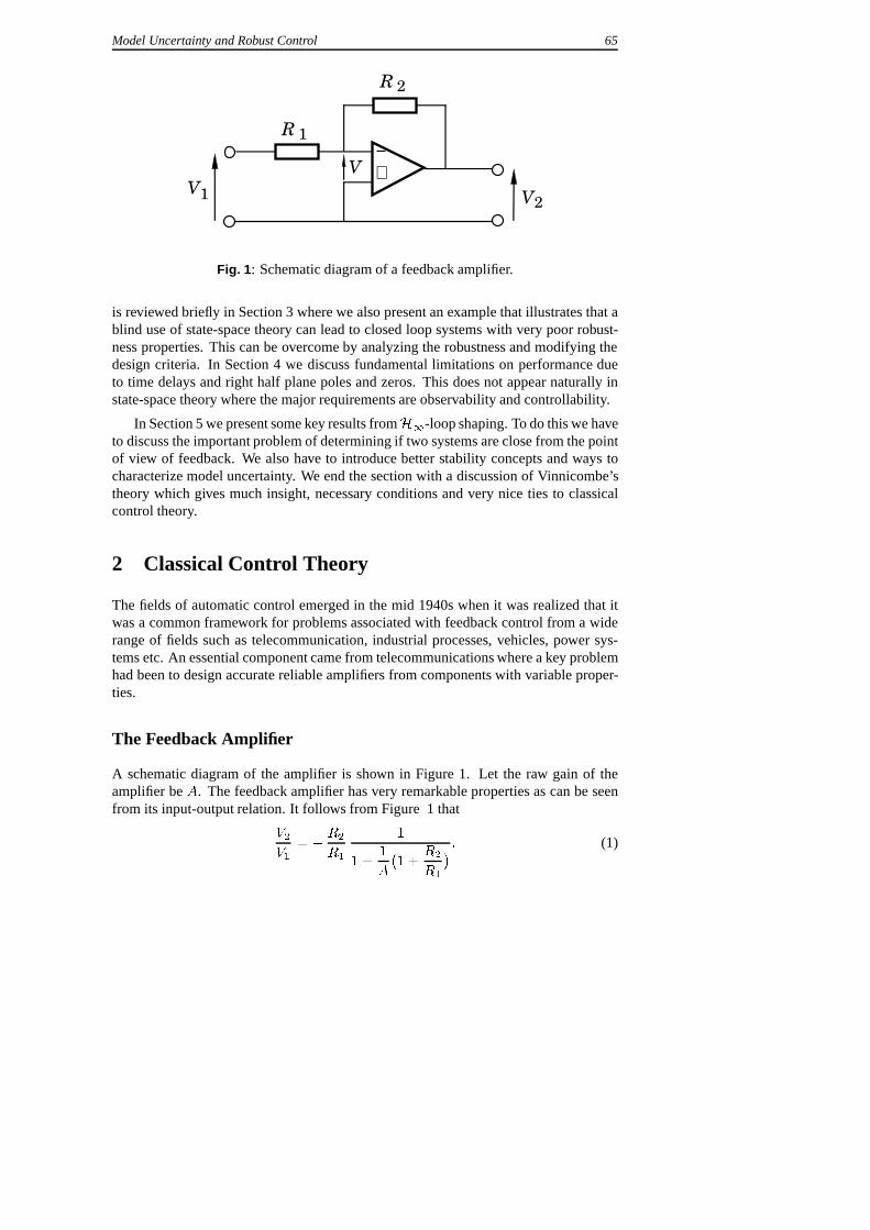
Fig. 1 : Schematic diagram of a feedback amplifier.

is reviewed briefly in Section 3 where we also present an example that illustrates that ablind use of state-space theory can lead to closed loop systems with very poor robust-ness properties. This can be overcome by analyzing the robustness and modifying thedesign criteria. In Section 4 we discuss fundamental limitations on performance dueto time delays and right half plane poles and zeros. This does not appear naturally instate-space theory where the major requirements are observability and controllability.

In Section 5 we present some key results fromH1-loop shaping. To do this we haveto discuss the important problem of determining if two systems are close from the pointof view of feedback. We also have to introduce better stability concepts and ways tocharacterize model uncertainty. We end the section with a discussion of Vinnicombe’stheory which gives much insight, necessary conditions and very nice ties to classicalcontrol theory.

2 Classical Control Theory

The fields of automatic control emerged in the mid 1940s when it was realized that itwas a common framework for problems associated with feedback control from a widerange of fields such as telecommunication, industrial processes, vehicles, power sys-tems etc. An essential component came from telecommunications where a key problemhad been to design accurate reliable amplifiers from components with variable proper-ties.

The Feedback Amplifier

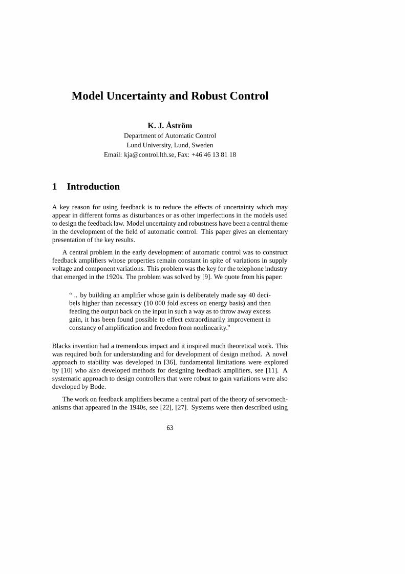
A schematic diagram of the amplifier is shown in Figure 1. Let the raw gain of theamplifier beA. The feedback amplifier has very remarkable properties as can be seenfrom its input-output relation. It follows from Figure 1 that

V2

V1= � R2

R1

1

1 +1

A

�1 +

R2

R1

� : (1)


e

-

� �� PC

`

v

n

yu xr

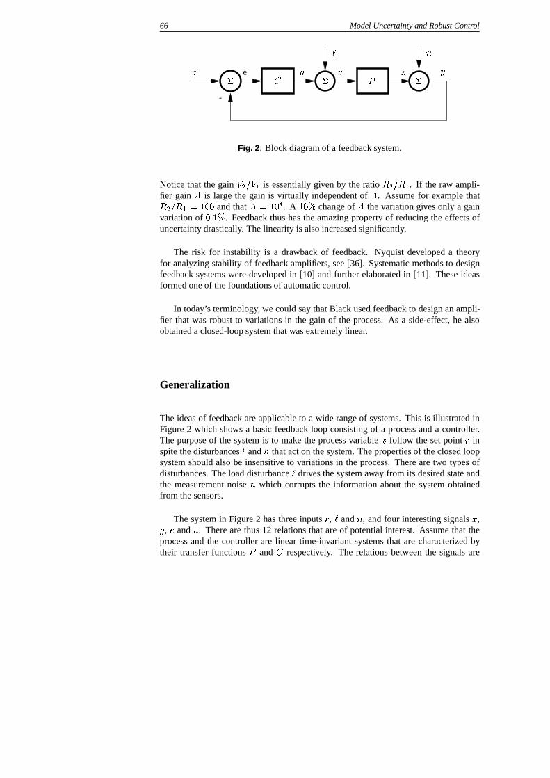
Fig. 2 : Block diagram of a feedback system.

Notice that the gainV2=V1 is essentially given by the ratioR2=R1. If the raw ampli-fier gainA is large the gain is virtually independent ofA. Assume for example thatR2=R1 = 100 and thatA = 104. A 10% change ofA the variation gives only a gainvariation of0:1%. Feedback thus has the amazing property of reducing the effects ofuncertainty drastically. The linearity is also increased significantly.

The risk for instability is a drawback of feedback. Nyquist developed a theoryfor analyzing stability of feedback amplifiers, see [36]. Systematic methods to designfeedback systems were developed in [10] and further elaborated in [11]. These ideasformed one of the foundations of automatic control.

In today’s terminology, we could say that Black used feedback to design an ampli-fier that was robust to variations in the gain of the process. As a side-effect, he alsoobtained a closed-loop system that was extremely linear.

Generalization

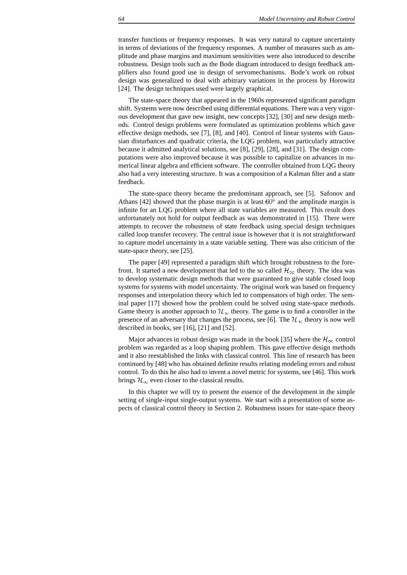
The ideas of feedback are applicable to a wide range of systems. This is illustrated inFigure 2 which shows a basic feedback loop consisting of a process and a controller.The purpose of the system is to make the process variablex follow the set pointr inspite the disturbancesandn that act on the system. The properties of the closed loopsystem should also be insensitive to variations in the process. There are two types ofdisturbances. The load disturbance` drives the system away from its desired state andthe measurement noisen which corrupts the information about the system obtainedfrom the sensors.

The system in Figure 2 has three inputsr, ` andn, and four interesting signalsx,y, e andu. There are thus 12 relations that are of potential interest. Assume that theprocess and the controller are linear time-invariant systems that are characterized bytheir transfer functionsP andC respectively. The relations between the signals are


given by the transfer functions:

Gxr =PC

1 + PCGx` =

P

1 + PCGxn = �Gxr

Gyr = Gxr Gy` = Gx` Gyn =1

1 + PC

Ger = 1�Gxr = Gyn Ge` = �Gx` Gen = �Gyn

Gur =C

1 + PCGu` = �Gxr Gun = �Gur

HereGij denotes the transfer function from signalj to signali. Notice that there areonly four independent transfer functions.

Gxr =PC

1 + PC

Gx` =P

1 + PC

Gyn =1

1 + PC

Gur =C

1 + PC

(2)

The transfer functionsGxr = T andGyn = S have special names,S is called thesensitivity function, andT is called the complementary sensitivity function. Noticethat bothS andT depend only on the loop transfer functionL = PC. The sensitivityfunctions are are related by

S + T = 1: (3)

This explains the name complementary sensitivity function. These functions have in-teresting properties as is discussed in the following.

Stability and Stability Margins

Many properties of the system in Figure 2 can be derived from the loop transfer functionL = PC.

The stability of the system can be investigated by Nyquist’s stability criterion whichsays that the closed loop system is stable if

1

2��arg

�(1 + L(s)) = �Prhp(L) (4)

where�arg is the argument variation whens traverses a contour� that encloses theright half plane (RHP) andPrhp(L) is the number of poles ofL in the right half plane.

Stability is normally investigated by analyzing the Nyquist curve, see Figure 3.


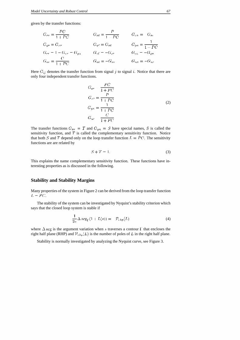
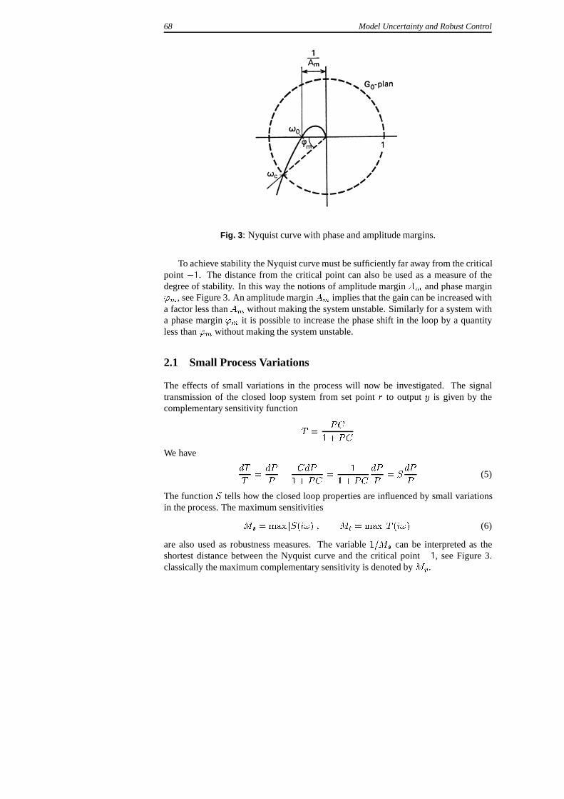
Fig. 3 : Nyquist curve with phase and amplitude margins.

To achieve stability the Nyquist curve must be sufficiently far away from the criticalpoint�1. The distance from the critical point can also be used as a measure of thedegree of stability. In this way the notions of amplitude marginAm and phase margin'm, see Figure 3. An amplitude marginAm implies that the gain can be increased witha factor less thanAm without making the system unstable. Similarly for a system witha phase margin'm it is possible to increase the phase shift in the loop by a quantityless than'm without making the system unstable.

2.1 Small Process Variations

The effects of small variations in the process will now be investigated. The signaltransmission of the closed loop system from set pointr to outputy is given by thecomplementary sensitivity function

T =PC

1 + PC

We have

dT

T=dP

P� CdP

1 + PC=

1

1 + PC

dP

P= S

dP

P(5)

The functionS tells how the closed loop properties are influenced by small variationsin the process. The maximum sensitivities

Ms = max jS(i!)j; Mt = max jT (i!)j (6)

are also used as robustness measures. The variable1=Ms can be interpreted as theshortest distance between the Nyquist curve and the critical point�1, see Figure 3.classically the maximum complementary sensitivity is denoted byMp.


−2 −1.5 −1 −0.5 0 0.5 1−2

−1.5

−1

−0.5

0

0.5

1

Im

Re

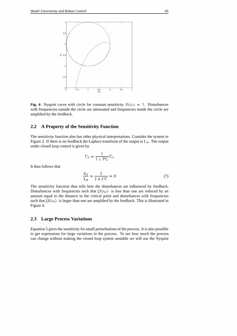
Fig. 4 : Nyquist curve with circle for constant sensitivityS(i!) = 1. Disturbanceswith frequencies outside the circle are attenuated and frequencies inside the circle areamplified by the feedback.

2.2 A Property of the Sensitivity Function

The sensitivity function also has other physical interpretations. Consider the system inFigure 2. If there is no feedback the Laplace transform of the output isYol. The outputunder closed loop control is given by

Ycl =1

1 + PCYol

It thus follows that

Ycl

Yol=

1

1 + PC= S (7)

The sensitivity function thus tells how the disturbances are influenced by feedback.Disturbances with frequencies such thatjS(i!)j is less than one are reduced by anamount equal to the distance to the critical point and disturbances with frequenciessuch thatjS(i!)j is larger than one are amplified by the feedback. This is illustrated inFigure 4.

2.3 Large Process Variations

Equation 5 gives the sensitivity for small perturbations of the process. It is also possibleto get expressions for large variations in the process. To see how much the processcan change without making the closed loop system unstable we will use the Nyquist


diagram. Consider a point on the Nyquist curve in Figure 4. The distance to the criticalpoint isj1+Lj. If the process changes by�P , the point changes byC�P . The systemwill remain stable as long as

jC�P j < j1 + PCj

and the number of right hand poles ofPC does not change. This implies that theperturbations must have the property that�P does not have any poles in the right halfplane.

The admissible variation is process dynamics is thus given by

j�PPj <

��1 + PC

PC

�� = �� 1T

�� 1

Mt(8)

which can also be expressed as

j�P j <��PT

�� jP jMt

(9)

A crude estimate of the largest admissible variation in the process is thus given by thelargest valueMt of the complementary sensitivity. It follows from the Figure 4 thatlarge variations inP are permitted for the frequencies whereP either is large or small.The smallest admissible variations are for frequencies wherejT j is large.

A similar estimate based on the maximum sensitivity is that

j�P j <�� 1

SC

�� 1

MsjCj(10)

Bode’s Integrals

It follows from Equations (5) and (8) that it would be highly desirable to make thesensitivity functionsS andT as small as possible. This is unfortunately not possiblebecause it follows from Equation (3) thatS + T = 1. There are also other constraintson the sensitivities. It was shown in [11] thatZ

1

0

log jS(i!)jd! =

Z1

0

log j 1

1 + L(i!)jd! = �

XpiZ

1

0

log jT (1=i!)jd! =

Z1

0

log j L(1=i!)

1 + L(1=i!)jd! = �

X 1

zi

(11)

wherepi are the right half plane poles ofL andzi are the right half plane zeros ofL. These equations imply that the sensitivities can be made small at one frequencyonly at the expense of increasing the sensitivity at other frequencies. This phenomenais sometimes called the water bed effect. It also follows from the equations that thepresence of poles in the right half plane increase the sensitivity and that zeros in theright half plane increase the complementary sensitivity. A fast RHP pole gives highersensitivity than a slow pole, and a slow RHP zero gives higher sensitivity than a fastzero.


2.4 Bode’s Relations

The amplitude and the phase curves are also related. It is not possible to achieve highphase advance without using high gains and it is not possible to obtain transfer func-tions that decrease rapidly without having large phase lags. These facts are expressedanalytically by some relations derived in [10].

Consider a transfer functionG(s) with no poles or zeros in the right half plane.Introduce

logG(i!) = A(!) + i�(!) (12)

a logarithmic frequency scaleu = log!=!0, ! = !0eu, and the functions

a(u) = A(!0eu); �(u) = �(!0e

u):

Assume that(logG(s))=s goes to zero ass goes to infinity, then

A(!0)�A(1) = � 2

�

Z1

0

v�(v)� !0�(!0)

v2 � !2

0

dv

= � 1

!0�

Z1

�1

d(eu�(u))

dulog coth ju

2jdu

�(!0) =2!0

�

Z1

0

A(v) �A(!0)

v2 � !2

0

dv =1

�

Z1

�1

da(u)

dulog coth ju

2jdu

(13)

an approximate version is that

�(!) � 2

�

da(u)

du: (14)

This means that if the slopen = da(u)=du of the magnitude curve is constant the phaseis n�=2. This relation appears in practically all elementary courses in feedback control.

Bode’s relations imposes fundamental limitations on the performance that can beachieved. A simple observation is that even if it is desirable that the loop gain decreasesrapidly at the crossover frequency, it is not possible to have a steeper slope than -2without violating stability constraints.

An interesting problem is if the limitations imposed by Bode’s relations can beavoided by using nonlinear systems. The Clegg integrator [13] is a nonlinear systemwhere the magnitude curve has the slope -1 and the phase lag is only38Æ.

2.5 Bode’s Ideal Loop Transfer Function

In his work on design of feedback amplifiers Bode suggested an ideal shape of the looptransfer function. He proposed that the loop transfer function should have the form

L(s) =� s

!gc

�n: (15)


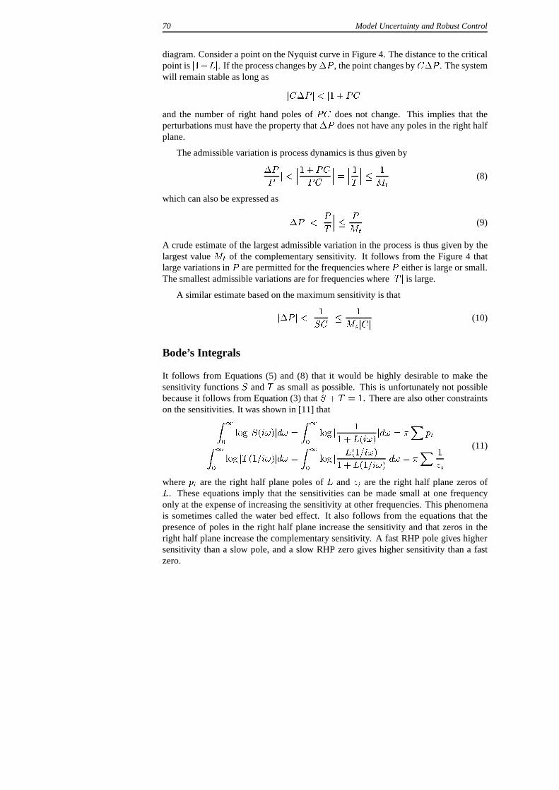
Fig. 5 : Nyquist curve for Bode’s ideal loop transfer function.

The Nyquist curve for this loop transfer function is simply a straight line through theorigin with argL(i!) = n�=2, see Figure 5. Bode called (15) the ideal cut-off char-acteristic. In the terminology of automatic control we will call it Bode’s ideal looptransfer function.

One reason why Bode made the particular choice ofL(s) given by Equation (15)is that it gives a closed-loop system that is insensitive to gain changes. Changes inthe process gain will change the crossover frequency but the phase margin is'm =

�(1 + n=2) for all values of the gain. The amplitude margin is infinite. The slopesn =

�1:333, �1:5 and�1:667 correspond to phase margins of60Æ, 45Æ and30Æ. Bode’sidea to use loop shaping to design controller that are insensitive to gain variations werelater generalized by [24] to systems that are insensitive to other variations of the plant,culminating in the QFT method, see [26].

The transfer function given by Equation (15) is an irrational transfer function fornon-integern. It can be approximated arbitrarily close by rational frequency functions.Bode also suggested that it was sufficient to approximateL over a frequency rangearound the desired crossover frequency!gc. Assume for example that the gain of theprocess varies betweenkmin andkmax and that it is desired to have a loop transferfunction that is close to (15) in the frequency range(!min; !max). It follows from (15)that

!max

!min=�kmax

kmin

�1=n

With n = �5=3 and a gain ratio of 100 we get a frequency ratio of about 16 and withn = �4=3we get a frequency ratio of 32. To avoid having too large a frequency range itis thus useful to haven as small as possible. There is, however, a compromise becausethe phase margin decreases with decreasingn and the system becomes unstable forn = �2.


2.6 Fractional Systems

It follows from Equation (15) that the loop transfer function is not a rational function.We illustrate this with an example.

Example.

Consider a process with the transfer function

P (s) =k

s(s+ 1)(16)

Assume that we would like to have a closed loop system that is insensitive to gainvariations with a phase margin of45Æ. Bode’s ideal loop transfer function that givesthis phase margin is

L(s) =1

sps

(17)

SinceL = PC we find that the controller transfer function is

C(s) =s+ 1p

s=ps+

1ps

(18)

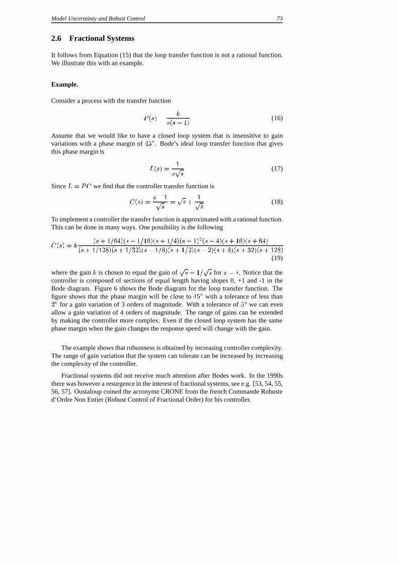
To implement a controller the transfer function is approximated with a rational function.This can be done in many ways. One possibility is the following

C(s) = k(s+ 1=64)(s+ 1=16)(s+ 1=4)(s+ 1)2(s+ 4)(s+ 16)(s+ 64)

(s+ 1=128)(s+ 1=32)(s+ 1=8)(s+ 1=2)(s+ 2)(s+ 8)(s+ 32)(s+ 128)

(19)

where the gaink is chosen to equal the gain ofps + 1=

ps for s = i. Notice that the

controller is composed of sections of equal length having slopes 0, +1 and -1 in theBode diagram. Figure 6 shows the Bode diagram for the loop transfer function. Thefigure shows that the phase margin will be close to45Æ with a tolerance of less than2Æ for a gain variation of 3 orders of magnitude. With a tolerance of5Æ we can evenallow a gain variation of 4 orders of magnitude. The range of gains can be extendedby making the controller more complex. Even if the closed loop system has the samephase margin when the gain changes the response speed will change with the gain.

The example shows that robustness is obtained by increasing controller complexity.The range of gain variation that the system can tolerate can be increased by increasingthe complexity of the controller.

Fractional systems did not receive much attention after Bodes work. In the 1990sthere was however a resurgence in the interest of fractional systems, see e.g. [53, 54, 55,56, 57]. Oustaloup coined the acronyme CRONE from the french Commande Robusted’Ordre Non Entier (Robust Control of Fractional Order) for his controller.


-100

-50

0

50

100

10-2 10-1 100 101 102-150

-140

-130

-120

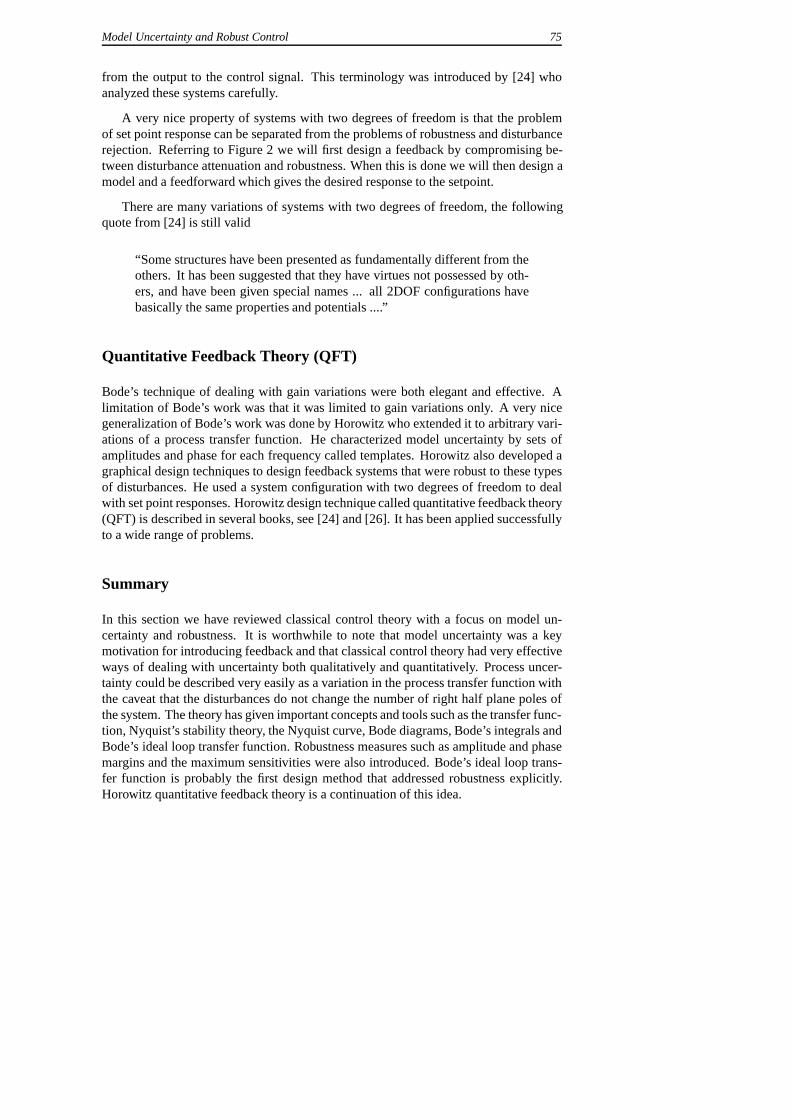
Fig. 6 : Bode diagram of the loop transfer function obtained by approximating the frac-tional controller with a rational transfer function.

y c uΣModele y

−1

Process y sp

Feedforward

ΣController

uff

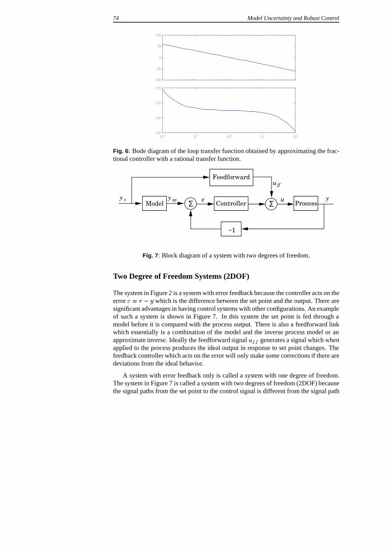
Fig. 7 : Block diagram of a system with two degrees of freedom.

Two Degree of Freedom Systems (2DOF)

The system in Figure 2 is a system with error feedback because the controller acts on theerrore = r � y which is the difference between the set point and the output. There aresignificant advantages in having control systems with other configurations. An exampleof such a system is shown in Figure 7. In this system the set point is fed through amodel before it is compared with the process output. There is also a feedforward linkwhich essentially is a combination of the model and the inverse process model or anapproximate inverse. Ideally the feedforward signaluff generates a signal which whenapplied to the process produces the ideal output in response to set point changes. Thefeedback controller which acts on the error will only make some corrections if there aredeviations from the ideal behavior.

A system with error feedback only is called a system with one degree of freedom.The system in Figure 7 is called a system with two degrees of freedom (2DOF) becausethe signal paths from the set point to the control signal is different from the signal path


from the output to the control signal. This terminology was introduced by [24] whoanalyzed these systems carefully.

A very nice property of systems with two degrees of freedom is that the problemof set point response can be separated from the problems of robustness and disturbancerejection. Referring to Figure 2 we will first design a feedback by compromising be-tween disturbance attenuation and robustness. When this is done we will then design amodel and a feedforward which gives the desired response to the setpoint.

There are many variations of systems with two degrees of freedom, the followingquote from [24] is still valid

“Some structures have been presented as fundamentally different from theothers. It has been suggested that they have virtues not possessed by oth-ers, and have been given special names ... all 2DOF configurations havebasically the same properties and potentials ....”

Quantitative Feedback Theory (QFT)

Bode’s technique of dealing with gain variations were both elegant and effective. Alimitation of Bode’s work was that it was limited to gain variations only. A very nicegeneralization of Bode’s work was done by Horowitz who extended it to arbitrary vari-ations of a process transfer function. He characterized model uncertainty by sets ofamplitudes and phase for each frequency called templates. Horowitz also developed agraphical design techniques to design feedback systems that were robust to these typesof disturbances. He used a system configuration with two degrees of freedom to dealwith set point responses. Horowitz design technique called quantitative feedback theory(QFT) is described in several books, see [24] and [26]. It has been applied successfullyto a wide range of problems.

Summary

In this section we have reviewed classical control theory with a focus on model un-certainty and robustness. It is worthwhile to note that model uncertainty was a keymotivation for introducing feedback and that classical control theory had very effectiveways of dealing with uncertainty both qualitatively and quantitatively. Process uncer-tainty could be described very easily as a variation in the process transfer function withthe caveat that the disturbances do not change the number of right half plane poles ofthe system. The theory has given important concepts and tools such as the transfer func-tion, Nyquist’s stability theory, the Nyquist curve, Bode diagrams, Bode’s integrals andBode’s ideal loop transfer function. Robustness measures such as amplitude and phasemargins and the maximum sensitivities were also introduced. Bode’s ideal loop trans-fer function is probably the first design method that addressed robustness explicitly.Horowitz quantitative feedback theory is a continuation of this idea.


3 State-Space Theory

The state-space theory represented a paradigm shift which led to many useful systemconcepts and new methods for analysis and design. The systems was represented bydifferential equations instead of transfer functions. For linear systems the standardmodel used was

dx

dt= Ax +Bu+ v

y = Cx + e

(20)

whereu is the input,y the output andx is the state. The uncertainty is represented bythe disturbancesv ande and by variations in the elements of the matricesA, B andC.The disturbancese andv were typically described as stochastic processes, see [20] and[4].

The control problem was formulated as to minimize the criterion

J = E limT!1

1

T

Z T

0

(xTQ1x+ uTQ2u)dt (21)

Since the equations are linear with stochastic disturbances and the criterion is quadraticthe problem was called the linear quadratic Gaussian control problem (LQG). The so-lution to the control problem is given by

u = L(xm � x) + uff

dx

dt= Ax+Bu+K(y � Cx)

(22)

This control law has a very nice interpretation as feedback from the errorxm � x

which is the difference between the ideal statesxm and the estimated statesx. Theestimated states are given by the Kalman filter. Controllability and observability arekey conditions for solving the problem.

There are many other design methods based on the state-space formulation whichgives controllers with the structure (22) for example pole placement. They differ fromthe LQG method in the sense that other techniques are used to obtain the matricesK

andL.

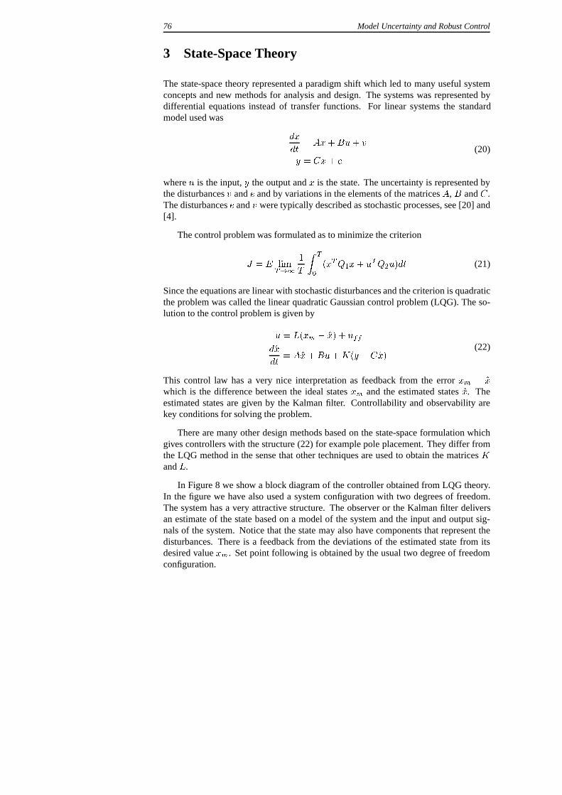
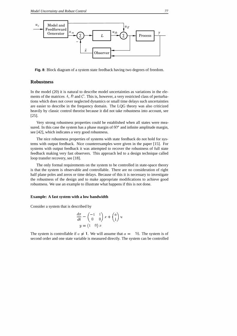
In Figure 8 we show a block diagram of the controller obtained from LQG theory.In the figure we have also used a system configuration with two degrees of freedom.The system has a very attractive structure. The observer or the Kalman filter deliversan estimate of the state based on a model of the system and the input and output sig-nals of the system. Notice that the state may also have components that represent thedisturbances. There is a feedback from the deviations of the estimated state from itsdesired valuexm. Set point following is obtained by the usual two degree of freedomconfiguration.


∑ ∑x m

uff

ˆ x Observer

L Process

−

ufb y

uc Model andFeedforward Generator

Fig. 8 : Block diagram of a system state feedback having two degrees of freedom.

Robustness

In the model (20) it is natural to describe model uncertainties as variations in the ele-ments of the matricesA,B andC. This is, however, a very restricted class of perturba-tions which does not cover neglected dynamics or small time delays such uncertaintiesare easier to describe in the frequency domain. The LQG theory was also criticizedheavily by classic control theorist because it did not take robustness into account, see[25].

Very strong robustness properties could be established when all states were mea-sured. In this case the system has a phase margin of60Æ and infinite amplitude margin,see [42], which indicates a very good robustness.

The nice robustness properties of systems with state feedback do not hold for sys-tems with output feedback. Nice counterexamples were given in the paper [15]. Forsystems with output feedback it was attempted to recover the robustness of full statefeedback making very fast observers. This approach led to a design technique calledloop transfer recovery, see [18].

The only formal requirements on the system to be controlled in state-space theoryis that the system is observable and controllable. There are no consideration of righthalf plane poles and zeros or time delays. Because of this it is necessary to investigatethe robustness of the design and to make appropriate modifications to achieve goodrobustness. We use an example to illustrate what happens if this is not done.

Example: A fast system with a low bandwidth

Consider a system that is described by

dx

dt=

��1 1

0 0

�x+

�a

1

�u

y =�1 0

�x

The system is controllable ifa 6= 1. We will assume thata = �10. The system is ofsecond order and one state variable is measured directly. The system can be controlled


with an observer of first degree. The closed loop system is then of order 3. We assumethat a state feedback and an observe is designed so that the closed loop system is

(s+ �!0)(s2 + !0s+ !2

0): (23)

The transfer function of the system is

P (s) =as+ 1

s(s+ 1): (24)

To obtain a fast closed-loop system we choose!0 = 10 and� = 1. straightforwardcalculations show that the controller has the transfer function

C(s) =s0s+ s1

s+ r(25)

with r = 9274:5, s0 = 925:5 ands1 = 1000. The loop transfer function is

L(s) =(as+ 1)(s0s+ s1)

s(s+ 1)(s+ r)= �9255(s� 0:1)(s+ 1:0805)

s(s+ 1)(s+ 9274):

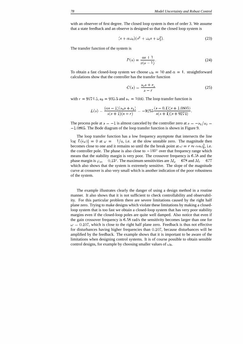
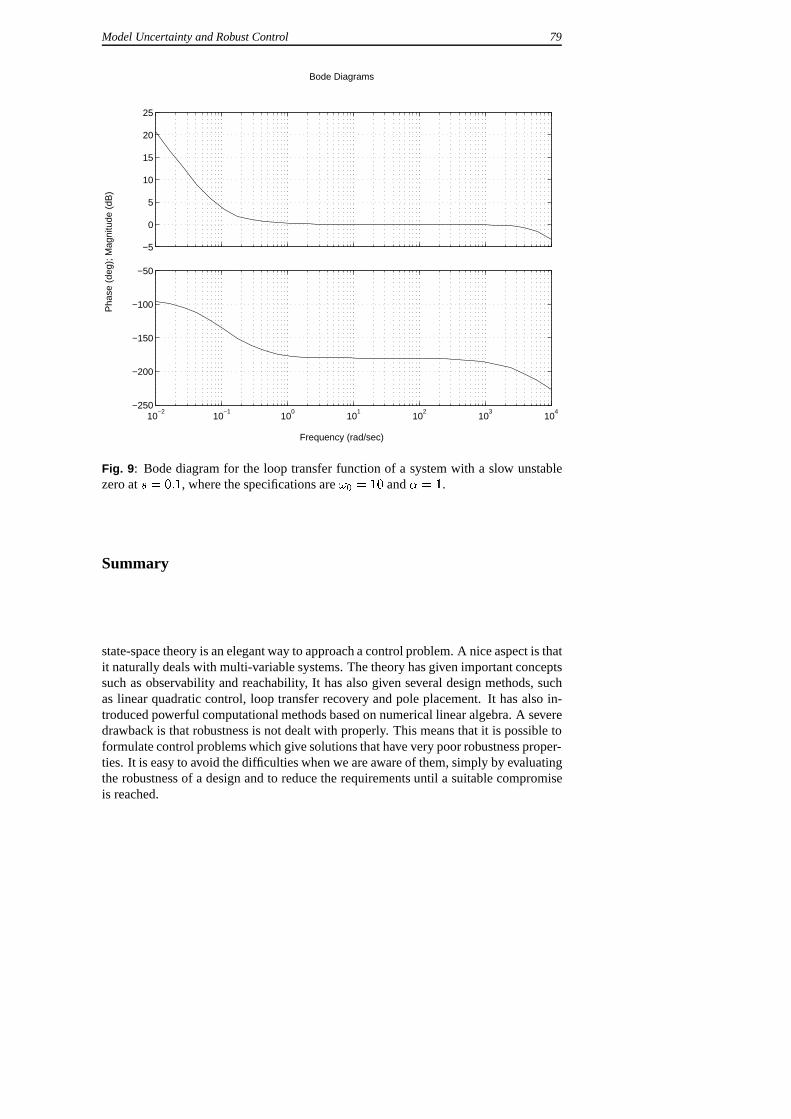
The process pole ats = �1 is almost canceled by the controller zero ats = �s1=s0 =�1:0805. The Bode diagram of the loop transfer function is shown in Figure 9.

The loop transfer function has a low frequency asymptote that intersects the linelog jL(i!)j = 0 at ! = �1=a, i.e. at the slow unstable zero. The magnitude thenbecomes close to one and it remains so until the the break point at! = r � �a!3

0, i.e.

the controller pole. The phase is also close to�180Æ over that frequency range whichmeans that the stability margin is very poor. The crossover frequency is6:58 and thephase margin is'm = 0:15Æ. The maximum sensitivities areMs = 678 andMt = 677

which also shows that the system is extremely sensitive. The slope of the magnitudecurve at crossover is also very small which is another indication of the poor robustnessof the system.

The example illustrates clearly the danger of using a design method in a routinemanner. It also shows that it is not sufficient to check controllability and observabil-ity. For this particular problem there are severe limitations caused by the right halfplane zero. Trying to make designs which violate these limitations by making a closed-loop system that is too fast we obtain a closed-loop system that has very poor stabilitymargins even if the closed-loop poles are quite well damped. Also notice that even ifthe gain crossover frequency is6:58 rad/s the sensitivity becomes larger than one for! = 0:107, which is close to the right half plane zero. Feedback is thus not effectivefor disturbances having higher frequencies than0:107, because disturbances will beamplified by the feedback. The example shows that it is important to be aware of thelimitations when designing control systems. It is of course possible to obtain sensiblecontrol designs, for example by choosing smaller values of!0.


Frequency (rad/sec)

Pha

se (

deg)

; Mag

nitu

de (

dB)

Bode Diagrams

−5

0

5

10

15

20

25

10−2

10−1

100

101

102

103

104

−250

−200

−150

−100

−50

Fig. 9 : Bode diagram for the loop transfer function of a system with a slow unstablezero ats = 0:1, where the specifications are!0 = 10 and� = 1.

Summary

state-space theory is an elegant way to approach a control problem. A nice aspect is thatit naturally deals with multi-variable systems. The theory has given important conceptssuch as observability and reachability, It has also given several design methods, suchas linear quadratic control, loop transfer recovery and pole placement. It has also in-troduced powerful computational methods based on numerical linear algebra. A severedrawback is that robustness is not dealt with properly. This means that it is possible toformulate control problems which give solutions that have very poor robustness proper-ties. It is easy to avoid the difficulties when we are aware of them, simply by evaluatingthe robustness of a design and to reduce the requirements until a suitable compromiseis reached.


4 Fundamental Limitations

It is very useful to determine the performance that can be achieved without sacrificingrobustness. Such estimates will be provided in this section. In particular we will con-sider limitations that arise from poles and zeros in the right half plane and time delays.The results are based on [2] and [1].

Consider a system with the transfer functionP (s). Factor the transfer function as

P (s) = Pmp(s)Pnmp(s) (26)

wherePmp is the minimum phase part andPnmp is the non-minimum phase part. Let�P (s) denote the uncertainty in the process transfer function. It is assumed that thefactorization is normalized so thatjPnmp(i!)j = 1 and the sign is chosen so thatPnmp

has negative phase. The achievable bandwidth is characterized by the gain crossoverfrequency!gc.

4.1 The Crossover Frequency Inequality

We will now derive an inequality for the gain crossover frequency. The loop transferfunction isL(s) = P (s)C(s). Requiring that the phase margin is'm we get.

argL(i!gc) = argPnmp(i!gc) + argPmp(i!gc) + argC(i!gc) � �� + 'm: (27)

Assume that the controller is chosen so that the loop transfer functionPmpC is equal toBode’s ideal loop transfer function given by Equation (15), then

argPmp(i!) + argC(i!) = n�

2(28)

wheren is the slope of the loop transfer function at the crossover frequency. Equa-tion (28) is also a good approximation for other controllers because the amplitude curveis typically close to a straight line at the crossover frequency. The parametern in (28)is then the slopengc at the crossover frequency. It follows from Bode’s relations (13)that the phase isngc�=2. It follows from Equations (27) and (28) that the crossoverfrequency satisfies the inequality

argPnmp(i!gc) � ��; (29)

where

� = � � 'm + ngc�

2: (30)

Thiscrossover frequency inequalitygives the limitations imposed by non-minimumphase factors. A straightforward method to determine the crossover frequencies thatcan be obtained is to plot the left hand side of Equation (29) and determine when theinequality holds. The following example gives a simple rule of thumb.


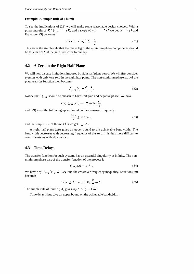
Example: A Simple Rule of Thumb

To see the implications of (29) we will make some reasonable design choices. With aphase margin of45Æ ('m = �=4), and a slope ofngc = �1=2 we get� = �=2 andEquation (29) becomes

argPnmp(i!gc) � ��

2: (31)

This gives the simple rule that the phase lag of the minimum phase components shouldbe less than90Æ at the gain crossover frequency.

4.2 A Zero in the Right Half Plane

We will now discuss limitations imposed by right half plane zeros. We will first considersystems with only one zero in the right half plane. The non-minimum phase part of theplant transfer function then becomes

Pnmp(s) =z � s

z + s: (32)

Notice thatPnmp should be chosen to have unit gain and negative phase. We have

argPnmp(i!) = �2 arctan !z:

and (29) gives the following upper bound on the crossover frequency.

!gc

z� tan�=2: (33)

and the simple rule of thumb (31) we get!gc < z.

A right half plane zero gives an upper bound to the achievable bandwidth. Thebandwidth decreases with decreasing frequency of the zero. It is thus more difficult tocontrol systems with slow zeros.

4.3 Time Delays

The transfer function for such systems has an essential singularity at infinity. The non-minimum phase part of the transfer function of the process is

Pnmp(s) = e�sT : (34)

We haveargPnmp(i!) = �!T and the crossover frequency inequality, Equation (29)becomes

!gcT � � � 'm + ngc�

2= �: (35)

The simple rule of thumb (31) gives!gcT � �2= 1:57.

Time delays thus give an upper bound on the achievable bandwidth.


4.4 A Pole in the Right Half Plane

Consider a system with one pole in the right half plane. The non-minimum phase partof the transfer function is thus

Pnmp(s) =s+ p

s� p(36)

wherep > 0. Notice that the transfer function is normalized so thatPnmp has unit gainand negative phase. We have

argPnmp(i!) = �2 arctan p

!:

and the crossover frequency inequality] (29) gives

!gc �p

tan�=2: (37)

The simple rule of thumb (31) gives!gc � p.

Unstable poles give a lower bound on the crossover frequency. For systems withright half plane poles the bandwidth must thus be sufficiently large.

4.5 Poles and Zeros in the Right Half Plane

Consider a system with

Pnmp(s) =(z � s)(s+ p)

(z + s)(s� p): (38)

Forz > p we have

argPnmp(i!) = �2 arctan !z� 2 arctan

p

!= �2 arctan !=z + p=!

1� p=z:

The right hand side has its maximum for! =ppz and the inequality (29) becomes

z

p� tan2 �=2 = tan2

��4� 'm

4+ ngc

�

8

�: (39)

The simple rule of thumb (31) givesz � 25:3p. Table 1 gives the phase margin as afunction of the ratioz=p for 'm = �=4 andngc = �1=2. The phase-margin that canbe achieved for a given ratiop=z is

'm < � + ngc�

2� 4 arctan

rp

z: (40)

When the unstable zero is faster than the unstable pole, i.e.z > p, the ratioz=pthus must be sufficiently large in order to have the desired phase margin. The largestgain crossover frequency is the geometric mean of the unstable pole and zero.


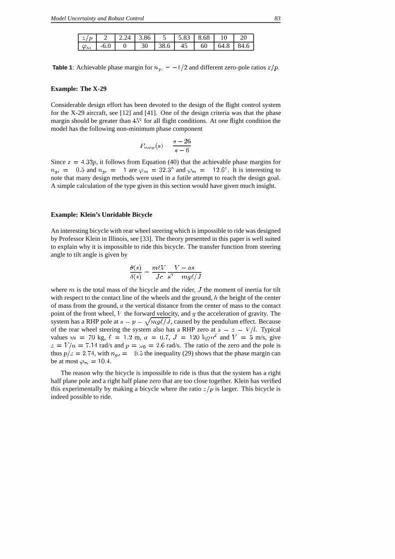
z=p 2 2.24 3.86 5 5.83 8.68 10 20'm -6.0 0 30 38.6 45 60 64.8 84.6

Table 1 : Achievable phase margin forngc = �1=2 and different zero-pole ratiosz=p.

Example: The X-29

Considerable design effort has been devoted to the design of the flight control systemfor the X-29 aircraft, see [12] and [41]. One of the design criteria was that the phasemargin should be greater than45Æ for all flight conditions. At one flight condition themodel has the following non-minimum phase component

Pnmp(s) =s� 26

s� 6

Sincez = 4:33p, it follows from Equation (40) that the achievable phase margins forngc = �0:5 andngc = �1 are'm = 32:3Æ and'm = �12:6Æ. It is interesting tonote that many design methods were used in a futile attempt to reach the design goal.A simple calculation of the type given in this section would have given much insight.

Example: Klein’s Unridable Bicycle

An interesting bicycle with rear wheel steering which is impossible to ride was designedby Professor Klein in Illinois, see [33]. The theory presented in this paper is well suitedto explain why it is impossible to ride this bicycle. The transfer function from steeringangle to tilt angle is given by

�(s)

Æ(s)=m`V

Jc

V � as

s2 �mg`=J

wherem is the total mass of the bicycle and the rider,J the moment of inertia for tiltwith respect to the contact line of the wheels and the ground,h the height of the centerof mass from the ground,a the vertical distance from the center of mass to the contactpoint of the front wheel,V the forward velocity, andg the acceleration of gravity. Thesystem has a RHP pole ats = p =

pmg`=J , caused by the pendulum effect. Because

of the rear wheel steering the system also has a RHP zero ats = z = V=l. Typicalvaluesm = 70 kg, ` = 1:2 m, a = 0:7, J = 120 kgm2 andV = 5 m/s, givez = V=a = 7:14 rad/s andp = !0 = 2:6 rad/s. The ratio of the zero and the pole isthusp=z = 2:74, with ngc = �0:5 the inequality (29) shows that the phase margin canbe at most'm = 10:4.

The reason why the bicycle is impossible to ride is thus that the system has a righthalf plane pole and a right half plane zero that are too close together. Klein has verifiedthis experimentally by making a bicycle where the ratioz=p is larger. This bicycle isindeed possible to ride.


So far we have only discussed the casez > p. When the unstable zero is slowerthan the unstable pole the crossover frequency inequality (29) cannot be satisfied unless'm < 0 andngc > 0.

4.6 A Pole in the Right Half Plane and Time Delay

Consider a system with one pole in the right half plane and a time delayT . The non-minimum phase part of the transfer function is thus

Pnmp(s) =s+ p

s� pe�sT : (41)

The crossover frequency condition (29) gives

2 arctan!gc

p� !gcT � 'm � ngc

�

2: (42)

The system cannot be stabilized ifpT > 2. If pT < 2 the left hand side has its smallestvalue for!gc=p =

p2=(pT )� 1. Introducing this value of!gc into (42) we get

2 arctan

r2

pT� 1� pT

r2

pT� 1 > 'm � ngc

�

2:

The simple rule of thumb with to'm = �=4 andngc = �0:5 gives

pT � 0:326 (43)

Example: Pole balancing

To illustrate the results we can consider balancing of an inverted pendulum. A pendu-lum of length` has a right half plane pole

pg=`. Assuming that the neural lag of a

human is0:07 s. The inequality (43) givespg=` 0:07 < 0:326, hence > 0:45. The

calculation thus indicate that a human with a lag of 0.07 s should be able to balancea pendulum whose length is 0.5 m. To balance a pendulum whose length is 0.1 m thetime delay must be less than 0.03s. Pendulum balancing has also been done using videocameras as angle sensors. The limited video rate imposes strong limitations on what canbe achieved. With a video rate of 20 Hz it follows from (43) that the shortest pendulumthat can be balanced with'm = 45Æ andngc = �0:5 is ` = 0:23m.

4.7 Other Criteria

The phase margin is a crude indicator of the stability margin. By carrying out detaileddesigns the results can be refined. This is done in [1] which gives results for designswith Ms =Mt = 2 andMs =Mt = 1:4.


� A RHP zeroz

!gc

z�(0:5 for Ms,Mt < 2

0:2 for Ms,Mt < 1:4:

� A RHP polep

p

!gc�(2 for Ms, Mt < 2

5 for Ms, Mt < 1:4:

� A time delayT

!gcT �(0:7 for Ms,Mt < 2

0:37 for Ms,Mt < 1:4:

� A RHP pole-zero pair withz > p

z

p�(6:5 for Ms,Mt < 2

14:4 for Ms,Mt < 1:4:

� A RHP polep and a time delayT

pT �(0:16 for Ms, Mt < 2

0:05 for Ms, Mt < 1:4:

A time delay or a zero in the right half plane gives an upper bound of the bandwidth thatcan be achieved. The bound decreases when the zeroz decreases and the time delayincreases. A pole in the right half plane gives a lower bound on the bandwidth. Thebandwidth increases with increasingp. For a pole zero pair there is a upper bound onthe pole-zero ratio.

5 H1 Loop Shaping

A consequence of the introduction of state-space theory was that interest shifted fromrobustness to optimization. New developments that started by the development ofH1control by George Zames in the 1980s gave a strong revival of robustness, see [50]. Thisled to a very vigorous development that has given new insight and new design methods.These results will be discussed in this Section. To keep the presentation simple wewill only deal with systems having one input and one output, but techniques as well asresults can be generalized to systems with many inputs and many outputs. For moreextensive treatments we refer to [16], [21], [52] [23] and [48].


� �

P

�C

`

v

n

yu

x

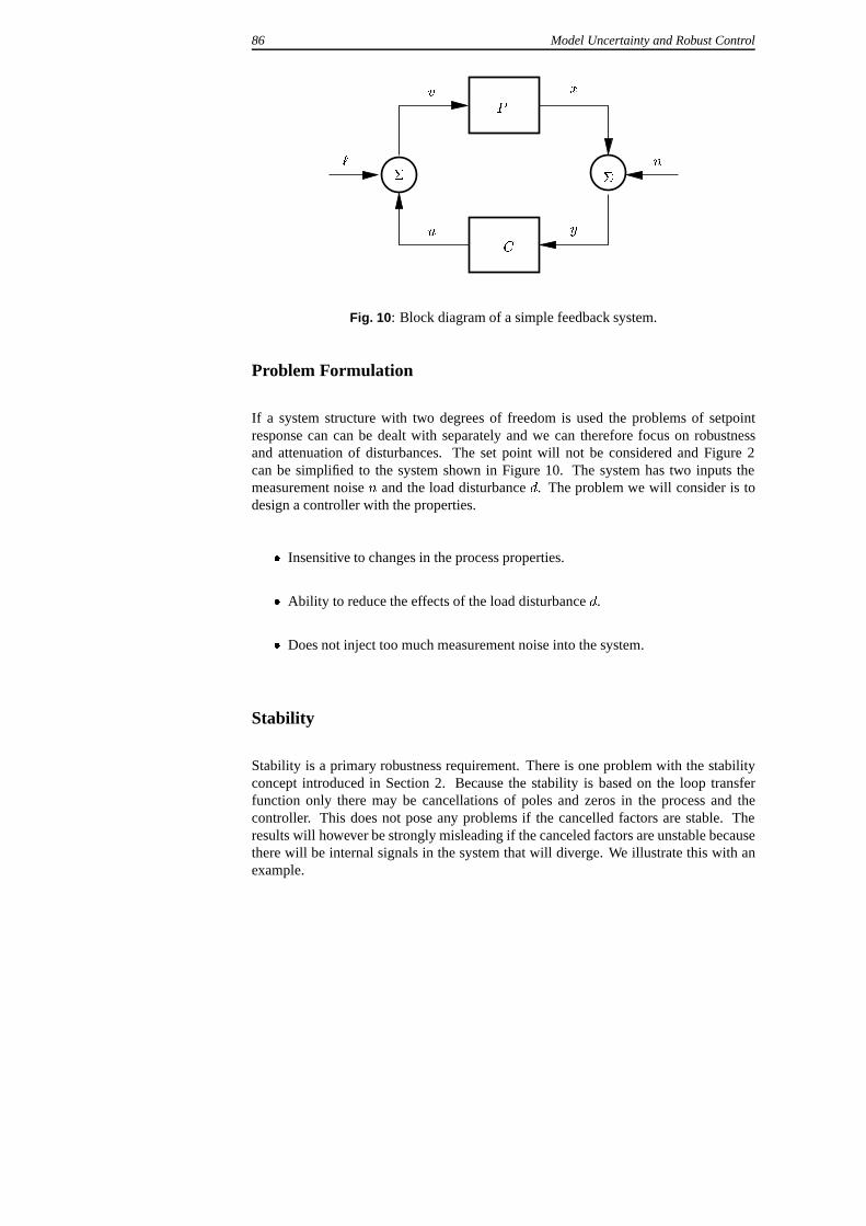
Fig. 10 : Block diagram of a simple feedback system.

Problem Formulation

If a system structure with two degrees of freedom is used the problems of setpointresponse can can be dealt with separately and we can therefore focus on robustnessand attenuation of disturbances. The set point will not be considered and Figure 2can be simplified to the system shown in Figure 10. The system has two inputs themeasurement noisen and the load disturbanced. The problem we will consider is todesign a controller with the properties.

� Insensitive to changes in the process properties.

� Ability to reduce the effects of the load disturbanced.

� Does not inject too much measurement noise into the system.

Stability

Stability is a primary robustness requirement. There is one problem with the stabilityconcept introduced in Section 2. Because the stability is based on the loop transferfunction only there may be cancellations of poles and zeros in the process and thecontroller. This does not pose any problems if the cancelled factors are stable. Theresults will however be strongly misleading if the canceled factors are unstable becausethere will be internal signals in the system that will diverge. We illustrate this with anexample.


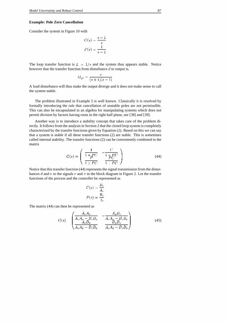
Example: Pole Zero Cancellation

Consider the system in Figure 10 with

C(s) =s� 1

s

P (s) =1

s� 1

The loop transfer function isL = 1=s and the system thus appears stable. Noticehowever that the transfer function from disturbanced to output is.

Gy` =s

(s+ 1)(s� 1)

A load disturbance will thus make the output diverge and it does not make sense to callthe system stable.

The problem illustrated in Example 5 is well known. Classically it is resolved byformally introducing the rule that cancellation of unstable poles are not permissible.This can also be encapsulated in an algebra for manipulating systems which does notpermit division by factors having roots in the right half plane, see [38] and [39].

Another way is to introduce a stability concept that takes care of the problem di-rectly. It follows from the analysis in Section 2 that the closed loop system is completelycharacterized by the transfer functions given by Equation (2). Based on this we can saythat a system is stable if all these transfer functions (2) are stable. This is sometimescalled internal stability. The transfer functions (2) can be conveniently combined in thematrix

G(s) =

0B@

1

1 + PC� C

1 + PCP

1 + PC� PC

1 + PC

1CA (44)

Notice that this transfer function (44) represents the signal transmission from the distur-bancesd andn to the signalsv andx in the block diagram in Figure 2. Let the transferfunctions of the process and the controller be represented as

C(s) =Bc

Ac

P (s) =Bc

Ac

The matrix (44) can then be represented as

G(s) =

0BB@

AcAp

AcAp +BcBp� ApBc

AcAp +BcBpAcBp

AcAp +BcBp� BpBc

AcAp +BcBp

1CCA (45)


and the stability criterion is that the equation

Cpol = AcAp +BcBp (46)

should have all its roots in the left half plane. This is also called internal stability. Wewill simply say that the system(P;C) is stable.

Example: Pole Zero Cancellation

Applying the result to the problem in Example 5 we find that

G(s) =

0B@

s

s+ 1�s� 1

s+ 1s

(s� 1)(s+ 1)� 1

s+ 1

1CA

The characteristic polynomial is

Cpol = (s� 1)s+ s� 1 = (s� 1)(s+ 1)

which clearly has a root in the right half plane.

How to Compare two Systems

A fundamental problem when discussing robustness is to determine when two systemsare close. This seemingly innocent problem is not as simple as it may appear. Forfeedback control it would be natural to claim that two systems are close if they havesimilar behavior under a given feedback, see [45] and [43]. The fact that two systemshave similar open loop characteristics does not mean that they will behave similarlyunder feedback.

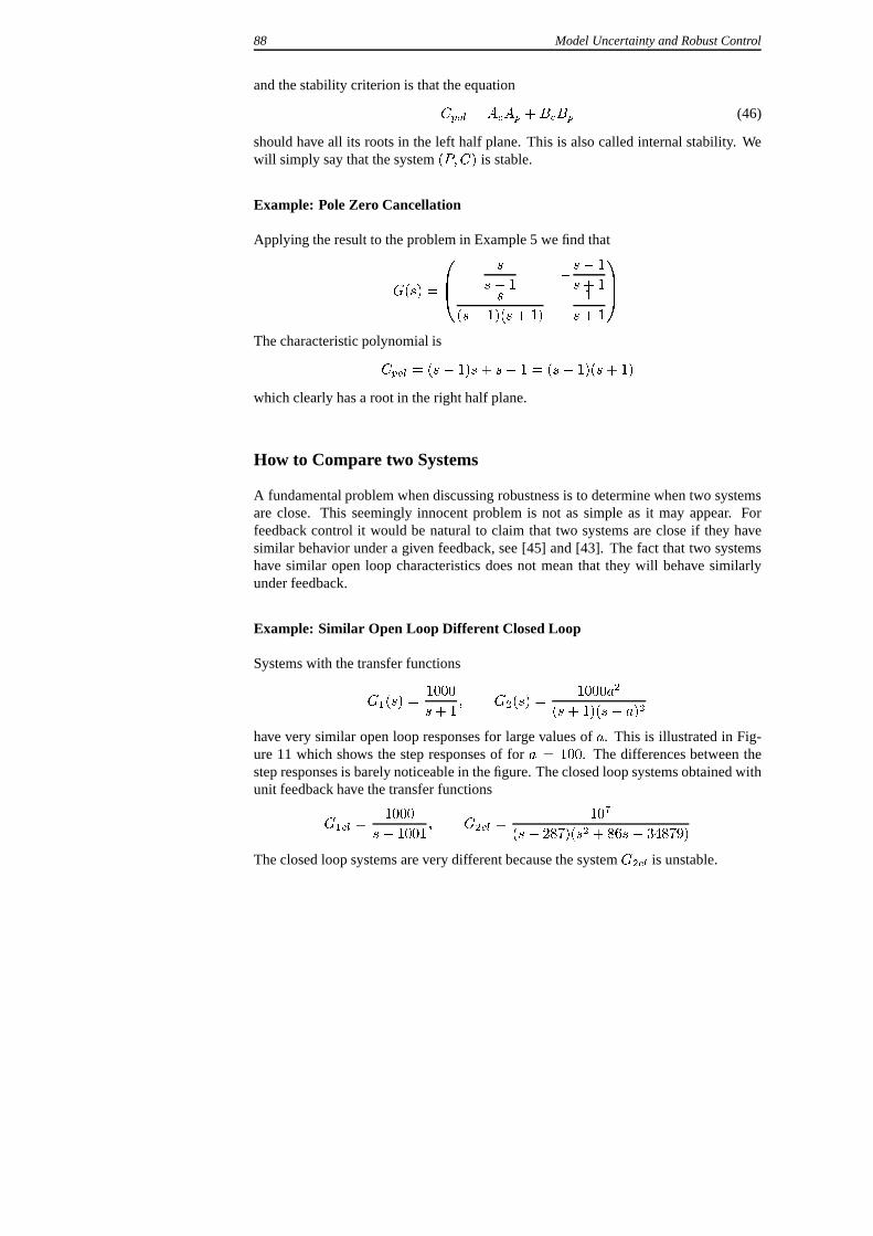
Example: Similar Open Loop Different Closed Loop

Systems with the transfer functions

G1(s) =1000

s+ 1; G2(s) =

1000a2

(s+ 1)(s+ a)2

have very similar open loop responses for large values ofa. This is illustrated in Fig-ure 11 which shows the step responses of fora = 100. The differences between thestep responses is barely noticeable in the figure. The closed loop systems obtained withunit feedback have the transfer functions

G1cl =1000

s+ 1001; G2cl =

107

(s� 287)(s2 + 86s+ 34879)

The closed loop systems are very different because the systemG2cl is unstable.


0 1 2 3 4 5 6 7 80

200

400

600

800

1000

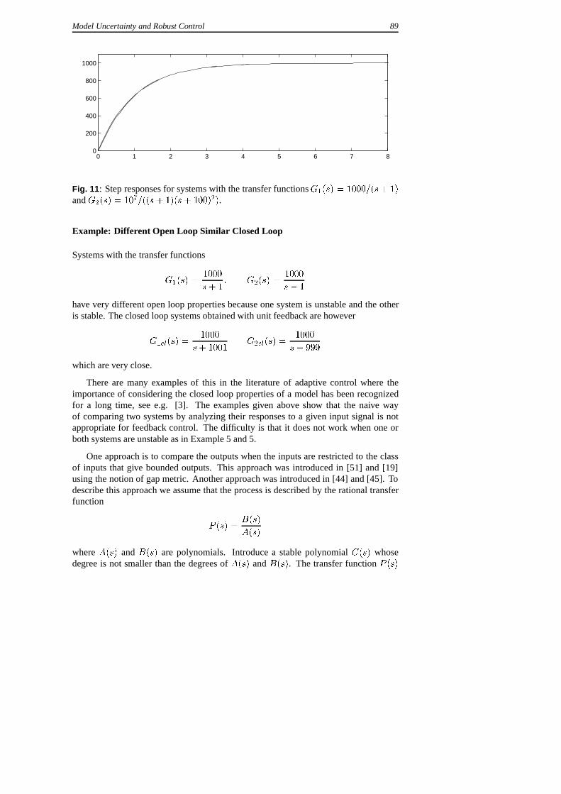
Fig. 11 : Step responses for systems with the transfer functionsG1(s) = 1000=(s+ 1)

andG2(s) = 107=((s+ 1)(s+ 100)2).

Example: Different Open Loop Similar Closed Loop

Systems with the transfer functions

G1(s) =1000

s+ 1; G2(s) =

1000

s� 1

have very different open loop properties because one system is unstable and the otheris stable. The closed loop systems obtained with unit feedback are however

G1cl(s) =1000

s+ 1001G2cl(s) =

1000

s+ 999

which are very close.

There are many examples of this in the literature of adaptive control where theimportance of considering the closed loop properties of a model has been recognizedfor a long time, see e.g. [3]. The examples given above show that the naive wayof comparing two systems by analyzing their responses to a given input signal is notappropriate for feedback control. The difficulty is that it does not work when one orboth systems are unstable as in Example 5 and 5.

One approach is to compare the outputs when the inputs are restricted to the classof inputs that give bounded outputs. This approach was introduced in [51] and [19]using the notion of gap metric. Another approach was introduced in [44] and [45]. Todescribe this approach we assume that the process is described by the rational transferfunction

P (s) =B(s)

A(s)

whereA(s) andB(s) are polynomials. Introduce a stable polynomialC(s) whosedegree is not smaller than the degrees ofA(s) andB(s). The transfer functionP (s)


can then be written as

P (s) =B(s)=C(s)

A(s)=C(s)=

D(s)

N(s)(47)

Vidyasagar proposed to compare two systems by comparing the stable rational transferfunctionsD andN . This is called the graph metric. A difficulty was that the graphmetric was difficult to compute.

Coprime Factorization

The polynomialC in (47) can be chosen in many different ways. We will now discussa convenient choice.

We start by introducing a suitable concept. Two rational functionsD andN arecalled coprime if there exist rational functionsX andY which satisfy the equation

XD + Y N = 1

The condition for coprimeness is essentially thatD(s) andN(s) do not have any com-mon factors. The functionsD(s) andN(s) will now be chosen so that

DD� +NN� = 1 (48)

where we have used the notationD�(s) = D(�s). A factorization (47) ofP whereNandD satisfy (48) is called a normalized coprime factorization ofP . Such a factoriza-tion the polynomialsA andB in (47) do not have common factors.

5.1 Vinnicombe’s Metric

A very nice solution to the problem of comparing two systems that is appropriate forfeedback was given by Vinnicombe, see [46] and [48]. Consider two systems with thenormalized coprime factorizations

P1 =D1

N1

P2 =D2

N2

To compare the systems it must be required that

1

2��arg

�(N1N

�

2+D1D

�

2) = 0 (49)

where� is the Nyquist contour. In the polynomial representation this condition impliesthat

1

2��arg

�(B1B

�

2+A1A

�

2) = degA2 (50)


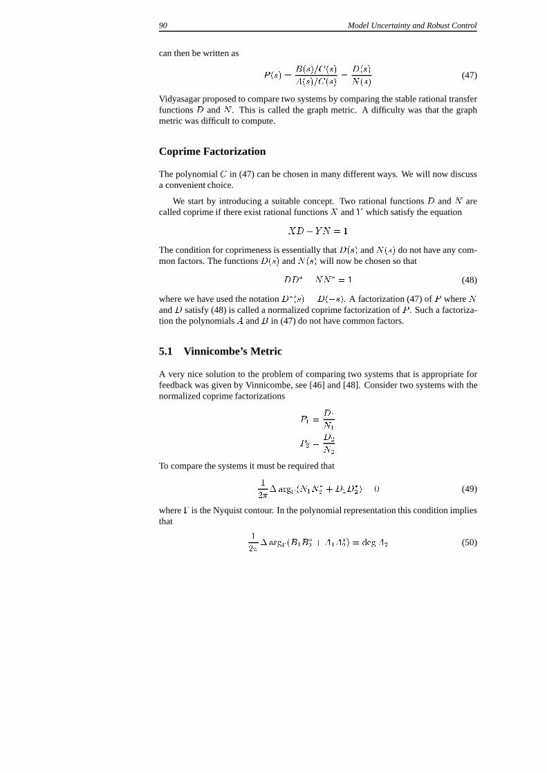
Fig. 12 : Geometric interpretation of the Vinnicombe metric.

If the winding number constraint is satisfied the distance between the systems is definedas

Æ�(P1; P2) = sup!

jP1(i!)� P2(i!)jp(1 + jP1(i!)j2)(1 + jP2(i!)j2)

(51)

We havejÆ�(P1; P2)j � 1. If the winding number condition is not satisfied the distanceis defined asÆ� = 1. Vinnicombe showed thatÆ� is a metric and he called it the�-gapmetric.

Geometric Interpretation

Vinnicombe’s metric is easy to compute and it also has a very nice geometric interpre-tation. The expression

d =jP1 � P2jp

(1 + jP1j2)(1 + jP2j2)

can be interpreted graphically as follows. LetP1 andP2 be two complex numbers. TheRiemann sphere is located above the complex plane. It has diameter 1 and its south poleis at the origin of the complex plane. Points in the complex plane are projected onto thesphere by a line through the point and the north pole, see Figure 12. LetR1 andR2 bethe projections ofP1 andP2 on the Riemann sphere. The numberd is then the shortestchordal distance between the pointsR1 andR2, see Figure 12.


��

�C

ND

�N�D

d v z x

u

n

y

w1 w2

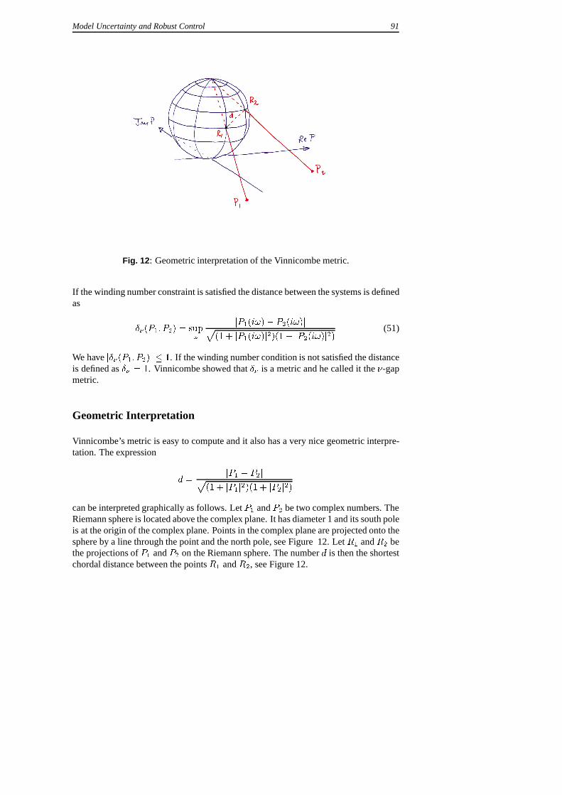
Fig. 13 : Block diagram of a process with coprime factor uncertainty and a controller.

Coprime Factor Uncertainty

Classical sensitivity results such as (8) were obtained based on additive perturbations.The systemP was perturbed toP +�P where�P is a stable transfer function. Thesetypes of perturbations are not well suited to deal with feedback systems as is illustratedby Example 5. A more sophisticated way to describe perturbations are required forthis. The development of the metrics for systems gave good insight into what should bedone. Uncertainty will be described in terms of the normalized coprime factorizationof a system. Consider a system described by

P +�P =N +�N

D +�D= ND�1 = D�1N (52)

whereN andD is a normalized coprime factorization ofP and the perturbations�Nand�Dare stable proper transfer functions. Figure 13 shows a block diagram of theclosed loop system with a the perturbed plant.

We will now investigate how large the perturbations can be without violating thestability condition. For the system in Figure 13 we have

z =D�1

1 + PCw1 �

D�1C

1 + PCw2 = D�1

�1

1 + PC� C

1 + PC

��w1

w2

�

and �w1

w2

�=

��D

�N

�z

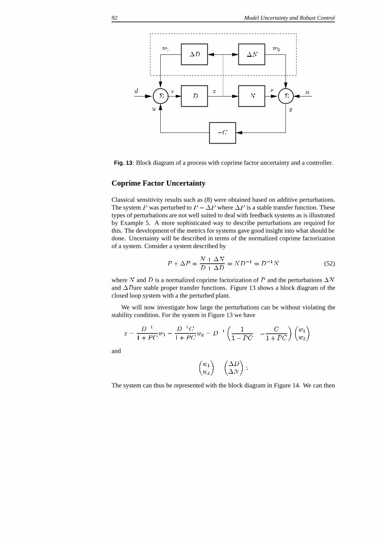
The system can thus be represented with the block diagram in Figure 14. We can then


�D, �N

P; C

w z

Fig. 14 : Simplification of the block diagram in Figure 13.

invoke the small gain theorem and conclude that the perturbed system will be stable ifthe loop gain is less than one, see [14]. Hence

��N�D

� 1

D�1

�1

1 + PC� C

1 + PC

� 1

< 1 (53)

This condition can be simplified if we use the fact thatN andD is a normalized coprimefactorization. This gives

D�1

�1

1 + PC� C

1 + PC

� 1

=

�D

N

�D�1

�1

1 + PC� C

1 + PC

� 1

�I

P

��1

1 + PC� C

1 + PC

� 1

= kG(P;C)k1

whereG(P;C) denotes the system matrix

G(P;C) =

0B@

1

1 + PC� C

1 + PCC

1 + PC� PC

1 + PC

1CA (54)

Introducing

(P;C) = sup!kG(P (i!); C(i!))k1 (55)

we thus find that the closed loop system is stable for all normalized coprime perturba-tions�D and�N such that

��N�D

� 1

<1

(56)


This equation is a natural generalization of Equation (8) in classical control theory.Notice that since the systems have one input and one output we have

jG(P;C)j = ��G(P;C) =

p(1 + jCj2)(1 + jP j2)

j1 + PCj (57)

and Equation (55) can thus be written

(P;C) = sup!

p(1 + jC(i!)j2)(1 + jP (i!)j2)

j1 + P (i!)C(i!)j (58)

H1-Loop Shaping

The goal ofH1 is to design control systems that are insensitive to model uncertainty.It follows from Equations (55) and (56) that this can be accomplished by finding acontrollerC that gives a stable closed loop system and minimizes theH1 norm of thetransfer functionG(P;C) given by Equation eq:gmatrix. It follows from Equation (56)that such a design permits the largest deviation of the normalized coprime deviations.

It is interesting to observe that the transfer functionG also describes the signaltransmission from the disturbancesd andn to v andx in Figure 2. A robust controllerobtained in this way will also attenuate the disturbances very well.

A state-space solution to theH1 control problem was given in [17]. A loop shapingdesign procedure was developed in [34] and [35].

Frequency Weighting

In the design procedure presented in [35] it is also possible to introduce a frequencyweightingW as a design parameter. TheH1 control problem for the processP 0 =PW is then solve giving the controllerC 0. The controller for the processP is thenC.In this way it is possible to obtain controller that have high gain at specified frequencyranges and high frequency roll off.

Generalized Stability Margin

A generalization of the classical stability margin was also introduced in [34]. For aclosed loop system consisting of the processP and the controllerC such that the closedloop system we define the generalized stability margin as

b(P;C) =

8<:1

if (P;C) is stable;

0 otherwise(59)


Notice that the generalized stability margin takes values between 0 and 1. The marginis 0 if the system is unstable. A value close to one indicates a good margin of stability.Reasonable practical values of the margin are in the range of1=3 to 1=5.

TheH1-loop shaping in [34] gives a controller that maximizes the stability margingiving

bopt = supC

b(P;C) (60)

Vinnicombe’s Theorems

A number of interesting theorems that relate model uncertainty to robustness have beenderived in [47] and [48]. These results, which can be seen as the natural conclusion ofthe work that began in [50], give very nice relations between robust control and modeluncertainty. Vinnicombe has proven the following results.

Proposition 1

Consider a nominal processesP and a controllerC and a parameter�. Then the con-trollerC stabilizes all plantsP1 such thatÆv(P; P1) � �, if and only if b(P;C) > �.

Proposition 2

Given a nominal processP , a perturbed processP1 and a number� < bopt(P;C).Then(P1; C) is stable for all compensatorsC, such thatb(P1; C) > � if and only ifÆ(P; P1) � �.

The first proposition tells that a controllerC designed for processP with a general-ized stability margin greater than� will stabilize all processesP1 in a Æv environmentof P provided thatÆv(P; P1) < �.

Proofs of these theorems are given in [48]. Vinnicombe has actually given sharperresults which only requires the inequalities to hold pointwise for each frequency.

Connections to the Classical Control Theory

TheH1-loop shaping cannot be directly related to the classical robustness criteria.The classical robustness criteria such asMt andMs depend only on the loop transferfunctionL = PC. But the generalized stability marginb(P;C) and the generalizedsensitivity (P;C) depend on bothP andC. The generalized stability margin willtherefore change if the process transfer function is multiplied by a constant and thecontroller transfer function is divided by the same number. One reason for this is thatthe criterion (57) implicitly assumes that the disturbances` andn have equal weight.This is a reasonable assumption if sufficient information about the disturbances are


available but very often we do not have this information. One possibility to formulatethe design problem in this case is to choose the most favorable disturbance relation.This can be done by introducing a weighting of the disturbances. LetP 0 = PW be theweighted process letCW�1 be the weighted controllerCW�1. We have

L0 = P 0C 0 = PC = L

The loop transfer function is invariant toW . The generalized sensitivity becomes

(P 0; C 0) = sup!

p(1 + jC(i!)W�1(i!)j2)(1 + jP (i!)W (i!)j2)

j1 + P (i!)C(i!)j

A straightforward calculation shows that 0 is minimized for the weight

W =pjCj=jP j

see [37]. This weight we get the following expression for the weighted sensitivity

� = sup!(jS(i!)j+ jT (i!)j) (61)

Notice that the weighted � only depends on the loop transfer functionL = PC.

Using the weighted sensitivity function we thus obtain an interesting connectionbetweenH1-loop shaping and classical robustness theory. The number " defined byEquation (55) and Equation (58) is a natural generalization of the maximaMs, Mt ofthe sensitivity function and the complementary sensitivity. It is useful to introduce acombined sensitivityM by requiring that bothMs andMt should at most be equalto M . The combined sensitivity implies that the Nyquist curve of the loop transferfunction is outside a circle with diameter on�

�M + 1

M � 1;�M � 1

M + 1

�The following inequalities are shown

2M � 1 < < 2M

2< M <

+ 1

2

in [37] where also sharper inequalities are presented.

The generalized stability marginb is also a natural generalization of the classicalstability marginAm. There are however some scale changes. The normal stability mar-gin takes values between 1 and1 while the generalized stability margin takes valuesbetween zero and one. To get compatibility the classical stability margin should beredefined as the distance between the critical point and the intersection of the Nyquistcurve with the negative real axis. Hence

A�m = 1� 1

Am


References

[1] K. J. Åström. Limitations on control system performance.European Journal ofControl, 6:1–19, 2000.

[2] Karl Johan Åström. Limitations on control system performance. InEuropeanControl Conference, Brussels, Belgium, July 1997.

[3] Karl Johan Åström and Björn Wittenmark.Adaptive Control. Addison-Wesley,Reading, Massachusetts, second edition, 1995.

[4] Karl Johan Åström and Björn Wittenmark.Computer-Controlled Systems. Pren-tice Hall, third edition, 1997.

[5] M. Athans and P. L. Falb.Optimal Control. McGraw-Hill, New York, 1966.

[6] T. Basar and P. Bernhard.H1-Optimal control and related minimax design prob-lems - A Dynamic game approach. Birkhauser, Boston, 1991.

[7] R. Bellman. Dynamic Programming. Princeton University Press, New Jersey,1957.

[8] R. Bellman, I. Glicksberg, and O. A. Gross. Some aspects of the mathematicaltheory of control processes. Technical Report R-313, The RAND Corporation,Santa Monica, Calif., 1958.

[9] H. S. Black. Stabilized feedback amplifiers.Bell System Technical Journal, 13:1–18, 1934.

[10] H. W. Bode. Relations between attenuation and phase in feedback amplifier de-sign. Bell System Technical Journal, 19:421–454, 1940.

[11] H. W. Bode. Network Analysis and Feedback Amplifier Design. Van Nostrand,New York, 1945.

[12] R. Clarke, J. J. Burken, J. T. Bosworth, and Bauer J.E. X-29 flight control system- Lessons learned.International Journal of Control, 59(1):199–219, 1994.

[13] J. C. Clegg. A nonlinear integrator for servomechanis.Trans. AIEE Part II, 77:41–42, 1958.

[14] C. A. Desoer and M. Vidyasagar.Feedback Systems: Input-Output Properties.Academic Press, New York, 1975.

[15] J. C. Doyle. Guaranteed margins for LQG regulators. AC-23:756–757, 1978.

[16] J. C. Doyle, B. A. Francis, and A. R. Tannenbaum.Feedback control theory.Macmillan, New York, 1992.

[17] J. C. Doyle, K. Glover, P.P Khargonekar, and B. A. Francis. State-space solutionsto standardh2 andH1 control problems. AC-34:831–847, 1989.


[18] J. C. Doyle and G. Stein. Multivariable feedback design: Concepts for a classi-cal/modern synthesis. AC-26:4–16, 1981.

[19] A. K. El-Sakkary. The gap metric: Robustness of stabilization of feedback sys-tems. AC-26:240–247, 1985.

[20] Gene F. Franklin, J. David Powell, and Abbas Emami-Naeini.Feedback Controlof Dynamic Systems. Addison-Wesley, third edition, 1994.

[21] Michael Green and D. J. N. Limebeer.Linear Robust Control. Prentice Hall,Englewood Cliffs, N.J., 1995.

[22] A. C. Hall. Application of circuit theory to the design of servomechanisms.Jour-nal of the Franklin Institute, 242:279–307, 1946.

[23] J. W. Helton and O. Merino.Classical control usingH1 Methods. SIAM,Philadelphia, 1999.

[24] I. M. Horowitz. Synthesis of Feedback Systems. Academic Press, New York, 1963.

[25] I. M. Horowitz and U. Shaked. Superiority of transfer function over state-variablemethods in linear time-invariant feedback system design. AC-20:84–97, 1975.

[26] Isac M. Horowitz.Quantitative Feedbac Design Theory (QFT). QFT Publications,Boulder, Colorado, 1993.

[27] H. M. James, N. B. Nichols, and R. S. Phillips.Theory of Servomechanisms. McGraw-Hill, New York, 1947.

[28] R. E. Kalman. A new approach to linear filtering and prediction problems.Trans-actions of the ASME, 82D:35–45, march.

[29] R. E. Kalman. Contributions to the theory of optimal control.Boletin de la So-ciedad Matématica Mexicana, 5:102–119, 1960.

[30] R. E. Kalman. When is a linear control system optimal?Trans. ASME Ser. D: J.Basic Eng., 86:1–10, March 1964.

[31] R. E. Kalman and R. S. Bucy. New results in linear filtering and prediction theory.Trans ASME (J. Basic Engineering), 83 D:95–108, 1961.

[32] R. E. Kalman, Y. Ho, and K. S. Narendra.Controllability of Linear DynamicalSystems, volume 1 ofContributions to Differential Equations. John Wiley & Sons,Inc., New York, 1963.

[33] Richard E. Klein. Using bicycles to teach system dynamics.IEEE Control SystemsMagazine, CSM:4–9, April 1986.

[34] D.C. MacFarlane and K. Glover.Robust controller design using normalized co-prime factor plant descriptions. Springer, New York, 1990.


[35] D.C. MacFarlane and K. Glover. A loop shaping design procedure usingH1-synthesis. AC-37:759–769, 1992.

[36] H. Nyquist. Regeneration theory.Bell System Technical Journal, 11:126–147,1932.

[37] H. Panagopoulos and K. J. Åström. PID control design andH1 loop shapingdesign of PI controllers based on non-convex optimization. InProceedings 1999IEEE Int. Conf. Control Applications and the Symp. Computer Aided Control Sys-tems Design (CCA’99&CACSD’99), Kohala Coast, Hawaii, August 1999.

[38] L. Pernebo. An algebraic theory for the design of controllers for linear multivari-able system - Part I: Structure matrices and feedforward design. AC-26:171–182,1981.

[39] L. Pernebo. An algebraic theory for the design of controllers for linear multivari-able system - Part II: Feeback realizations and feedback design. AC-26:173–194,1981.

[40] L. S. Pontryagin, V. G. Boltyanskii, R. V. Gamkrelidze, and E. F. Mischenko.TheMathematical Theory of Optimal Processes. John Wiley, New York, 1962.

[41] W. L. Rogers and D. J. Collins. X-29H1 controller synthesis.Journal of Guid-ance Control and Dynamics, 15(4):962–967, 1992.

[42] M. G. Safonov and M. Athans. Gain and phase margins for multiloop lqg regula-tors. AC-22:173–179, 1977.

[43] R. Skelton. Model error concepts in control design.International Journal ofControl., 49:1725–1753, 1989.

[44] M Vidyasagar. The graph metric for unstable plants and robustness estimates forfeedback stability. AC-29:403–417, 1984.

[45] Mathukumalli Vidyasagar.Control System Synthesis: A Factorization Approach.MIT Press, Cambridge, Massachusetts, 1985.

[46] G. Vinnicombe. Frequency domain uncertainty and the graph topology. AC-38:1371–1383, 1993.

[47] G. Vinnicombe. The robustness of feedback systems with bounded complexitycontrollers. AC-41:795–803, 1996.

[48] G. Vinnicombe. Uncertainty and Feedback:H1 loop-shaping and the�-gapmetric. Imperial College Press, London, 1999.

[49] G. Zames. Feedback and optimal sensitivity: Model reference transformations,multiplicative seminorms, and approximative inverse. AC-26(2):301–320, 1981.

[50] G. Zames. Feedback and optimal sensitivity: Model reference transformations,multiplicative seminorms, and approximative inverses. AC-26:301–320, 1981.


[51] G. Zames and A. K. El-Sakkary. Unstable systems and feedback: The gap metric.In Proc. Allerton Conference, pages 380–385, 1980.

[52] J. C. Zhou, J. C. Doyle, and K. Glover.Robust and optimal control. Prentice Hall,New Jersey, 1996.

[53] R. L. Bagley and R. A. Calico. Fractional-order state equations for the control ofviscoelastic damped structures. J. Guidance, Control and Dynamics (14) 304-311,1991.

[54] A. Oustaloup. La Commande CRONE. Hermes, Edition CNRS, Paris, France,1991.

[55] A. Oustaloup. La Derivation Non Entiere: Theorie, Synthese et Applications.Hermes, Paris, France, 1995.

[56] I. Podlubny. Fractional Differential Equations. Academic Press, NY, 1999a.

[57] I. Podlubny. Fractional-order systems and PID controllers. IEEE Trans AC-44,208–214, 1999.

Documents

Model Uncertainty and Robust Control Model Uncertainty and Robust Control transfer functions or frequency responses. It was very natural to capture uncertainty in terms of deviations