MODEL SSA 7-6-Running-Model.v 1.3 - Coastal SAF · Version 1.3 21 February 2010 Page 1 System Formulation Part 2: Running the model ExtendSim Model with input and ouput The SPICOSA

Version 1.3 21 February 2010 Page 1

System Formulation Part 2: Running the model ExtendSim Model with input and ouput

The SPICOSA SSA 7.6, Søndeledfjorden, Norway

Version 1.3 (21 February 2010)

Erlend Moksness1, Jakob Gjøsæter1, Inga Wigdahl Kaspersen2, Eirik Mikkelsen3, Håkan T. Sandersen5 and Jon Helge Vølstad1

1) Institute of Marine Research, Flødevigen Marine Research Station, 4817 His, Norway 2) University of Tromsø, Department of Economics and Management, 9037 Tromsø, Norway

3) Norut AS, Postboks 6434 Forskningsparken, 9294 Tromsø, Norway 4) Institute of Marine Research, 5817 Bergen, Norway

Bodø University College, Dep. of Social Science, 8049 Bodø, Norway

ExtendSim Model developer

Guillaume Lagaillarde, 1point2, France


Table of Content Page 1. What you need ...................................................................................................... 3 2. General description ............................................................................................... 4 2.1 Environmental component (NC) ................................................................................. 4 2.2 Social component (SC) ................................................................................................ 6 2.3 Economic component (EC) .......................................................................................... 7 3. Changing Input parameters ................................................................................... 8 3.1 General ........................................................................................................................ 8 3.2 Environmental component (NC) ................................................................................. 8 3.3 Social component (SC) ................................................................................................ 9 3.4 Economic component (EC) ........................................................................................ 11 3.5 Indicators .................................................................................................................. 12 4. Regulations and scenarios ................................................................................... 13 5. Output and export of data ................................................................................... 16 5.1 General ...................................................................................................................... 16 5.2 Environmental (cod population) ............................................................................... 16 5.3 Economic ................................................................................................................... 18 5.4 Export of data to MS Excel ........................................................................................ 19 6. Adopting the model to other local cod stocks and fjord systems ......................... 21 7 Calculations ......................................................................................................... 21 7.1 Ecosystem (Cod population) ..................................................................................... 21 7.1.1. Estimating annual recruitment (Number of 0‐group cod) .................................... 21 7.1.2. Estimating cohort sizes over the chosen time frame ........................................... 21 7.1.3. Estimating survival from 0‐group to 1‐group cod ................................................. 22 7.2 Social ......................................................................................................................... 24 7.3 Economic ................................................................................................................... 25


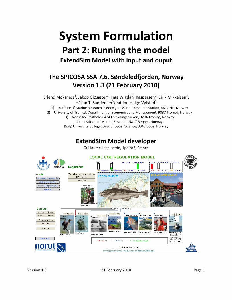
1. What you need Make sure you have the following files in the same folder:

‐ The ExtendSim Model ‐ CodFish.lix ‐ ExportedData.xls

It is possible to set simulation duration up to 50 years. You can run up to 100 simulations. First select “Simulation setup” from the “Run” menu.

Secondly enter the number years for the run (maximum 50 years) and the total number of simulations (“Runs”) (unlimited). Then you can select “Run simulation” from the “Run” menu.


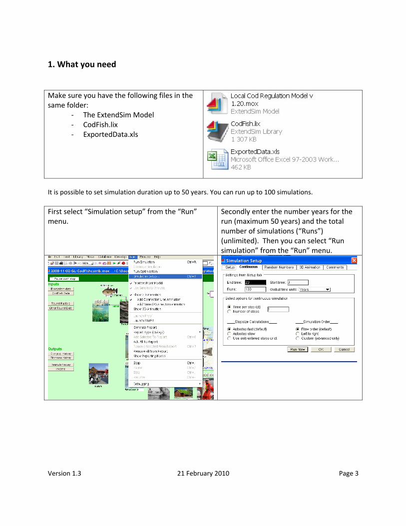
2. General description The model consists of several tables that contain input and output data. The different tables can be viewed by selecting the codfish model from the Database menu, as showed in the figure to the right.

2.1 Environmental component (NC) The ecosystem model is a demographic model that projects the abundance of the coastal cod (Gadus morhua) population in SSA 7.6 (Søndeledfjorden, Norway) in numbers by age (0 ‐ 10 years age groups) forward in time.

• The model is running with yearly time‐steps over a period of 1‐50 years. • Recruitment of 0‐group cod are randomly picked by the model from a distribution of historical

data. • The total population size and the strength of the different year‐classes of cod is a function of

natural predators (as birds and mammals) and fishing mortality (caused by tourists and commercial) and other human activities (Eco‐tourists etc).

• The cod spawning stock (SS) consists of age‐groups 4‐10. • The default fishable stock consists of age‐groups 2‐10, however, will vary between user groups • Several policy instruments influence the dynamics of the cod population: TAC (total allowable

catch on each year‐class per year), amount of bottom habitat occupied by marinas, and the number of predators (birds and mammals) which can be controlled by hunting.

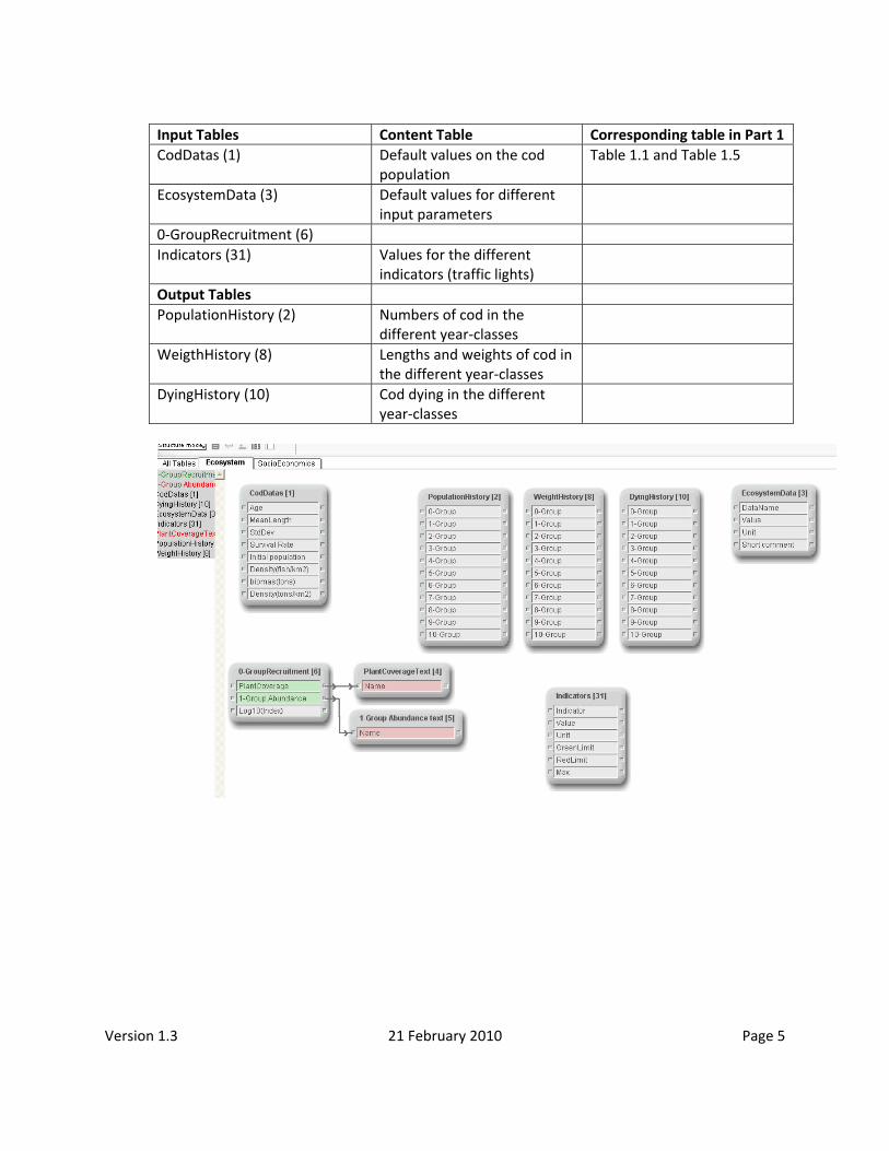
In the following tables and figures you can view the different tables used in the ecosystem component in the model.


Input Tables Content Table Corresponding table in Part 1 CodDatas (1) Default values on the cod

population Table 1.1 and Table 1.5

EcosystemData (3) Default values for different input parameters

0‐GroupRecruitment (6) Indicators (31) Values for the different

indicators (traffic lights)

Output Tables PopulationHistory (2) Numbers of cod in the

different year‐classes

WeigthHistory (8) Lengths and weights of cod in the different year‐classes

DyingHistory (10) Cod dying in the different year‐classes


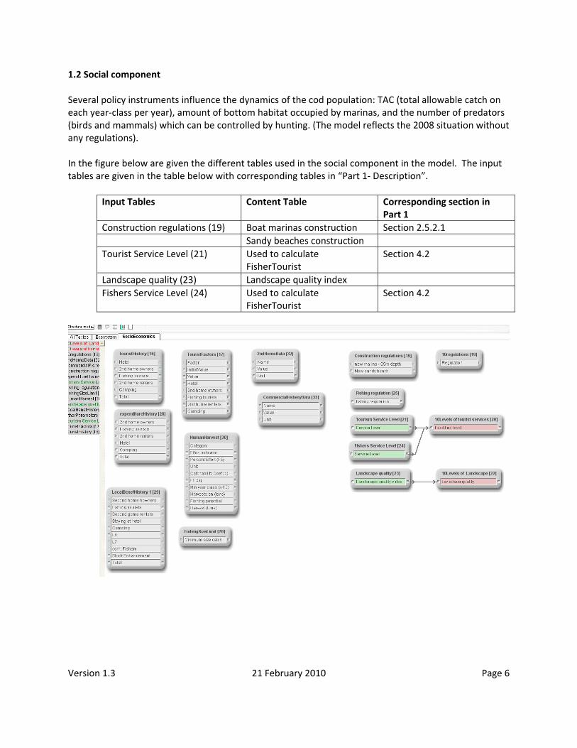
1.2 Social component Several policy instruments influence the dynamics of the cod population: TAC (total allowable catch on each year‐class per year), amount of bottom habitat occupied by marinas, and the number of predators (birds and mammals) which can be controlled by hunting. (The model reflects the 2008 situation without any regulations). In the figure below are given the different tables used in the social component in the model. The input tables are given in the table below with corresponding tables in “Part 1‐ Description”.

Input Tables Content Table Corresponding section in

Part 1 Construction regulations (19) Boat marinas construction Section 2.5.2.1 Sandy beaches construction Tourist Service Level (21) Used to calculate

FisherTourist Section 4.2

Landscape quality (23) Landscape quality index Fishers Service Level (24) Used to calculate

FisherTourist Section 4.2


1.3 Economic component The main aim of economic component is to estimate (net) local economic benefits from tourism in the Søndeledfjord area. This is set equal to Risør municipality in our case. The economic benefits/costs related to tourism that we consider come from 1) expenditures from tourists visiting the area (except 2nd home building and maintenance), and multiplicator effects of those expenditures, 2) the building and maintenance of 2nd homes + multiplicator effects, 3) changed income in commercial fishery due to changes in the coastal cod stock due to tourism (fishing + habitat changes), and 4) net local costs of coastal cod stock enhancement. In the figure below are given the different tables used in the economic component in the model. The input and output tables are given in the table below with corresponding tables in “Part 1‐ Description”.

Input Tables Content Table Corresponding table in Part 1 Touristfactors (17) Contain default values of

parameters Table 3.3

OtherParameter (27) Contain default values of parameters

Table 3.4

HumanHarvest (30) Contain default values of parameters

Table 1.3

CommersialFisheryData (31) Contain default price for cod Chapter 3.3 2ndHomeData (32) Default economical

parameters Chapter 3.2

Output Tables TouristHistory (16) Number of tourist‐days in the

different categories

ExpenditureHistory (28) Cost in the different categories

LocalBenefHistory (29) Income from the different categories


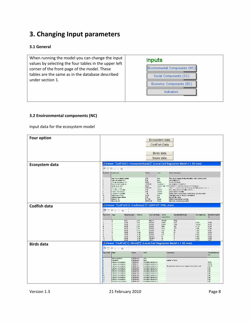
3. Changing Input parameters 3.1 General When running the model you can change the input values by selecting the four tables in the upper left corner of the front page of the model. These tables are the same as in the database described under section 1.

3.2 Environmental components (NC) Input data for the ecosystem model Four option

Ecosystem data

Codfish data

Birds data


Seals data

3.3 Social component (SC) Two option

Eel fishers

Net fishing data

In addition the fishing effort, coefficients in the Schaffer model and minimum fish size (represented by minimum year‐class) (Table 1.3 in the document “Part 1: ExtendSim Model description”) can be changed Extend input table “HumanHavest (30)”.


Table 1.3 in the document “Part 1: ExtendSim Model description”.


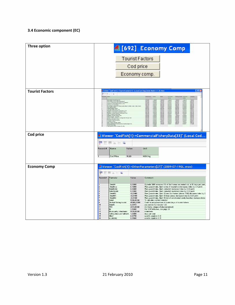
3.4 Economic component (EC) Three option

Tourist Factors

Cod price

Economy Comp


3.5 Indicators


4 Regulations and Scenarios Three options

Tourist fisher accommodation The standard is indicated by number of stars (1‐5 – worst to best), according to NHO’s (The Confederation of Norwegian Enterprises) classification system for fishing tourism accommodation, see http://www.fisketurisme.no). We assume that beds in premises with 5 stars are utilized 100% for the 180 day season. 1 star gives only 20% capacity utilization (36 days). Number of dedicated beds for tourist fishers can be changed.

MPA habitat Option 1: Non Option 2: No new sandy beaches Option 3: No new sandy beaches and marinas over depths less than 25 m

MPA cod Option 1: Non Option 2: No fishing during spawning period (3 months) with nets Option 3: No fishing during spawning period (3 months) with nets and hooks Option 4: No fishing of cod through the whole year with nets and trawl Option 5: No fishing of cod through the whole year with nets, trawl and hooks

Eel‐fishers The default number of eel fishers is set to 3.


2nd homes The present numbers of 2nd homes in the study area is 1523. Over the next years it might expand to nearly 2000. The effect of each 2nd home is that the available 0‐group cod habitat is reduced with 50m2.

Recreational fishers The numbers of recreational fishers are dependent of number of municipal inhabitants

Camping tourists The numbers of camping tourists are dependent on parameters given in the economical component.

Tourist fishers The present numbers of tourist fishers are dependent on the number of beds available and quality of the facilities

Commercial fishers The numbers of commercial fishers are are set directly.


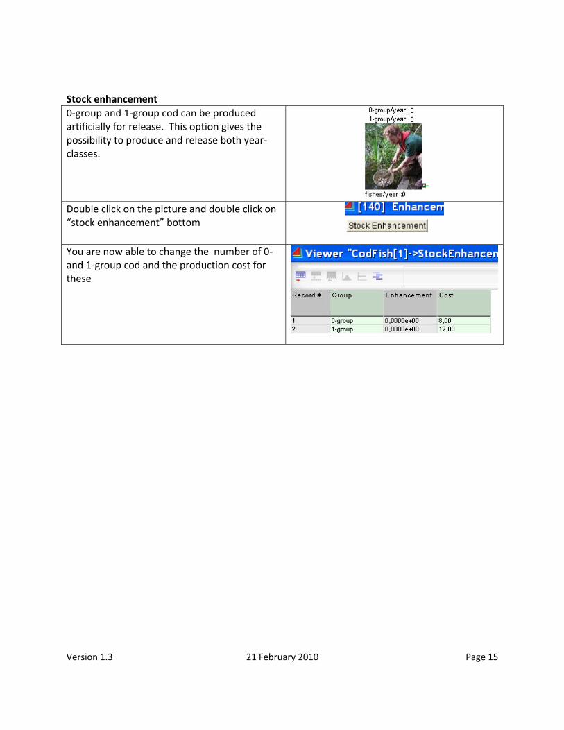
Stock enhancement 0‐group and 1‐group cod can be produced artificially for release. This option gives the possibility to produce and release both year‐classes.

Double click on the picture and double click on “stock enhancement” bottom

You are now able to change the number of 0‐ and 1‐group cod and the production cost for these


5. Output and export of data

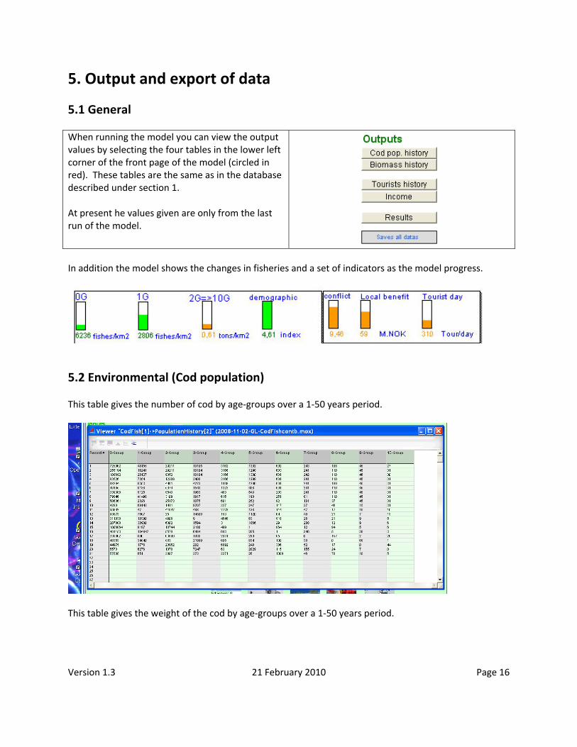
5.1 General When running the model you can view the output values by selecting the four tables in the lower left corner of the front page of the model (circled in red). These tables are the same as in the database described under section 1. At present he values given are only from the last run of the model.

In addition the model shows the changes in fisheries and a set of indicators as the model progress.

5.2 Environmental (Cod population) This table gives the number of cod by age‐groups over a 1‐50 years period.

This table gives the weight of the cod by age‐groups over a 1‐50 years period.


By choosing results the below figure will appear. The figure shows the average number (solid blue) and weight (solid red) of cod + the same values from the last run as stippled In addition the values for:

‐ Density 0‐1‐gr (number km‐2) ‐ Biomass (2‐10 yrs) (ton km‐2) ‐ Commercial fishing (2‐10 yrs) (ton km‐2) ‐ Conflict Factor ‐ Local income

are given below and present output values from the model.


5.3 Economic The results from the economic run will be displayed and exported similar to the ecosystem data (Not available yet) This table gives the number of person pr day (T0) over a time period (1‐50 years) selected. The same Table as TouristHistory in Databases. Corresponds to Table 3.3 and 3.5.

This table gives the income over 1‐50 years period.


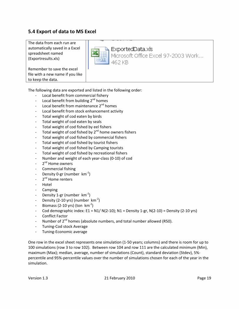
5.4 Export of data to MS Excel The data from each run are automatically saved in a Excel spreadsheet named (Exportresults.xls) Remember to save the excel file with a new name if you like to keep the data. The following data are exported and listed in the following order:

‐ Local benefit from commercial fishery ‐ Local benefit from building 2nd homes ‐ Local benefit from maintenance 2nd homes ‐ Local benefit from stock enhancement activity ‐ Total weight of cod eaten by birds ‐ Total weight of cod eaten by seals ‐ Total weight of cod fished by eel fishers ‐ Total weight of cod fished by 2nd home owners fishers ‐ Total weight of cod fished by commercial fishers ‐ Total weight of cod fished by tourist fishers ‐ Total weight of cod fished by Camping tourists ‐ Total weight of cod fished by recreational fishers ‐ Number and weight of each year‐class (0‐10) of cod ‐ 2nd Home owners ‐ Commercial fishing ‐ Density 0‐gr (number km‐2) ‐ 2nd Home renters ‐ Hotel ‐ Camping ‐ Density 1‐gr (number km‐2) ‐ Density (2‐10 yrs) (number km‐2) ‐ Biomass (2‐10 yrs) (ton km‐2) ‐ Cod demographic index: E1 = N1/ N(2‐10); N1 = Density 1‐gr, N(2‐10) = Density (2‐10 yrs) ‐ Conflict Factor ‐ Number of 2nd homes (absolute numbers, and total number allowed (R50). ‐ Tuning‐Cod stock Average ‐ Tuning‐Economic average

One row in the excel sheet represents one simulation (1‐50 years; columns) and there is room for up to 100 simulations (row 3 to row 102). Between row 104 and row 111 are the calculated minimum (Min), maximum (Max); median, average, number of simulations (Count), standard deviation (Stdev), 5%‐percentile and 95%‐percentile values over the number of simulations chosen for each of the year in the simulation.


This table explanation of content of the different sheets in the excel‐file “ExportedData.xls” Sheet name Content 1 Content 2 LocBenCommFishery Local benefit from commercial

fishery

LocBenConstruction Local benefit from building 2nd homes

LocBenMaintenance Local benefit from maintenance 2nd homes

LocBenStkEnhance Local benefit from stock enhancement activity

BirdsEating Total weight of cod eaten by birds SealsEating Total weight of cod eaten by seals EelFishersEating Total weight of cod fished by eel

fishers

SecondHEating Total weight of cod fished by 2nd home owners fishers

NetFishersEating Total weight of cod fished by commercial fishers

TouristFishersEating Total weight of cod fished by tourist fishers

CampinFishersEating Total weight of cod fished by Camping tourists

RecretationFishersEating Total weight of cod fished by recreational fishers

Group0 Number of fishes Biomass of fishes (kg) Group1 Number of fishes Biomass of fishes (kg) Group2 Number of fishes Biomass of fishes (kg) Group3 Number of fishes Biomass of fishes (kg) Group4 Number of fishes Biomass of fishes (kg) Group5 Number of fishes Biomass of fishes (kg) Group6 Number of fishes Biomass of fishes (kg) Group7 Number of fishes Biomass of fishes (kg) Group8 Number of fishes Biomass of fishes (kg) Group9 Number of fishes Biomass of fishes (kg) Group10 Number of fishes Biomass of fishes (kg) SecondHomeOwn Number of Touristdays Expenditure (NOK) Fishing Number of Touristdays; Fishing

tourists Expenditure (NOK)

SecondHomeRent Number of Touristdays Expenditure (NOK) Hotel Number of Touristdays; tourists

staying at hotels Expenditure (NOK)

Camping Number of Touristdays; Camping tourists

Expenditure (NOK)

0Gdensity 0‐group cod; density (number/km2)


1Gdensity 1‐group cod; density (number/km2)

2‐10Gdensity Sum of 2‐10 group cod; density (number/km2)

2‐10Gbiomass Sum of 2‐10 group cod biomass (kg)

DemogIndex Demographic Index = 0G/(2‐10G); 0G = Number of 0‐group cod; (2‐10G) sum of Number of 2‐10 group cod

ConflictFactor See Chapter 2.8 (Description document)

Number2ndHomes Total number of 2nd Homes Tuning‐Cod stock Average

Excel sheet to help in tuning the ecological component

Tuning‐Economic average

Excel sheet to help in tuning the economic component


6. Adopting the model to other local cod stocks and fjord systems The model can easily be adapted to other fjord systems and their cod stock. You have to change the parameters given chapter 2.

7 Calculations 7.1 Cod population 7.1.1 Estimating annual recruitment (Number of 0‐group cod) The left figure shows where the annual recruitment is calculated in the model and the right figure shows the content of the recruitment box. The abundance of the 0‐group cod in the population is modeled as a function of the area of suitable habitats (eelgrass etc; at present the default value is 1) for recruitment, the strength of the 1‐group cod and that the spawning stock (year‐classes 4‐10) consist of more than 100 cod.

7.1.2 Estimating cohort sizes over the chosen time frame The calculations in the ecosystem model take place in the block shown to the right. When open it the structure will be seen as below. Average numbers of code in the different year‐classes of cod are calculated in the different “multi average” boxes.


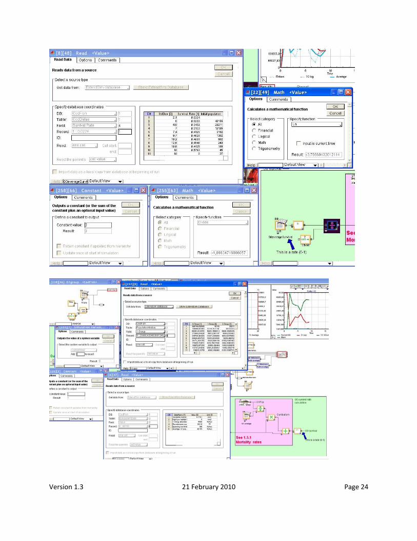
7.1.3 Estimating survival from 0‐group to 1‐group cod The mortality caused by 1‐group cod on the 0‐group cod can be changed by entering this input‐table and changes the value in the last line.

The survival from 0‐group cod to 1‐group cod are calculated in the three figures shown below.



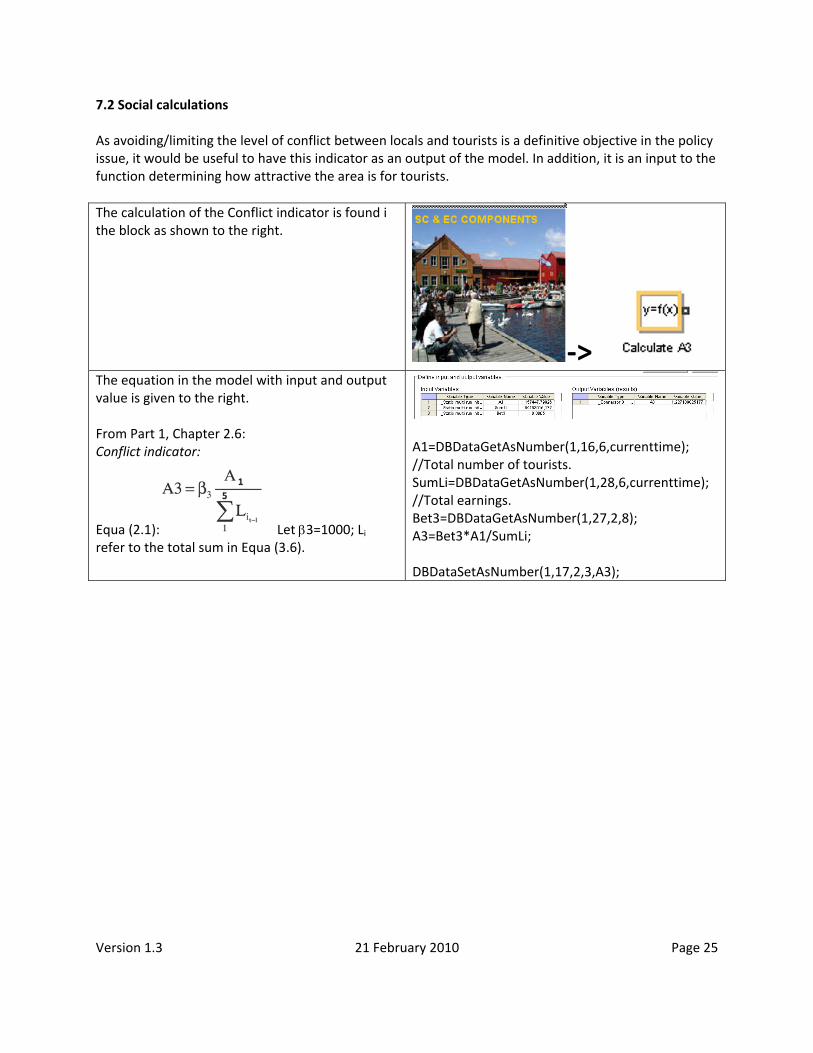
7.2 Social calculations As avoiding/limiting the level of conflict between locals and tourists is a definitive objective in the policy issue, it would be useful to have this indicator as an output of the model. In addition, it is an input to the function determining how attractive the area is for tourists. The calculation of the Conflict indicator is found i the block as shown to the right.

‐>

The equation in the model with input and output value is given to the right. From Part 1, Chapter 2.6: Conflict indicator:

Equa (2.1): Let β3=1000; Li refer to the total sum in Equa (3.6).

A1=DBDataGetAsNumber(1,16,6,currenttime); //Total number of tourists. SumLi=DBDataGetAsNumber(1,28,6,currenttime); //Total earnings. Bet3=DBDataGetAsNumber(1,27,2,8); A3=Bet3*A1/SumLi; DBDataSetAsNumber(1,17,2,3,A3);


7.3 Economic calculations The economic calculations take place in the bloc shown on the left. The different calculations are taken place in the blocs shown below

Calculate total number of tourists (Part 1, Table 3.2)

A1=5

ii 1

T=∑

Documents

MODEL SSA 7-6-Running-Model.v 1.3 - Coastal SAF · Version 1.3 21 February 2010 Page 1 System Formulation Part 2: Running the model ExtendSim Model with input and ouput The SPICOSA