Model selection and local geometry.

Robin J. EvansUniversity of Oxford

evans@stats.ox.ac.uk

December 6, 2019

Abstract

We consider problems in model selection caused by the geometry of models closeto their points of intersection. In some cases—including common classes of causal orgraphical models, as well as time series models—distinct models may nevertheless haveidentical tangent spaces. This has two immediate consequences: first, in order to ob-tain constant power to reject one model in favour of another we need local alternativehypotheses that decrease to the null at a slower rate than the usual parametric n−1/2

(typically we will require n−1/4 or slower); in other words, to distinguish between themodels we need large effect sizes or very large sample sizes. Second, we show that undereven weaker conditions on their tangent cones, models in these classes cannot be madesimultaneously convex by a reparameterization.

This shows that Bayesian network models, amongst others, cannot be learned directlywith a convex method similar to the graphical lasso. However, we are able to use ourresults to suggest methods for model selection that learn the tangent space directly,rather than the model itself. In particular, we give a generic algorithm for learningBayesian network models.

1 Introduction

Consider a class of probabilistic models Mi indexed by elements of some set i ∈ I, andsuppose that we have data from some distribution P ; model selection is the task of deducing,from the data, which Mi contains P . Typically there will be multiple such models, in whichcase one may appeal to parsimony or—if the model class is closed under intersection—selectthe smallest such model by inclusion.

There have been dramatic advancements in certain kinds of statistical model selection,including methods for working with large datasets and very high-dimensional problems (see,for example, Buhlmann and van de Geer, 2011). However, model selection in some settings ismore difficult; for example, selecting an optimal Bayesian network for discrete data is knownto be an NP-complete problem (Chickering, 1996). In this paper we consider why somemodel classes are so much harder to learn with than others. Taking a geometric approach, wefind that some classes contain models which are distinct but—in a sense that will be madeprecise—are locally very similar to one another. The task of distinguishing between themusing data is therefore fundamentally more difficult, both statistically and computationally.

Example 1.1. To illustrate the main idea in simple terms, consider a model space smoothlydescribed by a two dimensional parameter θ = (θ1, θ2)T ∈ R2, and with four submodels ofinterest:

M∅ : θ1 = θ2 = 0 M1 : θ2 = 0

M2 : θ1 = 0 M12 : unrestricted.

In a setting with independent data, we would expect to have statistical power sufficient todistinguish betweenM12 andM2 (i.e. to determine whether or not θ1 = 0) provided that the

1

arX

iv:1

801.

0836

4v4

[m

ath.

ST]

5 D

ec 2

019

O(δ2)

δ

(b)O(δ)

δ

(a)

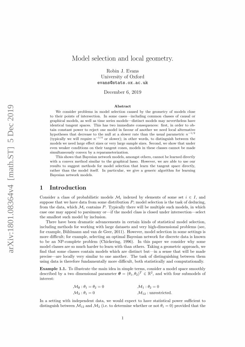
Figure 1: Illustration of model selection close to points of intersection. On the left, the modelsM1 and M2 (in blue and red respectively) have different tangent spaces, so the distancebetween them increases linearly as one moves away from the intersection. On the right, themodels M1 (in blue) and M′2 (in red) have the same tangent space at the intersection, sothey diverge only quadratically with distance from the intersection.

magnitude of θ1 is large compared to n−1/2, where n is the number of independent samplesavailable. We might also expect to be able to distinguish between M1 and M2 at the sameasymptotic rate; this is the picture in Figure 1(a), in which the distance between the twomodels is proportional to distance from their intersection M∅ =M1 ∩M2 (the constant ofproportionality being determined by the angle between the two models).

Suppose now that we define a model M′2 : ψ1 = 0, where ψ1 ≡ θ21 − θ2, and have to

select betweenM∅,M1,M′2,M12 (note that we still haveM∅ =M1∩M′2), as illustrated inFigure 1(b). Superficially, the task of choosing between these four models seems no differentto our first scenario, but in fact the models M1 and M′2 are locally linearly identical at thepoint of intersection ψ1 = θ2 = 0: that is, the tangent spaces of the two models at this pointare the same, so up to a linear approximation they are indistinguishable.

Models that overlap linearly in the manner above lead to two major consequences relatingto statistical power and computational efficiency. First, as illustrated in Figure 1(b), if M1

is correct the distance1 between the true parameter value (θ1, 0) and the closest point onM′2grows quadratically rather than linearly in θ1. Hence, while |θ1| = Ω(n−1/2) is sufficient togain power against M∅, one needs |θ1| = Ω(n−1/4) to ensure power2 against M′2. This ispotentially a very stringent condition indeed: if the effect size is halved, then we will need 16times the sample size to maintain power against the alternative model.

Second, if two models have the same tangent space then we cannot choose a parameteri-zation under which both models are convex sets. Note that in Figure 1(a) all four models areconvex, but in Figure 1(b) the model M′2 is not. If we reparameterize to make M′2 convex,then M1 will not be3. This prevents penalized methods such as the lasso being used in acomputationally efficient way.

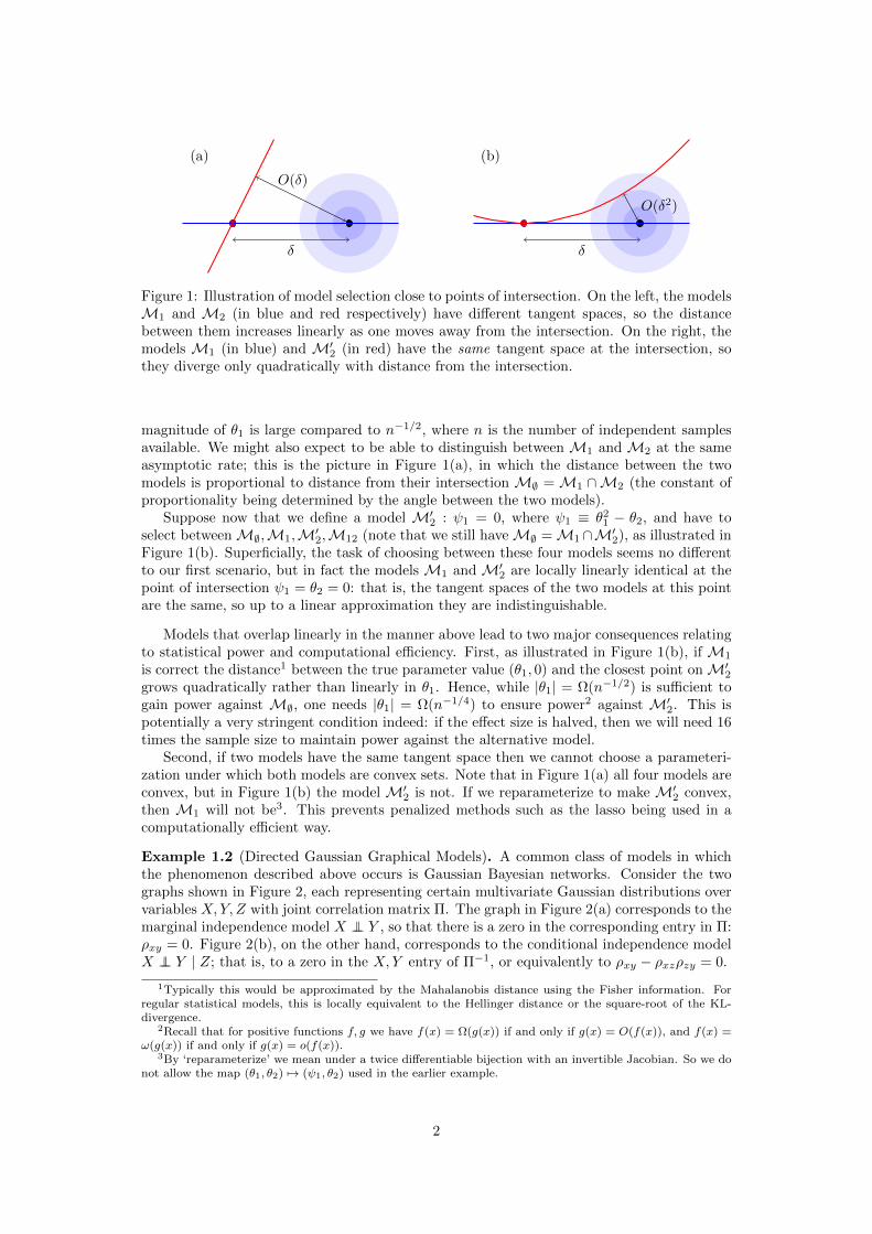
Example 1.2 (Directed Gaussian Graphical Models). A common class of models in whichthe phenomenon described above occurs is Gaussian Bayesian networks. Consider the twographs shown in Figure 2, each representing certain multivariate Gaussian distributions overvariables X,Y, Z with joint correlation matrix Π. The graph in Figure 2(a) corresponds to themarginal independence model X ⊥⊥ Y , so that there is a zero in the corresponding entry in Π:ρxy = 0. Figure 2(b), on the other hand, corresponds to the conditional independence modelX ⊥⊥ Y | Z; that is, to a zero in the X,Y entry of Π−1, or equivalently to ρxy − ρxzρzy = 0.

1Typically this would be approximated by the Mahalanobis distance using the Fisher information. Forregular statistical models, this is locally equivalent to the Hellinger distance or the square-root of the KL-divergence.

2Recall that for positive functions f, g we have f(x) = Ω(g(x)) if and only if g(x) = O(f(x)), and f(x) =ω(g(x)) if and only if g(x) = o(f(x)).

3By ‘reparameterize’ we mean under a twice differentiable bijection with an invertible Jacobian. So we donot allow the map (θ1, θ2) 7→ (ψ1, θ2) used in the earlier example.

2

X

Z

Y

(a)

X

Z

Y

(b)

Figure 2: Two Bayesian networks in which, for Gaussian random variables, the tangent spacesof the models are identical at some points of intersection.

The two models intersect along two further submodels: for example, if ρxz = 0 (so thatX ⊥⊥ Z), then ρxy = 0 if and only if ρxy − ρxzρzy = 0. The same thing happens if ρyz = 0(i.e. Y ⊥⊥ Z). When we are at the intersection between all these submodels—so ρxy = ρxz =ρyz = 0 and all variables are jointly independent—we find that the tangent spaces of thetwo original models are the same, giving rise to the phenomenon described above. Indeed,we will see that this arises whenever two models intersect along two or more such—suitablydistinct—further submodels (Theorem 3.1).

1.1 Background and Prior Work

Crudely speaking, there are two flavours of statistical model, and consequently two mainreasons for wishing to select one. The first, called substantive or explanatory, emphasizesthe use of models to explain underlying phenomena, and such models are sometimes viewedas approximations to an unknown scientific ‘ground truth’ (Cox, 1990; Skrondal and Rabe-Hesketh, 2004). The second kind, referred to as empirical or predictive, is mainly concernedwith predicting outcomes from future observations, generally assuming that such observationswill arise from the same population as previous data (Breiman, 2001). A discussion of thesetwo camps, together with some finer distinctions can be found in Cox (1990).

Our focus will primarily be on substantive models, in which case different models maylead to rather different practical conclusions, even if the probability distributions associatedwith them are ‘close’ in the sense observed above. The case of causal models such as thegraphs in Figure 2 is particularly stark: the reversal of an arrow will significantly affectour understanding of how a system will behave under an intervention. For interpolativeprediction—that is, with new data from the same population as the data used to learn themodel—such concerns are generally lessened: if two probability distributions are similar thenthey should give similar conclusions. However, the computational concerns we raise will affectmodel selection performed for whatever reason.

For Bayesian network (BN) models specifically, there has been a great deal of work dealingwith the problem of accurate learning from data. Chickering (1996) showed that the problemof finding the BN which maximizes a penalized likelihood criterion is NP-complete in the caseof discrete data with several common penalties. Uhler et al. (2013) give geometric proofs thatdirected Gaussian graphical models are, in a global sense, very hard to learn using sequentialindependence tests; this is because the volume of ‘unfaithful’ points that will mislead atleast one hypothesis test for a given sample size is very large, and in settings where thenumber of parameters is larger than the number of observations will overwhelm the model.Our approach is considerably simpler and is applicable to arbitrary model classes and modelselection procedures, but cannot make global statements about the model.

Shojaie and Michailidis (2010) provide a penalized method for learning sparse high-dimensional graphs, but they assume a known topological ordering for the variables in thegraph: that is, the direction of each possible edge is known. Ni et al. (2015) develop aBayesian approach that is similar in spirit, and apply it to gene regulatory networks. Fuand Zhou (2013), Gu et al. (2014) and Aragam and Zhou (2015) all use penalization to learnBNs without a pre-specified topological order, in the former paper even allowing for interven-tional data; however in each case the resulting optimization problem is non-convex. Other

3

approaches based on assumptions such as non-Gaussianity or non-linearity are also available(Shimizu et al., 2006; Buhlmann et al., 2014).

1.2 Contribution

In this paper we develop the notion of using local geometry as a heuristic for how closelyrelated two models are, and how rich a class of models is. In several classes of models forwhich model selection is known to be difficult, we find that they contain distinct models thatare linearly equivalent at certain points in the parameter space. This makes it statisticallydifficult to tell which model is correct.

Under even weaker conditions, we find that distinct models may have directions that canbe approximately obtained in both models, but not in their intersection. This means themodels cannot be simultaneously convex, and prevents efficient algorithms from being usedto learn which model is correct; this makes it computationally hard to pick the best model.To our knowledge, these are completely new contributions to the literature.

The remainder of the paper is organized as follows. In Section 2 we formalize the intuitiongiven above by carefully defining local similarity between models, and then proving resultsrelating to local asymptotic power and convex parameterizations. In Section 3 we give suf-ficient conditions for this situation to occur, including the intersection of two models alongmultiple distinct submodels. In Section 4 we apply these results to show that the lasso cannotbe used directly to learn Bayesian networks. Section 5 provides further examples of how theresult can be applied, while Section 6 considers related phenomena such as double robustness.Section 7 suggests methods to exploit model classes in which the tangent spaces are distinctbut in which we cannot make the models simultaneously convex, and Section 8 contains adiscussion.

2 Models

Consider a class of finite-dimensional probability distributions Pθ : θ ∈ Θ, where Θ is anopen subset of Rk; each Pθ has density pθ with respect to a measure µ. We assume throughoutthat the parameter θ describes a smooth (twice differentiable with full rank Jacobian) bijectivemap between the set of distributions and Θ. Consequently, we will refer interchangeably toa subset of parameters and the corresponding set of probability distributions as a model.

Suppose we have models corresponding to subsets Mi ⊆ Θ, i = 1, 2, . . .. We take ourmodels to be either differentiable manifolds or semialgebraic sets4; that is, a finite union ofsets defined by a finite set of polynomial equalities and inequalities. Semialgebraic sets includea wide range of models of interest, see Drton and Sullivant (2007) for further examples. Ourformal discussion of the similarity of these models is based on their tangent cones and tangentspaces at points of intersection.

Definition 2.1. The tangent cone Cθ(M) of a modelM⊆ Θ at θ ∈M is defined as the setof limits of sequences αn(θn − θ), such that αn > 0, θn ∈M and θn → θ.

The tangent space of M at θ is the vector space Tθ(M) spanned by elements of thetangent cone.

Clearly the tangent space contains the tangent cone; the model is said to be regular at θif the two are equal; in particular this means thatM looks like a differentiable manifold (em-bedded in Θ) at θ, and regular parametric asymptotics apply: in other words, the maximumlikelihood estimator is asymptotically normal with covariance given by the inverse Fisher in-formation (van der Vaart, 1998). Most of the models we will initially consider are regulareverywhere, though their intersections may not be.

4Note that these guarantee Chernoff regularity (Drton, 2009a, Lemma 3.3 and Remark 3.4).

4

2.1 c-equivalence

Our next definition considers the classification of models based on their local similarity. Wework with a local version of the Hausdorff distance between sets; this is the furthest distancefrom any point on one set to the nearest point on the other. Denote this by

D(A,B) ≡ max

supa∈A

infb∈B‖a− b‖, sup

b∈Binfa∈A‖a− b‖

.

Definition 2.2. We say that M1,M2 are c-equivalent at θ ∈ M1 ∩M2 if the Hausdorffdistance between the sets in a ball of radius ε is o(εc). Formally:

limε↓0

ε−cD(M1 ∩Nε(θ),M2 ∩Nε(θ)) = 0,

where Nε(θ) is an ε-ball around θ. In other words, within an ε-ball of θ, the maximumdistance between the two models is o(εc).

If the limit above is bounded but not necessarily zero—i.e. the distance is O(εc)—we willsay that M1 and M2 are c-near-equivalent at θ.

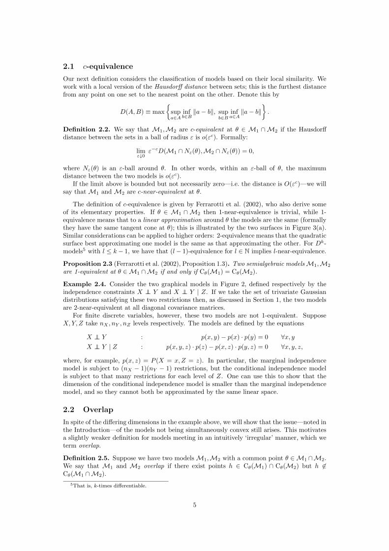
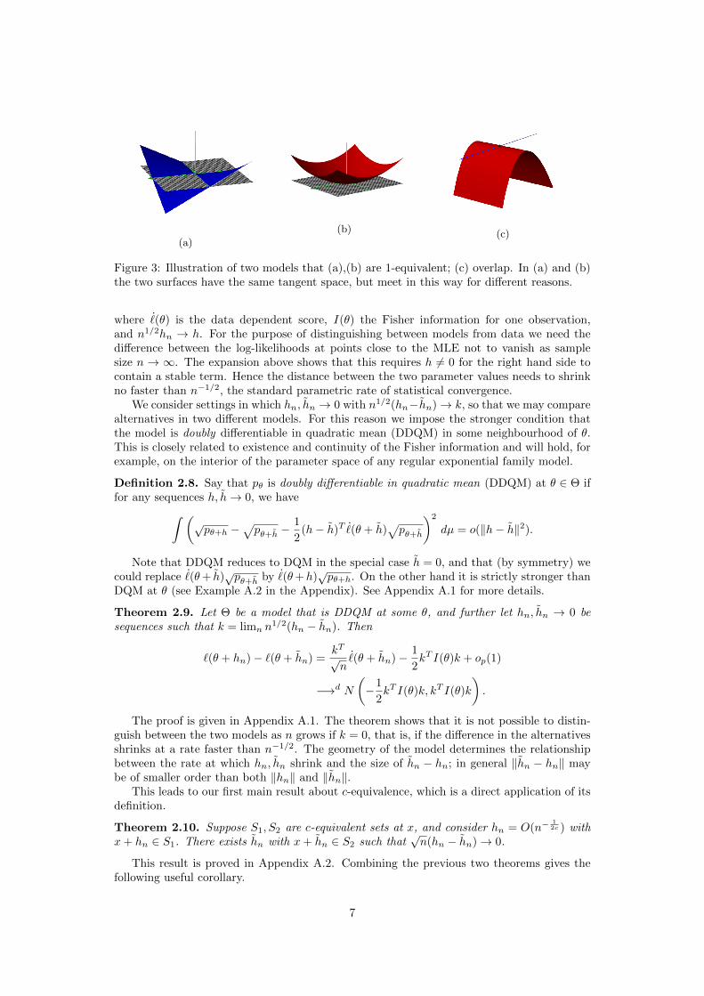
The definition of c-equivalence is given by Ferrarotti et al. (2002), who also derive someof its elementary properties. If θ ∈ M1 ∩ M2 then 1-near-equivalence is trivial, while 1-equivalence means that to a linear approximation around θ the models are the same (formallythey have the same tangent cone at θ); this is illustrated by the two surfaces in Figure 3(a).Similar considerations can be applied to higher orders: 2-equivalence means that the quadraticsurface best approximating one model is the same as that approximating the other. For Dk-models5 with l ≤ k− 1, we have that (l− 1)-equivalence for l ∈ N implies l-near-equivalence.

Proposition 2.3 (Ferrarotti et al. (2002), Proposition 1.3). Two semialgebraic modelsM1,M2

are 1-equivalent at θ ∈M1 ∩M2 if and only if Cθ(M1) = Cθ(M2).

Example 2.4. Consider the two graphical models in Figure 2, defined respectively by theindependence constraints X ⊥⊥ Y and X ⊥⊥ Y | Z. If we take the set of trivariate Gaussiandistributions satisfying these two restrictions then, as discussed in Section 1, the two modelsare 2-near-equivalent at all diagonal covariance matrices.

For finite discrete variables, however, these two models are not 1-equivalent. SupposeX,Y, Z take nX , nY , nZ levels respectively. The models are defined by the equations

X ⊥⊥ Y : p(x, y)− p(x) · p(y) = 0 ∀x, yX ⊥⊥ Y | Z : p(x, y, z) · p(z)− p(x, z) · p(y, z) = 0 ∀x, y, z,

where, for example, p(x, z) = P (X = x, Z = z). In particular, the marginal independencemodel is subject to (nX − 1)(nY − 1) restrictions, but the conditional independence modelis subject to that many restrictions for each level of Z. One can use this to show that thedimension of the conditional independence model is smaller than the marginal independencemodel, and so they cannot both be approximated by the same linear space.

2.2 Overlap

In spite of the differing dimensions in the example above, we will show that the issue—noted inthe Introduction—of the models not being simultaneously convex still arises. This motivatesa slightly weaker definition for models meeting in an intuitively ‘irregular’ manner, which weterm overlap.

Definition 2.5. Suppose we have two modelsM1,M2 with a common point θ ∈M1 ∩M2.We say that M1 and M2 overlap if there exist points h ∈ Cθ(M1) ∩ Cθ(M2) but h 6∈Cθ(M1 ∩M2).

5That is, k-times differentiable.

5

In other words, there are tangent vectors that can be obtained in either model, but not intheir intersection. Note that necessarily we have Cθ(M1 ∩M2) ⊆ Cθ(M1)∩Cθ(M2), so thedefinition asks that this is a strict inclusion. For distinct, regular algebraic models, overlapis implied by 1-equivalence.

Lemma 2.6. Let M1 and M2 be algebraic models that are 1-equivalent and regular at θ, butnot equal in a neighbourhood of θ. Then M1 and M2 overlap at θ.

Proof. Suppose that, at θ, the models do not overlap and are 1-equivalent. We will show thatthey are equal in a neighbourhood of θ.

SinceM1 is regular at θ we can assume that it is an irreducible model, else replace it withits unique irreducible component containing θ (similarly for M2). The condition that themodels are 1-equivalent implies Cθ(M1) = Cθ(M2), and no overlap means Cθ(M1 ∩M2) =Cθ(M1) ∩ Cθ(M2) = Cθ(M1).

On the other hand, M1 ∩M2 is an algebraic submodel of M1, so it is either equal toM1 or has strictly lower dimension. If the latter, then Cθ(M1 ∩M2) would be of this samelower dimension (Cox et al., 2008, Theorem 9.7.8), and hence is a strict subset. Since we havealready seen that M1 ∩M2 has the same tangent cone as M1, it must be that the formerpossibility holds; that is,M1 ∩M2 =M1, in a neighbourhood of θ. Clearly the same is truefor M2, which proves the result.

The same result could be applied to analytic models, defined by the zeroes of analyticfunctions, since these functions are (by definition) arbitrarily well approximated by theirTaylor series.

Remark 2.7. Without assuming that models are analytic, one can construct examples thatare ‘regular’ in most of the usual statistical senses, but for which the previous result fails.As an example of how things can go wrong, consider the function f(x) = e−1/x2

sin(1/x2)(taking f(0) = 0); this is a C∞ function, but is not analytic at x = 0 (all its derivatives beingzero at this point).

Now let M1 = (x, 0) : x ∈ R and M2 = (x, f(x)) : x ∈ R. These models are c-equivalent for every c ∈ N, but are not equal. However, in contrast to the result of Lemma2.6 they do not overlap. Both sets have tangent cone equal toM1, and since f has infinitelymany roots in any neighbourhood of 0, the tangent cone of M1 ∩M2 is also M1.

A canonical example of sets that overlap but are not 1-equivalent is given by the subsetsof R3 shown in Figure 3(c); M1 = (x, y, z) : y = z = 0 (in blue) and M2 = (x, y, z) :z = −x2 (in red) have M1 ∩M2 = 0. The tangent cone of M2 is the plane z = 0, whileM1 is its own tangent cone and therefore C0(M1) ⊆ C0(M2) and C0(M1)∩C0(M2) =M1.However, C0(M1∩M2) = 0, so the inclusion is strict. In words, we can approach the originalong a line that becomes tangent to the x-axis in either model, but not in the intersection.The blue model has smaller dimension than the red so they clearly not 1-equivalent.

Typically it is hard to show that two models are not 1-equivalent (or do not overlap)anywhere in the parameter space: indeed the difficulty of verifying such global conditionsis one of our motivations for considering these local criteria instead. However, for algebraicmodels we can often show that such points are at most a set of zero measure within a largeclass of ‘interesting’ submodels. To be more precise, if two models are not 1-equivalent atsome model of total independence (say θ0), then they are also 1-equivalent almost nowherewithin any algebraic model that contains θ0.

2.3 Statistical Power

We will assume that all the models we consider satisfy standard parametric regularity con-ditions, in particular differentiability in quadratic mean (DQM), which yields the familiarasymptotic expansion of the log-likelihood `(θ) (see, e.g. van der Vaart, 1998):

`(θ + hn)− `(θ) =hT√n

˙(θ)− 1

2hT I(θ)h+ op(1), (1)

6

(a)

(b) (c)

Figure 3: Illustration of two models that (a),(b) are 1-equivalent; (c) overlap. In (a) and (b)the two surfaces have the same tangent space, but meet in this way for different reasons.

where ˙(θ) is the data dependent score, I(θ) the Fisher information for one observation,and n1/2hn → h. For the purpose of distinguishing between models from data we need thedifference between the log-likelihoods at points close to the MLE not to vanish as samplesize n → ∞. The expansion above shows that this requires h 6= 0 for the right hand side tocontain a stable term. Hence the distance between the two parameter values needs to shrinkno faster than n−1/2, the standard parametric rate of statistical convergence.

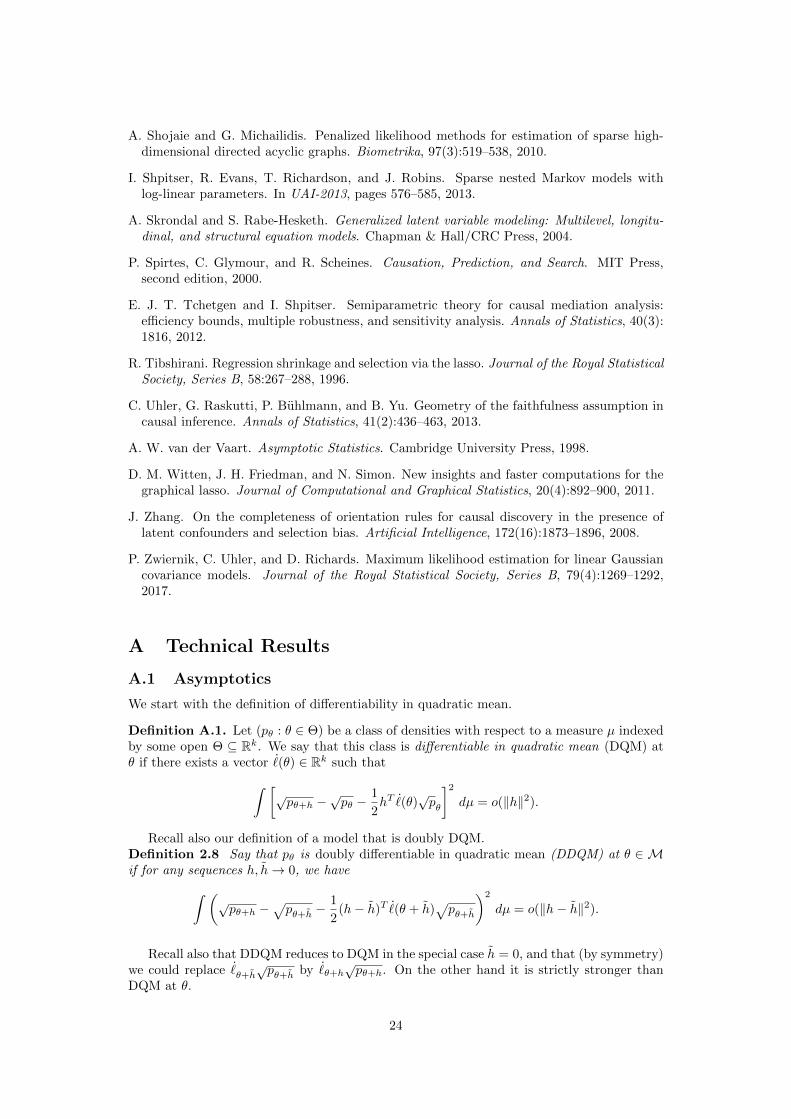
We consider settings in which hn, hn → 0 with n1/2(hn−hn)→ k, so that we may comparealternatives in two different models. For this reason we impose the stronger condition thatthe model is doubly differentiable in quadratic mean (DDQM) in some neighbourhood of θ.This is closely related to existence and continuity of the Fisher information and will hold, forexample, on the interior of the parameter space of any regular exponential family model.

Definition 2.8. Say that pθ is doubly differentiable in quadratic mean (DDQM) at θ ∈ Θ iffor any sequences h, h→ 0, we have∫ (

√pθ+h −

√pθ+h −

1

2(h− h)T ˙(θ + h)

√pθ+h

)2

dµ = o(‖h− h‖2).

Note that DDQM reduces to DQM in the special case h = 0, and that (by symmetry) wecould replace ˙(θ+ h)

√pθ+h by ˙(θ+h)

√pθ+h. On the other hand it is strictly stronger than

DQM at θ (see Example A.2 in the Appendix). See Appendix A.1 for more details.

Theorem 2.9. Let Θ be a model that is DDQM at some θ, and further let hn, hn → 0 besequences such that k = limn n

1/2(hn − hn). Then

`(θ + hn)− `(θ + hn) =kT√n

˙(θ + hn)− 1

2kT I(θ)k + op(1)

−→d N

(−1

2kT I(θ)k, kT I(θ)k

).

The proof is given in Appendix A.1. The theorem shows that it is not possible to distin-guish between the two models as n grows if k = 0, that is, if the difference in the alternativesshrinks at a rate faster than n−1/2. The geometry of the model determines the relationshipbetween the rate at which hn, hn shrink and the size of hn − hn; in general ‖hn − hn‖ maybe of smaller order than both ‖hn‖ and ‖hn‖.

This leads to our first main result about c-equivalence, which is a direct application of itsdefinition.

Theorem 2.10. Suppose S1, S2 are c-equivalent sets at x, and consider hn = O(n−12c ) with

x+ hn ∈ S1. There exists hn with x+ hn ∈ S2 such that√n(hn − hn)→ 0.

This result is proved in Appendix A.2. Combining the previous two theorems gives thefollowing useful corollary.

7

Corollary 2.11. Let Θ be a model that is DDQM at some θ, and M1,M2 ⊂ Θ be sub-models. If M1,M2 are c-equivalent (respectively c-near-equivalent) at θ then they cannot

be asymptotically distinguished under local alternatives to θ of order O(n−12c ) (respectively

o(n−12c )).

All models that intersect are 1-near-equivalent, and therefore we recover the usual para-metric rate: we have power only if hn shrinks at n−1/2 or slower. For 1-equivalent modelsthis is not enough: a rate of n−1/2 will be too fast for us to tell whether our parameters arein M1 or M2. In practice, regular models that are 1-equivalent are also 2-near-equivalent,so any rate quicker than n−1/4 is also too fast.

2.4 Convexity

A second consequence of having 1-equivalent regular models is that it is not possible to have aparameterization with respect to which both models are convex; in fact, this is true even underthe weaker assumption of overlap. Some automatic model selection methods such as the lasso(Tibshirani, 1996) rely on a convex parameterization, usually constructed by ensuring thatinteresting submodels correspond to coordinate zeroes (e.g. θ1 = 0). Such selection methodscannot be directly applied to model classes that contain overlapping models.

Theorem 2.12. Suppose M1 and M2 are distinct models that overlap at a point θ on theirrelative interiors. Then there is no parameterization with respect to which both these modelsare convex in a neighbourhood of θ.

Proof. This is just a statement about sets under differentiable maps with differentiable in-verses; note that tangent cones and spaces are isomorphically preserved under such transfor-mations. We will prove the contrapositive: if two sets C,D with x ∈ C ∩D are convex (in aneighbourhood of x) then they do not overlap at x.

The affine hull of any convex set C is the unique minimal affine space A containing C.Furthermore, by definition of the relative interior, for every x ∈ C int there is a neighbourhoodof x in which C and A are identical, i.e. C coincides with the affine space A at x.

Now, suppose two sets C and D are both convex and x ∈ C int ∩Dint. Then they coincidewith affine spaces say A,B and hence are their own tangent spaces at x. This implies thatC ∩ D coincides with the affine space A ∩ B, and hence the tangent cone of C ∩ D is justA∩B. Hence C and D do not overlap. Since isomorphic maps cannot alter the tangent conesof these sets, this is true regardless of the parameterization chosen.

Intuitively, one can reparameterize a regular model such that (at least locally to some pointθ) the model is convex. However, this cannot be done simultaneously for two overlappingmodels. This is illustrated in Figure 4. The result fails if θ is not required to be a point onthe relative interior, a counterexample being modelsM1 = θ2 ≥ θ2

1 andM2 = θ2 ≤ −θ21

with θ = (0, 0).

Remark 2.13. Many convex methods, including the lasso, proceed by optimizing a convexfunction over a parameter space containing all submodels of interest. In the case of the lasso,this function has ‘cusps’ on submodels of interest that lead to a non-zero probability that theoptimum lies exactly on the model. Theorem 2.12 shows that such a procedure cannot beconvex if the class contains overlapping models, since the submodels themselves cannot bemade convex. Any submodel that is not convex cannot represent a cusp in a convex function,and therefore we cannot obtain a non-zero probability of selecting such a model.

The nature of this impossibility result should perhaps not be surprising, since all versionsof the lasso in the context of ordinary linear models place a restriction on the collinearity of thedifferent parameters in the form of restricted isometry properties or similar (for an overviewsee, for example, Buhlmann and van de Geer, 2011). In the case of 1-equivalent models, aswe move closer to the point of intersection the angle between the two models shrinks to zero,so no such property could possibly hold. For models that overlap the problem is similar, but

8

⇒(a)

⇒(b)

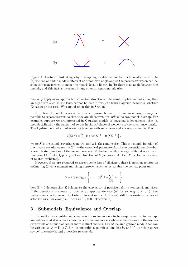
Figure 4: Cartoon illustrating why overlapping models cannot be made locally convex. In(a) the red and blue models intersect at a non-zero angle and so the parameterization can besmoothly transformed to make the models locally linear. In (b) there is no angle between themodels, and this fact is invariant in any smooth reparameterization.

may only apply as we approach from certain directions. The result implies, in particular, thatan algorithm such as the lasso cannot be used directly to learn Bayesian networks, whetherGaussian or discrete. We expand upon this in Section 4.

If a class of models is non-convex when parameterized in a canonical way, it may bepossible to reparameterize so that they are all convex, but only if no two models overlap. Forexample, suppose we are interested in Gaussian models of marginal independence; that is,models defined by the pattern of zeroes in the off-diagonal elements of the covariance matrix.The log-likelihood of a multivariate Gaussian with zero mean and covariance matrix Σ is

`(Σ;S) =n

2

log det Σ−1 − tr(SΣ−1)

,

where S is the sample covariance matrix and n is the sample size. This is a simple function ofthe inverse covariance matrix Σ−1—the canonical parameter for this exponential family—buta complicated function of the mean parameter Σ. Indeed, while the log-likelihood is a convexfunction of Σ−1, it is typically not as a function of Σ (see Zwiernik et al., 2017, for an overviewof related problems).

However, if we are prepared to accept some loss of efficiency, there is nothing to stop usestimating Σ via a moment matching approach, such as by solving the convex program:

Σ = arg minΣ0

‖Σ− S‖2 + ν∑i<j

|σij |

;

here Σ 0 denotes that Σ belongs to the convex set of positive definite symmetric matrices.If the penalty ν is chosen to grow at an appropriate rate (nδ for some 1

2 < δ < 1) thenunder some conditions on the Fisher information for Σ, this will still be consistent for modelselection (see, for example, Rocha et al., 2009, Theorem 5).

3 Submodels, Equivalence and Overlap

In this section we consider sufficient conditions for models to be c-equivalent or to overlap.We will see that it is often a consequence of having models whose intersections are themselvesexpressible as a union of two or more distinct models. LetM be an algebraic model that canbe written as M = V1 ∪ V2 for incomparable algebraic submodels V1 and V2; in this case wesay M is reducible, and otherwise irreducible.

9

3.1 Identifying c-equivalence

For the example in Figure 2, the 1-equivalence of the two models M1 = Π : X ⊥⊥ Y andM2 = Π : X ⊥⊥ Y | Z was closely related to the fact that if either X ⊥⊥ Z or Y ⊥⊥ Z holds,thenM1 andM2 intersect. This means that their intersection is a reducible model, as it canbe non-trivially expressed as the union of two or more models. It follows that at any pointswhere both the submodelsMX⊥⊥Z andMY⊥⊥Z hold, the two original models are 1-equivalent.This is because any direction inM1 (orM2) away from the point of intersectionM1∩M2 canbe written as a linear combination of (limits of) vectors that lie in one ofMX⊥⊥Z orMY⊥⊥Z ;the partial derivatives of the distance between M1 and M2 in these directions are zero, andso any directional derivative of this quantity is also zero. This is illustrated in Figure 3(a),which shows two surfaces intersecting along two lines: in directions that are diagonal to theselines, the two surfaces separate at a rate that is at most quadratic.

It is not necessary for models to intersect in this manner in order to be 1-equivalent: forexample, the surfaces z = 0 and z = x2 + y2 intersect only at the point (0, 0, 0) (see Figure3(b)). However, many models that are 1-equivalent do intersect along at least two submodels,including most of the substantive examples that we are aware of; the time series models inSection 5.2 are an exception. If c > 2 submodels are involved in the intersection, then we willsee that the original models are c-near-equivalent and asymptotic rates for local alternativeswill be even slower than n−1/4.

To formalize this, we use the next result. Define the normal space of a D1 surface M tobe the orthogonal complement of its tangent space, Tθ(M)⊥.

Theorem 3.1. Suppose M1,M2 and N1, . . . ,Nm are Dm manifolds all containing a pointθ, and such that Ni ∩M1 = Ni ∩M2 for i = 1, . . . ,m. Suppose also that Tθ(Ni ∩Mj) =Tθ(Ni) ∩ Tθ(Mj) for each i = 1, . . . ,m and j = 1, 2, and further that the normal vectorspaces Tθ(N1)⊥, . . . ,Tθ(Nm)⊥ all have linearly independent bases. Then M1 and M2 arem-near-equivalent at θ.

Note that an algebraic set is always a Dm manifold within a ball around a regular point. Inwords, there are m distinct submodels on whichM1 andM2 intersect; in order to distinguishbetweenM1 andM2, we need to ‘move away’ from all the submodelsNi. Linear independenceof the normal spaces ensures that we cannot move directly away from several submodels atonce.

Proof. See the Appendix section A.3.

Perhaps an easier way to think about the normal vector spaces is in terms of the submodelsbeing defined by ‘independent constraints’; in particular, by constraints defined on differentparts of the model. If N1 is defined by the set of points that are zeros of the functionsf1, . . . , fk, then Tθ(N1)⊥ contains the space spanned by the Jacobian J(f1, . . . , fk). If N2 issimilarly defined by g1, . . . , gl then the condition is equivalent to saying that the Jacobian ofall k + l functions has full rank k + l at θ.

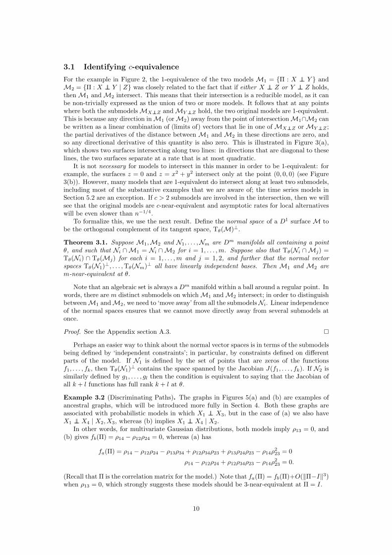
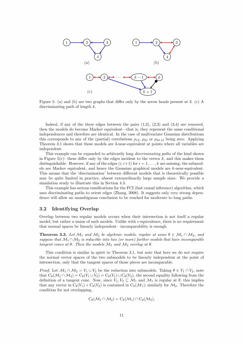
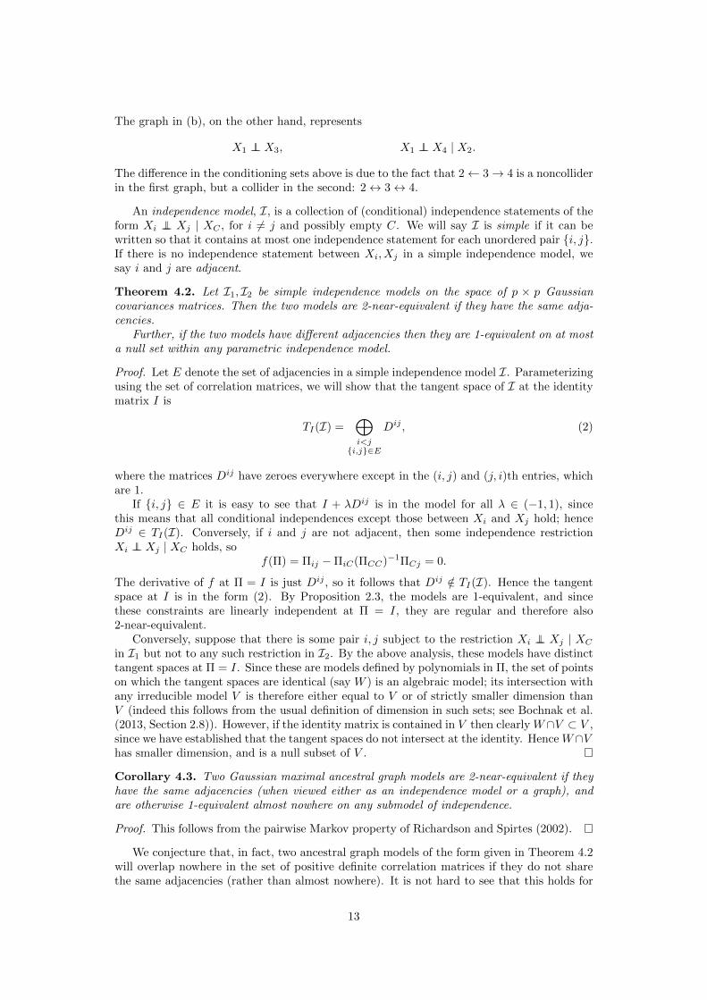
Example 3.2 (Discriminating Paths). The graphs in Figures 5(a) and (b) are examples ofancestral graphs, which will be introduced more fully in Section 4. Both these graphs areassociated with probabilistic models in which X1 ⊥⊥ X3, but in the case of (a) we also haveX1 ⊥⊥ X4 | X2, X3, whereas (b) implies X1 ⊥⊥ X4 | X2.

In other words, for multivariate Gaussian distributions, both models imply ρ13 = 0, and(b) gives fb(Π) = ρ14 − ρ12ρ24 = 0, whereas (a) has

fa(Π) = ρ14 − ρ12ρ24 − ρ13ρ34 + ρ12ρ34ρ23 + ρ13ρ24ρ23 − ρ14ρ223 = 0

ρ14 − ρ12ρ24 + ρ12ρ34ρ23 − ρ14ρ223 = 0.

(Recall that Π is the correlation matrix for the model.) Note that fa(Π) = fb(Π)+O(‖Π−I‖3)when ρ13 = 0, which strongly suggests these models should be 3-near-equivalent at Π = I.

10

1 2 3

4

(a)

1 2 3

4

(b)

1 2 . . . k − 1 k

k + 1(c)

Figure 5: (a) and (b) are two graphs that differ only by the arrow heads present at 3. (c) Adiscriminating path of length k.

Indeed, if any of the three edges between the pairs (1,2), (2,3) and (3,4) are removed,then the models do become Markov equivalent—that is, they represent the same conditionalindependences and therefore are identical. In the case of multivariate Gaussian distributionsthis corresponds to any of the (partial) correlations ρ12, ρ23 or ρ34·12 being zero. ApplyingTheorem 3.1 shows that these models are 3-near-equivalent at points where all variables areindependent.

This example can be expanded to arbitrarily long discriminating paths of the kind shownin Figure 5(c): these differ only by the edges incident to the vertex k, and this makes themdistinguishable. However, if any of the edges (i, i+1) for i = 1, . . . , k are missing, the submod-els are Markov equivalent, and hence the Gaussian graphical models are k-near-equivalent.This means that the ‘discrimination’ between different models that is theoretically possiblemay be quite limited in practice, absent extraordinarily large sample sizes. We provide asimulation study to illustrate this in Section 4.3.

This example has serious ramifications for the FCI (fast causal inference) algorithm, whichuses discriminating paths to orient edges (Zhang, 2008). It suggests only very strong depen-dence will allow an unambiguous conclusion to be reached for moderate to long paths.

3.2 Identifying Overlap

Overlap between two regular models occurs when their intersection is not itself a regularmodel, but rather a union of such models. Unlike with c-equivalence, there is no requirementthat normal spaces be linearly independent—incomparability is enough.

Theorem 3.3. Let M1 and M2 be algebraic models, regular at some θ ∈ M1 ∩M2, andsuppose that M1 ∩M2 is reducible into two (or more) further models that have incomparabletangent cones at θ. Then the models M1 and M2 overlap at θ.

This condition is similar in spirit to Theorem 3.1, but note that here we do not requirethe normal vector spaces of the two submodels to be linearly independent at the point ofintersection, only that the tangent spaces of those pieces are incomparable.

Proof. Let M1 ∩M2 = V1 ∪ V2 be the reduction into submodels. Taking θ ∈ V1 ∩ V2, notethat Cθ(M1 ∩M2) = Cθ(V1 ∪ V2) = Cθ(V1)∪Cθ(V2), the second equality following from thedefinition of a tangent cone. Now, since V1, V2 ⊆ M1 and M1 is regular at θ, this impliesthat any vector in Cθ(V1) + Cθ(V2) is contained in Cθ(M1); similarly for M2. Therefore thecondition for not overlapping,

Cθ(M1 ∩M2) = Cθ(M1) ∩ Cθ(M2),

11

holds only if Cθ(V1) + Cθ(V2) ⊆ Cθ(V1)∪Cθ(V2). This occurs only if one of Cθ(V1) or Cθ(V2)is a subspace of the other, but this was ruled out by hypothesis.

Example 3.4. As already noted in Examples 1.2 and 2.4, the Gaussian graphical modelsdefined respectively by the independences M1 : X ⊥⊥ Y and M2 : X ⊥⊥ Y | Z are 1-equivalent at diagonal covariance matrices, but the corresponding discrete models are not.This is because—taking X,Y, Z to be binary—the three-way interaction parameter

λXY Z ≡1

8

∑x,y,z∈0,1

(−1)|x+y+z| logP (X = x, Y = y, Z = z)

is zero in the conditional independence model6, but essentially unrestricted in the marginalindependence model. However, the intersection of M1 and M2 for binary X,Y, Z is the setof distributions such that either X ⊥⊥ Y,Z or Y ⊥⊥ X,Z, and these correspond respectivelyto the submodels

λXY = λXZ = λXY Z = 0 or λXY = λY Z = λXY Z = 0,

also defined by zeros of polynomials in P (see Appendix B for full definitions). These mod-els satisfy the conditions of Theorem 3.3 at points of total independence ⊥⊥X,Y, Z, andtherefore M1 and M2 do overlap.

4 Directed and Ancestral Graph Models

In this section we focus on two classes of graphical models: Bayesian network models, andthe more general ancestral graph models. A more detailed explanation of the relevant theorycan be found in Spirtes et al. (2000) and Richardson and Spirtes (2002).

4.1 Ancestral Graphs

A maximal ancestral graph (MAG) is a simple, mixed graph with three kinds of edge, undi-rected (−), directed (→) and bidirected (↔). Special cases of ancestral graphs include di-rected acyclic graphs, undirected graphs and bidirected graphs, but not chain graphs. Thereare some technical restrictions on the structure of the graph which we omit here for brevity:the key detail is that—under the usual Markov property—the model implies a conditionalindependence constraint between each pair of vertices if (and only if) they are not joinedby any sort of edge in the graph (Richardson and Spirtes, 2002). The set that needs to beconditioned upon to obtain the independence depends on the presence of colliders in thegraph. A collider is a pair of edges that meet with two arrowheads at a vertex k: for example,i→ k ← j or i→ k ↔ j. Any other configuration is called a noncollider. We say the collideror noncollider is unshielded if i and j are not joined by an edge.

The special case of an ancestral graph model in which all edges are directed yields aBayesian network (BN) model, widely used in causal inference and in machine learning(Bishop, 2007; Pearl, 2009). The additional undirected and bidirected edges allow MAGsto represent the set of conditional independence models generated by marginalizing and con-ditioning a BN model. Ancestral graphs are therefore useful in causal modelling, since theyrepresent the conditional independence model implied by a causal structure with hidden andselection variables.

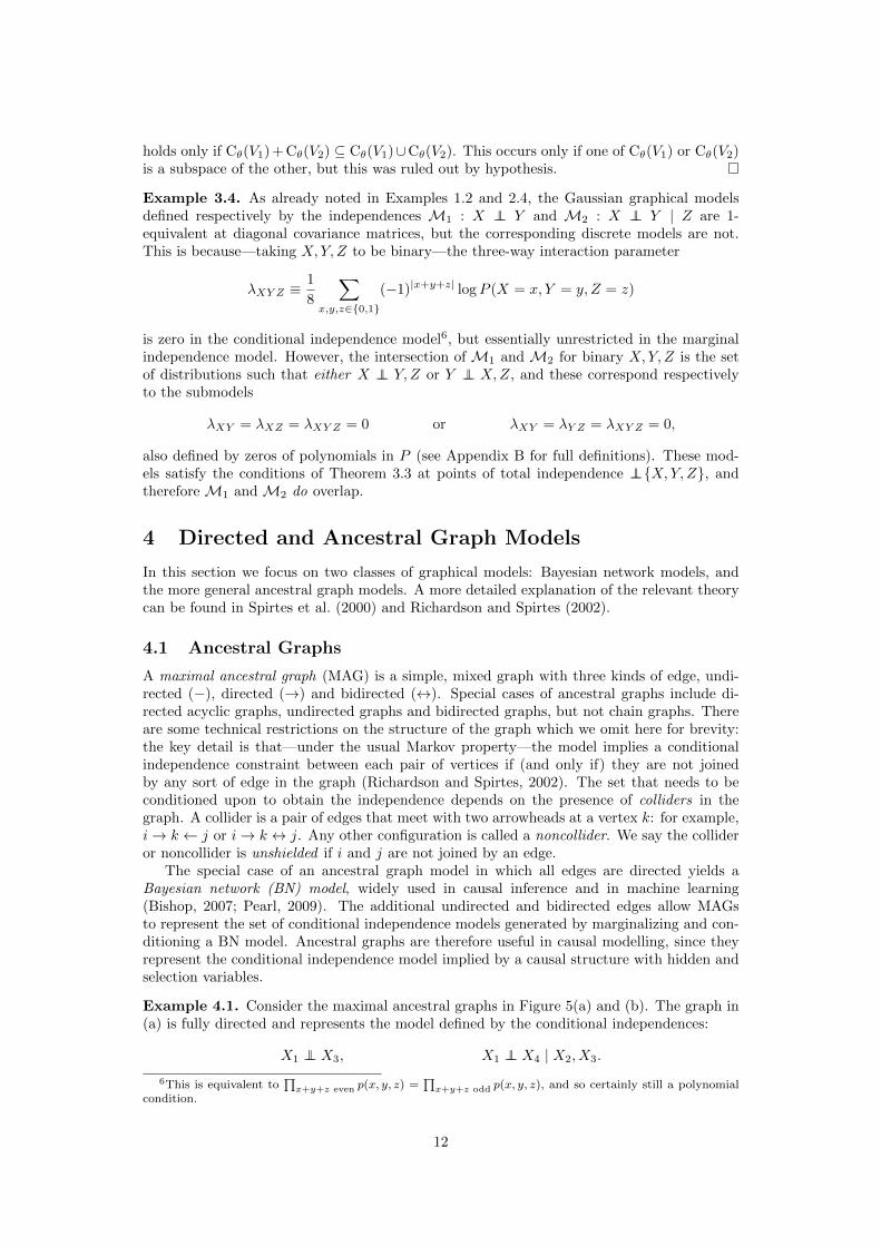
Example 4.1. Consider the maximal ancestral graphs in Figure 5(a) and (b). The graph in(a) is fully directed and represents the model defined by the conditional independences:

X1 ⊥⊥ X3, X1 ⊥⊥ X4 | X2, X3.

6This is equivalent to∏

x+y+z even p(x, y, z) =∏

x+y+z odd p(x, y, z), and so certainly still a polynomialcondition.

12

The graph in (b), on the other hand, represents

X1 ⊥⊥ X3, X1 ⊥⊥ X4 | X2.

The difference in the conditioning sets above is due to the fact that 2← 3→ 4 is a noncolliderin the first graph, but a collider in the second: 2↔ 3↔ 4.

An independence model, I, is a collection of (conditional) independence statements of theform Xi ⊥⊥ Xj | XC , for i 6= j and possibly empty C. We will say I is simple if it can bewritten so that it contains at most one independence statement for each unordered pair i, j.If there is no independence statement between Xi, Xj in a simple independence model, wesay i and j are adjacent.

Theorem 4.2. Let I1, I2 be simple independence models on the space of p × p Gaussiancovariances matrices. Then the two models are 2-near-equivalent if they have the same adja-cencies.

Further, if the two models have different adjacencies then they are 1-equivalent on at mosta null set within any parametric independence model.

Proof. Let E denote the set of adjacencies in a simple independence model I. Parameterizingusing the set of correlation matrices, we will show that the tangent space of I at the identitymatrix I is

TI(I) =⊕i<j

i,j∈E

Dij , (2)

where the matrices Dij have zeroes everywhere except in the (i, j) and (j, i)th entries, whichare 1.

If i, j ∈ E it is easy to see that I + λDij is in the model for all λ ∈ (−1, 1), sincethis means that all conditional independences except those between Xi and Xj hold; henceDij ∈ TI(I). Conversely, if i and j are not adjacent, then some independence restrictionXi ⊥⊥ Xj | XC holds, so

f(Π) = Πij −ΠiC(ΠCC)−1ΠCj = 0.

The derivative of f at Π = I is just Dij , so it follows that Dij /∈ TI(I). Hence the tangentspace at I is in the form (2). By Proposition 2.3, the models are 1-equivalent, and sincethese constraints are linearly independent at Π = I, they are regular and therefore also2-near-equivalent.

Conversely, suppose that there is some pair i, j subject to the restriction Xi ⊥⊥ Xj | XC

in I1 but not to any such restriction in I2. By the above analysis, these models have distincttangent spaces at Π = I. Since these are models defined by polynomials in Π, the set of pointson which the tangent spaces are identical (say W ) is an algebraic model; its intersection withany irreducible model V is therefore either equal to V or of strictly smaller dimension thanV (indeed this follows from the usual definition of dimension in such sets; see Bochnak et al.(2013, Section 2.8)). However, if the identity matrix is contained in V then clearly W∩V ⊂ V ,since we have established that the tangent spaces do not intersect at the identity. Hence W∩Vhas smaller dimension, and is a null subset of V .

Corollary 4.3. Two Gaussian maximal ancestral graph models are 2-near-equivalent if theyhave the same adjacencies (when viewed either as an independence model or a graph), andare otherwise 1-equivalent almost nowhere on any submodel of independence.

Proof. This follows from the pairwise Markov property of Richardson and Spirtes (2002).

We conjecture that, in fact, two ancestral graph models of the form given in Theorem 4.2will overlap nowhere in the set of positive definite correlation matrices if they do not sharethe same adjacencies (rather than almost nowhere). It is not hard to see that this holds for

13

models of different dimension, since these models are regular and therefore will share thisdimension everywhere. To prove it in general seems challenging; the result above is sufficientfor most practical purposes.

Corollary 4.4. Let G,H be chain graphs with the same adjacencies under any of the in-terpretations given in Drton (2009b) (not necessarily the same interpretation). Then thecorresponding models are 2-near-equivalent.

Note that Remark 5 of Drton (2009b) makes clear that pairwise independences are suffi-cient to define Gaussian chain graph models.

4.2 Discrete Data

The picture is slightly rosier if we consider discrete data instead. A well known result ofChickering (1996) shows that finding an optimal Bayesian Network for discrete data is anNP-hard problem; in other words, it is computationally difficult. However, we find that froma statistical point of view, it is somewhat easier than in the Gaussian case.

Theorem 4.5. No two distinct, binary, maximal ancestral graph models are 1-equivalent atthe model of total independence.

Proof. See the Appendix, Section C.

Although distinct, discrete MAG models (and therefore BN models) are never 1-equivalent,they do still overlap, as our next result demonstrates.

Proposition 4.6. Let M(G1),M(G2) be two discrete Bayesian network models such thati→ k ← j is an unshielded collider in G1 but an unshielded noncollider in G2. Then, if Xk isbinary, the two models overlap.

Proof. See the Appendix, Section C.

Remark 4.7. The condition that some variables are binary is, in fact, unnecessary—seeRemark C.2 for more details on the general finite discrete case.

Bayesian network models that are consistent with a single topological ordering of thevertices do not overlap, because their intersection is always another BN model. We cantherefore work with a class defined by the subgraphs of a single complete BN in order toavoid the problems associated with overlap.

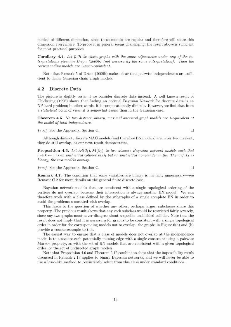
This leads to the question of whether any other, perhaps larger, subclasses share thisproperty. The previous result shows that any such subclass would be restricted fairly severely,since any two graphs must never disagree about a specific unshielded collider. Note that theresult does not imply that it is necessary for graphs to be consistent with a single topologicalorder in order for the corresponding models not to overlap; the graphs in Figure 6(a) and (b)provide a counterexample to this.

The easiest way to ensure that a class of models does not overlap at the independencemodel is to associate each potentially missing edge with a single constraint using a pairwiseMarkov property, as with the set of BN models that are consistent with a given topologicalorder, or the set of undirected graph models.

Note that Proposition 4.6 and Theorem 2.12 combine to show that the impossibility resultdiscussed in Remark 2.13 applies to binary Bayesian networks, and we will never be able touse a lasso-like method to consistently select from this class under standard conditions.

14

X Y

Z W

(a)

X Y

Z W

(b)

X

Z

Y

(c)

Figure 6: (a) and (b) two Bayesian networks which do not overlap but are not consistent witha single topological order. (c) A simple causal model.

4.3 Discriminating Paths

Example 3.2 introduced the notion of a discriminating path, which allows the identificationof colliders in an ancestral graph. Formally, define the ancestral graphs Gk and G′k as havingvertices 1, . . . , k+1, with a path 1↔ 2↔ · · · ↔ k and directed edges from each of 2, . . . , k−1to k + 1. In addition, Gk has the edges k ↔ k + 1, while G′k has k → k + 1; the graphs areshown in Figure 5(c), with only the final edge left ambiguous. The path from 1 to k + 1 isknown as a discriminating path, and its structure allows us to determine whether there is acollider at k (as in Gk) or not (as in G′k).

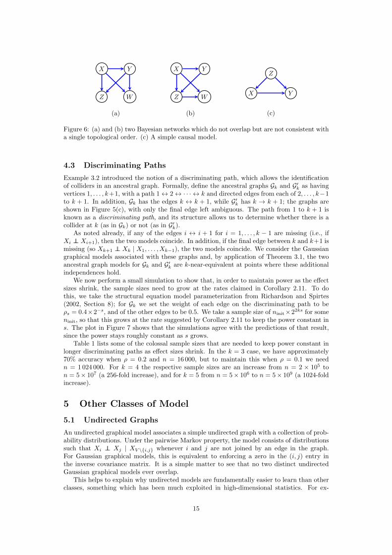
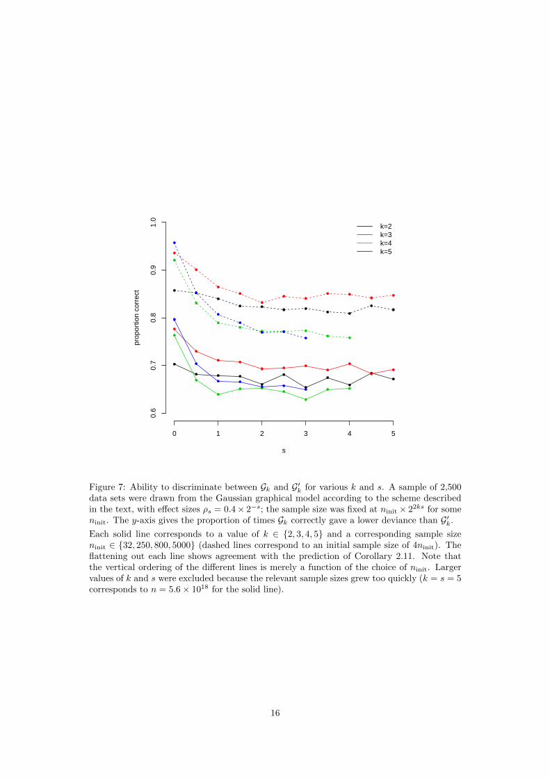
As noted already, if any of the edges i ↔ i + 1 for i = 1, . . . , k − 1 are missing (i.e., ifXi ⊥⊥ Xi+1), then the two models coincide. In addition, if the final edge between k and k+1 ismissing (so Xk+1 ⊥⊥ Xk | X1, . . . , Xk−1), the two models coincide. We consider the Gaussiangraphical models associated with these graphs and, by application of Theorem 3.1, the twoancestral graph models for Gk and G′k are k-near-equivalent at points where these additionalindependences hold.

We now perform a small simulation to show that, in order to maintain power as the effectsizes shrink, the sample sizes need to grow at the rates claimed in Corollary 2.11. To dothis, we take the structural equation model parameterization from Richardson and Spirtes(2002, Section 8); for Gk we set the weight of each edge on the discriminating path to beρs = 0.4×2−s, and of the other edges to be 0.5. We take a sample size of ninit×22ks for someninit, so that this grows at the rate suggested by Corollary 2.11 to keep the power constant ins. The plot in Figure 7 shows that the simulations agree with the predictions of that result,since the power stays roughly constant as s grows.

Table 1 lists some of the colossal sample sizes that are needed to keep power constant inlonger discriminating paths as effect sizes shrink. In the k = 3 case, we have approximately70% accuracy when ρ = 0.2 and n = 16 000, but to maintain this when ρ = 0.1 we needn = 1 024 000. For k = 4 the respective sample sizes are an increase from n = 2 × 105 ton = 5× 107 (a 256-fold increase), and for k = 5 from n = 5× 106 to n = 5× 109 (a 1024-foldincrease).

5 Other Classes of Model

5.1 Undirected Graphs

An undirected graphical model associates a simple undirected graph with a collection of prob-ability distributions. Under the pairwise Markov property, the model consists of distributionssuch that Xi ⊥⊥ Xj | XV \i,j whenever i and j are not joined by an edge in the graph.For Gaussian graphical models, this is equivalent to enforcing a zero in the (i, j) entry inthe inverse covariance matrix. It is a simple matter to see that no two distinct undirectedGaussian graphical models ever overlap.

This helps to explain why undirected models are fundamentally easier to learn than otherclasses, something which has been much exploited in high-dimensional statistics. For ex-

15

0 1 2 3 4 5

0.6

0.7

0.8

0.9

1.0

k=2k=3k=4k=5

s

prop

ortio

n co

rrec

t

Figure 7: Ability to discriminate between Gk and G′k for various k and s. A sample of 2,500data sets were drawn from the Gaussian graphical model according to the scheme describedin the text, with effect sizes ρs = 0.4× 2−s; the sample size was fixed at ninit × 22ks for someninit. The y-axis gives the proportion of times Gk correctly gave a lower deviance than G′k.

Each solid line corresponds to a value of k ∈ 2, 3, 4, 5 and a corresponding sample sizeninit ∈ 32, 250, 800, 5000 (dashed lines correspond to an initial sample size of 4ninit). Theflattening out each line shows agreement with the prediction of Corollary 2.11. Note thatthe vertical ordering of the different lines is merely a function of the choice of ninit. Largervalues of k and s were excluded because the relevant sample sizes grew too quickly (k = s = 5corresponds to n = 5.6× 1018 for the solid line).

16

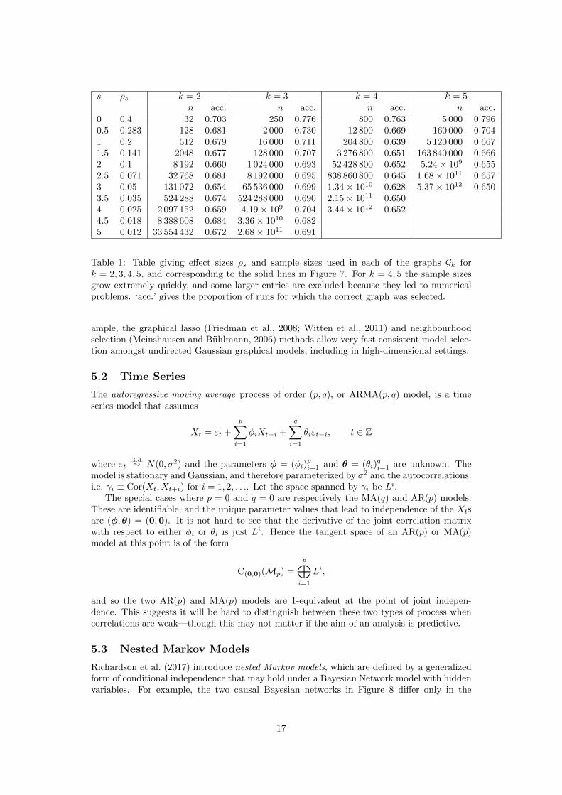
s ρs k = 2 k = 3 k = 4 k = 5n acc. n acc. n acc. n acc.

0 0.4 32 0.703 250 0.776 800 0.763 5 000 0.7960.5 0.283 128 0.681 2 000 0.730 12 800 0.669 160 000 0.7041 0.2 512 0.679 16 000 0.711 204 800 0.639 5 120 000 0.6671.5 0.141 2048 0.677 128 000 0.707 3 276 800 0.651 163 840 000 0.6662 0.1 8 192 0.660 1 024 000 0.693 52 428 800 0.652 5.24× 109 0.6552.5 0.071 32 768 0.681 8 192 000 0.695 838 860 800 0.645 1.68× 1011 0.6573 0.05 131 072 0.654 65 536 000 0.699 1.34× 1010 0.628 5.37× 1012 0.6503.5 0.035 524 288 0.674 524 288 000 0.690 2.15× 1011 0.6504 0.025 2 097 152 0.659 4.19× 109 0.704 3.44× 1012 0.6524.5 0.018 8 388 608 0.684 3.36× 1010 0.6825 0.012 33 554 432 0.672 2.68× 1011 0.691

Table 1: Table giving effect sizes ρs and sample sizes used in each of the graphs Gk fork = 2, 3, 4, 5, and corresponding to the solid lines in Figure 7. For k = 4, 5 the sample sizesgrow extremely quickly, and some larger entries are excluded because they led to numericalproblems. ‘acc.’ gives the proportion of runs for which the correct graph was selected.

ample, the graphical lasso (Friedman et al., 2008; Witten et al., 2011) and neighbourhoodselection (Meinshausen and Buhlmann, 2006) methods allow very fast consistent model selec-tion amongst undirected Gaussian graphical models, including in high-dimensional settings.

5.2 Time Series

The autoregressive moving average process of order (p, q), or ARMA(p, q) model, is a timeseries model that assumes

Xt = εt +

p∑i=1

φiXt−i +

q∑i=1

θiεt−i, t ∈ Z

where εti.i.d.∼ N(0, σ2) and the parameters φ = (φi)

pi=1 and θ = (θi)

qi=1 are unknown. The

model is stationary and Gaussian, and therefore parameterized by σ2 and the autocorrelations:i.e. γi ≡ Cor(Xt, Xt+i) for i = 1, 2, . . .. Let the space spanned by γi be Li.

The special cases where p = 0 and q = 0 are respectively the MA(q) and AR(p) models.These are identifiable, and the unique parameter values that lead to independence of the Xtsare (φ,θ) = (0,0). It is not hard to see that the derivative of the joint correlation matrixwith respect to either φi or θi is just Li. Hence the tangent space of an AR(p) or MA(p)model at this point is of the form

C(0,0)(Mp) =

p⊕i=1

Li,

and so the two AR(p) and MA(p) models are 1-equivalent at the point of joint indepen-dence. This suggests it will be hard to distinguish between these two types of process whencorrelations are weak—though this may not matter if the aim of an analysis is predictive.

5.3 Nested Markov Models

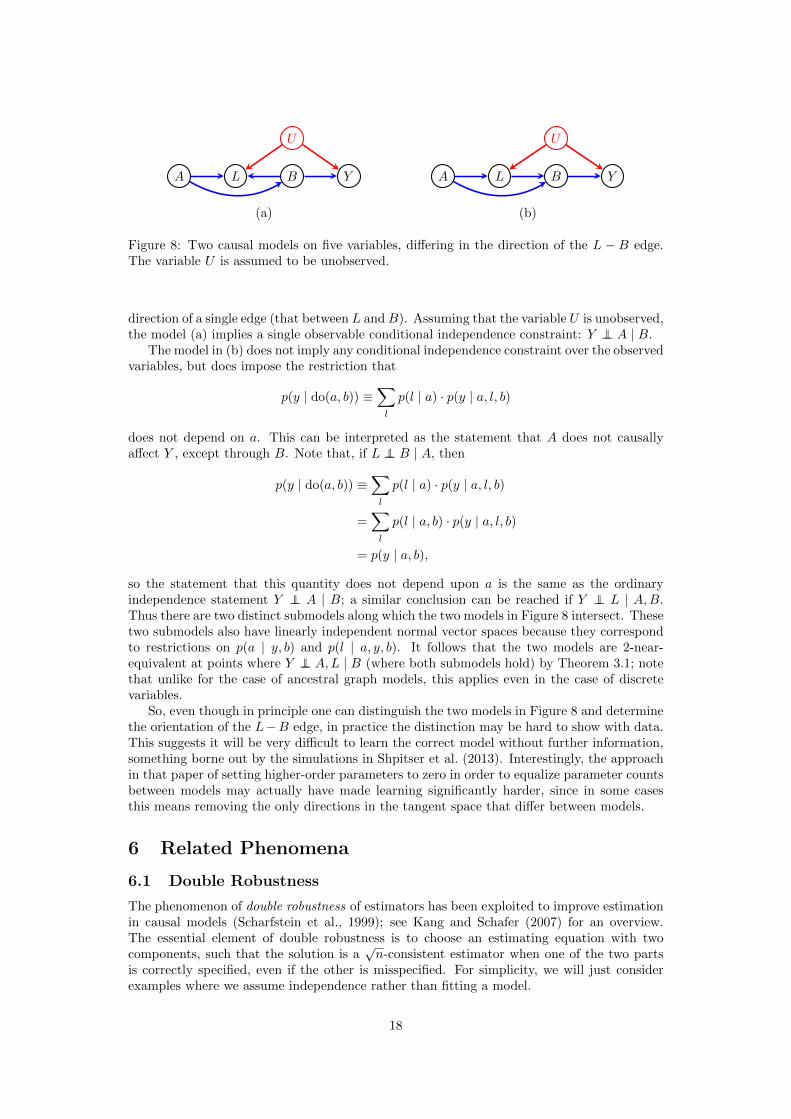
Richardson et al. (2017) introduce nested Markov models, which are defined by a generalizedform of conditional independence that may hold under a Bayesian Network model with hiddenvariables. For example, the two causal Bayesian networks in Figure 8 differ only in the

17

A L B Y

U

(b)

A L B Y

U

(a)

Figure 8: Two causal models on five variables, differing in the direction of the L − B edge.The variable U is assumed to be unobserved.

direction of a single edge (that between L andB). Assuming that the variable U is unobserved,the model (a) implies a single observable conditional independence constraint: Y ⊥⊥ A | B.

The model in (b) does not imply any conditional independence constraint over the observedvariables, but does impose the restriction that

p(y | do(a, b)) ≡∑l

p(l | a) · p(y | a, l, b)

does not depend on a. This can be interpreted as the statement that A does not causallyaffect Y , except through B. Note that, if L ⊥⊥ B | A, then

p(y | do(a, b)) ≡∑l

p(l | a) · p(y | a, l, b)

=∑l

p(l | a, b) · p(y | a, l, b)

= p(y | a, b),

so the statement that this quantity does not depend upon a is the same as the ordinaryindependence statement Y ⊥⊥ A | B; a similar conclusion can be reached if Y ⊥⊥ L | A,B.Thus there are two distinct submodels along which the two models in Figure 8 intersect. Thesetwo submodels also have linearly independent normal vector spaces because they correspondto restrictions on p(a | y, b) and p(l | a, y, b). It follows that the two models are 2-near-equivalent at points where Y ⊥⊥ A,L | B (where both submodels hold) by Theorem 3.1; notethat unlike for the case of ancestral graph models, this applies even in the case of discretevariables.

So, even though in principle one can distinguish the two models in Figure 8 and determinethe orientation of the L−B edge, in practice the distinction may be hard to show with data.This suggests it will be very difficult to learn the correct model without further information,something borne out by the simulations in Shpitser et al. (2013). Interestingly, the approachin that paper of setting higher-order parameters to zero in order to equalize parameter countsbetween models may actually have made learning significantly harder, since in some casesthis means removing the only directions in the tangent space that differ between models.

6 Related Phenomena

6.1 Double Robustness

The phenomenon of double robustness of estimators has been exploited to improve estimationin causal models (Scharfstein et al., 1999); see Kang and Schafer (2007) for an overview.The essential element of double robustness is to choose an estimating equation with twocomponents, such that the solution is a

√n-consistent estimator when one of the two parts

is correctly specified, even if the other is misspecified. For simplicity, we will just considerexamples where we assume independence rather than fitting a model.

18

Consider the simple causal model depicted in Figure 6(c), and suppose we are interestedin the causal effect of a binary variable X on the expectation of Y , but there is a (poten-tially continuous) measured confounder Z. The causal distribution for X on Y is given byp(y | do(x)) =

∑z p(z) · p(y |x, z); this is generally different from the ordinary conditional

p(y |x) =∑z p(z |x) · p(y |x, z).

What happens if we use the ordinary conditional anyway? One can easily check thatp(y |x) = p(y | do(x)) if either X ⊥⊥ Z or Y ⊥⊥ Z | X, and hence the set of distributions whereour estimate is correct contains the union of pointsMX⊥⊥Z ∪MY⊥⊥Z|X . If we apply Theorem3.1 we find that any error in estimating the causal effect will be quadratic in the distancefrom the point where Z ⊥⊥ X,Y .

6.2 Triple Robustness

Another phenomenon known as triple robustness7 is observed in some causal models relatedto mediation (Tchetgen and Shpitser, 2012). In this case, an estimator will be consistentprovided at least two out of three other quantities are correctly specified. Here we introduceanother result related to Theorem 3.1.

Proposition 6.1. Let N1, . . . ,Nm be algebraic submodels containing 0, and let f be a poly-nomial such that f(x) = 0 for any x ∈ Ni ⊂ Θ for i = 1, . . . ,m. Suppose also that the tangentspaces T0(Ni) jointly span Θ. Then, f(x) = O(‖x‖2).

Proof. For any twice differentiable function with f(0) = 0, whichever direction we moveaway from 0 in can be written as a linear combination of directions in the tangent spaces ofsubmodels Ni. It follows that the directional derivative of any such function is zero, in anydirection. Hence f(x) = O(‖x‖2).

In light of this, suppose we have three submodelsM1,M2,M3 each defined by constraintson linearly independent parts of the full model Θ, and such that an estimator is consistent onthe intersection of any two of them. The condition on the definition of the Mi means thattheir normal vector spaces are linearly independent, so any vector is in the tangent space ofat least two such submodels. Their pairwise intersections thus satisfy the conditions of thetheorem, and the error in estimating the relevant parameter is quadratic in the distance tothe joint intersection M1 ∩M2 ∩M3.

6.3 Post-double-Selection

Belloni et al. (2014) consider the problem of estimating a causal effect p(y | do(x)) in thepresence of a high-dimensional measured confounder ZI , I = 1, . . . , p where p n. Wecan try to find a subset S ⊆ I such that S is much smaller than I, and ZS is sufficient tocontrol for the confounding, i.e. p(y | do(x)) =

∑zSp(zS) p(y |x, zS). Formally, this will be

satisfied if we ignore any Zi such that Zi ⊥⊥ X | Z−i or Zi ⊥⊥ Y | X,Z−i. However, in finitesamples selecting variables creates an omitted-variable bias, in which the decision boundaryof whether to drop a particular variable leads to a bias of order O(n−1/2) at some points inthe parameter space.

If we only exclude components of Zi for which both Zi ⊥⊥ X | Z−i and Zi ⊥⊥ Y | X,Z−i,then the order of the bias on our causal estimate is effectively squared and becomes O(n−1);this is because—for the same reason as in the discussion of double robustness—the biasinduced by a component Zi is at most quadratic in the distance of the true distributionfrom the intersection of these two independences. Since this bias is small compared to thesampling variance, it can effectively be ignored; this idea is referred by Belloni et al. (2014)to as post-double-selection, and can be viewed as another consequence of the local geometryof the model.

7Perhaps misleadingly, since it is strictly weaker than double robustness.

19

7 Algorithms for Learning Models with Overlap

Suppose we have a class of models Mi that overlap but are not 1-equivalent: that is, themodels all have different tangent cones. We have seen already that overlapping models placerestrictions on one class of computationally efficient methods, because they cannot be madeconvex. This suggests that a method which attempts to learn the (linear) tangent cone ratherthan selecting the model directly may be computationally advantageous. This can be achievedby learning from a set of ‘surrogate’ models that have the same tangent spaces as the originalmodels, but that do not overlap.

To take a simple example, consider again the graphical models in Figure 2 for binaryvariables. Letting

λXY =1

8

∑x,y,z∈0,1

(−1)|x+y| logP (X = x, Y = y, Z = z),

then the model M2 in (b) consists of the zero parameters: λXY = λXY Z = 0, while (a)involves log-linear parameters over the X,Y -margin M1 : λ′XY = 0. This apparently makesmodel selection tricky because some models involve zeroes of ordinary log-linear parameters,and some of marginal log-linear parameters.

However, one could try replacing M1 with a model that corresponds to the zero of theordinary log-linear parameter, e.g. M′1 : λXY = 0. This has the same tangent space asM1 atthe uniform distribution, and so it is ‘close’ toM1 in a precise sense. This suggests that if wepursued a model selection strategy for ordinary log-linear parameters and learned λXY = 0but λXY Z 6= 0 (i.e. we chose M′1), then we could conclude that this is sufficiently similar toM1 to select this model from the graphical class.

7.1 Model Selection

Define Λi = 〈ei〉 to be the vector space spanned by the ith coordinate axis. Suppose we havea class of regular algebraic models Mi ⊆ Θ ⊆ Rk such that each model has a tangent spaceat θ = 0 defined by a subset of coordinate axes: that is, for each model there is some setc(Mi) ⊆ 1, . . . , k such that

C0(Mi) =⊕

j∈c(Mi)

Λj .

Suppose further that our class of models is such that c(Mi) 6= c(Mj) for any i 6= j. We havealready seen that, if two models overlap, then it may be computationally difficult to learn thecorrect one due to a lack of convexity. We will show that, under certain assumptions aboutthe true parameter being sufficiently close to θ = 0, we can learn the tangent space itself,thereby circumventing the models’ lack of convexity.

Denote the sparsity pattern of a parameter by c(θ) = i : θi 6= 0; then θ ∈ T0(M)implies that c(θ) ⊆ c(T0(M)) = c(M). However, note that θ ∈ M does not imply this, andin general the sparsity patterns of parameters in M is arbitrary.

Suppose we have a model selection procedure which returns a set S estimating S ⊆1, . . . , k such that θS 6= 0 and θSc = 0. We will assume that the procedure is consistent, inthe sense that if θnSc = o(n−1/2) and |θns | = ω(n−1/2) for each s ∈ S, we have P (S = S)→ 1.These conditions are satisfied by many common model selection methods such as BIC, or anL1-penalized selection method with appropriate penalty (and with Fisher information matrixsatisfying certain irrepresentability conditions, Nardi and Rinaldo, 2012).

The following result shows that we can adapt a model selection procedure of this kindto learn models that overlap, by replacing each (possibly non-convex) model of interest by aconvex surrogate model with the same tangent space.

20

Theorem 7.1. Consider a sequence of parameters of the form θn = θ0 + n−γh + O(n−2γ)such that each θn ∈ M; here 1

4 < γ < 12 and hi 6= 0 for any i ∈ c(M). Suppose our model

selection procedure provides a sequence of parameter estimates θn.Then P (c(θn) = c(M))→ 1 as n→∞.

Proof. If i 6∈ c(M) then θni = O(n−2γ) = o(n−1/2) since γ > 14 , while if i ∈ c(M) then

θni = Ω(n−γ) = ω(n−1/2) since γ < 12 . By the conditions on our model selection procedure

then, we have the required consistency.

The condition γ > 14 is to ensure that the bias induced by using the surrogate model is

too small to detect at the specific sample size, and that our procedure will set the relevantparameters to zero. Slower rates of convergence (i.e. 0 < γ ≤ 1

4 ) could also lead to asatisfactory model selection procedure if we were simply to subsample our data or otherwise‘pretend’ that n is smaller than it actually is. If γ > 1

2 , on the other hand, we will not haveasymptotic power to identify the truly non-zero parameters.

Note that P (c(θn) = c(θn)) does not tend to 1, since the sparsity pattern of the trueparameter is not the same as that of the tangent space of the model: it is merely ‘close’ tohaving the correct sparsity.

The assumption that θn tends to 0 at the required rate may seem rather artificial: someassumption of this form is unavoidable, simply because our results only hold in a neighbour-hood of points of intersection. The precise rate at which θn → 0 just needs to be such that‘real’ effects do not disappear faster than we can statistically detect them (i.e. slower thann−1/2 → 0), and that any other effects shrink fast enough that they are taken to be zero.Any more realistic framework would require conditions on the global geometry of the models,and would be extremely challenging to verify.

7.2 Application to Bayesian Networks

Suppose that we have a sequence of binary distributions pn, with ‖pn − p0‖ = O(n−γ) for14 < γ < 1

2 , where p0 is the uniform distribution, and such that each pn is Markov with

respect to a Bayesian network G; assume also that λij = ω(n−1/2) if i, j are adjacent, andλijk = ω(n−1/2) if i → k ← j is an unshielded collider. Then a consistent method todetermine G would be as follows:

• select the model for pn using the log-linear lasso with penalty ν = nδ for some 12 < δ < 1;

• then find the graph. Asymptotically, the sparsity pattern of the log-linear model is thesame as that of the original graph, so this can be done by simply finding the graphwith skeleton given by i − j when λij 6= 0 and orienting unshielded triples as collidersi→ k ← j if and only if λijk 6= 0.

This is far from an optimal approach, but does give an idea of how one might be ableto overcome the non-convexity inherent to overlapping models. The algorithm could also beextended to ancestral graphs, via Theorem 4.5.

8 Discussion

We have proposed that the geometry of two models at points of intersection is a usefulmeasure of how statistically difficult it will be to distinguish between them, and shown thatwhen models’ tangent spaces are not closed under intersection this restricts the possibility ofusing convex methods to perform model selection in the class. We have also given examplesof model classes in which this occurs and noted that in several cases, model selection is indeedknown to be difficult.

We suggest that special consideration should be given in model selection problems towhether or not the class contains models that overlap or are 1-equivalent and—if it does—to

21

whether a smaller and simpler model class can be used instead. Alternatively, additionalexperiments may need to be performed to help distinguish between models. The results inthis paper provide a point of focus for new model selection methods and also for experimentaldesign. If we are able to work with a class of models that is less rich and therefore easier toselect from, then perhaps we ought to. If we cannot, it is useful to know in advance at whatpoints in the parameter space it is likely to be difficult to draw clear distinctions betweenmodels, so that we can power our experiments correctly or just report that we do not knowwhich of several models is correct.

Acknowledgments

We thank Thomas Richardson for suggesting one of the examples, Bernd Sturmfels for point-ing out a problem with a version of Theorem 3.1, as well as several other readers for helpfulcomments. We also acknowledge the very helpful comments of the referees and associateeditor.

References

B. Aragam and Q. Zhou. Concave penalized estimation of sparse Gaussian Bayesian networks.Journal of Machine Learning Research, 16:2273–2328, 2015.

I. A. Beinlich, H. J. Suermondt, R. M. Chavez, and G. F. Cooper. The ALARM monitoringsystem. In J. Hunter, J. Cookson, and J. Wyatt, editors, Proceedings of AIME 89: SecondEuropean Conference on Artificial Intelligence in Medicine., pages 247–256. Springer BerlinHeidelberg, 1989.

A. Belloni, V. Chernozhukov, and C. Hansen. Inference on treatment effects after selectionamong high-dimensional controls. The Review of Economic Studies, 81(2):608–650, 2014.

W. P. Bergsma and T. Rudas. Marginal models for categorical data. Annals of Statistics, 30(1):140–159, 2002.

C. M. Bishop. Pattern recognition and machine learning. Springer, 2007.

J. Bochnak, M. Coste, and M.-F. Roy. Real algebraic geometry, volume 36. Springer Science& Business Media, 2013.

L. Breiman. Statistical modeling: The two cultures (with discussion). Statistical Science, 16(3):199–231, 2001.

P. Buhlmann and S. van de Geer. Statistics for High-Dimensional Data: Methods, Theoryand Applications. Springer, 2011.

P. Buhlmann, J. Peters, J. Ernest, et al. CAM: Causal additive models, high-dimensionalorder search and penalized regression. Annals of Statistics, 42(6):2526–2556, 2014.

D. M. Chickering. Learning Bayesian networks is NP-complete. In Learning from data, pages121–130. Springer, 1996.

L. Conlon. Differentiable manifolds, second edition. Birkhauser, 2008.

D. Cox, J. Little, and D. O’Shea. Ideals, Varieties, and Algorithms: An Introduction toComputational Algebraic Geometry and Commutative Algebra. Springer, third edition,2008.

D. R. Cox. Role of models in statistical analysis. Statistical Science, 5(2):169–174, 1990.

M. Drton. Likelihood ratio tests and singularities. Annals of Statistics, 37(2):979–1012, 2009a.

22

M. Drton. Discrete chain graph models. Bernoulli, 15(3):736–753, 2009b.

M. Drton and S. Sullivant. Algebraic statistical models. Statistica Sinica, 17(4):1273–1297,2007.

M. Drton, B. Sturmfels, and S. Sullivant. Lectures on algebraic statistics, volume 39. SpringerScience & Business Media, 2008.

R. J. Evans. Smoothness of marginal log-linear parameterizations. Electronic Journal ofStatistics, 9(1):475–491, 2015.

M. Ferrarotti, E. Fortuna, and L. Wilson. Local approximation of semialgebraic sets. Annalidella Scuola Normale Superiore di Pisa, 1:1–11, 2002.

J. Friedman, T. Hastie, and R. Tibshirani. Sparse inverse covariance estimation with thegraphical lasso. Biostatistics, 9(3):432–441, 2008.

F. Fu and Q. Zhou. Learning sparse causal Gaussian networks with experimental intervention:regularization and coordinate descent. Journal of the American Statistical Association, 108(501):288–300, 2013.

J. Gu, F. Fu, and Q. Zhou. Adaptive penalized estimation of directed acyclic graphs fromcategorical data. arXiv preprint arXiv:1403.2310, 2014.

J. D. Y. Kang and J. L. Schafer. Demystifying double robustness: A comparison of alternativestrategies for estimating a population mean from incomplete data. Statistical Science, 22(4):523–539, 2007.

S. L. Lauritzen and N. Wermuth. Graphical models for associations between variables, someof which are qualitative and some quantitative. Annals of Statistics, 17(1):31–57, 1989.

N. Meinshausen and P. Buhlmann. High-dimensional graphs and variable selection with thelasso. Annals of Statistics, 34(3):1436–1462, 2006.

Y. Nardi and A. Rinaldo. The log-linear group-lasso estimator and its asymptotic properties.Bernoulli, 18(3):945–974, 2012.

Y. Ni, F. C. Stingo, and V. Baladandayuthapani. Bayesian nonlinear model selection for generegulatory networks. Biometrics, 71(3):585–595, 2015.

Pearl. Causality: models, reasoning and inference. CUP, second edition, 2009.

T. S. Richardson and P. Spirtes. Ancestral graph Markov models. Annals of Statistics, 30(4):962–1030, 2002.

T. S. Richardson, R. J. Evans, J. M. Robins, and I. Shpitser. Nested Markov properties foracyclic directed mixed graphs. arXiv:1701.06686, 2017.

G. V. Rocha, X. Wang, and B. Yu. Asymptotic distribution and sparsistency for `1-penalizedparametric M-estimators with applications to linear SVM and logistic regression. arXivpreprint arXiv:0908.1940, 2009.

T. Rudas, W. P. Bergsma, and R. Nemeth. Marginal log-linear parameterization of conditionalindependence models. Biometrika, 97:1006–1012, 2010.

D. O. Scharfstein, A. Rotnitzky, and J. M. Robins. Rejoinder to “adjusting for nonignorabledrop-out using semiparametric nonresponse models”. Journal of the American StatisticalAssociation, 94(448):1135–1146, 1999.

S. Shimizu, P. O. Hoyer, A. Hyvarinen, and A. Kerminen. A linear non-Gaussian acyclicmodel for causal discovery. The Journal of Machine Learning Research, 7:2003–2030, 2006.

23

A. Shojaie and G. Michailidis. Penalized likelihood methods for estimation of sparse high-dimensional directed acyclic graphs. Biometrika, 97(3):519–538, 2010.

I. Shpitser, R. Evans, T. Richardson, and J. Robins. Sparse nested Markov models withlog-linear parameters. In UAI-2013, pages 576–585, 2013.

A. Skrondal and S. Rabe-Hesketh. Generalized latent variable modeling: Multilevel, longitu-dinal, and structural equation models. Chapman & Hall/CRC Press, 2004.

P. Spirtes, C. Glymour, and R. Scheines. Causation, Prediction, and Search. MIT Press,second edition, 2000.

E. J. T. Tchetgen and I. Shpitser. Semiparametric theory for causal mediation analysis:efficiency bounds, multiple robustness, and sensitivity analysis. Annals of Statistics, 40(3):1816, 2012.

R. Tibshirani. Regression shrinkage and selection via the lasso. Journal of the Royal StatisticalSociety, Series B, 58:267–288, 1996.

C. Uhler, G. Raskutti, P. Buhlmann, and B. Yu. Geometry of the faithfulness assumption incausal inference. Annals of Statistics, 41(2):436–463, 2013.

A. W. van der Vaart. Asymptotic Statistics. Cambridge University Press, 1998.

D. M. Witten, J. H. Friedman, and N. Simon. New insights and faster computations for thegraphical lasso. Journal of Computational and Graphical Statistics, 20(4):892–900, 2011.

J. Zhang. On the completeness of orientation rules for causal discovery in the presence oflatent confounders and selection bias. Artificial Intelligence, 172(16):1873–1896, 2008.

P. Zwiernik, C. Uhler, and D. Richards. Maximum likelihood estimation for linear Gaussiancovariance models. Journal of the Royal Statistical Society, Series B, 79(4):1269–1292,2017.

A Technical Results

A.1 Asymptotics

We start with the definition of differentiability in quadratic mean.

Definition A.1. Let (pθ : θ ∈ Θ) be a class of densities with respect to a measure µ indexedby some open Θ ⊆ Rk. We say that this class is differentiable in quadratic mean (DQM) atθ if there exists a vector ˙(θ) ∈ Rk such that∫ [

√pθ+h −

√pθ −

1

2hT ˙(θ)

√pθ

]2

dµ = o(‖h‖2).

Recall also our definition of a model that is doubly DQM.Definition 2.8 Say that pθ is doubly differentiable in quadratic mean (DDQM) at θ ∈ Mif for any sequences h, h→ 0, we have∫ (

√pθ+h −

√pθ+h −

1

2(h− h)T ˙(θ + h)

√pθ+h

)2

dµ = o(‖h− h‖2).

Recall also that DDQM reduces to DQM in the special case h = 0, and that (by symmetry)we could replace ˙

θ+h√pθ+h by ˙

θ+h√pθ+h. On the other hand it is strictly stronger than

DQM at θ.

24

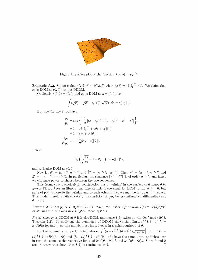
Figure 9: Surface plot of the function f(x, y) = xy1/3.

Example A.2. Suppose that (X,Y )T ∼ N(η, I) where η(θ) = (θ1θ1/32 , θ2). We claim that

pθ is DQM at (0, 0) but not DDQM.Obviously η(0, 0) = (0, 0) and pη is DQM at η = (0, 0), so∫

(√pη −

√p0 − ηT ˙(0)

√p0)2 dη = o(‖η‖2).

But now for any θ, we have

pθp0

= exp

−1

2

[(x− η1)2 + (y − η2)2 − x2 − y2

]= 1 + xθ1θ

1/32 + yθ2 + o(‖θ‖)

= 1 + yθ2 + o(‖θ‖)√pθp0

= 1 +1

2yθ2 + o(‖θ‖).

Hence

E0

(√pθp0− 1− θ2Y

)2

= o(‖θ‖2),

and pθ is also DQM at (0, 0).Now let θn = (n−1/6, n−1/2) and θn = (n−1/6,−n1/2). Then ηn = (n−1/3, n−1/2) and

ηn = (−n−1/3,−n−1/2). In particular, the sequence ‖ηn − ηn‖ is of order n−1/3, and hencewe will have power to choose between the two sequences.

This (somewhat pathological) construction has a ‘wrinkle’ in the surface that maps θ toη—see Figure 9 for an illustration. The wrinkle is too small for DQM to fail at θ = 0, butpairs of points close to the wrinkle and to each other in θ space may be far apart in η space.This model therefore fails to satisfy the condition of

√pθ being continuously differentiable at

θ = (0, 0).

Lemma A.3. Let pθ be DDQM at θ ∈ Θ. Then, the Fisher information I(θ) ≡ E ˙(θ) ˙(θ)T

exists and is continuous in a neighbourhood of θ ∈ Θ.

Proof. Since pθ is DDQM at θ it is also DQM, and hence I(θ) exists by van der Vaart (1998,Theorem 7.2). In addition, the symmetry of DDQM shows that limt→0 h

T I(θ + th)h =hT I(θ)h for any h, so this matrix must indeed exist in a neighbourhood of θ.

By the symmetry property noted above,∫ [

(h− th)T ˙(θ + t2h)√pθ+t2h

]2dµ = (h −

th)T I(θ + t2h)(h − th) and (h − th)T I(θ + th)(h − th) have the same limit, and these arein turn the same as the respective limits of hT I(θ + t2h)h and hT I(θ + th)h. Since h and hare arbitrary, this shows that I(θ) is continuous at θ.

25

We now prove Theorem 2.9, closely following the proof of Theorem 7.2 of van der Vaart(1998).

Proof of Theorem 2.9. Let pn and pn respectively denote pθ+hnand pθ+hn

. By DDQM we

have that√n(√pn−√pn) − 1

2kT ˙(θ + hn)

√pn converges in quadratic mean to 0; since the

second term is bounded in squared expectation (given by kT I(θ+ hn)k/4) so is the first, andhence nγ(

√pn−√pn)→ 0 in quadratic mean for any γ < 1

2 .

Let gn = kT ˙(θ + hn). Note that DDQM implies that 12gn√pn has the same limit as√

n(√pn−√pn). By continuity of the inner product, we have

limn

Eθ+hngn = lim

n

∫gnpn dµ

= limn

∫1

2gn√pn2√pn dµ

= limn

√n

∫(√pn −

√pn)(√pn +

√pn) dµ

= limn

√n

∫(pn − pn) dµ

= 0,

since∫

(pn − pn) dµ = 1− 1 = 0 for all densities pn, pn.

Let Wni = 2(√pn/pn(Xi)− 1) where Xi ∼ pn. Then

nEWni = 2n

∫ √pnpn dµ− 2n = −n

∫(√pn −

√pn)2 dµ

which, by the DDQM condition, has the same limit as

−1

4kT(Eθ+hn

˙(θ + hn)T ˙(θ + hn))k = −1

4kT I(θ + hn)k.

Then

Varθ+hn

(∑i

Wni −1√n

∑i

gn(Xi)

)≤ Eθ+hn

(√nWni − gn(Xi)

)2(3)

=

∫ (√nWni − gn(Xi)

)2pn dµ

=

∫ (√n2(√pn/pn − 1)− kT ˙(θ + hn)

)2

pn dµ

=

∫4

(√n(√pn −

√pn)− 1

2kT ˙(θ + hn)

√pn

)2

dµ

= o(1)

by DDQM. It follows from all this that the sequence of random variables∑i

Wni −1√n

∑i

gn(Xi) +1

4kT I(θ + hn)k

has mean and variance tending to zero, and hence they converge to zero in probability.Using a Taylor expansion, we obtain

log

n∏i=1

pθ+hn

pθ+hn

(Xi) = 2

n∑i=1

log(1 +Wni/2)

=

n∑i=1

Wni −1

4

n∑i=1

W 2ni +

1

2

n∑i=1

W 2niR(Wni) (4)

26

for some function R such that limx→0R(x) = 0. By the right-hand side of (3), we havenW 2

ni = gn(Xi)2 + Ani for some Ani such that E|Ani| → 0, and hence An = n−1

∑iAni

converges in probability to 0. Then∑i

W 2ni − n−1

∑i

gn(Xi)2 = An = op(1).

We also have

P (maxi|Wni| > ε

√2) ≤ nP (|Wni| > ε

√2)

≤ nP (gn(Xi)2 > nε2) + nP (|Ani| > nε2)

≤ ε−2Egn(Xi)2Ign(Xi)2>nε2 + ε−2E|Ani|.

We already have E|Ani| → 0, and since Egn(Xi)2 = kT I(θ + hn)k is continuous (and hence

bounded) by Lemma A.3, the first term also tends to 0. It follows that maxi |Wni| =op(1) and thus maxi |R(Wni)| = op(1). Note therefore that the final term is bounded bymax1≤i≤n |R(Wni)| ·

∑ni=1W

2ni = op(1)Op(1) which converges to zero in probability.

Putting this back into (4) gives

log

n∏i=1

pθ+hn

pθ+hn

(Xi) =

n∑i=1

Wni −1

4kT I(θ + hn)k + op(1).

We then directly obtain

`(θ + hn)− `(θ + hn) =1√n

∑i

gn(Xi)−1

2kT I(θ + hn)k + op(1)

=1√nkT ˙(θ + hn)− 1

2kT I(θ + hn)k + op(1).

Using the fact that I(·) is continuous at θ then gives the required result.

Sufficient conditions for DQM are given in Lemma 7.6 of van der Vaart (1998); in fact,these conditions are also sufficient for DDQM.

Lemma A.4. Assume that θ 7→ sθ(x) :=√pθ(x) is µ-almost everywhere continuously dif-

ferentiable, and that the matrix I(θ) :=∫

(pθ/pθ)(pTθ /pθ)pθ dµ has well-defined continuous

entries. Then pθ is DDQM.

Proof. We follow the same proof method as Lemma 7.6 in van der Vaart (1998). By the chainrule, pθ is also differentiable with pθ = 2sθ sθ, and hence sθ = 1

2 (pθ/pθ)√pθ.

Since θ 7→ sθ(x) is continuously differentiable (assuming for now that x excludes the setof measure zero on which this fails), we can write

sθ+th − sθ+tgt

= (h− g)T sθ+t(g+u(h−g)).

for some u ∈ [0, 1] by the mean value theorem.By Cauchy-Schwarz and Fubini, we have∫ (

sθ+th − sθ+tgt

)2

dµ ≤∫ ∫ 1

0

((h− g)T sθ+t(g+u(h−g))

)2du dµ

=1

4

∫ 1

0

(h− g)T I(θ + t(g + u(h− g)))(h− g) du

−→ 1

4(h− g)T I(θ)(h− g);

here we have used the continuity of I(·). Continuous differentiability of s(·) shows thatt−1(sθ+th− sθ+tg)− (h− g)T sθ+tg → 0 pointwise, and hence its integral converges to zero byProposition 2.29 of van der Vaart (1998).

27

We remark that Lemmas A.3 and A.4 show a close correspondence between continuity ofthe Fisher information and DDQM.

It is a standard result that the conditions of Lemma A.4 are satisfied by an exponentialfamily provided that θ is in the interior of the natural parameter space.

A.2 Proof of Theorem 2.10

Proof. Assume x = 0 without loss of generality. Given hn ∈ S1 with hn → 0, and the factthat S1 and S2 are c-equivalent at 0, there exists a sequence hn = hn + o(εcn) with hn ∈ S2.Now, choosing εn = ‖hn‖ which also tends to 0, we obtain hn = hn + o(‖hn‖c).

Now, if hn = O(n−12c ), then hn−hn = o(n−1/2), which gives the required result. A similar

argument holds for c-near-equivalence, giving hn − hn = O(n−1/2).

A.3 Proof of Theorem 3.1

Lemma A.5. Let the conditions of Theorem 3.1 be satisfied with m ≥ 2. Then M1 and M2

have the same dimension and tangent space at θ.

Proof. We have that Tθ(M1 ∩ Ni) = Tθ(M1) ∩ Tθ(Ni) for i = 1, 2. Since N1 and N2 havedisjoint normal spaces, it follows that

Tθ(M1) = Tθ(M1) ∩ (Tθ(N1) + Tθ(N2))

= Tθ(M1 ∩N1) + Tθ(M1 ∩N2)

= Tθ(M2 ∩N1) + Tθ(M2 ∩N2)

= Tθ(M2) ∩ (Tθ(N1) + Tθ(N2))

= Tθ(M2).

Since M1, M2 are regular at θ, this completes the proof.

The proof below makes modest use of differential geometry; the basics may be found inConlon (2008).

Proof of Theorem 3.1. We choose θ = 0 for convenience. The result is clear for m = 1, soassume m ≥ 2. By Lemma A.5, M1 and M2 share a common dimension and tangent spaceat 0. Since M1,M2 are Dm surfaces at 0, they can each be locally represented by a Dm

parametric function, say φ1, φ2 : U → Rk. Assume that φ1(0) = φ2(0) = 0, and that thesefunctions share a derivative at 0 with respect to u ∈ U .

Choose φ1 so that φ1(u) = (u, 0) ∈ Rd×Rk−d, by the constant rank theorem (Conlon, 2008,Theorem 2.4.6). Note this means that φ2(u) = (u,O(‖u‖2)) by the definition of the tangentspace and the fact that φ2 is at least D2. Also set φ−1

1 (A) = φ−12 (A) for all A ⊆ Mj ∩ Ni;

then for each u : φ1(u) ∈M1 ∩Ni we have φ2(u) = (u, 0).By the implicit function theorem, each of the remaining k − d coordinates of φ2 can be

written as a Dm function of the first d. By a further invertible Dm transformation, we canensure that φ1(u), φ2(u) ∈ Ni whenever uci−1+1 = · · · = uci = 0 (where ci − ci−1 is thecodimension of Mj ∩Ni in Mj).

Note that this means that not only is ∂φ1(0)∂ua

= ∂φ2(0)∂ua

for all a, but indeed ∂m−1φ1(0)∂ua1 ···∂uam−1

=

∂m−1φ2(0)∂ua1

···∂uam−1for all a1, . . . , am−1, because there could still be some i ∈ 1, . . . ,m such that

uci−1+1 = · · · = uci = 0; therefore we are still (potentially) in at least one of the m submodels,

and φ−11 (y) = φ−1

2 (y) holds at this point.It follows that the Taylor expansions of φ1 and φ2 at 0 to order m− 1 are identical, and

the first term in which there is any difference will be of the form

1

m!ua1 · · ·uam

∂mφj(0)

∂ua1 · · · ∂uam,

28

where each ai ∈ ci−1 + 1, . . . , ci. As a consequence of the product ua1 · · ·uam , it followsthat ‖φ1(u)− φ2(u)‖ = O(‖u‖m), and hence M1 and M2 are m-near-equivalent.

B Log-Linear Parameters

Let V be a finite set, and define the log-linear design matrix as a 2|V |×2|V | matrix with rowsand columns indexed by subsets of V , such that

MA,B = (−1)|A∩B|.

We denote the Bth column (or equivalently row) of M by MB . Note that

MB =⊙v∈B

Mv,

where denotes the Hadamard (or point-wise) product. As an example, here is a log-lineardesign matrix for three items.

M =

1 1 1 1 1 1 1 11 −1 1 −1 1 −1 1 −11 1 −1 −1 1 1 −1 −11 −1 −1 1 1 −1 −1 11 1 1 1 −1 −1 −1 −11 −1 1 −1 −1 1 −1 11 1 −1 −1 −1 −1 1 11 −1 −1 1 −1 1 1 −1

∅121, 231, 32, 31, 2, 3

For example, the fourth column of M is M1,2 and is given by the pointwise product of thesecond and third columns M1 and M2. Note also that M is involutory—that is, its own

inverse—up to a constant: M−1 = 2−|V |M .Let XV = (Xv)v∈V be a vector of binary random variables. We abbreviate the event

Xv = 0 for all v ∈ C to 0C , and similarly Xv = 1 for all v ∈ C to 1C . Let ηA =log p(1A, 0V \A). Then we define the log-linear parameters via the identities

η = Mλ, λ = M−1η,

Letting p = (p(xV ) : xV ∈ XV ), assumed to be ordered in the same way as η so that η = log p,we have

∂λ

∂p=∂λ

∂η

∂η

∂p= M−1(diag p(xV ))−1.

Of interest to us is the connection between log-linear parameters within different marginaldistributions, known as marginal log-linear parameters (Bergsma and Rudas, 2002). Denotethe log-linear parameters within a marginal distribution XK by λK ≡ (MK)−1 log p(xK),where MK is the appropriate restriction of M to rows and columns indexed by subsets ofK. We continue to denote the ordinary log-linear parameter associated with a particularinteraction set A by λA = λVA .

Lemma B.1. The derivative of the parameter λKA (with respect to p) lies in the span of thederivatives of λVA , . . . , λ

VV if XK ⊥⊥ XV \K . If K = A, then the converse also holds.

Additionally, if p(xV ) is uniform then λKA and λVA have the same derivative MA.

Proof. Let xV = (1B , 0V \B). We have

∂λKA∂p(xV )

=MA,B

2|K|p(xK)

and∑

C⊆V \A

αC∂λVAC∂p(xV )

=MA,B

2|V |p(xV )

∑C⊆V \A

αCMC,B (5)

29

since MA∪C,B = MA,B ·MC,B . For the derivatives∂λK

A

∂p to lie in the span of the derivatives∂λV

AC

∂p we need to find αC to solve

MA,B

2|V |p(xV )

∑C⊆V \A

αCMC,B =MA,B

2|K|p(xK)

or equivalently ∑C⊆V \A

αCMC,B = 2|V \K|p(xV \K |xK) (6)

for each xV . If XV \K ⊥⊥ XK this becomes∑C⊆V \K αCMC,B = 2|V \K|p(xV \K), which has

a solution because it amounts to 2|V \K| linearly independent equations in 2|V \A| ≥ 2|V \K|

variables.In the case that K = A, note that there are precisely as many variables as equations,

and since the coefficients MC,B expression given on the left of (6) do not vary with xK (sinceC ∩K = ∅), it is necessary for XV \K ⊥⊥ XK in order for a solution to exist. For A ⊂ K asimilar argument shows that XV \K ⊥⊥ XD | XK\D for some D ⊂ K with |D| ≤ |K \ A| issufficient.

If p(xV ) is uniform, then note that the derivative of λKA does not depend upon K.

Since the map from λ to p is a smooth one, this yields us the following Corollary.

Corollary B.2. If ε ≡ ‖p− p0‖ for p0 under which all variables are uniform, then

λKA = λLA +O(ε2).

B.1 Log-Linear Models are Algebraic

Note that a log-linear model is algebraic, since λA = c if and only if∏‖xA‖1 even

p(xA, xV \A)− ec2|V | ∏‖xA‖1 odd

p(xA, xV \A) = 0.

Hence they are defined by the zeroes of polynomials in p.

C Ancestral Graphs

Proof of Theorem 4.5. Let G be a graph with vertices V . We can parameterize the binaryprobability simplex using log-linear parameters λK for ∅ 6= K ⊆ V (see Appendix B fordetails). We consider the tangent space of the model at the uniform distribution; that is, atλK = 0 for every K.

The conditional independenceXa ⊥⊥ Xb | XC is equivalent to the λ′abD = 0 for eachD ⊆ C,where λ′K are the log-linear parameters for the marginal distribution over Xa, Xb, XC (Rudaset al., 2010). However, within δ of the uniform distribution we have λ′K = λK + O(δ2) (seeCorollary B.2). Hence the constraint to the tangent cone imposed by λ′abD = 0 is the sameas that imposed by λabD = 0 for each D ⊆ C.

Now, two MAGs are Markov equivalent if and only if they have the same adjacencies,unshielded colliders, and discriminating paths (e.g. Zhang, 2008, Proposition 2). If theydiffer in adjacencies (say i, j), then a log-linear parameter λij will appear in the tangent coneof one model but not the other. If they differ in an unshielded collider i ∗→ k ←∗ j then inone model λijk = 0 but in the other this direction is not restricted. The same holds for adiscriminating path between i and j for a potential collider k.

30

Remark C.1. Note that this proof also demonstrates that the skeleton of the graph is deter-mined solely by the two-way interaction parameters, and that the remainder of the model canbe deduced entirely from the three-way interaction parameters. This suggests that it mightbe possible to develop a model selection procedure using only this information, something wedo in Section 7. It also illustrates that in cases with strong three-way interactions it shouldbe easier to learn the correct model rather than just the correct skeleton. A ‘noisy-OR’ modelwould, for example, have the desired property. The well known ALARM dataset (Beinlichet al., 1989) has strong interaction effects and is—at least in part for this reason—consideredto be relatively easy to learn.

Proof of Proposition 4.6. We claim that the spaces spanned by λik and λjk are contained inthe tangent cones of both models, but not of their intersection; the first claim follows fromTheorem 4.5. For the second, if Xk is binary then λ′ij = λij = 0 if and only if either λik = 0or λjk = 0 (see Drton et al., 2008, Example 3.1.7). Clearly then directions in which they areboth non-zero will not appear in the intersection model.

Remark C.2. Note that these results can easily be extended to a general finite discrete case,though the notation becomes rather cumbersome. In particular, suppose that the statespaceis XV =

∏v∈V Xv for some finite sets Xv. In this case λA represents a collection of parameters

of dimension∏a∈A(|Xa| − 1); these are redundant whenever some xa is equal to a suitable

reference value (say 0a ∈ Xa), since they can be inferred from the remaining values.Then we define

λA(xA) = |XV |−1∑

yV ∈XV

log p(yV )∏v∈A

(|Xv|1xv=yv − 1).

Hence λ∅ = |XV |−1∑yV

log p(yV ) and

λ1(x1) = |XV |−1∑

yV ∈XV

(|X1|1x1=y1 − 1) log p(yV ),

for example. The results in Section 4 still hold with these parameters at analogous locations.Now, in the case of Proposition 4.6, the same result will hold even ifXk is not binary. Evans

(2015, Theorem 3.1) shows that λAkij = λAij+g(λk|A), where g = 0 whenever Xk ⊥⊥ Xl | XA\lfor any l ∈ V . This means that Xk ⊥⊥ Xi | XA\i or Xk ⊥⊥ Xj | XA\j are included in theintersections of the two models. Further, one can check that the models are not identical, sinceadding ε > 0 to P (XA = xA, Xk = xk) and subtracting it from P (XA = xA, Xk = x′k) will notchange the fact that Xi ⊥⊥ Xj | XA\i,j, but we will no longer have Xi ⊥⊥ Xj | XA\i,j, Xk.It follows that the two models overlap by Theorem 3.3.

D Example: Discrete LWF Chain Graphs

Example D.1. Consider the graphs shown in Figure 10. Interpreted using the Lauritzen-Frydenberg-Wermuth (LWF) Markov property (Lauritzen and Wermuth, 1989), these threegraphs all represent distinct models. The graph in (a) satisfies the usual Markov property forundirected graphs:

X1 ⊥⊥ X4 | X2, X3, X2 ⊥⊥ X3 | X1, X4.

The graphs in (b) and (c) satisfy these independences, as well as the respective independencesX1 ⊥⊥ X2 (in the case of (b)), and X1 ⊥⊥ X2 | X3, X4 for (c). These two additional constraintsare generally distinct, but they coincide if any of the three remaining edges are not present:i.e. if any of the conditional independences

X1 ⊥⊥ X3 | X2, X4, X3 ⊥⊥ X4 | X1, X2, X2 ⊥⊥ X4 | X1, X3,

31

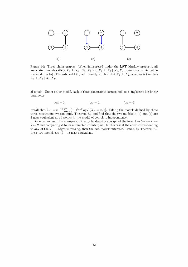
1 2

3 4

(a)

1 2

3 4

(b)

1 2

3 4

(c)

Figure 10: Three chain graphs. When interpreted under the LWF Markov property, allassociated models satisfy X1 ⊥⊥ X4 | X2, X3 and X2 ⊥⊥ X3 | X1, X4; these constraints definethe model in (a). The submodel (b) additionally implies that X1 ⊥⊥ X2, whereas (c) impliesX1 ⊥⊥ X2 | X3, X4.

also hold. Under either model, each of these constraints corresponds to a single zero log-linearparameter:

λ13 = 0, λ34 = 0, λ24 = 0

[recall that λA := 2−|V |∑xV

(−1)|xA| logP (XV = xV )]. Taking the models defined by thesethree constraints, we can apply Theorem 3.1 and find that the two models in (b) and (c) are3-near-equivalent at all points in the model of complete independence.

One can extend this example arbitrarily by drawing a graph of the form 1→ 3− 4− · · ·−k ← 2 and comparing it to its undirected counterpart. In this case if the effect correspondingto any of the k − 1 edges is missing, then the two models intersect. Hence, by Theorem 3.1these two models are (k − 1)-near-equivalent.

32