Model reduction for chemical reaction networks

•First •Prev •Next •Go To •Go Back •Full Screen •Close •Quit 1

Model reduction for chemical reaction networks

• Formulating Markov models

• Reaction networks

• Scaling limit

• Multiscale models

• General approaches to averaging

• Michaelis-Menten equation

• Forcing onto a lower dimensional manifold

• Appendix

• References

• Abstract


Intensities for continuous-time Markov chains

Assume X is a continuous time Markov chain in E ⊂ Zd. The Q-matrix, Q = {qkl},for the chain gives

P{X(t+ ∆t) = l|X(t) = k} ≈ qkl∆t, k 6= l ∈ E,

and hence

E[f(X(t+ ∆t))− f(X(t))|FXt ] ≈

∑l

qX(t),l(f(l)− f(X(t))∆t ≡ Af(X(t))∆t

Alternative notation: Define βl(k) = qk,k+l. Then

Af(k) =∑

l

βl(k)(f(k + l)− f(k))


Martingale problems

≈ is made precise by the requirement that

f(X(t))− f(X(0))−∫ t

0

Af(X(s))ds

be a {FXt }-martingale for f in an appropriate domain D(A).

X is called a solution of the martingale problem for A.

Note that a change of time scale corresponds to multiplying the generator by theappropriate constant.

f(X(ρt))− f(X(0))−∫ ρt

0

Af(X(s))ds

= f(X(ρt))− f(X(0))−∫ t

0

ρAf(X(ρs))ds


Time change equation

X(t) = X(0) +∑

l

lNl(t)

where Nl(t) is the number of jumps of l at or before time t. Nl is a counting processwith intensity (propensity in the chemical literature) βl(X(t)), that is,

Nl(t)−∫ t

0

βl(X(s))ds

is a martingale. Consequently, we can write

Nl(t) = Yl(

∫ t

0

βl(X(s))ds),

where the Yl are independent, unit Poisson processes, and

X(t) = X(0) +∑

l

lYl(

∫ t

0

βl(X(s))ds).


Reaction networks

Standard notation for chemical reactions

A+B ⇀ C

is interpreted as “a molecule of A combines with a molecule of B to give a moleculeof C.”

A+B C

means that the reaction can go in either direction, that is, a molecule of C candissociate into a molecule of A and a molecule of B

We consider a network of reactions involving m chemical species, A1, . . . , Am.

m∑i=1

νikAi ⇀m∑

i=1

ν ′ikAi

where the νik and ν ′ik are nonnegative integers


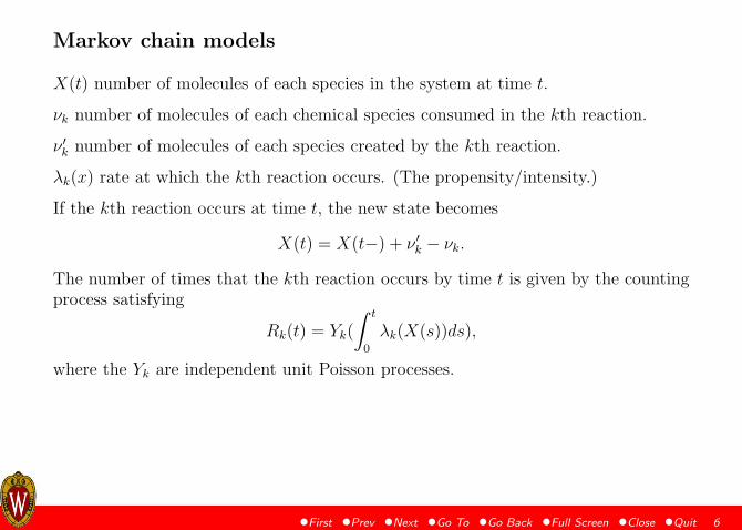
Markov chain models

X(t) number of molecules of each species in the system at time t.

νk number of molecules of each chemical species consumed in the kth reaction.

ν ′k number of molecules of each species created by the kth reaction.

λk(x) rate at which the kth reaction occurs. (The propensity/intensity.)

If the kth reaction occurs at time t, the new state becomes

X(t) = X(t−) + ν ′k − νk.

The number of times that the kth reaction occurs by time t is given by the countingprocess satisfying

Rk(t) = Yk(

∫ t

0

λk(X(s))ds),

where the Yk are independent unit Poisson processes.


Equations for the system state

The state of the system satisfies

X(t) = X(0) +∑

k

Rk(t)(ν′k − νk)

= X(0) +∑

k

Yk(

∫ t

0

λk(X(s))ds)(ν ′k − νk) = (ν ′ − ν)R(t)

ν ′ is the matrix with columns given by the ν ′k.

ν is the matrix with columns given by the νk.

R(t) is the vector with components Rk(t).


Rates for the law of mass action

For a binary reaction A1 + A2 ⇀ A3 or A1 + A2 ⇀ A3 + A4

λk(x) = κkx1x2

For A1 ⇀ A2 A1 ⇀ A2 + A3,λk(x) = κkx1

For 2A1 ⇀ A2,λk(x) = κkx1(x1 − 1)

For a binary reaction A1 + A2 ⇀ A3, the rate should vary inversely with volume, soit would be better to write

λNk (x) = κkN

−1x1x2 = Nκkz1z2,

where classically, N is a scaling parameter taken to be the volume of the system timesAvogadro’s number and zi = N−1xi is the concentration in moles per unit volume.Note that unary reaction rates also satisfy

λk(x) = κkxi = Nκkzi.


Classical scaling limit

Setting CN(t) = N−1X(t)

CN(t) = CN(0) +∑

k

N−1Yk(

∫ t

0

λNk (X(s))ds)(ν ′k − νk)

≈ CN(0) +∑

k

N−1Yk(N

∫ t

0

λk(CN(s))ds)(ν ′k − νk)

The law of large numbers for the Poisson process implies N−1Y (Nu) ≈ u,

CN(t) ≈ CN(0) +∑

k

∫ t

0

κk

∏i

CNi (s)νik(ν ′k − νk)ds,

which in the large volume limit gives the classical deterministic law of mass action

C(t) =∑

k

κk

∏i

Ci(t)νik(ν ′k − νk) ≡ F (C(t)).


A multiscale model [1]

Take N to be of the order of magnitude of the abundance of the most abundantspecies in the system.

For each species i, 0 ≤ αi ≤ 1 and

Zi(t) = N−αiXi(t).

αi should be selected so that Zi = O(1).

The rate constants may also scale κ′k = κkNγk , so for a binary reaction

κ′kxixj = Nγk+αi+αjκkzizj

Select βk so that λ′k(x) = Nβkλk(z), where λk(z) = O(1) for all (most?) relevantvalues of z.

The model becomes

Zi(t) = Zi(0) +∑

k

N−αiYk(

∫ t

0

Nβkλk(Z(s))ds)(ν ′ik − νik).


Identifying the “fast” process

Let ΛN = diag(N−α1 , . . . , N−αm) and ζk = ν ′k − νk. The generator for Z is

BNf(z) =∑

k

Nβkλk(z)(f(z + ΛNζk)− f(z)).

Select the smallest r1 (possibly negative) such that

C0f(z) = limN→∞

N−r1BNf(z)

exists for each f ∈ C2c (Rm), z ∈ Rm, and let D1 be the collection of f ∈ C2(Rm) such

that C0f(z) = 0.


Identifying r1

Critical exponents: Let

r10 = max{βk : ∃i, αi = 0, ζik 6= 0}r11 = max{βk − αi :

∑βl=βk

λl(z)ζil 6= 0}

r12 = max{βk − 2αi :∑

βk=βi

λk(z)ζ2ik 6= 0}.

Then r1 = max{r10, r11, r12}.


Second time scale

Select the smallest r2 such that

C1f(z) = limN→∞

N−r2BNf(z)

exists for all f ∈ D1, so in some sense, for general f

N−r2BNf(z) ≈ C1f(z) +N r1−r2C0f(z)


General approaches to averaging [7]

Models with two time scales: (X, Y ), Y is “fast”

Occupation measure: ΓY (C × [0, t]) =∫ t

01C(Y (s))ds

Replace integrals involving Y by integrals against ΓY∫ t

0

f(X(s), Y (s))ds =

∫EY ×[0,t]

f(X(s), y)ΓY (dy × ds)

≈∫ t

0

∫EY

f(X(s), y)ηs(dy)ds

How do we identify ηs?


Generator approach

Suppose Brf(x, y) = rC0f(x, y) + C1f(x, y) where C operates on f as a function ofy alone.

f(Xr(t), Yr(t))− r

∫EY ×[0,t]

C0f(Xr(s), y)ΓYr (dy × ds)

−∫

EY ×[0,t]

C1f(Xr(s), y)ΓYr (dy × ds)

Assuming (Xr,ΓYr ) ⇒ (X,ΓY ), dividing by r, we should∫

EY ×[0,t]

C0f(X(s), y)ΓY (dy × ds) =

∫EY ×[0,t]

C0f(X(s), y)ηs(dy)ds = 0

Suppose that for each x, the solution of∫

EY C0f(x, y)µx(dy) = 0, f ∈ D. Thenηs(dy) = µX(s)(dy)


Michaelis-Menten kinetics

Consider the reaction system A+ E AE ⇀ B + E

modeled as a continuous time Markov chain satisfying

XA(t) = XA(0)− Y1(

∫ t

0

κ1XA(s)XE(s)ds) + Y2(

∫ t

0

κ2XAE(s)ds)

XE(t) = XE(0)− Y1(

∫ t

0

κ1XA(s)XE(s)ds) + Y2(

∫ t

0

κ2XAE(s)ds)

+Y3(

∫ t

0

κ3XAE(s)ds)

XB(t) = Y3(

∫ t

0

κ3XAE(s)ds)


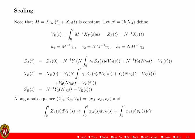
Scaling

Note that M = XAE(t) +XE(t) is constant. Let N = O(XA) define

VE(t) =

∫ t

0

M−1XE(s)ds, ZA(t) = N−1XA(t)

κ1 = M−1γ1, κ2 = NM−1γ2, κ3 = NM−1γ3

ZA(t) = ZA(0)−N−1Y1(N

∫ t

0

γ1ZA(s)dVE(s)) +N−1Y2(Nγ2(t− VE(t)))

XE(t) = XE(0)− Y1(N

∫ t

0

γ1ZA(s)dVE(s)) + Y2(Nγ2(t− VE(t)))

+Y3(Nγ3(t− VE(t)))

ZB(t) = N−1Y3(Nγ3(t− VE(t)))

Along a subsequence (ZA, ZB, VE) ⇒ (xA, xB, vE) and∫ t

0

ZA(s)dVE(s) ⇒∫ t

0

xA(s)dvE(s) =

∫ t

0

xA(s)vE(s)ds


Theorem 1 (Darden [3, 4]) Assume that N →∞, M/N → 0, Mκ1 → γ1, Mκ2/N →γ2, Mκ3/N → γ3, and XA(0)/N → xA(0), and

Then (N−1XA, VE) converges to (xA(t), vE(t)) satisfying

xA(t) = xA(0)−∫ t

0

γ1xA(s)vE(s)ds+

∫ t

0

γ2(1− vE(s))ds (1)

0 = −∫ t

0

γ1xA(s)vE(s)ds+

∫ t

0

(γ2 + γ3)(1− vE(s))ds,

and hence vE(s) = γ2+γ3

γ2+γ3+γ1xA(s)and

xA(t) = − γ1γ3xA(t)

γ2 + γ3 + γ1xA(s).


Quasi-steady state

Assume M is constant κ2 = γ2N/M , κ3 = γ3N/M . Then

f(XE(t))− f(XE(0))−∫ t

0

Nγ1ZA(s)M−1XE(s)(f(XE(s)− 1)− f(XE(s)))ds

−∫ t

0

N(γ2 + γ3)(1−M−1XE(s))(f(XE(s) + 1)− f(XE(s)))ds

Since ZA(s) → xA(s),∫

Cf(xA(s), k)ηs(dk) = 0 becomes

M∑k=0

ηs(k)[(γ1xA(s)M−1k(f(k − 1)− f(k)

+(γ2 + γ3)(1−M−1k)(f(k + 1)− f(k))]

= 0

so ηs is binomial(M, ps), where ps = γ2+γ3

γ2+γ3+γ1xA(s).


Forcing onto a lower dimensional manifold

Assume

F : Rd → Rd

Ξ ⊂ {x ∈ Rd : F (x) = ∞} a submanifold of dimension m < d

∂F (x), x ∈ Ξ, has rank d−m and the nonzero eigenvalues have negative real parts

ψ(t, x) = x+

∫ t

0

F (ψ(s, x))ds,

Υ = {x : Φ(x) ≡ limt→∞ ψ(t, x) exists}

Then, under additional regularity conditions, Φ is C2 and ∂Φ(x)F (x) = 0 in a neigh-borhood of Ξ (Falconer (1983) [5]).


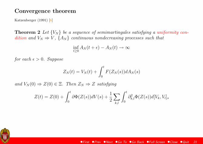
Convergence theorem

Katzenberger (1991) [6]

Theorem 2 Let {VN} be a sequence of semimartingales satisfying a uniformity con-dition and VN ⇒ V , {AN} continuous nondecreasing processes such that

inft≥0

AN(t+ ε)− AN(t) →∞

for each ε > 0. Suppose

ZN(t) = VN(t) +

∫ t

0

F (ZN(s))dAN(s)

and VN(0) ⇒ Z(0) ∈ Ξ. Then ZN ⇒ Z satisfying

Z(t) = Z(0) +

∫ t

0

∂Φ(Z(s))dV (s) +1

2

∑k,l

∫ t

0

∂2k,lΦ(Z(s))d[Vk, Vl]s


Slow time scale limit

Z(t) = Z(0) +∑

k

Yk(

∫ t

0

Nβkλk(Z(s))ds)ΛNζk

= Z(0) +∑

k

Yk(

∫ t

0

Nβkλk(Z(s))ds)(ΛN − Λ0N)ζk

+∑

k

Yk(

∫ t

0

Nβkλk(Z(s))ds)Λ0Nζk

+

∫ t

0

∑k

Nβkλk(Z(s))Λ0Nζkds

Define UN(t) = Z(N−r2t) and assume ζik 6= 0 implies βk − r2 ≤ 2αi and

UN(t) = UN(0) +∑

k

Yk(

∫ t

0

Nβk−r2λk(UN(s))ds)(ΛN − Λ0

N)ζk

+∑

k

Yk(

∫ t

0

Nβk−r2λk(UN(s))ds)Λ0

Nζk

+

∫ t

0

G(UN(s))ds+N r1−r2

∫ t

0

F (UN(s))ds


Negative feedback with dimerization Bratsun, Volfson, Tsimring, and Hasty [2]

A+ A ⇀ A2 A2 ⇀ A+ A

D0 + A2 ⇀ D1 D1 ⇀ D0 + A2

D0 ⇒ D0 + A A ⇀ ∅

The model becomes

θ(t) = θ(0) + Y1(

∫ t

0

κ−1(1− θ(s))ds)− Y2(

∫ t

0

κ1θ(s)X2(s)ds)

X1(t) = X1(0) + Y3(

∫ t−τ

−τ

κ3θ(s)ds)− Y4(

∫ t

0

κ4X1(s)ds)

−2Y5(

∫ t

0

κ2X1(s)(X1(s)− 1)ds) + 2Y6(

∫ t

0

κ−2X2(s)ds)

X2(t) = X2(0) + Y5(

∫ t

0

κ2X1(s)(X1(s)− 1)ds)− Y6(

∫ t

0

κ−2X2(s)ds)

+Y1(

∫ t

0

κ−1(1− θ(s))ds)− Y2(

∫ t

0

κ1θ(s)X2(s)ds).


Scaling

Replace κ−1 byNκ−1, κ−2 byNκ−2, κ3 byNκ3, and (X1(0), X2(0)) by (NZ1(0), NZ2(0)),and divide the three equations by N . Define ZN

1 = N−1XN1 , ZN

2 = N−1XN2

θ(t) = θ(0) + Y1(N

∫ t

0

κ−1(1− θ(s))ds− Y2(

∫ t

0

κ1θ(s)X2(s)ds)

X1(t) = X1(0) + Y3(N

∫ t−τ

−τ

κ3θ(s)ds)− Y4(

∫ t

0

κ4X1(s)ds)

−2Y5(

∫ t

0

κ2X1(s)(X1(s)− 1)ds) + 2Y6(N

∫ t

0

κ−2X2(s)ds)

X2(t) = X2(0) + Y5(

∫ t

0

κ2X1(s)(X1(s)− 1)ds)− Y6(N

∫ t

0

κ−2X2(s)ds)

+Y1(N

∫ t

0

κ−1(1− θ(s))ds)− Y2(

∫ t

0

κ1θ(s)X2(s)ds).


0 ≈∫ t

0

κ−1(1− θN(s))ds)−∫ t

0

κ1θN(s)ZN

2 (s)ds

ZN1 (t) = ZN

1 (0) +N−1Y3(N

∫ t−τ

−τ

κ3θN(s)ds)−N−1Y4(N

∫ t

0

κ4ZN1 (s)ds)

−2N−1Y5(N2

∫ t

0

κ2ZN1 (s)(ZN

1 (s)−N−1)ds) + 2N−1Y6(N2

∫ t

0

κ−2ZN2 (s)ds)

+

∫ t−τ

−τ

κ3θN(s)ds+

∫ t

0

(2κ2 − κ4)ZN1 (s)ds

+N

∫ t

0

2(κ−2ZN2 (s)− κ2Z

N1 (s)2)ds

ZN2 (t) = ZN

2 (0) +N−1Y5(N2

∫ t

0

κ2ZN1 (s)(ZN

1 (s)−N−1)ds)−N−1Y6(N2

∫ t

0

κ−2ZN2 (s)ds)

+N−1Y1(N

∫ t

0

κ−1(1− θN(s))ds)−N−1Y2(N

∫ t

0

κ1θN(s)ZN

2 (s)ds)

−∫ t

0

κ2ZN1 (s)ds+N

∫ t

0

(κ2ZN1 (s)2 − κ−2Z

N2 (s))ds,


Strong drift

F (z1, z2) = (κ−2z2 − κ2z21)

(2−1

)Ξ = {(z1, z2) : z2 =

κ2

κ−2

z21}

Noting that

ZN1 (t) + 2ZN

2 (t) = ZN1 (0) + 2ZN

2 (0)

+N−1Y3(N

∫ t−τ

−τ

κ3θN(s)ds)−N−1Y4(N

∫ t

0

κ4ZN1 (s)ds)

+

∫ t−τ

−τ

κ3θN(s)ds−

∫ t

0

κ4ZN1 (s)ds

+N−1(θ(t)− θ(0))


Limiting equation

Let ε = κ1

κ−1and δ = κ2

κ−2. Then

θ(t) =1

1 + εZ2(t)=

1

1 + εδZ1(t)2

and

Z1(t) + 2δZ1(t)2 = Z1(0) + 2δZ1(0)2 +

∫ t−τ

−τ

κ3

1 + εδZ1(s)2ds−

∫ t

0

κ4Z1(s)ds.


Appendix


Uniformity condition

VN = MN +RN , a semimartingale adapted to {FNt }

Tt(RN), the total variation of RN on [0, t]

[MN ]t, the quadratic variation of MN on [0, t]

Condition 3 a)

{Tt(RN), N = 1, 2, . . .}

is stochastically bounded.

b) There exist stopping times {τ cN} such that

limc→∞

supNP{τ c

N ≤ c} = 0

andsupNE[[MN ]t∧τc

N] <∞


References

[1] Karen Ball, Thomas G. Kurtz, Lea Popovic, and Grzegorz A. Rempala. As-ymptotic analysis of multiscale approximations to reaction networks. Ann. Appl.Probab., 2006. to appear.

[2] Dmitri Bratsun, Dmitri Volfson, Lev S. Tsimring, and Jeff Hasty. Delay-inducedstochastic oscillations in gene regulation. PNAS, 102:14593 – 14598, 2005.

[3] Thomas Darden. A pseudo-steady state approximation for stochastic chemicalkinetics. Rocky Mountain J. Math., 9(1):51–71, 1979. Conference on DeterministicDifferential Equations and Stochastic Processes Models for Biological Systems(San Cristobal, N.M., 1977).

[4] Thomas A. Darden. Enzyme kinetics: stochastic vs. deterministic models. In In-stabilities, bifurcations, and fluctuations in chemical systems (Austin, Tex., 1980),pages 248–272. Univ. Texas Press, Austin, TX, 1982.

[5] K. J. Falconer. Differentiation of the limit mapping in a dynamical system. J.London Math. Soc. (2), 27(2):356–372, 1983.

[6] G. S. Katzenberger. Solutions of a stochastic differential equation forced onto amanifold by a large drift. Ann. Probab., 19(4):1587–1628, 1991.


[7] Thomas G. Kurtz. Averaging for martingale problems and stochastic approxima-tion. In Applied stochastic analysis (New Brunswick, NJ, 1991), volume 177 ofLecture Notes in Control and Inform. Sci., pages 186–209. Springer, Berlin, 1992.


Abstract

Model reduction for chemical reaction networks

Stochastic models of cellular chemical reaction networks typically involve chemicalspecies numbers and reaction rates varying over several orders of magnitude. Anumber of researchers have proposed exploiting the multiscale nature of these modelsto reduce the complexity of the model to be analyzed or simulated. Systematicapproaches to model reduction will be discussed.

Documents

Model reduction for chemical reaction networks