Model Predictive Control Short Course Introductionjbr control Measurement MH Estimate MPC control Forecast t time Reconcile the past Forecast the future sensors y actuators u min u(t)

Model Predictive Control Short Course —Introduction

James B. Rawlings Michael J. Risbeck Nishith R. Patel

Department of Chemical and Biological Engineering

Copyright c© 2017 by James B. Rawlings

Milwaukee, WIAugust 28–29, 2017

JCI – 2017 MPC short course 1 / 70

Outline

1 Overview and Industrial Impact of MPC

2 Dynamic ModelingContinuous time linear differential equationsContinuous time transfer functionsDiscrete time linear difference equationsSoftware for model conversions

3 Predictive Control Compared to Classical PID ControlDifficult dynamicsConstraintsMultivariable interactions

4 Summary


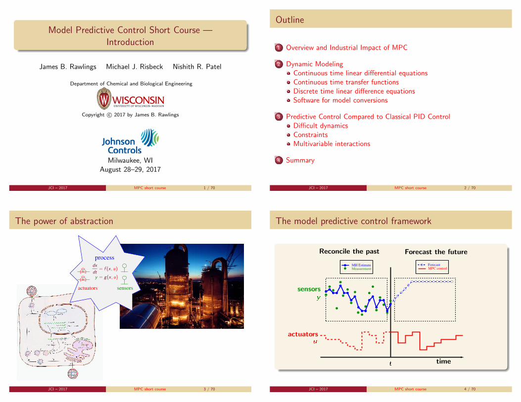
The power of abstraction

process

sensorsactuators

dx

dt= f (x , u)

y = g(x , u)


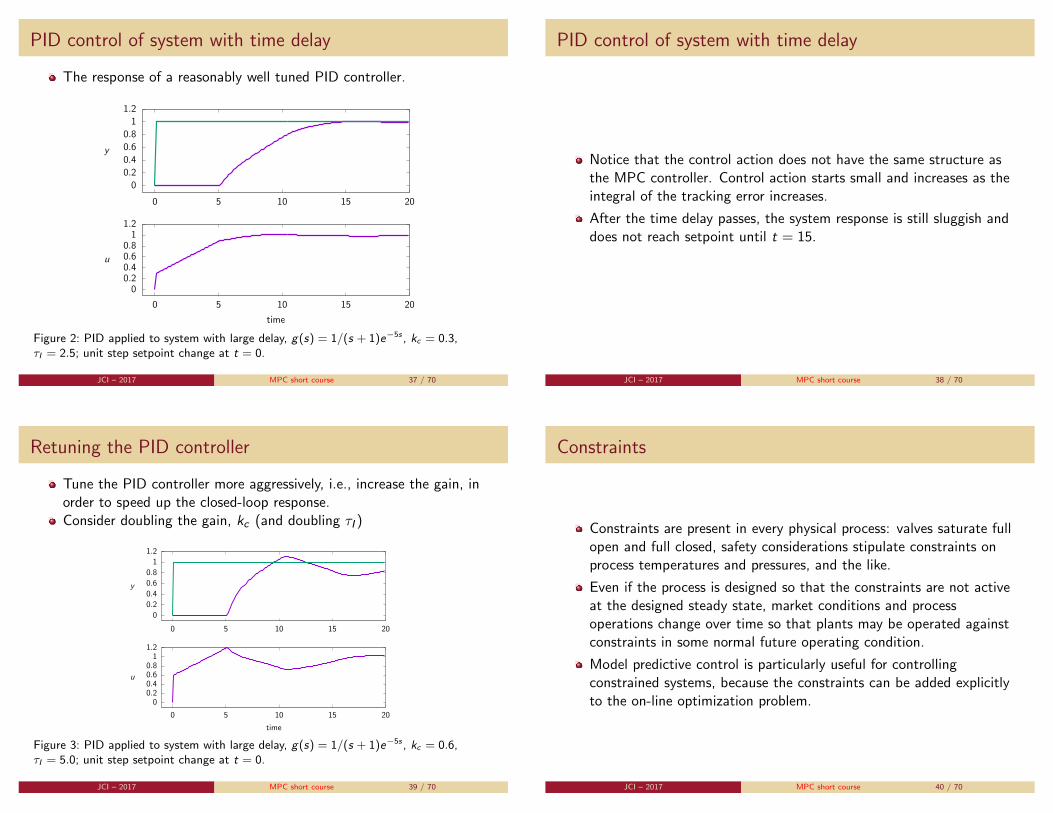
The model predictive control framework

Measurement

MH Estimate

MPC control

Forecast

t time

Reconcile the past Forecast the future

sensorsy

actuatorsu


Predictive control

Measurement

MH Estimate

MPC control

Forecast

t time


sensorsy

actuatorsu

minu(t)

∫ T

0|ysp − g(x , u)|2Q + |usp − u|2R dt

x = f (x , u)

x(0) = x0 (given)

y = g(x , u)JCI – 2017 MPC short course 5 / 70

State estimation

Measurement

MH Estimate

MPC control

Forecast

t time


sensorsy

actuatorsu

minx0,w(t)

∫ 0

−T|y − g(x , u)|2R + |x − f (x , u)|2Q dt

x = f (x , u) + w (process noise)

y = g(x , u) + v (measurement noise)


Industrial impact of the research

Planning and Scheduling

Validation Reconciliation

Model UpdateOptimizationSteady State

Plant

Controller

Two layer structure

Steady-state layerI RTO optimizes steady-state

modelI Optimal setpoints passed to

dynamic layer

Dynamic layerI Controller tracks the setpointsI Linear MPC

(replaces multiloop PID)


Large industrial success story!

Linear MPC and ethylene manufacturing

Number of MPC applications in ethylene: 800 to 1200

Credits 500 to 800 M$/yr (2007)

Achieved primarily by increased on-spec product, decreased energy use

Eastman Chemical experience with MPC

First MPC implemented in 1996

Currently 55-60 MPC applications of varying complexity

30-50 M$/year increased profit due to increased throughput (2008)

Praxair experience with MPC

Praxair currently has more than 150 MPC installations

16 M$/year increased profit (2008)


Impact for 13 ethylene plants (Starks and Arrieta, 2007)

Hydrocarbons AC&O 17

Advanced ControlAdvanced Control& Optimization& Optimization

We’re Doing it For the Money

$0

$10,000,000

$20,000,000

$30,000,000

$40,000,000

$50,000,000

$60,000,000

1Q 2

000

3Q 2

000

1Q 2

001

3Q 2

001

1Q 2

002

3Q 2

002

1Q 2

003

3Q 2

003

1Q 2

004

3Q 2

004

1Q 2

005

3Q 2

005

1Q200

6

3Q200

6

$0

$100,000,000

$200,000,000

$300,000,000

$400,000,000

$500,000,000

$600,000,000

Cumulative Quarterly


Broader industrial impact (Qin and Badgwell, 2003)

Area Aspen Honeywell Adersa PCL MDC TotalTechnology Hi-Spec

Refining 1200 480 280 25 1985

Petrochemicals 450 80 - 20 550

Chemicals 100 20 3 21 144

Pulp and Paper 18 50 - - 68

Air & Gas - 10 - - 10

Utility - 10 - 4 14

Mining/Metallurgy 8 6 7 16 37

Food Processing - - 41 10 51

Polymer 17 - - - 17

Furnaces - - 42 3 45

Aerospace/Defense - - 13 - 13

Automotive - - 7 - 7

Unclassified 40 40 1045 26 450 1601

Total 1833 696 1438 125 450 4542

First App. DMC:1985 PCT:1984 IDCOM:1973 PCL: SMOC:IDCOM-M:1987 RMPCT:1991 HIECON:1986 1984 1988

OPC:1987

Largest App 603x283 225x85 - 31x12 -


Linear differential equations

The linear continuous time model is a set of n first-order linear differentialequations

dx

dt= Ax + Bu

y = Cx + Du (1)

in which

x state n-vectoru manipulated input m-vectory measured output p-vector


SISO and system order

dx

dt= Ax + Bu

y = Cx + Du

For single input, single output (SISO) systems, m = 1 and p = 1, butn, known as the order of the system, may be greater than one (evenfor SISO systems).

The matrix D is often zero. It represents a direct connection from theinput to the output.

If the transfer function discussed below has numerator anddenominator with equal orders, then D 6= 0.


Transfer function model

In the Laplace transform domain, we consider the Laplace transform of theinput u(t), denoted u(s), and the output y(t), denoted y(s). The linearmodel is then the transfer function G (s) relating the input to the output

y(s) = G (s)u(s)

u(s) y(s)G (s)


Converting between ODEs and transfer functions

Example 1 (First-order system)

We are probably already familiar with the first-order system and itstransfer function

G (s) =k

τs + 1

with gain k and time constant τ . Find the corresponding A,B,C ,D in thetime domain differential equations.


First-order system

Solution

First take the relation

y(s) = G (s)u(s) =k

τs + 1u(s)

Rearrange to(τs + 1)y(s) = ku(s)

Invert back to the time domain using L(dy/dt) = sy(s)− y(0) withdeviation variables so x(0) = 0 and y(0) = Cx(0) = 0.

τdy

dt+ y(t) = ku(t)


First-order system

Solution

Identify x(t) = y(t) and have the state space form

dx

dt= −1

τx +

k

τu

dx

dt= Ax + Bu

y = x y = Cx + Du

We see that the differential equation is first order, n = 1, and that

A = −1

τB =

k

τC = 1 D = 0


Higher-order system

Next we work an example where the order of the differential equation ishigher than one.

Example 2 (Second-order system)

Consider the general second-order system corresponding to the transferfunction

G (s) =k

τ2s2 + 2ζτs + 1

with gain k, free time constant τ , and damping coefficient ζ. Find thecorresponding A,B,C ,D in the time domain differential equations.


Second-order system

Solution

We proceed as in the previous example and note that

L(d2ydt2

)= s2y(s)− y ′(0)− sy(0). If the system is initially at steady state,

in deviation variables we have that y(0) = y ′(0) = 0, giving

L(d2ydt2

)= s2y(s), and L

(dydt

)= sy(s). Substituting these into

y(s) = G (s)u(s) and multiplying both sides by the denominator of G (s)gives

τ2 d2y

dt2+ 2ζτ

dy

dt+ y = ku


Second-order system

Solution

Note that to convert this to a set of first-order differential equations, werequire two states. Let x1 = dy/dt and x2 = y . Then the second-orderdifferential equation above can be expressed as

τ2 dx1

dt= −2ζτx1 − x2 + ku

and we add the second differential equation that defines the relationshipbetween x1 and x2

dx2

dt= x1


Second-order system

Solution

We can rearrange these two differential equations into the state spaceform of (1) and write them as a single vector differential equation

d

dt

[x1

x2

]=

[−2ζτ

−1τ2

1 0

] [x1

x2

]+

[kτ2

0

]u

y =[0 1

] [x1

x2

]and we have identified the coefficients

A =

[−2ζτ

−1τ2

1 0

]B =

[kτ2

0

]C =

[0 1

]D = 0


Discrete time linear difference equations

For discrete time systems, we have a sample time, denoted ∆, and weare interested in the state, input and output of the system only at thesample times, t = k∆.

The linear difference equation that represents the behavior at thesample times is given by

x(k + 1) = Adx(k) + Bdu(k)

y(k) = Cdx(k) + Ddu(k) (2)

The following formulas let us convert from the continuous timedifferential equation model to the discrete time model differenceequation model

Ad = eA∆ Bd = A−1(eA∆ − In)B Cd = C Dd = D (3)


Formulas are exact!

Note that if u(t) is a constant between samples (known as azero-order hold), then these formulas are exact and there is noapproximation error such as we would have if we used an Eulermethod to approximate the time derivative in (1).

Note also that if A is singular (one or more of its eigenvalues arezero), A−1 does not exist and the formula for Bd is not defined.

You can obtain Bd from the following relationship that does notrequire A−1

exp

(∆

[A B0 0

])=

[Ad Bd

0 I

]


Convert the first-order system to discrete time

Example 3 (First-order discrete time system)

Convert the first-order continuous time system with time constant τ andgain k to the discrete time system with sample time ∆.

Solution

We have already found the CT state space model is:A = −1/τ , B = k/τ ,C = 1, D = 0. Using the CT to DT conversion formulas (3) gives

Ad = e−∆/τ Bd = k(1− e−∆/τ ) Cd = 1 Dd = 0


Why discrete time models?

Note that the discrete time model is extremely convenient for computersimulation. An example SISO simulation for a second-order system wouldbe:

nts = 100; tfin = nts*delta;

tout = linspace (0, tfin, nts)';

x = zeros(2, nts); y = zeros(1, nts); u = sin(w*tout);

xp = x0;

for k = 1: nts

x(:,k) = xp;

% take measurement

y(k) = Cd*x(:,k);

% update process

xp = Ad*xp + Bd*u(k);

end


Software for model conversions

The conversions between model forms can be carried out conveniently inMatlab or Octave. Useful functions: ss, c2d, and tf.

1 sys = ss(A,B,C,D). Enter a general system using a continuous timestate space model. D is usually zero.

2 dsys = c2d(sys, delta). Convert from a continuous time systemto a discrete time system using sample time delta.

3 Ad = dsys.A, Bd = dsys.B, Cd = dsys.C, Dd = dsys.D

commands extract the state space Ad ,Bd ,Cd ,Dd state spacematrices of the system dsys. Note that the state space model is incontinuous time, (1), or discrete time, (2), depending on whether thesystem dsys is in continuous or discrete time.

4 sys = tf(num, den). Convert from a transfer function model to acontinuous time system. The vectors num and den are the coefficientsof the s polynomial in the numerator and denominator of the transferfunction.


More fine print

Use the help function at the Matlab or Octave prompt to find outmore options for the calling and return arguments for these functions.

Note that you must use expm and not exp in Matlab or Octavewhen exponentiating a matrix in the formula for Ad and Bd .


PID feedback control

Consider the process g and feedback controller gc with output disturbanced and setpoint ysp

gc g

−

y

d

uysp

PID controller takes control action based on current tracking errorand integral (and derivative) of tracking error,

u(t) = kc

(e(t) +

1

τI

∫ t

0e(t ′)dt ′ + τd

d

dte(t)

), e = ysp − y

The control engineer adjusts directly tuning parameters kc , τi , τd .


Predictive control

Pre

sen

t

FuturePast value of

control objective

k + 2k + 1kk − 1

x(t)

t

u(t)

Model.

x(k + 1) = Ax(k) + Bu(k)

y(k) = Cx(k)


Predictive control

Control Objective.

V (x ,u) =N−1∑j=0

`(x(j), u(j)

Constraints.

Du(k) ≤ d , k = 0, 1, . . .N − 1

Hx(k) ≤ h, k = 0, 1, . . .N − 1

Optimization.minu

V (x ,u)

subject to the model and constraints.


Predictive control

Stage cost.

`(x , u) = |ysp − Cx(j)|2Qy+ |u(j)− u(j − 1)|2S

The matrices Qy (p × p) and S (m ×m) are the primary tuningparameters in this approach, and they are usually chosen to bediagonal matrices.

Let e = ysp − Cx . Then each term above is a sum of squares

[e1 e2 . . . ep

]Qy1

Qy2

. . .

Qyp

e1

e2

. . .

ep

=

Qy1e21 + Qy2e

22 + · · ·+ Qype

2p


Predictive control

If you wish to have tight control in certain outputs in the y -vector,you choose the corresponding diagonal elements of Qy large.

If you wish to use only small manipulated variable changes in someactuator, you choose the corresponding diagonal elements of S large.

The loop responds quickly (tight control) when Qy ’s elements arelarge relative to S ’s and responds slowly (loose control) with thereverse tuning.

Qy � S Aggressive control

S � Qy Cautious control

Qyi � Qyj Output (sensor) i is more “important” than output j

Si � Sj Input (actuator) i is more “expensive” than input j


MPC feedback control

The control “law” is the outcome of the optimization. We do not(usually) have a simple closed form like in PID.

The tuning parameters are Qy , S , i.e., the weights on inputs andoutputs

Prediction horizon N is not a tuning parameter. We choose it largeenough to “see” the effects of the inputs on the outputs, but smallenough to have a tractable computation. In favorable cases we canmake N =∞.

We can also use some of the constraint parameters as additionaltuning parameters (rate of change constraints)


Difficult dynamics

Nonminimum phase systems (time delays, right half-plane zeros), andhigh order systems limit the gain that can be used in simple feedbackcontrollers without causing instability or excessive control action.

Predictive control does not suffer from this disadvantage because themodel-based forecasting enables the controller to account for theinherent limitations in the process response.Consider the following first order system with time delay

gc g

−

y

d

uysp

g(s) =k

τs + 1e−θs , k = 1, τ = 1, θ = 5


Time delays

The large time delay compared to time constant severely limits theachievable closed-loop performance of this system.

Consider a unit step change in setpoint, ysp, at t = 0. What wouldwe expect an “ideal” controller to do in this situation?

The physically intuitive answer is to take immediately the controlaction required to drive the system without delay to the desiredsetpoint and then ignore the large tracking error while waiting for thesystem’s time delay to pass; then the output should rise quickly to thesetpoint.

The predictive controller has this inherent time delay compensationbecause the forecast enables it to see that it should wait for the timedelay to pass before taking further control action.


Predictive control of system with time delay

The predictive controller behaves precisely as we expect an idealcontroller to behave. It takes large control action early to achieve thesetpoint and then does nothing further until the time delay passes.

0

0.2

0.4

0.6

0.8

1

1.2

0 5 10 15 20

00.20.40.60.8

11.21.4

0 5 10 15 20

y

u

time

Figure 1: MPC applied to system with large delay, g(s) = 1/(s + 1)e−5s , Q = 1, R = 1,S = 0; unit step setpoint change at t = 0.


PID control

Without a model, the PID controller is blind to the delay and musttake control action based on current tracking error and integral (andderivative) of tracking error,

u(t) = kc

(e(t) +

1

τI

∫ t

0e(t ′)dt ′ + τd

d

dte(t)

), e = ysp − y

Even if we choose kc and τI carefully (we’ll set τd = 0), there is onlyso much that we can expect.


PID control of system with time delay

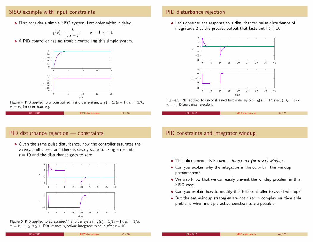
The response of a reasonably well tuned PID controller.

0

0.2

0.4

0.6

0.8

1

1.2

0 5 10 15 20

00.20.40.60.8

11.2

0 5 10 15 20

y

u

time

Figure 2: PID applied to system with large delay, g(s) = 1/(s + 1)e−5s , kc = 0.3,τI = 2.5; unit step setpoint change at t = 0.


PID control of system with time delay

Notice that the control action does not have the same structure asthe MPC controller. Control action starts small and increases as theintegral of the tracking error increases.

After the time delay passes, the system response is still sluggish anddoes not reach setpoint until t = 15.


Retuning the PID controller

Tune the PID controller more aggressively, i.e., increase the gain, inorder to speed up the closed-loop response.Consider doubling the gain, kc (and doubling τI )

0

0.2

0.4

0.6

0.8

1

1.2

0 5 10 15 20

00.20.40.60.8

11.2

0 5 10 15 20

y

u

time

Figure 3: PID applied to system with large delay, g(s) = 1/(s + 1)e−5s , kc = 0.6,τI = 5.0; unit step setpoint change at t = 0.


Constraints

Constraints are present in every physical process: valves saturate fullopen and full closed, safety considerations stipulate constraints onprocess temperatures and pressures, and the like.

Even if the process is designed so that the constraints are not activeat the designed steady state, market conditions and processoperations change over time so that plants may be operated againstconstraints in some normal future operating condition.

Model predictive control is particularly useful for controllingconstrained systems, because the constraints can be added explicitlyto the on-line optimization problem.


SISO example with input constraints

First consider a simple SISO system, first order without delay,

g(s) =k

τs + 1, k = 1, τ = 1

A PID controller has no trouble controlling this simple system.

0

0.2

0.4

0.6

0.8

1

0 5 10 15 20

00.20.40.60.8

11.2

0 5 10 15 20

y

u

time

Figure 4: PID applied to unconstrained first order system, g(s) = 1/(s + 1), kc = 1/k,τI = τ . Setpoint tracking.


PID disturbance rejection

Let’s consider the response to a disturbance: pulse disturbance ofmagnitude 2 at the process output that lasts until t = 10.

−3

−2

−1

0

1

2

0 5 10 15 20 25 30 35 40

−3

−2

−1

0

1

0 5 10 15 20 25 30 35 40

y

u

time

Figure 5: PID applied to unconstrained first order system, g(s) = 1/(s + 1), kc = 1/k,τI = τ . Disturbance rejection.


PID disturbance rejection — constraints

Given the same pulse disturbance, now the controller saturates thevalve at full closed and there is steady-state tracking error untilt = 10 and the disturbance goes to zero

−1

0

1

2

0 5 10 15 20 25 30 35 40

−1

0

0 5 10 15 20 25 30 35 40

y

u

time

Figure 6: PID applied to constrained first order system, g(s) = 1/(s + 1), kc = 1/k,τI = τ , −1 ≤ u ≤ 1. Disturbance rejection; integrator windup after t = 10.


PID constraints and integrator windup

This phenomenon is known as integrator (or reset) windup.

Can you explain why the integrator is the culprit in this windupphenomenon?

We also know that we can easily prevent the windup problem in thisSISO case.

Can you explain how to modify this PID controller to avoid windup?

But the anti-windup strategies are not clear in complex multivariableproblems when multiple active constraints are possible.


Simple PID anti-reset windup

for i = 1: nts

%% take measurement

y(i) = x(i);

%% compute PI control

err = ysp(i) - y(i);

utry = Kc*(err + 1/tauI*interr(i));

%% saturation limits on the valve -ulim <= u <= ulim

if (utry >= ulim) u(i) = ulim;

elseif (utry <= -ulim ) u(i) = -ulim;

else u(i) = utry; end

%% update process and integral (sum) of tracking error

if (i == nts) break end

x(i+1) = A*x(i) + B*u(i);

%% stop integrating if valve is saturated (anti-reset windup)

if ( u(i) == utry )

interr(i+1) = interr(i) + err;

else

interr(i+1) = interr(i);

end

end


PID control with anti-reset windup

−1

0

1

2

0 5 10 15 20 25 30 35 40

−1

0

1

0 5 10 15 20 25 30 35 40

y

u

time

Figure 7: PID applied to constrained first order system with anti-reset windup,g(s) = 1/(s + 1), kc = 1/k, τI = τ , −1 ≤ u ≤ 1. Disturbance rejection; anti-resetwindup after t = 10.


MPC control of constrained system

By contrast, consider the MPC controller behavior

−1

0

1

2

0 5 10 15 20 25 30 35 40

−1

0

1

0 5 10 15 20 25 30 35 40

y

u

time

Figure 8: MPC applied to constrained first-order system, g(s) = 1/(s + 1),Q = 1,R = 1,S = 0,N = 10, −1 ≤ u ≤ 1. Disturbance rejection; no integrator windupafter t = 10.


MPC control of constrained system

Notice that the MPC controller quickly moves the output back tosetpoint at t = 10 after the disturbance goes to zero.

There is no windup problem in an MPC controller.

One does not need to design anti-windup strategies.

The influence of constraints is forecast correctly and handledautomatically by an MPC controller. That is one of the trulyattractive features of MPC for industrial practice.


Multivariable interactions

A significant advantage of MPC comes to light if we examine stronglyinteracting multiinput multioutput (MIMO) systems, which we knowcan cause problems for multiloop SISO PID controllers.

Consider a two-input, two-output process with the following transferfunction (Ogunnaike and Ray, 1994, pp. 757–758).

G (s) =

[2

10s+12

s+1

1s+1

−410s+1

]


Relative gain array (RGA)

The RGA for this process is given by

Λ =

[0.8 0.20.2 0.8

]The RGA indicates that pairing u1–y1, u2–y2 is best considering thesteady-state interactions.

The next figure shows how two SISO PID controllers manage a unitsetpoint change in the first output.


Multiloop PID — RGA pairing

A classic case of two controllers fighting with each other.

−0.20

0.20.40.60.8

11.21.4

0 2 4 6 8 10

−0.50

0.51

1.52

2.5

0 2 4 6 8 10

y1y2

time

u1u2

Figure 9: PID control with steady-state pairing (u1–y1, u2–y2), kc1 = 2, τI1 = 2,kc2 = −2, τI2 = 3; setpoint change in y1.


Multiloop PID — dynamic considerations

G (s) =

[2

10s+12

s+1

1s+1

−410s+1

]

This pairing is not attractive from the dynamic perspective. Themuch slower u1 input is driving y1 (τ11 = 10) when a ten times fasterinput, u2, could have been used (τ12 = 1).

Similarly, the slow input, u2, drives y2 (τ22 = 10) when the first inputis ten times faster (τ21 = 1).

Dynamic considerations would favor switching to the pairing u2–y1,u1–y2.


Multiloop PID — dynamic pairing

−0.20

0.20.40.60.8

11.2

0 2 4 6 8 10

0

1

2

3

4

5

0 2 4 6 8 10

y1y2

time

u1u2

Figure 10: PID control with dynamic pairing (u2–y1, u1–y2), kc1 = 5, τI1 = 2, kc2 = 5,τI2 = 3; setpoint change in y1.


Multiloop PID — pairing summary

For this case, dynamics carry the day and the pairing based on speedof response exhibits better setpoint tracking than the pairing basedon steady-state interactions.

These points are all clear for this example, but they will not be soclear if we start to move the two time constants closer to each otherand the dynamic separation of time scales is not so large.


MPC of multivariable system

Let’s see what happens if we refuse to choose pairings and allow amultivariable MPC controller to use its model to sort things outautomatically.

−0.20

0.20.40.60.8

11.2

0 2 4 6 8 10

0

1

2

3

4

5

0 2 4 6 8 10

y1y2

time

u1u2

Figure 11: Multi-variable MPC control, Qy = I , S = 0. Setpoint change.


MPC of multivariable system

Notice that the performance is essentially deadbeat (i.e. immediate)in moving output y1 to its new setpoint while not disturbing outputy2.

The MPC controller uses its model to forecast exactly what inputtrajectories in both inputs are required to track exactly the setpoint inboth outputs. Interactions are not an issue because the modelforecast accounts for them. (Model error is discussed later.)

Performance is as good or better than the best performance we canachieve using PID with the best tuning constants and the best pairing.

No significant tuning effort for the MPC controller is required toachieve this good nominal performance. We used Q = I , S = 0 forthis deadbeat response.

As we expect, we will have to detune this controller (increase S to useless input) if we want it to accommodate sensor noise, and mismatchbetween the plant and the model.


Effect of tuning parameters: move suppression with S

The effect of increasing the S penalty from 0 to I is shown next

−0.20

0.20.40.60.8

11.2

0 2 4 6 8 10

00.20.40.60.8

11.2

0 2 4 6 8 10

y1y2

time

u1u2

Figure 12: Multi-variable infinite horizon MPC control, Qy = I , S = I . Setpoint change.


Effect of tuning parameters: move suppression with S

The S penalty affects the optimization tradeoff between the outputtracking error and the manipulation of the input.

Notice the output response has slowed down and is no longerdeadbeat, and that the manipulated input is moving less aggressively.


Constraints in multivariable systems

MPC offers further flexibility to shape this tradeoff between outputtracking error and manipulated input. Let us now assume that theinputs are scaled so that valve saturation occurs at u = ±1. Thesecond input violates this constraint in the previous simulation.

A PID controller would clip this signal and saturate the valve.

The MPC controller can be told about these constraints and they canbe treated naturally by the on-line optimization. The results areshown in the next figure.


Constraints in multivariable systems

The output tracking error is not seriously affected while the MPCcontroller deduces what changes to make in the input trajectory toaccount for the valve saturation.

−0.20

0.20.40.60.8

11.2

0 2 4 6 8 10

00.20.40.60.8

11.2

0 2 4 6 8 10

y1y2

time

u1u2

Figure 13: Multi-variable infinite horizon MPC control with input constraints, Qy = I ,S = I , umin = −1, umax = 1. Setpoint change.


Rate of change constraints

Another practically motivated method for shaping the tradeoffbetween tracking and control action is to constrain rather thanpenalize the rate of change of the input.

Practitioners or operators may be comfortable with some rates atwhich the valves may be moved between each controller execution,but may not know how to translate that speed into an appropriate Spenalty without extensive simulation.

In these situations constraining rather than (or in addition to)penalizing the rate of change of the input is simpler to implement.



Assume the initial portion of the input manipulation is unacceptableto the process operators, and they would be more comfortable if uchanged not more than 0.1 in each sample,

−0.1 ≤ ∆u ≤ 0.1

Adding this constraint to the MPC problem produces the results inthe next figure



The input now slows down significantly in the early portion of thesetpoint change.

−0.20

0.20.40.60.8

11.2

0 2 4 6 8 10

00.20.40.60.8

11.2

0 2 4 6 8 10

y1y2

time

u1u2

Figure 14: Multi-variable infinite horizon MPC control with rate of change constraints,Qy = I , S = I , ∆umax = 0.1. Setpoint change.



The rate of change constraint becomes binding in both inputs. Theslower input manipulation in turn affects the speed of response in theoutput.

This kind of simulation allows one to see directly what penalty mustbe paid in the speed of output tracking if one wishes to impose thisrate constraint on the input.


Summary of MPC compared to PID

In this part of the course we have seen that MPC offers significantadvantages compared to PID control in the following situations

1 Difficult dynamics: time delays, right half plane zeros, high ordersystems.

2 Tightly constrained systems: valve saturation, rate of changeconstraints, avoidance of integrator windup.

3 Strongly interacting multivariable systems. No need for pairing, andtrue multivariable control.

Of course MPC does not solve all control problems. The biggestdisadvantage of MPC, or any model-based control system, is thesignificant effort required to obtain a process model and tune thecontroller to handle a variety of plant conditions without humanintervention and constant re-tuning and maintenance.


Summary of MPC compared to PID

Given the successful implementation of MPC in the process industries,however, we can conclude that this modeling effort can pay off inimproved profitability, product quality and safety.

The decision about when to implement MPC versus simple, well-tunedPID controllers requires an assessment of the achievable processimprovements versus the time and expense of the modeling effort.


MPC can be used with nonlinear models

Finally, nothing restricts the ideas of MPC to linear models.Practitioners are now pursuing the implementation of MPC based onnonlinear, fundamental chemical process models.

dx/dt = f (x , u) y = g(x , u)

The on-line optimization becomes significantly more complex, buttoday’s computational capabilities are already up to the task ofimplementation for reasonably sized process units.

The bottlenecks at this point are, again, obtaining nonlinear processmodels from first principles and operating data, and algorithms forreliably solving the nonlinear MPC optimization.


Lab Exercises

Solve the examples in this section and reproduce the figures.Exercise 1.10 (Rawlings and Mayne, 2009)

Example 4

Define a state vector and realize the following models as state spacemodels by hand. One should do a few by hand to understand what theOctave or Matlab calls are doing. Answer the following questions. Whatis the connection between the poles of G and the state space description?For what kinds of G (s) does one obtain a nonzero D matrix? What is theorder and gain of these systems? Is there a connection between order andthe numbers of inputs and outputs?

a G (s) =1

2s + 1

b G (s) =1

(2s + 1)(3s + 1)

c G (s) =2s + 1

3s + 1

d y(k + 1) = y(k) + 2u(k)

e y(k + 1) = a1y(k) + a2y(k − 1) +b1u(k) + b2u(k − 1)


Lab Exercises

Exercise 1.11

Example 5

Find minimal realizations of the state space models you found by hand inExercise 4. Use Octave or Matlab for computing minimal realizations.Were any of your hand realizations nonminimal?


Further reading I

B. A. Ogunnaike and W. H. Ray. Process Dynamics, Modeling, and Control. OxfordUniversity Press, New York, 1994.

S. J. Qin and T. A. Badgwell. A survey of industrial model predictive controltechnology. Control Eng. Pract., 11(7):733–764, 2003.

J. B. Rawlings and D. Q. Mayne. Model Predictive Control: Theory and Design. NobHill Publishing, Madison, WI, 2009. 576 pages, ISBN 978-0-9759377-0-9.

D. M. Starks and E. Arrieta. Maintaining AC&O applications, sustaining the gain. InProceedings of National AIChE Spring Meeting, Houston, Texas, April 2007.


Documents

Model Predictive Control Short Course Introductionjbr control Measurement MH Estimate MPC control Forecast t time Reconcile the past Forecast the future sensors y actuators u min u(t)