Model Predictive Control of Marine Power Plants with Gas

This work is licensed under a Creative Commons Attribution 3.0 License. For more information, see http://creativecommons.org/licenses/by/3.0/.

This article has been accepted for publication in a future issue of this journal, but has not been fully edited. Content may change prior to final publication. Citation information: DOI10.1109/ACCESS.2019.2895163, IEEE Access

Digital Object Identifier

Model Predictive Control of MarinePower Plants with Gas Engines andBatteryTORSTEIN I. BØ1,3, ERLEND VAKTSKJOLD2, EILIF PEDERSEN3, AND OLVE MO41SINTEF Ocean, Otto Nielsens veg 10, 7491 Trondheim, Norway (email: [email protected])2Rolls-Royce Bergen Engines AS, Hordvikneset 125, 5108 Hordvik, Norway, (email:[email protected])3Norwegian University of Science and Technology - NTNU, at Department for Marine Technology, 7491 Trondheim, Norway (email: [email protected])4SINTEF Energy, Sem Sælands vei 11, 7034 Trondheim, Norway (email:[email protected])

The authors of this paper are partly funded by the SFI Smart Maritime, which is mainly supported by the Research Council of Norwaythrough the Centres for Research-based Innovation (SFI) funding scheme, project number 237917. The authors of this paper are funded inpart by the project Optimization of Marine Energy Storage Systems for Desired Lifetime, Energy Saving and Safety, which is primarilysupported by the Research Council of Norway, project number 254766.

ABSTRACT The electric load demand on marine vessels is constantly changing during some operationalmodes, such as in harsh weather or complex operations. Therefore, diesel engines are typically used tohandle these variations. Gas engines reduce the CO2 due to a lower carbon content in LNG compared withdiesel oil. However, they may not be able to handle the load variations of a marine power plant. Thereare multiple other energy sources with strict rate constraints, such as slow speed diesel engines and fuelcells. In such cases, a battery may be used to take care of the variations, while the generator set producesa slowly varying power. In this paper, a common power flow controller for the battery and the generatorset is proposed. It utilizes the rotating inertia in the generator set as energy storage, in addition to a battery.This is done by allowing a small excursion in the speed of the generator set, the speed change will changethe kinetic energy of the generator set and this is used analogous to an energy storage. The controller iscompared with a baseline controller based on virtual inertia and speed-droop. A simulation study is includedto demonstrate the performance of the control methods. The simulation study shows that the gas engine (withstrict constraints) is not able to handle the given load series. Nonetheless, it can be used in combination witha battery to handle the variations. The power plant can handle a measured load series from a offshore vesselwhen either speed-droop control or model predictive control (MPC) is used. However, the study indicatesthat by using MPC, the aging of the batteries and fuel rate variations can be reduced.

INDEX TERMS Energy storage, Gas engine, Predictive control, Power control

I. INTRODUCTIONMarine electric power grids are often subjected to largepower variations. These come from variations in, e.g., en-vironmental loads, thruster demands, hotels demand, craneloads and drilling drives [1]. Traditionally, diesel engines andgas turbines have been used to produce power on marinevessels. One of the reasons for this is that they react fastenough to follow load variations, so that the speed and hencethe electric frequency, does not vary too much.

The Third IMO Greenhouse Gas Study 2014 estimates thatgreenhouse gas emissions from marine vessels will increaseby 50 to 250%, as measured in CO2-equivalents, by 2050for the business as usual scenarios [2]. Yet, it is estimatedthat the peak in net emissions from shipping needs to peak

by 2025 in order to be able to meet the 2-degree goal [3].Alternatives to conventional engines may be used to meetthis target, such as gas engines and fuel cells. Otto-cyclenatural gas engines premix natural gas with air before it iscompressed in the cylinder. If the mixture is too lean it willnot ignite, resulting in methane slip. Conversely, a mixturethat is too rich will autoignite, thus resulting in knocking.Therefore, the engine can only operate in the narrow windowbetween autoignition and misfiring [4]. Load variations makeit harder to control the air/fuel-ratio, as the needed fuel willvary. Hence, Otto-cycle natural gas engines are seldom usedin diesel electric power plants when the power demand highlyvaries. The issue of limited dynamic performance is alsoprominent for engines and alternatives, such as slow speed

VOLUME 4, 2016 1



Bø et al.: Model Predictive Control of Marine Power Plants with Gas Engines and Battery

diesel engines and proton exchange membrane fuel cells [5].By combining an Otto-cycle natural gas engine and a battery,the load variations can be handled by the battery, whereas themean power can be generated by the engines.

In terms of lithium ion batteries, energy storage has al-ready been used in some marine applications. This includesplatform support vessels (Edda Ferd [6], Viking Lady [7]),ferries (Prinsesse Benedikte [8], Ampere [9], Tycho Braheand Tycho Aurora [10]), tugboats (RT Adriaan [11]), high-speed passenger feries (BB Green [12]) and sightseeingvessels (Vision of the Fjords [13]). The battery packs havemany use cases such as: spinning reserve, peak shaving,power smoothing, enhanced dynamic performance, strategicloading and zero emission operation [14], [15].

Variable speed engines have also been suggested for ma-rine power plants. This can be achieved with a direct current(dc) grid, implemented by multiple vendors [9]. With a directcurrent grid, a rectifier is placed between the synchronousgenerator and the dc grid. An alternative approach is the"Dynamic AC" concept by ABB [16]. With this concept, themain grid runs with variable frequency ac. Frequency con-verters are then placed between the grid and each consumeror distribution grid. Both systems allow the generator setsto run at any desired speed, typically from a speed of 70–105%. This provides an opportunity to lower the speed whenthe power demand is low, as this reduces the specific fuelconsumption of the engines. Note that a fixed frequency acgrid is used in this article, which allows the frequency to varyfrom 5 to 10%.

In this paper, model predictive control (MPC) is used tocontrol the power plant. With MPC, a model of the plantis used to optimize the performance of the plant. The MPCpredicts the future state and control trajectory. These tra-jectories are optimized to minimize the value of the costfunction. Because model errors and disturbances may occur,the control optimization problem is solved again at every timestep of the controller.

The power demand must be divided between multipledevices when a hybrid power plant is used. This task ofsplitting the power production between an engine and energystorage is not trivial. MPC is one of the already suggestedmethods for this task. A combination of battery and ultraca-pacitors for load smoothing is presented in [17]. The articlepresents two controllers: One combined control by modelpredictive control (MPC) of the battery and ultracapacitors.The second controller separates the power variations by alow pass filter and uses two MPCs to individually controlthe battery and ultracapacitors. An MPC that minimizes thepower tracking error or the energy storage losses is presentedin [18]. The cost function allows the user to weight the rela-tive importance of energy storage losses and power trackingerrors. The controller is demonstrated for a hybrid energystorage consisting of a battery and flywheel and a batteryand ultracapacitors. The use of capacitor bank for powersmoothing is presented in [19]. The controller uses filtering,in addition to the power available signal, to help regulate the

charging and discharging of the capacitor bank. In [20], aband-pass filter is used to filter out the load variations, whichshould be canceled. The filter is tuned by an MPC, suchthat the temperature of the batteries is controlled below anupper limit. In [21], a two-level MPC is used to optimize theperformance of a seagoing vessel. An outer MPC is used tooptimize the reference trajectory of the propeller shaft speed.This reference is given to an inner MPC, which optimizes thepower plant by controlling the power split between the dieselengine, battery and capacitor pack.

The power split problem also arise in other fields. Inan island grid, the problem has been studied for a plantwith photo voltaic-, wind-, diesel- and battery-systems [22].The paper presents the control of frequency and voltageby PI- and fuzzy logic controllers. In [23], particle swarmoptimization is used to tune PI controllers for frequencyregulation of a similar grid. For serial hybrid electric vehicles,heuristics are presented in [24] for the power split between aDC source and battery. The use and control of hybrid energystorage with an ultracapacitor is studied in [25]. Dynamicprogramming is used to optimize the power split betweenan internal combustion engine and a battery pack in a serieshybrid electric vehicle [26].

This paper presents a combined controller for generatorsets and a battery. The purpose of the controller is to utilizethe inherent energy storage of the rotating inertia of thegenerator sets, such that stricter rate constraints can be usedon the gas engines, while the use of the battery is reduced.The generator sets have a jump-rate constraint; this is a con-straint often used by engine suppliers to keep air/fuel withinthe operational window. Most port fuel injection engines arecapable of a small-scale (±5–10%) instant fuel change withno significant fuel/emission cost. Model predictive control isused in this article to control the generator set and battery.Two weight configurations are shown, one which allows avarying frequency (frequency barrier mode) and one with astiff frequency. A varying frequency reduces the use of thebattery by using the rotating inertia of the generator set asan additional energy storage, whereas a stiff frequency canbe needed when new generator sets are synchronizing to thegrid.

The structure of the paper is as follows: Models of thepower plant are presented in the next section. The proposedcontroller and a baseline controller are presented in Sec-tion III. The simulated results are shown in Sections IV anddiscussed in Section V. Conclusions are then drawn in thelast section.

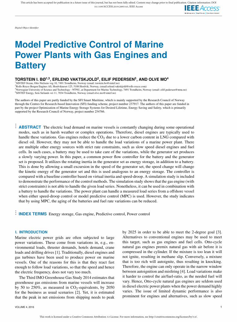
II. MODELSTwo models of the plant are used in this article, the pro-cess plant model, used for simulation and the control plantmodel, used in the controller. The process plant model hasthe highest fidelity and should capture the most importantdynamics of the plant. The control plant model is a simplifiedmodel, such that it can be used internally in the controller. Anoverview of the plant is shown in Figure 1.

2 VOLUME 4, 2016




MPC

G G

u1 u2 pES

Loads

FIGURE 1. Overview of the power plant including the MPC. The MPCcommands the fuel rate to the two gas engines, in addition to a chargingdemand to the battery system. A DC/AC converter is used to control the powerbetween the battery and the main grid, where the two synchronous generatorsof the gas engines are connected. The power demand is given by a timeseries.

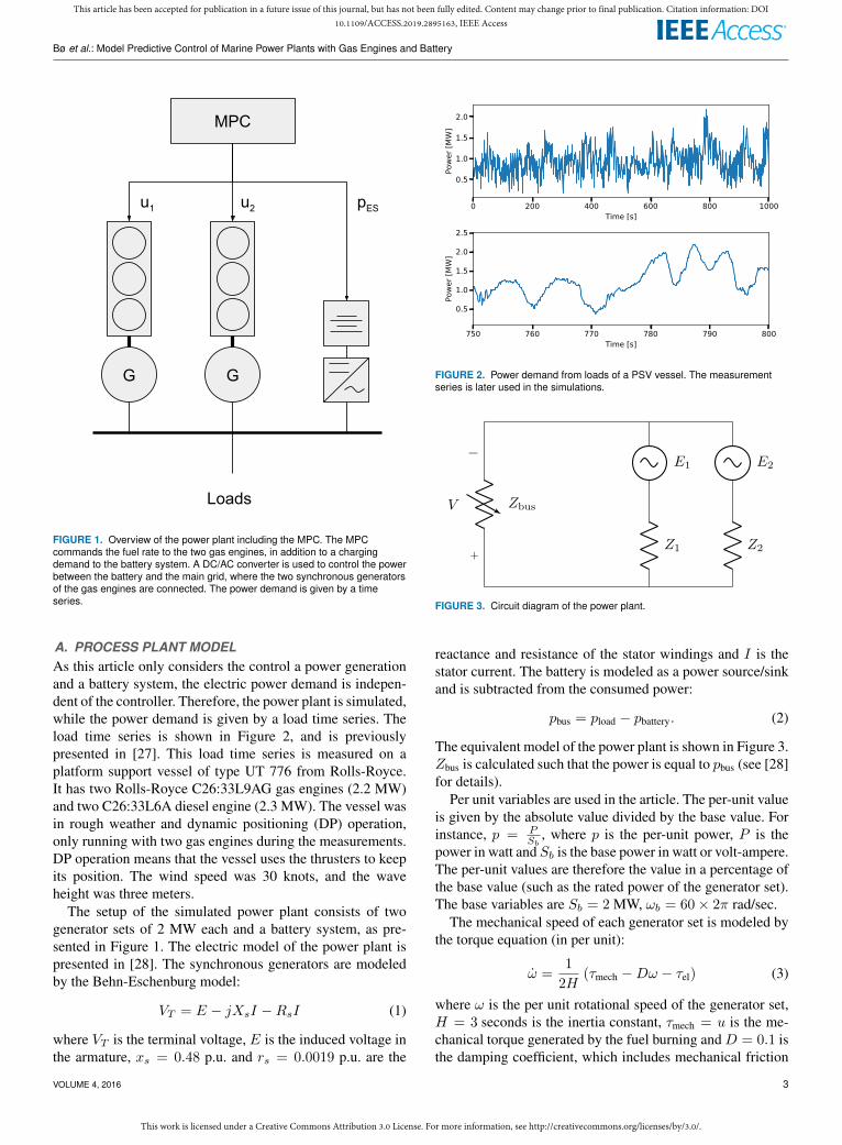
A. PROCESS PLANT MODELAs this article only considers the control a power generationand a battery system, the electric power demand is indepen-dent of the controller. Therefore, the power plant is simulated,while the power demand is given by a load time series. Theload time series is shown in Figure 2, and is previouslypresented in [27]. This load time series is measured on aplatform support vessel of type UT 776 from Rolls-Royce.It has two Rolls-Royce C26:33L9AG gas engines (2.2 MW)and two C26:33L6A diesel engine (2.3 MW). The vessel wasin rough weather and dynamic positioning (DP) operation,only running with two gas engines during the measurements.DP operation means that the vessel uses the thrusters to keepits position. The wind speed was 30 knots, and the waveheight was three meters.

The setup of the simulated power plant consists of twogenerator sets of 2 MW each and a battery system, as pre-sented in Figure 1. The electric model of the power plant ispresented in [28]. The synchronous generators are modeledby the Behn-Eschenburg model:

VT = E − jXsI −RsI (1)

where VT is the terminal voltage, E is the induced voltage inthe armature, xs = 0.48 p.u. and rs = 0.0019 p.u. are the

0 200 400 600 800 1000Time [s]

0.5

1.0

1.5

2.0

Powe

r [M

W]

750 760 770 780 790 800Time [s]

0.5

1.0

1.5

2.0

2.5

Powe

r [M

W]

FIGURE 2. Power demand from loads of a PSV vessel. The measurementseries is later used in the simulations.

Zbus

+

−

V

Z1

E1

Z2

E2

FIGURE 3. Circuit diagram of the power plant.

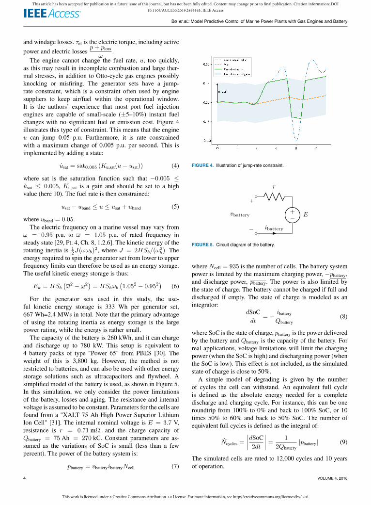
reactance and resistance of the stator windings and I is thestator current. The battery is modeled as a power source/sinkand is subtracted from the consumed power:

pbus = pload − pbattery. (2)

The equivalent model of the power plant is shown in Figure 3.Zbus is calculated such that the power is equal to pbus (see [28]for details).

Per unit variables are used in the article. The per-unit valueis given by the absolute value divided by the base value. Forinstance, p = P

Sb, where p is the per-unit power, P is the

power in watt and Sb is the base power in watt or volt-ampere.The per-unit values are therefore the value in a percentage ofthe base value (such as the rated power of the generator set).The base variables are Sb = 2 MW, ωb = 60× 2π rad/sec.

The mechanical speed of each generator set is modeled bythe torque equation (in per unit):

ω =1

2H(τmech −Dω − τel) (3)

where ω is the per unit rotational speed of the generator set,H = 3 seconds is the inertia constant, τmech = u is the me-chanical torque generated by the fuel burning and D = 0.1 isthe damping coefficient, which includes mechanical friction

VOLUME 4, 2016 3




and windage losses. τel is the electric torque, including activepower and electric losses

p+ ploss

ω.

The engine cannot change the fuel rate, u, too quickly,as this may result in incomplete combustion and large ther-mal stresses, in addition to Otto-cycle gas engines possiblyknocking or misfiring. The generator sets have a jump-rate constraint, which is a constraint often used by enginesuppliers to keep air/fuel within the operational window.It is the authors’ experience that most port fuel injectionengines are capable of small-scale (±5–10%) instant fuelchanges with no significant fuel or emission cost. Figure 4illustrates this type of constraint. This means that the engineu can jump 0.05 p.u. Furthermore, it is rate constrainedwith a maximum change of 0.005 p.u. per second. This isimplemented by adding a state:

usat = sat0.005 (Ku,sat(u− usat)) (4)

where sat is the saturation function such that −0.005 ≤usat ≤ 0.005, Ku,sat is a gain and should be set to a highvalue (here 10). The fuel rate is then constrained:

usat − uband ≤ u ≤ usat + uband (5)

where uband = 0.05.The electric frequency on a marine vessel may vary from

ω = 0.95 p.u. to ω = 1.05 p.u. of rated frequency insteady state [29, Pt. 4, Ch. 8, 1.2.6]. The kinetic energy of therotating inertia is 1

2J(ωωb)2, where J = 2HSb/(ω

2b ). The

energy required to spin the generator set from lower to upperfrequency limits can therefore be used as an energy storage.The useful kinetic energy storage is thus:

Ek = HSb

(ω2 − ω2

)= HSbωb

(1.052 − 0.952

)(6)

For the generator sets used in this study, the use-ful kinetic energy storage is 333 Wh per generator set,667 Wh=2.4 MWs in total. Note that the primary advantageof using the rotating inertia as energy storage is the largepower rating, while the energy is rather small.

The capacity of the battery is 260 kWh, and it can chargeand discharge up to 780 kW. This setup is equivalent to4 battery packs of type "Power 65" from PBES [30]. Theweight of this is 3,800 kg. However, the method is notrestricted to batteries, and can also be used with other energystorage solutions such as ultracapacitors and flywheel. Asimplified model of the battery is used, as shown in Figure 5.In this simulation, we only consider the power limitationsof the battery, losses and aging. The resistance and internalvoltage is assumed to be constant. Parameters for the cells arefound from a "XALT 75 Ah High Power Superior LithiumIon Cell" [31]. The internal nominal voltage is E = 3.7 V,resistance is r = 0.71 mΩ, and the charge capacity ofQbattery = 75 Ah = 270 kC. Constant parameters are as-sumed as the variations of SoC is small (less than a fewpercent). The power of the battery system is:

pbattery = vbatteryibatteryNcell (7)

FIGURE 4. Illustration of jump-rate constraint.

ibattery

−+ E

r

+

−

vbattery

FIGURE 5. Circuit diagram of the battery.

where Ncell = 935 is the number of cells. The battery systempower is limited by the maximum charging power, −pbattery,and discharge power, pbattery. The power is also limited bythe state of charge. The battery cannot be charged if full anddischarged if empty. The state of charge is modeled as anintegrator:

dSoCdt

= − ibattery

Qbattery(8)

where SoC is the state of charge, pbattery is the power deliveredby the battery and Qbattery is the capacity of the battery. Forreal applications, voltage limitations will limit the chargingpower (when the SoC is high) and dischargning power (whenthe SoC is low). This effect is not included, as the simulatedstate of charge is close to 50%.

A simple model of degrading is given by the numberof cycles the cell can withstand. An equivalent full cycleis defined as the absolute energy needed for a completedischarge and charging cycle. For instance, this can be oneroundtrip from 100% to 0% and back to 100% SoC, or 10times 50% to 60% and back to 50% SoC. The number ofequivalent full cycles is defined as the integral of:

Ncycles =

∣∣∣∣dSoC2dt

∣∣∣∣ =1

2Qbattery|pbattery| (9)

The simulated cells are rated to 12,000 cycles and 10 yearsof operation.

4 VOLUME 4, 2016




B. CONTROL PLANT MODELThe control plant model is based on [32], and is used in theMPC. The model assumes that the speeds of the generatorsets are close to equal. This happens due to synchronizationtorque, which keeps the generators at the same frequency.Moreover, damping in the generators (e.g. damping windingsand friction) will damp oscillation between the generator sets.The frequency dynamic is derived from the energy balance:∑

i

2Sb,iHiωi =∑i

Sb,i [τmech,i −Diωi − τel,i] (10)

where subscript i indicates generator set i, and Sb is the basepower of the generator set (it converts the per unit power topower).

It is assumed that the frequency is equal for all generators(i.e., ω = ωi). In addition, the stator resistance is small. Itis therefore assumed that electric losses in the generator aresmall. This gives: pbus ≈

∑i τel,iωi. The total power on the

generators is the difference between the power of the loadsand the delivered battery power, pbus = pload − pbattery. Thisgives:(∑

i

2Sb,iHi

)ω =

(∑i

Sb,iτmech,i

)−(∑

i

Sb,iDi

)ω

− pload − pbattery

ω(11)

The resistance is neglected in the battery model, so thestate of charge is therefore:

dSoCdt

= − pbattery

QbatteryENcell(12)

III. CONTROLLERSA. MODEL PREDICTIVE CONTROLLERA centralized model predictive control (MPC) is used to con-trol both the generator sets and the battery. Model predictivecontrol is a control method based on repeated optimization,with the basis being a cost function and a model of the plant.The MPC predicts a state trajectory for the plant. The costfunction puts a cost to the states and control trajectory, suchas deviation of the states from the reference value and thecost of using the control inputs. The MPC then optimizes thepredicted trajectories so that the cost function is minimized;this optimization may hence be constrained by state andcontrol constraints. The MPC will then implement the firsttime step in the optimized control trajectory. At the next timeinstant the optimization problem is solved again with newstate measurements, and the newly optimized control input isused. This reoptimization is done at every time step.

An overview of the topology of the plant is shown inFigure 1. The MPC commands the fuel rate to the generatorsets, uMPC and power set points to the battery, pbattery. The fuelrate, uMPC, is then controlled by the engine, it is assumed thatthe engine produce a mechanical torque proportional to uMPC.The battery is assumed to be controlled by a power converter,which is able to control the battery power. The task of the

MPC is to keep the frequency within a certain band withoutviolating the constraints of the power plant.

The electric frequency on a marine vessel may vary from95% to 105% of the rated frequency in steady state [29,Pt.4,Ch.8,1.2.6]. A soft constraint is therefore used to avoidlarger frequency variations:

ωouter ≤ ω + sω,outer ≤ ωouter (13)

where underbars and overbars indicate lower and upper con-straint limits, and s denotes a slack variable. Soft constraintsare used to avoid that the optimization problem becomesinfeasible when it is not possible to satisfy the constraints. Asmall safety margin is added to the constraints, which givesωouter = 0.96 pu and ωouter = 1.04 p.u..

In addition, safety functions may reduce the power demandwhen smaller frequency variations occur [33]. Therefore, anadditional inner soft frequency constraint is added:

ωinner ≤ ω + sω,inner ≤ ωinner (14)

This makes it possible to use the inertia of the engines forenergy storage. The frequency may then travel freely betweenωinner = 0.97 p.u. and ωinner = 1.03 p.u. Figure 6 illustratesthe frequency cost function.

The battery is constrained by a maximum power and stateof charge (SoC) range:

pbattery ≤ pbattery ≤ pbattery (15)

SoC ≤ SoC ≤ SoC (16)

A cost on deviation from the reference state of charge, SoCrefis included. This is done to make sure that the battery is notdischarged or charged over the long term, whereas the SoC atthe end of the simulation is equal or close to the SoC at thebeginning of the simulation.

The generator set is jump rate constrained. Note that (4) isnot smooth due to the saturation function, which may causenumerical problems for the solver. The saturation function istherefore approximated by the hyperbolic tangent function:

sata(x) ≈ a tanh(xa

)= a

[2

1 + e−2xa

− 1

](17)

This gives

usat = uusat,max

2

1 + exp(

−2Ku,sat(u−usat)uusat,max

) − 1

(18)

where uusat,max = 0.005. Furthermore, the constraint on thefuel rate is:

usat − uband ≤ u ≤ usat + uband (19)

The generator set limits must also be enforced:

u ≤ u ≤ u (20)

These are hard constraints, since they are the physical limitsof the generator. The controller optimizes the time derivative

VOLUME 4, 2016 5




ωoute

r

ωin

ner

ωre

f

ωin

ner

ωoute

r

Frequency

Cost

Frequency cost with frequency barrier mode

ωoute

r

ωin

ner

ωre

f

ωin

ner

ωoute

r

Frequency

Cost

Frequency cost with stiff frequency mode

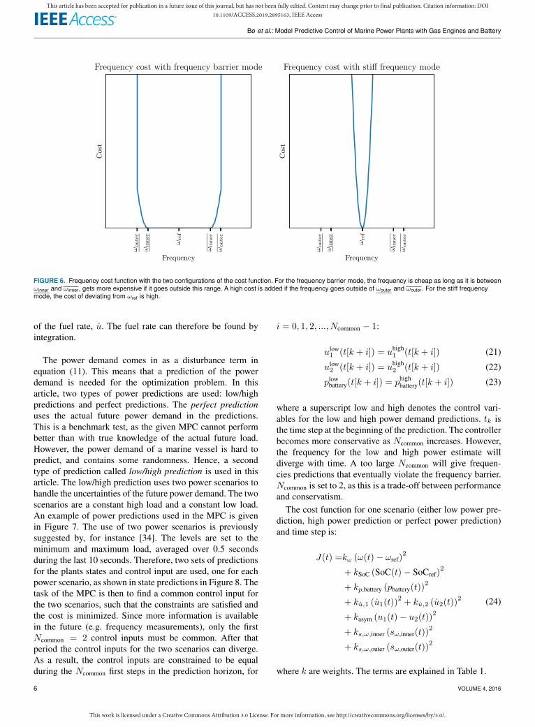
FIGURE 6. Frequency cost function with the two configurations of the cost function. For the frequency barrier mode, the frequency is cheap as long as it is betweenωinner and ωinner, gets more expensive if it goes outside this range. A high cost is added if the frequency goes outside of ωouter and ωouter. For the stiff frequencymode, the cost of deviating from ωref is high.

of the fuel rate, u. The fuel rate can therefore be found byintegration.

The power demand comes in as a disturbance term inequation (11). This means that a prediction of the powerdemand is needed for the optimization problem. In thisarticle, two types of power predictions are used: low/highpredictions and perfect predictions. The perfect predictionuses the actual future power demand in the predictions.This is a benchmark test, as the given MPC cannot performbetter than with true knowledge of the actual future load.However, the power demand of a marine vessel is hard topredict, and contains some randomness. Hence, a secondtype of prediction called low/high prediction is used in thisarticle. The low/high prediction uses two power scenarios tohandle the uncertainties of the future power demand. The twoscenarios are a constant high load and a constant low load.An example of power predictions used in the MPC is givenin Figure 7. The use of two power scenarios is previouslysuggested by, for instance [34]. The levels are set to theminimum and maximum load, averaged over 0.5 secondsduring the last 10 seconds. Therefore, two sets of predictionsfor the plants states and control input are used, one for eachpower scenario, as shown in state predictions in Figure 8. Thetask of the MPC is then to find a common control input forthe two scenarios, such that the constraints are satisfied andthe cost is minimized. Since more information is availablein the future (e.g. frequency measurements), only the firstNcommon = 2 control inputs must be common. After thatperiod the control inputs for the two scenarios can diverge.As a result, the control inputs are constrained to be equalduring the Ncommon first steps in the prediction horizon, for

i = 0, 1, 2, ..., Ncommon − 1:

ulow1 (t[k + i]) = uhigh

1 (t[k + i]) (21)

ulow2 (t[k + i]) = uhigh

2 (t[k + i]) (22)

plowbattery(t[k + i]) = phigh

battery(t[k + i]) (23)

where a superscript low and high denotes the control vari-ables for the low and high power demand predictions. tk isthe time step at the beginning of the prediction. The controllerbecomes more conservative as Ncommon increases. However,the frequency for the low and high power estimate willdiverge with time. A too large Ncommon will give frequen-cies predictions that eventually violate the frequency barrier.Ncommon is set to 2, as this is a trade-off between performanceand conservatism.

The cost function for one scenario (either low power pre-diction, high power prediction or perfect power prediction)and time step is:

J(t) =kω (ω(t)− ωref)2

+ kSoC (SoC(t)− SoCref)2

+ kp,battery (pbattery(t))2

+ ku,1 (u1(t))2

+ ku,2 (u2(t))2

+ kasym (u1(t)− u2(t))2

+ ks,ω,inner (sω,inner(t))2

+ ks,ω,outer (sω,outer(t))2

(24)

where k are weights. The terms are explained in Table 1.

6 VOLUME 4, 2016




5 10 15 20 25Time [s]

0.5

0.6

0.7

0.8

0.9

1.0

Powe

r [M

W]

LoadAveraged load

Minimum loadMaximum load

Low load predictionHigh load prediction

FIGURE 7. Prediction of the future power demand. A high and a low estimateis used. This is done by calculating the average load during one sample period(0.5 seconds); then the minimum and maximum load for the previous 10seconds is found. This is set as the predicted low and high load.

A terminal cost is also included:

JN (t) =kω,N (ω(t)− ωref)2

+ kSoC,N (SoC(t)− SoCref)2 (25)

The total cost function is:

Φ =N−1∑i=0

[J low (t[k + i]) + Jhigh (t[k + i])

]+ J low

N (tk+N ) + JhighN (tk+N ) (26)

The optimization problem is:

minulow,plow

battery,uhigh,phigh

battery

Φ

such that (11− 23)

ωlow(tk) = ωhigh(tk) = ωi

SoClow(tk) = SoChigh(tk) = SoCi

ulow1 (tk) = uhigh

1 (tk) = ui1

ulow2 (tk) = uhigh

2 (tk) = ui2

(27)

where N is the length of the prediction horizon, andωi, soci, um1 , and ui2 are initial values at the current time step.

Two different configurations of weights are used in thecost function. The first configuration, the frequency barriermode, uses a low cost on frequency variations, but large onthe use of the battery. This configuration can be used to avoidunnecessary use, and hence cycling, of the battery. The sec-ond configuration, the stiff frequency mode, uses a high coston frequency variations, but a low cost on using the battery.This can be used when a constant frequency is needed, forexample for an easier synchronization of additional generatorsets.

As is normally done with MPC, the first control input in theprediction horizon from (27) is used. At the following timestep, equation (27) is reoptimized with new initial conditions.

The MPC is implemented in ACADO using the codeexport functionality [35]. The prediction horizon, N, is set to20 samples, with a sampling time of 0.5 seconds. The opti-mization problem consists of 200 optimization variables and209 constraints. ACADO solves the optimization problem asa sequential quadratic problem. The computational time isapproximately 15 to 60 ms, and with an Intel Xeon CPUE4-1245 3.5 GHz processor, the computational time dependson the number of needed SQP iterations. The controller istherefore able to run in real-time.

B. BASELINE CONTROLLER: SPEED-DROOP ANDVIRTUAL SYNCHRONOUS MACHINEA baseline controller is used to compare the response of theMPC with the response from commonly used speed-droopcontroller for the generator set and a power smoothing con-troller for the battery based on virtual inertia and frequencyrecovery.

1) Speed-droop ControlA speed-droop controller calculates a set-point for the fre-quency based on the measured power of the generator:

ωset = ωno-load(1− pDroop) (28)

where ωno-load = 1.01 is the no-load frequency and Droop=0.02 is the speed-droop gain. Note that in many marine powerplants compensated droop is used. This outer controller ad-justs the no-load frequency, such that the frequency is keptcloser to the nominal frequency. This is not included in thecurrent implementation, but can easily be included.

The reference frequency is given to a PID controller, whichsets the fuel rate:

u = KP (ωset − ω) +KI

∫(ωset − ω)dt+KD

ˆω (29)

where KP , KI , KD are control gains given in Table 2.ˆω is an estimate of the time derivative of the generatorsets frequency, and it is calculated by dirty derivatives (alsoknown as bandlimited derivatives).

2) Battery ControllerA virtual generator is used, in addition to a frequency re-covery method to control the battery. To avoid frequencyvariations, the battery is controlled to act as a free spinningsynchronous generator with no losses. This is done by mod-eling a virtual generator, using the same models as for thegenerator sets, i.e., equation (1). The calculated power of thevirtual generator is delivered by the battery. When the electricfrequency of the grid decreases the load on the modeledgenerator will increase, as the load angle of the modeledgenerator increases. This modeled load is then commanded tothe battery system. This modeled rotating mass will decreaseits speed as the electric torque is applied on the shaft, whilethe opposite occurs when the frequency increases. Virtualgenerator control holds the proven properties of synchronous

VOLUME 4, 2016 7




TAB

LE1.

Weights

incostfunction.

Costw

eightFrequency

barrierm

odeStifffrequency

mode

kω

(ω−ω

ref )2

Costofdeviation

fromthe

electricfrequency

reference10−4

104

kSoC

(SoC−

SoCref )

2C

ostofdeviationfrom

thestate

ofchargereference

104

10−1

kp,battery

p2battery

Costofusing

powerfrom

thebattery

104

10−1

ku,1

u21

Costofchanging

thefuelrate

positionofengine

110

7100

ku,2

u22

Costofchanging

thefuelrate

positionofengine

210

7100

kasym

(u1 −

u2 )

2C

ostofasymm

etricfuelrate

positionon

engine10

10ks,ω

,inners2ω

,innerC

ostoffrequencydeviation

outsideofω

inner andω

inner107

104

ks,ω

,outers2ω

,outerC

ostoffrequencydeviation

outsideofω

outer andω

outer10

10

106

kω,N

(ω−ω

ref )2

Costofdeviation

fromthe

electricfrequency

referenceatend

ofthe

predictionhorizon

108

108

kSoC

,N(SoC

−SoC

ref )2

Costofdeviation

fromthe

stateofcharge

atendofthe

predictionhorizon

107

103

8 VOLUME 4, 2016




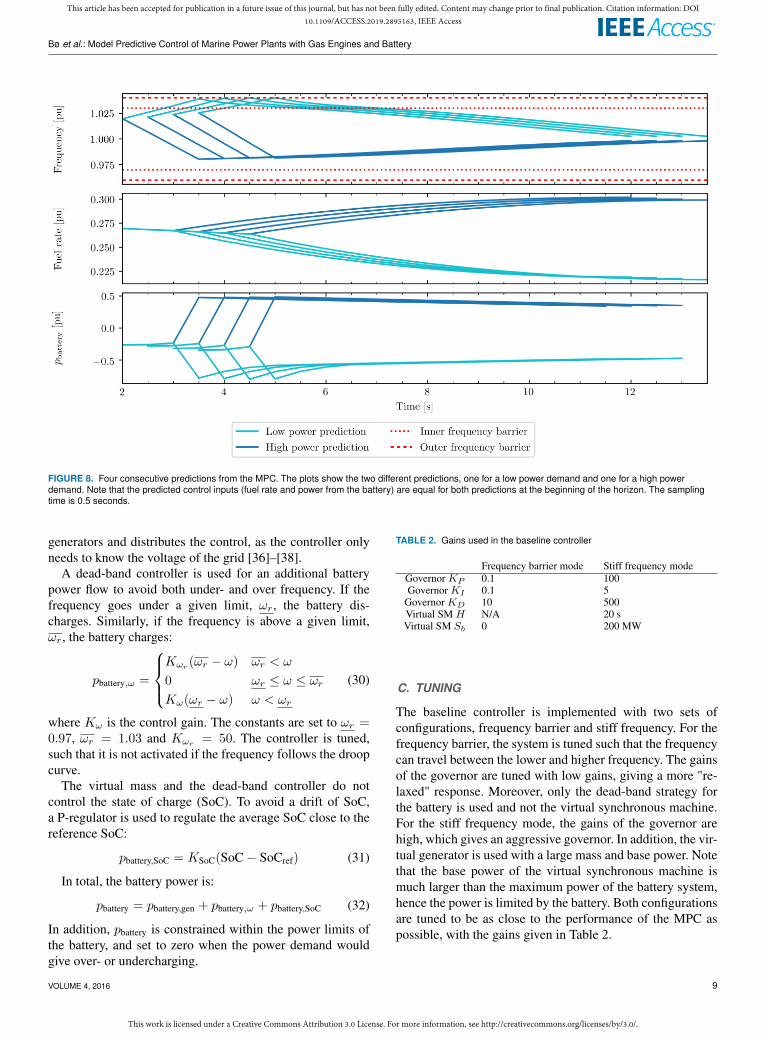
FIGURE 8. Four consecutive predictions from the MPC. The plots show the two different predictions, one for a low power demand and one for a high powerdemand. Note that the predicted control inputs (fuel rate and power from the battery) are equal for both predictions at the beginning of the horizon. The samplingtime is 0.5 seconds.

generators and distributes the control, as the controller onlyneeds to know the voltage of the grid [36]–[38].

A dead-band controller is used for an additional batterypower flow to avoid both under- and over frequency. If thefrequency goes under a given limit, ωr, the battery dis-charges. Similarly, if the frequency is above a given limit,ωr, the battery charges:

pbattery,ω =

Kωr (ωr − ω) ωr < ω

0 ωr ≤ ω ≤ ωr

Kω(ωr − ω) ω < ωr

(30)

where Kω is the control gain. The constants are set to ωr =0.97, ωr = 1.03 and Kωr = 50. The controller is tuned,such that it is not activated if the frequency follows the droopcurve.

The virtual mass and the dead-band controller do notcontrol the state of charge (SoC). To avoid a drift of SoC,a P-regulator is used to regulate the average SoC close to thereference SoC:

pbattery,SoC = KSoC(SoC− SoCref) (31)

In total, the battery power is:

pbattery = pbattery,gen + pbattery,ω + pbattery,SoC (32)

In addition, pbattery is constrained within the power limits ofthe battery, and set to zero when the power demand wouldgive over- or undercharging.

TABLE 2. Gains used in the baseline controller

Frequency barrier mode Stiff frequency modeGovernor KP 0.1 100Governor KI 0.1 5

Governor KD 10 500Virtual SM H N/A 20 sVirtual SM Sb 0 200 MW

C. TUNING

The baseline controller is implemented with two sets ofconfigurations, frequency barrier and stiff frequency. For thefrequency barrier, the system is tuned such that the frequencycan travel between the lower and higher frequency. The gainsof the governor are tuned with low gains, giving a more "re-laxed" response. Moreover, only the dead-band strategy forthe battery is used and not the virtual synchronous machine.For the stiff frequency mode, the gains of the governor arehigh, which gives an aggressive governor. In addition, the vir-tual generator is used with a large mass and base power. Notethat the base power of the virtual synchronous machine ismuch larger than the maximum power of the battery system,hence the power is limited by the battery. Both configurationsare tuned to be as close to the performance of the MPC aspossible, with the gains given in Table 2.

VOLUME 4, 2016 9




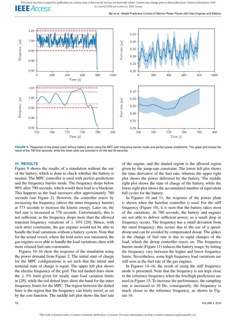
FIGURE 9. Response of the power plant without battery when using the MPC with frequency barrier mode and perfect power predictions. The upper plot shows theresult of the 790 first seconds, while the lower plots are zoomed-in on the last 50 seconds.

IV. RESULTSFigure 9 shows the results of a simulation without the useof the battery, which is done to check whether the battery isneeded. The MPC controller is used with perfect predictionsand the frequency barrier mode. The frequency drops below90% after 790 seconds, which would then lead to a blackout.This happens as the load increases after approximately 780seconds (see Figure 2). However, the controller reacts byincreasing the frequency (above the inner frequency barrier)at 773 seconds to increase the kinetic energy. Later on, thefuel rate is increased at 778 seconds. Unfortunately, this isnot sufficient, as the frequency drops more than the allowedtransient frequency variations of ± 10% [29]. Hence, withsuch strict constraints, the gas engines would not be able tohandle the load variations without a battery system. Note thatfor the actual vessel, where the load series was measured, thegas engines were able to handle the load variations, then withmore relaxed fuel rate constraints.

Figures 10–16 show the response of the simulation usingthe power demand from Figure 2. The initial state of chargefor the MPC configurations is set such that the initial andterminal state of charge is equal. The upper left plot showsthe electric frequency of the grid. The red dashed lines showthe ± 5% limit given for steady state load variation limitsin [29], while the red dotted lines show the band for the innerfrequency limits for the MPC. The region between the dottedlines is the region that the frequency can freely travel, as setby the cost function. The middle left plot shows the fuel rate

of the engine, and the shaded region is the allowed regiongiven by the jump-rate constraint. The lower left plot showsthe time derivative of the fuel rate, whereas the upper rightplot shows the power delivered by the battery. The middleright plot shows the state of charge of the battery, while thelower right plot shows the accumulated number of equivalentfull cycles for the battery.

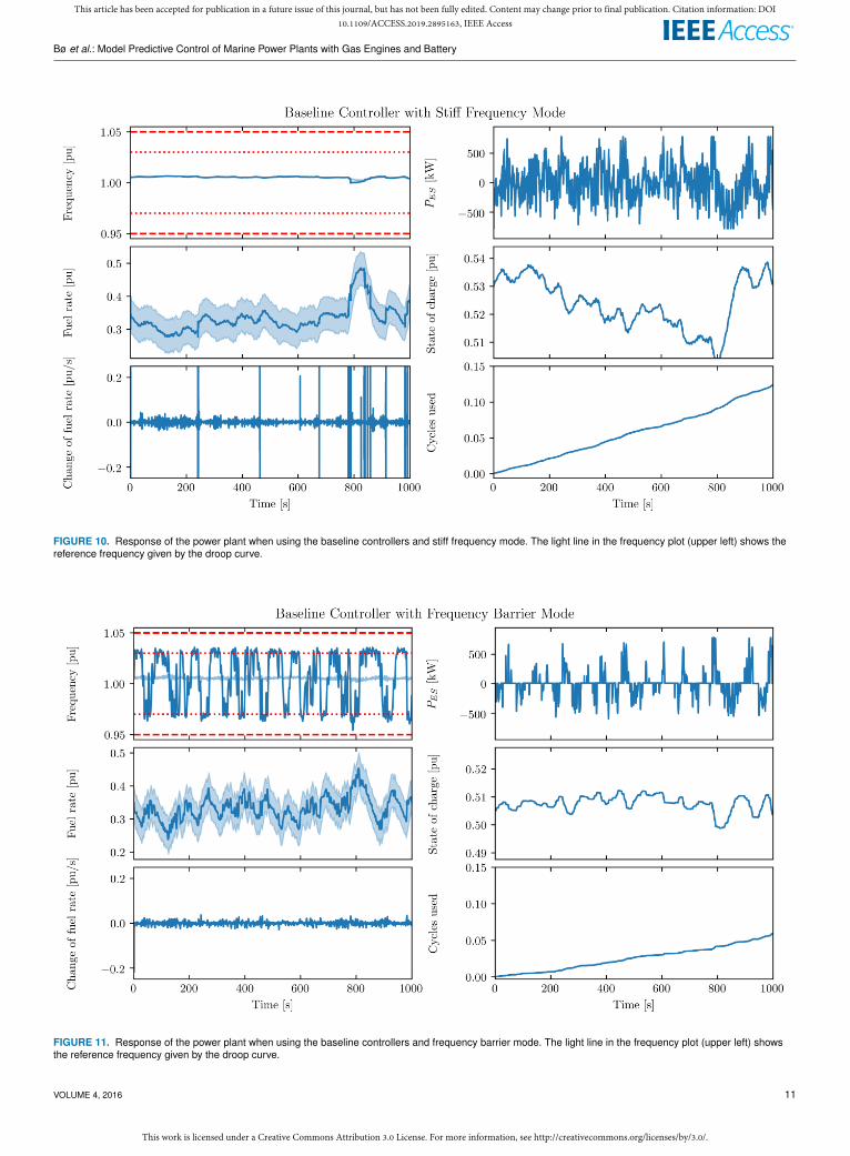
In Figures 10 and 11, the response of the power plantis shown when the baseline controller is used. For the stifffrequency (Figure 10), it is seen that the battery takes mostof the variations. At 780 seconds, the battery and enginesare not able to deliver sufficient power, so a small drop infrequency occurs. The frequency has a small deviation fromthe rated frequency; this occurs due to the use of a speed-droop and can be avoided by compensated droop. The spikesin the change of fuel rate is due to rapid changes of theload, which the droop controller reacts on. The frequencybarrier mode (Figure 11) reduces the battery usage, by lettingthe frequency vary between the higher and lower frequencylimits. Nevertheless, some high frequency load variations arestill seen in the fuel rate of the gas engines.

In Figures 14–16, the result of using the stiff frequencymode is presented. Note that the frequency is not kept closeto the reference frequency when the low/high predictions areused in Figure 15. To increase the performance, the samplingrate is increased to 10 Hz; consequently, the frequency ismuch closer to the reference frequency, as shown in Fig-ure 16.

10 VOLUME 4, 2016




FIGURE 10. Response of the power plant when using the baseline controllers and stiff frequency mode. The light line in the frequency plot (upper left) shows thereference frequency given by the droop curve.

FIGURE 11. Response of the power plant when using the baseline controllers and frequency barrier mode. The light line in the frequency plot (upper left) showsthe reference frequency given by the droop curve.

VOLUME 4, 2016 11




FIGURE 12. Response of the power plant when using the MPC with frequency barrier mode and perfect predictions

TABLE 3. The table shows the number of equivalent full cycles the battery iscycled if the load series is repeated for 10 years. The batteries are expected tolast for 10 years, and withstand 12,000 cycles. The energy loss in the batteryis also included in the table. It is given as the ratio between lost energy in thebattery due to ohmic losses and the total consumed energy by the consumers.The root mean square of u is shown in the right-hand column.

Mode Cyclesafter

10 years

Energyloss

RMS u[%/s]

Frequency barrier, baseline 18,684 0.2% 0.77

Stiff frequency, baseline 38,968 0.5% 30

Frequency barrier, perfect predic-tion

10,920 0.04% 0.28

Frequency barrier, low/high predic-tion

28,032 0.3% 0.37

Stiff frequency, perfect prediction 29,136 0.3% 0.32Stiff frequency, low/high prediction 39,672 0.5% 0.75Stiff frequency, low/high predic-tions, 10 Hz

39,000 0.5% 0.28

The resulting cycling is shown in Table 3. It shows thenumber of equivalent full cycles if this load series wascontinuously repeated for 10 years.

V. DISCUSSIONA. BASELINE CONTROLLER VS. MPCThe baseline controller gives an acceptable response. Forthe stiff frequency mode, the frequency is kept at a constantfrequency, with the exception of one frequency deviation dueto a load increase. The frequency barrier mode reduces the

use of the battery, while keeping the frequency within thegiven limits.

However, the MPC can improve the performance further.For the stiff frequency mode, the MPC can reduce the varia-tions of the fuel rate significantly, both for perfect predictionsand low/high predictions, with a 10 Hz sampling frequency.In addition, if perfect predictions are available, the numberof equivalent cycles is reduced by 25% and the frequencydeviation is avoided.

For the frequency barrier mode, variations in the fuelrate are reduced by using MPC. If perfect predictions areavailable, the number of equivalent cycles is reduced by 41%.

Note that the baseline controller uses distributed control,whereas the MPC is centralized. Reliability is highly im-portant for vessels with dynamic positioning system. Thedisadvantage with a centralized controller is that the systemis vulnerable to a single failure in the main controller, sodistributed control schemes are therefore often preferred.Thus, a backup controller may be used in cases where theMPC fails. For example, this can be the suggested baselinecontroller with the stiff frequency mode. The battery canalso implement the dead-band controller, which dischargesif the frequency is too low or charges if the frequency istoo high. This will distribute some safety functions. Yet,it should be noted that a distributed system may also fail.For instance, a locked fuel rate on an engine may cause anoverload or reverse power. Hence, reliability is a concern forboth distributed and centralized control schemes.

12 VOLUME 4, 2016




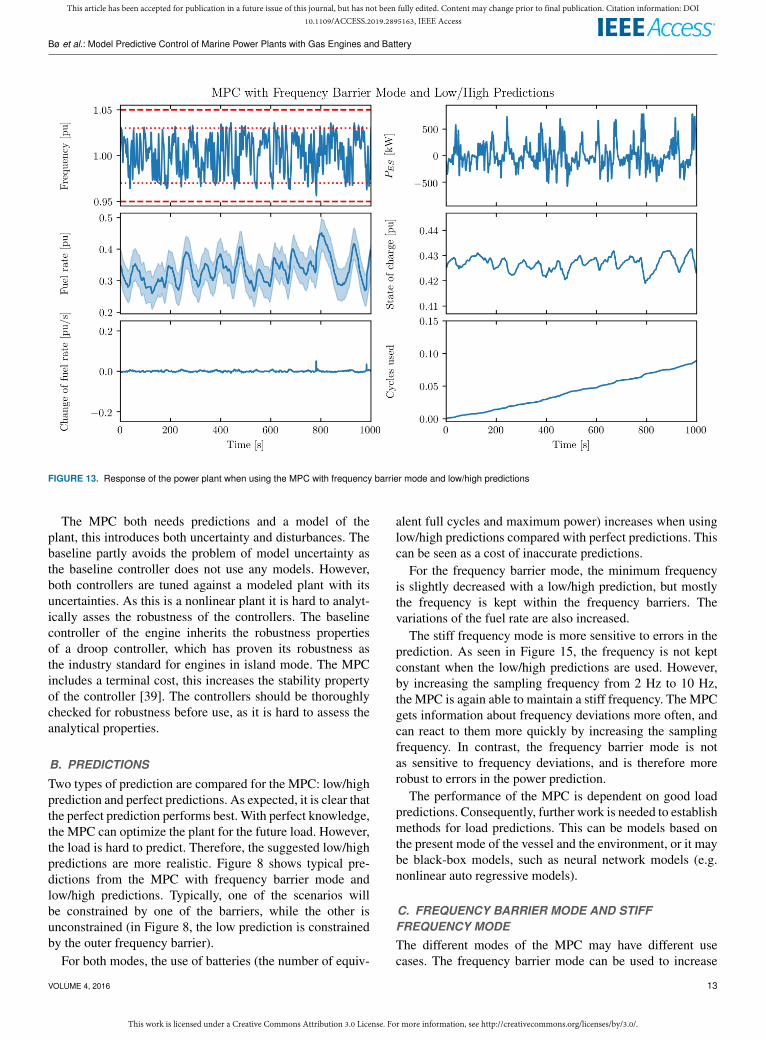
FIGURE 13. Response of the power plant when using the MPC with frequency barrier mode and low/high predictions

The MPC both needs predictions and a model of theplant, this introduces both uncertainty and disturbances. Thebaseline partly avoids the problem of model uncertainty asthe baseline controller does not use any models. However,both controllers are tuned against a modeled plant with itsuncertainties. As this is a nonlinear plant it is hard to analyt-ically asses the robustness of the controllers. The baselinecontroller of the engine inherits the robustness propertiesof a droop controller, which has proven its robustness asthe industry standard for engines in island mode. The MPCincludes a terminal cost, this increases the stability propertyof the controller [39]. The controllers should be thoroughlychecked for robustness before use, as it is hard to assess theanalytical properties.

B. PREDICTIONS

Two types of prediction are compared for the MPC: low/highprediction and perfect predictions. As expected, it is clear thatthe perfect prediction performs best. With perfect knowledge,the MPC can optimize the plant for the future load. However,the load is hard to predict. Therefore, the suggested low/highpredictions are more realistic. Figure 8 shows typical pre-dictions from the MPC with frequency barrier mode andlow/high predictions. Typically, one of the scenarios willbe constrained by one of the barriers, while the other isunconstrained (in Figure 8, the low prediction is constrainedby the outer frequency barrier).

For both modes, the use of batteries (the number of equiv-

alent full cycles and maximum power) increases when usinglow/high predictions compared with perfect predictions. Thiscan be seen as a cost of inaccurate predictions.

For the frequency barrier mode, the minimum frequencyis slightly decreased with a low/high prediction, but mostlythe frequency is kept within the frequency barriers. Thevariations of the fuel rate are also increased.

The stiff frequency mode is more sensitive to errors in theprediction. As seen in Figure 15, the frequency is not keptconstant when the low/high predictions are used. However,by increasing the sampling frequency from 2 Hz to 10 Hz,the MPC is again able to maintain a stiff frequency. The MPCgets information about frequency deviations more often, andcan react to them more quickly by increasing the samplingfrequency. In contrast, the frequency barrier mode is notas sensitive to frequency deviations, and is therefore morerobust to errors in the power prediction.

The performance of the MPC is dependent on good loadpredictions. Consequently, further work is needed to establishmethods for load predictions. This can be models based onthe present mode of the vessel and the environment, or it maybe black-box models, such as neural network models (e.g.nonlinear auto regressive models).

C. FREQUENCY BARRIER MODE AND STIFFFREQUENCY MODEThe different modes of the MPC may have different usecases. The frequency barrier mode can be used to increase

VOLUME 4, 2016 13




FIGURE 14. Response of the power plant when using the MPC with stiff frequency mode and perfect predictions

FIGURE 15. Response of the power plant when using the MPC with stiff frequency mode and low/high predictions

14 VOLUME 4, 2016




FIGURE 16. Response of the power plant when using the MPC with stiff frequency mode, low/high predictions and an increased sampling frequency (10 Hz)

the performance of the gas engine as the load variations onthe gas engine are reduced. In addition, the battery usage isreduced, and the battery may be downsized as the peak powerdemand is decreased.

The stiff frequency mode may be used when a fixedfrequency is needed, which is required when a new generatoris synchronized to the grid. For DP operations reliability ishighly important. For this reason, the stiff frequency modemay then be preferred. One advantage is that faults may beeasier to detect when a stiff frequency is used, as a majordeviation of the frequency indicates that a fault exists inthe system. Another advantage is that this gives the largestfrequency margin, which also gives a safety margin.

D. BATTERY SIZE AND AGING

In Table 3, the number of equivalent full cycles is shown.This is calculated by using the same load series for 10 years.The number of equivalent full cycles is more than three timesthe rated 12,000 cycles of the battery for many of the modes.However, this is a conservative estimate since the vessel willonly be used in harsh DP operations for a short time duringthe 10 year lifetime of the batteries. In [40], it is reportedthat the vessel is only in dynamic positioning operations 35%of the time and only a portion of this is in harsh weather.Moreover, the batteries are rated for 15,000 cycles, with adepth of discharge (DoD) of 80% (12,000 equivalent fullcycles) [31]. Even so, it is reported that the aging of an NMCcell due to an equivalent full cycle is much larger for a large

DoD, compared with a small DoD [41].

The batteries may therefore be used for additional usecases, such as "spinning reserve." The batteries used in thissimulation are able to deliver 780 kW for 20 minutes andcan be used to power thruster units during DP operation [29,Pt. 6, Ch. 3., Sec. 8.3]. One usage is that the vessel uses onegenerator set to produce power, and has a battery ready inbackup; this is called "spinning reserve." The battery mustthen be able to supply sufficient power and energy to safelyterminate the current DP operation in the event of a suddendisconnection of the running generator. With this battery, thevessel can run with the battery for "spinning reserve" whenthe load is small (e.g. in calm weather).

Note that only a small portion of the total energy of the bat-tery is used (max SoC-min SoC). The frequency barrier modewith perfect predictions uses only 1.6 kWh, while the stifffrequency mode with low/high predictions uses 4.8 kWh. Thedimensioning factor is therefore the power, not the energy.One alternative would thus be to use ultra capacitors (UC),which have a high power rating, but a low energy capacity.The power capacity of UC is proportional to the voltage.Using 49 UC modules of type "125V Heavy TransportationModules" from Maxwell gives 5 kWh of useful energy and aminimum power of 794 kW (minimum voltage of 54%) [42].The weight will be approximately 3,000 kg (slightly less thanthe 3,800 kg of the suggested battery pack). For the config-uration with MPC, the stiff frequency mode and a low/highprediction, 1.46 million equivalent full cycles would be used

VOLUME 4, 2016 15




by the ultra capacitor. The rated number of cycles is 1 millionequivalent full cycles or 10 years of operation.

As noted earlier, the energy buffer of the generator setsis 667 Wh in total. This energy buffer is utilized in thefrequency barrier mode. The energy storage requirement istherefore on the order of 3–10 times larger than the kineticenergy storage of the generator set. Note that a larger kineticenergy storage is available if the engines can use a variablefrequency (e.g. direct current grid). In these cases, the fre-quency may vary from 60% to 110%, which increases thekinetic energy storage up to 1.4 kWh. However, at a 60%speed, the power of the engine and generator is reduced to60% as the torque is limited. Simulation has shown (not pre-sented due to page limitations) that a battery is also neededif the speed can drop to 60%. Typically, a load increase willreduce the speed, and hence the available power, from thegenerator set. Moreover, a large frequency span can furtherdecrease the number of equivalent cycles.

VI. CONCLUSIONA control method based on model predictive control (MPC)to control an Otto-cycle gas engine and a battery is presented.The controller is compared with a baseline controller, wherethe generator sets are controlled by speed-droop. For thebaseline controller, the battery is controlled as a virtualgenerator.

The methods are compared by a simulation study, in whicha real-world time series of power demand for a DP vesselin a 3 m wave height is used. The MPC is tested with twodifferent power load predictions: either that it uses a highand low scenario for the load, or has perfect knowledge ofthe upcoming power demand. Two configurations of the costfunction are used. One configuration allows the frequencyto stay within a band, and has a high cost on the use ofthe battery. A second configuration has a large penalty onfrequency deviations, though use of the battery is cheap.

The simulation shows that the MPC is able to maintaina slowly varying load on the generator set, or keeps thefrequency constant if the MPC has perfect knowledge ofthe upcoming power or a high sample rate is used. Theperformance is degraded if the future power is unknown. Thismotivates for further studies on predictions of the short-termpower demand of marine vessels.

The lifetime of the battery is also evaluated. The batteriesare expected to last for 3 to 10 years of operation with DPharsh weather only. The method seems to be implementable,as the vessel is only in this condition for a small part of the10-year expected lifetime of the battery.

REFERENCES[1] V. Shagar, S. G. Jayasinghe, and H. Enshaei, “Effect of Load Changes

on Hybrid Shipboard Power Systems and Energy Storage as a PotentialSolution: A Review,” Inventions, vol. 2, no. 3, p. 21, 2017. [Online].Available: http://www.mdpi.com/2411-5134/2/3/21

[2] T. W. P. Smith, J. P. Jalkanen, B. A. Anderson, J. J. Corbett, J. Faber,S. Hanayama, E. O’Keeffe, S. Parker, L. Johansson, L. Aldous, C. Raucci,M. Traut, S. Ettinger, D. Nelissen, D. S. Lee, S. Ng, A. Agrawal, J. J.

Winebrake, and A. Hoen, M., “Third IMO Greenhouse Gas Study 2014,”International Maritime Organization (IMO), p. 327, 2014.

[3] T. Smith, C. Raucci, S. Haji Hosseinloo, I. Rojon, J. Calleya, S. Suarezde la Fuente, P. Wu, and K. Palmer, “CO2 Emissions from InternationalShipping: Possible reduction targets and their associated pathways,” Tech.Rep., 2016.

[4] V. Æsøy, P. Magne Einang, D. Stenersen, E. Hennie, and I. Valberg,“LNG-fuelled engines and fuel systems for medium-speed engines inmaritime applications,” in SAE International Powertrains, Fuels andLubricants Meeting. SAE International, Aug. 2011. [Online]. Available:https://doi.org/10.4271/2011-01-1998

[5] C. Wang, M. H. Nehrir, and S. R. Shaw, “Dynamic models and modelvalidation for pem fuel cells using electrical circuits,” IEEE Transactionson Energy Conversion, vol. 20, no. 2, pp. 442–451, June 2005.

[6] B. Zahedi, L. E. Norum, and K. B. Ludvigsen, “Optimized efficiency ofall-electric ships by dc hybrid power systems,” Journal of Power Sources,vol. 255, no. Supplement C, pp. 341–354, 2014. [Online]. Available:http://www.sciencedirect.com/science/article/pii/S0378775314000469

[7] E. Ovrum and T. Bergh, “Modelling lithium-ion batteryhybrid ship crane operation,” Applied Energy, vol. 152, no.Supplement C, pp. 162 – 172, 2015. [Online]. Available:http://www.sciencedirect.com/science/article/pii/S0306261915001026

[8] “Hybrid power system makeover for balticsea ferry,” online, May 2013. [Online]. Avail-able: http://articles.maritimepropulsion.com/article/Largest-Hybrid-Power-System-in-the-World-Installed-in-Danish-Ferry57461.aspx

[9] E. Skjong, E. Rødskar, M. Molinas, T. A. Johansen, and J. Cunningham,“The marine vessel’s electrical power system: From its birth to presentday,” Proceedings of the IEEE, vol. 103, no. 12, pp. 2410–2424, Dec. 2015.

[10] F. Lambert, “Two massive ferries are about to become the biggestall-electric ships in the world,” online, August 2017. [Online]. Available:https://electrek.co/2017/08/24/all-electric-ferries-abb/

[11] “A first-hand look at rt adriaan,” online, September 2013. [Online].Available: http://www.maritimejournal.com/news101/tugs,-towing-and-salvage/a-first-hand-look-at-rt-adriaan

[12] “Electric asv awarded,” online, June 2017. [On-line]. Available: http://www.maritimejournal.com/news101/power-and-propulsion/electric-asv-awarded

[13] “Pioneering battery hybrid ferry launches infjords,” online, July 2016. [Online]. Available:http://www.passengership.info/news/view,pioneering-battery-hybrid-ferry-launches-in-fjords_43774.htm

[14] “Energy storage systems,” online, visited 28.09.2017, 2017. [On-line]. Available: http://new.abb.com/marine/systems-and-solutions/power-generation-and-distribution/energy-storage

[15] X. Hu, C. Zou, C. Zhang, and Y. Li, “Technological developments inbatteries: A survey of principal roles, types, and management needs,” IEEEPower and Energy Magazine, vol. 15, no. 5, pp. 20–31, Sept 2017.

[16] S. Kanerva, P. Pohjanheimo, and M. Kajava, “Dynamic ac concept,” ABB,Tech. Rep., 2016.

[17] J. Hou, J. Sun, and H. F. Hofmann, “Mitigating power fluctuations inelectric ship propulsion with hybrid energy storage system: Design andanalysis,” IEEE Journal of Oceanic Engineering, vol. PP, no. 99, pp. 1–15,2017.

[18] J. Hou, J. Sun, and H. Hofmann, “Battery/flywheel hybrid energy storageto mitigate load fluctuations in electric ship propulsion systems,” in 2017American Control Conference (ACC), May 2017, pp. 1296–1301.

[19] W. Chen, A. K. Ådnanses, J. F. Hansen, J. O. Lindtjørn, and T. Tang,“Super-capacitors based hybrid converter in marine electric propulsionsystem,” in The XIX International Conference on Electrical Machines -ICEM 2010, Sept. 2010, pp. 1–6.

[20] T. I. Bø and T. A. Johansen, “Battery power smoothing control in amarine electric power plant using nonlinear model predictive control,”IEEE Transactions on Control Systems Technology, vol. 25, no. 4, pp.1449–1456, July 2017.

[21] A. Haseltalab, R. R. Negenborn, and G. Lodewijks, “Multi-LevelPredictive Control for Energy Management of Hybrid Ships inthe Presence of Uncertainty and Environmental Disturbances,” in14th IFAC Symposium on Control in Transportation SystemsCTS2016, vol. 49, no. 3. Elsevier B.V., 2016, pp. 90–95. [Online]. Available: http://dx.doi.org/10.1016/j.ifacol.2016.07.016http://linkinghub.elsevier.com/retrieve/pii/S2405896316302129

[22] S. A. M. Al-Barazanchi and A. M. Vural, “Modeling and intelligentcontrol of a stand-alone pv-wind-diesel-battery hybrid system,” in 2015

16 VOLUME 4, 2016




International Conference on Control, Instrumentation, Communicationand Computational Technologies (ICCICCT), Dec. 2015, pp. 423–430.

[23] D. C. Das, A. K. Roy, and N. Sinha, “PSO based frequency controllerfor wind-solar-diesel hybrid energy generation/energy storage system,” in2011 International Conference on Energy, Automation and Signal, Dec.2011, pp. 1–6.

[24] S. Barsali, C. Miulli, and A. Possenti, “A Control Strategy to MinimizeFuel Consumption of Series Hybrid Electric Vehicles,” IEEE Transactionson Energy Conversion, vol. 19, no. 1, pp. 187–195, 2004.

[25] S. M. Lukic, S. G. Wirasingha, F. Rodriguez, J. Cao, and A. Emadi, “Powermanagement of an ultracapacitor/battery hybrid energy storage system inan hev,” in 2006 IEEE Vehicle Power and Propulsion Conference, Sept.2006, pp. 1–6.

[26] A. Brahma, Y. Guezennec, and G. Rizzoni, “Optimal energy managementin series hybrid electric vehicles,” in Proceedings of the 2000 AmericanControl Conference. ACC (IEEE Cat. No.00CH36334), vol. 1, no. 6, Sept.2000, pp. 60–64 vol.1.

[27] E. Vaktskjold, L.-A. Skarbo, K. Valde, K. S. Foer, T. Humerfelt, R. Nord-vik, and B. O. Bruvik, “The new bergen B35:40 lean burn marine gasengine serie and practical experiences of SI lean burn gas engines formarine mechanical drive,” Proceedings of the 25th CIMAC Congress.Shanghai, 2013.

[28] T. I. Bø, A. R. Dahl, T. A. Johansen, E. Mathiesen, M. R. Miyazaki,E. Pedersen, R. Skjetne, A. J. Sørensen, L. Thorat, and K. K. Yum, “Marinevessel and power plant system simulator,” IEEE Access, vol. 3, pp. 2065–2079, 2015.

[29] “Rules for classification: Ships,” DNV GL, Tech. Rep., January 2017.[30] PBES, “PBES specification sheet,” Online, visited 28.08.2017., datasheet.[31] “XaltTM75 Ah high power (HP) superior lithium ion

cell,” Datasheet, September 2014, datasheet number:09_09_2014_XALT_Energy_75AH_HP_Spec_Sheet.

[32] T. I. Bø and T. A. Johansen, “Scenario-based fault-tolerant model predic-tive control for diesel-electric marine power plant,” in 2013 MTS/IEEEOCEANS - Bergen, June 2013, pp. 1–5.

[33] J. J. May, “Improving engine utilization on DP drilling vessels,” in Dy-namic Positioning Conference, 2003.

[34] A. M. Ersdal, L. Imsland, K. Uhlen, D. Fabozzi, and N. F.Thornhill, “Model predictive load–frequency control taking intoaccount imbalance uncertainty,” Control Engineering Practice, vol. 53,no. Supplement C, pp. 139 – 150, 2016. [Online]. Available:http://www.sciencedirect.com/science/article/pii/S0967066115300496

[35] B. Houska, H. Ferreau, and M. Diehl, “An Auto-Generated Real-TimeIteration Algorithm for Nonlinear MPC in the Microsecond Range,”Automatica, vol. 47, no. 10, pp. 2279–2285, 2011.

[36] H. P. Beck and R. Hesse, “Virtual synchronous machine,” 2007 9th Inter-national Conference on Electrical Power Quality and Utilisation, EPQU,2007.

[37] H. Bevrani, T. Ise, and Y. Miura, “Virtual synchronous generators: Asurvey and new perspectives,” International Journal of Electrical Powerand Energy Systems, vol. 54, pp. 244–254, 2014. [Online]. Available:http://dx.doi.org/10.1016/j.ijepes.2013.07.009

[38] Q. C. Zhong and G. Weiss, “Synchronverters: Inverters that mimic syn-chronous generators,” IEEE Transactions on Industrial Electronics, vol. 58,no. 4, pp. 1259–1267, 2011.

[39] L. Grüne and J. Pannek, Nonlinear Model Predictive Control. Springer,2011.

[40] T. I. Bø, A. Swider, and E. Pedersen, “Investigation of drivetrain losses of adp vessel,” in 2017 IEEE Electric Ship Technologies Symposium (ESTS),Aug. 2017, pp. 508–513.

[41] M. Ecker, N. Nieto, S. Käbitz, J. Schmalstieg, H. Blanke,A. Warnecke, and D. U. Sauer, “Calendar and cycle life studyof Li(NiMnCo)O2-based 18650 lithium-ion batteries,” Journal ofPower Sources, vol. 248, pp. 839–851, 2014. [Online]. Available:http://dx.doi.org/10.1016/j.jpowsour.2013.09.143

[42] Maxwell, “125v heavy transportation module,” Online, visited28.08.2017., datasheet, document number 1014696.7.

VOLUME 4, 2016 17

Documents

Model Predictive Control of Marine Power Plants with Gas