Embed Size (px)
Citation preview

DIPARTIMENTODI INGEGNERIADELL'INFORMAZIONE
Model Predictive Control of HVAC Systems:Design and Implementation on a Real Case Study
Laureando
Giorgio Pattarello
Relatore
Prof. Ruggero Carli
Correlatore
Prof. Karl H. Johansson
Dipartimento di
Ingegneria
dell’Informazione
Anno 2013

Abstract
Recently, one of the most debated subjects regards energy savings. Since the
percentage of the energy consumptions accounted for buildings is surprisingly
higher than the one for the industries and transportations, the society is
becoming more and more aware of the importance of the quality of building
management. This gives an impulse to the automatic control community to
design intelligent controllers for energy savings, a fact that appears evident also
in the scientific literature. Many efforts have been spent in order to propose
different control technique for the HVAC systems. However, only few papers
deal with the implementation and test of the proposed controllers on a real
case study. There is thus still the need of understanding what is critical in
the implementation of such schemes, what affects the most the energy saving
possibilities, and what is the critical and valuable information.
The final aim of this work is thus to design, implement and test a controller
on a real testbed kindly provided by KTH Royal Institute of Technology. The
control paradigm presented in this thesis is a model predictive controller that
aims at saving energy as well as keeping the temperature and the carbon
dioxide (CO2) concentration in a comfort range that guarantees the wellness
of room occupants. To improve the knowledge of the plant, we also study the
problem of modeling both the dynamics of the system to be controlled and
of the dedicated actuation system. Our experiments show that the obtained
controller is able to satisfy the requests on energy savings and comfort, and
hence can be used as a starting point for the design of efficient model based
controllers of HVAC systems.

ii

Acknowledgements
The path I walked on to get to where I am now has been very long and twisting
but all the people I found along made my travel easier and enjoyable. From
all of them I have learnt something that I will always carry with me. In this
occasion I can write on paper how grateful I am to them.
First of all I would like to thank Prof. Ruggero Carli and Prof. Karl Henrik
Johansson for having given me the opportunity to spend six beautiful months in
Stockholm, learning, growing and enjoying. Without this experience probably
I would not have been aware of some aspect of the life that sometimes after a
while you may forget.
Thanks to Damiano, Alessandra, Marco an also Giulio for having been so
patient, willing and kind with me in all the period I spent both inside and
outside the department; in particular Damiano has been for me more than a
supervisor and he helped me every time I had any kind of problem.
I want to thank also my parents and my sister. They always supported,
trusted and believed in me in all the choices I have done in my life.
Thanks to Coba, Zano, Gamba, Guido and Michele for having been always
real and honest friends. Especially I want to thank Coba and Marta for the
big role they gave me in a very remarkable day of their life. I am very proud
of this, and I am very proud of you all. I wish you all the best in your future
because you deserve it.
Thanks to Valerio, Giulio, Demia and Alberto for making me feel in a family
all the time. The time I spent with you was really great.
Thanks to all the HVAC group, especially Lin, Mani, Daniel, Ferran, Alireza,
Afrooz and all the people who helped me and shared with me the technical
problems of a real testbed; thanks also to Akademiska Hus for the support for
the measurements.
Thanks to Andrea, Gianluca, Giacomo, Lorenza, Giulia M., Giulia V.,

iv
Laura, Elena, all my past teammates and all the people with whom I shared
also a little part of my life, because I will always have a little piece of you in
me.
Thanks to Volpe and Lanza for having shared with me most of the troubles
I have had to become an engineer.
I leave at the end a very special thanks for my grandparents. They have
been like parents for me in all my life, they were always ready to help me and
my family in every occasion they had. I owe you a lot.
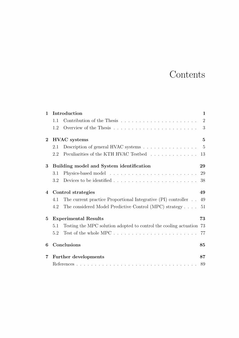
Contents
1 Introduction 1
1.1 Contribution of the Thesis . . . . . . . . . . . . . . . . . . . . . 2
1.2 Overview of the Thesis . . . . . . . . . . . . . . . . . . . . . . . 3
2 HVAC systems 5
2.1 Description of general HVAC systems . . . . . . . . . . . . . . . 5
2.2 Peculiarities of the KTH HVAC Testbed . . . . . . . . . . . . . 13
3 Building model and System identification 29
3.1 Physics-based model . . . . . . . . . . . . . . . . . . . . . . . . 29
3.2 Devices to be identified . . . . . . . . . . . . . . . . . . . . . . . 38
4 Control strategies 49
4.1 The current practice Proportional Integrative (PI) controller . . 49
4.2 The considered Model Predictive Control (MPC) strategy . . . . 51
5 Experimental Results 73
5.1 Testing the MPC solution adopted to control the cooling actuation 73
5.2 Test of the whole MPC . . . . . . . . . . . . . . . . . . . . . . . 77
6 Conclusions 85
7 Further developments 87
References . . . . . . . . . . . . . . . . . . . . . . . . . . . . . . . . . 89

vi Contents

List of Figures
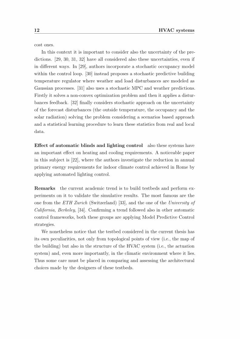
2.1 External view of the Q building in Stockholm, Sweden. The
building is composed by 7 floors, from floor 2 to floor 8. Floor 2,
that is actually the first floor, is underground. . . . . . . . . . . 13
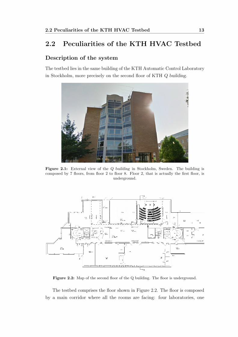
2.2 Map of the second floor of the Q building. The floor is underground. 13
2.3 Diagram of the actuation systems present in the water tank lab.
This scheme shows the degrees of freedom and the constraints
that must be faced when designing air quality control schemes
for the considered testbed. . . . . . . . . . . . . . . . . . . . . . 15
2.4 Map showing the temperature of the water flowing through
the radiators as a function of the external temperature. The
map represents reference temperatures, since it neglects all the
possible dynamics on these quantities. . . . . . . . . . . . . . . . 16
2.5 Photos of one of the radiators, the fresh air inlet, the exhausted
air outlet and the air conditioning outlet present in the water
tank lab. . . . . . . . . . . . . . . . . . . . . . . . . . . . . . . . 16
2.6 Scheme of the air inlets present in the water tank lab. . . . . . . 17
2.7 Scheme of the air conditioning system of the water tank lab. . . 18
2.8 SCADA interface of the system that provides the fresh air to
the venting and cooling system . . . . . . . . . . . . . . . . . . 20
2.9 A Tmote Sky with highlighted the various measurements systems. 21
2.10 Tipical star network topology, it is used also in our network . . 22
2.11 Map of the sensors deployed in the Kungliga Tekniska H ogskolan
- Royal Institute of Technology (KTH) testbed . . . . . . . . . . 22
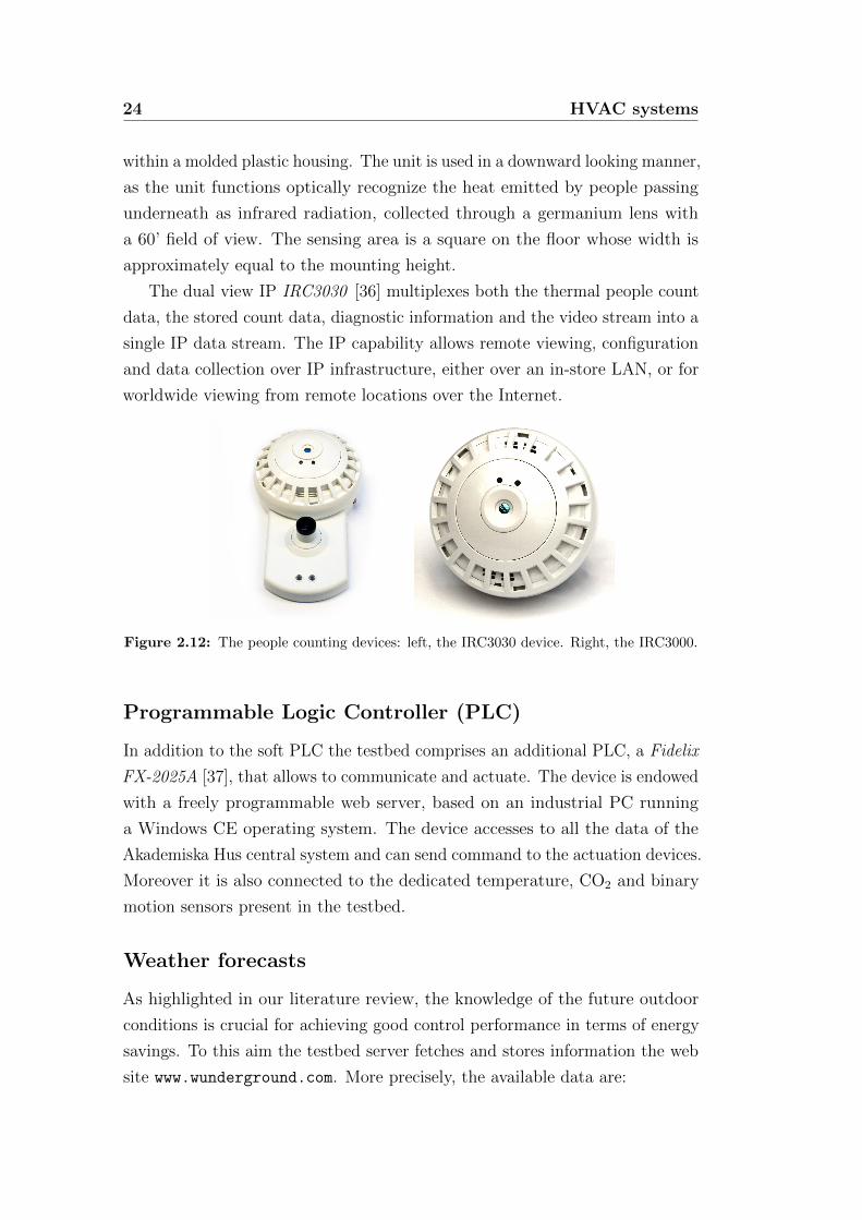
2.12 The people counting devices: left, the IRC3030 device. Right,
the IRC3000. . . . . . . . . . . . . . . . . . . . . . . . . . . . . 24
viii List of Figures
2.13 A scheme representing the whole testbed system; LabVIEW is
the tool that allow the user to communicate with the whole
network by a collection of virtual instruments. . . . . . . . . . . 25
2.14 The web interface that allows every single user to download the
sensed data and the actuation command of the system. . . . . . 27
3.1 Electric scheme of the model of the walls. The three resistances
1/ho, Rjwall and 1/hi are placed between the equivalent temper-
ature T jee, and the temperatures T j
wall,o, Tjwall,i and Troom. Rj
wall
[°C/W] and C j [J/°C] are the thermal resistance and the thermal
capacity of the j-th wall respectively . . . . . . . . . . . . . . . 32
3.2 Validation of the model performed with the software IDA ICE. . 32
3.3 Comparison between the simulated temperatures obtained with
the physical model and the actual measured room temperature. 33
3.4 Validation of the CO2 physical model. . . . . . . . . . . . . . . . 34
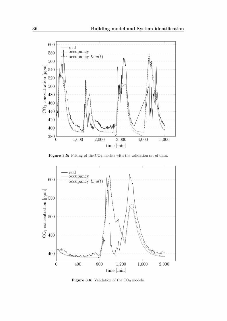
3.5 Fitting of the CO2 models with the validation set of data. . . . 36
3.6 Validation of the CO2 models. . . . . . . . . . . . . . . . . . . . 36
3.7 Picture of the motes attached to the radiator to run the test to
get the mean radiant temperature. . . . . . . . . . . . . . . . . 39
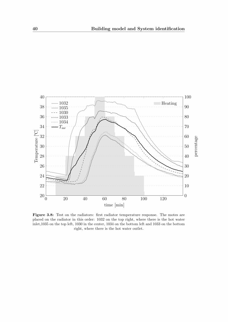
3.8 Test on the radiators: first radiator temperature response. The
motes are placed on the radiator in this order: 1032 on the top
right, where there is the hot water inlet,1035 on the top left,
1030 in the center, 1034 on the bottom left and 1033 on the
bottom right, where there is the hot water outlet. . . . . . . . . 40
3.9 Test on the radiators: Comparison between motes in the first
radiator (1035, 1030) and in the last (1036, 1037), placed in the
same position on the radiator. Motes 1035 and 1036 are placed
on the top left corner of the first and last radiator respectively,
while Sensor 1030 and Sensor 1037 are placed in the center. . . . 41
3.10 Relation between mass flow and opening valve percentage . . . . 44
3.11 Fitting between real supply air temperature of the air condition-
ing outlet and the simulated one. . . . . . . . . . . . . . . . . . 46
4.1 Example of the actuation signals induced by the Akademiska
Hus PI controller: cooling action. . . . . . . . . . . . . . . . . . 50
4.2 Basic description of the main functioning of a Model Predictive
Control (MPC) scheme [44]. . . . . . . . . . . . . . . . . . . . . 54
List of Figures ix
5.1 Simulation on the second level MPC for the Tsa. The reference
is set to 17 the ventilation is constant at 30%. . . . . . . . . . 74
5.2 Simulation on the second level MPC for the Tsa. The reference
is set to 18 the ventilation is constant at 30%. . . . . . . . . . 74
5.3 Test on the equilibrium point method for the Tsa. The reference
is set to 17 and the ventilation is constant at 30%. . . . . . . 75
5.4 Test on the equilibrium point method for the Tsa. The reference
is set to 18 and the ventilation is constant at 30%. . . . . . . 75
5.5 Test on the MPC for the Tsa. The reference is set to 17 and
the ventilation is constant at 30%. . . . . . . . . . . . . . . . . 76
5.6 Test on the MPC for the Tsa. The reference is set to 18 and
the ventilation is constant at 30%. . . . . . . . . . . . . . . . . 76
5.7 Test 1 on the MPC. The temperature comfort bounds are set to
20 to 23 while the upper bound of the CO2 concentration
is 700 ppm. . . . . . . . . . . . . . . . . . . . . . . . . . . . . . 80
5.8 Test 2 on the MPC. The temperature comfort bounds are set to
20 to 23 while the upper bound of the CO2 concentration
is 700 ppm. . . . . . . . . . . . . . . . . . . . . . . . . . . . . . 81
5.9 Test 3 on the MPC. The temperature comfort bounds are set to
20 to 23 while the upper bound of the CO2 concentration
is 700 ppm. . . . . . . . . . . . . . . . . . . . . . . . . . . . . . 82
5.10 Test 4 on the MPC. The temperature comfort bounds are set to
20 to 23 while the upper bound of the CO2 concentration
is 750 ppm. . . . . . . . . . . . . . . . . . . . . . . . . . . . . . 83

x List of Figures
1Introduction
Buildings account for a surprisingly high percentage of energy consumption.
As reported in [1], in 2004 the United States the management of buildings
consumed the 41% of the total energy spent by mankind. In the EU this figure
was reported to be 37% of the final energy, bigger than industry (28%) and
transportation (32%) . In the UK, the proportion of energy use in building is
39%, slightly above the European average.
Environmental concerns pair with the large and attractive opportunities that
exist to reduce buildings’ energy use. To give some figures, the International
Energy Agency’s (IEA) targets a 77% reduction in the planet’s carbon footprint
by 2050. At the same time reports by the World Business Council for Sustainable
Development (WBCSD) in 2009 suggest that the possibility of cutting the
energy consumptions in buildings is dramatic, comparable to the amount of
energy currently required by the entire transportation sector.
The vision of the mainstream researchers is that these energy savings can
be achieved by exploiting information, or, to use a buzz-word, by implementing
intelligent buildings. This means to control buildings using meaningfully the
data coming from the various information sources available now or in the near
future.
2 Introduction
This trend of “smartening the buildings” is already a current trend of
the next generation’s commercial buildings. For example, Building energy
and comfort management (BECM) systems are control systems for individual
buildings or groups of buildings that use computers and distributed micro-
processors for monitoring, storing data and implementing communications
between them. Since the average lifetime of a novel building ranges from 50
to 100 years, it is urgent to investigate how to build Heating, Venting and Air
Conditioning (HVAC) systems in order to enhance their capabilities.
The role of the Automatic Controls community is then to understand:
• what are the limitations of the state-of-the art control schemes;
• how these limitations can be overcome by means of information.
More precisely, the aim is to understand what kind of information is needed
to be energy efficient, and how to use it. For example, it might turn out
that having accurate weather forecasts is much more important than having
accurate buildings occupancy models, or that using MPC strategies does not
lead to significant energy savings with respect to simpler strategies such as
Proportional, Integrative and Derivatives (PIDs).
The current mainstream research is thus focusing on testing novel controllers
and inferring what is critical from an information point of view.
1.1 Contribution of the Thesis
This thesis follows the current trend of considering Model Predictive Control
(MPC) strategies. This control technique is popular mainly because of its
capability to handle multivariate variable problems as well as to incorporate
constraints for the manipulated and the controlled variables. It started being
adopted in building climate control frameworks for also other reasons: the first
is that the dynamics of buildings are usually slow, and this makes meaningful
the fact of exploiting predictions. Moreover the comfort ranges, i.e., the aim of
the control actions are precisely defined by European standards, helping thus
the formalization process.
When applied to buildings, MPC schemes must face the peculiarity that
building dynamics are highly affected by uncertainties. This implies that indoor
climate predictive controllers must cope with disturbance rejection problems,
the most being
1.2 Overview of the Thesis 3
• external weather conditions that do not follow exactly the forecasts
provided by weather forecast systems;
• rooms occupancy patterns that are usually unknown or highly non sta-
tionary in time;
• sudden and unexpected changing conditions, like opening / closing win-
dows or similar manual actions.
The role of this thesis is thus to analyze, standing on the shoulders of giants,
what affects MPC schemes in real HVAC systems. Thus to see, from practical
perspectives, what plays a critical role and what needs to be addressed in the
future to improve their energy-savings performance.
Specifically the thesis describes in details the implementation of MPC
schemes on a real testbed. By doing so we achieved some specific contributions,
that can be summarized in:
• design and perform modeling and system identification of radiators and
air ventilation systems. This with the aim of inferring the importance of
having accurate actuators models;
• tailor classical MPC schemes to a real HVAC testbed, and identify the
idealizations that are often assumed in literature. This aims to understand
how much the practical problems encountered during implementations
can lead to deviations from theoretical findings;
• perform comparisons with current practice controllers. This to have
at least rough indications of what are the advantages of implementing
advanced control schemes and what can actually be saved in terms of
energy consumptions.
1.2 Overview of the Thesis
The manuscript is organized as follows. In Chapter 2 we review the literature
related to the control of HVAC systems, introduce our case study and describe
our testbed in details. In Chapter 3 instead we present the models of our system
and the methodologies used to decipher the temporal behavior of the control-
related variables. In Chapter 4 we illustrate the control strategy adopted, after

4 Introduction
describing the general principles of MPC. In Chapter 5 we then picture the
results obtained implementing the previously analyzed controllers. In the two
final chapters 6 and 7, we eventually draw some conclusions and suggest some
possible prospects for further developments and improvements.
2HVAC systems
2.1 Description of general HVAC systems
An Heating, Venting and Air Conditioning (HVAC) system is a set of infras-
tructures, devices and actuators that are devoted to the conditioning of the air
in buildings, i.e., to the control of the temperature, humidity and CO2 levels.
This section presents a survey of the different technologies and methodologies
present in literature and in practice. We remark that a big part of the literature
is currently presenting simulative results that have actually never been tested
on real testbeds. Thus there is currently a gap between the current practice
and the theoretical studies performed by the various research groups.
General technologies used in HVAC systems
A common approach in the existing research projects on HVAC systems is
to perform data acquisition and user activity detection exploiting Wireless
Sensor Networks (WSNs). We notice that a general requirement is to use
simple, wireless, binary sensors since they are cheap, easy to retrofit in existing
buildings, require minimal maintenance and supervision, and do not require
6 HVAC systems
users to change their behavior, e.g., have to be worn or carried. This means
that doing research on HVAC systems requires to do not resort to any advanced
sensing technology that is expensive, generating privacy concerns or requiring
changes in user behavior, e.g., cameras, Radio Frequency Identification (RFID)
tags, or wearable sensors.
In a schematic way, the most used hardware tools are:
• temperature, humidity, light and CO2 sensors (wired, embedded on a
mote or soldered on a wireless sensors boards);
• acoustic sensors (also microphones);
• Passive Infrared (PIR) sensors (for motion detection or people counting);
• switch-door sensors (magnetic);
• cameras;
• RFID tags.
Simple sensors are used in many energy intelligent buildings in the interest of
activity recognition. For instance, PIR based sensors are often used (especially
with lighting system) for occupancy detection. The sensors are connected
directly to local lighting fixtures. These PIR sensors are also simple movement
sensors and often cannot actually determine if the room is occupied or not. E.g.,
if the persons stand still, they will fail in detecting the occupancy. PIR sensors
are used for instance in [2], where Padmanabh et al. investigate the joint use of
microphones and PIR sensors for inferring the scheduling of conference rooms.
An other project where PIR sensors have been used is the AIM Project [3],
where authors used sensors to get some physical parameters, like temperature
and light, as well as PIR to infer user presence in each room of a house.
Indoor activity recognition is in general implemented to provide inputs to a
control strategy that aims for energy savings in buildings. To this aim, other
sensors than PIRs can be used: in Greener Building [4] authors perform indoor
activity recognition using simple infrared, pressure and acoustic sensors. An
other strategy is to use door sensors. For instance [5] uses them in conjunc-
tion with PIR sensors to automatically turn off the HVAC system when the
occupants are sleeping or away from home. Also in [6] Agarwal et al. chose
to use a combination of a magnetic reed switch door sensor and a PIR sensor
2.1 Description of general HVAC systems 7
module to build their building occupancy model. An even more complete
testbed has been constructed in ARIMA [7]. Here, to gather data related to
total building occupancy, wireless sensors are installed in a three-story building
in eastern Ontario (Canada) comprising laboratories and 81 individual work
spaces. Contact closure sensors are placed on various doors, PIR motion sensors
are placed in the main corridor on each floor, and a carbon-dioxide sensor
is positioned in a circulation area. In addition, the authors collect data on
the number of people who log in to the network on each day. This thus gives
possibility to the managers of the building to be aware of the air quality and
to have CO2 levels indications.
Other approaches are based on several simultaneous Sensor Networks. E.g.,
in [8] there are 3 independent complex sensor networks: one, Labview based, to
acquire the indoor data (temperature at different height, humidity and CO2 ),
one to acquire the outdoor environmental data (temperature, humidity, lighting,
acoustic and motion), and one to data log the system.
Information on the state of the considered system can of course be gathered
also using measurement technology that directly infer the behavior of the
occupants. An example is iDorm [9], where pressure pads are used to measure
whether the user is sitting or lying on the bed as well as sitting on the desk
chair. At the same time, a custom code that publishes the activity on the
IP network senses computer-related activities of the user. The testbed thus
measures several activities, like whether the occupant is running the computer’s
audio entertainment system or the video one. Other approaches are also to use
entry-exit logs of the building security systems [10], or active badges, cameras,
and vision algorithms. E.g., Erickson et al. propose a wireless network of
cameras to determine real-time occupancy across a larger area in a building,
[11, 12]. In [13] and [14], instead, the occupants should be equipped with sensor
badges, with which it is possible to achieve relatively accurate localization
using, for example, RFID tags.
Similarly, in SPOTLIGHT [15], the authors present a prototype system that
can monitor energy consumption by individuals using a proximity sensor, while
the building used in [16] is featured with an ultrasonic location system that is a
3D location system based on a principle of triangulation and relies on multiple
ultrasonic receivers embedded in the ceiling and measures time-of-flight to
them. The location system provides three-dimensional tracking solution.
In conclusion, in building energy and user comfort management area, WSNs
8 HVAC systems
can play an important role by continuously and seamlessly monitoring the
building energy use, which lays the foundation of energy efficiency in buildings.
The sensor network provides basic tools for gathering the information on user
behavior and its interaction with appliances from the home environment. Sensor
Networks can also provide a mechanism for user identification, so that different
profiles can be created for the different users living in the same apartment /
house.
We finally remark that, in contrast with other smart home applications such
as medical monitoring and security system, applications focusing on energy
conservation can tolerate a small loss in accuracy in favor of cost and ease of
use. Specially in building automation, occupants prefer to spend a little bit
more but do not have to suffer to adapt to a new technology. Therefore, an
energy intelligent building might not require cameras or wearable tags that
may be considered intrusive to the user. Nevertheless, wireless sensor networks
are today considered the most promising and flexible technologies for creating
low-cost and easy-to-deploy sensor networks in scenarios like those considered
by energy intelligent buildings.
General methodologies used in HVAC systems
There is an abundant literature on different approaches for the control of HVAC
systems and for the treatment of the relative information.
Management of information on occupancy patterns as already said,
one of the most influencing parameter in the management of HVAC systems is
occupancy and occupant behavior.
Real-time occupancy is usually detected by means of inference techniques,
where the information comes from sensor data [3, 4, 5, 6, 7, 2, 9]. It is in
general also possible to exploit Bayesian inference techniques, usually with the
aim of predicting the behaviors of the occupants.
In the AIM project [3], Barbato et al. build user profiles by using a learning
algorithm that extracts characteristics from the user habits in the form of
probability distributions. A sensor network continuously collects information
about users presence/absence in each room of the house in a given monitoring
period. At the end of this monitoring time the cross-correlation between each
couple of 24 hour data presence patterns is computed for each room of the
2.1 Description of general HVAC systems 9
house in order to cluster similar daily profiles.
In OBSERVE [11, 12], Erickson et al. construct a multivariate Gaussian
model, a Markov Chain model, and an agent-based model for predicting user
mobility patterns in buildings by using Gaussian and agent based models.
The authors use a wireless cameras network for gathering traces of human
mobility patterns in buildings. With this data and knowledge of the building
floor plan, the authors create two prediction models for describing occupancy
and movement behavior. The first model comprises of fitting a Multivariate
Gaussian distribution to the sensed data and using it to predict mobility
patterns for the environment in which the data is collected. The second model
is an Agents Based Model (ABM) that can be used for simulating mobility
patterns for developing HVAC control strategies for buildings that lack an
occupancy sensing infrastructure. While the Markov Chain is used to model
the temporal dynamics of the occupancy in a building.
In [17] authors propose a general method to predict the possible inhabitant
service requests for each hour in energy consumption of a 24-hour anticipative
time period. The idea is to exploit Bayesian networks to predict the user’s
behavior. In [18] authors adopt neural networks modeling the occupants
behavior, and in cascade to this they create a system able to control temperature,
light, ventilation and water heating.
Davidsson develops a Multi Agent System (MAS) for decision making under
uncertainty for intelligent buildings, though this approach requires complex
agents [13]. The system allocates one agent per room and the agents make
use of pronouncers (centralized decision support), where decision trees and
influence diagrams are used for decision-making purposes.
Similarly, the iDorm [9] learns and predicts the user’s needs ability based
on learning and adaptation techniques for embedded agents. Each embedded
agent is connected to sensors and effectors, comprising a ubiquitous-computing
environment. The agent uses a fuzzy-logic-based Incremental Synchronous
Learning (ISL) system to learn and predict the user’s needs, adjusting the
agent controller automatically, non-intrusively, and invisibly on the basis of a
wide set of parameters (which is one requirement for ambient intelligence).
In [19], authors propose a belief network for occupancy detection within
buildings. The authors use multiple sensory input to probabilistically infer oc-
cupancy. By evaluating multiple sensory inputs, they determine the probability
that a particular area is occupied. In each office, PIR and telephone on/off
10 HVAC systems
hook sensors are used to determine if rooms are in occupied states. The authors
use Markov chains to model the occupied state of individual rooms, where the
transition matrix probabilities are calculated by examining the distribution of
the sojourn times of the observed states.
All these works focus on the creation of occupancy models, that are then
exploited for control purposes. There are indeed several manuscripts reporting
usages of these models. E.g., in [20] daily occupancy profiles of occupancy are
used in conjunction with a simple PID controller that works only on the heating
accordingly to the profile, trying to set the indoor temperature to a certain
set-point. In [5] the HVAC system is turned on or off when the occupants are
away or asleep. This smart thermostat uses a Hidden Markov Chain (HMC)
model to estimate the probability that the home is in one of the states away,
active or sleep with transition every 5 minutes.
A lot of literature considers also model predictive control strategies applied
to occupancy models. For example, in [8] Dong et al. use a Gaussian Mixture
Model to categorize the changes of a selected feature. These are observations
for an Hidden Markov Model that estimates the number of occupants. To
estimate the duration of the occupants in a certain area it has been used a
Semi Markov Model based on the pattern of the CO2 acoustic, motion and
lightning changes. All these information are given to a Non-Linear MPC that,
solved by dynamic programming, gives the optimal control profile to use.
Management of weather forecasts predictions: we then notice that an
other big issue in smart HVAC control is how to manage predictions of weather
forecasts. In general, predictive strategies (in the sense that account for weather
predictions and their uncertainty) turn out to be more efficient and promising
compared to the conventional, non predictive strategies in thermal control of
buildings [21],[22],[23],[24],[25],[26].
In [24] authors have developed both certainty-equivalence controllers using
weather predictions and a controller based on stochastic dynamic programming
for a solar domestic hot water system. These strategies are based on probability
distributions that are derived from available weather data. The simulation
results show that these predictive control strategies can achieve lower energy
consumptions compared to non-predictive strategies.
In [26] the use of a short-term weather predictor based on the real weather
data in the control of active and passive building thermal storage inventory
2.1 Description of general HVAC systems 11
is explored. The predicted variables include ambient air temperature, relative
humidity, global solar radiation, and solar radiation. A receding horizon policy
is applied, i.e., an optimization is computed over a finite planning horizon and
only the first action is executed. At the next time step the optimization is
repeated over a shifted prediction horizon. It has been shown that the electrical
energy savings relative to conventional building control can be significant.
A predictive control strategy using a forecasting model of outdoor air
temperature has been tailored in [23] to account for intermittently heated
Radiant Floor Heating (RFH) systems. The control action here consists in
deciding when to supply the heat to the floor. In the conventional intermittent
control technique the decision is based on the past experience. The experimental
results show that use of the predictive control strategy could save between
10% and 12% of the total energy consumption during the cold winter months
compared to the existing conventional control strategy.
Other MPC techniques focus instead in the manipulation of passive ther-
mal storage systems. E.g., [25] exploits predicted future disturbances while
maintaining comfort bounds for the room temperature. Both conventional,
non-predictive strategies and predictive control strategies are then assessed
using a performance bound as a benchmark. To clarify, the performance bound
is an ideal controller characterized by no mismatch between the controlled
process model and the real plant and by perfectly known disturbances. As
expected, predictive controllers may outperform the non-predictive ones and
keep room temperatures within their comfort bounds with smaller energy
requirements. Moreover in these cases low cost energy sources are exploited
as much as possible. This project in fact considers both high-demand energy
sources (e.g., chillers, gas boilers, conventional radiators) and low-demand
energy methods (e.g., operation of blinds and evaporative cooling systems) for
heating and cooling.
This is also the practice employed in standards 382/1 [27] and 380/4 [28] of
Schweizerischer Ingenieurund Architektenverein (SIA 2). Low-demand energy
sources make use of the thermal storage capacity of the building and thus are
slow and heavily dependent on weather conditions. Hence the model predictive
control should in this case fit very well: if predictions of the future system
evolution can be computed, low cost energy sources can be used for controlling
the building and meeting the occupants requirements. The aim is to avoid the
conventional expensive energy sources as much as possible in favor of the low
12 HVAC systems
cost ones.
In this context it is important to consider also the uncertainty of the pre-
dictions. [29, 30, 31, 32] have all considered also these uncertainties, even if
in different ways. In [29], authors incorporate a stochastic occupancy model
within the control loop. [30] instead proposes a stochastic predictive building
temperature regulator where weather and load disturbances are modeled as
Gaussian processes. [31] also uses a stochastic MPC and weather predictions.
Firstly it solves a non-convex optimization problem and then it applies a distur-
bances feedback. [32] finally considers stochastic approach on the uncertainty
of the forecast disturbances (the outside temperature, the occupancy and the
solar radiation) solving the problem considering a scenarios based approach
and a statistical learning procedure to learn these statistics from real and local
data.
Effect of automatic blinds and lighting control also these systems have
an important effect on heating and cooling requirements. A noticeable paper
in this subject is [22], where the authors investigate the reduction in annual
primary energy requirements for indoor climate control achieved in Rome by
applying automated lighting control.
Remarks the current academic trend is to build testbeds and perform ex-
periments on it to validate the simulative results. The most famous are the
one from the ETH Zurich (Switzerland) [33], and the one of the University of
California, Berkeley, [34]. Confirming a trend followed also in other automatic
control frameworks, both these groups are applying Model Predictive Control
strategies.
We nonetheless notice that the testbed considered in the current thesis has
its own peculiarities, not only from topological points of view (i.e., the map of
the building) but also in the structure of the HVAC system (i.e., the actuation
system) and, even more importantly, in the climatic environment where it lies.
Thus some care must be placed in comparing and assessing the architectural
choices made by the designers of these testbeds.
2.2 Peculiarities of the KTH HVAC Testbed 13
2.2 Peculiarities of the KTH HVAC Testbed
Description of the system
The testbed lies in the same building of the KTH Automatic Control Laboratory
in Stockholm, more precisely on the second floor of KTH Q building.
Figure 2.1: External view of the Q building in Stockholm, Sweden. The building iscomposed by 7 floors, from floor 2 to floor 8. Floor 2, that is actually the first floor, is
underground.
Figure 2.2: Map of the second floor of the Q building. The floor is underground.
The testbed comprises the floor shown in Figure 2.2. The floor is composed
by a main corridor where all the rooms are facing: four laboratories, one
14 HVAC systems
conference hall, one storage room and one study room. All the rooms of the
second floor of the KTH Q building, except the storage room and a PCB Lab
are equipped with a HDH sensor on the wall surface. This allows to detect
temperature and CO2 level in each rooms. Referring to Figure 2.2, the database
gives information on the temperature and CO2 of rooms A:213, A:225, A:235
and A:230. The thermal levels and the air quality of these rooms can then be
controlled by venting, cooling and heating actuators.
Our attention is primarily on room A:225, informally called the water tank
lab. In fact, due to regulations limitations, the research team performing
automation experiments on this testbed has permissions to actuate only on
this limited area of the second floor. To date, thus, this is the only room that
is actively controlled.
The water tank lab (WTL) is equipped with:
• a WSN, that collects temperature, humidity, light and CO2 values;
• a motion detection sensor;
• an occupancy sensor working as a people counter;
• an auxiliary PLC that allows the user to control the actuation signals.
We notice that the auxiliary PLC allows switching between the default controller
(described in the following section 2.2) and the controllers implemented by the
research team.
Since the final aim of the project is to control climate features of the indoor
environment, it is of paramount importance to describe in precise details the
functioning of the actuation systems. The main sources of climate control are
3: ventilation system, heating system and the cooling system. In the next
sections we will describe them in precise details. For convenience we refer to
the schematics offered in Figure 2.2.
Description of the air heating subsystem
The air heating system exploits common radiators. More precisely, in the
WTL there are four radiators connected in parallel. As every normal radiator,
they are heated by hot water transitioning through their circuits. It must be
noticed that this heated water comes from a district heating system, also called

2.2 Peculiarities of the KTH HVAC Testbed 15
Figure 2.3: Diagram of the actuation systems present in the water tank lab. This schemeshows the degrees of freedom and the constraints that must be faced when designing air
quality control schemes for the considered testbed.
teleheating1. The hot water provided by the teleheating normally heats a
secondary circuit. The water in the secondary circuit is then sent to the whole
building with the aid of pumps and thus, eventually, to the WTL radiators.
This leads to the first important property of the testbed:
The temperature of the water flowing through the radiators is
controlled by an external entity. The current controllers, on
which the research team do not have authority, regulate this
temperature using a static map taking as inputs the outside
temperature conditions.
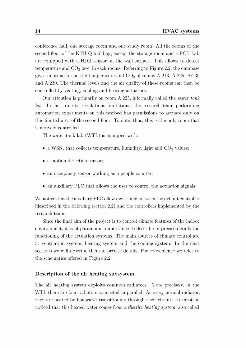
This map is shown in Figure 2.4.
What users can actively control is a valve placed before the first radiator and
whose opening percentages can be set through a SCADA web-based interface.
To help the development of controllers, the SCADA system accepts as inputs
percentage values that are directly percentages of the total amount of the
available heating power.
1This kind of systems distribute heat generated in a centralized location to residentialand commercial units. The heat is often obtained from cogeneration plants burning fossilfuels or biomasses (although heat-only boiler stations, geothermal heating and central solarheating are also used, as well as nuclear power). This generation mechanism is often used inNordic countries, specially because it allows heating conversions far from the city walls butalso because it uses both low quality heating sources and renewable energy sources.
16 HVAC systems
−20 −15 −10 −5 0 5 10 15 20
20
30
40
50
60
70
outside temperature []
tem
per
ature
ofth
ehot
wat
er[
]
Figure 2.4: Map showing the temperature of the water flowing through the radiators as afunction of the external temperature. The map represents reference temperatures, since it
neglects all the possible dynamics on these quantities.
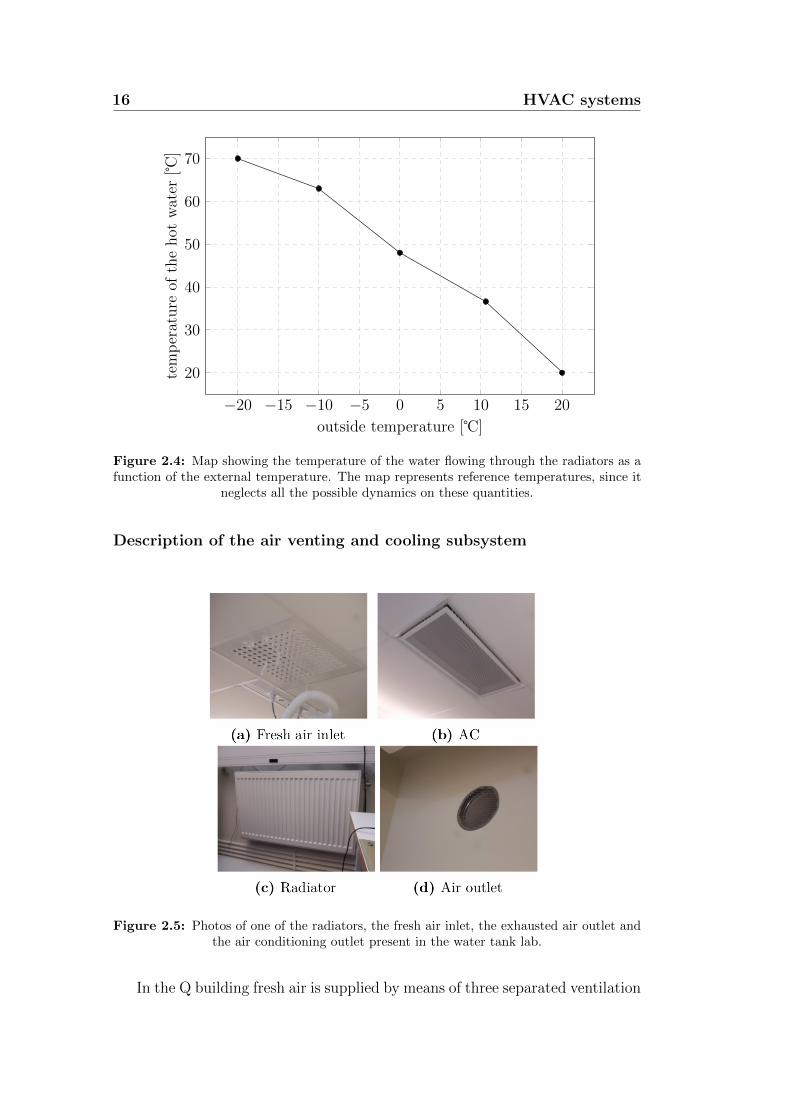
Description of the air venting and cooling subsystem
Figure 2.5: Photos of one of the radiators, the fresh air inlet, the exhausted air outlet andthe air conditioning outlet present in the water tank lab.
In the Q building fresh air is supplied by means of three separated ventilation
2.2 Peculiarities of the KTH HVAC Testbed 17
units. The fresh air flow for areas with special applications (like laboratories
or conference halls) is regulated by a Demand Controlled Ventilation (DCV),
while for floors housing office areas there is instead a constant fresh air flow. In
both these two cases venting is provided only in the day time and in a specific
time slot, specifically from 07:00 to 16:00.
In our particular case the venting and the cooling systems are actually
strictly connected. Indeed the air system comprises only one circuit that
provides fresh air to the venting and cooling system at a temperature that is
normally between 20 and 21 degrees, and that it is at the same pressure in the
whole duct. In more details the system composed by heat exchanger, pumps
and a heating/cooling system.
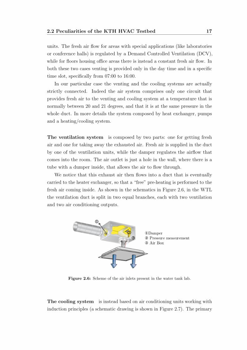
The ventilation system is composed by two parts: one for getting fresh
air and one for taking away the exhausted air. Fresh air is supplied in the duct
by one of the ventilation units, while the damper regulates the airflow that
comes into the room. The air outlet is just a hole in the wall, where there is a
tube with a dumper inside, that allows the air to flow through.
We notice that this exhaust air then flows into a duct that is eventually
carried to the heater exchanger, so that a “free” pre-heating is performed to the
fresh air coming inside. As shown in the schematics in Figure 2.6, in the WTL
the ventilation duct is split in two equal branches, each with two ventilation
and two air conditioning outputs.
Figure 2.6: Scheme of the air inlets present in the water tank lab.
The cooling system is instead based on air conditioning units working with
induction principles (a schematic drawing is shown in Figure 2.7). The primary
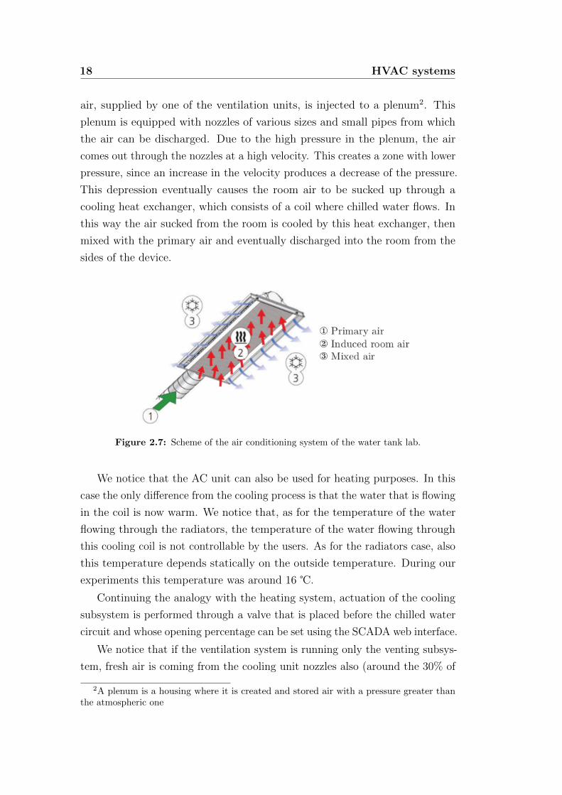
18 HVAC systems
air, supplied by one of the ventilation units, is injected to a plenum2. This
plenum is equipped with nozzles of various sizes and small pipes from which
the air can be discharged. Due to the high pressure in the plenum, the air
comes out through the nozzles at a high velocity. This creates a zone with lower
pressure, since an increase in the velocity produces a decrease of the pressure.
This depression eventually causes the room air to be sucked up through a
cooling heat exchanger, which consists of a coil where chilled water flows. In
this way the air sucked from the room is cooled by this heat exchanger, then
mixed with the primary air and eventually discharged into the room from the
sides of the device.
Figure 2.7: Scheme of the air conditioning system of the water tank lab.
We notice that the AC unit can also be used for heating purposes. In this
case the only difference from the cooling process is that the water that is flowing
in the coil is now warm. We notice that, as for the temperature of the water
flowing through the radiators, the temperature of the water flowing through
this cooling coil is not controllable by the users. As for the radiators case, also
this temperature depends statically on the outside temperature. During our
experiments this temperature was around 16 .
Continuing the analogy with the heating system, actuation of the cooling
subsystem is performed through a valve that is placed before the chilled water
circuit and whose opening percentage can be set using the SCADA web interface.
We notice that if the ventilation system is running only the venting subsys-
tem, fresh air is coming from the cooling unit nozzles also (around the 30% of
2A plenum is a housing where it is created and stored air with a pressure greater thanthe atmospheric one

2.2 Peculiarities of the KTH HVAC Testbed 19
the total amount of the available air flow). Vice-versa, when we want to cool
we need an air flow to chill. This leads us to notice the very important feature:
for the cooling system to be active we need the venting system to
be active. This implies that once the cooling system is running
the venting system is also running, and thus we must expect a
air flow at around 20 from the venting nozzles.
Effects of the ventilation on the cooling/heating as described before,
the ventilation system affects both the heating and cooling processes. Figure 2.8
shows the entire air process in the schematic version that the user finds on the
SCADA web interface. The previous processes can be summarized as follows:
1. the fresh air from outside is imported through a valve (denoted with the
code ST201);
2. the air is then is filtered by opportune air filters;
3. after that the air is processed by an heater exchanger which exploits the
heat of exhaust air flow. As shown in the Figure 2.8 the imported fresh
air is warmed up to 19.4;
4. the pump TF001 then pushes the warmed air to the heating and cooling
system sequentially; due to this the temperature of the fresh air that
flows through the ducts is around 20 in each room;
5. the fresh air is eventually discharged into the rooms at a temperature
that is always around 20.
Summarizing, when the temperature of the room is below 20 the air from
the ventilation helps the heating system to increase the indoor temperature.
Otherwise, if the temperature is greater then 20the ventilation system helps
to lower the room temperature.
Soft PLCs and the default controller
For completeness we now describe what is the current practice.
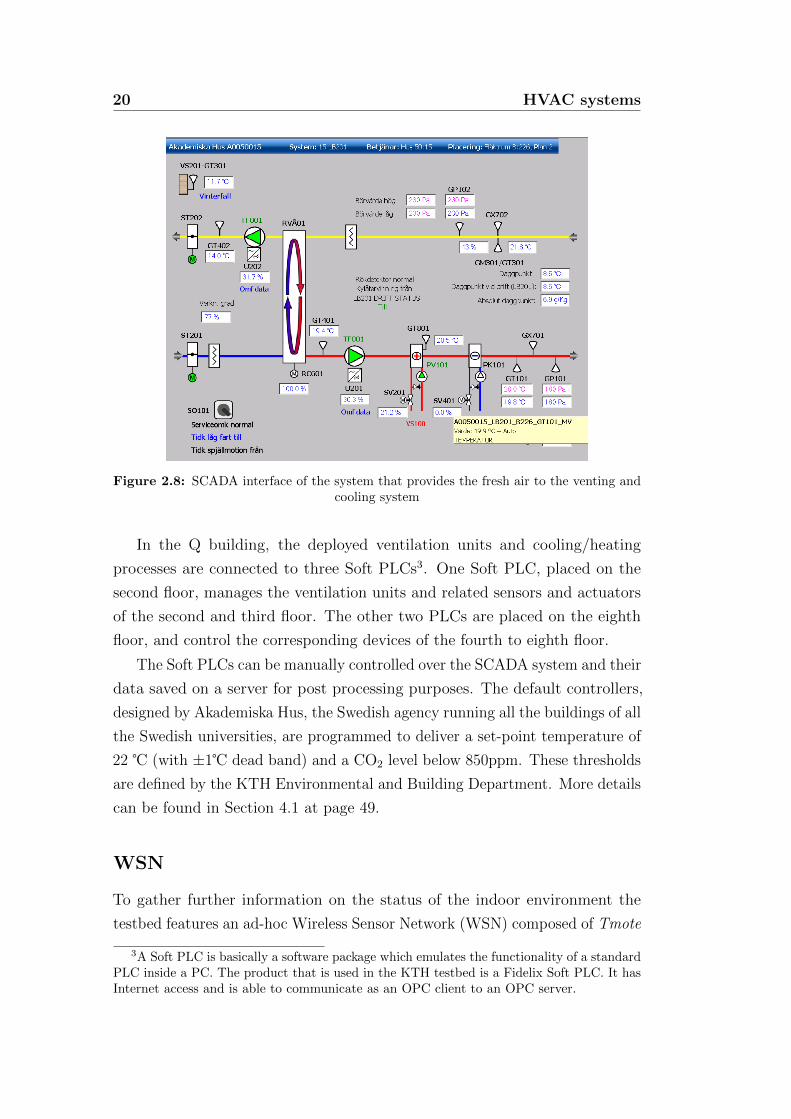
20 HVAC systems
Figure 2.8: SCADA interface of the system that provides the fresh air to the venting andcooling system
In the Q building, the deployed ventilation units and cooling/heating
processes are connected to three Soft PLCs3. One Soft PLC, placed on the
second floor, manages the ventilation units and related sensors and actuators
of the second and third floor. The other two PLCs are placed on the eighth
floor, and control the corresponding devices of the fourth to eighth floor.
The Soft PLCs can be manually controlled over the SCADA system and their
data saved on a server for post processing purposes. The default controllers,
designed by Akademiska Hus, the Swedish agency running all the buildings of all
the Swedish universities, are programmed to deliver a set-point temperature of
22 (with ±1 dead band) and a CO2 level below 850ppm. These thresholds
are defined by the KTH Environmental and Building Department. More details
can be found in Section 4.1 at page 49.
WSN
To gather further information on the status of the indoor environment the
testbed features an ad-hoc Wireless Sensor Network (WSN) composed of Tmote
3A Soft PLC is basically a software package which emulates the functionality of a standardPLC inside a PC. The product that is used in the KTH testbed is a Fidelix Soft PLC. It hasInternet access and is able to communicate as an OPC client to an OPC server.

2.2 Peculiarities of the KTH HVAC Testbed 21
Sky nodes. These Tmote Sky devices include a number of on-board sensors to
measure light, temperature and humidity. In addition of that, other external
sensors may be connected to the motes, using the dedicated ADC channel on
the opportune expansion area.
In particular some motes are equipped with an additional CO2 and temper-
ature sensor (this has been done specially to avoid alterations in the measured
temperatures induced by the heat that the motes microprocessor release, and
also to to reach places that could not be accessible in other ways).
Figure 2.9: A Tmote Sky with highlighted the various measurements systems.
The WTL currently comprises 10 motes in the WTL, 4 motes in the rooms
beside, 1 in the corridor and 1 outside the building. The nodes form a star
network, and send data to a root mote directly connected with a server collecting
and storing all the information (see Figure 2.11).
The motes forwards the sensed data to the main server every 30 seconds.
The list of the nodes and of their main features are summarized in Table 2.1.
People counter
To measure the room occupancy the testbed features a tailored people counter,
mounted over the entrance of the WTL. The counter is a thermal based camera
commercialized by IRISYS and composed by two modules: the dual view IP
and the node IP master.
The node IP master IRC3000 [35] is a people counting devices with the
imaging optics, sensor, signal processing and interfacing electronics all contained
22 HVAC systems
Figure 2.10: Tipical star network topology, it is used also in our network
Root 1
2
3
20
5
6
7 8 9
109
110
111
213
4
12
11
1
36
38 37 35
39
Figure 2.11: Map of the sensors deployed in the KTH testbed

2.2 Peculiarities of the KTH HVAC Testbed 23
Mote Id Spot T H C L Description
1000 WTL - - - - Root1001 WTL
√ √ √- Exhaust air outlet
1002 WTL√ √
- - Environment1003 Corridor
√ √- - Corridor
1004 WTL√ √ √
- Fresh air inlet1005 WTL
√ √- - Room wall temperature
1006 Outside√ √
- - Outdoor wall temperature1007 WTL
√ √- - Room wall temperature
1008 WTL√
- - - Surface of radiator hot water inlet1009 WTL
√- - - Surface of radiator hot water outlet
1011 WTL√ √
- - Room wall temperature1012 WTL
√ √- - Air conditioning outlet
1020 WTL - - -√
Environment1035 WTL
√ √- - Environment
1036 WTL√ √
- - Room wall temperature1037 WTL
√ √- - Ceiling
1038 WTL√ √
- - Floor1039 3rd Floor
√ √- - Floor
1109 PCB Lab√ √
- - Beside room environment1110 PCB Lab
√ √- - Beside room environment
1111 PCB Lab√ √
- - Beside room environment1213 Storage room
√ √- - Beside room environment
Table 2.1: Summary of the mote of the WSN (T, H, C, L stand for temperature, humidity,CO2 and light respectively)
24 HVAC systems
within a molded plastic housing. The unit is used in a downward looking manner,
as the unit functions optically recognize the heat emitted by people passing
underneath as infrared radiation, collected through a germanium lens with
a 60’ field of view. The sensing area is a square on the floor whose width is
approximately equal to the mounting height.
The dual view IP IRC3030 [36] multiplexes both the thermal people count
data, the stored count data, diagnostic information and the video stream into a
single IP data stream. The IP capability allows remote viewing, configuration
and data collection over IP infrastructure, either over an in-store LAN, or for
worldwide viewing from remote locations over the Internet.
Figure 2.12: The people counting devices: left, the IRC3030 device. Right, the IRC3000.
Programmable Logic Controller (PLC)
In addition to the soft PLC the testbed comprises an additional PLC, a Fidelix
FX-2025A [37], that allows to communicate and actuate. The device is endowed
with a freely programmable web server, based on an industrial PC running
a Windows CE operating system. The device accesses to all the data of the
Akademiska Hus central system and can send command to the actuation devices.
Moreover it is also connected to the dedicated temperature, CO2 and binary
motion sensors present in the testbed.
Weather forecasts
As highlighted in our literature review, the knowledge of the future outdoor
conditions is crucial for achieving good control performance in terms of energy
savings. To this aim the testbed server fetches and stores information the web
site www.wunderground.com. More precisely, the available data are:

2.2 Peculiarities of the KTH HVAC Testbed 25
• temperature (current and the hourly forecasts for the next 72 hours);
• wind speed (current and the hourly forecasts for the next 72 hours);
• wind direction (current and the hourly forecasts for the next 72 hours);
• wind gusts (only the current status);
• precipitation (current and the hourly forecasts for the next 72 hours);
• external air pressure (only the current status).
Central PC and LabVIEW
The pulsing heart of the testbed is located in a dedicated server running in
the WTL. This server implements all the logic that allows the user to perform
all the possible communications with the various devices. The instruments
that make these communications possible have been designed and developed
in LabVIEW. The server is connected through Ethernet cables to the KTH
network and to the external PLC, and is reachable through dedicated TCP-IP
Internet ports. A schematic representation of the whole communication system
is shown in Figure 2.13.
Figure 2.13: A scheme representing the whole testbed system; LabVIEW is the tool thatallow the user to communicate with the whole network by a collection of virtual instruments.
PLC virtual instrument the server continuously runs an OPC Server that
listens data coming from the dedicated PLC. In the meantime, an OPC Client
runs on a virtual instrument and processes this data from the PLC. Eventually,
this information is sent to the dedicated database.
26 HVAC systems
People counter and weather virtual instruments the information com-
ing from the people counter is processed by a dedicated virtual instrument,
people counter.vi, that reads the counted value of the device every four sec-
onds and sends it to the virtual instrument managing the database. A similar
procedure is implemented to manage the weather forecasts, weather.vi.
Motes virtual instrument the root of the dedicated WSN is mounted on
one of the USB ports of the server. Through a serial forwarding, the data from
this root wireless node are then processed by a dedicated virtual instrument,
mote.vi, that sends in turn these data to the database virtual instrument.
Database and control virtual instruments all the data coming from the
previous virtual instruments are received by an additional virtual instrument,
database.vi, that writes them into a database. This instrument sends also
these real-time data to another virtual instrument, control.vi, that enables
users to have remote access to the sensed data and it also allows the actuation.
We notice that user can have access to this information only through an
appropriate client and credentials.
Remote access
As already written in the previous sections, all the sensed information is
stored into a database. The central server also runs an Apache Web Server
that allows the access to this database through the dedicated web page http:
//hvac.ee.kth.se/. With a simple web interface, shown in Figure 2.14, it is
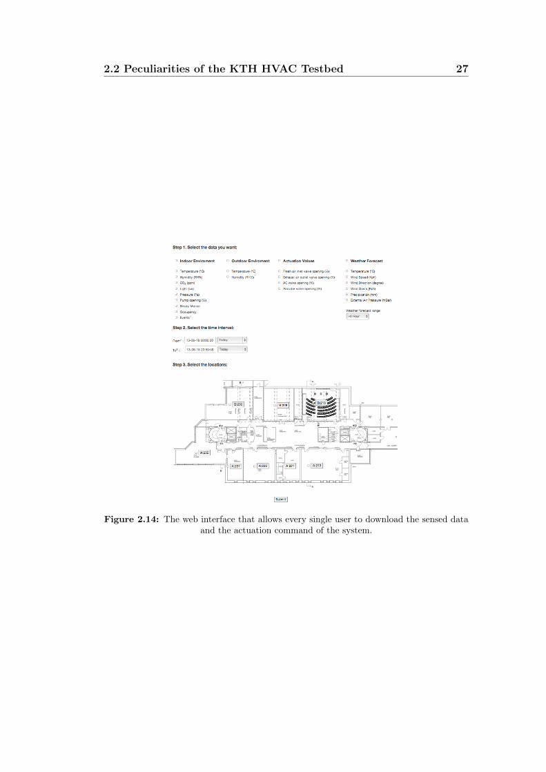
possible to download information about the system in a handy .txt file.
Accessing the data and giving actuation commands is possible by using some
other virtual instruments, like ControlConnectToHVAC.vi or ControlGetDataPlcs.vi4.
These instruments thus allow every user with LabVIEW to potentially actuate
remotely the system. Some of these instruments have also been implemented
in Matlab, so that users can run control algorithms remotely.
4The complete list can be found on https://code.google.com/p/kth-hvac/wiki/
RemoteAccess#Creating_connection_to_HVAC_system with more explanations on how touse them, and also with the possibility of downloading them.
2.2 Peculiarities of the KTH HVAC Testbed 27
Figure 2.14: The web interface that allows every single user to download the sensed dataand the actuation command of the system.

28 HVAC systems
3Building model and System
identification
3.1 Physics-based model
Model based control paradigms need a mathematical description of the system
of interest. For this reason, in this chapter we shall deal with the derivation of
a proper model which accurately describes the dynamics of the signals involved
in the system. In particular, aiming at controlling the comfort features, we
are interested in the behaviour of two physical characteristics, which are the
temperature of the room and the concentration of CO2. In this work, we shall
not focus on humidity, due to the fact that in the testbed there is no device
capable of modifying its evolution (i.e. there is no dehumidifier or similar
devices). In order to describe the mentioned quantities, we adopted a physical
modeling of the whole system (white-box approach), using as reference [32]. In
such work, authors derive models that try to explain the system using relatively
simple relations, still keeping a good degree of accuracy (i.e. such that the
system is well described). In this way, the computational burden of the model
remains low, according to the needs of MPC controllers. These models are
30 Building model and System identification
built under the following assumptions:
• no infiltrations are considered, so that the inlet airflow in the zone equals
the outlet airflow;
• the zone is well mixed, i.e. the temperature and the concentration of CO2
are constant with respect to the space and do not depend on the place
they are measured;
• the thermal effects of the vapor production are neglected.
All the parameters involved in this subsection are described in Table 3.1
Room temperature model
As in [32], the room temperature is computed via the following energy balance
of the zone, modeled as a lumped node.
mair,zonecpadTroom
dt= Qvent +Qcool +Qheat +Qint +
∑jQwall,j +
∑jQwin,j.
(3.1)
In (3.1), the left-hand term represents the heat stored in the air within the
room. Qvent is the heat flow due to ventilation, Qcool and Qheat are the heating
and cooling flows. These are necessary in order to keep the room environment
within thermally comfortable conditions. The quantity Qint incorporates the
internal gains, which are given by the sum of the heat flows due to occupancy,
equipment and lighting. Qwall,j and Qwin,j represent the heat flows exchanged
between walls and room and windows and room respectively. Each term of the
Equation (3.1) is:
Qvent = mventcpa∆Tvent = mventcpa
(Tai − Troom
),
Qcool = mcoolcpa∆Tcool = mcoolcpa
(Tsa − Troom
),
Qheat = Aradhrad∆Trad = Aradhrad
(Tmr − Troom
),
Qint = cNpeople,
Qwall,j = hiAjwall
(T j
wall,i − Troom
),
Qwin,j =
(Tamb − Troom
)Rj
win
+GjAjwinI
j.
(3.2)
3.1 Physics-based model 31
From (3.1) and (3.2) we obtain the differential equation
dTroom
dt=
mvent
(Tai − Troom
)mair,zone
+mcool
(Tsa − Troom
)mair,zone
+Aradhrad
(Tmr − Troom
)mair,zonecpa
+cNpeople
mair,zonecpa
+∑
j
hiAjwall
(T j
wall,i − Troom
)mair,zonecpa
+∑
j
(Tamb − Troom
)Rj
winmair,zonecpa
+
∑jG
jAjwinI
j
mair,zonecpa
(3.3)
In order to have the whole description of the temperature dynamics, we also
need to model the behavior of the indoor wall temperature, say T jwall,i, of
each surface. These temperature signals are calculated by means of an energy
balance between the outdoor and indoor surfaces. All the walls are modeled as
a “two capacitance and three resistance” systems (2C3R), where the thermal
capacity, denoted by C j, is determined using the Active Heat Capacity model
proposed by [38]. A representation of such a model is shown in Figure 3.1;
solving the circuit we can find in/out relationships for wall temperatures. More
precisely, such relationships are
dT jwall,o
dt=
[hoA
jwall
(T j
ee − Tjwall,o
)+
(T j
wall,i − Tjwall,o
)Rj
wall
]C j/2
(3.4)
dT jwall,i
dt=
[hiA
jwall
(Troom − T j
wall,i
)+
(T j
wall,o − Tjwall,i
)Rj
wall
]C j/2
(3.5)
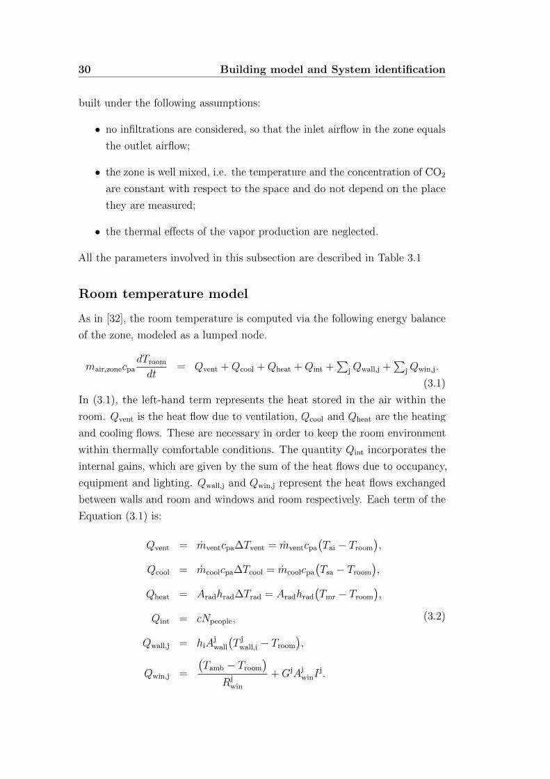
The equivalent external temperature T jee accounts for the different radiation
heat exchange due to the orientation of the external walls. The outdoor
temperature is modified by the effects of radiation on the j-th wall.
Tee,j = Tamb +aI j
αe
. (3.6)
All the values of the parameters were determined by means of evaluations based
on the geometry of the building, the manufacturing materials and the knowledge
32 Building model and System identification
TT T Troomwall,owall,i
ee
1h0
1hi
Rwallj
jj j
C Cj j
Figure 3.1: Electric scheme of the model of the walls. The three resistances 1/ho, Rjwall
and 1/hi are placed between the equivalent temperature T jee, and the temperatures T j
wall,o,
T jwall,i and Troom. Rj
wall [°C/W] and Cj [J/°C] are the thermal resistance and the thermalcapacity of the j-th wall respectively
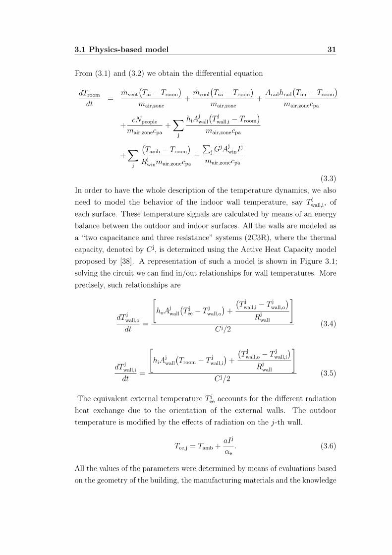
of the construction standards. The resulting model was validated to be in
accordance with the Stockholm climate. Its outcomes were compared with the
predicted values given by simulations carried out in IDA [39], which represents
one of the most effective softwares for building model simulations. The data
regarding the climate conditions were taken from the Swedish Meteorological
and Hydrological Institute (SMHI). The comparison was performed under the
same conditions of ventilation, solar radiation, internal gains and occupancy. In
both cases, thermal bridges and infiltrations were neglected. In order to clearly
display the effects of the thermal behavior of the room model, no heating and
cooling systems were simulated. The results are depicted in Figure 3.10.
0 20 40 60 80 100 120 140 160 18024
25
26
27
28
time [h]
tem
per
ature
[]
tMatlab
tIDA
Figure 3.2: Validation of the model performed with the software IDA ICE.
In Figure 3.3 a comparison between the simulation of the model using real

3.1 Physics-based model 33
inputs and the measured temperature of the room is shown. Unfortunately, it
20:00 04:00 12:00 20:00 04:00 12:0020.2
20.4
20.6
20.8
21
21.2
time
tem
per
ature
[]
measuredsimulated
Figure 3.3: Comparison between the simulated temperatures obtained with the physicalmodel and the actual measured room temperature.
appears that the model is not able to fit adequately with the measured data.
However, it may be good for capturing long period trends. The faster dynamics
of the room temperature are not properly followed by our model. Nevertheless,
we shall make use of this model, since we assessed that its accuracy is good
enough for our purposes.
CO2 concentration model
As in [32], the CO2 concentration model is determined by a balance between
the amount of CO2 that is flowing inside the room Cin, the amount flowing
outside1 because of the air outlet pump Cout, and the amount of CO2 that is
generated by the occupants Cocc. More precisely, assuming no leakages, i.e. no
spontaneous outflowing of air, this balance leads to
VdCCO2
dt= Cin − Cout + Cocc. (3.7)
where
1We made the reasonable assumption that the air flowing out of the room has the sameconcentration CO2 of the air inside the room

34 Building model and System identification
Cin = mairCCO2,i,
Cout = mairCCO2 ,
Cocc = gCO2Npeople,
(3.8)
From (3.7) and (3.8) we obtain the differential equation
dCCO2
dt=mairCCO2,i
V− mairCCO2
V+gCO2Npeople
V. (3.9)
The derived model was then discretized by using the Euler backward method,
which yields (the sampling time is neglected for simplicity)
CCO2(t+ 1) = CCO2(t) + mair(CCO2(t)− CCO2,i) + gCO2Npeople(t). (3.10)
We assessed that this model could not describe the CO2 behaviour accurately
enough. Its main drawback is given by the fact that no zero decaying happens
if the system is not excited. In this way, all the unavoidable errors accumulate,
making the model outcomes differ substantially from the real behavior. An
example of this is in Figure 3.4. For this reason, we decided to identify a new
0 400 800 1,200 1,600 2,000
−200
0
200
400
600
time [min]
CO
2co
nce
ntr
atio
n[p
pm
]
realphysical model
Figure 3.4: Validation of the CO2 physical model.
model using the well-known Prediction Error Method (PEM) identification
technique [40]. The model order was established according to the knowledge
of the physical model obtained before. In this sense, a grey-box modeling
approach was adopted. Furthermore, adopting simple models permits to obtain
3.1 Physics-based model 35
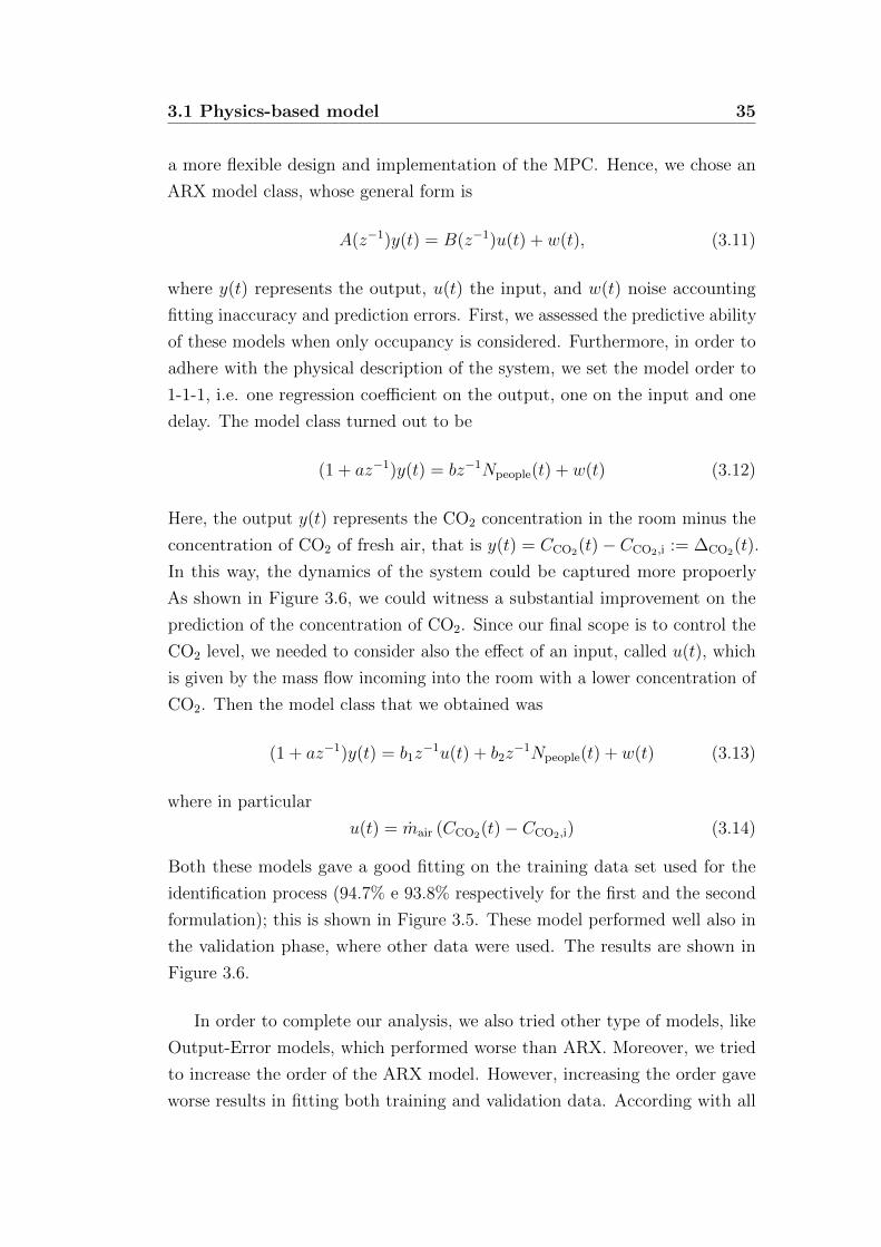
a more flexible design and implementation of the MPC. Hence, we chose an
ARX model class, whose general form is
A(z−1)y(t) = B(z−1)u(t) + w(t), (3.11)
where y(t) represents the output, u(t) the input, and w(t) noise accounting
fitting inaccuracy and prediction errors. First, we assessed the predictive ability
of these models when only occupancy is considered. Furthermore, in order to
adhere with the physical description of the system, we set the model order to
1-1-1, i.e. one regression coefficient on the output, one on the input and one
delay. The model class turned out to be
(1 + az−1)y(t) = bz−1Npeople(t) + w(t) (3.12)
Here, the output y(t) represents the CO2 concentration in the room minus the
concentration of CO2 of fresh air, that is y(t) = CCO2(t)− CCO2,i := ∆CO2(t).
In this way, the dynamics of the system could be captured more propoerly
As shown in Figure 3.6, we could witness a substantial improvement on the
prediction of the concentration of CO2. Since our final scope is to control the
CO2 level, we needed to consider also the effect of an input, called u(t), which
is given by the mass flow incoming into the room with a lower concentration of
CO2. Then the model class that we obtained was
(1 + az−1)y(t) = b1z−1u(t) + b2z
−1Npeople(t) + w(t) (3.13)
where in particular
u(t) = mair (CCO2(t)− CCO2,i) (3.14)
Both these models gave a good fitting on the training data set used for the
identification process (94.7% e 93.8% respectively for the first and the second
formulation); this is shown in Figure 3.5. These model performed well also in
the validation phase, where other data were used. The results are shown in
Figure 3.6.
In order to complete our analysis, we also tried other type of models, like
Output-Error models, which performed worse than ARX. Moreover, we tried
to increase the order of the ARX model. However, increasing the order gave
worse results in fitting both training and validation data. According with all
36 Building model and System identification
0 1,000 2,000 3,000 4,000 5,000380
400
420
440
460
480
500
520
540
560
580
600
time [min]
CO
2co
nce
ntr
atio
n[p
pm
]realoccupancyoccupancy & u(t)
Figure 3.5: Fitting of the CO2 models with the validation set of data.
0 400 800 1,200 1,600 2,000
400
450
500
550
600
time [min]
CO
2co
nce
ntr
atio
n[p
pm
]
realoccupancyoccupancy & u(t)
Figure 3.6: Validation of the CO2 models.
3.1 Physics-based model 37
these considerations, the final model for describing the CO2 concentration is
then an ARX111 that accounts for both occupancy and input u(t) of (3.14).
A reasonable sample time of the discrete model was 10′. Hence, our adopted
model is
∆CO2(t) = +0.9343 ·∆CO2(t−1)−0.1255 ·u(t−1)+8.9129 ·Npeople(t−1)+w(t)
(3.15)
Note that now, when no inputs are given, i.e. no people are in the room and
no fresh air is injected, the concentration of CO2 tends to set to its fresh-air
value CCO2,i. This can be explained by the fact that assuming no leakages in
the room is indeed a strong assumption that does not hold in the true system.
Variable U.M. Description
αe [W/m2°C] external heat transfer coefficienta [−] absorption factor for shortwave radiation
Arad [m2] emission area of the radiators
Ajwall [m2] wall area on the j-th surface
Ajwin [m2] area of the window on the j-th surfacec [W ] constant related to equipment and occupants activity
CCO2,i [ppmV] inlet air CO2 concentrationCCO2 [ppmV] concentration of CO2 within the roomcpa [J/kg°C] specific heat of the dry airgCO2 [m3
CO2/pers.] generation rate of CO2 per person
Gj [−] G-value (SHGC) of the window on the j-th surfacehi [W/m2°C] indoor heat transfer coefficientho [W/m2°C] outdoor heat transfer coefficienthrad [W/m2°C] heat transfer coefficient of the radiatorsI j [W/m2] solar radiation on the j-th surface
mair,zone [kg] air mass in the roommcool [kg/s] mass flow through the cooling branchmvent [kg/s] mass flow through the ventilation branchNpeople [−] number of occupants in the room
Rjwin [°C/W] thermal resistance of the window on the j-th surfaceTai [°C] air inlet temperature, from the venting outletTsa [°C] supply air temperature, from the cooling outletTamb [°C] outdoor temperature
T jwall,i [°C] indoor surface temperature of the wall on the j-th surface
Tmr [°C] mean radiant temperature of the radiatorsV [m3] volume of the air inside the room
Table 3.1: Summary of the parameters involved in the building model.
38 Building model and System identification
3.2 Devices to be identified
As shown in the previous section, in order to control our outputs we need a
description of some physical features and their connections with our actuation
signals. Our actuation on the cooling, venting and heating dumpers (or valves)
must be given in terms of percentages. However, we are not aware of the
behavior of the physical response of the system. For this reason, we need to
test such a behavior.
More precisely, we aim at finding the following features.
• Heating: link the Tmr to the valve opening percentage of the radiator.
• Venting: link mair, mvent and mcool to the dampers opening percentage of
the venting (inlet and outlet).
• Cooling: find a relationship between Tsa and the the valve opening
percentage of the cooling.
In the next subsection we present all the tests performed on the testbed.
Test on the average radiant temperature
The first test was made in order to link the mean radiant temperature of the
radiators, Tmr, and the radiator opening valve percentage. Unfortunately, we
could run one test only. This because of a problem with the change of the
outdoor weather conditions, which made the main system detect a change from
“winter” to “summer”. This interrupted the water flow to the radiator (closing
the main valve) and, as shown on Figure 2.5, the water passing through them
did not affect the heating of the room. Thanks to Akademiska Hus, we could
run one test using water at 46 2.
We designed a test based on inputs shaped as stairs with steps of size of
20%, each one every 10′, from 0% to 100% and then back to 0%. To evaluate
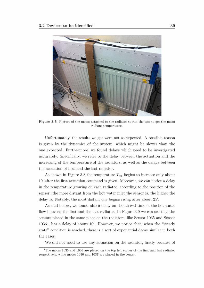
the temperature Tmr, we put some sensors on the radiators, precisely on the
first one and on the last one of the cascade.
We took the mean radiant temperature as the mean of the temperature
of these sensors. We also assessed whether a mote positioned in the middle
radiator could give the same description with good approximation. An example
of sensor placement is in Figure 3.7
2Of course more precise and deep investigations must be done during the winter period
3.2 Devices to be identified 39
Figure 3.7: Picture of the motes attached to the radiator to run the test to get the meanradiant temperature.
Unfortunately, the results we got were not as expected. A possible reason
is given by the dynamics of the system, which might be slower than the
one expected. Furthermore, we found delays which need to be investigated
accurately. Specifically, we refer to the delay between the actuation and the
increasing of the temperature of the radiators, as well as the delays between
the actuation of first and the last radiator.
As shown in Figure 3.8 the temperature Tmr begins to increase only about
10′ after the first actuation command is given. Moreover, we can notice a delay
in the temperature growing on each radiator, according to the position of the
sensor: the more distant from the hot water inlet the sensor is, the higher the
delay is. Notably, the most distant one begins rising after about 25′.
As said before, we found also a delay on the arrival time of the hot water
flow between the first and the last radiator. In Figure 3.9 we can see that the
sensors placed in the same place on the radiators, like Sensor 1035 and Sensor
10363, has a delay of about 10′. However, we notice that, when the “steady
state” condition is reached, there is a sort of exponential decay similar in both
the cases.
We did not need to use any actuation on the radiator, firstly because of
3The motes 1035 and 1036 are placed on the top left corner of the first and last radiatorrespectively, while motes 1030 and 1037 are placed in the center.
40 Building model and System identification
0 20 40 60 80 100 1200
10
20
30
40
50
60
70
80
90
100
time [min]
per
centa
ge
Heating
20
22
24
26
28
30
32
34
36
38
40
Tem
per
ature
[]
10321035103010331034Tmr
Figure 3.8: Test on the radiators: first radiator temperature response. The motes areplaced on the radiator in this order: 1032 on the top right, where there is the hot waterinlet,1035 on the top left, 1030 in the center, 1034 on the bottom left and 1033 on the bottom
right, where there is the hot water outlet.
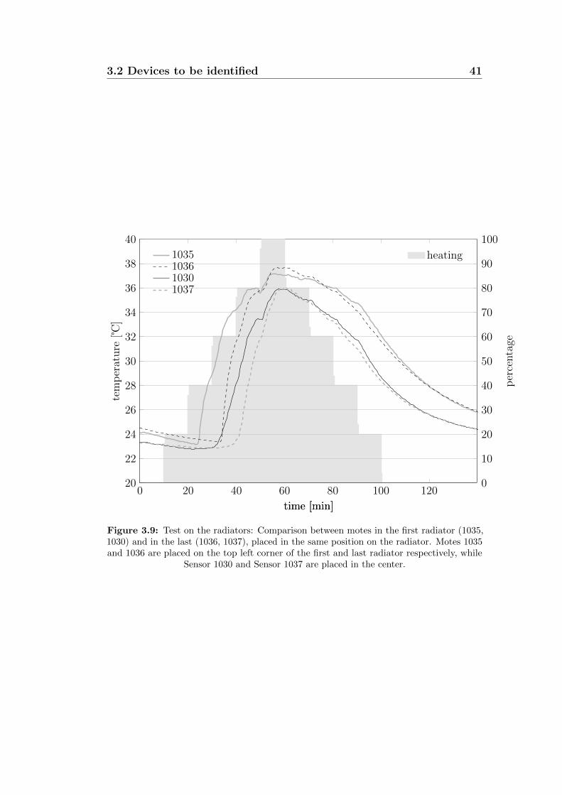
3.2 Devices to be identified 41
0 20 40 60 80 100 1200
10
20
30
40
50
60
70
80
90
100
time [min]p
erce
nta
ge
heating
20
22
24
26
28
30
32
34
36
38
40
time [min]
tem
per
ature
[]
1035103610301037
Figure 3.9: Test on the radiators: Comparison between motes in the first radiator (1035,1030) and in the last (1036, 1037), placed in the same position on the radiator. Motes 1035and 1036 are placed on the top left corner of the first and last radiator respectively, while
Sensor 1030 and Sensor 1037 are placed in the center.
42 Building model and System identification
the impossibility of getting hot water during the tests, secondly because we
were running our tests during the summer time. What we had to employ
was an empirical characterization of the actuation command, considering the
temperature of the hot water. However, for our final goal this was insufficient,
thus the first step must be repeated for obtaining an improvement.
Test on the air inlet mass flow
In this subsection we seek for a relation between the opening valve percentage
of the dumper of the ventilation system (Av(t)) and the air mass flow actually
carried into the room (mair(t)).
Our understanding of the ventilation system control design leads us to
deduce that this relation has to be approximately linear. A linear-quadratic
relation with a small coefficient on the quadratic term is also considered.
As explained in Section 2.2 the ventilation duct that comes in the testbed
is split in two equal branches with the same characteristics, and accordingly
with the same air mass flow4. Both the branches are in turn split in two parts:
one part for the cooling system and one for the ventilation. Thus, we can write
mair(t) = mvent(t) + mcool(t) (3.16)
where mvent(t) is the part of air mass flow for the ventilation system and mcool(t)
is the one for the cooling system.
We decided to measure the air mass flow (both in the cooling duct and
the venting duct) at four different percentages of valve opening (30%, 50%,
70% and 100%). We attempted to build a map assuming that there is no
dynamic features behind, i.e. the opening of the valve reaches immediately the
corresponding air mass flow5.
These measurements were made, thanks to the support of a technician,
using an anemometer. We measured the average air velocity (vair[ms
]), by
4It seems reasonable, due to the symmetric geometry of the system and the operatingconditions of the ventilation system, to assume that the branches are specular. The measure-ments have then been carried out only on one branch. According to the previous assumptions,the total air flow is twice the air flows in the measured branch
5This assumption has been done because the time constant to reach the steady statevalues are considerably small compared to the other time constants of the system
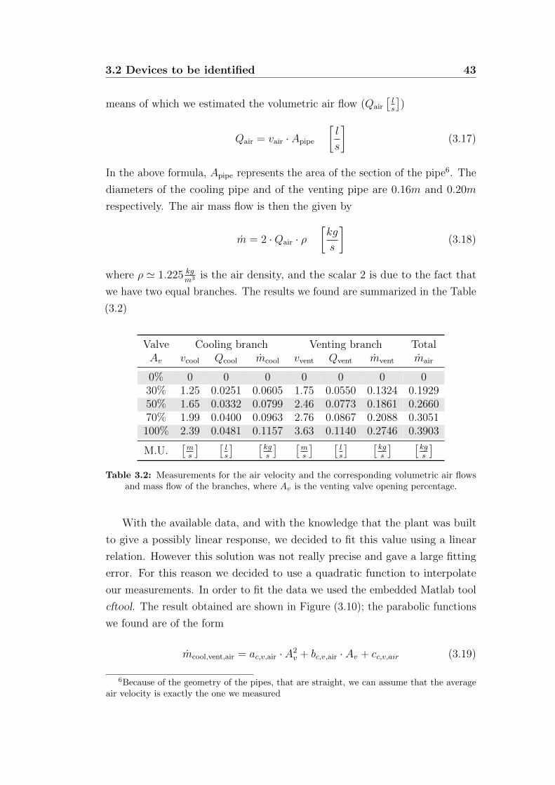
3.2 Devices to be identified 43
means of which we estimated the volumetric air flow (Qair
[ls
])
Qair = vair · Apipe
[l
s
](3.17)
In the above formula, Apipe represents the area of the section of the pipe6. The
diameters of the cooling pipe and of the venting pipe are 0.16m and 0.20m
respectively. The air mass flow is then the given by
m = 2 ·Qair · ρ[kg
s
](3.18)
where ρ ' 1.225 kgm3 is the air density, and the scalar 2 is due to the fact that
we have two equal branches. The results we found are summarized in the Table
(3.2)
Valve Cooling branch Venting branch TotalAv vcool Qcool mcool vvent Qvent mvent mair
0% 0 0 0 0 0 0 030% 1.25 0.0251 0.0605 1.75 0.0550 0.1324 0.192950% 1.65 0.0332 0.0799 2.46 0.0773 0.1861 0.266070% 1.99 0.0400 0.0963 2.76 0.0867 0.2088 0.3051100% 2.39 0.0481 0.1157 3.63 0.1140 0.2746 0.3903
M.U.[ms
] [ls
] [kgs
] [ms
] [ls
] [kgs
] [kgs
]Table 3.2: Measurements for the air velocity and the corresponding volumetric air flows
and mass flow of the branches, where Av is the venting valve opening percentage.
With the available data, and with the knowledge that the plant was built
to give a possibly linear response, we decided to fit this value using a linear
relation. However this solution was not really precise and gave a large fitting
error. For this reason we decided to use a quadratic function to interpolate
our measurements. In order to fit the data we used the embedded Matlab tool
cftool. The result obtained are shown in Figure (3.10); the parabolic functions
we found are of the form
mcool,vent,air = ac,v,air · A2v + bc,v,air · Av + cc,v,air (3.19)
6Because of the geometry of the pipes, that are straight, we can assume that the averageair velocity is exactly the one we measured
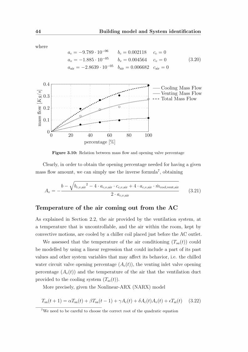
44 Building model and System identification
whereac = −9.789 · 10−06 bc = 0.002118 cc = 0
av = −1.885 · 10−05 bv = 0.004564 cv = 0
aair = −2.8639 · 10−05 bair = 0.006682 cair = 0
(3.20)
0 20 40 60 80 1000
0.1
0.2
0.3
0.4
percentage [%]
mas
sflow
[Kg/s
] Cooling Mass FlowVenting Mass FlowTotal Mass Flow
Figure 3.10: Relation between mass flow and opening valve percentage
Clearly, in order to obtain the opening percentage needed for having a given
mass flow amount, we can simply use the inverse formula7, obtaining
Av = −b−
√bc,v,air
2 − 4 · ac,v,air · cc,v,air + 4 · ac,v,air · mcool,vent,air
2 · ac,v,air
(3.21)
Temperature of the air coming out from the AC
As explained in Section 2.2, the air provided by the ventilation system, at
a temperature that is uncontrollable, and the air within the room, kept by
convective motions, are cooled by a chiller coil placed just before the AC outlet.
We assessed that the temperature of the air conditioning (Tsa(t)) could
be modelled by using a linear regression that could include a part of its past
values and other system variables that may affect its behavior, i.e. the chilled
water circuit valve opening percentage (Ac(t)), the venting inlet valve opening
percentage (Av(t)) and the temperature of the air that the ventilation duct
provided to the cooling system (Tai(t)).
More precisely, given the Nonlinear-ARX (NARX) model
Tsa(t+ 1) = αTsa(t) + βTsa(t− 1) + γAc(t) + δAc(t)Av(t) + εTai(t) (3.22)
7We need to be careful to choose the correct root of the quadratic equation
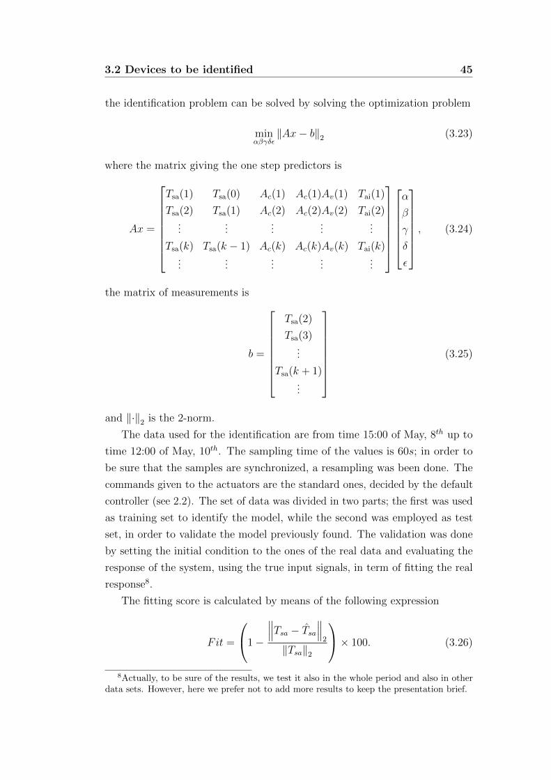
3.2 Devices to be identified 45
the identification problem can be solved by solving the optimization problem
minαβγδε
‖Ax− b‖2 (3.23)
where the matrix giving the one step predictors is
Ax =
Tsa(1) Tsa(0) Ac(1) Ac(1)Av(1) Tai(1)
Tsa(2) Tsa(1) Ac(2) Ac(2)Av(2) Tai(2)...
......
......
Tsa(k) Tsa(k − 1) Ac(k) Ac(k)Av(k) Tai(k)...
......
......
α
β
γ
δ
ε
, (3.24)
the matrix of measurements is
b =
Tsa(2)
Tsa(3)...
Tsa(k + 1)...
(3.25)
and ‖·‖2 is the 2-norm.
The data used for the identification are from time 15:00 of May, 8th up to
time 12:00 of May, 10th. The sampling time of the values is 60s; in order to
be sure that the samples are synchronized, a resampling was been done. The
commands given to the actuators are the standard ones, decided by the default
controller (see 2.2). The set of data was divided in two parts; the first was used
as training set to identify the model, while the second was employed as test
set, in order to validate the model previously found. The validation was done
by setting the initial condition to the ones of the real data and evaluating the
response of the system, using the true input signals, in term of fitting the real
response8.
The fitting score is calculated by means of the following expression
Fit =
1−
∥∥∥Tsa − Tsa∥∥∥2
‖Tsa‖2
× 100. (3.26)
8Actually, to be sure of the results, we test it also in the whole period and also in otherdata sets. However, here we prefer not to add more results to keep the presentation brief.
46 Building model and System identification
Furthermore, in order to obtain more accurate scores we also evaluated the
index
Fitm =
1−
∥∥∥(Tsa − Tsa)− (Tsa − ¯Tsa)
∥∥∥2∥∥Tsa − Tsa∥∥2
× 100 (3.27)
where Tsa is the vector with the real response of the system, whose mean is Tsa,
and Tsa is the vector with the response of the identified system, whose mean is¯Tsa.
The parameters that were found are
α = 1.4250 β = −0.4564 γ = −1.5590 · 10−3 δ = 8.8073 · 10−6 ε = 0.0303
(3.28)
With these parameters the fitting score were
Fit = 98% Fitm = 73% (3.29)
20:00 23:00 02:00 05:00 08:00 11:0016
17
18
19
20
21
time
tem
per
ature
[]
measuredsimulated
Figure 3.11: Fitting between real supply air temperature of the air conditioning outlet andthe simulated one.
It is reasonable to consider this model as a good approximation of the real

3.2 Devices to be identified 47
behavior of the temperature of the air coming from the air conditioning system,
and use it in our control system.

48 Building model and System identification
4Control strategies
This section describes the main control strategies considered in the thesis.
4.1 The current practice Proportional
Integrative (PI) controller
Compared to the majority of the buildings in Stockholm, the Q building (where
the testbed is placed) is very energy efficient, and presents many advanced
technological solutions. Nonetheless, as already described in Section 2.2, the
system operator (Akademiska Hus) chose to control the HVAC system by means
of simple Proportional Integrative (PI) controllers. More precisely, there are
two different PIs, designed to act on different components: one for managing
the temperature and one for managing the CO2 levels:
temperature controller: unfortunately complete documentation on the struc-
ture and parameters of this controller is missing: from the information
received from Akademiska Hus the temperature controller in winter ex-
ploit radiators and in summer the air cooling system. This controller
works only when the temperature of the room does not lay in a comfort

50 Control strategies
band that represents the desired temperature range. From practical per-
spectives the control strategy is not endowed with temperature reference
signals, but rather reference band. It is indeed a dead zone controller: if
the temperature is inside the comfort band then no control actions are
taken. More precisely, during summer the band is defined by the interval
[21− 23]. If the measured temperature does not belong to this interval
then the PI controller starts actuating to bring the temperature back to
this dead zone. The control commands are computed with a frequency of
one command per second. We notice that this control strategy does not
take into account neither energy efficiency nor actuators wear indexes;
CO2 levels controller: this controller actuates only the ventilation system.
The control strategy is similar to the previous one, with the CO2 ppm
levels dead zone that ranges from 0 to 850.
Figure 4.1 shows some measured behaviors of the two previously mentioned
controllers. We can notice that sometimes the behavior of the actuation signals
do not follow the rules suggested by Akademiska Hus. Moreover the previously
described comfort bounds are not always respected: we indeed noticed that
sometimes the temperature violation is as big as half Celsius degree.
0 100 200 300 400 500 600 700 8000
20
40
60
80
100
time [min]
per
centa
ge
cooling
21
22
23
24
time [min]
tem
per
ature
[]
temperature
Figure 4.1: Example of the actuation signals induced by the Akademiska Hus PI controller:cooling action.
4.2 The considered Model Predictive Control (MPC) strategy 51
4.2 The considered Model Predictive
Control (MPC) strategy
The current section describes the MPC strategy that has been implemented
in the testbed. It starts by defining the strategy in a formal and generic way,
and then considers the tailored algorithm used for our experimental evaluation
purposes.
Preliminaries on mathematical optimization problems
A mathematical optimization problem can generally be written as find the
values of some variables that maximize or minimize a given cost or reward,
subject to some limitations (also called constraints) on these variables [41].
Formally,
z∗ = arg infz
f(z)
subject to z ∈ S ⊂ Z(4.1)
where z represents the decision variables, Z represents the set of the meaningful
decision variables, S ⊆ Z is the set of plausible (formally, feasible or admissible)
decision variables, and z∗ is that (possibly non-unique or even not-existing)
value of the decision variable that minimizes the costs. Solving (4.1) leads also
to compute
J∗ := infz∈S
f(z), (4.2)
i.e., the optimal cost (formally, the biggest lower bound of f(z) over the set S).
If J∗ = −∞ we say that the problem is unbounded below. If the set S is empty
then the problem is said to be infeasible and we set J∗ = +∞ by convention.
If S = Z then the problem is said to be unconstrained.
If z∗ in (4.1) is not unique, one is in general interested in finding one of the
instances of these optimal variables. In this case the following equality holds:
J∗ = minz∈S
f(z). (4.3)
Moreover in this case z∗ is said to be a (global) optimizer.
Continuous optimization problems: in this particular case the domain
Z is an Euclidean space. Assume the dimensionality of this domain to be s, so
52 Control strategies
that Z ⊆ Rs. It is then usual to rewrite problem (4.1) as
infz
f(z)
subject to gi(z) ≤ 0 for i = 1, . . . ,m
hi(z) = 0 for i = 1, . . . , p
z ∈ Z
(4.4)
where f , g1, . . . , gm, h1, . . . , hp are functions defined over Rs. In this case Z
represents the intersection of the domains of the cost f and of the constraint
functions gi, fi. If these constraint functions are not present, i.e., if m = p = 0,
and the domain of f is the whole Rs then the problem is unconstrained.
The inequalities gi(z) ≤ 0 are called inequality constraints and the equations
hi(z) = 0 are called equality constraints. z ∈ Rs is said to be feasible for (4.4))
if it belongs to Z and it satisfies all the inequality and equality constraints, i.e.,
if gi(z) ≤ 0, i = 1, . . . ,m, hi(z) = 0, i = 1, . . . , p.
The standard optimization problem (4.4) is said to be convex if the cost
function f is convex on Z and S is a convex set.
Definition 1 (Convex set). A set S ∈ Rs is convex if
λz1 + (1− λ)z2 ∈ S for all z1, z2 ∈ S, λ ∈ [0, 1] (4.5)
Definition 2 (Convex function). A function f : S → R is convex if S is convex
andf(λz1 + (1− λ)z2) ≤ λf(z1) + (1− λ)f(z2)
for all z1, z2 ∈ S, λ ∈ [0, 1](4.6)
Very importantly, convex optimization problems are s.t. local optimizers
are always also global optimizers. This is not guaranteed for non-convex
optimization problems, for which finding minima do not imply to find the best
possible solution.
In this thesis we rely on two famous numerical optimization software tools:
CPLEX and CVX. CPLEX [42], developed by IBM, is a high-performance math-
ematical solver that handle linear programming, mixed integer programming,
and quadratic programming problems. CVX [43] is instead a Matlab-based
4.2 The considered Model Predictive Control (MPC) strategy 53
tool designed for disciplined Convex Programming and developed by CVX
Research Inc.
Preliminaries on Model Predictive Control (MPC)
MPC [44, 41] is a simple and intuitive approach to perform constrained control.
During each sampling interval, a finite horizon optimal control problem is
formulated and solved over a finite future window. The result is a trajectory of
inputs and states into the future that satisfy the dynamics and constraints of
the system while optimizing some given criteria.
In terms of building control, this means that at the current point in time, a
heating / cooling / venting plan is formulated for the next next future (from
horizons that can span from several hours to days). This plan accounts for
the predicted weather conditions, disturbances (e.g., internal gains given by
occupants), time-dependencies of the control costs (e.g., dynamic electricity
prices), and constraints (e.g., thermal comfort ranges). Once this plan is
computed by solving an opportune constrained optimization problem, only the
first step of this plan is applied. Then the window is shifted backwards by one
step, a further time step is added at the end of the window, and the process is
repeated at the next sample.
The receding horizon is actually what introduces feedback into the system:
indeed, the optimal control problem solved at time t is a function of the state
at time t and of the disturbances acting on the system up to time t. Figure 4.2
summarizes the previous discussion. The modeling and design efforts consist
of specifying some dynamics, constraints of the control problem and a cost
function that encapsulates the preferences of the user towards some particular
behavior of the control signals (e.g., keep them as small as possible because they
are associated with energy consumptions, or keep them as constant as possible
since changes are associated to undesired wear). In each sampling interval,
these components are combined and converted into an opportune optimization
problem. A generic framework is given by the following
minu0,...,uN−1
p(xN) +∑N−1
i=0 q(xi, ui, ri) (1) Cost function
subject to x0 = x (2) Current state
xi+1 = f(xi, ui) (3) Dynamics
(xi, ui) ∈ Xi × Ui (4) Constraints
(4.7)
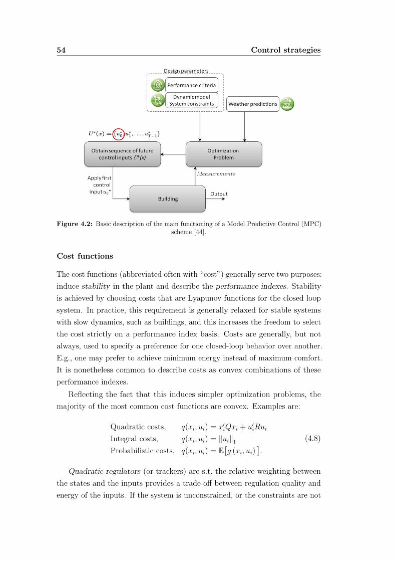
54 Control strategies
Figure 4.2: Basic description of the main functioning of a Model Predictive Control (MPC)scheme [44].
Cost functions
The cost functions (abbreviated often with “cost”) generally serve two purposes:
induce stability in the plant and describe the performance indexes. Stability
is achieved by choosing costs that are Lyapunov functions for the closed loop
system. In practice, this requirement is generally relaxed for stable systems
with slow dynamics, such as buildings, and this increases the freedom to select
the cost strictly on a performance index basis. Costs are generally, but not
always, used to specify a preference for one closed-loop behavior over another.
E.g., one may prefer to achieve minimum energy instead of maximum comfort.
It is nonetheless common to describe costs as convex combinations of these
performance indexes.
Reflecting the fact that this induces simpler optimization problems, the
majority of the most common cost functions are convex. Examples are:
Quadratic costs, q(xi, ui) = x′iQxi + u′iRui
Integral costs, q(xi, ui) = ‖ui‖1
Probabilistic costs, q(xi, ui) = E[g (xi, ui)
].
(4.8)
Quadratic regulators (or trackers) are s.t. the relative weighting between
the states and the inputs provides a trade-off between regulation quality and
energy of the inputs. If the system is unconstrained, or the constraints are not
4.2 The considered Model Predictive Control (MPC) strategy 55
active, then the problem reduces to a classic Linear Quadratic Regulator (LQR).
In the context of building control scenarios, such a cost would generally only
be used at the lowest level to replace, for example, existing PIs or rule-based
controllers.
Integral costs, instead, weight the integral of the energy of the inputs. This
is a common choice whenever the performance index is the minimization of the
used energy.
Probabilistic costs are eventually tailored for system subject to random
disturbances. In this way users may choose to take into account the stochastic
nature of certain phenomena, and to minimize some expected value of some
event (or transformation of events), such as room comfort bounds violations.
Dynamics
The dynamics of the to-be-controlled system are represented by two distinct
parts: the initial conditions and the time evolution.
General MPC strategies require to initialize the model of the system at
each time step. This is performed usually by forcing the state of this system
to be equal to the measured / estimated current state. In this way all the
future control predictions begin from a system that is initialized every time in
a different way. We also notice that this strategy is not the unique one: certain
robust MPC strategies for example assume the current state to be not known
exactly, but only to belong to a bounded set.
Assuming the initial conditions to be set, to predict the future states
numerical optimizers need a model of the evolution of the system. Modeling
the dynamics of the system plays a critical role in MPC frameworks: indeed,
if the model of the temporal evolution of the plant is grossly mistaken then
the numerical optimizers will return control plans that may eventually lead to
very poor control performance. The most common models considered in MPC
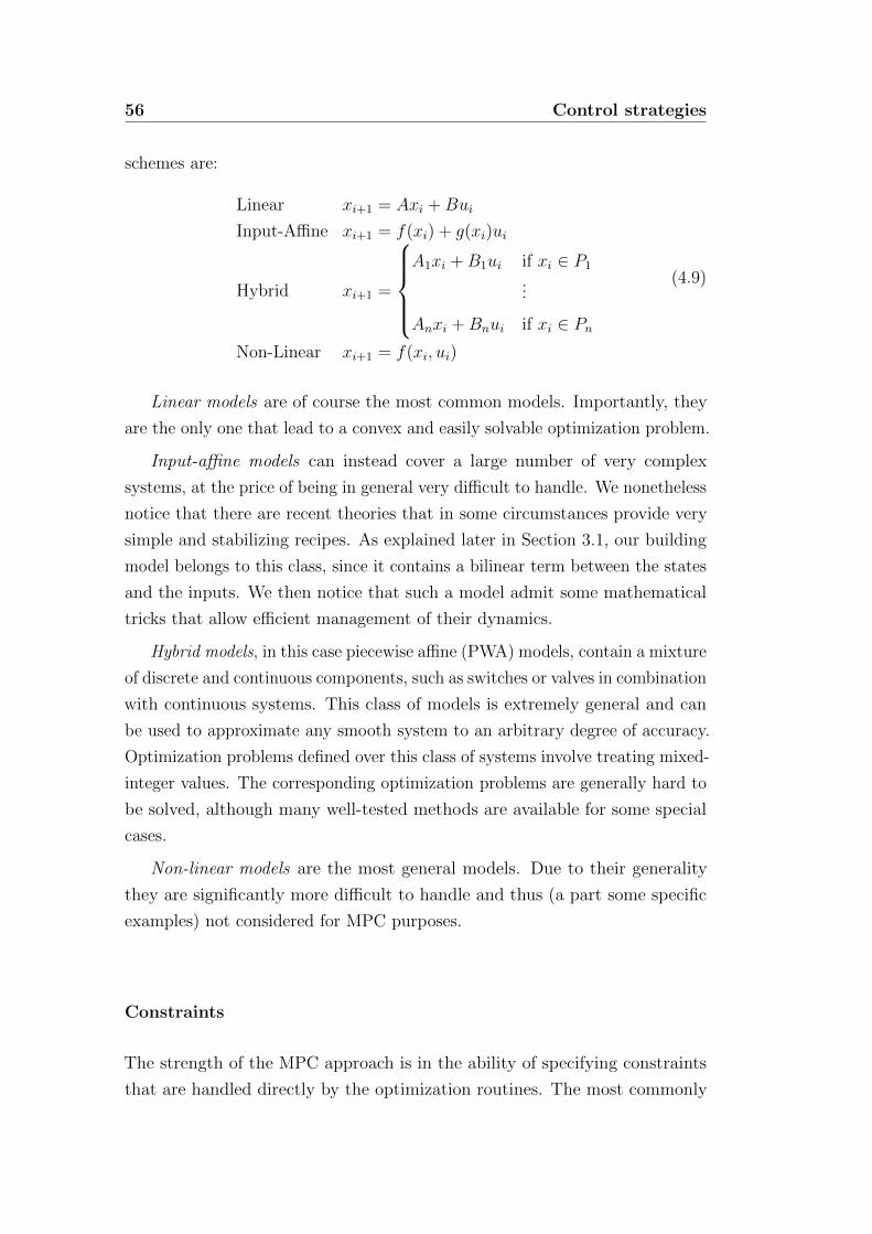
56 Control strategies
schemes are:
Linear xi+1 = Axi +Bui
Input-Affine xi+1 = f(xi) + g(xi)ui
Hybrid xi+1 =
A1xi +B1ui if xi ∈ P1
...
Anxi +Bnui if xi ∈ PnNon-Linear xi+1 = f(xi, ui)
(4.9)
Linear models are of course the most common models. Importantly, they
are the only one that lead to a convex and easily solvable optimization problem.
Input-affine models can instead cover a large number of very complex
systems, at the price of being in general very difficult to handle. We nonetheless
notice that there are recent theories that in some circumstances provide very
simple and stabilizing recipes. As explained later in Section 3.1, our building
model belongs to this class, since it contains a bilinear term between the states
and the inputs. We then notice that such a model admit some mathematical
tricks that allow efficient management of their dynamics.
Hybrid models, in this case piecewise affine (PWA) models, contain a mixture
of discrete and continuous components, such as switches or valves in combination
with continuous systems. This class of models is extremely general and can
be used to approximate any smooth system to an arbitrary degree of accuracy.
Optimization problems defined over this class of systems involve treating mixed-
integer values. The corresponding optimization problems are generally hard to
be solved, although many well-tested methods are available for some special
cases.
Non-linear models are the most general models. Due to their generality
they are significantly more difficult to handle and thus (a part some specific
examples) not considered for MPC purposes.
Constraints
The strength of the MPC approach is in the ability of specifying constraints
that are handled directly by the optimization routines. The most commonly
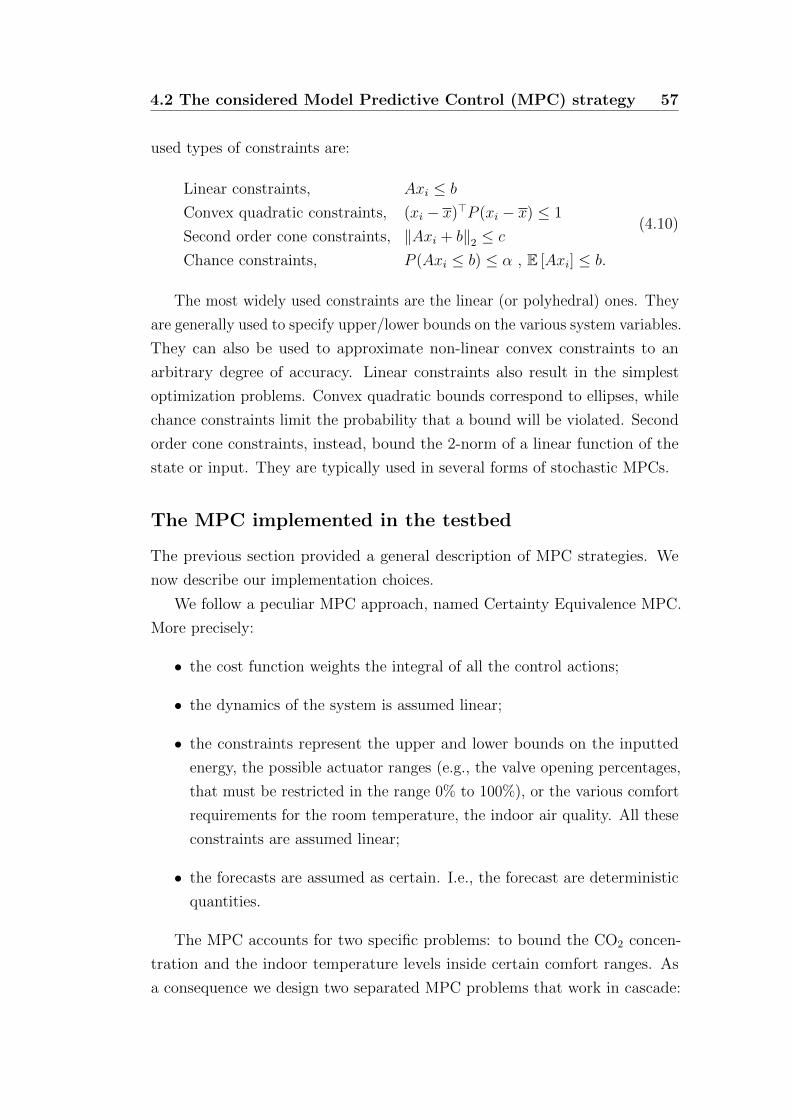
4.2 The considered Model Predictive Control (MPC) strategy 57
used types of constraints are:
Linear constraints, Axi ≤ b
Convex quadratic constraints, (xi − x)>P (xi − x) ≤ 1
Second order cone constraints, ‖Axi + b‖2 ≤ c
Chance constraints, P (Axi ≤ b) ≤ α , E [Axi] ≤ b.
(4.10)
The most widely used constraints are the linear (or polyhedral) ones. They
are generally used to specify upper/lower bounds on the various system variables.
They can also be used to approximate non-linear convex constraints to an
arbitrary degree of accuracy. Linear constraints also result in the simplest
optimization problems. Convex quadratic bounds correspond to ellipses, while
chance constraints limit the probability that a bound will be violated. Second
order cone constraints, instead, bound the 2-norm of a linear function of the
state or input. They are typically used in several forms of stochastic MPCs.
The MPC implemented in the testbed
The previous section provided a general description of MPC strategies. We
now describe our implementation choices.
We follow a peculiar MPC approach, named Certainty Equivalence MPC.
More precisely:
• the cost function weights the integral of all the control actions;
• the dynamics of the system is assumed linear;
• the constraints represent the upper and lower bounds on the inputted
energy, the possible actuator ranges (e.g., the valve opening percentages,
that must be restricted in the range 0% to 100%), or the various comfort
requirements for the room temperature, the indoor air quality. All these
constraints are assumed linear;
• the forecasts are assumed as certain. I.e., the forecast are deterministic
quantities.
The MPC accounts for two specific problems: to bound the CO2 concen-
tration and the indoor temperature levels inside certain comfort ranges. As
a consequence we design two separated MPC problems that work in cascade:
58 Control strategies
the first is dedicated to the management of the CO2 levels. The second to the
temperature. The first targets to return the minimal level of fresh air flow
that must enter in the room to maintain a certain comfort range. The second
instead computes the actuation commands to let the temperature be in its
comfort range.
The main performance index considered while designing the cost functions
is the amount of energy spent to maintain the internal comfort levels. The
optimization routines thus aim to find the control references that satisfy the air
quality levels while spending the least amount of energy. We also notice that we
consider two separated MPCs to obtain linear models, exploiting the fact that
the dynamics of the CO2 levels is decoupled from the one of the temperature.
The designed MPC cycles the following steps:
1. build a model of the physical variables of interest (if it changes at each
sample time);
2. take the local measurements;
3. build weather / occupancy / solar radiation predictions;
4. build the MPC formulation and construct the constraints;
5. solve the linear problem deriving from the previous step;
6. apply the computed control actions (only the first sample, in accordance
with the MPC paradigm);
7. wait the next sample time and repeat the procedure.
The models (3.3) and (3.15) described in Section 3.1 contain nonlinearities
that can lead to intractable problems. To address this issue we derive linear
equivalent formulations of the CO2 concentration model (in Section 3.1) and of
the room thermal model (in Section 3.1).
The CO2 MPC
To linearize the CO2 concentration dynamics, as already considered in (3.15)
and also in the identification that carried to that expression, we replace the
nonlinear term mair·(CCO2−CCO2,i) with uCO2 , where CCO2,i is the concentration
of the air that is flowing inside. We can consider it like a constant (with the
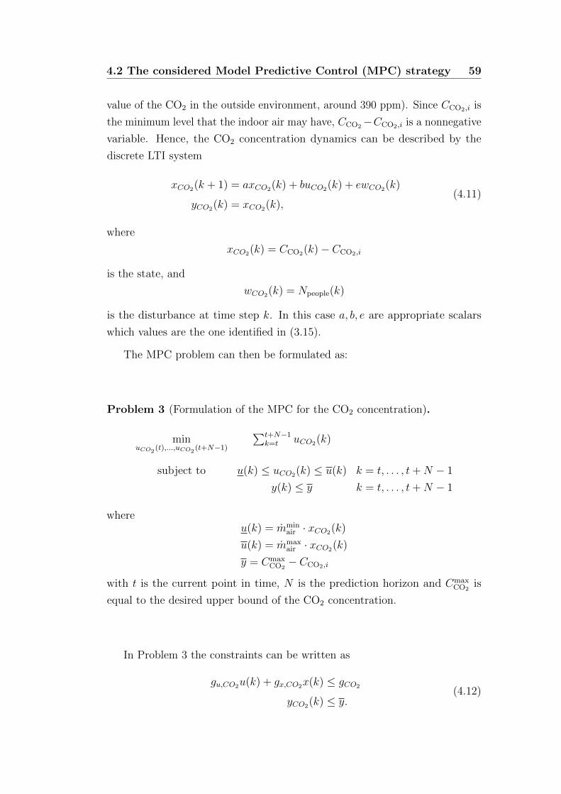
4.2 The considered Model Predictive Control (MPC) strategy 59
value of the CO2 in the outside environment, around 390 ppm). Since CCO2,i is
the minimum level that the indoor air may have, CCO2−CCO2,i is a nonnegative
variable. Hence, the CO2 concentration dynamics can be described by the
discrete LTI system
xCO2(k + 1) = axCO2(k) + buCO2(k) + ewCO2(k)
yCO2(k) = xCO2(k),(4.11)
where
xCO2(k) = CCO2(k)− CCO2,i
is the state, and
wCO2(k) = Npeople(k)
is the disturbance at time step k. In this case a, b, e are appropriate scalars
which values are the one identified in (3.15).
The MPC problem can then be formulated as:
Problem 3 (Formulation of the MPC for the CO2 concentration).
minuCO2
(t),...,uCO2(t+N−1)
∑t+N−1k=t uCO2(k)
subject to u(k) ≤ uCO2(k) ≤ u(k) k = t, . . . , t+N − 1
y(k) ≤ y k = t, . . . , t+N − 1
whereu(k) = mmin
air · xCO2(k)
u(k) = mmaxair · xCO2(k)
y = CmaxCO2− CCO2,i
with t is the current point in time, N is the prediction horizon and CmaxCO2
is
equal to the desired upper bound of the CO2 concentration.
In Problem 3 the constraints can be written as
gu,CO2u(k) + gx,CO2x(k) ≤ gCO2
yCO2(k) ≤ y.(4.12)
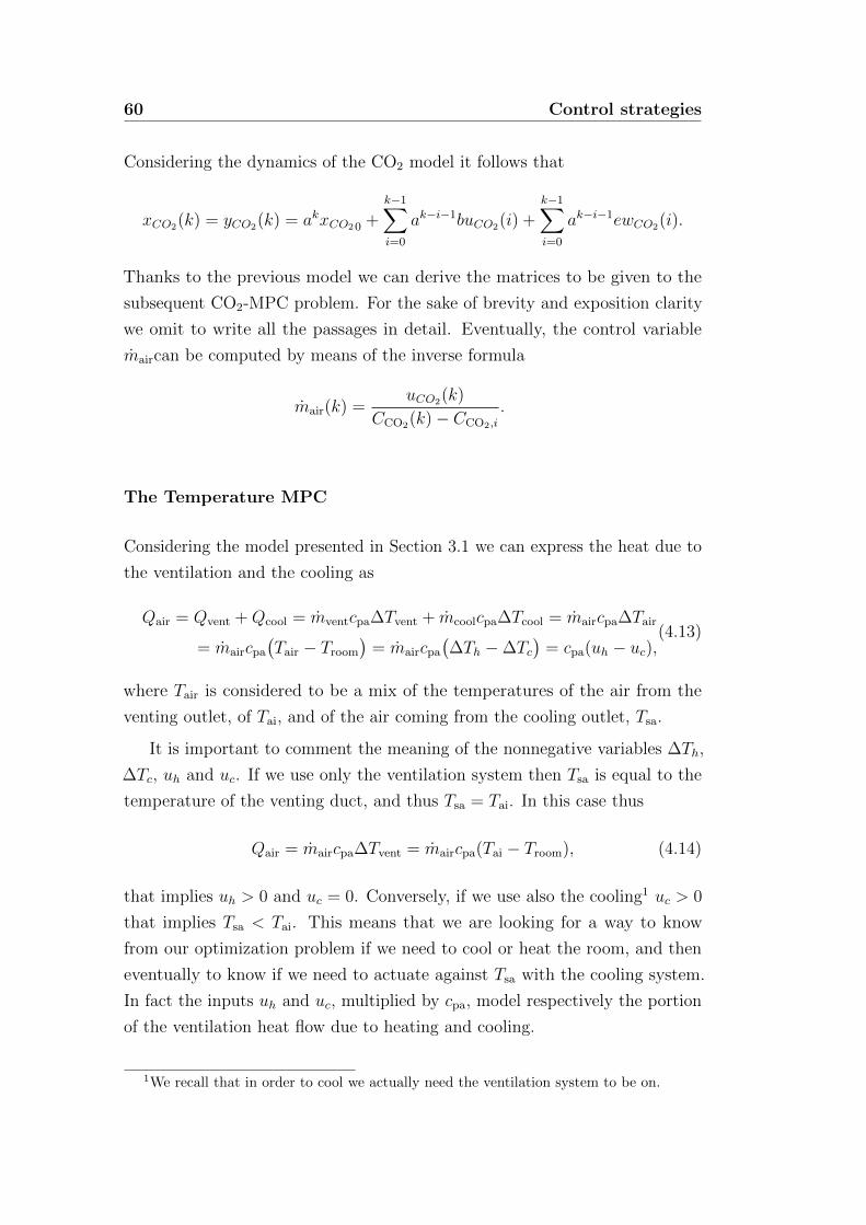
60 Control strategies
Considering the dynamics of the CO2 model it follows that
xCO2(k) = yCO2(k) = akxCO20 +k−1∑i=0
ak−i−1buCO2(i) +k−1∑i=0
ak−i−1ewCO2(i).
Thanks to the previous model we can derive the matrices to be given to the
subsequent CO2-MPC problem. For the sake of brevity and exposition clarity
we omit to write all the passages in detail. Eventually, the control variable
maircan be computed by means of the inverse formula
mair(k) =uCO2(k)
CCO2(k)− CCO2,i
.
The Temperature MPC
Considering the model presented in Section 3.1 we can express the heat due to
the ventilation and the cooling as
Qair = Qvent +Qcool = mventcpa∆Tvent + mcoolcpa∆Tcool = maircpa∆Tair
= maircpa
(Tair − Troom
)= maircpa
(∆Th −∆Tc
)= cpa(uh − uc),
(4.13)
where Tair is considered to be a mix of the temperatures of the air from the
venting outlet, of Tai, and of the air coming from the cooling outlet, Tsa.
It is important to comment the meaning of the nonnegative variables ∆Th,
∆Tc, uh and uc. If we use only the ventilation system then Tsa is equal to the
temperature of the venting duct, and thus Tsa = Tai. In this case thus
Qair = maircpa∆Tvent = maircpa(Tai − Troom), (4.14)
that implies uh > 0 and uc = 0. Conversely, if we use also the cooling1 uc > 0
that implies Tsa < Tai. This means that we are looking for a way to know
from our optimization problem if we need to cool or heat the room, and then
eventually to know if we need to actuate against Tsa with the cooling system.
In fact the inputs uh and uc, multiplied by cpa, model respectively the portion
of the ventilation heat flow due to heating and cooling.
1We recall that in order to cool we actually need the ventilation system to be on.
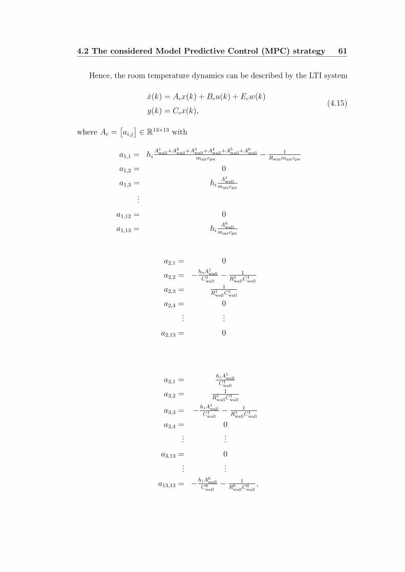
4.2 The considered Model Predictive Control (MPC) strategy 61
Hence, the room temperature dynamics can be described by the LTI system
x(k) = Acx(k) +Bcu(k) + Ecw(k)
y(k) = Ccx(k),(4.15)
where Ac =[ai,j]∈ R13×13 with
a1,1 = hiA1
wall+A2wall+A
3wall+A
4wall+A
5wall+A
6wall
maircpa− 1
Rwinmaircpa
a1,2 = 0
a1,3 = hiA1
wall
maircpa
...
a1,12 = 0
a1,13 = hiA6
wall
maircpa
a2,1 = 0
a2,2 = −hoA1wall
C1wall− 1
R1wallC
1wall
a2,3 = 1R1
wallC1wall
a2,4 = 0...
...
a2,13 = 0
a3,1 =hiA
1wall
C1wall
a3,2 = 1R1
wallC1wall
a3,3 = −hiA1wall
C1wall− 1
R1wallC
1wall
a3,4 = 0...
...
a3,13 = 0...
...
a13,13 = −hiA6wall
C6wall− 1
R6wallC
6wall,
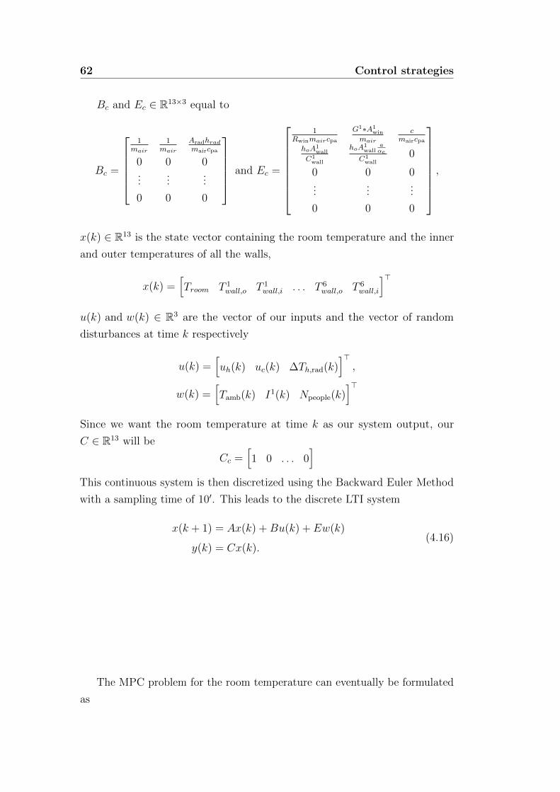
62 Control strategies
Bc and Ec ∈ R13×3 equal to
Bc =
1
mair
1mair
Aradhradmaircpa
0 0 0...
......
0 0 0
and Ec =
1Rwinmaircpa
G1∗A1win
mair
cmaircpa
hoA1wall
C1wall
hoA1wall
aαe
C1wall
0
0 0 0...
......
0 0 0
,
x(k) ∈ R13 is the state vector containing the room temperature and the inner
and outer temperatures of all the walls,
x(k) =[Troom T 1
wall,o T 1wall,i . . . T 6
wall,o T 6wall,i
]>u(k) and w(k) ∈ R3 are the vector of our inputs and the vector of random
disturbances at time k respectively
u(k) =[uh(k) uc(k) ∆Th,rad(k)
]>,
w(k) =[Tamb(k) I1(k) Npeople(k)
]>Since we want the room temperature at time k as our system output, our
C ∈ R13 will be
Cc =[1 0 . . . 0
]This continuous system is then discretized using the Backward Euler Method
with a sampling time of 10′. This leads to the discrete LTI system
x(k + 1) = Ax(k) +Bu(k) + Ew(k)
y(k) = Cx(k).(4.16)
The MPC problem for the room temperature can eventually be formulated
as
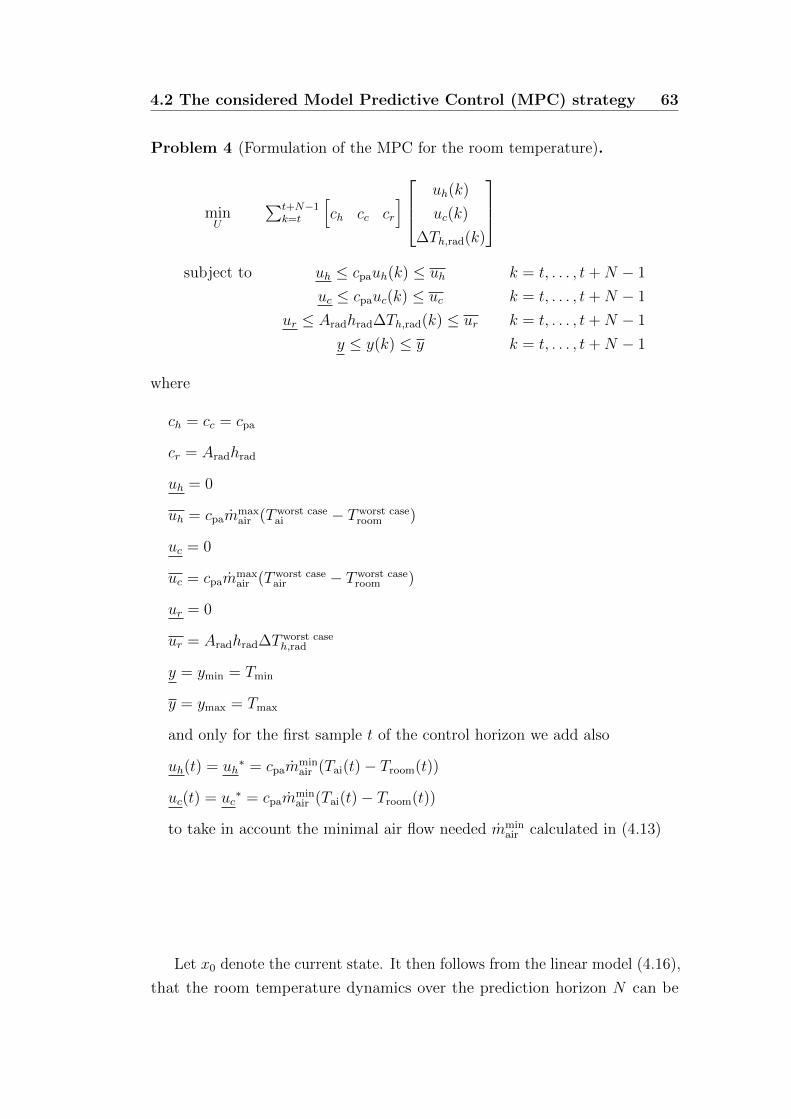
4.2 The considered Model Predictive Control (MPC) strategy 63
Problem 4 (Formulation of the MPC for the room temperature).
minU
∑t+N−1k=t
[ch cc cr
] uh(k)
uc(k)
∆Th,rad(k)
subject to uh ≤ cpauh(k) ≤ uh k = t, . . . , t+N − 1
uc ≤ cpauc(k) ≤ uc k = t, . . . , t+N − 1
ur ≤ Aradhrad∆Th,rad(k) ≤ ur k = t, . . . , t+N − 1
y ≤ y(k) ≤ y k = t, . . . , t+N − 1
where
ch = cc = cpa
cr = Aradhrad
uh = 0
uh = cpammaxair (Tworst case
ai − Tworst caseroom )
uc = 0
uc = cpammaxair (Tworst case
air − Tworst caseroom )
ur = 0
ur = Aradhrad∆Tworst caseh,rad
y = ymin = Tmin
y = ymax = Tmax
and only for the first sample t of the control horizon we add also
uh(t) = uh∗ = cpam
minair (Tai(t)− Troom(t))
uc(t) = uc∗ = cpam
minair (Tai(t)− Troom(t))
to take in account the minimal air flow needed mminair calculated in (4.13)
Let x0 denote the current state. It then follows from the linear model (4.16),
that the room temperature dynamics over the prediction horizon N can be
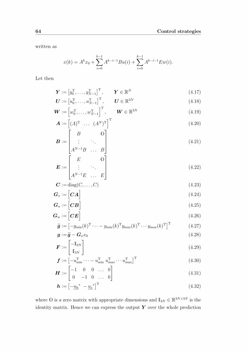
64 Control strategies
written as
x(k) = Akx0 +k−1∑i=0
Ak−i−1Bu(i) +k−1∑i=0
Ak−i−1Ew(i).
Let then
Y :=[yT
0 , . . . , yTN−1
]T, Y ∈ RN (4.17)
U :=[uT
0 , . . . , uTN−1
]T, U ∈ R3N (4.18)
W :=[wT
0 , . . . , wTN−1
]T
, W ∈ R3N (4.19)
A :=[(A)T . . . (AN)T
]T
(4.20)
B :=
B O...
. . .
AN−1B . . . B
(4.21)
E :=
E O...
. . .
AN−1E . . . E
(4.22)
C := diag(C, . . . , C) (4.23)
Gx :=[CA
](4.24)
Gu :=[CB
](4.25)
Gw :=[CE
](4.26)
g :=[−ymin(k)T · · · − ymin(k)Tymax(k)T · · · ymax(k)T
]T(4.27)
g := g −Gxx0 (4.28)
F :=
[−I3N
I3N
](4.29)
f :=[−uT
min · · · − uTmin u
Tmax · · ·uT
max
]T(4.30)
H :=
[−1 0 0 . . . 0
0 −1 0 . . . 0
](4.31)
h :=[−uh∗ − uc∗
]T(4.32)
where O is a zero matrix with appropriate dimensions and I3N ∈ R3N×3N is the
identity matrix. Hence we can express the output Y over the whole prediction
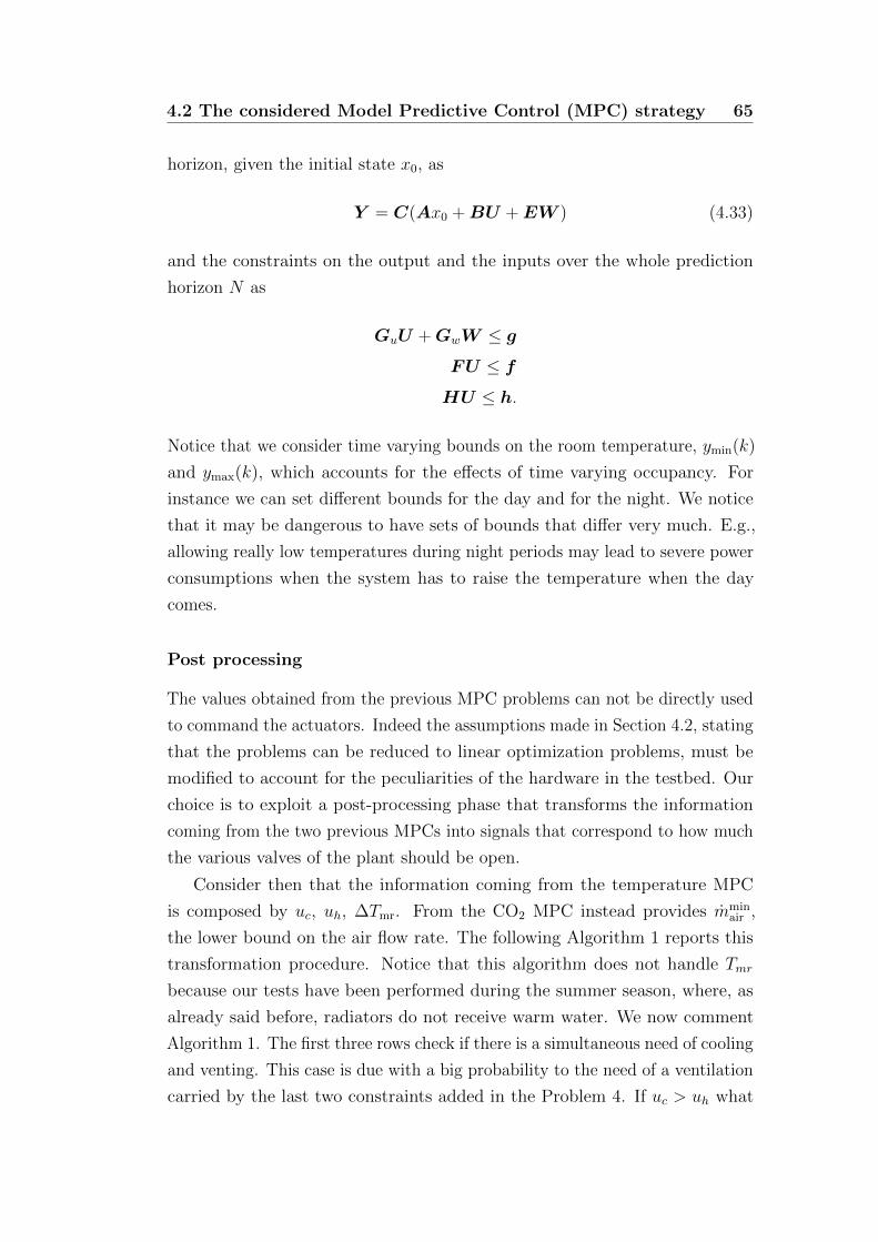
4.2 The considered Model Predictive Control (MPC) strategy 65
horizon, given the initial state x0, as
Y = C(Ax0 + BU + EW ) (4.33)
and the constraints on the output and the inputs over the whole prediction
horizon N as
GuU + GwW ≤ g
FU ≤ f
HU ≤ h.
Notice that we consider time varying bounds on the room temperature, ymin(k)
and ymax(k), which accounts for the effects of time varying occupancy. For
instance we can set different bounds for the day and for the night. We notice
that it may be dangerous to have sets of bounds that differ very much. E.g.,
allowing really low temperatures during night periods may lead to severe power
consumptions when the system has to raise the temperature when the day
comes.
Post processing
The values obtained from the previous MPC problems can not be directly used
to command the actuators. Indeed the assumptions made in Section 4.2, stating
that the problems can be reduced to linear optimization problems, must be
modified to account for the peculiarities of the hardware in the testbed. Our
choice is to exploit a post-processing phase that transforms the information
coming from the two previous MPCs into signals that correspond to how much
the various valves of the plant should be open.
Consider then that the information coming from the temperature MPC
is composed by uc, uh, ∆Tmr. From the CO2 MPC instead provides mminair ,
the lower bound on the air flow rate. The following Algorithm 1 reports this
transformation procedure. Notice that this algorithm does not handle Tmr
because our tests have been performed during the summer season, where, as
already said before, radiators do not receive warm water. We now comment
Algorithm 1. The first three rows check if there is a simultaneous need of cooling
and venting. This case is due with a big probability to the need of a ventilation
carried by the last two constraints added in the Problem 4. If uc > uh what
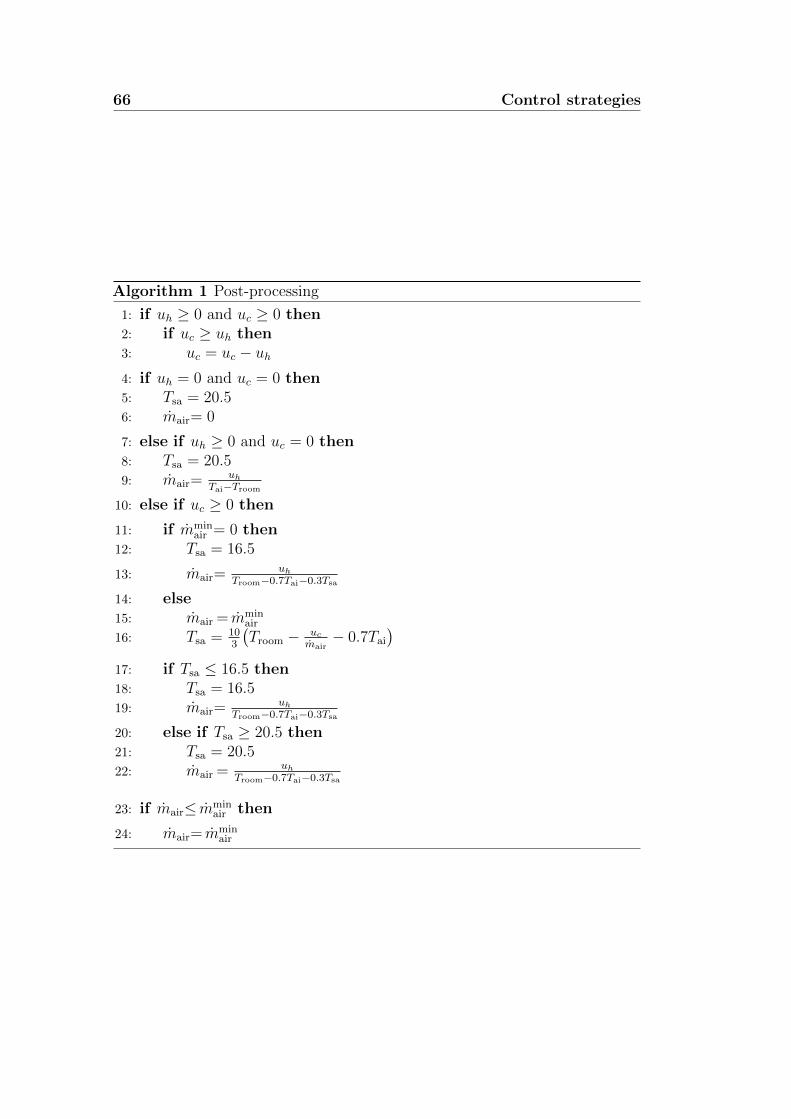
66 Control strategies
Algorithm 1 Post-processing
1: if uh ≥ 0 and uc ≥ 0 then2: if uc ≥ uh then3: uc = uc − uh4: if uh = 0 and uc = 0 then5: Tsa = 20.56: mair= 0
7: else if uh ≥ 0 and uc = 0 then8: Tsa = 20.59: mair=
uhTai−Troom
10: else if uc ≥ 0 then
11: if mminair = 0 then
12: Tsa = 16.5
13: mair=uh
Troom−0.7Tai−0.3Tsa
14: else15: mair = mmin
air
16: Tsa = 103
(Troom − uc
mair− 0.7Tai
)17: if Tsa ≤ 16.5 then18: Tsa = 16.519: mair=
uhTroom−0.7Tai−0.3Tsa
20: else if Tsa ≥ 20.5 then21: Tsa = 20.522: mair = uh
Troom−0.7Tai−0.3Tsa
23: if mair≤ mminair then
24: mair= mminair
4.2 The considered Model Predictive Control (MPC) strategy 67
actually we have to do is to cool uc − uh. The opposite situation is managed
from the row 10. From row 4 to 6 we are setting instead the parameters in
order not to actuate anything. In fact the temperature of the cooling supply
air is in average between 16.5 the lowest temperature we saw from several
measurements, and 20.5, the average temperature of the air inlet flow. From
the row 7 to 9 we are facing the need of ventilation. That could be for heating
purposes, fresh air purposes or also, accordingly with the temperature of the
room, also for cooling purposes. If there is no need of cooling, it means that all
the uv will be translated to mair from the reverse formulation of (4.14). From
the row 10 we are checking the need of cooling. The first step is to check the
lower bound of the CO2 model. If it is 0 we cool at the lowest temperature,
trying to minimize the air mass flow2. The formula in the row 13 come from
the knowledge exposed in the Subsection 3.2 of a kind of average ratio of 3÷ 7
between the cooling air flow (mcool) and the venting air flow3 (mvent). We can
in fact think at the uc as
uc = mair
(Troom − Tair
)= mair
(Troom − 0.7Tai − 0.3Tsa
), (4.34)
considering Tair like a mixture of air form the two different branches. From the
equation (4.34) are coming also the formulas in the rows 19 and 22, used to
bound eventually cases where the formula in the row 13 takes us to lower or
higher values of Tsa, that are set in the limits of our comfort range.
At the end we do a security check to be sure that the value that actually we
are giving it is greater than the required lower bound. If at the end we have an
mair different from 0[kg/s] it means that we have to actuate the corresponding
percentage for the venting valve. Viceversa, if we have a Tsa that is lower than
20 it means that we have to cool the room.
Transformation of the commands given by the CO2 and
temperature MPC into valves openings signals
The outcomes given by the previously described MPCs must be transformed
into values for
1. ∆Th,rad, i.e., how much the valve relative to the radiators should be open;
2This is due to follow our assumption of a lower cost for the cooling action compared tothe venting action
3The part that is coming only from the venting branch
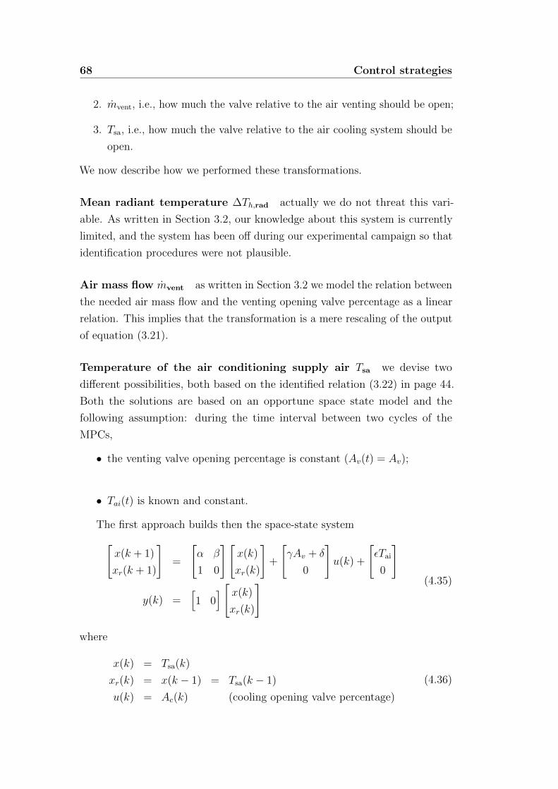
68 Control strategies
2. mvent, i.e., how much the valve relative to the air venting should be open;
3. Tsa, i.e., how much the valve relative to the air cooling system should be
open.
We now describe how we performed these transformations.
Mean radiant temperature ∆Th,rad actually we do not threat this vari-
able. As written in Section 3.2, our knowledge about this system is currently
limited, and the system has been off during our experimental campaign so that
identification procedures were not plausible.
Air mass flow mvent as written in Section 3.2 we model the relation between
the needed air mass flow and the venting opening valve percentage as a linear
relation. This implies that the transformation is a mere rescaling of the output
of equation (3.21).
Temperature of the air conditioning supply air Tsa we devise two
different possibilities, both based on the identified relation (3.22) in page 44.
Both the solutions are based on an opportune space state model and the
following assumption: during the time interval between two cycles of the
MPCs,
• the venting valve opening percentage is constant (Av(t) = Av);
• Tai(t) is known and constant.
The first approach builds then the space-state system[x(k + 1)
xr(k + 1)
]=
[α β
1 0
][x(k)
xr(k)
]+
[γAv + δ
0
]u(k) +
[εTai
0
]
y(k) =[1 0
] [ x(k)
xr(k)
] (4.35)
where
x(k) = Tsa(k)
xr(k) = x(k − 1) = Tsa(k − 1)
u(k) = Ac(k) (cooling opening valve percentage)
(4.36)
4.2 The considered Model Predictive Control (MPC) strategy 69
At this point system (4.35) can be written as x(k + 1)
xr(k + 1)
= A
[x(k)
xr(k)
]+Bu(k) + E
y(k) = C
[x(k)
xr(k)
] (4.37)
Considering the constant input Ureg that carries the system to the equilibrium
point x = Tsa,ref we find
x(k + 1) = x = Ax+BUreg + E. (4.38)
Solving the previous equation gives
Ureg =(B>B
)B>[(I − A
)x− E
](4.39)
It can be noticed that this kind of control law does not rely on feedback
mechanisms.
The second solution is instead developed as follows: start from (4.35), and
consider that we have a system with a constant disturbance on the state (the
constant matrix E). Let then the input be ∆u(k) rather than u(k). Adding
the state
xu(k) = u(k − 1) (4.40)
the whole system becomes x(k + 1)
xr(k + 1)
xu(k + 1)
=
α β γAv + δ
1 0 0
0 0 1
x(k)
xr(k)
xe(k)
+
γAv + δ
0
1
∆u(k) +
εTai
0
0
y(k) =[1 0 0
] x(k)
xr(k)
xe(k)
(4.41)
70 Control strategies
that can also written as x(k + 1)
xr(k + 1)
xu(k + 1)
= A
x(k)
xr(k)
xu(k)
+B∆u(k) + E
y(k) = C
x(k)
xr(k)
xu(k)
.(4.42)
The optimal input can then be found as the solution of the following optimization
problem:
Problem 5 (Formulation of the MPC for the control of the cooling actuation).
min∆u(t),...,∆u(t+N−1)
∑t+N−1k=t
∥∥∥W y[y(k + 1)− r∗
]∥∥∥2
+∥∥∥W∆u∆u(k)
∥∥∥2
subject to u ≤ u(k) ≤ u k = t, . . . , t+N − 1
∆u ≤ ∆u(k) ≤ ∆u k = t, . . . , t+N − 1
y ≤ y(k) ≤ y k = t, . . . , t+N − 1
(4.43)
The constraint on u(t), ∆u(t), y(t) can be expressed as:
HA xt + HB ∆U + HE 1N×1 ≤ u 1N×1
HA xt + HB ∆U + HE 1N×1 ≥ u 1N×1
I∆U ≤ ∆u1N×1
I∆U ≥ ∆u1N×1
CA xt + CB ∆U + CE 1N×1 ≤ y 1N×1
CA xt + CB ∆U + CE 1N×1 ≥ y 1N×1
(4.44)
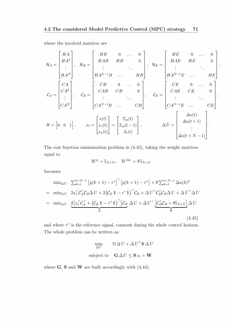
4.2 The considered Model Predictive Control (MPC) strategy 71
where the involved matrices are
HA =
HA
HA2
...
HAN
, HB =
HB 0 . . . 0
HAB HB 0...
. . .
HAN−1B . . . HB
, HE =
HE 0 . . . 0
HAE HE 0...
. . .
HAN−1E . . . HE
,
CA =
CA
CA2
...
CAN
, CB =
CB 0 . . . 0
CAB CB 0...
. . .
CAN−1B . . . CB
, CE =
CE 0 . . . 0
CAE CE 0...
. . .
CAN−1E . . . CE
,
H =[0 0 1
], xt =
x(t)
xr(t)
xu(t)
=
Tsa(t)
Tsa(t− 1)
Ac(t)
, ∆U =
∆u(t)
∆u(t + 1)...
∆u(t + N − 1)
.
The cost function minimization problem in (4.43), taking the weight matrices
equal to
W y = IN×N , W∆u = θ IN×N
becomes
min∆U
∑t+N−1k=t
[y(k + 1)− r∗
]>[y(k + 1)− r∗
]+ θ
∑t+N−1k=t ∆u(k)2
= min∆U 2x>t C>ACB∆U + 2(CE 1− r∗ 1
)>CB + ∆U>C>BCB∆U + ∆U>∆U
= min∆U 2[x>t C>A +
(CE 1− r∗ 1
)>]CB︸ ︷︷ ︸Ω
∆U + ∆U>[C>BCB + θIN×N
]︸ ︷︷ ︸Φ
∆U
(4.45)
and where r∗ is the reference signal, constant during the whole control horizon.
The whole problem can be written as:
min∆U
Ω ∆U + ∆U>Φ ∆U
subject to G ∆U ≤ Sxt + W
where G, S and W are built accordingly with (4.44).

72 Control strategies

5Experimental Results
5.1 Testing the MPC solution adopted to
control the cooling actuation
Before testing the whole MPC strategy we tested the second level controller
presented in Section 4.2 at page 67. This controller receives from the main
MPC a constant venting percentage and a reference Tsa and then aims to carry
the system to that reference in less than two MPC sampling periods (10 seconds
in our case). We notice that we do not explore the numerous different situations
that the system may face, and present only a subset of the meaningful cases.
The first numerical example simulates an active ventilation with set point
at 30% and two different temperature references: 17 and 18. In both the
cases the initial condition is set to 20. Results plotted in Figure 5.1 and 5.2
indicate the validity of the proposed controller, since it reaches the reference
signal in both cases in less than 8′ without any error.
Before testing the whole MPC scheme we then check how the first proposed
implementation works on real systems. The following Figures 5.3 and 5.4
show that with a reference signal of 17 the Tsa perfectly reaches the target
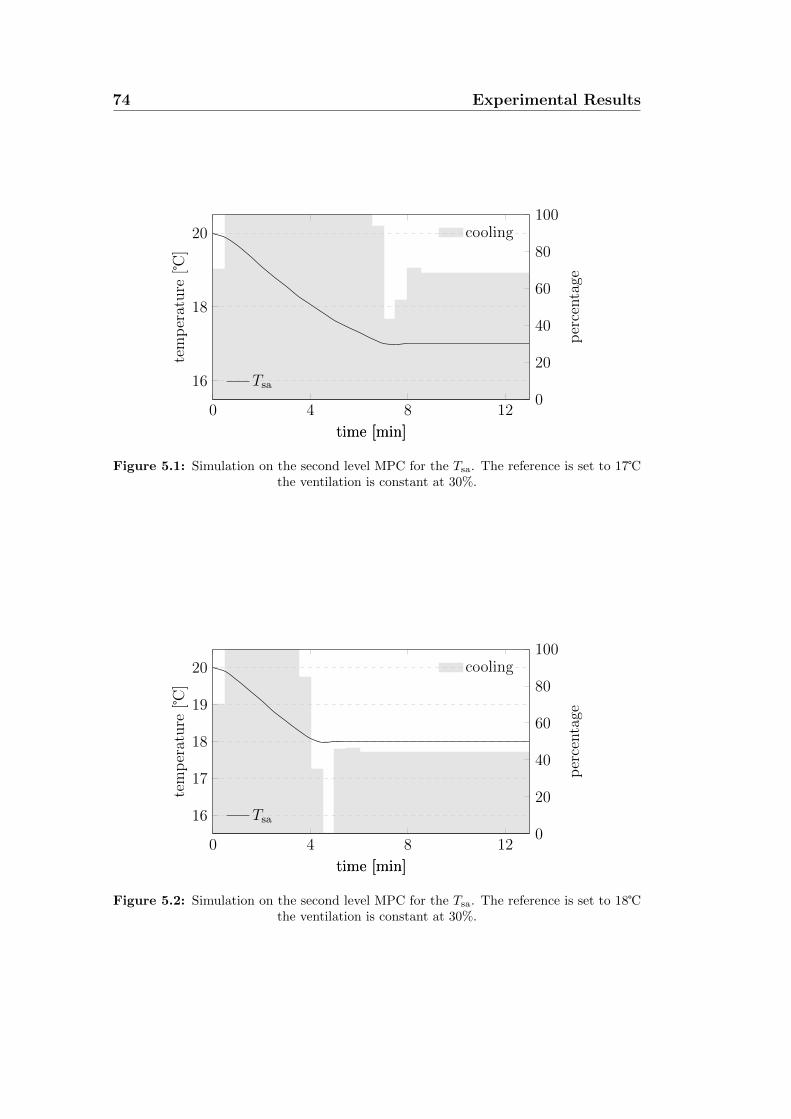
74 Experimental Results
0 4 8 120
20
40
60
80
100
time [min]
per
centa
ge
cooling
16
18
20
time [min]
tem
per
ature
[]
Tsa
Figure 5.1: Simulation on the second level MPC for the Tsa. The reference is set to 17the ventilation is constant at 30%.
0 4 8 120
20
40
60
80
100
time [min]
per
centa
ge
cooling
16
17
18
19
20
time [min]
tem
per
ature
[]
Tsa
Figure 5.2: Simulation on the second level MPC for the Tsa. The reference is set to 18the ventilation is constant at 30%.
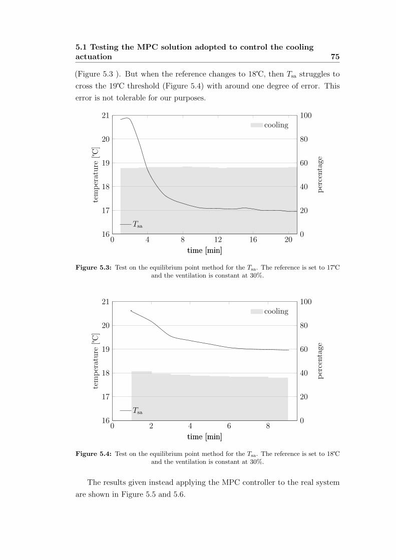
5.1 Testing the MPC solution adopted to control the coolingactuation 75
(Figure 5.3 ). But when the reference changes to 18, then Tsa struggles to
cross the 19 threshold (Figure 5.4) with around one degree of error. This
error is not tolerable for our purposes.
0 4 8 12 16 200
20
40
60
80
100
time [min]
per
centa
ge
cooling
16
17
18
19
20
21
time [min]
tem
per
ature
[]
Tsa
Figure 5.3: Test on the equilibrium point method for the Tsa. The reference is set to 17and the ventilation is constant at 30%.
0 2 4 6 80
20
40
60
80
100
time [min]
per
centa
gecooling
16
17
18
19
20
21
time [min]
tem
per
ature
[]
Tsa
Figure 5.4: Test on the equilibrium point method for the Tsa. The reference is set to 18and the ventilation is constant at 30%.
The results given instead applying the MPC controller to the real system
are shown in Figure 5.5 and 5.6.
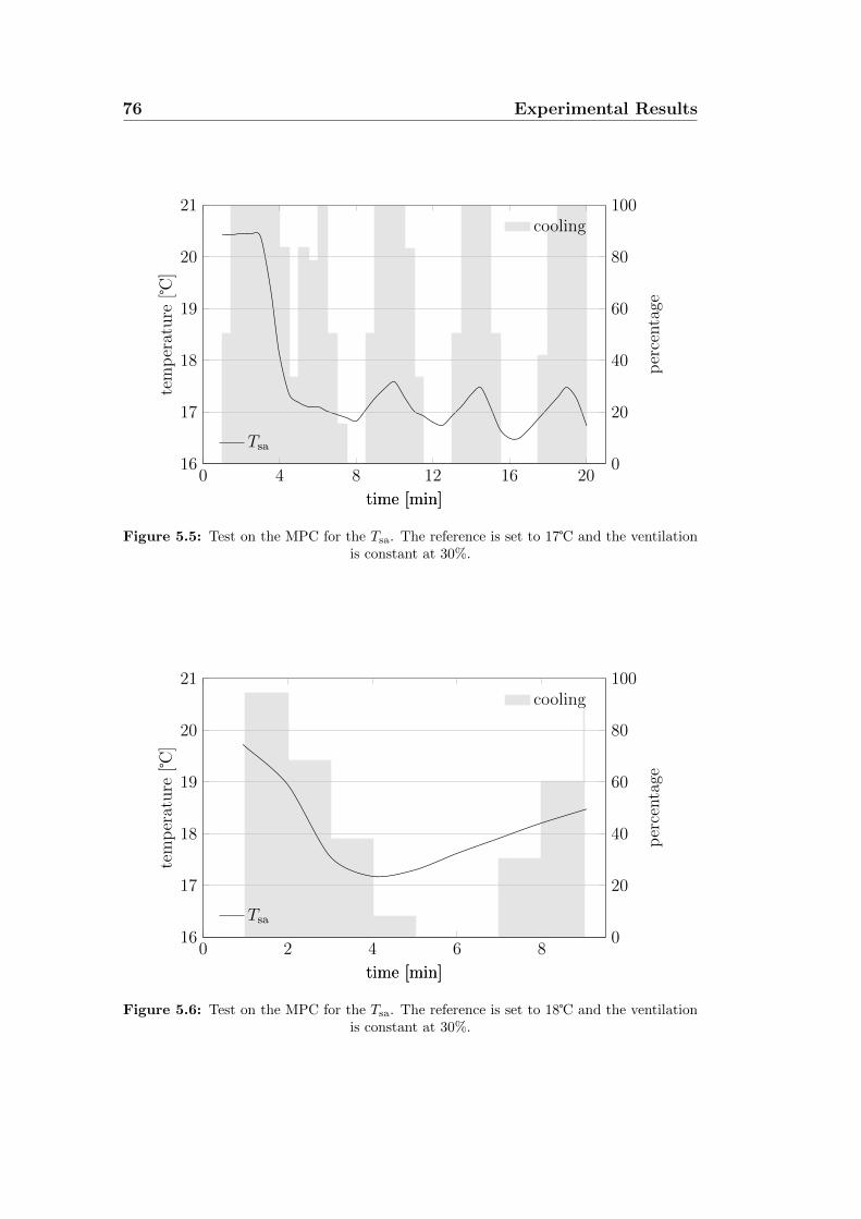
76 Experimental Results
0 4 8 12 16 200
20
40
60
80
100
time [min]
per
centa
ge
cooling
16
17
18
19
20
21
time [min]
tem
per
ature
[]
Tsa
Figure 5.5: Test on the MPC for the Tsa. The reference is set to 17 and the ventilationis constant at 30%.
0 2 4 6 80
20
40
60
80
100
time [min]
per
centa
ge
cooling
16
17
18
19
20
21
time [min]
tem
per
ature
[]
Tsa
Figure 5.6: Test on the MPC for the Tsa. The reference is set to 18 and the ventilationis constant at 30%.
5.2 Test of the whole MPC 77
We can notice that the equilibrium is never reached, and that there exists
a swinging response around the reference temperature. Furthermore the re-
quired temperature is never precisely reached. The comparison between these
controllers lead us to choose the second strategy to solve problem 5 because it
seems more reliable and respecting the conditions of the system.
5.2 Test of the whole MPC
We now present the results that we obtained applying our controller to the
testbed. To this aim we consider four separated tests.
We start describing how we selected the constraints more formally. As for
the bounds of the input commands, in all the tests we set them according to
some assumptions on the available power of our systems. We thus computed
these bounds starting from the equations for Qvent, Qcool and Qheat in (3.2) in
page 30 and from (3.14) at page 35 for uCO2 . We then choose to consider the
worst initial conditions that our system could face, and thus computed the
corresponding theoretically available power. For instance for the ventilation we
havemmin
air = 0 mminair ≈ 0.4
Tminai ≈ 20 Tmax
ai ≈ 22
Tminroom ≈ 15 Tmax
room ≈ 26.
With this assumption it follors
Qminair = 0
Qmaxair ≈ cpa
[J
KgK
]0.4[kgs
]· 7K ≈ 3kW < 3.5W.
The bound thus corresponds to
Qminvent = 0
Qmaxvent = 3.5kW
Qmincool = 0
Qmaxcool = 3kW
Qminrad = 0
Qmaxrad = 8kW
To test the CO2 MPC we used a slightly different approach, and set the
bounds accordingly with the status of the system. More precisely we assume
78 Experimental Results
that the CCO2,i concentration is constant, equal to the external one and thus
assumed to be 390 ppm. The bounds are thus set to
mminair
(xCO2(k)− CCO2,i
)≤ uCO2(k) ≤ mmax
air
(xCO2(k)− CCO2,i
)0 ≤ uCO2(k) ≤ 0.4
(xCO2(k)− 390
).
The bounds setting our comfort levels have then been derived using the
configuration suggested by Akademiska Hus. I.e., we copied the settings for
the controller described in Section 4.1 in page 49. The dead zone band band
adopted has thus been decided using a trade off between the wellness of the room
occupants. Notice that we did not force a small set of plausible temperatures
to our MPC solver: in this way we minimize risks of infeasible optimization
problems.
In total we set up 4 tests:
• Test 1:
– Temperature bounded between 20 to 23
– CO2 bounded under 700 ppm
– Period: 3 hours, between 11am and 2pm
The results are shown in Figure 5.7 at page 80
• Test 2:
– Temperature bounded between 20 to 23
– CO2 bounded under 700 ppm
– Period: 1.5 hours, between 2:30pm and 4pm
The results are shown in Figure 5.8 at page 81
• Test 3:
– Temperature bounded between 20 to 23
– CO2 bounded under 700 ppm
– Period: 3 hours, between 10am and 1pm
5.2 Test of the whole MPC 79
The results are shown in Figure 5.9 at page 82
• Test 4:
– Temperature bounded between 20 to 23
– CO2 bounded under 750 ppm
– Period: 1 hours, between 2pm and 3pm
The results are shown in Figure 5.9 at page 82
To run these tests we provide to our controller weather, thermal radiations and
occupancy forecasts. To this point we set:
• Weather forecasts: a linear interpolation of the hourly web forecasts
(described in Section 2.2 at page 24) accordingly with our sampling period
and our prediction horizon;
• Solar radiation forecasts: the tested area is not exposed to solar
radiation since it lies in the basements of the building. The windows are
either never hit by the solar rays or too small to let the solar radiation
influence significantly the comfort levels. Thereby we consider a null
effect for the whole period;
• Occupancy forecasts: to predict the occupancy we decided to use the
corresponding patterns of the very past week.
The proposed main MPC program runs every 10 minutes with a prediction
horizon of 8 hours. The low level MPC, as anticipated in Section 4.2 at page
67 and whose results are shown in Section 5.1, works when the main MPC
requires cooling actuation. From practical perspectives it works every minute
for the ten minutes needed. Figures 5.7, 5.8, 5.9, and 5.10 present the results
of our tests.
In all the tests the proposed control schemes respect almost everywhere the
comfort bounds. We indeed notice that during these experiments the room
temperature crossed the bound only few times and only for really short periods.
In all the cases the output of the CO2 MPC did not give to the temperature
MPC any bound. Test 4 then considers a case where the room occupancy is

80 Experimental Results
11:00 11:30 12:00 12:30 13:00 13:30 14:00
21.5
22
22.5
23
[]
Troom
460
480
500
520
[ppm
]
CO2
250500750
1,000
[W]
Qc
250500750
1,000
[W]
Qh
255075
100
[%]
venting cooling
16.5
18.5
20.5
22.5
[]
Tsa Tsa ref.
1234
[Np
eop
le] Npeople
11:00 11:30 12:00 12:30 13:00 13:30 14:00
18
19
20
[]
Tout
Figure 5.7: Test 1 on the MPC. The temperature comfort bounds are set to 20 to 23 while the upper bound of the CO2 concentration is 700 ppm.
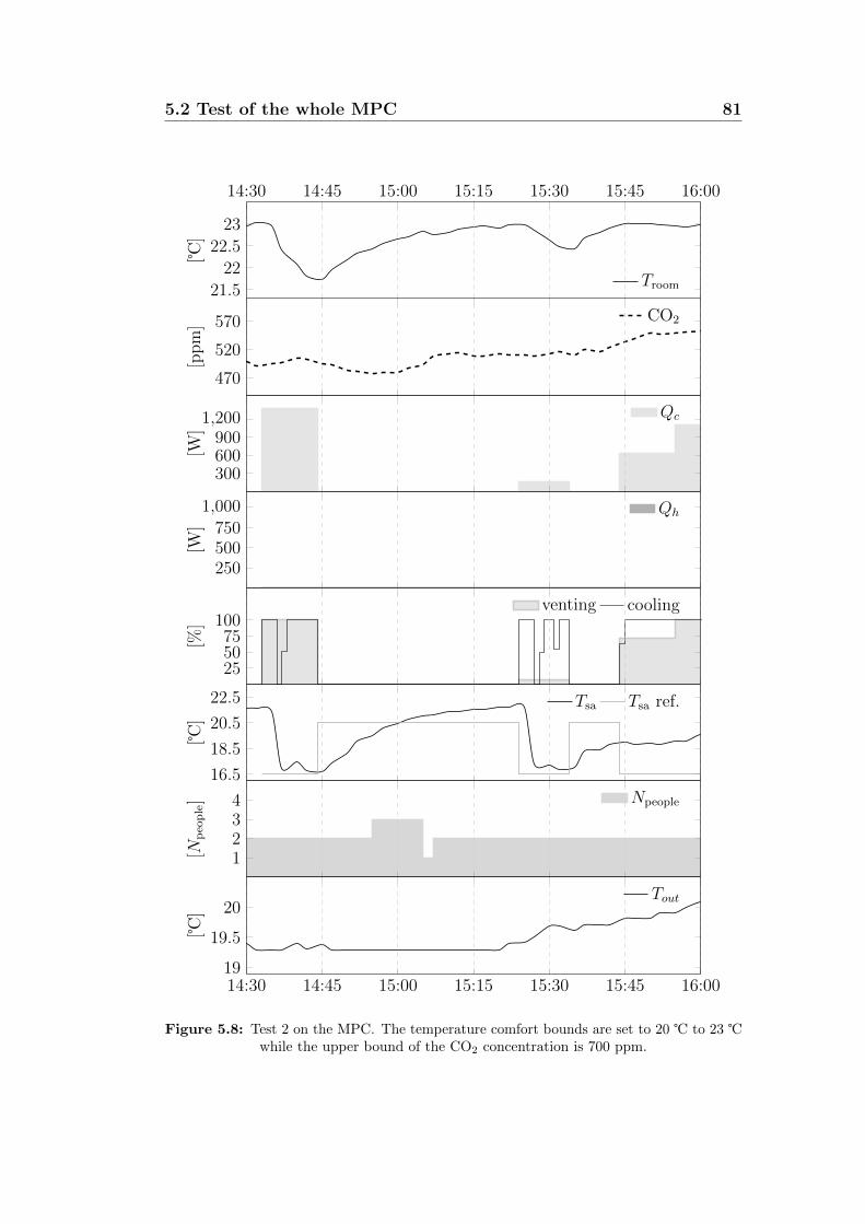
5.2 Test of the whole MPC 81
14:30 14:45 15:00 15:15 15:30 15:45 16:00
21.5
22
22.5
23
[]
Troom
470
520
570
[ppm
]
CO2
300600900
1,200
[W]
Qc
250500750
1,000
[W]
Qh
255075
100
[%]
venting cooling
16.5
18.5
20.5
22.5
[]
Tsa Tsa ref.
1234
[Np
eop
le] Npeople
14:30 14:45 15:00 15:15 15:30 15:45 16:0019
19.5
20
[]
Tout
Figure 5.8: Test 2 on the MPC. The temperature comfort bounds are set to 20 to 23 while the upper bound of the CO2 concentration is 700 ppm.
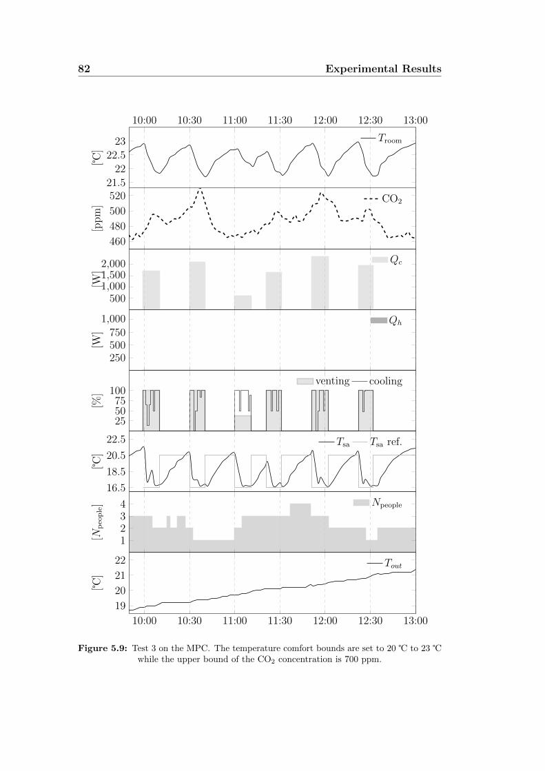
82 Experimental Results
10:00 10:30 11:00 11:30 12:00 12:30 13:00
21.5
22
22.5
23
[]
Troom
460
480
500
520
[ppm
]
CO2
5001,0001,5002,000
[W]
Qc
250500750
1,000
[W]
Qh
255075
100
[%]
venting cooling
16.5
18.5
20.5
22.5
[]
Tsa Tsa ref.
1234
[Np
eop
le] Npeople
10:00 10:30 11:00 11:30 12:00 12:30 13:00
19
20
21
22
[]
Tout
Figure 5.9: Test 3 on the MPC. The temperature comfort bounds are set to 20 to 23 while the upper bound of the CO2 concentration is 700 ppm.
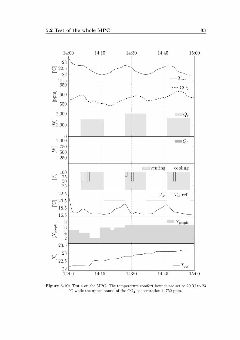
5.2 Test of the whole MPC 83
14:00 14:15 14:30 14:45 15:00
21.5
22
22.5
23
[]
Troom
550
600
650
[ppm
]
CO2
0
1,000
2,000
[W]
Qc
250500750
1,000
[W]
Qh
255075
100
[%]
venting cooling
16.5
18.5
20.5
22.5
[]
Tsa Tsa ref.
2468
[Np
eop
le] Npeople
14:00 14:15 14:30 14:45 15:0022
22.5
23
23.5
[]
Tout
Figure 5.10: Test 4 on the MPC. The temperature comfort bounds are set to 20 to 23 while the upper bound of the CO2 concentration is 750 ppm.
84 Experimental Results
very high, meaning thus a hight CO2 production rate. Even in this case no
lower bounds has been reached: first of all the CO2 concentration never reached
alert levels. This is also thanks to the Temperature MPC, that with its effort
to decrease the temperature provided an additional boost to the ventilation
system and thus helping the CO2 to decrease.
We also notice that, as expected, during the tests the MPC controllers were
not requiring heat demands. The cooling action performed by the low level
MPC moreover reproduced our expectations, and the Tsa followed gracefully the
given reference. Let us clarify that the temperatures referring to the periods for
which the ventilation system was not active do not invalidate the heat balance.
In fact in this case no air is flowing out of the cooling outlet and thus no cooling
action is given to the environment.
Finally, to evaluate the goodness of our controller we should compare
it with the current practice PI used by Akademiska Hus. We then notice
that performing such a comparison is actually a very difficult task. Indeed
different control systems are meaningfully comparable only when facing the
same conditions. Even knowing exactly figures for the amounts of consumed
powers would not ameliorate this issue. In any case since the PI just neglect
considerations about energy efficiency while our MPC is actually tailored for
that purpose, we make the rather intuitive claim that probably our controller
is less energy-hungry. We also assert that our controller is, from rational points
of view, showing a generally more meaningful behavior. Consider in fact the
plotted behavior of the default controller in Figure 4.1 on page 50, and consider
that the performance is often inefficient. Constraint violations are indeed very
frequent and the high frequency of the actuation commands neglects actuators
wear considerations. Our controller instead generates much smoother reference
signals, and violates much fewer times the comfort bounds.

6Conclusions
The experience we matured designing the controller tells us that a necessary
condition to derive meaningful control laws is to be aware of how the actuators
work. Designers must have precise knowledge on how the actuation commands
are influencing the controlled system, otherwise actuation could actually lead
to negative effects. Models and controllers must be derived and designed only
after a deep understanding of the structure of the whole system.
An other lesson learned is that there is actually space for improving the
energy efficiency of buildings by just acting on the control laws. Accordingly
to some experts opinions, the building where the testbed is located is rather
well insulated and with good actuation systems. Nevertheless our experiments
suggest that its energy demand could be greatly diminished. In this regards, we
notice that who is managing the system seems to be not to so conscious of what
the current control system is actually doing. In any case, the current practice
is for sure not considering important information such as weather forecasts
and occupancy models. Moreover the current control scheme is neglecting
energy efficiency considerations. We thus feel like to claim that a more mindful
approach to the control of the indoor conditions could give serious improvements
both on the wealth of the occupants and on the energetic bills.
86 Conclusions
Even if we could not measure the actual energy consumption of the two
schemes, we are confident that our method, if well designed, is better from
many point of views. The main conclusion that we draw from the analysis
of the results of the tests we performed is that predictions play a big role in
obtaining meaningful control rules. We eventually report that we actually do
not know if it is more important to have better occupancy predictions, better
model accuracy or more consistent forecast predictions. This thesis in fact
faced the general problems that raise when making the system run for the
first time, and only scratched the surface of the mountain of problems and
interesting hidden questions. Nonetheless it has signed a possible path, and
shown that the path is meaningful and full of promises.
7Further developments
At the end of this path we are conscious that this field could be rich of possible
improvement and possible questions that only a deeper study could show. We
present now a list of prospects that came out working on this thesis.
Improving the temperature model the physical model we used is built
using parameters based on experience and knowledge of the building. Usually
data catch from a data sheet or based on these assumption are far from the
actual values. May be an identification on the parameters that are composing
the matrix could be a way to understand more about the dynamics of the
variables of the building.
Multi-zone controller it could be interesting to extend the controller we
designed to a multi-zone area.
Performing a study on the role of the information the controller is
catching a lot of data from the testbed but actually we do not know if all are
useful for control purposes. A study that shows which data are meaningful
and which data are not, should reduce the dimension of the system and the

88 Further developments
computational control effort.
Identify a relation for the radiator actuation the test we did on the
radiator was insufficient. Fortunately we have run tests on the summer time
thus this actuation was useless. In winter time a better knowledge on this
argument is fundamental to guarantee the wellness of the occupants, especially
with the cold Swedish weather.
Forecasts the occupancy forecasts to date are given by the patterns of the
previous week. An improvement of this prediction method could effect the
controller performances. It should be interesting to test how much good
predictions can change the MPC control strategy.
SMPC and Soft constraints it could be performed the implementation of
different kind of MPC. For instance to avoid some infeasibility problems trying
to squeeze the comfort bound band it should be interesting to implement soft
constraint on the MPC problem formulation. Moreover the forecasts could be
seen as stochastic variables and thus it could be interesting also to develop a
Chance Constraint MPC.
Energy efficiency to date we are not aware about how much money our
actuation costs. It should be interesting to find a direct relationship between
the valve opening and the energetic bill.
Bibliography
[1] T. A. Nguyen and M. Aiello, “Energy Intelligent Buildings based on User
Activity: A Survey,” Energy and Buildings, 2012.
[2] K. Padmanabh and A. Malikarjuna, “iSense: a Wireless Sensor Network
based Conference Room Management System,” in Proceedings of the First
ACM Workshop on Embedded Sensing Systems for Energy-Efficiency in
Buildings - BuildSys ’09, 2009, pp. 37–42.
[3] A. Barbato, L. Borsani, A. Capone, and S. Melzi, “Home energy
saving through a user profiling system based on wireless sensors,”
Proceedings of the First ACM Workshop on Embedded Sensing Systems for
Energy-Efficiency in Buildings - BuildSys ’09, p. 49, 2009.
[4] T. Nguyen and M. Aiello, “Beyond Indoor Presence Monitoring with
Simple Sensors,” in Proceedings of the 2nd International Conference on
Pervasive and Embedded Computing and Communication Systems, 2012.
[5] J. Lu, T. Sookoor, V. Srinivasan, G. Gao, B. Holben, J. Stankovic, E. Field,
and K. Whitehouse, “The Smart Thermostat : Using Occupancy Sensors
to Save Energy in Homes,” in Proceedings of the 8th ACM Conference on
Embedded Networked Sensor Systems (SenSys’102), 2010.
[6] Y. Agarwal, B. Balaji, R. Gupta, J. Lyles, M. Wei, and T. Weng,
“Occupancy-driven energy management for smart building automation,”
Proceedings of the 2nd ACM Workshop on Embedded Sensing Systems for
Energy-Efficiency in Building - BuildSys ’10, p. 1, 2010.
[7] G. R. Newsham and B. J. Birt, “Building-level occupancy data to improve
ARIMA-based electricity use forecasts,” Proceedings of the 2nd ACM

90 Bibliography
Workshop on Embedded Sensing Systems for Energy-Efficiency in Building
- BuildSys ’10, p. 13, 2010.
[8] B. Dong, K. P. Lam, C. P. Neuman, U. Technologies, and E. Hartford, “In-
tegrated Building Control based on Occupant Behaviour Pattern Detection
and Local Weather Forecasting,” in Proceedings of Building Simulation
2011: 12th Conference of International Building Performance Simulation
Association, Sydney, Australia, vol. 3, 2011, pp. 14–16.
[9] H. Hagras, V. Callaghan, and E. Al., “Creating an Ambient-Intelligence
Environment Using Embedded Agents,” IEEE, vol. 19, no. 6, pp. 12–20,
2004.
[10] S. Hay and A. Rice, “The Case for Apportionment,” in Proceedings of the
First ACM Workshop on Embedded Sensing Systems for Energy-Efficiency
in Buildings - BuildSys ’092, 2009, pp. 13–18.
[11] V. L. Erickson, M. A. Carreira-perpi nan, and A. E. Cerpa, “OBSERVE :
Occupancy-Based System for Efficient Reduction of HVAC Energy,” in
Information Processing in Sensor Networks (IPSN), 10th International
Conference, 2011, pp. 258–269.
[12] V. L. Erickson, Y. Lin, A. Kamthe, R. Brahme, A. Surana, A. E. Cerpa,
M. D. Sohn, and S.Narayanan, “Energy efficient building environment con-
trol strategies using real-time occupancy measurements,” in BuildSys2009,
Nov. 2009, pp. 19–24.
[13] P. Davidsson and M. Boman, “Distributed monitoring and control of
office buildings by embedded agents,” Information Sciences, vol. 171,
no. 4, pp. 293–307, May 2005.
[14] Z. N. Zhen, Q. S. Jia, C. Song, and X. Guan, “An Indoor Localization
Algorithm for Lightning Control Using RFID,” in Energy 2030 Conference,
2008, pp. 1–6.
[15] Y. Kim, Z. Charbiwala, A. Singhania, T. Schmid, and M. B. Srivas-
tava, “SPOTLIGHT: Personal Natural Resource Consumption Profiler,”
in HotEmNets 2008, 2008.
Bibliography 91
[16] R. K. Harle and A. Hopper, “The Potential for Location-Aware Power
Management,” in Proceedings of the 10th International Conference on
Obiquitous Computing, UbiComp ’08, ACM, 2008, pp. 302–311.
[17] L. Hawarah, S. Ploix, and E. Al., “User Behaviour Prediction in Energy
Consumption in Housing Using Bayesian Networks,” in Proceedings of the
10th International Conference on Artificial Intelligence and Soft Computing,
2010, pp. 372–379.
[18] M. Mozer, “The Neural Network House: an Environment that Adapts to
its Inhabitants,” in Proceedings of the American Association for Artificial
Intelligent.
[19] R. H. Dodier, G. P. Henze, D. K. Tiller, and X. Guo, “Building occupancy
detection through sensor belief networks,” Energy and Buildings, vol. 38,
no. 9, pp. 1033–1043, Sept. 2006.
[20] W. Kastner, M. J. Kofler, and C. Reinisch, “Using AI to Reaize Energy
Efficeint Yet Comfortabe Smart Homes,” in Prceedings of 8th IEEE Inter-
national Workshop on Factory Communicatin Systems (WFCS ’10), 2010,
pp. 169–172.
[21] R. V. Andersen, B. Olsen, and J. Tftum, “Simulation of the effect of occu-
pant behaviour on indoor climate and energy cosumption,” in Proceedings
of Cima 2007 WellBeing Indoors, 2007.
[22] D. Bourgeois, C. Reinhart, and I. Macdonad, “Adding advanced behaviura
models in whole building energy simulation: A study on the total energy
impact of manual and automated lightning control,” Energy and Buildings,
vol. 38, p. 814:813, 2006.
[23] S. H. Cho and M. Zaheer-uddin, “Predictive Control f intermittently oper-
ated radiant flor heating system,” Energy and Conversion Management,
vol. 49, pp. 1333–1342, 2003.
[24] W. J. Grunenfelder and J. Todtli, “The use of weather predictions and
dynamic programming in the control of slar demostic hot water systems,”
in Mediterranian Elettrotechnical Conference of IEEE Region 8 Conference,
1985.

92 Bibliography
[25] M. Gwerder and J. Todtli, “Predictive cntrol fr integrated room automa-
tion,” in 8th REHVA World Congress for Building Technlogies, 2005.
[26] G. P. Henze, D. E. Kalz, S. Liu, and C. Felssman, “Experimental analysis
of model-based predictive optimal control for active and passive building
thermal storage inventory,” HVAC & RESEARCH, vol. 11, no. 2, 2005.
[27] “SIA Standard 382/1. Luftings- und klimaanlagen - allgemeine grundlagen
und anforderungen,” 2006.
[28] “SIA Standard 380/4. Elektrische energie im Hochbau,” 2006.
[29] A. E. D. Mady, G. M. Provan, C. Ryan, and K. N. Brown, “Stochastic
Model Predictive Controller for the Integration of Building Use and Tem-
perature Regulation,” in Proceedings of the Twenty-Fifth AAAI Conference
on Artificial Intelligence, Aug. 2011.
[30] Y. Ma and F. Borrelli, “Fast stochastic predictive control for building
temperature regulation,” in American Control Conference, 2012, pp. 3075–
3080.
[31] F. Oldewurtel, A. Parisio, C. N. Jones, D. Gyalistras, M. Gwerder,
V. Stauch, B. Lehmann, and M. Morari, “Use of model predictive control
and weather forecasts for energy efficient building climate control,” Energy
and Buildings, vol. 45, pp. 15–27, Feb. 2012.
[32] A. Parisio, M. Molinari, D. Varagnolo, and K. H. Johansson, “A Scenario-
based Predictive Control Approach to Building HVAC Management Sys-
tems,” in IEEE Conference on Automation Science and Engineering, 2013.
[33] D. Sturzenegger, D. Gyalistras, M. Gwerder, C. Sagerschnig, M. Morari,
and R. S. Smith, “Model Predictive Control of a Swiss office building,” in
Clima-RHEVA World Congress, 2013.
[34] Y. Ma, A. Kelman, A. Daly, and F. Borrelli, “Predictive Control for Energy
Efficient Buildings with Thermal Storage,” IEEE CONTROL SYSTEMS
MAGAZINE.
[35] Irisys, “Irc3000,” in http://www.irisys.co.uk/people-counting/irc3000.
[36] ——, “Irc3030,” in http://www.irisys.co.uk/people-counting/irc3030.
Bibliography 93
[37] Fidelix, “Fx-2025a,” in http://www.irisys.co.uk/people-counting/irc3000.
[38] G. A. Johannesson, “Mdels parameters for the thermal performance of
buildings,” Ph.D. dissertation, Lund Technical University, 1981.
[39] E. S. A. 2002, “Ida indoor climate and energy,” in http://www.equa-
solutions.co.uk/en/software/idaice.
[40] L. Ljung, System Identification: Theory for the User. P T R Prentice
Hall, 1987.
[41] F. Borrelli, A. Bemporad, and M. Morari, “Predictive Control for Linear
and Hybrid Systems,” 2011.
[42] IBM, “Cplex optimizer,” in http://www-
01.ibm.com/software/commerce/optimization/cplex-optimizer/.
[43] C. R. Inc., “Cvx,” in http://cvxr.com/cvx/.
[44] D. Gyalistras and M. Gwerder, “Use of weather and occupancy forecasts
for optimal building climate control (OptiControl): Two years progress
report,” . . . Systems Ecology ETH Zurich, Switzerland and Building . . . ,
no. September, 2010.