Embed Size (px)
Citation preview

Model Predictive Control of Complex Systems
including Fault Tolerance Capabilities:
Application to Sewer Networks
Carlos A. Ocampo MartınezB.Sc, M.Sc
Advisors
Dr. VICENC PUIG
Dr. JOSEBA QUEVEDO
Programa de Doctorat en Control, Visio i Robotica
Automatic Control Department (ESAII)
Technical University of Catalonia
A dissertation submitted for
the degree of European Doctor of Philosophy
April 2007

Technical University of Catalonia
Departament ESAII
Title:
Model Predictive Control of Complex Systems including Fault ToleranceCapabilities: Application to Sewer Networks
PhD. Thesis made in:
Technical University of Catalonia - Campus TerrassaEdifici TR-11 “Vapor Sala”
Rambla Sant Nebridi, 10
08222 - Terrassa (Spain)
Advisors:
Dr. VICENC PUIG
Dr. JOSEBA QUEVEDO
c© Carlos A. Ocampo Martınez 2007

To Maria

iv

ABSTRACT
Real time control (RTC) of sewer networks plays a fundamental role in the management of
hydrological systems, both in the urban water cycle, as wellas in the natural water cycle. An
adequate design of control systems for sewer networks can prevent the negative impact on the
environment that Combined Sewer Overflow (CSO) as well as preventing flooding within city
limits when extreme weather conditions occur. However, sewer networks are large scale systems
with many variables, complex dynamics and strong nonlinearbehavior. Any control strategy ap-
plied should be capable of handling these challenging requirements. Within the field of RTC of
sewer networks for global network control, the Model Predictive Control (MPC) strategy stands
out due to its ability to handle large scale, nonlinear and multivariable systems. Furthermore,
this strategy allows performance optimization, taking into account several control objectives
simultaneously.
This thesis is devoted to the design of MPC controllers for sewer networks, as well as the
complementary modeling methodologies. Furthermore, scenarios where actuator faults occur
are specially considered and strategies to maintain performance or at least minimizing its degra-
dation in presence of faults are proposed. In the first part ofthis thesis, the basic concepts are
introduced: sewer networks, MPC and fault tolerant control. In addition, the modeling method-
ologies used to describe such systems are presented. Finally the case study of this thesis is
described: the sewer network of the city of Barcelona (Spain).
The second part of this thesis is centered on the design of MPCcontrollers for the proposed
case study. Two types of models are considered: (i) a linear model whose corresponding MPC
strategy is known for its advantages such as convexity of theoptimization problem and existing
proofs of stability, and (ii) a hybrid model which allows theinclusion of state dependent hybrid
dynamics such as weirs. In the latter case, a new hybrid modeling methodology is introduced
and hybrid model predictive control (HMPC) strategies based on these models are designed.
Furthermore, strategies to relax the optimization problemare introduced to reduce calculation
time required for the HMPC control law.
v

Finally, the third part of this thesis is devoted to study thefault tolerance capabilities of MPC
controllers. Actuator faults in retention and redirectiongates are considered. Additionally, hy-
brid modeling techniques are presented for faults which, inthe linear case, can not be treated
without loosing convexity of the related optimization problem. Two fault tolerant HMPC strate-
gies are compared: the active strategy, which uses the information from a diagnosis system to
maintain control performance, and the passive strategy which only relies on the intrinsic robust-
ness of the MPC control law. As an extension to the study of fault tolerance, the admissibility of
faulty actuator configurations is analyzed with regard to the degradation of control objectives.
The method, which is based on constraint satisfaction, allows the admissibility evaluation of
actuator fault configurations, which avoids the process of solving the optimization problem with
its related high computational cost.
Keywords: MPC, sewer networks, hybrid systems, MLD, fault tolerant control, constraints
satisfaction.
vi

RESUMEN
El control en tiempo real de redes de alcantarillado (RTC) desempena un papel fundamental
dentro de la gestion de los recursos hıdricos relacionados con el ciclo urbano del agua y, en
general, con su ciclo natural. Un adecuado diseno de control para de redes de alcantarillado
evita impactos medioambientales negativos originados porinundaciones y/o alta polucion pro-
ducto de condiciones meteorologicas extremas. Sin embargo, se debe tener en cuenta que estas
redes, ademas de su gran tamano y cantidad de variables e instrumentacion, son sistemas ri-
cos en dinamicas complejas y altamente no lineales. Este hecho, unido a unas condiciones
atmosfericas extremas, hace necesario utilizar una estrategia de control capaz de soportar todas
estas condiciones. En este sentido, dentro del campo del RTCde redes de alcantarillado se
destacan las estrategias de control predictivo basadas en modelo (MPC), las cuales son alter-
nativas adecuadas para el control de configuraciones multivariable y de gran escala, aplicadas
como estrategias de control global del sistema. Ademas, permiten optimizar el desempeno del
sistema teniendo en cuenta diversos ındices de rendimiento (control multiobjetivo).
Esta tesis se enfoca en el diseno de controladores MPC para redes de alcantarillado con-
siderando diversas metodologıas de modelado. Adicionalmente, analiza las situaciones en las
cuales se presentan fallos en los actuadores de la red, proponiendo estrategias para mantener
el desempeno del sistema y evitando la degradacion de los objetivos de control a pesar de la
presencia del fallo. En la primera parte se introducen los conceptos principales de los temas
a tratar en la tesis: redes de alcantarillado, MPC y tolerancia a fallos. Ademas, se presenta la
tecnica de modelado utilizada para definir el modelo de una red de alcantarillado. Finalmente,
se presenta y describe el caso de aplicacion considerado enla tesis: la red de alcantarillado de
Barcelona (Espana).
La segunda parte se centra en disenar controladores MPC para el caso de estudio. Dos tipos
de modelo de la red son considerados: (i) un modelo lineal, elcual aproxima los comportamien-
tos no lineales de la red, dando origen a estrategias MPC lineales con sus conocidas ventajas de
optimizacion convexa y escalabilidad; y (ii) un modelo hıbrido, el cual incluye las dinamicas
vii

de conmutacion mas representativas de una red de alcantarillado como lo son los rebosaderos.
En este ultimo caso se propone una nueva metodologıa de modelado hıbrido para redes de al-
cantarillado y se disenan estrategias de control predictivas basadas en estos modelos (HMPC),
las cuales calculan leyes de control globalmente optimas.Adicionalmente se propone una es-
trategia de relajacion del problema de optimizacion discreto para evitar los grandes tiempos de
calculo que pudieran ser requeridos al obtener la ley de control HMPC.
Finalmente, la tercera parte de la tesis se ocupa de estudiarlas capacidades de toleran-
cia a fallos en actuadores de lazos de control MPC. En el caso de redes de alcantarillado, la
tesis considera fallos en las compuertas de derivacion y deretencion de aguas residuales. De
igual manera, se propone un modelado hıbrido para los fallos que haga que el problema de
optimizacion asociado no pierda su convexidad. Ası, se proponen dos estrategias de HMPC
tolerante a fallos (FTMPC): la estrategia activa, la cual utiliza las ventajas de una arquitectura
de control tolerante a fallos (FTC), y la estrategia pasiva,la cual solo depende de la robustez
intrınseca de las tecnicas de control MPC. Como extension al estudio de tolerancia a fallos, se
propone una evaluacion de admisibilidad para configuraciones de actuadores en fallo tomando
como referencia la degradacion de los objetivos de control. El metodo, basado en satisfaccion
de restricciones, permite evaluar la admisibilidad de una configuracion de actuadores en fallo y,
en caso de no ser admitida, evitarıa el proceso de resolver un problema de optimizacion con un
alto coste computacional.
Palabras clave:control predictivo basado en modelo, sistemas de alcantarillado, sistemas
hıbridos, MLD, control tolerante a fallos, satisfaccionde restricciones.
viii

RESUM
El control en temps real de xarxes de clavegueram (RTC) desenvolupa un paper fonamental dins
de la gestio dels recursos hıdrics relacionats amb el cicle urba de l’aigua i, en general, amb el
seu cicle natural. Un adequat disseny de control per a xarxesde clavegueram evita impactes
mediambientals negatius originats per inundacions i/o alta pol·lucio producte de condicions
meteorologiques extremes. No obstant, s’ha de tenir en compte que aquestes xarxes, a mes
de la seva grandaria i quantitat de variables i instrumentacio, son sistemes rics en dinamiques
complexes i altament no lineals. Aquest fet, unit a les condicions atmosferiques extremes, fan
necessari utilitzar una estrategia de control capac de suportar totes aquestes condicions. En
aquest sentit, dins del camp del (RTC) de xarxes de clavegueram es destaquen les estrategies
de control predictiu basat en model (MPC), les quals son alternatives adequades per al control
de configuracions multivariable i de gran escala, aplicadescom estrategies de control global del
sistema. A mes, permeten optimitzar la resposta del sistema tenint en compte diversos ındexs
de rendiment (control multiobjectiu).
Aquesta tesi s’enfoca en el disseny de controladors MPC per axarxes de clavegueram con-
siderant diverses metodologies de modelat. Addicionalment, analitza les situacions en les quals
es presenten fallades als actuadors de la xarxa, proposant estrategies per a mantenir la resposta
del sistema amb la menor degradacio possible dels objectius de control, malgrat la presencia de
la fallada. En la primera part s’introdueixen els conceptesprincipals dels temes a tractar en la
tesi: xarxes de clavegueram, MPC i tolerancia a fallades. Seguidament, es presenta la tecnica
de modelat utilitzada per a definir el model d’una xarxa de clavegueram. Finalment, es presenta
i descriu el cas d’aplicacio en la tesi: la xarxa de clavegueram de Barcelona (Espanya).
La segona part es centra en dissenyar controladors MPC per alcas d’estudi. S’han considerat
dos tipus de model de xarxa: (i) un model lineal, el qual aproxima els comportaments no lineals
de la xarxa, donant origen a estrategies MPC lineals amb lesseves conegudes avantatges de
l’optimitzacio convexa i escalabilitat; i (ii) un model h´ıbrid, el qual inclou les dinamiques de
commutacio mes representatives d’una xarxa de clavegueram com son els sobreeixidors.
ix

En aquest ultim cas es proposa una nova metodologia de modelat hıbrid per a xarxes
de clavegueram i es dissenyen estrategies de control predictives basades en aquests models
(HMPC), les quals calculen lleis de control globalment optimes. Addicionalment, es proposa
una estrategia de relaxacio del problema d’optimitzaci´o discreta per a evitar els grans temps de
comput requerits per a calcular la llei de control HMPC.
Finalment, la tercera part de la tesi s’encarrega d’estudiar les capacitats de tolerancia a
fallades en actuadors de llacos de control MPC. En el cas de xarxes de clavegueram, la tesi
considera fallades en les comportes de derivacio i de retencio d’aigues residuals. A mes, es pro-
posa un modelat hıbrid per a fallades que faci que el problema d’optimitzacio associat no perdi
la seva convexitat. Aixı, es proposen dos estrategies de HMPC tolerant a fallades (FTMPC):
l’estrategia activa, la qual utilitza les avantatges d’una arquitectura de control tolerant a fallades
(FTC), i l’estrategia passiva, la qual nomes depen de la robustesa intrınseca de les tecniques
de control MPC. Com a extensio a l’estudi de tolerancia a fallades, es proposa una avalu-
acio d’admissibilitat per a configuracions d’actuadors enfallada agafant com a referencia la
degradacio dels objectius de control. El metode, basat ensatisfaccio de restriccions, permet
avaluar l’admissibilitat d’una configuracio d’actuadorsen fallada i, en cas de no ser admesa,
evitaria el proces de resoldre un problema d’optimitzaci´o amb un alt cost computacional.
Paraules clau: control predictiu basat en model, sistemes de clavegueram, sistemes hıbrids,
MLD, control tolerant a fallades, satisfaccio de restriccions.
x

ACKNOWLEDGEMENT
This thesis is the final product of a pleasant and productive research process. During this time,
I have known and interacted with many people who have left their particular mark not only in
my knowledge about control or mathematics, but also in my mind and in my memories.
First, I would like to thank my supervisors, Prof. Vicenc Puig and Prof. Joseba Quevedo,
for their support, motivation and inspiring discussions. They gave me a freedom that allowed
me to collaborate with the people I wanted and to find the research topics I was most interested
in. Moreover, they allowed me to establish a great relationship with people in the research group
SAC, which I belong.
There is a person who has been always with me as my shadow during almost all my forming
process as researcher. His ideas, comments and suggestionshave motivated many of the research
ways I chose. Saying “thanks” to Ari is not enough to express my infinite gratitude. Despite our
personalities were extremely different at the beginning, today I can say that we have weaved a
beautiful network called friendship. He has taught me many things about how to think, learn
and act during this thesis process, and additionally he has opened the doors of his heart to be a
friend and confidant.
I would also like to thank Prof. Jan Maciejowski for allowingme to visit his group at En-
gineering Department of the University of Cambridge. This experience allowed me to discover
new ways to research and to redirect the topics I was working on. In the same way, I would
like to thank Prof. Alberto Bemporad for allowing me to visithis group in the University of
Siena. Using his broad knowledge and experience on hybrid systems, I could work over my
case study, designing hybrid MPC controllers and simulating them to reach interesting results.
In both places, I knew beautiful people with whom I still keepin touch.
I can not forget people of the Automatic Control Department in the UPC Terrassa. They
have been always very nice with me, demonstrating interest for my research and concern during
difficult moments. The “Boeing” seminar has been like my second home and people such as
xi

Ricardo, Ari, Miki and nowadays Rosa, Albert and Fernando have shared with me funny mo-
ments, jokes and smiles. These experiences always remindedme that there is a life beyond the
University.
From the distance and following my day-to-day life, my mom and uncle have been always
supporting me with advice, suggestions and tons of love. I appreciate a lot these feelings because
they gave me the power to finish this process and to see the light at the end of the tunnel. Finally
and not less important, I have to say thanks in capital letterto this person who has been always
to my side since I knew her. Maria has been my engine everyday.She should have the PhD
degree in her CV, not me!. Without her, I think I had not been able to be where I am now.
Thankssweetyfor all that you make for us and for being with me.
Carlos Ocampo Martınez
Terrassa, April 2007
xii

NOTATION
Throughout the thesis and as a general rule, scalars and vectors are denoted with lower case
letters (e.g.,a, x, . . .), matrices are denoted with upper case letters (e.g.,A, B, . . .) and sets are
denoted with upper case double stroke letters (e.g.,F, G, . . .). If not otherwise noted, all vectors
are column vectors.
R set of real numbers
R+ set of non-negative real numbers, defined asR+ , R \(−∞, 0]Z set of integer numbers
Z+ set of non-negative integer numbers
Z≥c set defined asZ≥c , k ∈ Z |k ≥ c, for somec ∈ Z
Ym Y ×Y × · · · ×Y︸ ︷︷ ︸m times
‖q‖p arbitrary Holder vectorp-norm with1 ≤ p ≤ ∞A ⊆ B A is a subset ofB
A ⊂ B A is a proper subset ofB
→ mapping
7→ maps to
↔ if and only if
Hp prediction horizon
Hu control horizon
UHp admissible input sequence
O set of control objectives
xk sequence of states (xk), control inputs (uk), logical variables (∆k) or auxiliary
variables (zk) over a time horizonm, denoted byxk , (x1, x2, . . . , xm)
J(·) MPC cost or objective function (also denoted asVMPC)
wi i-th cost function weight
xiii

u∗ optimal value ofu
v tank volume (state variable)
qu manipulated flow (control input)
d rain inflow (measured disturbance)
ϕ ground absorption factor
S surface area for a sub-catchment
Sw wetted surface area of a sewer
β Volume/Flow Conversion coefficient
L Level gauge (limnimeter)
Ti i-th tank
P rain intensity
∆t sampling time
x upper bound of the interval wherex is defined
x lower bound of the interval wherex is defined
A interval hull of setA
diag diagonal matrix
min minimum
max maximum
sat saturation function
dzn dead zonefunction
xiv

CONTENTS
Abstract . . . . . . . . . . . . . . . . . . . . . . . . . . . . . . . . . . . . . . . . . . . v
Resumen . . . . . . . . . . . . . . . . . . . . . . . . . . . . . . . . . . . . . . . . . . . vii
Resum . . . . . . . . . . . . . . . . . . . . . . . . . . . . . . . . . . . . . . . . . . . . ix
Acknowledgement . . . . . . . . . . . . . . . . . . . . . . . . . . . . . . . . . . . .. xi
Notation . . . . . . . . . . . . . . . . . . . . . . . . . . . . . . . . . . . . . . . . . . .xiii
List of Tables . . . . . . . . . . . . . . . . . . . . . . . . . . . . . . . . . . . . . . .. xxi
List of Figures . . . . . . . . . . . . . . . . . . . . . . . . . . . . . . . . . . . . . .. . xxii
1 Introduction 1
1.1 Motivation . . . . . . . . . . . . . . . . . . . . . . . . . . . . . . . . . . . . . 1
1.1.1 Sewer Networks as a Complex System . . . . . . . . . . . . . . . . .. 2
1.1.2 Model Predictive Control . . . . . . . . . . . . . . . . . . . . . . . .. 4
1.1.3 Fault Tolerant Control . . . . . . . . . . . . . . . . . . . . . . . . . . 6
1.2 Thesis Objectives . . . . . . . . . . . . . . . . . . . . . . . . . . . . . . . .. 6
1.3 Outline of the Thesis . . . . . . . . . . . . . . . . . . . . . . . . . . . . . .. 8
I Background and Case Study Modeling 15
2 Background 17
xv

2.1 Sewer Networks: Definitions and Real-time Control . . . . .. . . . . . . . . . 17
2.1.1 Description and Main Concepts . . . . . . . . . . . . . . . . . . . .. 17
2.1.2 RTC of Sewage Systems . . . . . . . . . . . . . . . . . . . . . . . . . 26
2.2 MPC and Hybrid Systems . . . . . . . . . . . . . . . . . . . . . . . . . . . . 28
2.2.1 MPC Strategy Description . . . . . . . . . . . . . . . . . . . . . . . .28
2.2.2 Hybrid Systems . . . . . . . . . . . . . . . . . . . . . . . . . . . . . . 31
2.2.3 MPC Problem on Hybrid Systems . . . . . . . . . . . . . . . . . . . . 33
2.3 Fault Tolerance Mechanisms . . . . . . . . . . . . . . . . . . . . . . . .. . . 35
2.3.1 Fault Tolerance by Adaptation of the Control Strategy. . . . . . . . . 36
2.3.2 Fault Tolerance by Reposition of Sensors and/or Actuators . . . . . . . 41
2.4 Summary . . . . . . . . . . . . . . . . . . . . . . . . . . . . . . . . . . . . . 43
3 Principles of Mathematical Modeling on Sewer Networks 45
3.1 Fundamentals of the Mathematical Model . . . . . . . . . . . . . .. . . . . . 45
3.2 Calibration of the Model Parameters . . . . . . . . . . . . . . . . .. . . . . . 49
3.3 Case Study Description . . . . . . . . . . . . . . . . . . . . . . . . . . . .. . 51
3.3.1 The Barcelona Sewer Network . . . . . . . . . . . . . . . . . . . . . .51
3.3.2 Barcelona Test Catchment . . . . . . . . . . . . . . . . . . . . . . . .53
3.3.3 Rain Episodes . . . . . . . . . . . . . . . . . . . . . . . . . . . . . . 59
3.3.4 Modeling Approaches . . . . . . . . . . . . . . . . . . . . . . . . . . 59
3.4 Summary . . . . . . . . . . . . . . . . . . . . . . . . . . . . . . . . . . . . . 63
xvi

II Model Predictive Control on Sewer Networks 65
4 Model Predictive Control Problem Formulation 67
4.1 General Considerations . . . . . . . . . . . . . . . . . . . . . . . . . . .. . . 67
4.2 Control Problem Formulation . . . . . . . . . . . . . . . . . . . . . . .. . . . 69
4.2.1 Control Objectives . . . . . . . . . . . . . . . . . . . . . . . . . . . . 70
4.2.2 Constraints Included in the Optimization Problem . . .. . . . . . . . . 71
4.2.3 Multi-objective Optimization . . . . . . . . . . . . . . . . . . .. . . . 71
4.3 Closed-Loop Configuration . . . . . . . . . . . . . . . . . . . . . . . . .. . . 74
4.3.1 Model Definition . . . . . . . . . . . . . . . . . . . . . . . . . . . . . 74
4.3.2 Simulation of Scenarios . . . . . . . . . . . . . . . . . . . . . . . . .74
4.3.3 Criteria of Comparison . . . . . . . . . . . . . . . . . . . . . . . . . .78
4.4 Results Discussion . . . . . . . . . . . . . . . . . . . . . . . . . . . . . . .. 78
4.5 Summary . . . . . . . . . . . . . . . . . . . . . . . . . . . . . . . . . . . . . 81
5 MPC Problem Formulation based on Hybrid Model 83
5.1 Hybrid Modeling Methodology . . . . . . . . . . . . . . . . . . . . . . .. . . 84
5.1.1 Virtual Tanks (VT) . . . . . . . . . . . . . . . . . . . . . . . . . . . . 85
5.1.2 Real Tanks with Input Gate (RTIG) . . . . . . . . . . . . . . . . . .. 87
5.1.3 Redirection Gates (RG) . . . . . . . . . . . . . . . . . . . . . . . . . .92
5.1.4 Flow Links (FL) . . . . . . . . . . . . . . . . . . . . . . . . . . . . . 96
5.1.5 The Whole MLD Catchment Model . . . . . . . . . . . . . . . . . . . 98
5.2 Predictive Control Strategy . . . . . . . . . . . . . . . . . . . . . . .. . . . . 100
5.2.1 Control Objectives . . . . . . . . . . . . . . . . . . . . . . . . . . . . 101
xvii

5.2.2 The Cost Function . . . . . . . . . . . . . . . . . . . . . . . . . . . . 101
5.2.3 Problem Constraints . . . . . . . . . . . . . . . . . . . . . . . . . . . 102
5.2.4 MIPC Problem . . . . . . . . . . . . . . . . . . . . . . . . . . . . . . 102
5.3 Simulation and Results . . . . . . . . . . . . . . . . . . . . . . . . . . . .. . 103
5.3.1 Preliminaries . . . . . . . . . . . . . . . . . . . . . . . . . . . . . . . 103
5.3.2 MLD Model Descriptions and Controller Set-up . . . . . . .. . . . . 103
5.3.3 Performance Improvement . . . . . . . . . . . . . . . . . . . . . . . .106
5.4 Summary . . . . . . . . . . . . . . . . . . . . . . . . . . . . . . . . . . . . . 107
6 Suboptimal Hybrid Model Predictive Control 109
6.1 Motivation . . . . . . . . . . . . . . . . . . . . . . . . . . . . . . . . . . . . . 109
6.2 General Aspects . . . . . . . . . . . . . . . . . . . . . . . . . . . . . . . . . .113
6.2.1 Phase Transitions in MIP Problems . . . . . . . . . . . . . . . . .. . 113
6.2.2 Strategies to Deal with the Complexity in HMPC . . . . . . .. . . . . 115
6.3 HMPC including Mode Sequence Constraints . . . . . . . . . . . .. . . . . . 116
6.4 Practical Issues . . . . . . . . . . . . . . . . . . . . . . . . . . . . . . . . .. 120
6.4.1 No State Constraints . . . . . . . . . . . . . . . . . . . . . . . . . . . 120
6.4.2 State Constraints . . . . . . . . . . . . . . . . . . . . . . . . . . . . . 121
6.4.3 Constraints Management . . . . . . . . . . . . . . . . . . . . . . . . .121
6.4.4 Finding a Feasible Solution with Physical Knowledge and Heuristics . 122
6.4.5 Suboptimal Approach and Disturbances . . . . . . . . . . . . .. . . . 122
6.5 Suboptimal HMPC Strategy on Sewer Networks . . . . . . . . . . .. . . . . . 123
6.5.1 Suboptimal Strategy Setup . . . . . . . . . . . . . . . . . . . . . . .. 123
6.5.2 Simulation of Scenarios . . . . . . . . . . . . . . . . . . . . . . . . .125
xviii

6.5.3 Main Obtained Results . . . . . . . . . . . . . . . . . . . . . . . . . . 125
6.6 Summary . . . . . . . . . . . . . . . . . . . . . . . . . . . . . . . . . . . . . 128
III Fault Tolerance Capabilities of Model Predictive Contr ol 131
7 Model Predictive Control and Fault Tolerance 133
7.1 General Aspects . . . . . . . . . . . . . . . . . . . . . . . . . . . . . . . . . .133
7.2 Fault Tolerance Capabilities of MPC . . . . . . . . . . . . . . . . .. . . . . . 135
7.2.1 Implicit Fault Tolerance Capabilities . . . . . . . . . . . .. . . . . . . 135
7.2.2 Explicit Fault Tolerance Capabilities . . . . . . . . . . . .. . . . . . . 137
7.3 Fault Tolerant Hybrid MPC . . . . . . . . . . . . . . . . . . . . . . . . . .. . 140
7.3.1 Fault Tolerant Hybrid MPC Strategies . . . . . . . . . . . . . .. . . . 141
7.3.2 Active Fault Tolerant Hybrid MPC . . . . . . . . . . . . . . . . . .. . 142
7.4 Fault Tolerant Hybrid MPC on Sewer Networks . . . . . . . . . . .. . . . . . 143
7.4.1 Considered Fault Scenarios . . . . . . . . . . . . . . . . . . . . . .. . 144
7.4.2 Linear Plant Models and Actuator Faults . . . . . . . . . . . .. . . . 145
7.4.3 Hybrid Modeling and Actuator Faults . . . . . . . . . . . . . . .. . . 145
7.4.4 Implementation and Results . . . . . . . . . . . . . . . . . . . . . .. 148
7.5 Summary . . . . . . . . . . . . . . . . . . . . . . . . . . . . . . . . . . . . . 153
8 Actuator Fault Tolerance Evaluation 157
8.1 Introduction . . . . . . . . . . . . . . . . . . . . . . . . . . . . . . . . . . . .157
8.2 Preliminary Definitions . . . . . . . . . . . . . . . . . . . . . . . . . . .. . . 158
8.3 Admissibility Evaluation Approaches . . . . . . . . . . . . . . .. . . . . . . 159
xix

8.3.1 Admissibility Evaluation using Constraints Satisfaction . . . . . . . . . 159
8.3.2 Admissibility Evaluation using Set Computation . . . .. . . . . . . . 163
8.3.3 Motivational Example . . . . . . . . . . . . . . . . . . . . . . . . . . 165
8.4 Actuator Fault Tolerance Evaluation on Sewer Networks .. . . . . . . . . . . 167
8.4.1 System Description . . . . . . . . . . . . . . . . . . . . . . . . . . . . 167
8.4.2 Control Objective and Admissibility Criterion . . . . .. . . . . . . . . 170
8.4.3 Obtained Results . . . . . . . . . . . . . . . . . . . . . . . . . . . . . 172
8.5 Summary . . . . . . . . . . . . . . . . . . . . . . . . . . . . . . . . . . . . . 174
IV Concluding Remarks 179
9 Concluding Remarks 181
9.1 Contributions . . . . . . . . . . . . . . . . . . . . . . . . . . . . . . . . . . .181
9.2 Directions for Future Research . . . . . . . . . . . . . . . . . . . . .. . . . . 182
V Appendices 185
Proof of Theorem 6.1 . . . . . . . . . . . . . . . . . . . . . . . . . . . . . . . . . .187
Auxiliary Data for Chapter 5 . . . . . . . . . . . . . . . . . . . . . . . . . . .. . . 189
Acronyms . . . . . . . . . . . . . . . . . . . . . . . . . . . . . . . . . . . . . . . . 191
Bibliography 193
xx

L IST OF TABLES
3.1 Parameter values related to the sub-catchments within the BTC. . . . . . . . . 57
3.2 Maximum flow values of the main sewers for the BTC. . . . . . . .. . . . . . 59
3.3 Description of rain episodes using with the BTC. . . . . . . .. . . . . . . . . 60
4.1 Results obtained for the considered control objectives. . . . . . . . . . . . . . 78
5.1 Expressions for hybrid modeling of the RTIG element (simulation). . . . . . . 91
5.2 Expressions for hybrid modeling of the RTIG element (prediction). . . . . . . . 92
5.3 Description of parameters related to weight matrices inHMPC. . . . . . . . . . 106
5.4 Closed-loop performance result for rain episode 99-09-14. . . . . . . . . . . . 107
5.5 Closed-loop performance result for ten rain episodes. .. . . . . . . . . . . . . 108
6.1 Obtained results of computation time using 10 representative rain episodes. . . 112
7.1 Results using FTHMPC for rain episode 99-09-14. . . . . . . .. . . . . . . . 150
7.2 Results using FTHMPC for rain episode 99-10-17. . . . . . . .. . . . . . . . 151
7.3 Results using FTHMPC for rain episode 99-09-03. . . . . . . .. . . . . . . . 153
8.1 Admissibility of AFC for pollution: Reconfiguration. . .. . . . . . . . . . . . 172
8.2 Admissibility of AFC for flooding: Reconfiguration. . . . .. . . . . . . . . . 172
8.3 Admissibility of fault configurations for pollution: Accommodation. . . . . . . 174
8.4 Admissibility of fault configurations for flooding: Accommodation. . . . . . . 175
B.1 Relation betweenz variables and control objectives. . . . . . . . . . . . . . . . 189
xxi

xxii

L IST OF FIGURES
1.1 Urban water cycle and its main elements and processes. . .. . . . . . . . . . . 2
1.2 Some effects of flooding in Barcelona. . . . . . . . . . . . . . . . .. . . . . . 4
1.3 Hierarchical structure for RTC system. . . . . . . . . . . . . . .. . . . . . . . 5
2.1 Components for a basic scheme of a sewer network. . . . . . . .. . . . . . . . 19
2.2 Big diameter sewer. . . . . . . . . . . . . . . . . . . . . . . . . . . . . . . .. 20
2.3 Retention tank (inner face). . . . . . . . . . . . . . . . . . . . . . . .. . . . . 21
2.4 Typical retention gate. . . . . . . . . . . . . . . . . . . . . . . . . . . .. . . . 22
2.5 Rain measurement principle using a tipping bucket rain gauge. . . . . . . . . . 23
2.6 Typical pumping station for reservoir. . . . . . . . . . . . . . .. . . . . . . . 24
2.7 View of the wastewater treatment plan of Columbia, Missouri (USA). . . . . . 25
2.8 Classification of Fault Tolerance Mechanisms . . . . . . . . .. . . . . . . . . 36
2.9 Proposed architecture for a fault tolerant control system. . . . . . . . . . . . . 38
2.10 Regions of operation according to system performance.. . . . . . . . . . . . . 39
2.11 Conceptual schemes for FTC law adaptation. . . . . . . . . . .. . . . . . . . 42
3.1 Sewer network modeling by means ofvirtual tanks. . . . . . . . . . . . . . . . 47
3.2 Scheme of an individual virtual tank and its parameters and measurements. . . 51
3.3 CLABSA Control Center. . . . . . . . . . . . . . . . . . . . . . . . . . . . .. 54
3.4 Test Catchment located over the Barcelona map. . . . . . . . .. . . . . . . . . 55
xxiii

3.5 Barcelona Test Catchment. . . . . . . . . . . . . . . . . . . . . . . . . .. . . 56
3.6 Retention tank located at Escola Industrial de Barcelona. . . . . . . . . . . . . 57
3.7 Results of model calibration using the approach given inSection 3.2. . . . . . . 58
3.8 Examples of rain episodes occurred in Barcelona. . . . . . .. . . . . . . . . . 61
3.9 Continuous and monotonic piecewise functions for sewernetwork modeling. . 62
4.1 Barcelona Test Catchment considering some weirs as redirection gates. . . . . . 75
4.2 Model calibration results for a prediction of 6 steps. . .. . . . . . . . . . . . . 77
4.3 Flow and total volume to environment for rain episode 00-09-27. . . . . . . . . 80
4.4 Case when lexicographic minimization exhibited poor performance. . . . . . . 81
5.1 Scheme of virtual tank. . . . . . . . . . . . . . . . . . . . . . . . . . . . .. . 85
5.2 Scheme of a real tank with input gate. . . . . . . . . . . . . . . . . .. . . . . 87
5.3 Scheme of redirection gate element. . . . . . . . . . . . . . . . . .. . . . . . 93
5.4 Scheme for flow links. . . . . . . . . . . . . . . . . . . . . . . . . . . . . . .97
5.5 BTC scheme using hybrid network elements. . . . . . . . . . . . .. . . . . . 99
5.6 BTC diagram for hybrid design. . . . . . . . . . . . . . . . . . . . . . .. . . 104
6.1 MIP problem characteristics for the rain episode 99-10-17. . . . . . . . . . . . 110
6.2 Solution complexity pattern for aNP-hard typical problem. . . . . . . . . . . 114
6.3 Suboptimality level in rain episode 99-09-14 for different values ofMi. . . . . 126
6.4 CPU time considerations for differentMi in rain episode 99-09-14. . . . . . . . 127
6.5 Maximum CPU time in rain episode 99-10-17 for different values ofM . . . . . 128
7.1 Parallel between an hybrid system and 3-levels FTC scheme. . . . . . . . . . . 135
7.2 Polyhedra partitions related to control law (7.7) for Example 7.1. . . . . . . . . 140
7.3 Scheme of the PFTHMPC architecture. . . . . . . . . . . . . . . . . .. . . . 141
xxiv

7.4 Scheme of the AFTHMPC architecture. . . . . . . . . . . . . . . . . .. . . . 142
7.5 Conceptual scheme of actuator mode changing considering fault scenarios. . . 146
7.6 Control gate scheme used to explain the fault hybrid modeling. . . . . . . . . . 146
7.7 Values forquiwhere actuator constraints are fulfilled. . . . . . . . . . . . . . . 148
7.8 BTC behavior for fault scenariofqu2and rain episode 99-10-17 . . . . . . . . 152
7.9 Stored volumes in real tankT3 for fault scenariofqu3. . . . . . . . . . . . . . 154
8.1 Process followed to evaluate admissibility of solutions using ICSP. . . . . . . . 164
8.2 Explicit state space polyhedral partition and MPC law for Example 8.1. . . . . 166
8.3 Set of feasible state trajectories for Example 8.1. . . . .. . . . . . . . . . . . 168
8.4 Application case: Three Tanks Catchment. . . . . . . . . . . . .. . . . . . . . 169
8.5 Minimum envelopes for Reconfiguration. . . . . . . . . . . . . . .. . . . . . 173
8.6 Minimum envelopes for Accommodation. . . . . . . . . . . . . . . .. . . . . 176
9.1 New topology for the BTC. . . . . . . . . . . . . . . . . . . . . . . . . . . .. 184
xxv

xxvi

CHAPTER 1
INTRODUCTION
1.1 Motivation
Water, an essential element for life, has a paramount importance in the future of mankind be-
cause it is a scarce resource in a global scale. Water is the most important renewable natural
resource and, at the same time, the most endangered one. The pressure arising from decades of
human action results in non-sustainable management and control policies. The water problem
is particularly severe in the Mediterranean coast, as a consequence of ongoing climate changes:
reports from IPCC (Intergovernmental Panel on Climate Change,http://www.ipcc.ch/)
sponsored by the World Meteorological Organization and United Nations will be presented in
Paris in February 2007; such reports indicate that the availability of hydrological resources in
the above mentioned region may decrease up to a 30% in the coming decades.
But problems around the water can be associated according toits cycle in the nature and the
human influence over this natural cycle. Water management has become an increasingly impor-
tant environmental and socioeconomic subject worldwide. High costs associated to processes
such as pumping, transportation, storage, treatment and distribution, as well as for the collection
and treatment of urban drainage, limit the accessibility ofwater for a large portion of the world.
Processes mentioned before, among others, conform theurban water cycle, which details the
long journey of a drop of water from when it is collected for use in an urban community to when
it is returned to the natural water cycle [MMM01].
Knowing the urban water cycle, it is easier to figure out clearly the difficult process of
its management and to infer the critical problems in order topropose some ways of solution.
Figure 1.1 shows the urban water cycle, which includes different stages from source, transport,
1

2 Chapter 1 : Introduction
watermeter
TranspirationCondensation
Evaporation
river
discharge intoreceiver
environment
waterrecycling
wastewatertreatment
wastewater sewersHouseholdwater supply
distribution mains
Potablewater
reservoirs
treatmentplant
bulksupplymains
dams
catchmentsrivers run-off
Precipitation
Infiltration
Figure 1.1: Urban water cycle and its main elements and processes.
purification and conditioning for human needs, distribution, consumption, waste water pipelines,
depuration and finally reuse or disposal in the natural environment.
This thesis focuses on studying the part related to collecting sewage produced by homes and
businesses for being carried to treatment plants in order toavoid pollution in the environment.
All the used water from buildings leaves as wasterwater through a set of pipes calledsewer pipes.
Then, the set of linking pipes is calledsewer network, that is the kind of systems this thesis is
focused. Moreover, sewer networks might also integrate a stormwater system, which collects
all run-off from rainwater such as road and roof drainage, and a wastewater treatment system,
which is used to treat the sewage in order to return it to the natural water cycle free of pollution.
The integration of all of these subsystems increases the complexity of the whole system in the
sense of its management and the potential risks related to a possible wrong operation.
1.1.1 Sewer Networks as a Complex System
According to the discussion presented before, sewage systems present some specific character-
istics which make them especially challenging from the point of view of analysis and control.

1.1 : Motivation 3
They include many complex dynamics and/or behaviors which can be outlined as follows:
• Nonlinear dynamics, which can be seen as structural nonlinearities and changes in the
system parameters according to the operating point, e.g. inopen-flow channel dynamics
and in water quality decay models.
• Compositional subsystems with important delays, e.g. in dynamics related to rivers and
open-flow channels.
• Compositional subsystems containing both continuous-variable elements, such as pipe
flows and discrete on-off control devices such as fixed-speedpumps.
• Storage and actuator elements with operational constraints, which are operated within a
specific physical range.
• Stochastic disturbances, such as rain intensities affecting the urban drainage modeling
and operation.
• Partially unknown subsystems and/or behaviors, e.g. networks which have been in op-
eration for many years are partially unknown. Relevant physical characteristics such as
diameter, bumpy and slope change in function of time. Similarly, water leakage is an
important unknown factor.
• Distributed, large-scale architecture, since water systems may have hundreds or even
thousands of sensors, actuators and local controllers.
All the features mentioned before should be taken into account not only in the topology
design of a sewer network but also in the definition of an adequate control strategy in order
to fulfill a set of given control objectives. In the case of sewer networks, these objectives are
related to the environmental protection and the preventionof disasters produced by either the
wrong system management or by faulty elements within the network (sensors, actuators or other
constitutive elements). For instance, in Figure 1.2, the terrible effects caused by heavy rain
episodes occurred in the city of Barcelona can be seen. During these rain episodes, the sewer
network capacity could not support the huge water volume fallen, causing flooding and high
pollution in the Mediterranean Sea and in the rivers close tothe city.

4 Chapter 1 : Introduction
Figure 1.2: Some effects of flooding in Barcelona.
1.1.2 Model Predictive Control
To avoid the rain consequences shown in Figure 1.2, the analysis of sewer networks sets up new
challenges in the scientific community, requiring top-level skills in the different control method-
ologies. Such methodologies have to handle the effect of rain disturbances in a robust way and
should be as simple as possible in the sense of complexity andcomputation time. Since there
are many sensors and actuators within a sewer network, this system should be governed using
a strategy which can handle multivariable models and can compensate the effect of undesired
dynamics such as delays, dead times, as well as consider physical constraints and nonlinear
behaviors.
Thus, within the field of control of sewer networks, there exists a suitable strategy, which

1.1 : Motivation 5
Operationalobjectives
determination
Set-pointsdetermination
(MPC, set of rules)
Control trajectoriesrealization
(PID controllers)
MANAGEMENT LEVEL
GLOBAL CONTROL LEVELAdaptation
LOCAL CONTROL LEVELApplication
SEWER NETWORK
rainmeasurements
sewer networkmeasurements
Figure 1.3: Hierarchical structure for RTC system. Adaptedfrom[SCC+04] and [MP05].
fits with the particular issues of such systems. This strategy is known as Model-based Predictive
Control (or simply Model Predictive Control - MPC), which more than a control technique, is a
set of control methodologies that use a mathematical model of a considered system to obtain a
control signal minimizing a cost function related to selected indexes of the system performance.
MPC is very flexible regarding its implementation and can be used over almost all systems since
it is set according to the model of the plant [CB04]. As will bediscussed in Section 2.2.1, MPC
has some features to deal with complex systems as sewer networks: big delays compensation,
use of physical constraints, relatively simple for people without deep knowledge of control,
multivariable systems handling, etc. Hence, according to [SCC+04], such controllers are very
suitable to be used in the global control of urban drainage systems within a hierarchical control
structure [Pap85, MP05]. Figure 1.3 shows a conceptual scheme for a hierarchical structure
considered on the control of sewer networks.
Notice in Figure 1.3 that MPC, as the global control law, determines the references for local
controllers located on different elements of the sewer network. These references are computed

6 Chapter 1 : Introduction
using measurements taken from sensors distributed along the network and rain sensors. Man-
agement level is used to provide to MPC the operational objectives, what is reflected in the
controller design as the performance indexes to be minimized. In the case of urban drainage
systems, these indexes are usually related to flooding, pollution, control energy, etc.
1.1.3 Fault Tolerant Control
In sewer networks framework, Real-time control (RTC) is a custom-designed management pro-
gram for a specific urban sewage system that is activated during a wet-weather event. In some
cities such as Barcelona, the sewer network uses telemetry (rain gauges and water level sen-
sors in sewers, among other types of sensors) andtelecontrolassociated to water diversion or
water detention infrastructure. These elements make possible to implement an active RTC of
sewer water flows and levels to achieve flooding control, reducing risks of polluting discharges
to receiver waters such as the sea or rivers.
RTC systems are designed for the system in nominal conditions, i.e., with all its elements
working correctly. However, if for instance a sensor withinthe telemetry system fails, then RTC
should compensate the miss of information and avoid the collapse of the system. Generally,
these latter faults are caused by extreme meteorological conditions, typical of the Mediterranean
weather. On the other hand, suppose a fault that restricts the flow through a network control
gate. In a heavy rain scenario, this situation could cause that sewage goes out to the city streets
causing flooding and/or pollution in the sea or another receiver environment. This situation
should be compensated by the RTC in order to avoid problem anddisasters, maintaining the
system performance.
Therefore, sewer networks not only needs a control strategydesigned to improve the system
performance but also needs a set of fault tolerance mechanisms that ensure that the control con-
tinues working despite the influence of a fault over the system. MPC controllers could guarantee
a certain level of implicit tolerance due to their inherent capabilities but the performance would
be better if a additional fault tolerant policies were considered into the closed-loop system.
1.2 Thesis Objectives
According to discussions presented beforehand, this thesis focuses on the modeling and control
of sewage systems within the framework of the MPC. Therefore, the main objective of the

1.2 : Thesis Objectives 7
thesis consists in designing MPC strategies to control sewer networks taking into account some
of their inherent complex dynamics, the multi-objective nature of their control objectives and
the performance of the closed-loop when rain episodes are considered as system disturbances.
Complementary, the incorporation of the mentioned closed-loop system within a fault tolerant
architecture and the consideration of faults on system actuators is also studied. For this case,
only control gates are considered as actuators. The particular sewage system used as case study
of the thesis is a representative part of the sewer network ofBarcelona. From the whole sewer
network, real rain episodes measurements as well as other real data regarding its behavior are
available.
To fulfill this global objective, a sequence of specific objectives should be fulfilled as well.
They are the following:
1. To develop the formalization of the sewer network modeling and control in the framework
of MPC, including the determination of particular aspects related to the control strategy
such as costs functions, physical and control problem constraints, tuning methods, etc.
2. To analyze the performance of MPC on sewer networks for controller set-ups different
from the reported ones in the literature. It implies the exploration of aspects such as
mixing norms in cost functions, proving different tuning methods and constraints man-
agements, etc.
3. To use the hybrid systems theory in order to model a sewer network including its implicit
switching dynamics given by overflows in tanks, weirs and sewers in order to design
predictive controllers.
4. To explore alternative ways of solution for the problem ofhigh computation times when
MPC controllers are used with sewer network hybrid models having many states and
logical variables.
5. To analyze the influence of actuator faults in a closed-loop system being governed by a
predictive controller based on either linear or hybrid models and to determine the limi-
tation of fault tolerant control schemes (FTC) and strategies. Moreover, to take into to
account the hybrid nature of the FTC system by using an hybridsystems modeling, anal-
ysis and control methodology. This allows to design the three levels of a FTC system in
an integrated manner and verify its global behavior
6. To explore numerical techniques of constraints satisfaction in order to determine off-line
the feasibility of fulfilling the control objectives in the presence of actuator faults. This

8 Chapter 1 : Introduction
way of tolerance evaluation avoids solving an optimizationproblem in order to know
whether the control law can deal with actuator fault configuration.
1.3 Outline of the Thesis
This dissertation is organized as follows:
Chapter 2: Literature Review
This chapter aims to bring the main ideas about the differenttopics considered in this thesis.
First part focuses on giving concepts and definitions about the particular treated systems. The
chapter also presents a brief state of the art about the RTC onsewer networks and the new
research directions in this field. Moreover, concepts and definitions regarding MPC and hybrid
systems formalisms are outlined. Finally, concepts and methods on Fault Tolerance Mechanisms
are presented and a literature review about such topic is presented.
Related Publications
Section 2.3 is entirely based on
V. PUIG, J. QUEVEDO, T. ESCOBET, B. MORCEGO, AND C. OCAMPO. Control tolerante a
fallos (Parte II): Mecanismos de tolerancia y sistema supervisor. Tutorial. RIAI: Revista
Iberoamericana de Automatica e Informatica Industrial, 1(2):5-12, 2004.
Chapter 3: Principles for the Mathematical Model of Sewer Networks
Once the structure and operation mode of sewer networks are introduced, a modeling methodol-
ogy for control design and analysis is required. This chapter introduces the modeling principles
for sewer networks by following avirtual tanksapproach. In this way, a network can be con-
sidered as a set of interconnected tanks, which are represented by a first order model relating
inflows and outflows with the tank volume. The calibration technique for a whole sewer net-
work model, based on real data of rain inflows and sewer levels, is explained and discussed.
Section 3.3 presents and describes in detail the case study of this thesis on which the control
techniques and methodologies will be applied. The case study corresponds to a portion of the

1.3 : Outline of the Thesis 9
sewer network under the city of Barcelona. Particular mathematical model is obtained and cali-
brated using real data from representative rain episodes occurred in Barcelona during the period
1998-2002.
Chapter 4: Model Predictive Control Problem Formulation
Based on the system model determined for the case study in Chapter 3, this chapter considers
just the linear representation of the network, i.e., ignores some inherent switching dynamics
given by network components such as weirs and overflow elements related to sewers and/or
tanks. The idea is to have a optimization problem with linearconstraints in order to formalize
a Linear Constrained MPC for sewer networks. In this framework, the chapter studies the ef-
fect of having different norms in the multiobjective cost function related to the MPC problem
and proposes a control tuning approach based on lexicographic programming. This latter ap-
proach allows obtaining the global optimal solution without considering the tedious procedure
of adjusting the weights in the multiobjective cost function.
Publications
This chapter is entirely based on
C. OCAMPO-MARTINEZ, A. INGIMUNDARSON, V. PUIG, AND J. QUEVEDO. Objective
prioritization using lexicographic minimizers for MPC of sewer networks.IEEE Trans-
actions on Control Systems Technology, 2007. In press.
Chapter 5: Predictive Control Problem Formulation based onHybrid Models
Limitations regarding the MPC design proposed in Chapter 4 have motivated the search of
different modeling techniques in order to have a model that can include the inherent switching
dynamics for some of constitutive elements within the sewernetwork while the global optimal
solution of the MPC problem is ensured. Therefore, modelingmethodology of hybrid systems
is taken into account to reach the desirable features discussed before. Section 5.1 proposes
a detailed methodology to obtain an hybrid model considering the whole sewer network as a
compositional hybrid system. Hence, the Hybrid MPC for sewer networks is then discussed and
the associated MIP problem is presented. Results obtained by using the HMPC application over
the case study are given while the main conclusions are discussed.

10 Chapter 1 : Introduction
Publications
Preliminary results of predictive control formulation based on sewer network hybrid models are
presented in
C. OCAMPO-MARTINEZ, A. INGIMUNDARSON, V. PUIG, AND J. QUEVEDO. Hybrid
Model Predictive Control applied on sewer networks: The Barcelona Case Study. F.
LAMNABHI -LAGARRIGUE, S. LAGHROUCHE, A. LORIA AND E. PANTELEY (editors):
Taming Heterogeneity and Complexity of Embedded Control (CTS-HYCON Workshop
on Nonlinear and Hybrid Control). International Scientific & Technical Encyclopedia
(ISTE), 2006.
Complementary results and discussions collected in this chapter are reported in
C. OCAMPO-MARTINEZ, A. INGIMUNDARSON, A. BEMPORAD AND V. PUIG. On Hybrid
Model Predictive Control of Sewer Networks. R. SANCHEZ-PENA , V. PUIG AND J.
QUEVEDO (editors): Identification & Control: The gap between theory and practice,
Springer-Verlag, 2007.
Chapter 6: Suboptimal Hybrid Model Predictive Control
Results obtained from Chapter 5 show the improvement of the system performance when the
HMPC is used on sewer networks. However, the main problem of this control technique is
the computation time required to solve the discrete optimization problem associated. From
simulations and tests, it could be noticed that the MIP problem behind the HMPC design is very
random in the sense of solution times since it depends on the initial condition of the system.
Therefore, one possible way of solution to these problems consists in relaxing the MIP in order
to reduce the computation time, what lies on possible suboptimal solutions, i.e., improving the
solving time by sacrificing the performance. Section 6.2.2 outlines some general strategies to
relax the MIP problem associated to the HMPC design.
The chapter presents a MPC strategy for Mixed Logical Dynamical (MLD) systems where
the number of differences between the mode sequence of the plant and a reference sequence is
limited over the prediction horizon. The aim is to reduce theamount of feasible nodes in the
MIP problem and thus reduce the computation time. In Section6.3, stability of the proposed
scheme is proven and practical issues regarding how to find the reference sequence are discussed
in Section 6.4. The strategy is then applied over the sewer network model in the case study but

1.3 : Outline of the Thesis 11
applying particular considerations related to its behavior.
Publications
Mode sequence constraints definition and the stability proof of the suboptimal approach are
reported in
A. INGIMUNDARSON, C. OCAMPO-MARTINEZ AND A. BEMPORAD. Suboptimal Model
Predictive Control of Hybrid Systems based on Mode-Switching Constraints. Submitted
to Conference on Decision and Control (CDC), 2007.
Chapter 7: Model Predictive Control and Fault Tolerance
Faults are very undesirable events for all control systems.As was said before, in the case of a
sewer network, the fault effect can stop completely the global control loop, what could imply
severe flooding and increase of pollution. MPC controllers,as well as all techniques using
feedback, have an implicit capability to reject partially the influence of faults. Moreover, if the
predictive controller governs the closed-loop within a fault tolerant architecture, faults can be
compensated in a better way. This chapter takes the definitions and concepts about fault tolerant
mechanisms collected in Section 2.3 and involve them withinthe predictive control of sewer
networks. The fault tolerance capabilities inherent to theMPC strategy are discussed in Section
7.2 where the idea of having a parametrization of the system in function of the faults is explained
by means of a simple motivational example.
When the internal model of the predictive controller is obtained considering the plant as
an hybrid system, the inclusion of fault tolerance in MPC leads to the Fault Tolerant HMPC
(FTHMPC). In this framework, Section 7.3.1 discuses two strategies: the natural robustness of
MPC facing faults in the plant (Passive FTHMPC) and the strategy which takes into account
fault tolerance mechanisms (Active FTHMPC). Finally, chapter proposes the ways of imple-
mentation for a fault tolerant architecture over sewer networks considering faults in the control
gates as the actuators of the system.
Publications
Discussions regarding fault tolerance on linear MPC are based on
12 Chapter 1 : Introduction
C. OCAMPO-MARTINEZ, V. PUIG, J. QUEVEDO, AND A. INGIMUNDARSON. Fault tolerant
model predictive control applied on the Barcelona sewer network. InProceedings of IEEE
Conference on Decision and Control (CDC) and European Control Conference (ECC),
Seville (Spain), 2005.
while the extension to hybrid modeling framework for FTC is preliminary presented in
C. OCAMPO-MARTINEZ, A. INGIMUNDARSON, V. PUIG, AND J. QUEVEDO. Fault tolerant
hybrid MPC applied on sewer networks. InProceedings of IFAC SAFEPROCESS, Beijing
(China), 2006.
Chapter 8: Actuator Fault Tolerance Evaluation
As an extension of the study in fault tolerance, Chapter 8 proposes the fault tolerant evaluation
of a certain actuator fault configuration (AFC) consideringa linear predictive/optimal control
law with constraints. Faults in actuators cause changes in the constraints on the control signals
which in turn change the set of feasible solutions. This may derive on the situation where the set
of admissible solutions for the control objective was empty. Therefore, the admissibility of the
control law regarding actuator faults can be determined knowing the set of feasible solutions.
One of the aims of this chapter is to provide methods to compute this set and then to evaluate
the admissibility of the control law. In particular, the admissible solutions set for the predictive
control problem including the effect of faults (either through reconfiguration or accommodation)
can be determined using different approaches as presented in Section 8.3. Finally, the proposed
method is tested on a reduced expression of the case study, which is enough to see the advantages
of the presented approach.
Publications
Chapter 8 is almost entirely based on
C. OCAMPO-MARTINEZ, P. GUERRA, V. PUIG AND J. QUEVEDO. Fault Tolerance Evalua-
tion of Linear Constrained MPC using Zonotope-based Set Computations. Submitted to
Journal of Systems & Control Engineering, 2007.
P. GUERRA, C. OCAMPO-MARTINEZ AND V. PUIG. Actuator Fault Tolerance Evaluation of
Linear Constrained Robust Model Predictive Control. Accepted inECC, 2007.

1.3 : Outline of the Thesis 13
C. OCAMPO-MARTINEZ, V. PUIG, AND J. QUEVEDO. Actuator fault tolerance evaluation
of Nonlinear Constrained MPC using constraints satisfaction. In Proceedings of IFAC
SAFEPROCESS, Beijing (China), 2006.
Chapter 9: Concluding Remarks
This chapter summarizes the contributions made in this thesis and discusses the ways for future
research.
Other Related Publications
Several of the publications below provide the basis for the manuscripts included in this thesis.
C. OCAMPO-MARTINEZ, V. PUIG, J. QUEVEDO, AND A. INGIMUNDARSON. Fault tolerant
optimal control of sewer networks: Barcelona case study.International Journal of Mea-
surement and Control, Special Issue on Fault tolerant systems, 39(5):151-156, June 2006.
V. PUIG, J. QUEVEDO, T. ESCOBET, B. MORCEGO, AND C. OCAMPO. Control tolerante a
fallos (Parte I): Fundamentos y diagnostico de fallos. Tutorial. RIAI: Revista Iberoamer-
icana de Automatica e Informatica Industrial, 1(1):15-31, 2004.
C. OCAMPO-MARTINEZ, S. TORNIL, AND V. PUIG. Robust fault detection using interval
constraints satisfaction and set computations. InProceedings of IFAC SAFEPROCESS,
Beijing (China), 2006.
V. PUIG, J. QUEVEDO, AND C. OCAMPO. Benchmark for Fault Tolerant Control based on
Barcelona sewer network. InProceedings of NeCST Workshop, Ajaccio, Corsica, October
2005.
C. OCAMPO-MARTINEZ, P. GUERRA, AND V. PUIG. Actuator fault tolerance evaluation
of linear constrained MPC using Zonotope-based set computations. In VI Jornades en
Automatica, Visio i Robotica. Universitat Politecnica de Catalunya, 2006.
C. OCAMPO-MARTINEZ. Benchmark definition for fault tolerant control based on Barcelona
sewer network. Technical report, Universidad Politecnica de Catalunya (UPC) - ESAII,
May 2004.

14 Chapter 1 : Introduction
C. OCAMPO-MARTINEZ. Barcelona sewer network problem: Model based on piecewisefunc-
tions. Technical report, Technical University of Catalonia (UPC) - ESAII, July 2005.

Part I
Background and Case Study Modeling
15


CHAPTER 2
BACKGROUND
This chapter collects briefly the basic fundamentals for themain topics treated in this thesis.
Three sections gather concepts, definitions and schemes about sewer networks, model predictive
control (including hybrid models) and fault tolerance mechanisms. Moreover, bibliographical
references to relevant scientific contributions in journals, impact congress and research reports
are given for each topic framework and their contents is briefly presented and discussed.
2.1 Sewer Networks: Definitions and Real-time Control
2.1.1 Description and Main Concepts
First of all, this section introduces some important concepts regarding sewer networks and rel-
evant definitions in this framework. The basic concept is in itself what a sewer network is and
its objective. In general,sewers1 are pipelines that transport wastewater from city buildings
and rain drains to treatment facilities. Sewers connect this staff to horizontal mains. The sewer
mains often connect to larger mains and then to the wastewater treatment site. Vertical pipes,
calledmanholes, connect the mains to the surface. Sewers are generally gravity powered, though
pumps may be used if necessary.
The main type of wastewater collected and transported by a sewer network is in general
the sewage, which is defined as the liquid waste produced by humans which typically contains
1The wordsewercomes from the old Frenchessouier(to drain), which comes as well from the Latinexaquaria:ex- “out” + aquaria, feminine of aquarius “pertaining to water”.
17

18 Chapter 2 : Background
washing water, faeces, urine, laundry waste and other liquid or semi-liquid wastes from house-
holds and industry. These sewer networks are known assanitary sewer network2.
Also, there exist the calledstorm sewers, which are large pipes that transport storm water
runoff from streets to natural bodies of water in order to avoid street flooding. Otherwise, the
kind of network which collects not only sewage from houses and industry but also collects the
storm water runoff is calledunitary networkor Combined Sewer System(CSS). These sewer
networks were built in many older cities because having a mixed system was cheaper but prob-
lems came for heavy rains. Hence, these combined systems were designed to handle certain size
storms and, when the sewer was overloaded with too much flow, the water would exit the sewer
system and into a nearby body of water through a relief sewer to prevent back-up into the street
or houses and buildings. This dissertation considers the case of unitary networks so all concepts
and descriptions presented in the sequel are related with such networks.
According to the literature, sewer networks can be considered as a collection of elements
which are recognized depending its particular function. Ingeneral way, a set of few typical
elements are going to be described below and Figure 2.1 givesa certain idea of their interrelation
for a scheme of a very small and simple sewer network. Some of the presented figures are taken
particularly from the Barcelona sewer network, which is described in Chapter 3 as the case study
of this dissertation.
Hydrodynamic Links
These elements are used not only as connection between network pieces but also as storage
element when the inner capacity of them reaches important values. Regarding their hydrody-
namics, this fact also requires the consideration of inherent phenomena in a framework where
the sewer network inflow is manipulated using throttle gates. In these cases, the calledback-
water effectmay occur, what makes more complex the modeling and simulation of the links
behavior. Moreover, due to the network magnitude, transport delays and other nonlinearities
can be taken into account in the dynamic description of theseelements. Within a sewer net-
work, there exist many kinds of links according to their size. Figure 2.2 shows a picture of a big
diameter sewer corresponding to a real sewer network.
2also calledfoul sewer, especially in the UK.

2.1 : Sewer Networks: Definitions and Real-time Control 19
T
T
T
T
qu
qu
qu
R
qsewer
qsewer
qsewer
qsewer
Cg
Cg
Cg
P
P
P
L
L
L
L
L
Receiver Environment
Sewers
Pluviometer
Reservoirs
(Control) gates
LevelSensors
(limnimeters)
TreatmentPlant
Figure 2.1: Components for a basic scheme of a sewer network.
Tanks or Reservoirs
These elements are used as storage devices with a dual function. First of all, they make their
outflow be laminar, what means that the inflow is greater than the outflow. This aspect allows
the easier manipulation of the flows in elements located in a low position within the network,
mainly in case of heavy rain episodes. In second place, theseelements have a environmental
function in the sense of retaining highly contaminated sewage. It prevents the spill of this dirty
water on beaches, rivers and ports and allows its treatment by the plants. On the other hand,
the retained water diminishes its contamination degree dueto the sedimentation caused by the
retention process.
About their model, these elements can have overflow capability, which means that when the

20 Chapter 2 : Background
Figure 2.2: Big diameter sewer. Taken from [CLA05].
water volume reaches the maximum capacity a new flow appears.Such flow is related to the
water volume not stored. However, some model proposals consider that a suitable manipulation
of a redirection gate located in the tank input can be the strategy which replaces the overflow
capability of the reservoirs3. The maximum capacity of the tank is a control constraint forthe
input gate [OMPQI05]. The usefulness of each one of these ways depend in a straightforward
manner of the modeling and the control strategy applied to the sewer system. In Figure 2.3 the
inner part of a retention tank is shown.
Gates
Within a sewer network, gates are used as control elements because they can change the flow
downstream. Depending on the action made, gates can be classified as follows:
Redirection gates: These gates are used to change the direction of the water flow.This group
of gates can be located before a reservoir or anywhere a waterredirection can be needed.
Retention gates: These gates are used to retain the water flow in a certain pointof the network.
They are generally located at the reservoir output, what allows to retain the sewage within
the tank and benefits the wastewater sedimentation process.
3In these cases, the overflow capacity is not a nominal mode of operation and becomes a security mechanism.

2.1 : Sewer Networks: Definitions and Real-time Control 21
Figure 2.3: Retention tank (inner face). Taken from [CLA05].
In sewer network control, the control signals can correspond to the manipulated outflows
in control gates. Taking into account the scheme in Figure 1.3, when the global control level
computes these outflows, a local controller handles the mechanical actions of the physical gates
(actuators) using such computed outflows as set-points. This procedure avoids the consideration
of inherent nonlinearities associated to the gate. Figure 2.4 corresponds to a typical retention
gate within a sewer network.
Nodes
According to [MP05], these elements correspond with pointswhere water flows are either prop-
agated or merged. Propagation means that the node has one inflow and one outflow so the
objective of this point is the connection of sewers with different geometries. On the other hand,
merging means that more than one inflow merge to one greater outflow. Therefore, two types of
nodes can be considered:
• Nodes with one inflow and multiple outputs (splitting nodes).
• Nodes with multiple inputs and one outputs (merging nodes).

22 Chapter 2 : Background
Figure 2.4: Typical retention gate. Taken from [CLA05].
In particular topologies, these elements can have a maximumoutflow capacity, what produces an
overflow appearance under a given conditions. Hence, the node would have not only one output
related to the natural outflow but also a second output corresponding to the considered overflow.
Such elements are calledweirs, which add to the system behavior a switching dynamic, difficult
to consider, depending on the used model.
Instrumentation
Many variables have to be measured within a sewer network in order to implement an RTC
system. The main devices used to fulfill this objective are, among others:
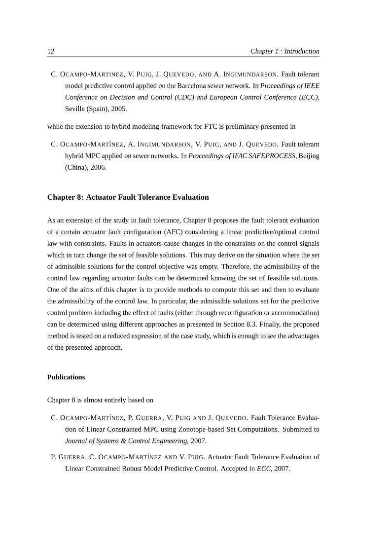
Rain gaugesRain can be considered the main external input. Hence, it is necessary to measure
the rain intensity in order to know the rain inflow. Rain intensity is measured using atip-
ping bucketrain-gauge, whose scheme is presented in Figure 2.5. This gauge technology
uses two smallbucketsmounted on a fulcrum (balanced like a see-saw). The tiny buckets
are manufactured with tight tolerances to ensure that they hold an exact amount of precip-
itation. The tipping bucket assembly is located underneaththe rain sewer, which funnels
the precipitation to the buckets. As rainfall fills the tiny bucket, it becomes overbalanced
and tips down, emptying itself as the other bucket pivots into place for the next reading.
2.1 : Sewer Networks: Definitions and Real-time Control 23
magnetreed switch
pivot
calibrationscrew
lock nutdrainhole
Figure 2.5: Rain measurement principle using a tipping bucket rain gauge.
The action of each tipping event triggers a small switch thatactivates the electronic cir-
cuitry to transmit the count to the indoor console, recording the event as an amount of
rainfall. Once the rain intensity is determined, the rain inflow can be computed using the
procedure proposed and explained in Chapter 3.
Limnimeters These devices measure the sewage level within the sewers. They are located on
strategy points of the network and their given information is related to the water volume
and flow by means of Manning formula, see Chapter 3. They are mainly used in points
where the sewer slope allows the water flow by gravity.
Velocity sensorsAccording to the geometry and topology of the considered sewer, flow infor-
mation can be inaccurate due to the level measurements. Then, these sensors are used
to measure the sewage velocity in an specific place of the sewer network. Using this in-
formation, the sewage flow can be computed in a more accurate manner. This fact for
instance avoids situations where the sewer slope is almost null, and despite the water flow
exists, the level of the water remains constant.
Radars An alternative way to measure rain intensity is usingweather radars. The weather
radar is an instrument used to obtain a detailed descriptionof the spatial and temporal
rainfall field. This information is needed to model in the hydrologically sense a certain

24 Chapter 2 : Background
Figure 2.6: Typical pumping station for reservoir. Taken from [CLA05].
region with sufficient resolution. However, such devices are complex instruments. They
measure a property of the rainfall drops. This property is related to the portion of the
power of the beam put out by the radar and that returns to it once the beam has hit its target.
This property, known as the rainfall reflectivity, is indirectly related to the rainfall intensity
(through the raindrop sizes distribution). It is also indirectly related to the intensity of the
rainfall that reaches the ground [GRA07].
Pumping Stations
Once a rain episode has finished, the tanks are drained towards the treatment plant. For this
procedure two elements can be needed: a retention gate and a pumping station. About first
element, some ideas have been presented beforehand. Pumping stations are needed to take out
the water that can not get out by gravity. Hence, these pumping stations are also manipulated,
allowing the flow control downstream. Figure 2.6 shows a typical pumping station for a sewer
network.

2.1 : Sewer Networks: Definitions and Real-time Control 25
Figure 2.7: View of the wastewater treatment plan of Columbia, Missouri(USA). Taken fromhttp://www.gocolumbiamo.com/.
Treatment Elements
This element consists in plants where, through physical-chemical and biological processes, or-
ganic matter, bacteria, viruses and solids are removed fromwastewaters before they are dis-
charged in rivers, lakes and seas. It receives all the water that has got into the sewer network
and has not got out through the overflows. Nowadays the inclusion of such elements within
the sewer networks is of great significance in order to preserve the ecosystem and maintain the
environmental balance inside the water cycle. In this sense, the separation of the storm sewers
from waste sewers would be a great strategy because the huge water inflow during a rainstorm
can overwhelm the treatment plant, resulting in untreated sewage being discharged into the en-
vironment. In this sense, some cities have dealt with this aspect by adding large storage tanks
or ponds to hold the water until it can be treated. Another wayto deal with this aspect consists
in design a suitable control strategy which prevents all type of pollution and Combined Sewage
Overflow (CSO) in the sewer network and then the damage to the environment. Figure 2.7
presents a picture of an important treatment plant located in Columbia, Missouri (USA).

26 Chapter 2 : Background
2.1.2 RTC of Sewage Systems
This section explores the contributions reported in the literature about the real-time control of
sewer networks. However, this literature exploration alsotakes into account modeling aspects
of sewage systems due to the close relation between modelingand control for thee particular
systems. Real-time sewer network control systems play an important role in meeting increas-
ingly restrictive environmental regulations to reduce release of untreated waste or CSO to the
environment. Reduction of CSO often requires major investments in infrastructure within city
limits and thus any improvement in efficient use of existing infrastructure, for example by im-
proved control, is of interest. The advantage of sewer network control has been demonstrated
by a number of researchers in the last decades, see [GR94], [PMLC96], [Mar99], [PCL+05],
[MP05]. A common control strategy to deal with urban drainage systems is Model Predictive
Control (MPC), see [GR94], [PPC+01] [MP05]. This fact is because the urban drainage control
problem is often multi-input, multi-output and the goal consists in using existing infrastructures
to their limits, characteristics that make MPC specially suitable with its inherent capacity to deal
with constraints.
A very important aspect on sewer networks is their modeling.Several modeling approaches
have been presented in the literature about sewer networks [Erm99], [Mar99], [DMDV01],
[MP05]. Specifically and due to its complex nature, several hydrological models have been
proposed [PMLC96], [ZHM01]. Sewer networks are systems with complex dynamics since wa-
ter flows through sewer in open channels. As will be discussedlater, flow in open canals are
described by Saint-Vennant’s partial differential equations that can be used to perform simula-
tion studies but are highly complex to solve in real-time. For the purpose of control, modeling
techniques have been presented that deal with sewer networks, see [DMDV01], [OMIPQ06].
However, when an implementation of a real-time control (RTC) strategy is implemented, the
complexity of the models could be an important problem because it implies higher computation
times and difficulties when a control sequence for a desired performance is computed [ZHM01],
[MP05]. This problem is also consequence of the high model dimension, proper characteristic
of the large-scale systems. Often the purpose of the model isto perform simulation studies and
they range from highly complex partial differential equations to simpler conceptual models.
In an early reference on MPC ([GR94]), a linear model of a sewer network was used for
prediction. Good performance of identified linear models insimulation of flow in urban drainage
networks with rain measurements as input has also been reported in [PLM99]. The use of
nonlinear models for predictive control of urban drainage systems has also been reported, see

2.1 : Sewer Networks: Definitions and Real-time Control 27
[RL95], [MP98].
Improvements in prediction achieved by using nonlinear models need to be compared to
the uncertainty introduced due to the error in predicting the rain over the horizon. Short term
rain prediction or nowcasting is an active field of research,see [SA00]. With a combination of
radar, rain gauge measurements and advanced data processing, prediction of rain has improved
greatly lately and the potential for the use in predictive control of urban drainage systems has
been pointed out in [YTJC99].
Then, an operational model of an urban drainage system wouldbe a set of equations which
provide a fast approximate evaluation of the hydrological variables of the network and their re-
sponse to control actions on the gates. In [RL95], nonlinearmodel predictive control (NMPC)
was implemented over a large-scale system with 26 states and10 manipulated inputs. It was
shown that a complex nonlinear model is always better but differences with linear MPC may
be too small to justify the NMPC effort. [MP97] justifies the use of simpler models for
optimization-based control of sewer networks due to
• the model inaccuracies impact is reduced solving the control problem iteratively and up-
dating inflow predictions and initial conditions, and
• the details of local elements and catchments are consideredin local control loops.
About control strategies, extensive research has been carried out on RTC of urban drainage
systems. Comprehensive reviews that include a discussion of some existing implementations are
given by [SAN+96] and its cited references, while practical issues are discussed by [SBB02],
among others. The common idea is the use of optimization techniques to improve the system
performance trying to avoid the street flooding, prevent theCSO discharges, minimize the pollu-
tion, get uniform the utilization of sewer system storage capacity and, in most of cases, minimize
the functioning costs, among another objectives [Erm99], [Wey02], [STJB02], [SCC+04]. In
this way, [GR94] proposed the implementation of model MPC over the Seattle urban drainage
system. In this work, authors organized the fundamental ideas about the use of these techniques
in sewer networks: definition of appropriate cost functions, creation and maintenance of models
and use of the prediction for minimizing the uncertainty effect of the rain estimation, aspect
that, in these systems is crucial for the right operation in closed-loop. Their results confirm the
effectiveness of the control law over large-scale systems relative to the used automatic controls
in that moment, which were based on heuristics.
Years later, [MP97] proposed the application of optimal control retaking the hierarchical

28 Chapter 2 : Background
control philosophy [Pap85]. This philosophy suggests thata RTC structure that combines high
efficiency and low implementation cost would have three layers:
• a adaptation layer, where the inflow prediction (rain) and state estimation in real-time is
done,
• a optimization layer, which is responsible of the global control and the reference trajecto-
ries computation, and
• a decentralized control layer, which is responsible of the control trajectories realization.
A similar idea of hierarchical control for RTC can be found in[SCC+04]. In [MP01], the
authors combine the work presented in [MP97] with the receding horizon philosophy, that is,
optimal control in finite horizon and prediction in a slidingtime window. [DMV04] implements
the global control level introduced in Figure 1.3 within theframework of predictive control
for minimizing the overflow volumes from combined sewers during rainfalls on the urban area
drained by the Marigot interceptor in Laval, Canada. The results have shown that allowing
surcharged flows in the interceptor during rainfalls leads to important decreases in overflow
volumes.
Although the application of optimization methods, and, more generally, the development of
control procedures, usually aims to determining the optimal (best possible) control action under
the given conditions, a suboptimal control decision is sometimes often enough for RTC (as long
as it can be ensured that this decision does not lead to a performance of the system worse than
the no-control scenario). However, under specific model conditions and for MPC strategies, it
could be ensured that the best possible solution is obtained.
2.2 MPC and Hybrid Systems
2.2.1 MPC Strategy Description
Model predictive control (MPC), alsoreferred as model based predictive control, receding hori-
zon controlor moving horizon optimal control, is one of the few advanced methodologies which
has significant impact on industrial control engineering. MPC is being applied in process in-
dustry because it can handle multivariable control problems in a natural form, it can take into

2.2 : MPC and Hybrid Systems 29
account actuator limitations and it allows constraints consideration. Predictive Control methods
are developed around certain common ideas, which are basically [Mac02], [GSdD05]:
• The explicit use of a model in order to predict the process output in a time horizon.
• The obtaining of a control sequence which minimizes a cost (objective) function.
• The application of the first control signal from the computedsequence and the displace-
ment of the horizon towards the future.
MPC as a wide field of control methods is developed around a setof basic elements in com-
mon. Its parameters can be modified giving rise to different algorithms. These main elements
can be outlined as:
• Prediction model, which should capture all process dynamics and allows to predict the
future behavior of the system.
• Objective (cost) function, which is, in general form, the element that penalizes derivations
of the predicted controller outputs from a reference trajectory. It represents a performance
index of the system studied.
• Control signal computation.
This control strategy presents important advantages over other control methods. Some of
these advantages are outlined below [Bor00].
• It is very easy to use for people without deep knowledge in control. Its concepts are very
intuitive and the tuning is relatively simple.
• Can be used to control a wide type of processes, including simple dynamics towards
systems with big delays, unstable and nonminimum phase systems.
• It is very useful for multivariable systems.
• It has inherently the delay compensation.
• It allows the use of constraints, which can be added during the design process.
However, it also has some disadvantages such as the high computational cost in the control
law obtaining process. But the main problem of this strategylies on the dependence of a accurate

30 Chapter 2 : Background
system model. The design algorithm is based on the previous knowledge of the system behavior
so the performance is related to the quality of the plant representation.
MPC Formulation
In most of the cases presented in the research literature, the MPC formulation is expressed in
state space. However, in order to present a generic and simple representation of the strategy, let
xk+1 = g(xk, uk) (2.1)
be the mapping of statesxk ∈ X ⊆ Rn and control signalsuk ∈ U ⊆ Rm for a given system,
whereg : Rn ×Rm → Rn is the arbitrary system state function andk ∈ Z+. Let
uk(xk) ,(u0|k, u1|k, . . . , uHp−1|k
)∈ U
Hp (2.2)
be the input sequence over a fixed time horizonHp. Moreover, theadmissible input sequence
with respect to the statexk ∈ X is defined by
UHp(xk) ,uk ∈ U
Hp |xk ∈ XHp, (2.3)
where
xk(xk,uk) ,(x1|k, x2|k, . . . , xHp|k
)∈ X
Hp (2.4)
corresponds to the state sequence generated applying the input sequence (2.2) to the system (2.1)
from initial statex0|k , xk, wherexk is the measurement or the estimation of the current state.
Hence, the receding horizon approach is based on the solution of the open-loop optimization
problem (OOP) [BM99b]:
minuk∈ UHp
J (uk, xk,Hp) (2.5a)
subject to
H1uk ≤ b1 (2.5b)
G2xk +H2uk ≤ b2 (2.5c)
whereJ(·) : Xf (Hp) 7→ R+ is the cost function with domain in theset of feasible states
Xf (Hp) ⊆ X [LHWB06], Hp denotes theprediction horizonor output horizonandG2,Hi and
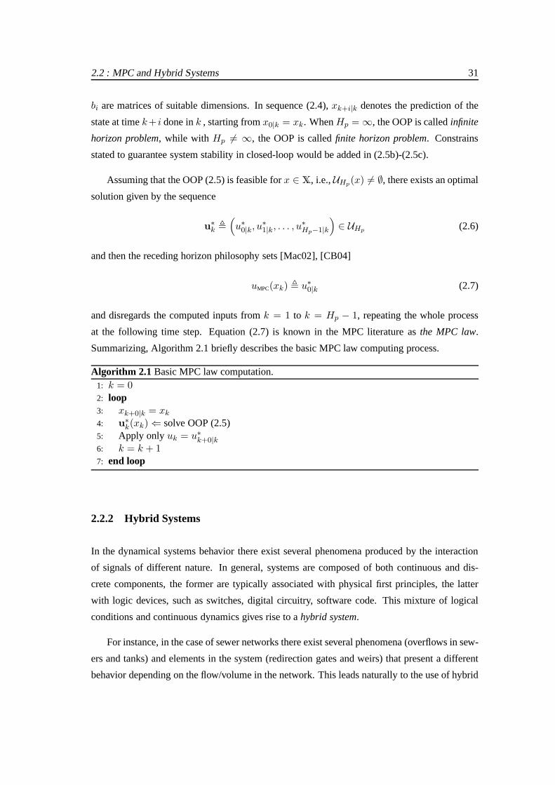
2.2 : MPC and Hybrid Systems 31
bi are matrices of suitable dimensions. In sequence (2.4),xk+i|k denotes the prediction of the
state at timek+ i done ink , starting fromx0|k = xk. WhenHp =∞, the OOP is calledinfinite
horizon problem, while with Hp 6= ∞, the OOP is calledfinite horizon problem. Constrains
stated to guarantee system stability in closed-loop would be added in (2.5b)-(2.5c).
Assuming that the OOP (2.5) is feasible forx ∈ X, i.e.,UHp(x) 6= ∅, there exists an optimal
solution given by the sequence
u∗k ,
(u∗0|k, u
∗1|k, . . . , u
∗Hp−1|k
)∈ UHp (2.6)
and then the receding horizon philosophy sets [Mac02], [CB04]
uMPC(xk) , u∗0|k (2.7)
and disregards the computed inputs fromk = 1 to k = Hp − 1, repeating the whole process
at the following time step. Equation (2.7) is known in the MPCliterature asthe MPC law.
Summarizing, Algorithm 2.1 briefly describes the basic MPC law computing process.
Algorithm 2.1 Basic MPC law computation.1: k = 02: loop3: xk+0|k = xk
4: u∗k(xk)⇐ solve OOP (2.5)
5: Apply only uk = u∗k+0|k6: k = k + 17: end loop
2.2.2 Hybrid Systems
In the dynamical systems behavior there exist several phenomena produced by the interaction
of signals of different nature. In general, systems are composed of both continuous and dis-
crete components, the former are typically associated withphysical first principles, the latter
with logic devices, such as switches, digital circuitry, software code. This mixture of logical
conditions and continuous dynamics gives rise to ahybrid system.
For instance, in the case of sewer networks there exist several phenomena (overflows in sew-
ers and tanks) and elements in the system (redirection gatesand weirs) that present a different
behavior depending on the flow/volume in the network. This leads naturally to the use of hybrid

32 Chapter 2 : Background
models in order to describe such behaviors. The hybrid models considered here belong to the
class of discrete-time linear hybrid systems. The condition of discrete-time avoids certain math-
ematical problems (like Zeno behavior, see [HLMR02], [AS05]) and allows to derive models
for which analysis and optimal/predictive control problems can be posed.
Mixed Logical Dynamical Systems
TheMixed Logical Dynamical(MLD) modeling framework, introduced in [BM99a], is a way,
among others, that allows one to represent hybrid systems, which can be described by interde-
pendent physical laws, logical rules and operating constraints. MLD models have recently been
shown to be equivalent to representations of hybrid systemssuch asLinear Complementarity
(LC) systems,Min-Max-Plus Scaling(MMPS) systems andPiecewise Affine(PWA) systems,
among others, under mild conditions, see [HDB01]. MLD systems are described by linear dy-
namic equations subject to linear mixed-integer inequalities, i.e., inequalities involving both
continuous and binary (or logical, or 0-1) variables. Theseinclude physical/discrete states,
continuous/integer inputs, and continuous/binary auxiliary variables. The ability to include
constraints, constraint prioritization and heuristics are powerful features of the MLD model-
ing framework. The general MLD form is [BM99a]:
xk+1 = Axk +B1 uk +B2 δk +B3 zk (2.8a)
yk = Cxk +D1 uk +D2 δk +D3 zk (2.8b)
E2 δk + E3 zk ≤ E1 uk + E4 xk + E5 (2.8c)
where the meaning of the variables is the following:
• x are the continuous and binary states:
x =
[xc
xℓ
], xc ∈ X ⊆ R
nc, xℓ ∈ 0, 1nℓ (2.9)
• y are the continuous and binary outputs:
y =
[yc
yℓ
], yc ∈ Y ⊆ R
pc, yℓ ∈ 0, 1pℓ (2.10)

2.2 : MPC and Hybrid Systems 33
• u are the continuous and binary inputs:
u =
[uc
uℓ
], uc ∈ U ⊆ R
mc , uℓ ∈ 0, 1mℓ (2.11)
• Auxiliary binary variables:δ ∈ 0, 1rℓ
• Auxiliary continuous variables:z ∈ Rrc.
Notice that by removing (2.8c) and by settingδ andz to zero, (2.8a) and (2.8b) reduce to an
unconstrained linear discrete time system in state space. The variablesδ andz are introduced
when translating logic propositions into linear inequalities. All constraints are summarized in
the inequality (2.8c).
The transformation of certain hybrid system descriptions into the MLD form requires the
application of a set of given rules. To avoid the tedious procedure of deriving the MLD form by
hand, a compiler was developed in [TB04] to generate matricesA, Bi, C, Di andEi in (2.8)
through the specification language HYSDEL (HYbrid System DEscription Language).
2.2.3 MPC Problem on Hybrid Systems
Different methods for the analysis and design of hybrid systems have been proposed in the
literature during the last few years [BM99a], [LTS99], [BZ00]. The implementation of these
methods are related in a straightforward manner to the hybrid system representation. One of the
most studied methods involves the class of optimal controllers, which may use the MLD form in
order to compute the corresponding control law according tothe system performance objectives.
The formulation of the optimization problem in Hybrid MPC (HMPC) follows the approach in
standard MPC design, see [Mac02]. The desired performance indexes are expressed as affine
functions of the control variables, initial states and known disturbances. However, due to the
presence of logical variables, the resulting optimizationproblem is amixed integer quadraticor
linear program(MIQP or MILP, respectively). The control law obtained in this way is referred
to asmixed integer predictive control(MIPC).
In general, the MIPC structure is defined by the OOP (2.5) described as beforehand but
including the logical dynamics part. Hence, the OOP considering the hybrid systems framework
is presented as follows. Assume that the hybrid system output should track a reference signalyr
andxr, ur, zr are desired references for the states, inputs and auxiliaryvariables, respectively.

34 Chapter 2 : Background
For a fixed prediction horizonHp ∈ Z≥1, the input sequence (2.2) is applied to the system (2.8),
resulting the sequences (2.4) and
∆k(xk,uk) ,(δ0|k, δ1|k, . . . , δHp−1|k
)∈ 0, 1rℓ×Hp (2.12)
zk(xk,uk) ,(z0|k, z1|k, . . . , zHp − 1|k
)∈ R
rc×Hp (2.13)
under the same conditions as in problem (2.5).
Hence, the OOP for hybrid systems is now defined as:
minuk∈ UHp,∆k,zk
J (uk(xk),∆k, zk, xk) ,∥∥Qxf
(xHp|k − xf
)∥∥p
+
Hp−1∑
i=1
∥∥Qx
(xk+i|k − xr
)∥∥p+
Hp−1∑
i=0
∥∥Qu
(uk+i|k − ur
)∥∥p
+
Hp−1∑
i=0
(∥∥Qz
(zk+i|k − zr
)∥∥p+∥∥Qy
(yk+i|k − yr
)∥∥p
)(2.14a)
subject to
xk+i+1|k = Axk+i|k +B1uk+i|k +B2δk+i|k +B3zk+i|k
yk+i|k = Cxk+i|k +D1uk+i|k +D2δk+i|k +D3zk+i|k
E2δk+i|k + E3zk+i|k ≤ E1uk+i|k +E4xk+i|k + E5
xf = xrHp|k
(2.14b)
for i = 0, . . . ,Hp−1, wherexf corresponds to the final desired value for the state variableover
Hp andp is related to the selected norm (1-norm, quadratic norm or infinity norm). Qxf, Qx,
Qu, Qδ, Qz andQy are the weight matrices of suitable dimensions, which fulfill the following
conditions:
Qxf ,x,u = QTxf ,x,u ≻ 0, Qδ,z,y = QT
δ,z,y 0 (p = 2)
Qxf, Qx, Qu, Qδ, Qz , Qy nonsingular (p = 1, p =∞)
(2.15)
Assuming that the MIPC problem related to the OOP (2.14) is feasible forx ∈ X, there
exists an optimal solution given now by the sequence
(u∗0|k, u
∗1|k, · · · , u∗Hp−1|k, δ
∗0|k, δ
∗1k, · · · , δ∗Hp−1|k, z
∗0|k, z
∗1|k, · · · , z∗Hp−1|k
)
which, applying the receding horizon strategy, yields the MPC law in (2.7). Notice that the
described procedure corresponds to the extension of MPC formulation in Section 2.2.1 over
hybrid systems but the solution is obtained solving the OOP (2.14).

2.3 : Fault Tolerance Mechanisms 35
Some theoretical aspects about control of hybrid systems can be discussed and they have
been a research topic during the last few years. For instance, notice thatHp should be finite.
Infinite horizon formulations are not pragmatic neither theoretically nor in practical implemen-
tation. The approximation ofHp as large as possible implies a great amount of logical variables
within the MIPC problem, what yields an almost impossible computation treatment [BM99a].
The assumptionHp → ∞ is already worse in the case of large scale systems. On the other
hand, the constraintxf = xrHp|k, related to the final state within the MIPC problem (2.14),
can be relaxed asxHp|k ∈ XT ⊆ X, whereXT is defined as thetarget state set[LHWB06].
According to this assumption, the sequenceUHp(x(k)) in (2.3) is redefined with respect toXT
as
UHp(xk) , uk ∈ UHp |xk ∈ X
Hp , xHp|k ∈ XT . (2.16)
All concepts, formulations and definitions presented so farare used in next chapters to
present the MPC formulation not only for linear but also for hybrid systems. Chapters 4 and 8
considers the definition of a OOP where the model is purely linear while Chapters 5, 6 and 7
consider the OOP for an hybrid system.
2.3 Fault Tolerance Mechanisms
The aim of RTC on sewer networks is to improve its performancein extreme meteorological
conditions. Under these conditions, it is very likely that afault occurs in any constitutive element
of the network, what leads to losing the control effectiveness, degrading the performance and
even causing dangerous situations such as severe flooding orpollution. Then, it is extremely
needed to have fault tolerance mechanisms that reduce the faults effect, ensuring at least the
partial fulfilling of the control objectives.
Fault Tolerant Control(FTC) is a new idea recently introduced in the research literature
[Pat97] which allows to have a control loop that fulfills its objectives (maybe with a possible
degradation) when faults in components of the system (instrumentation, actuators and/or plant)
appear. A control loop could be considered fault tolerant ifthere exist:
• Adaptation strategies of the control law included in the closed-loop.
• Mechanisms that introduce redundancy in sensors and/or actuators.
Figure 2.8 presents a possible classification of the fault tolerance mechanisms considered in

36 Chapter 2 : Background
FaultTolerance
Mechanisms
FTCStrategies
FaultyElement
Reposition
ActiveFTC
PassiveFTC
Accommodation
ReconfigurationOn-line
On-line
Off-line
Off-line
PhysicalRedundancy
AnalyticalRedundancy
Sensor
Sensor
Actuator
Actuator
Figure 2.8: Classification of Fault Tolerance Mechanisms
this section.
2.3.1 Fault Tolerance by Adaptation of the Control Strategy
From the point of view of the control strategies, the literature considers two main groups: the
activeand thepassivetechniques. The passive techniques are control laws that take into ac-
count the fault appearance as a system perturbation. Thus, within certain margins, the control
law has inherent fault tolerant capabilities, allowing thesystem to cope with the fault presence.
In [CPC98], [LLL00], [QIYS01], [LWY02] and [QIYS03], amongmany others, complete de-
scriptions of passive FTC techniques can be found.
On the other hand, the active fault tolerant control techniques consist in adapting the con-
trol law using the information given by the FDI block. With this information, some automatic
adjustments are done trying to reach the control objectives.
Scheme of Figure 2.9 proposes a particular architecture of an active FTC loop introduced
by [Bla99], which contains three design levels: thecontrol loop(level 1), theFault Diagnosis
and Isolation(FDI) system (level 2) and thesupervisor system(level 3), which closes the outer

2.3 : Fault Tolerance Mechanisms 37
loop and adds the fault tolerance capabilities.
The feedback control loop shown in Figure 2.9 is composed by acontrol law, anactuator
or set of actuators, theplant and asensoror set/array of sensors. In parallel with sensor and
actuator blocks, there exist other hardware or software blocks used to provideredundancyin
the signal measurement as in the application of the control action. This redundancy could be
introduced in physical form (redundant sensors or actuators) or in analytical form (through
mathematical models). From the input and output signals of sensors, actuators and the plant, FDI
system detects and isolates the faults, quantifies their magnitude and identifies the specific faulty
elements, if possible. Next, FDI system sends this information to theAutomatic Supervisor
(AS), which takes the corresponding decisions in order to maintain the control loop operative in
spite of the fault.
Notice that AS block is a discrete event system while the supervised system is defined in
continuous time. The information exchange between both systems is done through the FDI
block. Due to the whole system has a mixed nature, its corresponding analysis and design
could be done using thehybrid systems theory(see [CLO95], [BM99a], [AHS01], [MBB03],
among many others), this being an open area that is been currently explored and developed in
the research literature. In this way, this idea is further developed and discussed in Chapter 7.
Once the AS block receives the information from the FDI module, it evaluates the admissi-
bility of the system performance taking into account the fault presence. To do this, AS considers
whether the control objectives: (i) are fulfilled acceptinga certain degradation level (region of
degraded performance), or (ii) are not fulfilled but there isstill the possibility of activating cor-
rective actions (region of unacceptable performance). Otherwise, the process should be stopped
(region of danger). Figure 2.10 shows the above mentioned regions of operation for a two-states
system. Chapter 8 of this thesis presents a methodology thathelps on doing the the admissibility
task.
Accommodation and Reconfiguration Strategies
In order to understand the operation of the different strategies within the active FTC philosophy,
the standard feedback control problem is defined by [BKLS03]:
〈O,C(θ),U〉, (2.17)

38 Chapter 2 : Background
AU
TO
MA
TIC
SU
PE
RV
ISO
R
FD
IBL
OC
KP
LA
NT
PL
AN
T
MO
DE
L
MO
DE
VIR
TU
AL
VIR
TU
AL
AC
TU
AT
OR
AC
TU
AT
OR
PH
YS
ICA
LP
HY
SIC
AL
RE
DU
ND
AN
CY
RE
DU
ND
AN
CY
OP
ER
AT
ION
CO
NT
RO
LL
AW
SE
NS
OR
SE
NS
OR
HU
MA
NS
UP
ER
VIS
OR S
ET
PO
INT
LEVEL 3 LEVEL 2 LEVEL 1
ua
y pu
cu
a
y s
y s
y L
Figure 2.9: Proposed architecture for a fault tolerant control system.
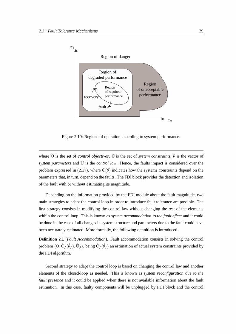
2.3 : Fault Tolerance Mechanisms 39
x1
Region of danger
Region ofdegraded performance
Regionof requiredperformancerecovery
fault
Regionof unacceptable
performance
x2
Figure 2.10: Regions of operation according to system performance.
whereO is the set ofcontrol objectives, C is the set ofsystem constraints, θ is the vector of
system parametersandU is thecontrol law. Hence, the faults impact is considered over the
problem expressed in (2.17), whereC(θ) indicates how the systems constraints depend on the
parameters that, in turn, depend on the faults. The FDI blockprovides the detection and isolation
of the fault with or without estimating its magnitude.
Depending on the information provided by the FDI module about the fault magnitude, two
main strategies to adapt the control loop in order to introduce fault tolerance are possible. The
first strategy consists in modifying the control law withoutchanging the rest of the elements
within the control loop. This is known assystem accommodation to the fault effectand it could
be done in the case of all changes in system structure and parameters due to the fault could have
been accurately estimated. More formally, the following definition is introduced.
Definition 2.1 (Fault Accommodation). Fault accommodation consists in solving the control
problem〈O, Cf (θf ), Uf 〉, beingCf (θf ) an estimation of actual system constraints provided by
the FDI algorithm.
Second strategy to adapt the control loop is based on changing the control law and another
elements of the closed-loop as needed. This is known assystem reconfiguration due to the
fault presenceand it could be applied when there is not available information about the fault
estimation. In this case, faulty components will be unplugged by FDI block and the control

40 Chapter 2 : Background
objective will try to be reached using the non faulty components. Then, a formal definition is
given as follows.
Definition 2.2 (System Reconfiguration). System reconfiguration due to the fault presence con-
sists in finding a new set of constraintsCf (θf ) such that the control problem〈O,Cf (θf ),Uf 〉can be solved. Then, this solution is found and applied.
On-line/Off-line Control Law Adaptation
Once the adaptation approach of the control law is selected,there are two main ways of im-
plementation within the control loop. The basic differencebetween them is that in one case
(off-line adaptation), the control law parameterized withrespect to the faults is pre-computed
off-line while in the other case (on-line adaptation), the control law is recomputed on-line taking
into account the faults. These ways are:
Off-line Adaptation (Also known as adaptation using precalculated controller). In this case,
the control law could be written asUf = U(f), wheref corresponds to the determined
fault. Thus, within the FTC architecture there exists a block used to determine the oper-
ation mode of the system once the fault occurs, what allows tocomputeUf (see Figure
2.11(a)). A possible characterization of the control laws on this framework according to
the plant nature (mathematical model) is given in [The03] asfollows:
• Control Laws for LTI Models: techniques based on LTI system models, such as
Model Matching[Kun92], Model Following[Jia94],LQRandEigenstructure assig-
ment[Jia94] [ZJ02], among others.
• Control Laws for a LTI Models family: techniques based on LTI models obtained
by linearization around a set of equilibrium points, covering a certain portion of the
whole state space. Some examples areMulti-models, Gain-Schedulingand LPV,
among others.
• Control Laws for Nonlinear Models: techniques based on nonlinear mathematical
model of the plant. In this case,soft-computingtechniques to design the controller
are usually implemented. Examples of these laws are Fuzzy Control, Neural Con-
trol, Neuro-Fuzzy Control, among others [DP01].
On-line Adaptation (Also known as adaptation by using an on-line computed controller). In
this case, the control lawU is obtained on-line from an estimation of the actual system re-
strictionsCf (θf ) once the fault occurs. Figure 2.11(b) shows the basic operation scheme

2.3 : Fault Tolerance Mechanisms 41
for this case. Also, for the estimation of the fault effect onthe system constraints, two
alternatives exist:
• Off-line estimation: The fault effect over the system constraints has been considered
off-line. This fact allows to express such constraints in function of the fault and
to change the control law according to the fault informationprovided by the FDI
module. In this way, the controller is always recomputed taking into account the
fault effect in the system constraints. Examples of controltechniques of this group
are theModel Predictive Control(MPC) [MR93], [ML01] andStatic Feedback Lin-
earization[ZJ03].
• On-line estimation: The fault effect over the system constraints is computed on-line
so the controller will change on-line as well. Examples of control techniques of
this group areAdaptive Control[IS95], [DP02],Dynamic Feedback Linearization
[ZJ03] andDual Predictive Control[VX98].
2.3.2 Fault Tolerance by Reposition of Sensors and/or Actuators
Serious faults in sensors or actuators break the control loop. In order to maintain the system in
operation, some redundancy should be present in such a way that a new set of sensors (plant
inputs) or actuators (plant outputs) is used. To do this, an accommodation block is implemented
to work together with the plant and the other non-faulty elements. The main objective consists
in having a closed-loop with almost the same performance of the non faulty closed-loop trying
to maintain the desired control objectives.
The required redundancy for sensors/actuators fault tolerance can be achieved either using
physical redundancy (also calledhardware redundancy) or using analytical redundancy (also
known assoftware redundancyor redundancy by virtual element).
Fault Tolerance in Sensors
In the case of sensors, the physical redundancy consists in having an odd number of measure-
ment elements which outputs are multiplexed in a decision block. Such block gives the correct
measurement from the determination of the more common signal value of all multiplexed sig-
nals. On the other hand, tolerance mechanism by using analytical redundancy consists in using
an observer in order to rebuild the system measurements fromother existing sensors. For this

42 Chapter 2 : Background
ControlControl
mea
sure
men
ts
signals
signalsactions
Event: Fault
REALPLANT CONTROL
OFFLINE
ESTIMATOR
SENSORS
ACTUATORS
FDI BLOCK
AUXILIARACTUATORS
(a) Off-line
ControlControl
mea
sure
men
ts
modelaccom
modation
signals
signalsactions
Event: Fault
REALPLANT
ONLINECONTROL
ESTIMATOR
SENSORS
ACTUATORS
FDI BLOCK
AUXILIARACTUATORS
HYBRIDMODEL
(b) On-line
Figure 2.11: Conceptual schemes for FTC law adaptation.

2.4 : Summary 43
reason, this technique is also knownvirtual or software sensor. The design of a sensors network
considering the criteria of fault tolerance, system observability, costs and robustness is nowa-
days an important subject of study in the literature [HSA00], [AHS01]. In [SHA04], estimations
of fault tolerance associated to the design of sensor networks is proposed. In this work, aspects
like reliability of a set of sensors, its fault tolerance capabilities and minimum number of re-
dundant sensors are evaluated. Applications of these mechanisms can be found in aeronautics
[LDC99], [HIM01], in AC systems [BPD99], among many others.
Fault Tolerance in Actuators
As in the case of sensors, the physical redundancy in actuators consists in having additional units
that can be multiplexed in a decision block by unplugging thefaulty actuator and connecting an
alternative non faulty.
On the other hand, in the case of a over-actuated system, somekind of physical redundancy
exists. This fact allows to adapt the control law (either through accommodation or reconfigura-
tion strategies)in order to find a suitable control actions for non-faulty actuators. In this way, the
control objectives can be fulfilled with an acceptable degradation level [DMHN99]. Thus, the
incorporation of new hardware to the closed-loop is avoided, which makes cheaper the imple-
mentation. For instance, in the case of large scale water systems where there are thousands of
actuators, this approach is suitable for achieving actuator fault tolerance (see Chapters 7 and 8).
From the theoretical point of view, analytical redundancy used to achieve actuator fault
tolerance has been recently proposed a dual strategy of the virtual sensor known asvirtual
actuator [LS03] but the proposal is currently limited to be treated and discussed only in the
field of the FTC analysis and design.
2.4 Summary
This chapter has presented the main aspects for each one of the constitutive topics related to
the thesis. First section has collected definitions, concepts and discussions from literature about
sewer networks and their constitutive elements. Moreover,a brief state of the art regarding real-
time control of such systems has been also outlined. In this part, references to actual research
state have been outlined and described.

44 Chapter 2 : Background
In the second section, MPC strategy, hybrid systems and the MPC formulation as RTC
control strategy on sewage systems have been presented and discussed.
Finally, the third section collects the main ideas about theexisting fault tolerance mecha-
nisms. In Chapter 3, sewer network elements presented in Section 2.1 are described using a
given mathematical modeling principles in order to obtain amodel of the case study considered
in this thesis. MPC formulations and concepts for linear systems are applied in Chapter 4 while
for hybrid systems are applied in Chapters 5, 6 and 7. Moreover, also in Chapter 7 and in Chap-
ter 8, descriptions and definitions about fault tolerance and FTC introduced in Section 2.3 are
considered and their application is discussed.

CHAPTER 3
PRINCIPLES OFMATHEMATICAL
MODELING ON SEWER NETWORKS
One of the most important stages on the RTC of sewer networks,and in general in the control
of dynamical systems, lies on the definition of the model for the considered system. Some
control techniques such as MPC are very dependent of this issue in order to obtain acceptable
performance and satisfactory results due to the accuracy ofthe open-loop model. This chapter
is focused on the determination of a control oriented sewer network model taking into account
the trade-off between model accuracy and model complexity [GR94]. Moreover, this chapter
proposes and describes a case study based on a real sewer network based on the Barcelona
urban drainage system. Using such case study, in subsequentchapters control strategies and
their associated advantages and problems are discussed notonly in nominal mode but also in
faulty mode.
3.1 Fundamentals of the Mathematical Model
The water flow in sewers is open-channel, i.e., the flow sharesa free surface with an empty
space above. The Saint-Venant equations1, based on physical principles of mass conservation
and energy, allow to describe accurately the flow in open-flowchannels as, for instance, the
1Adhemar Jean Claude Barre de Saint-Venant (1797 - 1886) was a mechanician who developed the one-dimensional unsteady open channel flow shallow water equations or Saint-Venant equations that are a fundamentalset of equations used in modern hydrological engineering.
45

46 Chapter 3 : Principles of Mathematical Modeling on Sewer Networks
sewer within a network [May04]. These equation in general form are expressed as:
∂qx,t
∂x+∂Ax,t
∂t= 0 (3.1a)
∂qx,t
∂t+
∂
∂x
(q2x,t
Ax,t
)+ gAx,t
∂Lx,t
∂x− gAx,t (I0 − If ) = 0 (3.1b)
whereqx,t is the flow (m3/ s),Ax,t is the cross-sectional area of the sewage flow (m2), t is the
time variable (s),x is the spatial variable measured in the direction and the sense of the water
flow (m), g is the gravity (m/ s2), I0 is the sewer slope (dimensionless),If is the friction slope
(dimensionless) andLx,t is the water level inside the sewer (m). This pair of partial-differential
equations constitutes a nonlinear hyperbolic system, thatfor an arbitrary geometry lacks on ana-
lytical solution. Notice that these equations get high detail level in the description of the system
behavior. However, such detail level is not useful for real-time control implementation due to
the complexity of obtaining the solution of (3.1) and the high computational cost associated
[Cro05].
Alternatively, several modeling techniques have been presented in the literature that deal
with real-time control of sewer networks, see [MP98], [Erm99], [DMDV01], [MP05], among
many others. The modeling approach used in this chapter is based on the proposal presented in
[GR94]. There, the sewer system was divided into connected subgroups of sewers and treated
as interconnectedvirtual tanks(see Figure 3.1). At any given time, the stored volumes represent
the amount of water inside the mains associated with the tankand are calculated on the basis
of area rainfall and flow exchanges between the interconnected virtual tanks. The volume is
calculated through the mass balance of the stored volume, the inflows and the outflow of the
tank and the input rain intensity.
Using the virtual tanks approach and the sewer network elements presented in Section 2.1,
the following elementary models are introduced:
Tanks (both virtual and real) The mass balance of the stored volume, the inflows and the out-
flow of the tank and the input rain intensity mentioned beforecan be written as the differ-
ence equation
vik+1 = vik + ∆tϕiSiPik + ∆t(qi
ink − qiout
k
), (3.2)
whereϕi is theground absorption coefficientof the i-th catchment,S is the surface area,
P is the rain intensity in each sample, with a sampling time∆t. qiink andqioutk are the

3.1 : Fundamentals of the Mathematical Model 47
Rain A Rain B
Rain D Rain E
Rain C
TANK A TANK B
TANK C
TANK D TANK E
Water leaks
Water leaksWater leaks
Water leaks
Water leaks
FLOW AC
FLOW B-C
FLOW C-D FLOW C-E
FLOW D FLOW E
Figure 3.1: Sewer network modeling by means ofvirtual tanks.
sum of inflows and outflows, respectively.Real retention tanks, which corresponds to the
sewer network reservoirs, are modeled in the same way but without the precipitation term.
The tanks are connected with flow paths or links which represents the main sewage pipes
between the tanks. The manipulated variables of the system,denoted asqui, are related
to the outflows from the control gates. The tank outflows are assumed to be proportional
to the tank volume (linear tank model approach), that is,
qioutk = βivik, (3.3)
whereβi (given in s−1) is defined as thevolume/flow conversion(VFC) coefficient as
suggested in [Sin88]. Notice that this relation can be made more accurate (but more
complex) if 3.3 is considered to be non-linear (non-linear tank model approach).
The limit on the range of real tanks is expressed as:
0 ≤ vik ≤ vi (3.4)
wherevi denotes the maximum volume capacity given in m3. As this constraint is phys-
ical, it is impossible to send more water to a real tank than itcan store. Notice that
reservoirs without overflow capability have been considered. The virtual tanks do not

48 Chapter 3 : Principles of Mathematical Modeling on Sewer Networks
have a physical limit on their capacity. When they rise abovea decided level an overflow
situation occurs. This represents the case when the level inthe sewers has reached a limit
so that an overflow situation can occur in the streets.
Gates In the case of a real tank, aretention gateis present to control the outflow. Virtual tank
outflows can not be closed but can be redirected usingredirection gates. The redirection
gates divert the flow from a nominal flow path which the flow follows if the redirection
gate is closed. This nominal flow is denoted asQi in the equation below, which expresses
mass conservation at the redirection gate:
qiink = Qik +
∑
j
qjuik, (3.5)
wherej is an index over all manipulated flowsqjui coming from the gate andqiin is the
flow coming to the gate. The flow path whichQi represents is assumed to have a cer-
tain capacity and when this capacity reaches its limit, an overflow situation occurs. This
flow limit will be denotedQi. WhenQi reaches its maximum capacity, two cases are
considered:
1. The water starts to flow on the streets, causing a flooding situation.
2. The water exits the sewer network and is considered lost tothe environment.
In the first case, the overflow water either follows the nominal flow path and ends up in
the same tank asQi or it is diverted to another virtual tank. Flow to the environment
physically represents the situation when the sewage ends upin a river, in the sea or in
another receiver environment. When using this modeling approach where the inherent
nonlinearities of the sewer network are simplified by assuming that only flow rates are
manipulated, physical restrictions need to be included as constraints on system variables.
For example, variablesqjui that determinate outflow from a tank can never be larger than
the outflow from the tank. This is expressed with the inequality
∑
j
qjuik≤ qiout
k = βivik. (3.6)
Usually the range of actuation is also limited so that the manipulated variable has to fulfill
qjui≤ qj
uik ≤ qjui , whereq
uidenotes the lower limit of manipulated flow andqui
denotes
its upper limit. Whenqjui
equals zero, this constraint is convex but if the lower boundis
larger than zero, constraint (3.6) has to be included in the range limitation. This leads to

3.2 : Calibration of the Model Parameters 49
the following non-convex inequality:
min(qjui, qi
outk −
∑
t6=j
qtuik
) ≤ qjuik≤ qj
ui(3.7)
The sum in the expression is calculated for all outflows related to tanki exceptj. A
further complexity is that whether the control signal is a inflow to a real tank that has hard
constraints on its capacity, then the situation can occur that this lower limit is also limited
by this maximum capacity and the outflow from the real tank.
Weirs (Nodes) This elements includes in the model of a sewer network the switching behavior
since describes the situation when sewage flow has a restriction due to sewer capacity
and “jumps” trying to find another path. According to discussion in Section 2.1, these
elements can be classified assplitting nodesandmerging nodes. The first can be treated
considering a constant partition of the flow in predefined portions according to the topo-
logical design characteristics. Merging nodes exhibits a switching behavior. In the case
of a set ofn inflows qi, with i = 1, 2, . . . , n, an outflowqout and a maximum outflow
capacityqout, the expressions for this element under the aforementionedconditions are:
qin =
n∑
i=0
qi (3.8a)
qout = minqin, qout (3.8b)
qover = max0, qin − qout (3.8c)
whereqover corresponds to the node overflow. Notice that these expressions define a
nonlinear model of the element with all their possible implications.
Remark3.1. Overflows in sewers (links) follow almost the same description as the nodes since
the overflow phenomenon in these elements can be considered as the case of a merging node
having a maximum capacity in the nominal outflow path relatedto the flow capacity of the
sewer.
3.2 Calibration of the Model Parameters
In order to estimate the parameters of virtual tanks from real data, measurements coming from
sensors are available. Water level measurements in sewers are taken using ultrasonic limnime-
ters. Notice that the sewer level is measured instead of the flow. This is because the level sensors

50 Chapter 3 : Principles of Mathematical Modeling on Sewer Networks
do not have contact with the water flow, what prevents problems such as wrong measurements
caused by sensor faults. From these level measurements, theflow entering and exiting each vir-
tual tank can be estimated assuming steady-uniform flow and using Manning formula2 [May04]
q = vSw, (3.9)
whereSw is the wetted surface that depends on the cross-sectional sewer areaA and water
levelL within the sewer. The dependence ofA andL onx andt are omitted for compactness.
Moreover,v is the water velocity computed according to the parameters relation
v =Kn
nR
2/3h I
1/20 , (3.10)
whereKn is a constant whose value depends on the measurement units used in the equation,n
is the Manning coefficient of roughness which depends on flow resistance offered by the sewer
material,Rh is the hydrological radius defined as the relation of the cross sectional area of flow
and the wetted perimeterp asRh = A/P , andI0 is the sewer slope. For a given geometry of the
sewer cross-section, wetted perimeter and hydrological radius can be expressed in function of
the sewer levelL. For instance, given a rectangular cross-section of widthb, the wetted surface
Sw is bL, p is b+ 2L and the hydrological radius is given byRh = bLb+2L .
Using the rain intensitiesPi and the stated input/output flows, by combining (3.2) and (3.3),
the following input/ouput equation in function of the flow insewers and rain intensity in catch-
ments can be obtained and expressed as:
qioutk+1 = a qi
outk + b1 Pik + b2 qi
ink , (3.11)
wherea = (1− βi∆t), b1 = βi∆tϕiSi andb2 = βi∆t. Figure 3.2 represents this equation and
the interaction of all described parameters and measurements.
Equation (3.11) is linear in the parameters, what allows to estimate them using classical
parameter estimation methods based onleast-squares algorithm[Lju99]. Hence, the parameter
associated to the ground absorption coefficient is estimated as:
ϕi =b1b2Si
(3.12)
2The Manning formula is an empirical formula for open channelflow, or flow driven by gravity. It was devel-oped by the French engineerRobert Manningand proposed on 1891 in the Transactions of the Institution of CivilEngineers (Ireland).

3.3 : Case Study Description 51
Linear Tank
Si
Rain
LevelSensor
LevelSensor
Rain-gauge
qini
qouti
Figure 3.2: Scheme of an individual virtual tank and its parameters andmeasurements.
and the VFC coefficient is estimated as:
βi =b2∆t
(3.13)
for the i-th catchment.
Ground absorption and volume/flow conversion coefficients could be estimated on-line at
each sampling time using (3.11) and the recursive least-squares (RLS) algorithm [Lju99]. Once
estimated, these parameters are supplied to the MPC controller in order to take into account
their time variation and neglected nonlinearities.
3.3 Case Study Description
3.3.1 The Barcelona Sewer Network
The city of Barcelona has a CSS of approximately 1697 Km length in the municipal area plus
335 Km in the metropolitan area, but only 514.43 Km are considered as the main sewer network.
Its storage capacity is of 3038622 m3, which implies a dimension three times greater than other
cities comparable to Barcelona. The network gathers watersof about 160000 points between
the connections with buildings (more than 81500 houses and factories) and the grates of rain

52 Chapter 3 : Principles of Mathematical Modeling on Sewer Networks
entrance, denominatedscuppers, which can be found in the sidewalks and roads. The entry
points for visits to the network, denominated wells, are throughout the network and each 50 ms
in average, being altogether 30000.
The main problems of the Barcelona sewer network are caused by three factors: the city
topology and its environment, the population and the weather.
The City Topology and Environment
The topological profile of Barcelona has a strong slope in thezone near to the mountain (around
4%), which decreases in direction towards the Mediterranean sea (less than 1%). This aspect
causes the fast water concentration in zones in the middle ofthe city and close to the beach
when heavy rainstorms occur in just a short time. Furthermore, the coast dynamic phenomena
plus the coincidence of short-time heavy rainstorms with bad marine weather make the drainage
difficult, taking into account that the occurrence of heavy rainstorms can suppose an increase on
the sea level in almost 50 cm [CLA05]. Similar phenomenon occurs with the water drainage to
the rivers Llobregat and Besos.
The Population
An important characteristic of Barcelona is its population. Practically the totality of its 98
Km2 approximately of urban territory is urbanized. Over this surface live around 1593000
inhabitants3, what means a very high density of population (almost 16000 habitants per Km2).
The fast growth of the city during the XX century has left someparts of the sewer network
obsolete so the sewage overflow from these areas tends to search its natural way, which implies
the occurrence of flooding in certain zones downstream.
The Weather
The Mediterranean weather of the city and its surroundings can represent another problem of
vital importance. The yearly rainfall is approximately of 600 mm (600 l/m2/year), including
heavy storms, i.e., rains with an intensity greater than 90 mm/h during half a hour and decen-
nial frequency. These particular episodes can correspond with the half yearly precipitation or,
3According to the official report from Spanish Institute of Statistics on January 1th, 2005.

3.3 : Case Study Description 53
in other words, an episode can concentrate in 30 minutes the fourth part of the yearly rain.
These rainstorms are typical of the Mediterranean weather and represents a headache for the
management of the sewer network.
Moreover, it is proved that the urban environment affects the local climatology, which im-
plies a correlation between the second and the third problemfactors. The thermal difference
between Barcelona and its surroundings can reach 3 or 4 degrees Celsius. This phenomenon
can benefit rainstorm process not only causing them but also augmenting their intensity.
Sewer Network Managment
Clavegueram de Barcelona, S.A.(CLABSA) is the company in charge of the sewer system man-
agement in Barcelona. There is a remote control system in operation since 1994 which includes,
sensors, regulators, remote stations, communications anda Control Center in CLABSA. Nowa-
days, as regulators, the urban drainage system contains 21 pumping stations, 36 gates, 10 valves
and 8 detention tanks which are regulated in order to preventflooding and CSO. The remote
control system is equipped with 56 remote stations including 23 rain-gauges and 136 water-
level sensors which provide real-time information about rainfall and water levels into the sewer
system. All this information is centralized at the CLABSA Control Center through a supervi-
sory control and data acquisition (SCADA) system (see Figure 3.3). The regulated elements
(pumps, gates and detention tanks) are currently controlled locally, i.e., they are handled from
the remote control center according to the measurements of sensors connected only to the local
station.
3.3.2 Barcelona Test Catchment
From the whole sewer network of Barcelona, which was described beforehand, this dissertation
considers a portion that represents the main phenomena of the most common characteristics
appeared in the entire network. This representative portion is selected to be the case study
where a calibrated and validated model of the system following the methodology explained in
Section 3.2 is available as well as rain gauge data for an interval of several years.
The considered Barcelona Test Catchment (BTC) has a surfaceof 22,6 Km2 and includes
typical elements of the larger network. Due to its size, there is a spacial difference in the rain
intensity between rain gauges. Figure 3.4 shows the catchment over a real map of Barcelona.

54 Chapter 3 : Principles of Mathematical Modeling on Sewer Networks
Figure 3.3: CLABSA Control Center.
The expressions Vi in the figure show in different colors the different sub-catchments con-
sidered within this thesis using the notationTi. Notice that the case study corresponds an im-
portant piece of the network and it is completely representative of the whole sewage system.
On the other hand, the equivalent system is presented in Figure 3.5 using the virtual reservoir
methodology described in Section 3.1.
The BTC has 1 retention gate associated with 1 real tank, 3 redirection gates and 1 retention
gate, 11 sub-catchments defining equal number virtual tanks, several level gauges (limnimeters)
and a pair of links connected to equal number of treatment plants. Also, there are 5 rain-gauges
in the BTC but some virtual tanks share the same rain sensor. These sensors count the amount
of tipping events in 5 minutes (sampling time) and such values is multiplied by 1.2 mm/h in
order to obtain the rain intensityP in m/s at each sampling time, after the appropriate units
conversion. The difference between the rain inflows for virtual tanks that share sensor lies in the
surface areaSi and the ground absorbtion coefficientϕi in (3.12) of thei-th sub-catcment, what
yields in different amount of the rain inflows. The real tank corresponds to theEscola Industrial
reservoir, which is located under a soccer field of the Industrial School of Barcelona (see Figure
3.6). It has a rectangle geometry of94 × 54 m with a medium depth of 7 m and a maximum
water capacity of 35000 m3 [CLA05].
The related system model has 12 state variables corresponding to the volumes in the 12 tanks

3.3 : Case Study Description 55
Figure 3.4: Test Catchment located over the Barcelona map. Courtesy ofCLABSA.
(1 real, 11 virtual), 4 control inputs corresponding to the manipulated links and 5 measured
disturbances corresponding to the measurements of rain precipitation over the virtual tanks.
Two water treatments plants can be used to treat the sewer water before it is released to the
environment. It is supposed that all states (virtual tank volumes) are estimated by using the
limnimeters shown with capital letterL in Figure 3.5. The free flows to the environment as
pollution (q10M , q7M , q8M andq11M to the Mediterranean sea andq12s to the other catchment)
and the flows to the treatment plants (Q7L andQ11B) are shown in the figure as well. Variabledi
for i ∈ [1, 12], i ∈ Z, i 6= 3 is related to the rain inflow in function of one of the rain intensities
P13, P14, P16, P19 andP20 according to the case. The 4 manipulated links, denoted asquihave
a maximum flow capacity of 9.14, 25, 7 and 29.3 m3/ s, respectively, and these amounts can not
be relaxed, being physical constraints of the system.
Figures 3.7(a) and 3.7(b) present the comparison between real level (from real data) and pre-
dicted level (using model described in Section 3.1) corresponding to the output sewers of virtual
tankT1 andT2, respectively. It can be noticed the fit obtained with this modeling approach.

56 Chapter 3 : Principles of Mathematical Modeling on Sewer Networks
T1
T2
T3
T4
T5
T6
T7
T8
T9
T10
T11
T12
qu1
qu2
qu3
qu4
R1
R2
R3
R4
R5
q14
q24
q96
q910
qc210
q945
q946
q10M
q57
q68
q7M
q128
q12s
q811
q8M
q11B
q11M
q7L
C1
C4
C2
C3
P13
P14
P16
P16
P16
P19
P20
P20P20
P20
P20
L39
L41
L80
L16
L53
L9
L27
L
L
L3
L11
L47
L56
L7
L8
MEDITERRANEAN
SEA
Escola
Industrial
tank
Weir overflowdevice
Real tank
Virtualtank
rainfall
Level gauge
Redirectiongate
Retention gate
(WWTP 1)LlobregatTreatment
Plant
(WWTP 2)Besos
TreatmentPlant
Figure 3.5: Barcelona Test Catchment.

3.3 : Case Study Description 57
Figure 3.6: Retention tank located at Escola Industrial de Barcelona.
Table 3.1: Parameter values related to the sub-catchments within the BTC.
Tank S (m2) ϕi βi (s−1) vi (m3)
T1 323576 1.03 7.1×10⁻⁴ 16901T2 164869 10.4 5.8×10⁻⁴ 43000T3 5076 – 2.0×10⁻⁴ 35000T4 754131 0.48 1.0×10⁻³ 26659T5 489892 1.93 1.2×10⁻⁴ 27854T6 925437 0.51 5.4×10⁻⁴ 26659T7 1570753 1.30 3.5×10⁻⁴ 79229T8 2943140 0.16 5.4×10⁻⁴ 87407T9 1823194 0.49 1.3×10⁻⁴ 91988T10 385274 5.40 4.1×10⁻⁴ 175220T12 1913067 1.00 5.0×10⁻⁴ 91442T12 11345595 1.00 5.0×10⁻⁴ 293248
Tables 3.1 and 3.2 summarize the description of the case study variables as well as the value
of the parameters obtained by calibrating the system model following the procedures described
in Section 3.2. In Table 3.1 (and also in Figure 3.5),Ti for i ∈ [1, 12], i ∈ Z, i 6= 3 denotes
thei-th sub-catchment associated to a virtual tank andT3 denotes the real tank. In Table 3.2,q
denotes the maximum flow capacity related to the corresponding sewer.
WeirsRi can be seen as nodes where sewage takes different paths according to the flow

58 Chapter 3 : Principles of Mathematical Modeling on Sewer Networks
0 50 100 150 200 2500
0.1
0.2
0.3
0.4
0.5
0.6
0.7
0.8
PredictionReal data
leve
l(m
)
time (samples])
(a) Output level inT1.
0 50 100 150 200 2500
0.2
0.4
0.6
0.8
1
1.2
1.4
1.6PredictionReal data
leve
l(m
)
time (samples)
(b) Output level inT2.
Figure 3.7: Results of model calibration using the approachgiven inSection 3.2.
capacity of the sewer located immediately downstream. The presence of these elements within
the network causes the addition of nonlinear expressions inthe system model due to their nature
and dynamics. This fact motivates the use of modeling methodologies which include such
switching dynamics and, if possible, allows the use of linear preditive/optimal control, taking

3.3 : Case Study Description 59
Table 3.2: Maximum flow values of the main sewers for the BTC.
Sewer q (m3/s) Sewer q (m3/s)
q14 9.14 q128 63.40q24 3.40 q57 14.96q96 10.00 q68 7.70qc210 32.80 q12s 60.00q945 13.36 q811 30.00q910 24.00 q7L 7.30q946 24.60 q11B 9.00
advantage of the linear or quadratic programming algorithms in order to obtain the control laws.
3.3.3 Rain Episodes
The rain episodes used for the simulation of the BTC and the design of control strategies are
based on real rain gauge data obtained within the city of Barcelona on the given dates (year-
month-day) as presented in Table 3.3. These episodes were selected to represent the meteo-
rological behavior of Barcelona, i.e., they contain representative meteorologic phenomena in
the city. The table also shows the maximumreturn rate4 among all five rain gauges for each
episode. In the third column of the table, the return rate forthe whole of Barcelona is shown.
The number is lower because it includes in total 20 rain gauges. Notice that one of the rain
storms had a return rate of 4.3 years related to whole of Barcelona while for one of the rain
gauges the return rate was 16.3 years.
In Figure 3.8, the reading of the rain gauges for two of these episodes is shown. The rain
storm presented in Figure 3.8(a) caused severe flooding in the city area under study.
3.3.4 Modeling Approaches
The description of the dynamical behavior of the case study depends on the desired accuracy
level and the tradeoff between complexity and time computation. As was discussed in Chapter
2, each constitutive element of the network can be considered having complementary dynam-
ics that describe the real behavior of the sewage during its flow through the sewer network.
4The return rate or return period is defined as the average interval of time within which a hydrological event ofgiven magnitude is expected to be equaled or exceeded exactly once. In general, this amount is given in years.

60 Chapter 3 : Principles of Mathematical Modeling on Sewer Networks
Table 3.3: Description of rain episodes using with the BTC.
Rain Maximum Return Return RateEpisode Rate (years) average (years)
99-09-14 16.3 4.302-07-31 8.3 1.002-10-09 2.8 0.699-09-03 1.8 0.699-10-17 1.2 0.700-09-28 1.1 0.498-10-05 1.4 0.298-09-25 0.6 0.398-10-18 0.4 0.100-09-19 0.3 0.201-09-22 0.3 0.102-08-01 0.2 0.200-09-27 0.2 0.201-04-20 0.2 0.298-09-23 0.1 0.1
In fact, a collection of expressions of the type (3.2) related to the scheme in Figure 3.5, com-
plemented with dynamics of the form (3.8), make that mathematical expressions related to the
sewer network model is collected in a nonlinear state space representation. In order to design
a optimal/predictive controller for the case study, such system representations can difficult the
computation of a suitable control not only by the suboptimalnature of the solution (non-convex
model) but also by the computational effort and time required.
This type of modeling has been implemented in order to designan optimal control law for
the BTC [CQS+04]. Software tools such as CORAL [FCP+02] can generate the set of equations
that represent the corresponding behavior and dynamics of the constitutive elements considered
within a sewer network. Once this set of equations has been obtained, CORAL computes a
optimal control sequence which minimizes a given performance indexes. Using this strategy,
suboptimal solutions of the control problem are found with apre-established trade-off between
complexity and computation time.
Another approach consists in using functions that are continuous and monotonic in order

3.3 : Case Study Description 61
0 5 10 15 200
20
40
60
80
100
120
140
160
13
14
16
19
20
time (samples)
Rai
n(t
ips/
5m
in)
PPPPP
(a) September 14, 1999.
0 10 20 30 40 50 600
10
20
30
40
50
60
70
80
90
100
13
14
16
19
20
time (samples)
Rai
n(t
ips/
5m
in)
PPPPP
(b) October 17, 1999.
Figure 3.8: Examples of rain episodes occurred in Barcelona. Each curverepresents a rain gaugePi.
to approximate the expressions of the form (3.8) and/or expressions that describe the weirs be-
havior and overflow capability of reservoirs. These properties are very useful to obtain a quasi-
convex system and can ensure that a global optimal solution in the optimization process can be
obtained [BV04]. Despite this approach is been described within the modeling description of

62 Chapter 3 : Principles of Mathematical Modeling on Sewer Networks
xM
M
sat(x,M )
(a) Saturation function.
xM
dzn(x,M )
(b) Dead zone function.
Figure 3.9: Continuous and monotonic piecewise functions for sewernetwork modeling.
the BTC, it is valid as a modeling approach for any sewer network.
The continuous and monotonic functions, in the case of sewernetworks, can have the form:
• Saturation (Figure 3.9(a)), given by
sat(x,M) =
x if 0 ≤ x ≤MM if x > M
0 if x < 0
(3.14)
• Dead Zone (Figure 3.9(b)), given by
dzn(x,M) =
x−M if x ≥M0 if x < M
(3.15)
Hence, element expressions such as (3.8b)-(3.8c) can be now expressed as:
qout = sat(qin, qout) (3.16a)
qover = dzn(qin, qout) (3.16b)
and in general all elements and their associated dynamics can be expressed using this method-
ology. The main objective of this method consists in converting a non-convex problem to a
(quasi) convex problem an then trying to find a global optimalsolution. Despite such approach

3.4 : Summary 63
is theoretically valid, closed-loop simulations have shown that the computation times are high
and the real-time restriction leads to suboptimal performances that do not justify the use of the
proposed methodology [OM05].
3.4 Summary
This chapter deals with modeling aspects related to sewer networks. The system model is ob-
tained from the assumption that the network is composed by virtual tanks, which correspond
to the storage capacity of a set of sewers in a given catchment. From this moment and in the
sequel, the network is considered as a collection of tanks, connective links (main sewers) and
gates (among other elements), which constitute a representation of functional elements that can
model any sewer network. However, this set of elements as a entire system has a mathematical
model which includes nonlinear expressions. This fact addsmore modeling considerations when
a constrained optimal/predictive control law is designed.Moreover, once the system model is
determined, a parameter calibration method using real datais described.
Finally, this chapter presents a brief description of a particular sewage system: the Barcelona
sewer network. Its main problems are outlined and a case study is proposed taking a representa-
tive portion from the entire network. The case study is namedBarcelona Test Catchment (BTC).
The BTC model is calibrated using real data of rain episodes occurred in the city of Barcelona
between 1998 and 2002. The rain episodes used to simulate this system and design the control
strategies in next chapters are also presented. Some modeling methodologies and approaches
are also discussed for this particular case study.
An exhaustive mathematical description of the BTC as well asthe description of a
MATLAB r SIMULINK r tool for simulation the case study behavior and preliminaryoptimal
control design can be found in [OM04].

64 Chapter 3 : Principles of Mathematical Modeling on Sewer Networks

Part II
Model Predictive Control on Sewer
Networks
65


CHAPTER 4
MODEL PREDICTIVE CONTROL
PROBLEM FORMULATION
4.1 General Considerations
One of the most effective and accepted control strategy for the sewage control problem is Model
Predictive Control (MPC). An early reference where this approach was suggested is [GR94].
There, an implementation of linear model predictive control over the Seattle urban drainage
system was presented. Their results confirmed the effectiveness of the global predictive control
law relative to the conventional local automatic controls and heuristic rules that were used to
control and coordinate the overall system. Other articles where predictive control ideas were
developed further are [MP97, MP01, DMV04, Wah04].
The predictive controller is usually thought to occupy the middle level of a hierarchical
control structure where on the top, the states are estimatedand the rain is predicted over the
control horizon. This information is the input into the MPC problem. The outputs of the MPC
controller are reference values for decentralized local controllers that implement the calculated
set-points. See [MP97, SCC+04] for references where this hierarchical structure is followed.
As there are many control objectives associated with the sewer network control problem, the
optimization problem associated with the MPC controller has multiple objectives as well. The
most common approach to solve multi-objective optimization problems is to form a scalar cost
function, composed of a linearly weighted sum of cost functions associated with each objective.
When objectives have a priority, that is when certain objectives are considered more important
than others, then the aim is to reflect this importance with the selection of weights. However,
67

68 Chapter 4 : Model Predictive Control Problem Formulation
finding appropriate weights is not a trivial problem, especially for large scale control problems
with multiple objectives as in the case of sewer networks. Due to different numerical values
of cost functions during scenarios, weights that are appropriate for one situation might not be
appropriate for another. The weights therefore serve to normalize the cost functions as well as
organize their priority. Furthermore, in the case of sewer network control, some objectives are
only relevant under specific circumstances. For example, when there is little precipitation, there
is no risk of flooding while release of untreated sewage maintains its importance as a control
objective. A selection of weights chosen with regard to flooding might not be appropriate when
this phenomenon is not present.
Generally, the selection of weights is done by heuristic trial and error procedures involv-
ing a lot of numerical simulations, see [TM99]. This complicates and increases the cost of the
implementation of predictive controllers for sewer networks. Furthermore, maintaining the con-
trollers and adapting to changes in the system is complicated as weights need to be revised in
these cases.
As an alternative to weight based method, the lexicographicapproach is based on assigning
“a priori” different priorities to the different objectives and then focus on optimizing the objec-
tives in their order of priority. Establishing priorities between objectives by using lexicographic
minimization is conceptually very simple, especially in sewer network control, and requires a
marginal implementation effort compared to the weight based approach. The main contribution
of this chapter is to present the application of lexicographic minimization to eliminate the weight
selection process when designing model predictive controllers for sewer networks. Lexico-
graphic minimization has been mentioned in the context of MPC, see [TM99, VSJF01, KM02]
but few real applications, specially regarding large scalesystems, have been presented.
Keep in mind that only linear models of the sewer network are considered. The main reason
is to maintain the optimization problem convex. Convexity is an important property to guaran-
tee applicability of the MPC methodology to large scale problems. The use of nonlinear models
for predictive control of urban drainage systems has also been reported, see [MP98]. However,
improvements in prediction achieved by using nonlinear models should be compared to the un-
certainty present due to the error in predicting the rain over the horizon. If the improvement due
to the use of nonlinear models is marginal compared to the uncertainty related to rain prediction,
nonlinear models are difficult to justify as often the related predictive control optimization prob-
lem is non-convex with the related difficulties due to convergence to local minima and numerical
efficiency when large scale problems are considered. In [PLM99], identification of higher order
linear models for sewer systems was presented with good results.

4.2 : Control Problem Formulation 69
It should be pointed out that short term rain prediction or nowcasting is an active field of
research, see [SA00]. With a combination of radar, rain gauge measurements and advanced
data processing, prediction of rain has improved greatly lately and the potential for the use in
predictive control of urban drainage systems has been pointed out in [YTJC99]. But it is out of
the scope of the current chapter to explore the tradeoffs between the use of linear and nonlinear
models in the context of modern rain prediction methods.
4.2 Control Problem Formulation
As the model and constraints are linear, the MPC controller presented in this chapter is designed
using text book formalisms, see for example [Mac02, GSdD05]. Using the modeling formalism
presented in Chapter 3, the model of the sewer network can be written as:
xk+1 = Axk +B uk +Bp dk (4.1)
wherexk is the state vector collecting the tank volumesvi (including virtual and real ones),uk
represents the vector of manipulated flowsquik, vectordk corresponds to rain perturbations and
constant matricesA, B andBp are the system matrices of suitable dimensions. Equation (4.1)
is created by using (3.2), (3.3), (3.5) and the topology of the sewer network. When the lower
limit on quik is zero, the model constraints can be written as:
Exk +Huk ≤ b (4.2)
whereE, H andb are matrices of suitable dimensions created by using (3.6) and (3.4) as well
as range limitations to the manipulated flowsquik.
The model presented in (3.2) is a first order model relating inflows and outflows with a tank
volume. In [PLM99] higher order linear models were identified as a function of inflows and
outflows. Good results were obtained, even when Output Errormodels were used for simulation.
The control methodology presented can be applied virtuallyunchanged if a more general linear
filter, for example obtained from online calibration procedures, would replace the model in (3.2).
In the software implementation, the states are expressed asaffine functions of the changes in the
control signal, i.e.,∆uk = uk − uk−1 for a prediction horizonHp. The control signal is, on
the other hand, only allowed to change over the control horizonHu.

70 Chapter 4 : Model Predictive Control Problem Formulation
4.2.1 Control Objectives
The sewer system control problem has multiple objectives with varying priority, see [MP05].
There exist many types of objectives according to the systemdesign. In general, the most
common objectives are related to the manipulation of the sewage in order to avoid undesired
sewage flows outside of the main sewers. Another type of control objectives are related for
instance to the control energy, i.e., the energy cost of the regulation gates movements. According
to the literature of sewer networks, the main objectives forthe case study of this thesis are listed
below in order of decreasing priority:
• Objective 1:minimize flooding in streets (virtual tank overflow) (f1).
• Objective 2:minimize flooding in links between virtual tanks (f2).
• Objective 3:maximize sewage treatment (f3).
• Objective 4:minimize control action (f4).
A secondary purpose of the third objective is to reduce the volume in the tanks to anticipate
future rainstorms. This objective also indirectly reducespollution to the environment. This
is because if the treatment plants are used optimally with the storage capacity of the network,
pollution lost to the environment should be at a minimum. Moreover, this objective can be com-
plemented by conditioning minimum volume in real tanks at the end of the prediction horizon.
It could be seen as a fifth objective. It should be noted that inpractice the difference between
the first two objectives is small.
The variables related to the first two objectives are overflowvariables, that depend on the
state. These variables can be treated as slack variable to the overflow constraints, see [GR94]
for a similar approach. In the case of virtual tank overflow, these variables are expressed as:
(vik+j|k − vi)/Si ≤ ǫvi k+j|k (4.3a)
0 ≤ ǫvi k+j (4.3b)
for all tanksi = 1 . . . n and forj = 1 . . . Hp. vik+j|k denotes the prediction of the state at time
k ∈ Z+, j samples into the future. For the first two objectives, the vectors of slack variables are

4.2 : Control Problem Formulation 71
defined as:
Ψv = [ǫvk+1|k, . . . , ǫvk+Hp|k
] (4.4a)
Ψqs = [ǫqs
k|k, . . . , ǫqs
k+Hp−1|k]. (4.4b)
VectorΨqs hasNqs ·Hp elements whereNqs is the amount of overflow links. Notice that slack
variableǫvk|k is not defined as it depends onvk|k or the measured state at timek which can not be
affected by control action. For the same reason,Ψqs does not include variables for timek+Hp.
The third and fourth objectives are expressed with vectors:
ΨTP = [qTP− qTPk|k, . . . , q
TP− qTPk+Hp−1|k] (4.5a)
Ψ∆u = [∆uk|k, . . . ,∆uk+Hp−1|k] (4.5b)
The variableqTPk|k+i is a vector containing the flows to the treatment plants located in the net-
work, qTP is its maximum, and finally,∆u is a vector containing the changes of control action
between samples and is defined within this framework as∆u = quik − quik−1. From vari-
ables (4.4a)-(4.4b) and (4.5a)-(4.5b), the control objectives described above can be formulated
mathematically as the minimization of the following cost functions:
f1 = ‖Ψv‖∞, f2 = ‖Ψqs‖∞, f3 = ‖ΨTP‖1 and f4 = ‖Ψ∆u‖1. (4.6)
The∞-norm is used because it is desirable to minimize the maximumflooding over the horizon.
For waste water treatment on the other hand, the total volumetreated is the important quantity
and not specific peaks.
4.2.2 Constraints Included in the Optimization Problem
The physical constraints of the system that were presented in (3.6) and, in the case of real tanks,
(3.4), are added as constraints in the optimization problem. For each variableǫ, restrictions in
(4.3) are included as well.
4.2.3 Multi-objective Optimization
The optimization problem associated with the MPC controller is multi-objective. A recent sur-
vey of multi-objective optimization can be found in [Mie99]. In general, such a problem can be

72 Chapter 4 : Model Predictive Control Problem Formulation
formulated in the following way:
minz∈Z
[f1(z), f2(z), · · · , fr(z)] (4.7)
wherez ∈ Z is a vector containing the optimization variables,Z ⊆ Rp is the admissible set
of optimization variables, andfi are scalar valued functions ofz. A solution z∗ is said to be
Pareto optimalif and only if there does not exist anotherz ∈ Z such thatfi(z) ≤ fi(z∗) for all
i = 1, · · · , r andfj(z) < fj(z∗) for at least one indexj. In other words, a solution is Pareto
optimal if an objectivefi can be reduced at the expense of increasing at least one the other
objectives. In general, there may be many Pareto optimal solutions to an optimization problem.
A common approach to solving multi-objective optimizationproblems is by scalarization,
see [Mie99]. This means converting the problem into a single-objective optimization problem
with a scalar-valued objective function. A common way to obtain a scalar objective function is
to form a linearly weighted sum of the functionsfi:
r∑
i=1
wifi(z) (4.8)
The priority of the objectives are reflected by the weightswi. Although this type of scalar-
ization is widely used, it has serious drawbacks associatedwith it, see [Mie99]. Practical draw-
backs to this approach are detailed in [TM99].
If a priority exists between the objectives, a unique solution exists on the Pareto surface
where this order is respected (see [KM02] and the referencestherein). Let the objective func-
tions be arranged according to their priority from the most importantf1 to the least important
fr.
Definition 4.1 (Lexicographic Minimizer). A given z∗ ∈ Z is a lexicographic minimizer of
(4.7) if and only if there does not exist az ∈ Z and ani∗ satisfyingfi∗(z) < fi∗(z∗) and
fi(z) = fi(z∗), i = 1, . . . , i∗ − 1. The corresponding solutionf(z∗) is the lexicographic
minima.
An interpretation of the above definition is that a solution is a lexicographic minima if and
only if an objectivefi can be reduced only at the expense of increasing at least one of the
higher-prioritized objectivesf1, ..., f(i−1). Hence, a lexicographic solution is a special type of
Pareto-optimal solution that takes into account the order of the objectives. This hierarchy defines
an order on the objective function establishing that a more important objective is infinitely more

4.2 : Control Problem Formulation 73
important that a less important objective.
A standard method for finding a lexicographic solution is to solve a sequential order of sin-
gle objective constrained optimization problems. After ordering, the most important objective
function is minimized subject to the original set of constraints. If this problem has a unique solu-
tion, it is the solution of the whole multi-objective optimization problem. Otherwise, the second
most important objective function is minimized. Now, in addition to the original constraints,
a new constraint is added. This new constraint is there to guarantee that the most important
objective function preserves its optimal value. If this problem has a unique solution, it is the
solution of the original problem. Otherwise, the process goes on as above. Algorithm 4.1 states
formally the sequential solution method to find the lexicographic minimum of (4.7).
Algorithm 4.1 Lexicographic multi-objective optimization using the sequential solution method1: f∗1 = min
z∈Zf1(z)
2: for i = 2 to r do3: f∗i = min
fi(z)|fj(z) ≤ f∗j , j = 1, ..., i − 1
4: end for5: Determine the lexicographic minimizer set as:z∗ ∈
z ∈ Z|fj(z) ≤ f∗j , j = 1, · · · , r
Other approaches to finding the lexicographic minima besidethe sequential solution ap-
proach have been presented. In [TM99] and [KBM+00] it was shown how the sequential solu-
tion approach could be replaced by solving a single Mixed Integer Program (MIP). In [VSJF01]
it was shown how the weights for scalar objective function (4.8) could be found so that the
solution of the scalar problem would be a lexicographic minima. The weights were found by
solving a multi-parametric LP (mpLP). The parameters were the components of the measured
statexk|k of the system to be controlled. In the current case, where large scale systems are
considered and where the disturbances (rain) are predictedover the prediction horizon and in-
cluded in the optimization problem, the amount of parameters for which the mpLP would be
solved off-line would be not only related to the amount of states but also related to the amount
of disturbances multiplied by the length of the prediction horizon. This would lead to a very
large multi-parametric problem and the advantages over using the sequential solution approach
would be lost.
The sampling time in sewer network control is generally large (in the order of several min-
utes). This gives plenty of time for modern LP solvers to solve many large scale problems,
enabling the sequential solution implementation of lexicographic minimization to obtain the

74 Chapter 4 : Model Predictive Control Problem Formulation
control signal. The lexicographic minima was found in this thesis by using the sequential solu-
tion method described in Algorithm 4.1 [Mie99].
For a thorough comparison of the lexicographic minimization approach with the weight
based approach for control objective prioritization, the performance of the closed-loop system
was compared for 15 episodes of different rain intensities representative of Barcelona weather.
The strategies were only compared in simulation as it is impossible to repeat experiments on the
real process for obvious reasons.
4.3 Closed-Loop Configuration
4.3.1 Model Definition
Notice that the approach discussed in the current chapter considers a linear model of the system.
Despite tanks (real and virtual) are modeled using first order linear models, weirsRi in Figure
3.5 can not be modeled adequately with a linear expression. Hence, the assumption done dur-
ing this chapter consists in considering these elements as redirection gates with the propose of
showing the application of the methodology presented. In Figure 4.1, the reconfigured system
is then shown and the modified elements are denoted asmanipulated overflow elements. Keep
in mind that all particular descriptions, concepts and parameter values for the BTC defined in
Chapter 3 remain the same for this modified case study.
4.3.2 Simulation of Scenarios
For simplicity, control objective 2 was omitted in the simulation of the case study for this chap-
ter. This is advantageous to the weighted approach as extra control objectives only mean one
more optimization in the lexicographic case while in the weight based approach, more objectives
make the selection of weights more difficult.
The lexicographic control law was calculated by using Algorithm 4.1 with cost functions
given by (4.6). Notice thatfi have different norms, namely the∞-norm and the1-norm. Both
of these norms result in a linear program to solve the MPC problem, which in turn means that
when passing the result of an optimization to a constraint inthe subsequent optimization in
Algorithm 4.1, it can be done using linear constraints.

4.3 : Closed-Loop Configuration 75
T1
T2
T3
T4
T5
T6
T7
T8
T9
T10
T11
T12
qu1
qu2
qu3
qu4
CR1
CR2
CR3
R4R5
q14
q24
q96
q910
qc210
q945
q946
q10M
q57
q68
q7M
q128
q12s
q811
q8M
q11B
q11M
q7L
C1
C4
C2
C3
P13
P14
P16
P16
P16
P19
P20
P20P20
P20
P20
L39
L41
L80
L16
L53
L9
L27
L
L
L3
L11
L47
L56
L7
L8
MEDITERRANEAN
SEA
Escola
Industrial
tank
Weir overflowdevice
Manipulated Weiroverflow device
Real tank
U
U
U
U
Virtualtank
rainfall
Level gauge
Redirectiongate
Retention gate
(WWTP 1)LlobregatTreatment
Plant
(WWTP 2)Besos
TreatmentPlant
Figure 4.1: Barcelona Test Catchment considering some weirs asredirection gates.

76 Chapter 4 : Model Predictive Control Problem Formulation
The weight based approach used the same cost functionsfi to express the control objectives
but the control signals of the MPC controller were found as the solution when cost function (4.8)
was minimized. For an exhaustive comparison, a range of ratios between the first two weights,
w1 andw3 were considered. In one extreme of this range (w1/w3 = 200), objective 1 obtained
the same value as if the other terms of the cost functions werenot present. On the other extreme
of this range (w1/w3 = 0.4), the first objective started to suffer and worse performance could
be observed, even causing a reversal of priorities between objectives. Notice that the numerical
values offi are quite different over the scenarios. The value of the other weights were carefully
selected so that the numerical values of the termswifi would be considerably smaller in the
scenarios considered.
For comparison of strategies for one rain episode, the best performance from the range
of w1/w3 ratios was compared to the performance of the lexicographiccontrol strategy. The
values shown in Table 4.1 correspond to this selection. Thus, no one ratio was considered for
all scenarios but the optimal weight was selected after the simulation of each scenario.
The control strategies/tunings were compared by simulating the closed-loop system for each
rain episode. The model used for simulation (open-loop model) was the same as was used for
the model predictive controller.
The duration of the simulations was selected as 80 samples or6.5 hours approximately as
the rain storm generally had peaks of duration around 10 samples or 50 minutes. The tanks were
empty in the beginning of the scenarios. The rain storm peaksgenerally occurred around the
first 25 samples. Some of the considered rain episodes could have more duration of significant
rain.
The prediction horizon and control horizon were selected as6 samples or 30 minutes which
corresponds to the time of concentration1 for the Barcelona sewer network. This selection has
been done according the heuristic knowledge of the CLABSA engineers and field tests made
in the sewer network. Another reason for the selection of these prediction and control horizon
values is that prediction provided by the used sewer networkmodel becomes less reliable for
larger time horizons. In this sense, Figures 4.2(a) and 4.2(b) present the comparison between
real sewage level (from real data) and predicted sewage level (using model described in Section
3.1) corresponding to the output sewers of virtual tanksT1 andT2, respectively, when the model
is used to predict 6 steps ahead. It can be noticed that the fit obtained with the proposed modeling
1The time of concentration of a sewer network is determined asthe time required for water to travel from themost remote catchment to its outlet to the environment [May04].

4.3 : Closed-Loop Configuration 77
0 50 100 150 200 250 3000
0.1
0.2
0.3
0.4
0.5
0.6
0.7
0.8
0.9
1
Leve
l (m
)
Predicted Known RainPredicted Unknown RainReal
time (samples)
(a) Output level inT1.
0 50 100 150 200 250 3000
0.5
1
1.5
2
2.5
3
Leve
l (m
)
Predicted Known RainPredicted Unknown RainReal
time (samples)
(b) Output level inT2.
Figure 4.2: Results of model calibration using the approachgiven inSection 3.2 for a prediction of 6 steps.
approach is not as accurate as in the case of Figures 3.7, where the prediction is made for 1 step
ahead. Moreover, it can also be noticed that the fact of considering constant rain or known rain
during the prediction also affects the quality of the prediction.
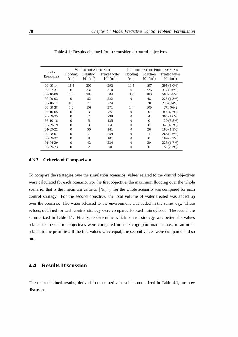
78 Chapter 4 : Model Predictive Control Problem Formulation
Table 4.1: Results obtained for the considered control objectives.
RAIN
EPISODES
WEIGHTED APPROACH LEXICOGRAPHICPROGRAMMING
Flooding Pollution Treated water Flooding Pollution Treated water(cm) 103 (m3) 103 (m3) (cm) 103 (m3) 103 (m3)
99-09-14 11.5 200 292 11.5 197 295 (1.0%)02-07-31 6 236 310 6 226 312 (0.6%)02-10-09 3.6 384 504 3.2 380 508 (0.8%)99-09-03 0 52 222 0 48 225 (1.3%)99-10-17 0.3 71 274 1 70 275 (0.4%)00-09-28 1.2 108 271 1.4 109 271 (0%)98-10-05 0 3 85 0 0 89 (4.5%)98-09-25 0 7 299 0 4 304 (1.6%)98-10-18 0 5 125 0 0 130 (3.8%)00-09-19 0 3 64 0 0 67 (4.5%)01-09-22 0 30 181 0 28 183 (1.1%)02-08-01 0 7 259 0 .4 266 (2.6%)00-09-27 0 8 101 0 0 109 (7.3%)01-04-20 0 42 224 0 39 228 (1.7%)98-09-23 0 2 70 0 0 72 (2.7%)
4.3.3 Criteria of Comparison
To compare the strategies over the simulation scenarios, values related to the control objectives
were calculated for each scenario. For the first objective, the maximum flooding over the whole
scenario, that is the maximum value of‖Ψv‖∞ for the whole scenario was compared for each
control strategy. For the second objective, the total volume of water treated was added up
over the scenario. The water released to the environment wasadded in the same way. These
values, obtained for each control strategy were compared for each rain episode. The results are
summarized in Table 4.1. Finally, to determine which control strategy was better, the values
related to the control objectives were compared in a lexicographic manner, i.e., in an order
related to the priorities. If the first values were equal, thesecond values were compared and so
on.
4.4 Results Discussion
The main obtained results, derived from numerical results summarized in Table 4.1, are now
discussed.

4.4 : Results Discussion 79
1. Important performance improvements were obtained in secondary objectives when lex-
icographic minimization was used. No performance improvements with regard to the
first objective were observed. Maximum flooding remained thesame for the two control
strategies with the exception of two cases (episodes 99-10-17 and 00-09-28). The average
percent increase in treated sewage was 2.3 %. For rain episodes where return rate was
lower than 0.3, the increase was 3.4 %. The percentage increase is shown in parenthesis
in the last column of Table 4.1.
The reasons for the increase in sewage treatment was that thevirtual tanks were used
more efficiently to keep the levels in tanks 7 and 11 higher. This in turn enabled the
inflow into the waste water treatment plants to be higher, as the outflow of these tanks
could be redirected to the treatment plants.
The improvement in sewage treatment lead to an important decrease in pollution released
to the environment. It can be seen in the table that for six rain episodes, sewage released
to the environment was reduced to zero when lexicographic minimization was used. Pol-
lution released (flow and total volume) to the environment isdemonstrated in Figure 4.3
for episode 00-09-27. The reason why no performance improvement was observed for
the first objective was that the same performance could always be achieved by selecting
the weight ratiow1/w3 large enough.
2. In episode 99-10-17, the maximum flooding in the virtual tanks over the whole scenario
was higher when lexicographic minimization was used compared to when the weight
based approach was used. The reason for this is explained in Figure 4.4. The rain episode
has two peaks, a smaller one peaking at time 5 while the largerone at time 43. Looking at
the levels in the tanks it can be seen that the in the lexicographic case, the level is higher
at time 40 when the second peak starts. This causes the flooding to become considerably
larger around time 46. The other scenario where lexicographic minimization performs
worse (episode 00-09-28) has double peaks as well.
The double peak episodes are complicated because poor performance in these cases is
really related to the quality of prediction of rain during the scenarios. The controller
based on lexicographic minimization is operating correctly until the second peak arrives.
It accumulates sewage with the purpose of maximizing sewagetreatment. On the other
hand, when the second peak arrives, this behavior is counterproductive. Notice that if
the objective related to sewage treatment were dropped fromthe objective functions, both
controllers could reduce flooding to zero for episode 99-10-17 and for the other episode,
substantially.

80 Chapter 4 : Model Predictive Control Problem Formulation
0 10 20 30 40 50 60 70 800
1
2
3
4
5
6
0 10 20 30 40 50 60 70 800
1000
2000
3000
4000
5000
6000
7000
time (samples)
Volu
me
tose
a(m3
)F
low
tose
a(m
3/s
)
Figure 4.3: Flow and total volume to environment for episode00-09-27.Solid curve (−), weight based prioritizing, dashed curve (−−)lexicographic prioritizing.
The basic problem is that the two first objectives encourage opposite behaviors in the
controllers. The optimal behavior with regard to the first objective is to have the virtual
tanks as empty as possible to have capacity to be able to receive new peaks of rain. The
second objective strives to store sewage in the system to maximize the sewage treatment.
In the double peak episodes, the lexicographic controller suffers due to its superior ability
to achieve the second objective in the absence of flooding.
If prediction of rain could be improved to the point of being able to recognize multi-
peak episodes, a remedy to the problem described would be to simply drop the secondary
objectives until it is sure that flooding danger is not present.
3. Initially, two cases were considered with regard to the prediction of raind(k) over the
control horizon (30 minutes). In the first case,d(k) was assumed to be equal to the

4.5 : Summary 81
0 10 20 30 40 50 60 70 800
0.5
1
1.5
2
2.5
3
3.5x 10
4
0 10 20 30 40 50 60 70 800
10
20
30
40
50
60
70
LxPmax. capacityWA
Volu
me
(m3)
time (samples)
Rai
n(t
ips/
5min
)
Figure 4.4: Case when lexicographic minimization exhibited poorperformance. The dashed curve is the rain intensity (right axis).
last measurement over the whole horizon. In the other case, the rain was assumed to
be accurately predicted over the horizon. Real rain prediction within an urban area of
the type considered would be somewhere between these two cases, better than assuming
rain constant over the horizon but worse than accurate prediction. The MPC strategy
allows updating the control actions taking into account thereal state of the system and the
precipitation intensity at each sampling time. This state feedback reduces the effect of the
rain prediction error on the control performances. In fact,the difference between the two
cases was found to be small.
4.5 Summary
This chapter presents the lexicographic approach as a solution technique for the multi-objective
optimization that arises in the application of MPC on sewer networks. The possible benefits
of using lexicographic minimization have been demonstrated using a modified version of the
BTC where the most important rain episodes that occurred over an interval of 4 years were

82 Chapter 4 : Model Predictive Control Problem Formulation
studied and the control performance compared with the traditional weight based approach to
express priorities between control objectives. It was shown that performance is similar with
regard to the objective with the highest priority while performance is improved with regard to
objectives of lower priority. For light rain episodes, sewage treatment could be improved 3.5%.
The average improvement for all scenarios was 2.4%.
The numerical value of the performance improvements shouldbe viewed in the context of
the high cost of infrastructures for urban waste water systems. MPC based on lexicographic min-
imization is conceptually very simple and requires a marginal implementation effort compared
to the weight based approach once the model is available. Thefuture increase of complexity
in the sewer networks of big cities, with multiple reservoirs and actuators (gates) will cause
an increment of criteria to take into account in the global optimization function and this imply
an important and difficult off-line effort to find a compromise to tune all the parameters in the
weight-based approach. The lexicographic approach is therefore a very interesting tool for ef-
ficient solution of these kind of problems. The only disadvantage is the increase in the amount
of optimization problems required to obtain the lexicographic minima. However, if a linear
model is used, modern convex optimization routines can easily handle the large scale systems
that occur in the predictive control of urban drainage systems.
Notice that the assumption of a linear system model limits the accuracy in the description
of the real behavior of the sewer network. This motivates to find a different model methodology
that covers all dynamics without loosing the advantages of the MPC for linear systems. Next
chapter deals with this problem and proposes a way to model a sewer network in order to design
a optimization-based controller.
CHAPTER 5
PREDICTIVE CONTROL PROBLEM
FORMULATION BASED ON HYBRID
MODELS
Chapter 4 introduced the application of the predictive control on sewer networks showing im-
portant improvements in the closed-loop system performance and the advantages of this control
strategy over this kind of systems. However, the linear system model considered did not reflect
accurately some particular dynamics and behaviors for someof its components (e.g., weirs, tank
overflows). Therefore, a model methodology that allows to reflect the dynamics of those com-
ponents without leaving the linear framework and without losing all the advantages of the MPC
on the linear system is then needed. This fact has motivated to propose a model methodology
where the nonlinear dynamics of the form (3.8) are taken intoaccount for some of the consid-
ered sewer network elements. These dynamics have been figured out as mode commutations,
where a logic variable determines the continuous behavior of the particular elements and then a
new global behavior of the whole sewer network. Hence, this mixture of continuous dynamics
and logical events define the well known hybrid systems.
This chapter deals with the modeling of a generic sewer network using the hybrid systems
framework. The system is in itself decomposed in functionalsubsystems in order to understand
clearly the “hybridity” related to each component. Using the MLD form, the entire model
is expressed by means of a discrete linear state space representation that is used to design a
MPC law computed by solving a discrete optimization. Both the modeling methodology and
the control design are applied over the BTC, showing the advantages of the proposal and the
83

84 Chapter 5 : MPC Problem Formulation based on Hybrid Model
improvement of the closed-loop system performance respectto the open-loop performance.
5.1 Hybrid Modeling Methodology
The presence of intense precipitation causes some sewers and virtual tanks to surpass their lim-
its. When it happens, the volume above the maximum volume flows to another tank. In this
way, flow paths appear that are not always present and depend of the system state and inputs.
According to this observed behavior in most of the sewer network parts, a model methodology
in order to consider and incorporate overflows and other logical dynamics is needed. Using
hybrid MLD modeling methodology, the global sewer system aswell as each constitutive ele-
ment can be modeled. Here the most common elements are considered. Other elements such
as pumping stations can be easily modeled and added into a sewer network design using the
proposed hybrid modeling methodology. Notice that the hybrid model for the constitutive sewer
network elements discussed in this chapter can be easily modified, keeping their hybrid nature
and becoming new elements.
The hybrid behavior in the considered model of sewer networkis present in the flow links
between tanks, in the tanks themselves (either virtual or real tanks), in the redirection gates and
in the weirs. Network sensors (rain and level gauges) can be also represented as hybrid systems
due to their internal dynamics but they have not been taken into account in this dissertation.
According to this, the network model has been divided into functional parts in order to make
easier the definition of the logical variables and their relation with corresponding flows. These
parts areVirtual Tanks(VT), Real Tanks with Input Gate(RTIG), Flow Links(FL) andRedirec-
tion Gates(RG). In this section, each element is described and its equations within the MLD
framework are expressed. In order to obtain the MLD forms, the following equivalences are
used
[f(x) ≤ 0]←→ [δk = 1] is true iff
f(x) ≤M(1− δk)f(x) ≥ ǫ+ (m− ǫ)δk
(5.1)
and
zk = δkf(x) is true iff
zk ≤Mδk
zk ≥ mδkzk ≤ f(x)−m(1− δk)zk ≥ f(x)−M(1− δk)
(5.2)

5.1 : Hybrid Modeling Methodology 85
T
qin
v
qd
qout
vk
Figure 5.1: Scheme of virtual tank.
whereM,m ∈ R are the upper and lower bounds on the linear functionf(x) for x ∈ X. ǫ > 0
is the computer numeric tolerance, see [BM99a], [TB04].
5.1.1 Virtual Tanks (VT)
This element is modeled as a hybrid system considering the behavior described as follows.
When the maximum volume in virtual tanks is reached, the volume above this maximum amount
is redirected to another tank within the network. This phenomenon can be expressed mathemat-
ically as:
qdk =
(vk−v)∆t if vk ≥ v
0 otherwise(5.3a)
qoutk =
βv if vk ≥ vβvk otherwise
(5.3b)
wherevk corresponds to the tank volume (system state) andv is its maximum volume capacity.
Flow qdk is the overflow from the tank, see Figure 5.1. For a feasible solution of the control
problem, the virtual tank volume can not be limited with hardconstraints.
Hence, in order to obtain the MLD model, the condition of overflow existence is considered

86 Chapter 5 : MPC Problem Formulation based on Hybrid Model
defining the logical variable
[δk = 1]←→ [vk ≥ v], (5.4)
which implies that flowsqdk andqoutk are defined through this logical variable as:
z1k = qdk
= δk
[(vk − v)
∆t
](5.5a)
z2k = qoutk
= δkβv + (1− δk)βvk. (5.5b)
The corresponding difference equation for the tank in function of the auxiliary variables is writ-
ten as:
vk+1 = vk + ∆t[qink − z1k − z2k], (5.6)
whereqink is the tank inflow,z1k is related to the tank overflow andz2k is related to the tank
output. Notice thatqink collects all inflows to the tank, which could be outflows from tanks
located at a more elevated position within the network, linkflows, overflows from other tanks
and/or sewers and rain inflows.
Hence, the MLD expression (2.8) for this element, taking thetank volume as the system
output, would be written as follows:
vk+1 = vk + [∆t] qink +[− ∆t −∆t
] [ z1k
z2k
]
yk = vk
−Mv + v
v
(Mv − v)/∆t
v/∆t
−v/∆t
−(Mv − v)/∆t
βv
β(Mv − v)
−β(Mv − v)
βv
0
0
δk +
0 0
0 0
−1 0
1 0
−1 0
1 0
0 −1
0 1
0 −1
0 1
0 0
0 0
[z1k
z2k
]≤
−1
1
−1/∆t
1/∆t
0
0
0
0
−β
β
1
−1
vk +
v
0
Mv/∆t
0
0
0
0
βMv
0
0
0
Mv
(5.7)
whereMv is related to the maximum value of the state variable which inthe case of virtual tanks

5.1 : Hybrid Modeling Methodology 87
qin
qa
qb
qout
v
vkT
Figure 5.2: Scheme of a real tank with input gate.
would be unbounded, i.e.,Mv →∞.
5.1.2 Real Tanks with Input Gate (RTIG)
As was said before, the real tanks are elements designed to retain water in case of severe weather.
For this reason, both the tank inflow and outflow could be controlled. On the other hand, the tank
inflow is constrained by the actual volume present in the realtank, by its maximum capacity and
by the tank outflow. Since this category of tanks are considered without overflow capabilities,
the inflow is pre-manipulated using a redirection gate, reason that causes the consideration of
this component within the modeling of this element. Figure 5.2 shows a scheme of this element.
When the model for open-loop is considered (no manipulated links), the flow throughqa
due to its maximum capacity is defined by
qa1k =
qa if qin ≥ qa
qink otherwise(5.8)
whereqink is the inflow to the element andqa represents the maximum flow through sewerqa.

88 Chapter 5 : MPC Problem Formulation based on Hybrid Model
However, if the inflowqa1k causes the real tank to overflow, such inflow have to be reducedto a
flow equivalent to the volume that fills the tank. That is:
qa2k =
vrk if qa1k − qoutk ≥ vrk
qa1k otherwise(5.9)
wherevrk =(
(v−vk)∆t + qoutk
)andqoutk denotes the tank outflow. The MLD form under the
initial assumptions is obtained as follows. Defining
[δ1k = 1]←→ [qink ≥ qa], (5.10)
it is possible to obtain an auxiliary continuous variable
z1k = qak
= δ1k qa + (1− δ1k) qink. (5.11)
For qa2k, the following logical variable is defined as:
[δ2k = 1]←→[z1k − qoutk ≥
(v − vk)
∆t
](5.12)
and hence the auxiliary variable equivalent to the new real tank inflow is expressed as:
z2k = qa2k
= δ2k
[(v − vk)
∆t+ qoutk
]+ (1− δ2k) z1k. (5.13)
Finally, according to the mass conservation in the includedinput gate,qbk is defined as
qbk = qink − z2k and the corresponding difference equation for the tank in function of the
auxiliary variables is:
vk+1 = (1− β∆t)vk + ∆tz2k (5.14)
The MLD expression (2.8) taking the tank volume as the systemoutput is written as:
vk+1 = [1− β∆t] vk +[
0 ∆t] [ z1k
z2k
]
yk = vk
(5.15)

5.1 : Hybrid Modeling Methodology 89
and the Inequality (2.8c) collecting 12 linear inequalities with:
E1 =[
1 −1 0 0 −1 1 0 0 0 0 0 0]T
E21 =
[−qa (qin − qa) 0 0 (qin − qa) qa
0 0 − v∆t
(qin − βv) 0 0
]
E22 =
[−qa −(qin − qa) 0 0 0 0
0 0 − v∆t
(qin − βv) 0 0
]
E2 =[E21 E22
]T
E3 =
[0 0 −1 1 −1 1 −1 1 1 −1 0 0
0 0 0 0 0 0 0 0 −1 1 −1 1
]T
E4 =[
0 0 1∆t− β −
(1
∆t− β
)0 0 0 0 0 0 1
∆t− β −
(1
∆t− β
) ]T
E51 =[−qa qin − v
∆t
(v(
1∆t− β
)+ qin
)(qin − qa) qa
]
E52 =[−qa qa (qin − βv) v
∆t− v
∆tv∆t
]
E5 =[E51 E51
]T
(5.16)
According to the use of this element regarding either the simulation or the prediction model,
both the tank inflow and output could be manipulated. Hence, two possibilities are considered
and outlined below.
1. The RTIG element is used to build a global hybrid model for simulation within a con-
trol loop. In this case, both flowsqak and qoutk have to fulfill the respective physical
constraints
qa≤ qak ≤ qa (5.17)
qout≤ qoutk ≤ qout (5.18)
whereqa
andqout
are the minimum flows through sewersqa andqout, respectively. The
values of these minimum flows are supposed to be zero in nominal configuration (no
faults). For this case, the MLD model of the element includesthe constraints (5.17)-
(5.18) and validates the possible inputs out of the range.
The expressions of the dynamics in MLD form according to thisassumption are obtained
as follows. The given input valueq⋆a have to be smaller than the inflow to the element.
Otherwise,q⋆a does not have sense because the differenceq⋆
a − qink corresponds to a

90 Chapter 5 : MPC Problem Formulation based on Hybrid Model
nonexistent water entering to the element. This idea is expressed mathematically as:
qa1k =
q⋆a if q⋆
a ≥ qink
qink otherwise.(5.19)
Now, the upper bound of the link flow adds another condition for q⋆a, given by the upper
physical bound as:
qa2k =
qa1k if qa1k ≤ qa
qa otherwise.(5.20)
Finally, the maximum tank capacity also constrains the value of q⋆a to:
qa3k =
vr if qa2k − qoutk ≥ vr
qa2k otherwise.(5.21)
Moreover, the given valueq⋆out is also restricted by its physical constraint in (5.18). The
corresponding expression that restricts this flow due to theupper physical bound is:
qout1k =
q⋆out if q⋆
out ≤ qout
qout otherwise(5.22)
and then the expression that restricts this flow due to the actual tank volume is written as:
qout2k =
qout1k if qout1k ≥ βvk
βvk otherwise.(5.23)
Again, the flowqbk is defined by mass conservation condition in the input gate as:
qbk = qink − qa3k. (5.24)
The MLD model for this case is then obtained from the expressions presented in Table
5.1, which define the correspondingδ andz variables. For this case,qbk = qink − z5k.
The difference equation related to the tank is:
vk+1 = vk + ∆t (z5k − z4k) . (5.25)
Finally, the MLD expression (2.8) taking the volume as the system output can be written

5.1 : Hybrid Modeling Methodology 91
Table 5.1: Expressions forδ andz variables in RTIG element consideringmanipulated links in closed-loop simulation.
Logical variableδ Auxiliary variablez
[δ1k = 1]←→ [q⋆a ≥ qink] z1k = δ1kq
⋆a + (1− δ1k)qink
[δ2k = 1]←→ [z1k ≤ qa] z2k = δ2kz1k + (1− δ2k)qa
[δ3k = 1]←→ [q⋆out ≤ qout] z3k = δ3kq
⋆out + (1− δ3k)qout
[δ4k = 1]←→ [z3k ≥ βvk] z4k = δ4kz3k + (1− δ4k)βvk
[δ5k = 1]←→ [z2k − z4k ≥ vrk] z5k = δ5kvrk + (1− δ5k)z2k
as:
vk+1 = vk +[
0 0 0 −∆t ∆t]
z1k
z2k
z3k
z4k
z5k
yk = vk
(5.26)
and the inequality (2.8c) collecting 30 linear inequalities, which is automatically gener-
ated by HYSDEL.
2. The RTIG element is used to build a global hybrid model for prediction within a control
loop. In this case, constraints (5.17) and (5.18) are included in the control law design so
they are not taken into account when the MLD model of the element is done. Thus, the
expressions of the element dynamics can be obtained as follows. In order to restrict the
value of the given inputq⋆a in order to fulfill the mass conservation condition in the input
gate, the flow through linkqa is expressed as:
qa1k =
q⋆a if q⋆
a ≤ qink
qink otherwise(5.27)
However, the tank capacity also restricts the tank inflow according to the expression:
qak =
qa1k if qa1k − qoutk ≤ v−vk
∆t
v−vk
∆t otherwise(5.28)

92 Chapter 5 : MPC Problem Formulation based on Hybrid Model
Table 5.2: Expressions forδ andz variables in RTIG element consideringmanipulated links in closed-loop prediction.
Logical variableδ Auxiliary variablez
[δ1k = 1]←→ [q⋆a ≤ qink] z1k = δ1kq
⋆a + (1− δ1k)qink
[δ2k = 1]←→[z1k − z3k ≤ v−vk
∆t
]z2k = δ2kqa1k + (1− δ2k)
v−vk
∆t
[δ3k = 1]←→ [q⋆out ≤ βvk] z3k = δ3kq
⋆out + (1− δ3k)βvk
About the tank outflow, the given inputq⋆out is restricted according to the outflow related
to the actual volume. That is:
qoutk =
q⋆out if q⋆
out ≤ βvk
βvk otherwise(5.29)
The expressions forδ andz variables in order to obtain the corresponding MLD model
are collected in Table 5.2.
The MLD expression (2.8) for this element in this case, taking the tank volume as the
system output, is written as follows:
vk+1 = vk +[
0 −∆t ∆t]
z1k
z2k
z3k
yk = vk
(5.30)
and the inequality (2.8c) collecting 18 linear inequalities, which is automatically gener-
ated by HYSDEL.
Notice that a MLD model with fewer logical variables can be used for instance in the design
of a model predictive controller, what reduces the complexity and the computation time of the
control problem solution.
5.1.3 Redirection Gates (RG)
These type of elements within a sewer network are used to redirect flow at a certain point in
the network. Assuming thatqak is manipulated, outflowqbk in Figure 5.3 has to fulfill the mass

5.1 : Hybrid Modeling Methodology 93
qin
qa
qb
Figure 5.3: Scheme of redirection gate element.
conservation law in this point. Generally,qak is assumed to be limited, in which caseqbk is
unlimited. The reason for this assumption is that if both outflows are limited, the situation could
occur thatqink would be larger than the sum of these limits, causing the total network to have
no feasible solution. The expressions that describe the element dynamics are:
qak =
qink if qink ≤ qa
qa otherwise(5.31a)
qbk = qink − qak. (5.31b)
If the flow through sewerqa is imposed (for instance computed by means of a control law),its
new expression is now written as:
qak =
qa if q⋆
a > qa
q⋆a otherwise
(5.32)
whereq⋆a corresponds to the imposed/computed value for the flowqak, while qbk follows the
expression (5.31b).
This element may have a kind of MLD model depending ifqa is considered as a manipulated
link or not. In any case, this is an static element, i.e., there is not any state variable in the MLD
model. This element only adds moreδ andz variables to the global MLD model of the sewer
network.

94 Chapter 5 : MPC Problem Formulation based on Hybrid Model
1. qa as free link:Basically this model is used for open-loop simulation. The hybrid dynam-
ics are defined by the maximum flow through sewerqa, what causes the definition of the
auxiliary logic variable
[δk = 1]←→ [qink ≥ qa] (5.33)
and redefine the flowqak as:
zk = qak
= δk qak + (1− δk) qink (5.34)
Thus, the flow through sewerqb is immediately defined by the mass conservation as:
qbk = qink − zk (5.35)
In this case, 6 linear inequalities are defined as in (2.8c) as:
−qa
qin − qa
qin − qa
qa
−qa
−qin + qa
δk +
0
0
−1
1
−1
1
zk ≤
1
−1
−1
1
0
0
qink +
qa
qin
qin − qa
qa
−qa
qa
(5.36)
Notice that sewerqa is considered as the main path for the flow.
2. qa as manipulated link:In this case, a closed-loop is considered so the element could be
used within either a simulation or a prediction model. In thefirst case (simulation model),
the hybrid dynamics are defined taking into account the system constraintqa≤ qa ≤ qa.
This constraint is supposed to be added to the global model when the control law is de-
signed. Thus, a couple ofδ andz variables are defined in order to validate that the given
value ofqa fulfills to the mentioned constraint. The definitions of these δ variables de-
pending on the hybrid condition are explained as follows. For the condition of water
sufficiency, the logical variableδ1 is determined as:
[δ1k = 1]←→ [qak ≥ qink] (5.37)
and for the condition related to the upper limit of sewerqa the logical variableδ2 is

5.1 : Hybrid Modeling Methodology 95
determined as:
[δ2k = 1]←→ [qak ≤ qa] . (5.38)
Then, the corresponding auxiliary continuous variables are:
z1k = δ1kqak + (1− δ1k)qink (5.39a)
z2k = δ2kz1k + (1− δ2k)qak. (5.39b)
Again, the flow through sewerqb is immediately defined by the mass conservation as:
qbk = qink − z2k. (5.40)
Here, 12 linear inequalities are defined according to Inequality (2.8c) with:
E1 =
[0 0 0 0 −1 1 −1 1 1 −1 0 0
0 0 0 0 0 0 0 0 −1 1 −1 1
]T
E21 =
[−qa qin 0 0 qa −qin
0 0 −qa 0 0 0
]
E22 =
[−qin qa 0 0 0 0
0 0 (qin − qa) qa −qa −(qin − qa)
]
E2 =[E21 E22
]T
E3 =
[0 0 0 0 −1 1 −1 1 1 −1 0 0
0 0 0 0 0 0 0 0 −1 1 −1 1
]T
E5 =[
0 qin −qa qa qa qin 0 0 (qin − qa) qa −qa qa
]T
(5.41)
On the other hand, when a prediction model is considered,qa theoretically fulfills the
design constraintqa≤ qa ≤ qa, but the values ofq
aand qa are information data of
the control algorithm, so they could be different from the physical bounds (this could be
caused, for instance, by a fault effect). Hence, the definitions
[δk = 1]←→ [qak ≥ qink] (5.42)
and
zk = δ1kqak + (1− δ1k)qink (5.43)
are given in order to fulfill the mass conservation condition. Then, the element adds to

96 Chapter 5 : MPC Problem Formulation based on Hybrid Model
the global model the following set of 6 inequalities according to Inequality (2.8c):
−qa
qin
qa
qin
−qin
−qa
δk +
0
0
−1
1
−1
1
zk ≤
1 −1
−1 1
0 −1
0 1
−1 0
1 0
[qink
qak
]+
0
qin
qa
qin
0
0
(5.44)
In conclusion, the selection of whatever of these two modelsis directly related to the use of
the RG element within the global model and the use of the global model in itself.
5.1.4 Flow Links (FL)
Flow links between tanks have limited capacity. As the flow from virtual tanks can not be
controlled, when this limit is exceeded, the resulting overflow might be redirected to a tank to
which the original link was not connected. When RG are used toredirect the virtual tank outflow,
the unmanipulated link associated to the RG could surpass the maximum sewer capacity. Hence,
the sewer overflow is sent to a tank located in a lower level of the sewer network or flows to
the environment as water losses. The behavior explained canbe represented with the following
equations (see Figure 5.4):
qbk =
qb if qin > qb
qink otherwise(5.45a)
qck =
qink − qb if qin > qb
0 otherwise(5.45b)
whereqb is the maximum flow throughqb, qink is the element inflow andqck corresponds to the
outflow.
For the MLD model of this element, only one logical variable is needed. It is defined from
the hybrid overflow condition as:
[δk = 1]←→ [qin ≥ qb] (5.46)

5.1 : Hybrid Modeling Methodology 97
qin
qb
qc
Figure 5.4: Scheme for flow links.
and the auxiliary continuous variables that define the flowsqbk andqck are respectively:
z1k = qbk
= δk qb + (1− δk) qink (5.47a)
z2k = qck
= δk (qink − qb). (5.47b)
Notice that, as in the case of the element presented before, this is also a static element, so it
only adds moreδ andz variables to a global MLD model of the sewer network as well asmore
constraints in the corresponding Inequality (2.8c) as follows:
−qin + qb
qb
qb
qin − qb
−qin + qb
−qb
qin − qb
qb
−qb
−qin + qb
δk +
0 0
0 0
−1 0
1 0
−1 0
1 0
0 −1
0 1
0 −1
0 1
zk ≤
−1
1
0
0
−1
1
−1
1
0
0
qink +
qb
0
0
qin
0
0
qin
0
0
0
(5.48)

98 Chapter 5 : MPC Problem Formulation based on Hybrid Model
whereqin corresponds to the maximum inflow to the element.
Both overflow in VT and overflow in FL do not necessarily go to the immediately next ele-
ment in the network. Generally, FL overflows do not only go to VT but also to the environment.
In these cases, these flows represent losses to the environment (flows to the sea or rivers without
previous treatment).
5.1.5 The Whole MLD Catchment Model
The total sewer network is constructed by connecting the network inflows (rain) and outflows
(sewer treatment plants or pollution) with the inflows and outflows of the tanks as well as con-
necting the tanks themselves. Notice that it is possible to obtain the global MLD model by
connecting all elements in order to build the equivalent model scheme as shown in Figure 5.5
for the BTC. However, a software tool that allows to interpret the corresponding inputs and out-
puts of each element in its MLD form and translates them into aglobal MLD is now pending of
implementation. The final tool would have the advantages of atool for sewer networks known
as CORAL [FCP+02], but including the hybrid model framework into its kernel, what allows
to improve the computation of optimal control laws since theconsidered lineal model of the
system despite of the global dimension of the network.
The manipulated variables of the system, denoted asqu, are the manipulated variables of
each component as described before. The whole sewer networkexpressed in MLD form can be
written as:
vk+1 = Avk +B1quk +B2δk +B3zk +B4dk (5.49a)
yk = Cvk +D1quk +D2δk +D3zk +D4dk (5.49b)
E2δk + E3zk ≤ E1quk + E4vk + E5 + E6dk (5.49c)
wherev ∈ V ⊆ Rnc+ corresponds to the vector of tank volumes (states),qu ∈ U ⊆ R
mic+ is
the vector of manipulated sewer flows (inputs),d ∈ Rmd+ is the vector of rain measurements
(disturbance), logic vectorδ ∈ 0, 1rℓ collects the Boolean overflow conditions and vectorz ∈R
rc+ is associated with variables that appear depending on system states and inputs. Variables
δ andz are auxiliary variables associated with the MLD form. Equation (5.49c) collects the
set of system constraints as well as translations from logicpropositions. Notice that this model
is a more general MLD than was presented in [BM99a] due to the addition of the measured
disturbances.

5.1 : Hybrid Modeling Methodology 99
VT1 VT2 RTIG
VT4
VT5
VT6
VT7
VT8
VT9
VT10
VT11
VT12
FL14
FL24
FL96
FLc210 FL945 FL12s
FLR1FLR2
FLR3
FLR4
FLR5
d1
d2
d4
d5
d6
d7
d8
d9
d10
RG1
RG1
Σ
Σ
Σ
Σ
Σ
Σ
Σ
Σ
Σ
fsea
fsea
fsea
fsea
fsea
fsea fsea
fsea
fsea fsea
fenv
WWTP 1 WWTP 2
K
Figure 5.5: BTC scheme using hybrid network elements.
Likewise, measured disturbances may be considered even as inputs or system states. Ac-
cording to the case,qu andd could be collected in a single vector of system inputs depending
on the control law algorithm used. Hence, the MLD form could be rewritten as:
vk+1 = Avk + B quk +[B2 B3
] [ δk
zk
](5.50a)
yk = Cvk + D quk +[D2 D3
] [ δk
zk
](5.50b)
[E2 E3
] [ δk
zk
]≤ E quk +
[E4 E5
] [ vk
1
](5.50c)

100 Chapter 5 : MPC Problem Formulation based on Hybrid Model
where vector quk collects the control inputs and measured disturbances. Moreover,
B = [B1 B4], D = [D1 D4] andE = [E1 E6].
On the other hand, assuming that the rain prediction overHp obeys to a preestablished linear
dynamic described asdk+1 = Addk, the MDL (5.49) form could be rewritten in this case as:
[vk+1
dk+1
]=
[A B4
0 Ad
][vk
dk
]+
[B1 B2 B3
0 0 0
]
quk
δk
zk
(5.51a)
yk =[C 0
] [ vk
dk
]+[D1 D2 D3
]
quk
δk
zk
(5.51b)
[E2 E3
] [ δk
zk
]≤
[E4 E6
] [ vk
dk
]+[E1 E5
] [ quk
1
](5.51c)
In general, this assumption is an open research topic. Different types of rain prediction can
be considered since this procedure can be development in a either theoretical way (statistical,
AR models, etc) [SA00] or practical way (radars, meteorological satellites, etc) [YTJC99]. Ac-
cording to [CQ99], different assumptions can be done for therain prediction when an optimal
control law is used in the RTC of sewer networks. Results showthat the assumption of con-
stant rain over a short prediction horizon gives results that can be compared with the assumption
of known rain over the considered horizon, confirming similar results reported in [GR94] and
[OMPQI05]. According to this, matrixAd can be set as a identity matrix of suitable dimensions.
5.2 Predictive Control Strategy
This section presents the detailed description of the control strategy applied on sewer networks
considering an hybrid system model. The different aspects discussed here are presented for the
particular case study of this thesis but can be easily extrapolated to other sewage system topolo-
gies. The concepts and definitions of Section 2.2 are appliedin this section in a straightforward
manner but taking into account the particular notation usedfor sewer networks. Hence, the
sequences for manipulated flow and volumes are defined as:
vk = v1|k, v2|k, . . . , vHp|kquk = qu0|k, qu1|k, . . . , quHp−1|k
(5.52)

5.2 : Predictive Control Strategy 101
and the expression for the admissible input sequence respect to the initial volumev0|k , vk ∈ V
is now written as:
QU (vk) , quk ∈ UHp |vk ∈ V
Hp. (5.53)
5.2.1 Control Objectives
In the design process of the MPC controller based on a hybrid model of the system, the control
objectives are the same as in the controller design done in Chapter 4 (Section 4.2.1). According
to the hybrid model for sewer networks proposed in Section 5.1, all overflows and flows to
treatment plants are defined by auxiliary variablesz. However, they can be also defined as
system outputs, these being either individual (over)flows or sums of (over)flows according to
the case.
5.2.2 The Cost Function
Each control objective defines or can define one term in the cost function. Hence, the expression
of that function depends on its constitutive variables (auxiliary or output type). In general form,
the structure for the cost function in (2.14a) has the form:
J(quk,∆k, zk, vk) ,
Hp−1∑
i=0
∥∥Qz(zk+i|k − zr)∥∥
p+
Hp−1∑
i=0
∥∥Qy(yk+i|k − yr)∥∥
p(5.54)
whereQz andQy correspond to weight matrices of suitable dimensions fulfilling the conditions
in (2.15) andzr, yr are reference trajectories related to auxiliary and outputvariables, respec-
tively. For the objectives 1 and 2, the references are zero flow. For the third objective, the
references are the maximum capacity of the associated sewage treatment plants. Priorities are
set by selecting matricesQz andQy. The normp can be selected asp = 1, 2 or p =∞. Notice
that since all performance variables are positive, the casewhenp = 1 is actually a simple sum
of the performance variables.
According to the definition of the control objectives done inSection 5.1 and in the case of
having the complementary fifth objective, notice that the cost function adopts the form:
J(quk,∆k, zk, vk) , ‖Qvfvrt(Hp|k)‖p +
Hp−1∑
i=0
∥∥Q(zk+i|k − zr)∥∥
p(5.55)

102 Chapter 5 : MPC Problem Formulation based on Hybrid Model
whereQvfis the corresponding weight matrix of suitable dimensions.
5.2.3 Problem Constraints
The modeling approach is based on mass conservation. Due to this, physical restrictions have
to be included as constraints in the optimization problem. The sum of inflows into nodes that
connect links have to be equal the outflow. The control variables are limited to a range given in
(3.7). The constraints associated to the MIPC problem are ingeneral the constraints associated
with the hybrid behavior as well as the system physical constraints for manipulated links and
real tanks and the initial condition corresponding to the measurements of the tanks volumes at
time instantk ∈ Z+.
All the constraints can be expressed on the form given by (5.49c). The physical constraints
are considered ashard constraintsinto the control problem. On the other hand, the overflows in
sewers and virtual tanks are considered assoft constraintsand a constraint manager could be de-
signed and implemented to solve the control problem with constraints prioritization [KBM+00].
5.2.4 MIPC Problem
According to the aspects described before, the predictive control problem for a sewer network
considering its hybrid model is defined as the OOP
minquk∈ QU (vk),∆k,zk
J (quk,∆k, zk, vk) (5.56a)
subject to
vk+i+1|k = Avk+i|k +B1 quk+i|k +B2 δk+i|k +B3 zk+i|k +B4 dk+i|k
yk+i|k = C vk+i|k +D1 quk+i|k +D2 δk+i|k +D3 zk+i|k +D4 dk+i|k
E2 δk+i|k + E3 zk+i|k ≤ E1 quk+i|k + E4 vk+i|k +E5 + E6 dk+i|k
dk+i+1|k = Ad dk+i|k
(5.56b)
for i = 0, . . . ,Hp − 1. Assuming that the problem is feasible forv ∈ V, i.e.,QU (v) 6= ∅, the
receding horizon philosophy is then used considering as theMPC law
quMPC(vk) , qu∗0|k (5.57)
and the entire optimization process is repeated for timek + 1.

5.3 : Simulation and Results 103
5.3 Simulation and Results
5.3.1 Preliminaries
The purpose of this section is to show the performance of HMPCfor realistic episodes of rain
storms. The assumptions made for the implementation will bepresented and their validity dis-
cussed before the results are given.
The transformation of the hybrid system equations into the MLD form requires the appli-
cation of the set of given rules in (5.1) and (5.2). The higherlevel language and associated
compiler HYSDEL is used here to avoid the tedious procedure of deriving the MLD form by
hand. Given the MLD model, the controllers were designed andthe scenarios simulated using
the HYBRID TOOLBOX for MATLAB r (see [Bem06]). Moreover, ILOG CPLEX 9.1 has been
used for solving MIP problems.
The considered system is shown in Figure 5.6. The dashed lines represent the overflow
from tanks and sewers. These lines therefore represent the hybrid behavior of the network. The
catchment hybrid model has 12 state variables corresponding to the volumes in the tanks (11
virtual and 1 real), 4 control signals related to the manipulated flows in gates (3 redirection
gates and 1 retention gate) and 11 perturbation signals related to the inflow rain of each virtual
tank.
The nominal operating ranges of the control signals, the description of the variables in Figure
5.6 and all needed parameters are given in Tables 3.1 and 3.2.Table B in Appendix B collects the
auxiliary variablesz defined for the BTC and relate them with the control objectives discussed
in Section 4.2.1. In order to define the outputs in the global MLD of the network, the following
outputs are defined:
y1 =∑
i
zstrv , y2 =∑
i
zstrq , y3 = z41 and y4 = z43.
5.3.2 MLD Model Descriptions and Controller Set-up
Two different MLD models can be needed to simulate the scenarios, one for the HMPC con-
troller, MLDC , and one to simulate the plant, MLDP . Notice that physical constraints are
included into the model MLDC and the solution to the optimization problem respects these
constraints in the nominal case when there is no mismatch between the model and the plant.

104 Chapter 5 : MPC Problem Formulation based on Hybrid Model
T1
T2
T3
T4
T5
T6
T7
T8
T9
T10
T11
T12
w1
w2
w4
w5
w6
w7
w8
w9
w10
w11
w12
qu1
qu2
qu3
qu4
R1
R2
R3
R4
R5
q14
q24
q96
q910
qc210
q945
q946
q10M
q57
q68
q7M
q128
q12s
q811
q8M
q11B
q11M
q7L
C1
C4
C2
C3
P13
P14
P16
P16
P16
P19
P20
P20P20
P20
P20
L39
L41
L80
L16
L53
L9
L27
L
L
L3
L11
L47
L56
L7
L8
MEDITERRANEAN
SEA
Escola
Industrial
tank
Weir overflowdevice
Real tank
Virtualtank
rainfall
Level gaugeRedirection
gate
Retention gate
(WWTP 1)LlobregatTreatment
Plant
(WWTP 2)Besos
TreatmentPlant
Figure 5.6: BTC diagram for hybrid design.

5.3 : Simulation and Results 105
Otherwise, the solution to the optimization problem might not respect the physical restrictions
of the network. The model MLDP is therefore augmented so that the control signals from
the controller are adjusted to respect the physical restrictions of the whole network. MLDP
contained more auxiliary variables for this reason.
Another alternative consists in using the set of equations given by the virtual tank modeling
of the network as the plant, which implies that the MLDP is not needed. For the simulations
and results presented next, this second alternative is used. The MLDC model implemented has
22 logical variables and 44 auxiliary variables, which implies that for each time instantk ∈ Z+
and considering the prediction horizonHp = 6, 222×6 = 5.4×1039 LP problems (forp = 1,∞)
or QP problems (forp = 2) could be solved in the worst case.
In this case of control design where a hybrid model of the system is taken into account,
tuning techniques based on weighted approach are implemented. Tuning proposes such as the
lexicographic approach presented in Chapter 4 for linear MPC is not suggested to be applied in
predictive control of hybrid systems because the complexity of the optimization problem when
the system is considered of large scale. Notice that if the lexicographic approach is implemented,
for each time instantk over the scenario, a number of discrete optimization problems equals to
the number of control objectives have to be solved. This factcan cause high computation costs
and important complexity in the solution algorithms. Chapter 6 deals with these problems and
proposes some possible solutions.
Hence, for this case where the tuning by weighted approach isdone, the weight matrices
used for the cost function (5.54) are given by
Qy =
diag(wstrvIn wstrqIn wWWTPIn) if only y are used inJ
wWWTPIn if z andy are used inJ(5.58a)
and
Qz =
diag(wstrvIn wstrqIn) if z andy are used inJ
0 otherwise(5.58b)
where the description of the weight parameterswi are collected in Table 5.3 andIn corresponds
to a identity matrix of suitable dimensions. Moreover, the vector of referenceszr is always zero

106 Chapter 5 : MPC Problem Formulation based on Hybrid Model
Table 5.3: Description of parameters related to weight matrices in HMPC.
Parameter Description
wstrv Weight for the flow to the street due to tankswstrq Weight for the flow to the street due to linkwWWTP Weight for the flow to treatment plants
andyr is set as:
yr =
[On On On 1n q7L 1n q11B]T if only y are used inJ
[On 1n q7L 1n q11B]T if z andy are used inJ(5.59)
whereOn is a vector of zeros and1n is a vector of ones, both with suitable dimensions for each
set of variables related to each control objective.
As was said before, the prediction horizonHp is set as 6, what is equivalent to 30 minutes
(with the sampling time∆t = 300 s). The optimal solutions are computed for a bounded
time intervalk ∈ [0, 100], which implies around 8 hours. The computational times refer to a
MATLAB r implementation running on a INTELr PENTIUMr M 1.73 GHz machine.
5.3.3 Performance Improvement
The performance of the control scheme is compared with the simulation of the sewer network
without control when the manipulated links have been used aspassive elements, i.e., the amount
of flows qu1k, qu2k andqu4k only depend on the inflow to the corresponding gate and they are
not manipulated (see Section 5.1) whilequ3k is the natural outflow of the real tank given by
(3.3). The control tuning is done taking into account the prioritization of the control objectives.
In a preliminary study, different norms, cost function structures and cost function weights
wi have been used. In order to give a hierarchical priority to the control objectives, the relation
of wi between objectives is an order of magnitude. Table 5.4 summarizes the obtained results
for a heavy rain episode occurred on September 14, 1999 (see Figure 3.8(a)).
The use of infinity norm for the first and second objectives implies the minimization of the
greatest flow to the street caused by one of the 11 virtual tanks and/or the 6 considered sewers.

5.4 : Summary 107
Table 5.4: Obtained results of closed-loop performance using rain episodeoccurred on September 14, 1999.
NormVariables Tuning Flooding Pollution Treated W.
in J wstrv ×103 (m3) ×103 (m3) ×103 (m3)
∞ only y 10 84.1 225.3 279.4∞ only y 0.1 84.2 225.3 279.4∞ y andz 100 100.9 225.9 278.7∞ y andz 0.1 103.2 225.6 279.12 y andz 1 94.3 228.3 276.12 only y 0.01 92.8 223.5 280.8
However, in the case of two or more virtual tanks or sewers have overflow, only the worst case
will be minimized.
Taking into account that the system performance in open-loop for the considered rain
episode has a flooding volume around108000, a pollution volume of225900 and a volume
treated water of278300 (all in m3), the improvement reached is between 4.5% and 22.1% for
the first objective and the other objectives keep almost in the same values for most of the cases,
fulfilling the desired prioritization principle implemented making the control tuning by weighted
approach. However, it was observed that some simulations did not run with some combination
of selected parameters because numerical problems or the parameters setting made that no im-
provement was reached in the system performance.
Table 5.5 summarizes the results for ten of the more representative rain episodes in
Barcelona between 1998 and 2002. The results were obtained consideringp = 2 and a cost func-
tion containing only output variables withwstrv = 10−2. The system performance in general is
improved when the hybrid model based predictive control strategy is applied (see percentages
for some values).
5.4 Summary
The possibility of having a linear model of a sewer network taking into account the logical
dynamics given by some constitutive elements is discussed in this chapter. A new modeling
methodology for sewer networks using a MLD form is proposed and widely explained. This fact
makes possible to take advantage of the MPC capabilities in order to design a control strategy

108 Chapter 5 : MPC Problem Formulation based on Hybrid Model
Table 5.5: Obtained results of closed-loop performance using tenrepresentative rain episodes.
RainEpisodes
Open-Loop Closed-LoopFlooding Pollution Treated W. Flooding Pollution Treated W.×103 (m3) ×103 (m3) ×103 (m3) ×103 (m3) ×103 (m3) ×103 (m3)
99-09-14 108 225.8 278.4 92.9(14%) 223.5 280.702-10-09 116.1 409.8 533.8 97.1(16%) 398.8 544.999-09-03 1 42.3 234.3 0(100%) 44.3 232.302-07-31 160.3 378 324.4 139.7(13%) 374.6 327.899-10-17 0 65.1 288.4 0 58.1(11%) 295.300-09-28 1 104.5 285.3 1 98(6%) 291.998-09-25 0 4.8 399.3 0 4.8 398.801-09-22 0 25.5 192.3 0 25 192.402-08-01 0 1.2 285.8 0 1.2 285.801-04-20 0 35.4 239.5 0 32.3(9%) 242.5
for the entire system.
The control design is then proposed and the discrete optimization problem is described
and discussed. Both the main improvements of the technique and the possible problems of
implementation are pointed out. The modeling methodology as well as the controller design are
implemented in simulation over the BTC and the main obtainedresults are presented and also
discussed.
The main issue of this chapter lies on the real implementation of the proposed control design.
Some of the simulations presented in Tables 5.4 and 5.5 need high computation times, which
implies that the use on-line of the controller could not be possible in some cases. This fact
makes that the idea of having a predictive controller when the system model is hybrid and has
an important size should be thought only for off-line proposes. In this sense, Chapter 6 deals
with the time computation problem, proposing and discussing some ways of solution.

CHAPTER 6
SUBOPTIMAL HYBRID MODEL
PREDICTIVE CONTROL
6.1 Motivation
The results obtained in the simulation study of the previouschapter show that important perfor-
mance improvements can be accomplished when HMPC is appliedto sewer networks. Further-
more, the hybrid modeling methodology is very rich and allows the straightforward treatment
of hybrid phenomena such as overflow and flooding. HMPC has been applied successfully to
a variety of control problems the last years using several approaches, see [BBM98], [Sch99],
[TLS00], [LR01], [BBM02], among others.
However, the underlying optimization problem of HMPC is combinatorial andNP-hard
[Pap94]. The worst-case computation time is exponential inthe sense of the amount of combi-
natorial variables. In Figure 6.1 it is shown how this problem manifests itself for the application
under investigation in this thesis.
In the top graph, rain intensity is shown related to the five rain gauges in the BTC for the
critical portion (second rain peak) of the rain episode occurred on October 17, 1999. This
episode was relatively intensive with a return rate of 0.7 years within the city of Barcelona.
In the second graph, the computation time to solve the MIP is shown as a function of sample
for the same scenario. Recalling that the desired sampling time for this system is 300 seconds,
it can be seen that the MIP solver is incapable of finding the optimum within the desired sam-
pling time. Furthermore, it is seen that computation time varies greatly. Before sample 16 the
109

110 Chapter 6 : Suboptimal Hybrid Model Predictive Control
0 5 10 15 20 25 30 350
50
100
0 5 10 15 20 25 30 350
200
400
600
800
0 5 10 15 20 25 30 350
50
100
150
0 5 10 15 20 25 30 350
5
10
15x 10
4
feasibilityoptimality
Co
mp
uta
tion
time
(s)
Rai
nIn
ten
sity
Fea
sib
ility
time
(s)
Nu
mb
ero
fno
des
time (samples)
Figure 6.1: MIP problem characteristics for the rain episode occurred onOctober 17, 1999.
computation time is very small.
If optimality is not achieved within a desired sampling time, feasibility is at least required.
Often feasibility is sufficient for proving of stability of MPC schemes, see [SMR99]. The ILOG
CPLEX solver used in the current application can be configured to put special emphasis on
finding a feasible solution before an optimal one [A.03b]. Itis also possible to limit the time the

6.1 : Motivation 111
solver has to solve the problem at hand. In the second graph ofFigure 6.1, the time required to
find a feasible solution is shown. It was found by iterativelyincreasing the maximum solution
time allowed for the solver until a feasible solution was found. The feature of CPLEX to put
emphasis on finding feasible solution was activated. Again it can be seen that the time required
to find a feasible solution varies considerably. Furthermore, it should be stated that often the
feasible solutions found had a poor quality as the solutionsfound by running the system in
open-loop.
In the current application (BTC), the MIQP problem given in (5.56) is solved in each sample
having the following generical form:
minρ
ρT H ρ+ fTρ (6.1)
s.t Aρ ≤ b+ Cx0 (6.2)
where vectorx0 collects the system initial conditions and predicted disturbances (rain), which
is the only thing that changes from sample to sample.
The ability of the MIP solver to reduce computation time fromthe worst-case depends on its
ability to exclude from consideration as many nodes as possible when branching and bounding.
This is done either by proving them to be infeasible or that their solution is suboptimal to other
solutions. The increase in computation time is thus linked to an increase in the amount of
feasible nodes. In the bottom graph of Figure 6.1, the numberof nodes the CPLEX solver
explored during branching is shown. It is seen that there wasa huge increase in number of
explored nodes between samples. There is thus a dramatic change in the complexity of the
optimization problem for certain values ofx0.
Physical insight into the process can explain the increase in complexity at time 11. At that
time, due to the rain, many of the virtual tanks are very closeto their overflow limit. This in turn
means that more trajectories for distinct switching sequences∆k are feasible. Similar behavior
was encountered in other rain episodes and when other cost functions were used.
As was said before, simulations done in Chapter 5 have shown the improvement of the
system performance when a HMPC controller is used. However,for some rain episodes the
obtained computation times were too high respect to the sampling time of the system. This
fact shows the extreme randomness of the computation time and the dependence of the initial
conditions of the corresponding MIP for each sample. In Table 6.1, the computation time results
are collected. These results correspond to a particular simulation of the closed-loop system for

112 Chapter 6 : Suboptimal Hybrid Model Predictive Control
Table 6.1: Obtained results of computation time using 10 representativerain episodes.
Rain Total CPU Maximum CPUepisodes time (s) time in a sample (s)
99-09-14 1445.9 1058.302-10-09 1328.8 188.499-09-03 135.6 60.902-07-31 1806.8 391.999-10-17 815.7 689.900-09-28 254.7 65.698-09-25 45.6 40.301-09-22 63.3 14.402-08-01 47.1 5.601-04-20 129.1 18.9
each rain episode but they can vary from one simulation to another.
The same problem regarding computation time occurs in nonlinear MPC, see [Mac02].
When the optimization problem is no longer convex, a fundamental question is how long will
the optimization take and will the quality of the solution besufficient to justify the application
of the MPC control approach.
Sewer networks can be considered large sale systems. Research literature have shown that
the computation time of such systems is very difficult to predict when the associated MIP prob-
lem is solved. As the HMPC is based on solving a MIP problem (MILP or MIQP), it is well
known that general MIP problems belong to the class ofNP-hard [Pap94] and solution algo-
rithms of polynomial complexity do not exist [TEPS04].
Notice that the whole large scale system is not only the hybrid model of the sewer network
but the entire MIP problem associated. Each logic variable induces a particularmodein the
continuous part [GTM03]. Therefore, the complexity in large scale systems is related to the
amount of logical variables related to the system model, what yields a great amount of possible
modes. In a MIP problem, the number ofpossible modesΓ is given by
Γ = 2rℓHp . (6.3)
Hence, in the sequel, a system is said to be of large scale in the sense of large amount of logical

6.2 : General Aspects 113
variables and then a high value ofΓ.
MIP solvers such as ILOG CPLEX [A.03b] include modern Branch&Bound search algo-
rithms which construct successively a decision tree. The tree complexity is given by the total
number of decision/logical variables of the systemrℓ and the time horizonHp associated to the
optimization problem. In each node, a feasibility probing is done and the cost function amount
is computed and compared against the lowest upper bound found so far. If the obtained value is
greater than that upper bound, the corresponding branch is ignored and it is not explored any-
more. The upper bound is taken from the best integer solutionfound prior to the actual node
[FP01]. Notice that the total number of tree nodes corresponds to the value ofΓ. As greater is
Γ, greater is the computation time of the MIP problem solution.
However, in the worst case whether a MIP solver finds the solution of a large scale problem
taking into account all its possible modes, the computationtime would tend to infinity [A.03b].
Moreover, there exist some modes that could not be reached due to the system constraints and the
initial conditions of the states. This fact implies the determination of a subset ofΓ which collects
the feasible modesdefined in function of the hybrid model equations (MLD form, PWA form,
etc.), the prediction horizon and the initial conditions ofthe system states. Thus, the problem
computation time depends in a straightforward manner on thenumber of feasible modes (see
bottom graph in Figure 6.1).
6.2 General Aspects
6.2.1 Phase Transitions in MIP Problems
Performance of MIP solvers has improved greatly the last years [BFG+00]. The size limit of
problems considered to be practically solvable has increased steadily. Part of the reason lies
in the many order of magnitudes improvement of desktop computing power over the years.
But there has also been tremendous improvement in solution algorithms for LP’s and QP’s,
which are a cornerstone of MIP solvers [Bix02]. Furthermore, modern solvers have incorporated
many performance improving features that have existed in the literature such as cutting plane
capabilities. Generally the solvers apply a barrage of techniques on each problem. A recent
improvement in solving the optimal control problem of HMPC by using symbolic techniques to
solve constraint satisfactions problems (CSP), was presented in [BG06].
The MIP problem is equivalent to the archetypalNP-complete K-satisfiability problem

114 Chapter 6 : Suboptimal Hybrid Model Predictive Control
02 3 4 5 6 7 8
1000
3000
2000
4000
02 3 4 5 6 7 8
1000
3000
2000
4000
α
Com
putio
nalc
ost
50 vars40 vars20 vars
Figure 6.2: Solution complexity pattern for aNP-complete typicalproblem for a different number of problem variables.
[MZK +99] (or theZeroone Integer programmingproblem (ZIOP), see [BT00]). It has recently
been shown that K-satisfiability problems exhibit phase transitions in terms of computational
difficulty and solution character when these aspects are considered as a function of parameters
such as the ratio of number of constraints to number of variables. According to [GW94], the
phase transition between satisfiability (feasibility) andunsatisfiability (infeasibility) of the dis-
crete (optimization) problem appears asα, defined as the ratio of its constraints to its variables,
is varied1.
Figure 6.2 shows a typical “easy/hard/less-hard” pattern in computation cost (difficulty) for
a given MIP problem in function ofα. Notice that at low values ofα, there are relatively few
constraints and many variables, which means that the problem is relatively “easy” to solve due to
it is under-constrained. On the other hand, at high values ofα, the problem is over-constrained
and is almost always unfeasible (“less-hard” region). Besides these two regions, it can be noted a
third region corresponding to the edge between the regions aforementioned, where the problems
are hardest to solve (“hard” region) [EP04].
Depending on the problem structure, i.e., the number of constraints and variables for a MIP
1The experimental work with thisNP-complete problems has been done using the randomk-SAT model asit has several features which makes it useful for benchmarks. SAT (propositional satisfiability) is the problem ofdeciding if there is an assignment for a variables in a propositional formula that makes the formula true [GW94].

6.2 : General Aspects 115
problem for a given sewer network, the value ofα can be located in any place on thex-axis of
Figure 6.2. To change the complexity level of the MIP problemmight not be enough to suppress
a small number of logical variables or, alternatively, to add some additional constraints. There-
fore, this approach needs to be applied by considering a strong reduction on hybrid dynamics
either by suppressing many logical variables or by adding animportant number of constraints
in order to change considerably the value ofα. This procedure lies on the reduction of com-
putation time due to the straightforward reduction ofΓ and therefore the reduction of feasible
system modes. Experimental results have shown explicitly the clear relation betweenNP-
complete problems runtime andα [NLBH+04]. Phase transition behavior has been reported for
example in multi-vehicle task assignment problems, see [ED05].
6.2.2 Strategies to Deal with the Complexity in HMPC
Given the problem of the computation time, it is needed to explore some ways to relax
and/or simplify the discrete optimization problem and find methodologies that make the HMPC
methodology practically applicable to large problems suchas the MIP one on sewer networks.
The majority of the hybrid control approaches presented in the literature have been applied
to rather small examples. In the large scale systems framework, there does not exist a stan-
dard strategy to relax the problem in order to find a tradeoff between optimality and acceptable
amount of computation time.
Control strategies have been proposed where the HMPC problem is relaxed to make it com-
putationally tractable. In [BKB+05] adecentralized controlapproach to HMPC was presented.
The class of systems considered were those made up of dynamically uncoupled subsystems but
where global control objectives were formulated with a global cost function.
A number of authors have also presented methods where the intent is to reduce complexity
off-line. In [BBBM05] an explicit solution to the constrained finite-time optimal control prob-
lem was presented for discrete-time linear hybrid systems.Mode enumeration(ME) [GTM03]
is an off-line technique to compute and enumerate explicitly the feasible modes of piecewise
affine PWA models. The technique allows the designer to understand the real complexity of the
system and moreover to take advantage of its topology. Thus,once the feasible modes are rec-
ognized, the model can be efficiently translated to a specifichybrid system framework such as
MLD, MMPS, LC, etc, see [HDB01]. The difference of this technique and the similar problem
solved in [Bem04] is the computation of the cells in the hyperplane formed by the input-state
space yielding in the PWA model. The approximation in [Bem04] is based on multi-parametric

116 Chapter 6 : Suboptimal Hybrid Model Predictive Control
programming and mixed integer programming and deals directly in the MLD model form.
In order to apply a MPC in the closed-loop, ME allows to prune unnecessary modes of
the resulting system and to reduce the combinatorial explosion of the algorithms. This allows
to introduce cuts on the modes of the complete prediction model over a given horizon. Even
though the technique has been reported to be very efficient [Gey05], its application over large
scale systems has a huge computational complexity due to thedense space state explicit parti-
tion. This off-line procedure can lie in the determination of few regions to prune and the result
could remain a hybrid model with many logical variables, which implies even a large scale MIP
problem.
In this chapter, a HMPC strategy is proposed which limits on-line the number of feasible
nodes in the MIP problem. This is done by adding constraints to the MIP based on insight into
the system dynamics. The idea consists in helping the MIP solver by adding cuts in the search
space. In this way, the main source of complexity, namely thecombinatorial explosion related
to the binary search tree, is reduced at the expense of a suboptimal solution. Despite this subop-
timal nature of the solution, stability is proved using recent results for HMPC [LHWB06]. It has
been recognized in the MPC literature that even though the solution applied is only suboptimal,
stability can often be proven [MRRS00]. Infeasibility is avoided by restricting the number of
combinations around a nominal feasible trajectory.
6.3 Model Predictive Control for Hybrid Systems including Mode
Sequence Constraints
This section explains the details of the proposed suboptimal approach which consists in limit-
ing the system commutation between its dynamical models. This limitation is done considering
a given mode sequence reference. The section also presents the conditions for feasibility an
closed-loop stability within the framework of the proposedsuboptimal approach. Some defini-
tions and results of this section follow closely Sections II. and III. in [LHWB06].
Assume that there are no disturbances and that polyhedraX andU, containing the origin
in their interior, represent state and input constraints respectively. The mapping of statexk and
control signaluk defined by the MLD (2.8) is denoted as in (2.1):
xk+1 = g(xk, uk) (6.4)

6.3 : HMPC including Mode Sequence Constraints 117
whereg is a discontinuous function in the case of MLD forms. It is assumed that the origin is
an equilibrium state withuk = 0, i.e.,g(0, 0) = 0.
Consider the sequences (2.2), (2.4), (2.12) and (2.13), which have been presented and ex-
plained in Section 2.2.1. In the sequel, sequence∆k(xk,uk) in (2.12) will be called themode
sequence. LetXT (target state set) contain the origin in its interior. Let
∆k =(δ0|k, . . . , δHp−1|k
)∈ 0, 1rl×Hp (6.5)
be areference sequenceof binary variablesδk of the same dimension as∆k and define the
related setsDMi(∆k) ⊆ 0, 1rl×Hp andDM (∆k) ⊆ 0, 1rl×Hp in the following manner:
DMi(∆k) =
∆k ∈ 0, 1rl×Hp |
Hp−1∑
k=0
|δik − δi
k| ≤Mi
(6.6a)
DM (∆k) =∆k ∈ 0, 1rl×Hp |
rl∑
i=1
Hp−1∑
k=0
|δik − δi
k| ≤M
(6.6b)
whereM,Mi ∈ Z+ and i = 1 . . . rl. The dependence of∆k on xk anduk is omitted for
compactness. These sets contain the sequences∆k with a limited number of differences from
a reference sequence∆k. Thinking of∆k, δk, ∆k andδk as binary strings, the inequalities that
define these sets limit the Hamming distance2 between the strings involved. In what follows, the
discussion will be limited to the setDM (∆k) for compactness reasons. The proof of stability
follows through in the exact way ifM is replaces withMi.
The class of admissible input sequences (2.3) now defined with respect toXT and setDM
is:
UHp(xk, ∆k) ,
uk ∈ U
Hp |xk(xk,uk) ∈ XHp , xHp|k ∈ XT ,∆k(xk,uk) ∈ DM (∆k)
(6.7)
Remark6.1. Notice that this set can be characterized exactly with a mixed integer linear in-
equality (2.8c).
The MPC problem described in Section 2.2.1 is now stated in a similar way as in [LHWB06].
Some sequences and definitions given in such section are rewritten here for the completeness of
this formulation.
2In information theory, the Hamming distance between two strings of equal length is the number of positions forwhich the corresponding symbols are different. Put anotherway, it measures the number of substitutions required tochange one into the other, or the number of errors that transformed one string into the other.

118 Chapter 6 : Suboptimal Hybrid Model Predictive Control
Problem 6.1(MPC problem with Mode Sequence Constraints). Let the target setXT ⊂ X and
Hp ∈ Z≥1 be given. Minimize the cost function
J(xk,uk) = F (xHp|k) +
Hp−1∑
i=0
L(xi|k, ui|k) (6.8)
overuk ∈ UHp(xk, ∆k), whereF : Rn → R+ andL : Rn × Rm → R+ are functions that
fulfill F (0) = 0 andL(0, 0) = 0.
An initial state x0 ∈ X is feasible if there exist a reference sequence∆k such that
UHp(x0, ∆k) 6= ∅. Hence, Problem 6.1 is feasible if there exist a feasiblex ∈ X such that
UHp(x, ∆k) 6= ∅. Let the setXf (Hp) ⊆ X denote theset of feasible states. The function
VMPC(xk) = minuk∈UHp(xk,∆k)
J(xk,uk) (6.9)
related to Problem 6.1 is called theMPC value function. It is assumed that there exists an
optimal control sequence (2.6)
u∗k =
(u∗0|k, u
∗1|k−1, . . . , u
∗Hp−1|k
)
for the above problem and any statexk ∈ Xf (Hp). Using the receding horizon philosophy, the
MPC control law is defined as in (2.7):
uMPC(xk) , u∗0|k (6.10)
whereu∗0|k is the first element ofu∗k.
Remark6.2. The selection of the reference sequence between samplesk andk+ 1 can be done
considering the sequence∆∗k = (δ∗0|k, δ
∗1|k, . . . , δ
∗Hp−1|k) obtained from the solution of Problem
6.1 at timek. Given aϑ ∈ U that fulfills xHp+1|k = g(x∗Hp|k, ϑ) ∈ XT , the reference mode
sequence in timek + 1 is set as:
∆k+1 =(δ∗1|k, . . . , δ
∗Hp−1|k, δ+(x∗Hp|k
, ϑ))
(6.11)
whereδ+(x∗Hp|k, ϑ) is found by using the system equations in (6.4).
However, to determine the reference sequence (6.11), inputϑ have to fulfill certain specific
conditions [MRRS00]. In this sense and according to [LHWB06], both feasibility and stability
can be ensured by using a terminal cost and constraint set method as in [MRRS00] but with the
6.3 : HMPC including Mode Sequence Constraints 119
conditions and assumptions adapted to hybrid systems. Therefore, the following assumption is
now presented to prove stability of the closed-loop system (6.4) and (6.10). This assumption is
taken unchanged from [LHWB06].
Assumption 6.1(see [LHWB06]). Assume there exist strictly increasing, continues functions
α1, α2 : R+ → R+ that fulfill α1(0) = α2(0) = 0, a neighborhood of the originN ⊂ Xf (Hp)
and a nonlinear, possibly discontinues functionh : Rn → Rm, such thatXT ⊂ XU, with
0 ∈ int(XT ), is a positively invariant set for system(6.4) in closed-loop withuk = h(xk). XU
denotes the safe set with respect to state and input constraints forh(·). Furthermore,
L(x, u) ≤ α1(‖x‖), ∀x ∈ Xf (Hp),∀u ∈ U, (6.12a)
F (x) ≥ α2(‖x‖), ∀x ∈ N and (6.12b)
F (g(x, h(x)) − F (x) + L(x, h(x)) ≤ 0, ∀x ∈ XT . (6.12c)
The following theorem is now presented for stability of MPC controllers with mode se-
quence constraints. Its proof follows closely the proof presented in [LHWB06] but for com-
pleteness of this chapter it is repeated here considering the concepts and sequences defined for
the proposed approach. The proof rests on Lyapunov stability results for systems with discon-
tinuous system dynamics developed in [Laz06] but it also takes into account the mode sequence
constraints.
Theorem 6.1. For fixedHp, suppose that Assumption 6.1 holds. Then it holds that:
1. If Problem 6.1 is feasible at timek for statexk ∈ X, then Problem 6.1 is feasible at time
k + 1 for statexk+1 = g(xk, uMPC(xk)) andXT ⊆ Xf (Hp).
2. It holds thatXT ⊂ Xf (Hp);
3. The origin of the MPC closed-loop system formed by applying control law(6.10)to plant
(6.4) is asymptotically stable in the Lyapunov sense for initial conditions inXf (Hp).
Proof. See Appendix A.
Therefore, according to the Assumption 6.1 and results given by Theorem 6.1,δ+(x∗Hp|k, ϑ)
in Remark 6.2 can be computed using the local control lawϑ = h(xk) ensuring feasibility and
stability.
120 Chapter 6 : Suboptimal Hybrid Model Predictive Control
Assuming the cost function (6.8) defined byF (xk) = ‖Pxk‖p andL(xk, uk) = ‖Qxk‖p +
‖Ruk‖p, and the local control law set ash(xk) = Kxk, the computation of the weigh matrix
P and the piecewise linear state-feedback gainK fulfilling Assumption 6.1 and Remark 6.2 are
reported in [Laz06] for normsp = 1,∞ andp = 2. These computations are done off-line based
on different methods and algorithms discussed in the mentioned reference and the references
therein.
6.4 Practical Issues
An important practical problem in the proposed method is to find∆k so thatUHp(xk, ∆k) is non-
empty and the MIP with mode sequence constraints has a solution. When states are measured
and disturbances are present, the assumption thatx0|k = x1|k−1 will not hold and the shifted
sequence from the previous sample will not necessary be feasible. Finding∆k using (6.11) is
then not an option.
The problem of finding∆k for distinct cases of state and input constraints will now beana-
lyzed. The main tool to find this sequence is solving a constraints satisfaction problem (CSP)3.
A natural candidate solution, which might be close to the optimum is the shifted sequence from
the last sample given by (see proof of Theorem 6.1)
u1k+1 ,
(u∗1|k, . . . , u
∗Hp−1|k, h(xHp−1|k+1)
). (6.13)
This control sequence can be used to simulate the system in open-loop. If all constraints are
respected,u1k is a feasible solution. If the measured state is close to the predicted state, it is
reasonable to believe that this sequence provides at least with a good initial guess, close the the
optimum.
6.4.1 No State Constraints
If X = Rn (no state constraints) and system (6.4) is stable, then using u1k defined in (6.13) in
open-loop simulation from the new initial statex0|k results in a sequence∆k that can be used to
form UHp(xk, ∆k). If u1k is not available or the system (6.4) is unstable, the way for finding the
3Depending on the case, the CSP is equivalent to a simulation of the open-loop model. However, when input,state and/or output constraint are present, only CSP has sense. CSP concepts will be presented and discussed inChapter 8.

6.4 : Practical Issues 121
sequence∆k is not clear and it is needed to use the heuristic knowledge ofthe system.
6.4.2 State Constraints
State constraints are generally related to either physicalconstraints of the model such as conser-
vation equations and physical limitations of the process, or to control objectives.
If the open-loop simulation (CSP) fails and some constraints are violated, in the worst case,
the problem of finding∆k is to find a feasible trajectory for the problem without mode sequence
constraints from the new initial state. This is in turn a MIP feasibility problem. The reduction
in time that can be achieved with the presented methodology then depends on the complexity of
feasibility problem compared to the optimization problem,something that is difficult to analyze
a priori. This is a restriction to the presented method but ifconstraints related to safety or
high risk are present inX, and feasibility can not be assured within a pre specified time-frame,
neither the presented method nor other HMPC strategies thatdepend on a MIP to find a feasible
solution would be applicable in practice.
6.4.3 Constraints Management
Constraints management is an important issue in constrained predictive control, see [Mac02]. A
common approach to deal with infeasibilities is to change constraints from “hard” to “soft”, that
is, add terms containing slack variables of the constraintsto the cost function. If the constraints
thus changed represent physical characteristics, the resulting control signal might be of little
use as the model from which the control signal is obtained might not fulfill basic physical laws.
If the constraints are related to safety considerations, the resulting control signal might not be
applicable either.
Constraints management is equally important in the presented scheme as a straight forward
way to obtain an initial feasible solution is to change any unfulfilled constraints inX, whenu1k
is used in open-loop simulation, into soft constraints. As mentioned previously, this approach is
only appropriate if the relaxed constraints do not represent physical or safety characteristics of
the system.
When forming the cost function containing the slack variables relates to the soft constraints,
frequently, some constraints have higher priority than others. The common way to deal with dis-
tinct priorities is to assign weights to each slack variablethat reflects their importance. Finding

122 Chapter 6 : Suboptimal Hybrid Model Predictive Control
these weights is generally done with trial and error procedures involving simulations of typical
disturbance and reference value scenarios. If the relativeimportance of the relaxed constraints
is known, objective prioritization schemes implemented with propositional logic, see [TM99]
represent an interesting option as these schemes are implemented with MIP solvers.
6.4.4 Finding a Feasible Solution with Physical Knowledge and Heuristics
Physics or heuristical knowledge of the system can often be used to find a feasible solution that
fulfills the physical constraints of the system. For example, in steady state, all integer variables
have fixed values which could be used in the sequence∆k.
State constraints representing physical limitations can often be incorporated into the hybrid
model by using propositional logic. As an example consider atank with an upper limit on its
level and with its inflow controlled with a valve. The upper limit on the tank could be modeled
by adding a constraint to the optimization problem so that any controlled signal to the valve
causing the level to surpass the physical limit, would be infeasible in the optimization problem.
Within the hybrid modeling framework, a logical statement could be incorporated guaranteeing
that the inflow to the tank would never cause the level to surpass the physical level, irrespective
of the control signal to the valve.
This hybrid modeling approach actually represents the physical behavior better and would
enable the removal of a state constraint where infeasibility could occur during the open-loop
simulation. On the other hand, it would increase the amount of binary variables in the system.
6.4.5 Suboptimal Approach and Disturbances
Consider now the system (6.4) including disturbances and then being rewritten as follows:
xk+1 = g(xk, uk, dk) (6.14)
wheredk ∈ Rmd+ denotes the vector of bounded disturbances. In the presenceof uncertainty and
disturbances, a reference sequence∆k can not be obtained in the manner proposed in Section 6.3
as the measured state at timek ∈ Z≥2 will not correspond to the predicted from the previous
sample (x0|k 6= x1|k−1). That means that the sequenceδk would not be necessarily feasible
and at each time instant this problem will appear. In the worst-case, this problem reduces to
obtaining a feasible solution to a MIP. This is also the case where measured disturbances or

6.5 : Suboptimal HMPC Strategy on Sewer Networks 123
reference signals are taken into account over the prediction horizon. These can be transformed
into an equivalent MIP feasibility problem given an extended initial state.
6.5 Suboptimal HMPC Strategy on Sewer Networks
Once the proposed suboptimal strategy has been presented and discussed, it is applied in the
HMPC design of sewer networks. In fact, the strategy has beeninspired by this type of large
scale systems where computation time is an important problem for online implementation pro-
poses. As was discussed before and since the rain is the main influence to be considered in
the sewer network control design process, this section willuse some of the ideas presented in
Section 6.4 in order to explain how the suboptimal strategy was applied. Finally, simulations
made in order to obtain the results reported in Chapter 5 weremade again using the suboptimal
controller. Then, the main obtained results are given and the corresponding conclusions are
outlined.
6.5.1 Suboptimal Strategy Setup
First of all, two facts are taken into account regarding the case study:
1. Sewer networks are in general stable systems according tothe modeling framework and
the hierarchical control philosophy [Pap85]. Computed control signals just modify the
value of the performance indexes. For this reason, target state set is not considered.
2. The associated optimization has always a feasible solution since the state constraints are
soft. Only states related to real tanks within the virtual tank modeling methodology are
hard constrained but these restrictions can be assumed by their related inflows (manipu-
lated link in the control gate upstream).
Let
dk =(d0|k, d1|k, . . . , dHp−1|k
)∈ R
md+ (6.15)
is the sequence containing the measured disturbances. Generally only d0|k is measured while
the other values are predicted over the prediction horizon (see Section 5.1.5).

124 Chapter 6 : Suboptimal Hybrid Model Predictive Control
To obtain a reference mode sequence∆k+1 from the optimal sequence∆∗k, the op-
timal state valuev∗Hp|k∈ vk, the valuedHp−1|k ∈ dk and the last value of the se-
quencequ∗k ,
(qu
∗0|k, qu
∗1|k, . . . , qu
∗Hp−1|k
)are taken for computing the last value of∆k+1,
δ+(v∗Hp|k, ϑ, dHp−1|k). However, it could be possible thatϑ = qu
∗Hp−1|k makes the optimiza-
tion problem unfeasible since the value ofqu∗Hp−1|k can cause that the physical constraints of
the system in (5.49c) are not fulfilled. Hence, considering the discussion done in Section 6.4.4
and having a MLDP explained in Section 5.3.2,qu∗Hp−1|k is validated by simulating the system
using the mode detailed model MLDP . Then, validated control signalqu is obtained, which is
used to setδ+(v∗Hp|k, qu, dHp−1|k) within the reference sequence fork + 1.
Remark6.3. Computation ofqu from qu∗Hp−1|k using the system model MLDP can be seen as a
Constraints Satisfaction Problem (CSP) [JKBW01]. This technique is applied to refine a system
set according to the problem constraints.
Finally, consider the constraints which define setsDMi(∆k) andDM (∆k) in (6.6) given by
Hp−1∑
k=0
|δik − δi
k| ≤Mi (6.16a)
rl∑
i=1
Hp−1∑
k=0
|δik − δi
k| ≤M (6.16b)
where the first limits the number of changes ofδik from the sequenceδi over the control horizon
and (6.16b) limits the total number of changes, counting allbinary variablesδik and for the whole
prediction horizon.
Therefore, the control strategy applied is the following. At timek, do
1. Obtain the reference sequence∆k by using∆∗k−1 and the MLDP model.
2. Add to the MIP problem related to the HMPC problem the corresponding set of con-
straints in (6.16).
3. Solve the MIP problem and obtain a new sequencequ∗k.
4. Apply the control law (5.57) to the process.
Notice that adding restrictions of type (6.16) to the MIP problem will not cause infeasibility as
the trivial solutionδik = δi
k always fulfills the problem constraints.

6.5 : Suboptimal HMPC Strategy on Sewer Networks 125
6.5.2 Simulation of Scenarios
The suboptimal strategy were applied by simulating the closed-loop system for rain episodes
listed in Table 3.3. The structure of the closed-loop is the same as the one performed for sim-
ulations in Chapter 5. The duration of the simulated scenarios was determined by the duration
of the rain peak and the system reaction time to that rain since the sample with maximum CPU
time was generally after the rain peak. The approach efficiency was measured not only regarding
CPU time but also in system suboptimality for different values ofM andMi in each case.
Previous tests were done where CPLEX parameters were modified to convenience [A.03a].
In this case, the default value (1075 s) of the parameter that sets the maximum time for a call
to an optimizer (CPX_PARAM_TILIM) was modified to a number smaller than∆t in order to
fulfill time requirements. However, in some scenarios this time was not enough to find at least
a feasible solution. Therefore, another parameter which sets the balance between the feasibility
and optimality of the solver solutions (CPX_PARAM_MIPEMPHASIS) was also modified in
order to generate feasible solutions in less time for be usedas suboptimal solution (the default
value balances the feasibility and optimality). This change reduced the CPU time for each
sample but the system performance was reduced as well so the option was ruled out.
6.5.3 Main Obtained Results
Simulations have been done adding both type of constraints (6.16) and results were obtained
using the HYBRID TOOLBOX for MATLAB r [Bem06] and ILOG CPLEX 9.1 as MIP solver
[A.03b]. CPLEX parameters discussed before were set to their default values.
The suboptimality level of the strategy was measured using the relation between the value
of the cost function for the system with the suboptimal controller Jsk(quk,∆k, ∆k, zk, vk),
and the value of the cost function for the closed-loop systemwithout suboptimal approaches
Jnk(quk,∆k, zk, vk). This relation is expressed as:
Sk =Js
k(quk,∆k, ∆k, zk, vk)
Jnk(quk,∆k, zk, vk)
(6.17)
According to Table 6.1, the rain episode occurred on September 14, 1999 had the highest
computational load. Using the suboptimal approach proposed, the computation time was re-
duced for small values ofM orMi without important reduction of the system performance. In

126 Chapter 6 : Suboptimal Hybrid Model Predictive Control
0 5 10 15 200.99
1
1.01
1.02
1.03
1.04
1.05
1.06
time (samples)
S kMi = 0Mi = 1Mi = 2Mi = 3Mi = 4Mi = 5Mi = 6
Figure 6.3: Suboptimality level in rain episode 99-09-14 for differentvalues ofMi in (6.16a).
fact, the suboptimality was just around 5% for the critical sample in the considered portion of
the scenario. In this way, Figure 6.3 shows the behavior ofSk for each sample during the heavy
part of the rain episode.
About the CPU time reduction for this rain episode, Figure 6.4(a) shows the value ofMi
versus the maximum CPU time over the scenario for the system with the mode sequence con-
straints. Moreover, Figure 6.4(b) shows the evolution of the CPU time for each sample consid-
ering some values ofMi. It can be noticed that decreasingMi makes easier the MIP problem
and then the solver takes less time to find the suboptimal solution. WhenMi (orM , according
to the case) is zero, the MIP problem is just a QP or LP problem.Keep also in mind that when
M ≥ Hp, the mode sequence constraints do not have any influence overthe optimality of the
compute solution since logical variables sequences can take any value. For this rain episode, in
order to fulfill system time requirements,Mi should be strictly less than 2.
Another critical rain episode in the sense of CPU time was theone occurred on October 17,
1999. For this case, constraints in (6.16b) were taken into account in the suboptimal approach.
Figure 6.5 presents the maximum CPU time over the scenarios with different values ofM . It
can be noticed that, onceM ≥ Hp, CPU time varied around the value obtained when the mode

6.5 : Suboptimal HMPC Strategy on Sewer Networks 127
0 1 2 3 4 5 60
200
400
600
800
1000
1200
Mi
time
(s)
(a) Maximum CPU time over scenario.
0 5 10 15 200
200
400
600
800
1000
1200
1400
time (samples)
Ela
psed
time
(s)
Mi = 0Mi = 1Mi = 2Mi = 3Mi = 4Mi = 5Mi = 6optimum
(b) Evolution of the CPU time for each sample.
Figure 6.4: CPU time considerations for different values ofMi in (6.16a) inthe rain episode 99-09-14. In (a), dashed curve (−−), optimalsimulation time.

128 Chapter 6 : Suboptimal Hybrid Model Predictive Control
0 2 4 6 8 10 120
100
200
300
400
500
600
700
800
M
time
(s)
Figure 6.5: Maximum CPU time in rain episode 99-10-17 for differentvalues ofM in (6.16b). Dashed curve (−−), optimalsimulation time.
sequence constraints are not considered. For small values of M , the CPU time is reduced and
the optimality of the solutions in general was not critically affected. Only whenM = 0 and
M = 1, the suboptimality level reached 30% for the critical samples within the scenarios. For
this rain episode, in order to fulfill system time requirements,M should be less than 7.
6.6 Summary
Motivated by the high CPU times obtained when the BTC was simulated in closed-loop us-
ing an HMPC controller (Chapter 5), it is easy to conclude that the computation time spent by
computing the HMPC control law is sometimes very high. The computational cost increases
drastically with the value of the initial conditions vectorat each time instantk ∈ Z+. Further-
more, results obtained have shown that the computation timefor obtaining the HMPC law is
very difficult to predict when an associated MIP problem has to be solved. As the HMPC is
based on solving a MIP problem (MILP or MIQP), it is well knownthat general MIP problems
belong the classNP-complete [Pap94] and solution algorithms of polynomial complexity do
not exist [TEPS04].

6.6 : Summary 129
Given the problem of the computation time, it is needed to explore some ways to relax
and/or simplify the discrete optimization problem and find methodologies that make the HMPC
methodology practically applicable to large problems suchas the MIP one on sewer networks.
The majority of the hybrid control approaches presented in the literature have been applied to
rather small examples. In the large scale systems framework, there does not exist a standard
strategy to relax the problem in order to find a trade-off between optimality and acceptable
amount of computation time. Some existing strategies couldbe considered to deal with the MIP
problem before trying to obtain its solution. Such techniques could simplify the initial hybrid
model of the system, split the MIP problem in small subproblems, add more constraints to the
discrete optimization problem in order to reduce the amountof feasible modes, among other
approaches.
This chapter proposes a suboptimal model predictive control scheme for discrete time hybrid
system where optimality is sacrificed for a reduction of computation time. The approach is based
on limiting the system commutation between its dynamical modes and takes advantage of the
optimal solution computed in the previous sample within thereceding horizon strategy. Stability
of the proposed scheme has been proven when states are measured or accurately estimated and
no disturbances are present. The proof is done using resultsreported in [LHWB06] but adding
the limitations of switching between dynamical modes.
Once the proposed approach is explained and discussed underthe consideration of no dis-
turbances, it is included within the HPMC on sewer networks.Some important practical issues
have been outlined and ways of solution are then discussed. It has been shown that by using the
suboptimal scheme, computation time is reduced consistently as a function of the parameterM
and, in the case of the BTC, the suboptimality level is not critical.
Another proposed approach in order to relax/symplify the HMPC problem on sewer net-
works and in general on MIP problems, consists in modeling the hybrid dynamics using piece-
wise functions such asmaxor min (see discussion in Section 3.3.4). This approach avoids the
logical variables handling (discrete optimization) but includes nonlinear functions, what yields
in non-convex problems. However, the problem of finding a feasible solution is not avoided
and the Non-linear Programming Algorithms applied reach only a local optima which implies a
suboptimal solution [BSS06]. Generally heuristical methods are used to find an initial feasible
solution. It is a common engineering practice to use NLP algorithms in the optimal control of
sewer networks [Mar99], [MP05], or water distribution networks [BU94], being accepted the
possible suboptimality introduced that is compensated with the capability of dealing with very
huge networks, see [BU94], [QGP+05], among others.

130 Chapter 6 : Suboptimal Hybrid Model Predictive Control

Part III
Fault Tolerance Capabilities of Model
Predictive Control
131


CHAPTER 7
MODEL PREDICTIVE CONTROL AND
FAULT TOLERANCE
Once the MPC technique has been presented and discussed in the framework of sewer networks,
the fact of considering a fault event at some actuator of the sewage system is treated in this
chapter. Hence, the tolerance strategies within MPC theoryare considered and different aspects
of the application of a Fault Tolerant Scheme using the MPC asthe control law of the closed-
loop are outlined, discussed and some problems are solved using the methodology proposed.
Moreover, the hybrid modeling methodology developed before is used to deal with the faults and
their modeling in order to have a global solution of the sewernetwork control problem despite
the fault presence. The expression of faults in the hybrid systems framework complements the
plant model and allows to take advantage of MPC capabilitieswithin a FTC architecture.
7.1 General Aspects
As discussed in Chapter 2, FTC is concerned with the control of faulty systems. In general, the
control algorithms have just been designed to achieve control objectives only in the case of non-
faulty situation. Hence, the presence of a fault would implychanging the control law or even
the whole control loop configuration. This way to achieve fault tolerance relies on employing
a fault diagnosis scheme on-line and on reacting to the results of diagnosis. Another possible
way to achieve fault tolerance is to make use of the robustness of feedback control systems that
gives rise to an implicit fault tolerance. In this case, the control algorithm has been designed to
achieve control objectives either in healthy or in faulty situations.
133

134 Chapter 7 : Model Predictive Control and Fault Tolerance
A fault is a discrete event that acts on the system, changing some of the properties of the
system (either the structure or the parameters, or both). Inturn, fault-tolerant control responds
to the occurrence of the fault by accommodation or by reconfiguration. Due to these discrete
event nature of fault occurrence and the reconfiguration/accommodation, a FTC system is hybrid
system by nature. Therefore, the analysis and design of FTC systems is not trivial. For design
purposes of these systems, traditionally the hybrid naturehas been neglected in order to facilitate
a simple design, reliable implementation, and systematic testing. In particular, the whole FTC
scheme can be expressed using the three-level architecturefor FTC systems proposed by Blanke
(see Figure 2.9), where [BKLS03]:
• Level 1 (Control Loop). This level comprises a traditional control loop with sensor and
actuator interfaces, signal conditioning and filtering andthe controller.
• Level 2 (Fault Diagnosis and Accommodation). The second level comprises a given
amount of detectors, usually one per each fault effect whichwill be detected, and ef-
fectors that implement the desired reconfiguration or otherremedial actions given by the
autonomous supervisor. The functions of this module are: detection based on hardware
or analytic redundancy based on fault detection and isolation methods, detection of faults
in control algorithms and application software and effector modules to execute fault ac-
commodation.
• Level 3 (Supervision). The supervisor is a discrete-event dynamical system (DEDS) com-
prises state-event logic to describe the logical state of the controlled object. Transition
between states is by events. The supervisor functionality includes an interface to detec-
tors for fault detection and demands remedial actions to accommodate a fault.
The reasons for separating a FTC systems in three layers are that it provides a clear de-
velopment structure, independent specification and development of each layer, and last but not
least, testability of detector and supervisor functions. However, there is no guarantee that all the
whole FTC system works when all subsystems are integrated.
One of the main objectives of this chapter consists in takinginto to account the hybrid nature
of the FTC system by using an hybrid systems modeling, analysis and control methodology.
This allows to design the three levels of a FTC system in an integrated manner and verify its
global behavior.
In fact, comparing the three-level structure with a conceptual scheme of an hybrid system
according to Figure 7.1, there is a quite precise correspondence since the Control Loop Level
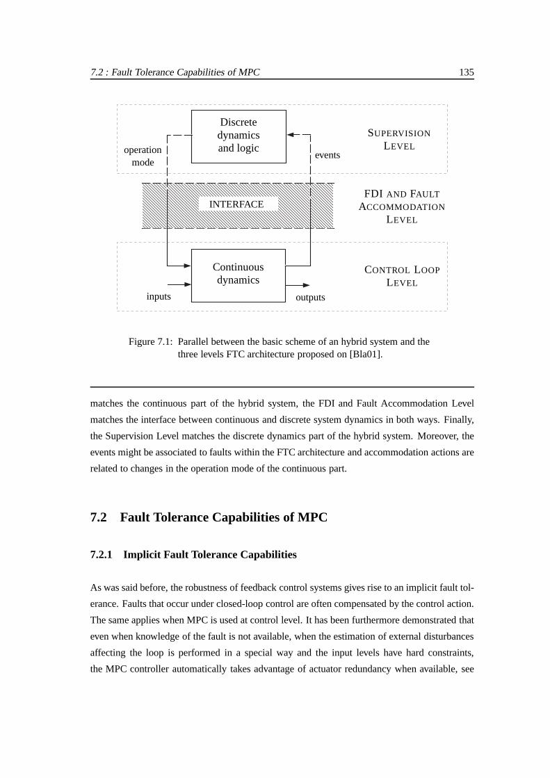
7.2 : Fault Tolerance Capabilities of MPC 135
xxxxxxxxxxxxxxxxxxxxxxxxxxxxxxxxxxxxxxxxxxxxxxxxxxxxxxxxxxxxxxxxxxxxxxxxxxxxxxxxxxxxxxxxxxxxxxxxxxxxxxxxxxxxxxxxxxxxxxxxxxxxxxxxxxxxxxxxxxxxxxxxxxxxxxxxxxxxxxxxxxxxxxxxxxxxxxxxxxxxxxxxxxxxxxxxxxxxxxxxxxxxxxxxxxxxxxxxxxxxxxxxxxxxxxxxxxxxxxxxxxxxxxxxxxxxxxxxxxxxxxxxxxxxxxxxxxxxxxxxxxxxxxxxxxxxxxxxxxxxxxxxxxxxxxxxxxxxxxxxxxxxxxxxxxxxxxxxxxxxxxxxxxxxxxxxxxxxxxxxxxxxxxxxxxxxxxxxxxxxxxxxxxxxxxxxxxxxxxxxxxxxxxxxxxxxxxxxxxxxxxxxxxxxxxxxxxxxxxxxxxxxxxxxxxxxxxxxxxxxxxxxxxxxxxxxxxxxxxxxxxxxxxxxxxxxxxxxxxxxxxxxxxxxxxxxxxxxxxxxxxxxxxxxxxxxxxxxxxxxxxxxxxxxxxxxxxxxxxxxxxxxxxxxxxxxxxxxxxxxxxxxxxxxxxxxxxxxxxxxxxxxxxxxxxxxxxxxxxxxxxxxxxxxxxxxxxxxxxxxxxxxxxxxxxxxxxxxxxxxxxxxxxxxxxxxxxxxxxxxxxxxxxxxxxxxxxxxxxxxxxxxxxxxxxxxxxxxxxxxxxxxxxxxxxxxxxxxxxxxxxxxxxxxxxxxxxxxxxxxxxxxxxxxxxxxxxxxxxxxxxxxxxxxxxxxxxxxxxxxxxxxxxxxxxxxxxxxxxxxxxxxxxxxxxxxxxxxxxxxxxxxxxxxxxxxxxxxxxxxxxxxxxxxxxxxxxxxxxxxxxxxxxxxxxxxxxxxxxxxxxxxxxxxxxxxxxxxxxxxxxxxxxxxxxxxxxxxxxxxxxxxxxxxxxxxxxxxxxxxxxxxxxxxxxxxxxxxxxxxxxxxxxxxxxxxxxxxxxxxxxxxxxxxxxxxxxxxxxxxxxxxxxxxxxxxxxxxxxxxxxxxxxxxxxxxxxxxxxxxxxxxxxxxxxxxxxxxxxxxxxxxxxxxxxxxxxxxxxxxxxxxxxxxxxxxxxxxxxxxxxxxxxxxxxxxxxxxxxxxxxxxxxxxxxxxxxxxxxxxxxxxxxxxxxxxxxxxxxxxxxxxxxxxxx
xxxxxxxxxxxxxxxxxxxxxxxxxxxxxxxxxxxxxxxxxxxxxxxxxxxxxxxxxxxxxxxxxxxxxxxxxxxxx
xxxxxxxxxxxxxxxxxxxxxx
xxxxxxxxxxxxxxxxxxxxxxxxxxx
xxxxxxx
xxxxxxxx xxxxxxx
Discretedynamicsand logicoperation
modeevents
SUPERVISION
LEVEL
INTERFACEFDI AND FAULT
ACCOMMODATION
LEVEL
inputs outputs
Continuousdynamics
CONTROL LOOP
LEVEL
Figure 7.1: Parallel between the basic scheme of an hybrid system and thethree levels FTC architecture proposed on [Bla01].
matches the continuous part of the hybrid system, the FDI andFault Accommodation Level
matches the interface between continuous and discrete system dynamics in both ways. Finally,
the Supervision Level matches the discrete dynamics part ofthe hybrid system. Moreover, the
events might be associated to faults within the FTC architecture and accommodation actions are
related to changes in the operation mode of the continuous part.
7.2 Fault Tolerance Capabilities of MPC
7.2.1 Implicit Fault Tolerance Capabilities
As was said before, the robustness of feedback control systems gives rise to an implicit fault tol-
erance. Faults that occur under closed-loop control are often compensated by the control action.
The same applies when MPC is used at control level. It has beenfurthermore demonstrated that
even when knowledge of the fault is not available, when the estimation of external disturbances
affecting the loop is performed in a special way and the inputlevels have hard constraints,
the MPC controller automatically takes advantage of actuator redundancy when available, see

136 Chapter 7 : Model Predictive Control and Fault Tolerance
[Mac98]. However, when the states are assumed measurable orestimable, this fault tolerance
property does not apply.
On the other hand, it is possible, when using the MPC formalism, to increase fault tolerance,
if knowledge of faults is available by modifying parametersof the optimization problem which
is solved in each sample. Faults that affect the internal model or system constraints can in this
way be incorporated into a MPC controller in a natural way. Furthermore, due to the flexibility
that control objectives can be expressed within the MPC formalism, when faults cause control
objectives to become unattainable, they can be dropped fromthe optimization problem or de-
graded in priority, for example, by changing hard constraints to soft ones. The information of a
fault occurrence can be included in a MPC law in the followingways:
• Changing the constraints in order to represent certain kinds of fault, being specially “easy”
to adapt the algorithms for faults in actuators.
• Modifying the internal plant model used by the MPC in order toreflect the fault influence
over the plant.
• Relaxing the initial control objectives in order to reflect the system limitations under fault
conditions.
However, these ways relies on several assumptions [Mac99]:
• The nature of the fault can be located and its effects modeled.
• The internal model of the plant can be updated, essentially in an automatic manner.
• The set of control objectivesO defined in the MPC design process can be left unaltered
once the fault has occurred.
These strong assumptions can be treated by using a reliable FDI an taking advantage of
the emerging technologies not only for system management but also for the friendly interaction
between the designer/user and the complex systems.
The idea of using FTC considering MPC as the control law of thetolerant architecture
has been reported in the literature during the last few years. The first steps on this field were
discussed in [Mac97] and the theory was implemented over an aircraft system in [MJ03]. The
main results reported allow to conclude, among other ideas,that MPC has a good degree of fault

7.2 : Fault Tolerance Capabilities of MPC 137
tolerance to some faults, especially actuator faults, under a certain conditions, even if the faults
are not detected. Subsequently, MPC and its advantages related to fault tolerance have inspired
other contributions to the FTC field, see [PMNS06], [AGBG06], [MVSdC06], among others.
In [PNP05], the authors propose an scheme where the fault tolerance and MPC work together
in chemical applications since MPC controllers are typically used to control key operations in
chemical plants, so this can have an impact on safety an productivity of the entire system. Based
the model predictive control, [Zho04] proposes a FTC designconsidering faults on actuator
elements. There, the simple fault detection and fault complement approach are presented and
discussed.
7.2.2 Explicit Fault Tolerance Capabilities
Linear constrained MPC is based on the solution of an optimization problem using either linear
or quadratic programming, which determines the optimal control action. As the coefficients of
the linear term in the cost function and the right hand side ofthe problem constraints depend
linearly on the current state, in particular the quadratic programming can be viewed as a mul-
tiparametric quadratic programming (mpQP). In [BMDP02], the authors analyze the properties
of mpQP, showing that the optimal solution is a piecewise affine function of the vector of pa-
rameters. As a consequence, the MPC controller is a piecewise affine control law which not
only ensures feasibility and stability, but also is optimalwith respect to LQR performance. An
algorithm based on a geometric approach for solving mpQP problems in order to obtain explicit
receding horizon controllers was proposed in [BMDP02].
The explicit form of the MPC controller provides also additional insight for better under-
standing the control policy. Moreover, this methodology allows introducing faults as additional
parameters into the parametric programming algorithms thanks to the information given by a
FDI module. For instance, in the case of faults affecting actuator bounds, since the maximum
control input from an actuator is often constrained in the optimization formulation, this con-
straint can be considered as a parameter. Thus, if an actuator has failed, the situation can be
handled by constraining the corresponding control input tobe null (reconfiguration strategy)
or, using the fault information available, by constrainingthe control related input to have the
new (faulty) operating ranges (accommodation). Example 7.1 allows to understand how a MPC
controller handles a fault situation.

138 Chapter 7 : Model Predictive Control and Fault Tolerance
Example7.1. Consider a first-order continuous system described by the transfer function
G(s) =0.8
2s + 1,
whose equivalent discrete-time state-space description,using a sampling time∆t = 0.1 s, is
given by
xk+1 = 0.9512xk + 0.0975uk
yk = 0.8xk
(7.1)
where|uk| ≤ µ andµ = 1. For notation proposes,uk ∈ [µ, µ] = [−1, 1]. It is clear that in this
case,−µ = µ. An MPC controller is used in the closed-loop system satisfying the associated
control constraints and considering the cost function
J(xk, uk) = Px2Hp
+
Hp−1∑
i=0
(Qx2
i +Ru2i
)(7.2)
whereHp = 2 and the terminal weight matrixP is determined using the Ricatti equation with
Q = 1 andR = 0.1. According to Theorem 6.2.1 in [GSdD05], since in this particular case the
prediction horizon is 2, the explicit form of the optimal control law u∗k = K2(x), which depends
on the current system statex0 = x, is given by1
K2(x) =
−satµ(Gx+ h) if x ∈ Z−
−satµ(Kx) if x ∈ Z
−satµ(Gx− h) if x ∈ Z+
(7.3)
where the saturation function satµ(·) is defined, for the saturation levelµ, as:
satµ(uk) =
µ if uk > µ
uk if |uk| ≤ µ−µ if uk < −µ
(7.4)
K andP are obtained by the algebraic Ricatti equation
P = ATPA+Q−KT (R +BTPB)K, K = (R+BTPB)−1BTA,
1Results used to show analytically the MPC fault tolerance capabilities are limited to be applied consideringHp = 2. Results related to mp-programming are more general.

7.2 : Fault Tolerance Capabilities of MPC 139
which givesP = 3.2419 andK = 2.2989 for the current example. Also from Theorem 6.2.1 in
[GSdD05], the gainG ∈ R1×n and the constanth ∈ R are given by
G =K +KBKA
1 + (KB)2and h =
KB
1 + (KB)2µ, (7.5)
which givesG = 2.6557 andh = 0.2135. The state space partitions for control law (7.3) are
defined by
Z− = x : K(A−BK)x < −µZ = x : |K(A−BK)x| ≤ µ
Z+ = x : K(A−BK)x > µ
(7.6)
which determines the following sets for the particular case:
Z− = x : 1.6713x < −µZ = x : 1.6713x ≤ µ
Z+ = x : 1.6713x > µ
In can be noticed that control law (7.3) depends indirectly of the actuator limits given by
µ, through expressions in (7.5) and (7.6). Therefore, it is clear how the effect of a fault over
the actuator operating range can modify the expression of control law. This suggests that (7.3)
can be parameterized in function of the actuator faults (limits). This parametrization is possi-
ble using results given in [BMDP02], where state-feedback explicit control law for the MPC
controller, piece-wise affine with respect to the states, can be derived using multiparametric
quadratic programming (mpQP). Using this approach in the current example, the expression of
K2(·) is given in function of the parametersθ = [ x µ µ ]T , which constitutes an extended
system composed by the system state and the control input bounds of its operating range. Thus,
expression
K2(θ) =
[−2.299 0 0 ] θ if[
1.6713 1 0−1.6713 0 −1
]θ ≤ [ 0
0 ]
(Region #1)
[−2.656 0 −0.2135 ] θ if[
0 1 −11.272 0 0.7611
]θ ≤ [ 0
0 ]
(Region #2)
[−2.656 −0.2135 0 ] θ if[
0 1 −1−1.272 −0.7611 0
]θ ≤ [ 0
0 ]
(Region #3)
(7.7)

140 Chapter 7 : Model Predictive Control and Fault Tolerance
System state
actuatorlower bound
actu
ator
uppe
rbo
und
Figure 7.2: Polyhedra partitions related to control law (7.7) for Example7.1.
corresponds to the explicit PWA control law, which has been obtained and represented graphi-
cally (see Figure 7.2) using the mp-programming tools included in the HYBRID TOOLBOX for
MATLAB r [Bem06]. Comparing expressions (7.3) and (7.7), it can be seen that both control
laws are equivalent.
7.3 Fault Tolerant Hybrid MPC
As discussed in Section 7.1, a FTC system matches an hybrid system. If an MPC controller
is used at Control Loop Level within the three-level architecture discussed before, in order to
take advantage of all fault tolerant capabilities described in this chapter, the use of Hybrid MPC
methodologies follows naturally in this framework. This section deals with the interaction of
blocks within a FTC scheme taking into account the hybrid modeling of the plant for the MPC
control proposes.
Looking at the schemes shown in Figures 7.3 and 7.4, which will be used in later sections
to explain the fault tolerant hybrid MPC strategies, it can be noticed that the plant is treated

7.3 : Fault Tolerant Hybrid MPC 141replacements
dt
fault
uℓ
uc
xck+1 = gc (xck,u, θck, dk)yck = hc (xck,u, θck, dk)
plant mode
EventGenerator
xp
xp = gp
(xpt, ut, θpt, dt
)
ypt = hp
(xpt, ut, θpt, dt
)ypyp
OPTIMIZER
ControllerPlant
Figure 7.3: Scheme of the PFTHMPC architecture.
as an hybrid system, where the continuous and discrete partsinteract using the event generator
interface. External effects such as disturbances and/or noise affect selectively parts of the plant.
Despite the faults can occur in any constitutive element within the system, they can be seen as
external events that affect the nominal behavior altering the system dynamics. Furthermore, the
closed-loop controller may apply either continuous or discrete inputs over the plant according
to its nature and to the control design. The following sections present the description of the fault
tolerant hybrid MPC strategies according to the available information related to the influence of
faults in an hybrid system model-based plant.
7.3.1 Fault Tolerant Hybrid MPC Strategies
The are two strategies in order to implement FTC using HybridMPC depending on the available
information about the existence of faults at the Control Loop Level. The definition of these
strategies follows the concepts and features described in Section 2.3.
In case of lacking of knowledge about the presence of the fault, the hybrid controller should
deal with a plant that has changed its mode because the fault effect. In this case, fault tolerance
relies on the implicit tolerance capabilities of the feedback control loop. This strategy is called
in the sequel as Passive FTHMPC (PFTHMPC). Figure 7.3 shows aconceptual scheme of this
strategy.

142 Chapter 7 : Model Predictive Control and Fault Tolerance
plant statusinformation
FDISUPERVISOR(Automaton)
controlmode
dt fault
uℓ
uc
u =
[uc
uℓ
]
xck+1 = gc (xck,u, θck, dk)yck = hc (xck,u, θck, dk)
plant mode
EventGenerator
xp
xp = gp
(xpt, ut, θpt, dt
)
ypt = hp
(xpt, ut, θpt, dt
)ypyp
OPTIMIZER
Controller Plant
Figure 7.4: Scheme of the AFTHMPC architecture.
On the other hand, in the case of having knowledge about the presence of the fault thanks
to the existence of an FDI module, the hybrid controller can adapt its operation mode in order
to handle the faulty plant operating mode. In this case faulttolerance take advantage of the
the implicit fault tolerant capabilities of MPC as described before. This strategy is called in
the sequel as Active Fault Tolerant Hybrid Model PredictiveControl (AFTHMPC). Figure 7.4
shows a conceptual scheme of this strategy. Notice that FDI module functionality is assumed to
work correctly. Ideally, it detects and isolates the faultyactuator and returns the corresponding
information complemented with the fault magnitude. The fault information is assumed readily
available and is used to modify the corresponding constraints in the optimization problem.
7.3.2 Active Fault Tolerant Hybrid MPC
Once the “fault tolerant loop” is closed with the FDI module and the Supervisor, the whole FTC
system starts an exchange of signals of different nature andobjective, following the operating
philosophy of a generic hybrid system.
From the plant, continuous and discrete signals are received in the FDI module which are

7.4 : Fault Tolerant Hybrid MPC on Sewer Networks 143
complemented with signals of both natures from the controller. This mixture of information
is processed by the algorithms of diagnosis obtaining the plant status information: nominal or
faulty; if faulty, where the fault is, its magnitude, etc. The status information is then sent to the
Supervisor, which takes the corrective actions related to the fault occurrence. The supervisor
block within a FTC architecture is considered in itself a state machine, which implies again an
hybrid behavior within the fault tolerance loop. The information given by FDI algorithms is then
processed by the supervisor, which determines several aspects of the closed-loop system status
and modifies the control law in order to respond facing the fault event. The joint design of the
supervisor and control strategy blocks (what is usually done) using hybrid modeling techniques
gets high compatibility due to the same nature of their structures.
However, each fault type induces different dynamics in the plant. In the set of the operating
plant modes, a new subset of “faulty modes” would be added. Try to define all these faulty
dynamics and/or plant operating modes taking into account the fault influence could be a hard
work and sometimes an impossible mission. In this sense, an plant hybrid modeling would have
to include an complementary model which incorporates the hybrid model representation of the
fault effects for a given set of fault scenarios.
In the same way, a compositional hybrid system [Joh00] wouldhave to consider the hybrid
model for each constitutive element where the inherent continuous and discrete dynamics and
the fault influences are taken into account simultaneously.The main disadvantage of this ap-
proach could lie on the high dimension of the logical dynamics, what produces a combinatorial
effect in the continuous dynamics. Consider a system represented with a MLD form. The inclu-
sion of the hybrid modeling of the considered faults can increase the dimension ofδ variables,
what yields a more complex MIP in the design process of the HMPC closed-loop (see Chapter
5). Considering this phenomena, the suboptimal strategiesdiscussed and proposed in Chapter 6
are now an alternative way to deal with these limitations.
7.4 Fault Tolerant Hybrid MPC on Sewer Networks
In this chapter, Fault Tolerant Hybrid MPC strategy (FTHMPC) strategy on sewer networks
just considers actuator faults as the change of the bounds ofthe operating ranges related to
input signals,qui
andqui, in the discrete optimization problem solved online. This information
would be available once the FDI has detected, isolated and estimated the actuator fault occurred
in the sewage system. According to the ideas discussed in previous sections, the FTHMPC

144 Chapter 7 : Model Predictive Control and Fault Tolerance
is now implemented and tested over the BTC. This section presents the typical fault scenarios
occurred on control gates of sewer networks and discusses the modeling of these phenomena
in the hybrid systems framework. The use of the hybrid approach is motivated by the results
obtained in a previous study where faults were considered within a linear MPC design. To
motivate the fault tolerant approach, results are presented making a comparison between the
FTHMPC strategies. As was said before, the functionality ofthe associated FDI module in the
AFTHMPC strategy is assumed to work correctly. It detects and isolates the faulty actuator
and returns the corresponding information complemented with the fault magnitude. The fault
information is assumed readily available and is used to modify the corresponding constraints in
the discrete optimization problem.
7.4.1 Considered Fault Scenarios
There may exists many types of fault scenarios related to thecontrol gates within a sewer net-
work. During this chapter, three fault scenarios are considered since they might represent the
typical phenomena occurred with these elements under common faulty conditions for these sys-
tems and taking into account that the control signal is the outflow rate from the control gates.
The flow range can be limited from below due to the inability toclose a gate and it can be lim-
ited from above due to the inability to open a gate sufficiently (or reduction in pump capacity
if pumping elements were considered). A stuck gate means therange is limited to a point or
very narrow interval. Hence, the fault scenarios consist inlimiting the range of the gates in three
ways:
1. Limit range from below (range is 50-100%), denoted asfqui
.
2. Limit range from above (range is 0-50%), denoted asfqui.
3. Limit from below and above, simulating stuck gate (50-51%) and denoted asfqui
.
In scenarios 1 and 3,qui
= 0.5 qui. For the BTC in Figure 5.6 and particularly in scenario
fqu2
, the lower limit of gateC2, qu2
, was set equal to the upper limit of actuatorC3, qu3. The
reason for this arrangement is that the optimization problem is infeasible if tankT2 is full and
qu2
> qu3.

7.4 : Fault Tolerant Hybrid MPC on Sewer Networks 145
7.4.2 Linear Plant Models and Actuator Faults
When the internal model of the predictive controller is considered as in Chapter 4, i.e., a linear
model, the AFTMPC strategy deals with a optimization problem whose convexity is given by
the type of fault considered. Assuming that any fault model modifies the upper limit for any
actuator range, the optimization problem can be solved using fast algorithms of linear program-
ming (LP) in the case of cost function with linear norms or quadratic programming (QP) in the
case of quadratic norms. This issue makes that the approach can deal with big systems having
many state variables, what yields relative big optimization problems that can be solve very fast
obtaining the global optimal solution. Notice that under these conditions, the problem can be
easily scalable in the sense of the sewer network size.
However, when the fault effect makes that at least one of the ranges for any system actu-
ator has a nonzero lower bound, the constraint related to this actuator is now non-convex and
therefore the optimization problem is non-convex as well. In this case, it is not possible to take
advantage of the LP or QP algorithms to solve the optimization problem and its solution is not
global (suboptimal). This problem is reported in [OMPQI05], where a small system inspired on
the BTC was used. The proposed system contains representative elements of the whole sewer
network of Barcelona and considers components enough for testing the FTC strategies based
on MPC. The results obtained shown the usefulness of the fault tolerant approach when certain
models of faults are considered, including models wherequi
is nonzero. Nevertheless, with
fault models modifyingqui
, the obtained solution corresponded to a local minimum of the cost
function, which implies that the approach performance is just suboptimal.
7.4.3 Hybrid Modeling and Actuator Faults
The ideas proposed in [OMPQI05] and discussion in Section 7.3 motivates to explore other al-
ternatives of modeling for the considered fault scenarios taking advantage of techniques having
a desirable level of accuracy in the expression of the complex dynamics of the system. Hence,
this chapter uses the hybrid systems modeling presented in Chapter 5 to take into account ac-
tuator faults in sewer networks considering the three faultscenarios as modes related to the
behavior of the element. Figure 7.5 shows a conceptual behavior of the system once the fault
has occurred. Notice that the system changes between different modes depending on the fault
scenario. In this case, it is considered that single fault affects the system. Two or more faults at
same time causes here a explosion in the amount of system modes.

146 Chapter 7 : Model Predictive Control and Fault Tolerance
...
other faultscenarios
faultscenario 1
faultscenario 2
faultscenario 3
NM
F1
F2
F3
Figure 7.5: Conceptual scheme of actuator mode changing considering faultscenarios. NM denotes the nominal (non-faulty) actuator mode.
qin
qui
qb
Figure 7.6: Control gate scheme used to explain the fault hybrid modeling.
For instance, consider the fault actuator modefqui
for the redirection gate presented in
Figure 5.3, which is repeated here for simplicity. In this case, it is shown how such mode can be
expressed using the proposed hybrid modeling approach2.
This fault limits explicitly the range of the manipulated outflow qui. Then, the following
2Similarly, the rest of fault modes described in Section 7.4.1 can be modeled using this approach.

7.4 : Fault Tolerant Hybrid MPC on Sewer Networks 147
expressions are obtained using the principle of mass conservation:
qui≤ min(qui
, qin) (7.8a)
qui≥ min(q
ui, qin). (7.8b)
which derives in non-convex constraints on the optimization problem. It can be noticed that this
behavior is similar to the switching behavior associated toweirs and suggests the appearance
of new system modes. This fact further motivates the use of the proposed hybrid modeling
methodology.
Inequality (7.8a) related to the upper bound can be expressed with two linear inequalities
as:
qui≤ qui
, qui≤ qin.
Notice that in the case of fault scenariosfquiand fq
ui, the fault affects the system when
qin > fqui. Otherwise, the fault does not have any influence over the behavior of the net-
work.
The non-convex constraint (7.8b) can be easily treated in the hybrid framework by introduc-
ing auxiliary variables
[δi = 1]→ [qui≤ qin] (7.9a)
zqui=
qui
if δi = 1
qin otherwise(7.9b)
and replacing (7.8b) by qui≥ zqui
. In this way, a non-convex constraint can be expressed with a
finite number of linear constraints in the optimization problem (using the equivalences (5.1) and
(5.2)), avoiding possible problems due to convergence of optimization routines to local minima.
Figure 7.7 shows the set of valid values forquiwhere the actuator constraints are fulfilled.
Notice the change of the area when the boundqui
is modified due to the fault effect. Also notice
that whenqui
is nonzero, points over the line defined byqui= qin and (7.8a) belong to that set
of valid values.
This fault modeling associated with the hybrid approach forsewer network elements suggest
that each element can include typical fault models according to its nature within the network.
Hence, the fault tolerance is included in the modeling process when the MPC plant model is

148 Chapter 7 : Model Predictive Control and Fault Tolerance
xxxxxxxxxxxxxxxxxxxxxxxxxxxxxxxxxxxxxxxxxxxxxxxxxxxxxxxxxxxxxxxxxxxxxxxxxxxxxxxxxxxxxxxxxxxxxxxxxxxxxxxxxxxxxxxxxxxxxxxxxxxxxxxxxxxxxxxxxxxxxxxxxxxxxxxxxxxxxxxxxxxxxxxxxxxxxxxxxxxxxxxxxxxxxxxxxxxxxxxxxxxxxxxxxxxxxxxxxxxxxxxxxxxxxxxxxxxxxxxxxxxxxxxxxxxxxxxxxxxxxxxxxxxxxxxxxxxxxxxxxxxxxxxxxxxxxxxxxxxxxxxxxxxxxxxxxxxxxxxxxxxxxxxxxxxxxxxxxxxxxxxxxxxxxxxxxxxxxxxxxxxxxxxxxxxxxxxxxxxxxxxxxxxxxxxxxxxxxxxxxxxxxxxxxxxxxxxxxxxxxxxxxxxxxxxxxxxxxxxxxxxxxxxxxxxxxxxxxxxxxxxxxxxxxxxxxxxxxxxxxxxxxxxxxxxxxxxxxxxxxxxxxxxxxxxxxxxxxxxxxxxxxxxxxxxxxxxxxxxxxxxxxxxxxxxxxxxxxxxxxxxxxxxxxxxxxxxxxxxxxxxxxxxxxxxxxxxxxxxxxxxxxxxxxxxxxxxxxxxxxxxxxxxxxxxxxxxxxxxxxxxxxxxxxxxxxxxxxxxxxxxxxxxxxxxxxxxxxxxxxxxxxxxxxxxxxxxxxxxxxxxxxxxxxxxxxxxxxxxxxxxxxxxxxxxxxxxxxxxxxxxxxxxxxxxxxxxxxxxxxxxxxxxxxxxxxxxxxxxxxxxxxxxxxxxxxxxxxxxxxxxxxxxxxxxxxxxxxxxxxxxxxxxxxxxxxxxxxxxxxxxxxxxxxxxxxxxxxxxxxxxxxxxxxxxxxxxxxxxxxxxxxxxxxxxxxxxxxxxxxxxxxxxxxxxxxxxxxxxxxxxxxxxxxxxxxxxxxxxxxxxxxxxxxxxxxxxxxxxxxxxxxxxxxxxxxxxxxxxxxxxxxxxxxxxxxxxxxxxxxxxxxxxxxxxxxxxxxxxxxxxxxxxxxxxxxxxxxxxxxxxxxxxxxxxxxxxxxxxxxxxxxxxxxxxxxxxxxxxxxxxxxxxxxxxxxxxxxxxxxxxxxxxxxxxxxxxxxxxxxxxxxxxxxxxxxxxxxxxxxxxxxxxxxxxxxxxxxxxxxxxxxxxxxxxxxxxxxxxxxxxxxxxxxxxxxxxxxxxxxxxxxxxxxxxxxxxxxxxxxxxxxxxxxxxxxxxxxxxxxxxxxxxxxxxxxxxxxxxxxxxxxxxxxxxxxxxxxxxxxxxxxxxxxxxxxxxxxxxxxxxxxxxxxxxxxxxxxxxxxxxxxxxxxxxxxxxxxxxxxxxxxxxxxxxxxxxxxxxxxxxxxxxxxxxxxxxxxxxxxxxxxxxxxxxxxxxxxxxxxxxxxxxxxxxxxxxxxxxxxxxxxxxxxxxxxxxxxxxxxxxxxxxxxxxxxxxxxxxxxxxxxxxxxxxxxxxxxxxxxxxxxxxxxxxxxxxxxxxxxxxxxxxxxxxxxxxxxxxxxxxxxxxxxxxxxxxxxxxxxxxxxxxxxxxxxxxxxxxxxxxxxxxxxxxxxxxxxxxxxxxxxxxxxxxxxxxxxxxxxxxxxxxxxxxxxxxxxxxxxxxxxxxxxxxxxxxxxxxxxxxxxxxxxxxxxxxxxxxxxxxxxxxxxxxxxxxxxxxxxxxxxxxxxxxxxxxxxxxxxxxxxxxxxxxxxxxxxxxxxxxxxxxxxxxxxxxxxxxxxxxxxxxxxxxxxxxxxxxxxxxxxxxxxxxxxxxxxxxxxxxxxxxxxxxxxxxxxxxxxxxxxxxxxxxxxxxxxxxxxxxxxxxxxxxxxxxxxxxxxxxxxxxxxxxxxxxxxxxxxxxxxxxxxxxxxxxxxxxxxxxxxxxxxxxxxxxxxxxxxxxxxxxxxxxxxxxxxxxxxxxxxxxxxxxxxxxxxxxxxxxxxxxxxxxxxxxxxxxxxxxxxxxxxxxxxxxxxxxxxxxxxxxxxxxxxxxxxxxxxxxxxxxxxxxxxxxxxxxxxxxxxxxxxxxxxxxxxxxxxxxxxxxxxxxxxxxxxxxxxxxxxxxxxxxxxxxxxxxxxxxxxxxxxxxxxxxxxxxxxxxxxxxxxxxxxxxxxxxxxxxxxxxxxxxxxxxxxxxxxxxxxxxxxxxxxxxxxxxxxxxxxxxxxxxxxxxxxxxxxxxxxxxxxxxxxxxxxxxxxxxxxxxxxxxxxxxxxxxxxxxxxxxxxxxxxxxxxxxxxxxxxxxxxxxxxxxxxxxxxxxxxxxxxxxxxxxxxxxxxxxxxxxxxxxxxxxxxxxxxxxxxxxxxxxxxxxxxxxxxxxxxxxxxxxxxxxxxxxxxxxxxxxxxxxxxxxxxxxxxxxxxxxxxxxxxxxxxxxxxxxxxxxxxxxxxxxxxxxxxxxxxxxxxxxxxxxxxxxxxxxxxxxxxxxxxxxxxxxxxxxxxxxxxxxxxxxxxxxxxxxxxxxxxxxxxxxxxxxxxxxxxxxxxxxxxxxxxxxxxxxxxxxx
0
0
qin (m3/s)
qu
i(m
3/s
)
qui
qui
qui
Figure 7.7: Values forquiwhere actuator constraints are fulfilled.
obtained, assuming that the fault information is provide bya FDI module. This feature allows to
have a more accurate representation of the real plant when a given fault effect is considered and
makes easier the reconfiguration/accommodation of the control law within the FTC architecture.
Another advantage of the fault hybrid modeling lies on the possibility of having continuity in
the fault magnitude for a given particular fault model. Thisfact also increases the accuracy of
the element model facing fault occurrence.
7.4.4 Implementation and Results
The purpose of this section lies on comparing AFTHMPC and PFTHMPC for realistic episodes
of rain storms (Section 3.3.3) and actuator faults (Sections 7.4.1) for the BTC in Figure 5.6. The
assumptions made for the comparison will be presented and their validity discussed before the
results are given. In all cases, fault accommodation has been done. For this particular case study,
the reconfiguration strategy would consist in considering the control gate totally open when a
actuator fault occurs. Thus, the sewage flows downstream by the gravity action fulfilling the
mass conservation principle and respecting the main paths.However, notice that this behavior
occurs when fault scenarios with nonzero lower bound on the operational ranges are considered.

7.4 : Fault Tolerant Hybrid MPC on Sewer Networks 149
This observation is valid while the gate inflow is lower than the faulty lower bound.
Simulation of Scenarios
The control strategies were compared by simulating the closed-loop system for all fault scenar-
ios presented in Section 7.4.1 and for the rain episodes listed in Table 3.3. The structure of the
closed-loop is the same as the one performed for simulationsin Chapter 5. In the PFTHMPC
case, the actuator ranges were limited only in the plant model.
The duration of the simulations scenarios was selected to have 8 hours approximately (k ∈[0, 100]) as the rain storm generally had peaks of duration around 10 samples or 50 minutes.
The tanks were empty in the beginning of the scenarios. To compare strategies, total flooding,
pollution and treated water released was added over the whole scenario.
The prediction horizonHp and control horizonHu were selected as 6 samples or 30 minutes
for reasons given in previous chapters. The cost function structure, norm and control tuning
used were the same as in the simulations done for nominal HMPCshown in Chapter 5 and the
software tools for simulation as well as the solver package were the same as well.
Main Results
Generally, CSO flooding in streets was reduced when AFTMPC was used compared to
PFTMPC. The biggest improvements were obtained when precipitation was large enough so
that actuators needed to operate close to the upper limit of their range, that is when the pre-
cipitation brought the sewer network close to its capacity.Even though results are shown for
specific rain episodes, the conclusions presented were based on simulation of various scenarios.
AFTMPC did not yield great improvements when heavy rain episodes as the one occurred on
September 14, 1999 (see Figure 3.8(a)) was considered in thesimulation. The reduction in CSO
that could be achieved was about 0-5%. The reason for this is that the BTC does not have the
capacity to handle rain storms with that intensity even in the fault free case. Therefore, it did not
matter if actuation limits were known to the HMPC controlleror not. This behavior can be seen
in Table 7.1 where the main performance indices for the BTC were compared for the considered
fault scenarios using AFTHMPC and PFTHMPC. Notice that the largest flooding reduction was
obtained for scenariosfqu2andfq
u2
. There the flooding was reduced from roughly 135700 m3
to around 121000 m3, which corresponds to an improvement about 11%. The other performance

150 Chapter 7 : Model Predictive Control and Fault Tolerance
Table 7.1: Results for FTHMPC with rain episode occurred on September14, 1999.
Fault Scenario PFTHMPC AFTHMPC
Actuator TypeFlooding Pollution Treated W. Flooding Pollution Treated W.×103 (m3) ×103 (m3) ×103 (m3) ×103 (m3) ×103 (m3) ×103 (m3)
fqu1
99.5 223.5 280.6 99.5 223.5 280.6qu1
fqu193.6 223.9 280.3 93.4 223.8 280.3
fqu1
99.9 223.9 280.3 99.9 223.9 281.6
fqu2
92.9 222.7 281.5 92.9 222.7 281.5qu2
fqu2135.7 230.2 274.1 121.0 228.8 275.5
fqu2
125.5 226.6 277.6 118.3 227.5 276.7
fqu3
94.3 226.0 278.2 94.2 225.3 278.9qu3
fqu397.7 221.1 283.2 95.1 223.1 281.0
fqu3
97.6 223.1 281.2 96.0 224.7 279.5
fqu4
102.1 222.4 281.8 102.1 222.3 281.9qu4
fqu492.8 223.5 280.7 92.8 223.5 280.7
fqu4
102.1 222.4 281.8 102.1 222.3 281.9
indices were also improved simultaneously. It can occur that flooding was reduced but pollution
and/or treated water were not. This fact is caused by the objective prioritization reflected in the
tuning of the cost function. However, pollution and floodingindices were improved as well as
the flooding was also improved.
When very common rain episodes with little precipitation were studied the same thing oc-
curred, that is, AFTMPC did not give a great improvement. Thereason for this is that in those
scenarios the constraints are usually not reached and thus faults in actuators rarely affect perfor-
mance.
Results are shown in Table 7.2 for a rain storm occurred on October 17, 1999. This rain
episode has a 0.7-year return period with regard to total amount and 10-year return period with
regard to maximum intensity. The particular feature of thisepisode lies on its behavior during
the time window considered. As was seen in Figure 3.8(b), this rain presents a double peak of
intensity, what yields that the sewer network behavior is more complex and the nominal HMPC
and the FTHMPC designs have a lot of work trying to control thesystem and avoiding the
fault influence. The network is almost not sensitive to faults in gatesC1 andC4. The modified
upper bounds forqu1andqu4
were always greater than the inflow of the corresponding control

7.4 : Fault Tolerant Hybrid MPC on Sewer Networks 151
Table 7.2: Results for FTHMPC with rain episode occurred on October 17,1999.
Fault Scenario PFTHMPC AFTHMPC
Actuator TypeFlooding Pollution Treated W. Flooding Pollution Treated W.×103 (m3) ×103 (m3) ×103 (m3) ×103 (m3) ×103 (m3) ×103 (m3)
fqu2
0.0 61.9 291.4 0.0 61.9 291.4qu2
fqu215.9 62.8 290.5 10.4 63.3 290.0
fqu2
14.8 63.3 290.0 9.6 63.8 289.5
fqu3
0.0 59.1 294.2 0.0 58.8 294.5qu3
fqu33.5 57.7 295.6 0.2 58.7 294.7
fqu3
0.8 58.8 294.6 0.0 58.9 294.4
gates. Due to restrictions in lower bounds caused by the faults on these gates, the values for
manipulated flowsqu1andqu4
took the same values of the respective inflows in most of the
cases. Those values were not big enough to cause overflows downstream.
In this case, the most representative flooding reduction occurred in the fault scenariofqu2,
with about 35% of improvement caused by the use of the AFTHMPCstrategy respect to the
PFTHMPC. This improvement is reached by means of a set of procedures caused by the com-
puted control signals. Figure 7.8 shows this set of actions after the second rain peak for different
parts of the BTC for both active and passive approaches. In the active case and due to the ma-
nipulated flowqu2has lost capacity, the controller can not take advantage of the the real tankT3
in a short/medium term3. This fact induces that sewage coming fromT1 is conveniently derived
through sewerq14 (see Figure 7.8, top graph), what produces that sewers closetoT3 do not have
as much overflow as in the case of applying the passive strategy (see Figure 7.8, medium graph).
The slow filling ofT3 plus its convenient outflow manipulation (control signal related toqu3, see
bottom graph in Figure 7.8) make that a bit of buffer capability benefits the overflow avoidance
in T5. All these actions produce the mentioned improvement of flooding reduction for this fault
scenario in this rain episode.
Finally, an intermediate type of rain episode in the sense ofrain intensity is for instance the
one occurred on September 3, 1999. This episode is well supported by the network topology
design, i.e., implementing an adequate control law, the sewer network would not have CSO.
Results obtained for this rain episode have shown that the network is almost not sensitive to
3Keep in mind that real tanks (reservoirs) are generally usedas a buffer within the network. Using this capability,they can store enough water to avoid flooding and/or CSO downstream.

152 Chapter 7 : Model Predictive Control and Fault Tolerance
30 40 50 60 70 80 90 1000
2
4
6
30 40 50 60 70 80 90 1000
5
10
30 40 50 60 70 80 90 1000
2
4x 10
4
time (samples)
volu
meT
3
over
flow
inq 2
4flo
winq 1
4
Figure 7.8: Set of actions in different parts of the BTC for both active andpassive FTHMPC approaches for fault scenariofqu2
. Solidcurve (−): PFTHMPC; dashed curve (−−): AFTHMPC;dotted-dashed curve (− · −): no-fault HMPC (rain episode:99-10-17).
all the considered fault scenarios in control gatesC1 andC4 due to the same reasons discussed
for the previous rain episode. Table 7.3 collects the results obtained for the other two actuators
where the AFTHMPC yielded improvements respect to the PFTHMPC strategy. In the scenarios
fqu3andfq
u3
, the FTC strategy achieved around 100% of flooding reduction. The reason of
this improvement is because the AFTHMPC takes advantage of the sewage accumulation in the
real tank imposed by the emptying restriction due to the fault (see medium graph in Figure 7.9)
and computes adequately the set of control signals in order to redirect the sewage avoiding big
quantities around the faulty elements within the sewer network.
When the PFTHMPC strategy is used, the controller computes acontrol signalqu3(k) with-
out knowing the fault in the actuator, which implies that thecomputed control signal and the

7.5 : Summary 153
Table 7.3: Results for FTHMPC with rain episode occurred on September3, 1999.
Fault Scenario PFTHMPC AFTHMPC
Actuator TypeFlooding Pollution Treated W. Flooding Pollution Treated W.×103 (m3) ×103 (m3) ×103 (m3) ×103 (m3) ×103 (m3) ×103 (m3)
fqu2
0.0 44.3 232.3 0.0 44.3 232.3qu2
fqu215.2 44.5 232.1 12.2 44.7 231.9
fqu2
14.7 44.3 232.3 11.8 44.4 232.2
fqu3
0.0 45.2 231.4 0.0 45.2 231.4qu3
fqu34.1 44.1 232.5 0.2 44.3 232.3
fqu3
1.5 44.3 232.3 0.0 44.3 232.3
applied signal related to the control action will be different (notice that the applied signal in
this case corresponds to the computed signal but saturated according to the faulty upper limit).
Hence, due to the physical constraints impose a limit on the real tank inflow (manipulated link
qu2) in function of its actual volume, sewage that enters inC2 is derived through sewerq24
causing overflow in this element and then flooding increase.
On the other hand, the AFTHMPC strategy computes the controlsignalqu1(k) in such a
way that the sewage fromT1 is redirected throughq14 and then less water goes towards the real
tank and its faulty output actuator. Thus, despite the slow emptying ofT3, theC2 water inflow is
conveniently distributed between sewersqu2andq24, avoiding the overflow in this latter sewer
and therefore preventing the flooding increase. Figure 7.9 shows the obtained signals related to
the computed control signalqu3(k) (top graph), the volume inT3 (medium graph) and overflow
in q24 (bottom graph) using both active and passive FTC strategies.
7.5 Summary
This chapter introduces concepts and methods to incorporate fault tolerance in a closed-loop
governed by an MPC control law. The both implicit and explicit fault tolerance capabilities of
this control technique has been outlined and particular features in this sense have been discussed.
Moreover, MPC designs considering hybrid system models areincluded in the framework of the
FTC. In fact, it has been proposed a parallelism between the conceptual structure of an hybrid
system and the three-levels FTC architecture. This proposal states that both conceptual schemes

154 Chapter 7 : Model Predictive Control and Fault Tolerance
0 20 40 60 80 1000
2
4
6
8
0 20 40 60 80 1000
2
4x 10
4
0 20 40 60 80 1000
2
4
6
time (samples)
q u3
volu
meT
3
over
flow
inq 2
4
Figure 7.9: Stored volumes in real tankT3 for fault scenariofqu3. Solid
curve (−), PFTHMPC, dashed curve (−−), AFTHMPC,dotted-dashed curve (− · −), no-fault HMPC (rain episode:03-09-1999).
match in the sense of signal natures and exchange between modules status information.
Within the hybrid MPC theory, two FTC strategies have been proposed to deal with faults.
The difference between them lies on the available information in the controller related to the
fault effects over the plant. The strategies proposed follow the philosophy discussed in Chapter
2 for control loop strategies in a FTC architecture.
Moreover, this chapter has presented a comparison between AFTHMPC and PFTHMPC
applied to sewer networks under realistic rain and fault scenarios. The result showed that AF-
THMPC reduces CSO flooding in almost all cases. Furthermore,using AFTHMPC could pre-
vent flooding or reduce it considerably when rain episodes considered are supported by the

7.5 : Summary 155
sewer network maintaining inside of its design limits. However, the performance is poorly im-
proved for heavy rains due to sewer network topological limitations. In the other extreme cases,
i.e., having light rains, the considered fault scenarios donot have an important influence on the
sewer network behavior due to the small internal flows handled.
The study presented motivates the use of FDI algorithms to diagnose actuator faults in sewer
networks. The diagnosis algorithm would provide the limitson the actuator range to be useful
for FTC.

156 Chapter 7 : Model Predictive Control and Fault Tolerance

CHAPTER 8
ACTUATOR FAULT TOLERANCE
EVALUATION
8.1 Introduction
In this chapter, fault tolerant evaluation of a certain actuator fault configuration (AFC) con-
sidering a linear predictive/optimal control law with constraints is studied. This problem has
been already treated in the literature for the case of LQR problem without constraints [Sta03],
due to the existence of analytical solution. However, constraints (on states and control signals)
are always present in real industrial control problems and could be easily handled using Linear
Constrained Model Predictive Control (LCMPC) [Mac02]. Butin general, an analytical solu-
tion for obtaining these control laws does not exist, which makes difficult the application of this
approach.
The method proposed in this chapter is not of analytical but of computational nature. It
follows the idea proposed by [LP04] in which the computationof the control law for a predic-
tive/optimal controller with constraints can be divided intwo steps: first, the computation of
solutions set that satisfies the constraints (feasible solutions) and second the optimal solution
determination.
Faults in actuators would cause important changes in the setof feasible solutions since
constraints on the control signals have varied. This causesthat the set of admissible solutions
for the given control objectives could be empty. Therefore,the admissibility of the control law
facing actuator faults can be determined knowing the feasible solutions set. One of the aims of
this chapter is to provide methods to compute this set and then evaluate the admissibility of the
157

158 Chapter 8 : Actuator Fault Tolerance Evaluation
control law.
To find the feasible solutions set for the LCMPC problem, a constraints satisfaction problem
could be formulated [LP04]. However, such problems are computationally demanding, what
induces to find a approximate solution bounded by interval hulls and in a iterative manner on
time. Proceeding in this way, an interval simulation problem is implicitly solved appearing
typical difficulties associated with it (such as wrapping effect, among others) [PSQ03]. In order
to avoid such problems, the region of possible states could be approximated using more complex
domains than intervals, such as subpavings [KJW02], ellipsoids [EC01, PSN+04], zonotopes
[Kuh98, ABC05], among others.
Therefore, this chapter presents a preliminary study aboutthe mentioned admissibility eval-
uation of AFC considering linear plant models. This study can be extended to the cases where
nonlinear or linear hybrid models are considered. First approximations by the way of nonlin-
ear systems are reported in [OMPQ06] while in the hybrid systems framework are reported in
[Tor03].
8.2 Preliminary Definitions
Considering the MPC problem defined in Section 2.2.1, and especially the sequencesuk andxk
in (2.2) and (2.4), respectively, the definitions below are given.
Definition 8.1 (Feasible solutions set). The feasible solutions set is given by
Ω = xk,uk |xk+1 = g(xk,uk)
and corresponds to the input and state sets that satisfy the system constraints.
Definition 8.2 (Feasible control objectives set). The feasible control objectives set is given by
JΩ = J(xk,uk) ∈ R | (xk,uk) ∈ Ω
and corresponds to the set of all values ofJ obtained from feasible solutions set.
In the case of a fault,Ω changes toΩf andJΩ changes toJΩf.
Definition 8.3 (Admissible solutions set). Given the following subsets:

8.3 : Admissibility Evaluation Approaches 159
• Ωf , defined as the feasible solutions set of a AFC and
• JA, defined as the admissible control objectives set,
the admissible solutions set is given by
A =xk,uk ∈ Ωf | J(xk,uk) ∈ JA ∩ JΩf
and corresponds to the feasible solutions subset that produces control objectives inJA. If A is
the empty set, then the considered AFC is not fault tolerant.
Definition 8.4 (Predicted states set). Given the set of states at timek-1, the set of predicted
states at timek is defined as:
Xpk = xk = g(xk−1, uk−1) |xk−1 ∈ Xk−1, uk−1 ∈ U
and corresponds to the set of states at timek originated by the system evolution starting from
the set of states at timek-1.
Definition 8.5 (Feasible states set). The set of feasible states at timek is given by
Xck =
xk |xk ∈ X
pk ∩X
and corresponds to the set of predicted states that satisfiesthe system state constraints.
Definition 8.6 (Admissible inputs set). The set of admissible inputs at timek-1 is given by
Uck−1 =
uk−1 ∈ U | (xk = g(xk−1, uk−1)) ∈ X
ck, xk−1 ∈ X
ck−1
and corresponds to the set of inputs that produces the set of feasible states.
Remark8.1. Notice thatUck−1 in Definition 8.6 is an alternative form for expressing the admis-
sible input sequence in (2.3).
8.3 Admissibility Evaluation Approaches
8.3.1 Admissibility Evaluation using Constraints Satisfaction
This section deals with the methodology proposed in order toevaluate the admissibility of a
given AFC by means of the constraint satisfaction approach.First of all, the definition of the

160 Chapter 8 : Actuator Fault Tolerance Evaluation
constraint satisfaction problem is presented and some particular details related to this approach
are presented and discussed. Then, this approach is explained in the framework of the AFC
admissibility evaluation.
Constraints Satisfaction Problem
A Constraints Satisfaction Problem(CSP) on sets can be formulated as a 3-tupleH = (Υ,Λ,C)
[JKBW01], where:
• Υ = υ1, · · · , υn is a finite set of variables,
• Λ = Λ1, · · · ,Λn is the set of their domains represented by closed sets and
• C = c1, · · · , cn is a finite set of constraints relating variables ofΥ.
A point solution ofH is a n-tuple(υ1, · · · , υn) ∈ Λ such that all constraintsC are satisfied.
The set of all point solutions ofH is denoted byS(H). This set is called theglobal solution set.
The variableυi ∈ Υi is consistentinH if and only if
∀υi ∈ Υi ∃ (υ1 ∈ Λ1 · · · , υn ∈ Λn) |(υ1, · · · , υn) ∈ S(H)
with i = 1, . . . , n. The solution of a CSP is said to beglobally consistent, if and only if every
variable is consistent. A variable islocally consistentif and only if it is consistent with respect
to all directly connected constraints. Thus, the solution of an CSP is said to be locally consistent
if all variables are locally consistent.
The principle of algorithms for solving CSP using local consistency techniques consists
essentially in iterating two main operations:domain contractionandpropagation, until reaching
a stable state. Roughly speaking, if the domain of a variableυi is locally contracted with respect
to a constraintcj , then this domain modification is propagated to all the constraints in whichvi
occurs, leading to the contraction of other variable domains and so on. Then, the final goal of
such strategy is to contract as much as possible the domains of the variables without loosing any
solution by removing inconsistent values through theprojectionof all constraints. To project
a constraint with respect to some of its variables consists in computing the smallest set that
contains only consistent values applying a contraction operator.
Being incomplete by nature, these methods have to be combined with enumeration tech-
niques, for example bisection, to separate the solutions when it is possible. Domain contraction

8.3 : Admissibility Evaluation Approaches 161
relies on the notion ofcontraction operatorscomputing over approximate domains over the real
numbers [JKDW01].
Admissibility Evaluation Approach
The admissibility evaluation requires the computation of the admissible solutions set introduced
in Definition 8.3. It can be noticed that this corresponds naturally to a CSP on sets. Algorithm
8.1 allows the admissibility evaluation of a given AFC by solving the associated CSP defined
by the system equations, the operative limits on inputs and states overHp and the initial state.
Algorithm 8.1 Computation ofA for a horizonHp and some givenJA
1: Υ⇐ xk︷ ︸︸ ︷
x0|k, x1|, · · · , xHp|k,
uk︷ ︸︸ ︷u0|k, u1|k, · · · , uHp−1|k, J
2: Λ⇐ X1,X2, · · · ,XN ,U1,U2, · · · ,UN−1,JA3: C⇐ xk+1 = g(xk,uk), J(xk,uk)4: HA = (Υ,Λ,C)5: A = solve(HA)
It is well known that the solution of these problems has a highcomplexity [JKBW01].
This causes that, in practice, the sets that define the variable domains in Algorithm 8.1 are
approximated by intervals. Thus, the new domains set forH are expressed as:
Λ =[x]1|k , [x]2|k , , · · · , [x]Hp|k
, [u]0|k , [u]1|k , · · · , [u]Hp−1|k ,JA
.
Therefore, a first relaxation consists in approximating thevariable domains by means of
intervals and finding the solution solving anInterval Constraints Satisfaction Problem(ICSP)
[Hyv92]. The determination of the intervals that approximate in a more fitted form the sets that
define the variable domains requires global consistency, what demands a high computational
cost [Hyv92]. A second relaxation consists in solving the ICSP by means of local consistency
techniques, deriving on conservative intervals and, of course, on imprecise solutions.
An alternative approach to solve the CSP proposed in Algorithm 8.1 consists in admitting
the rupture of the existing relations between variables of consecutive time instants, which makes
possible a determination of the interval hull of the feasible solutions set step by step. However,
the problem of uncertainty propagation (wrapping effect) could appear when the CSP is solved
in this way, since an interval simulation problem is being implicitly solved as well. This problem
does not appear in theisotone systems[CPSE02] (see alsomonotone systems[AS03]), which

162 Chapter 8 : Actuator Fault Tolerance Evaluation
are the systems whose state functiong is isotone1.
In this case, it is only necessary to propagate the interval hull of the admissible solution set
from the actual iteration to the next. This allows to rewritethe Algorithm 8.1 as is presented
in Algorithm 8.2 for the interval hull of some given admissible control objective setJA. As
notation, the expressionA (square box) means the interval hull of the setA.
Algorithm 8.2 Computation ofA for some givenJA
1: for k = 1 toHp do2: Υ⇐ xk, xk−1, uk, Jk, Jk−13: Λ⇐
[x]k , [x]k−1 , [u]k−1 ,JAk
, [J ]k−1
4: C⇐ xk = g(xk−1, uk−1), Jk(xk−1, uk−1)5: HAk
= (Υ,Λ,C)6: Ak = solve(HAk
)7: end for
8: A =Hp⋃k=0
Ak
Remark8.2. If the interval hull of the admissible solution setA returned by Algorithm 8.2 is
empty, thenA is empty as well and the AFC produces a non admissible solution. Otherwise,
nothing can be stated sinceA 6= ∅ does not imply thatA = ∅.
For non isotone systems, the iterative algorithm Algorithm8.2 could not be applied. As
possible alternatives to extend the applicability of this algorithm to non isotone systems could
be considered:
• Approximate the feasible solution domains through more complex domain forms than in-
terval hull, i.e., zonotopes [Kuh98, Bra04], ellipses [Neu93], etc and using set propagation
and/or set constraints satisfaction [JKDW01].
• Convert the system in an isotone system by means of feedback state techniques [Mac02].
• Formulate a CSP propagating the initial state and using global consistency techniques.
• Formulate the problem in analytical way (linear systems) and using the corresponding
tools to find the solution [BMDP02].
1A generic functiong = (g1, g2, . . . , gn) is isotone aboutx if gi are non-decreasing with respect to allxj :j = 1, . . . , n.

8.3 : Admissibility Evaluation Approaches 163
Solving the ICSP
Several algorithms can be used to solve the ICSP enunciated in Algorithm 8.2, including Waltz’s
local filtering algorithm [Wal75] and Hyvonen’s tolerancepropagation algorithm [Hyv92]. The
first only ensures locally consistent solutions while the second can guarantee global consistent
solutions.
In this chapter, the ICSP is solved using a tool based on interval constraint propagation,
known asInterval Peeler. This tool has been designed and developed by research team of the
Professor Luc Jaulin [Bag05]. The goal of this software consists in determining the solution of
ICSP defined in Section 8.3.1 in the case that the domains are represented by closed real inter-
vals. The solution provides refined interval domains consistent with the set of ICSP constraints.
The admissibility evaluation of a AFC using Interval Peeleris based on the procedure described
in Figure 8.1.
8.3.2 Admissibility Evaluation using Set Computation
The admissibility evaluation using a set computation approach starts obtaining the feasible so-
lutions setΩ given a set of initial statesX0 ⊆ X, the system equations and the system operating
constraints overHp. This procedure is described in the Algorithm 8.3.
Algorithm 8.3 Computation ofΩ1: Xk ⇐ X0
2: Ω0 ⇐ X0
3: for k = 1 toHp do4: Uk−1 ⇐ U
5: ComputeXpk from Xk−1 andUk−1
6: ComputeXck = X ∩X
pk
7: ComputeUck−1 from Xc
k
8: Ωk = Xck ×Uc
k−1
9: Xk ⇐ Xck
10: end for
11: Ω =Hp⋃k=0
Ωk
At the same time thatΩ is computed, the feasible control objectives set (Definition 8.2) can
be obtained. Thus, in timek = Hp, JΩkis computed according to Algorithm 8.4.
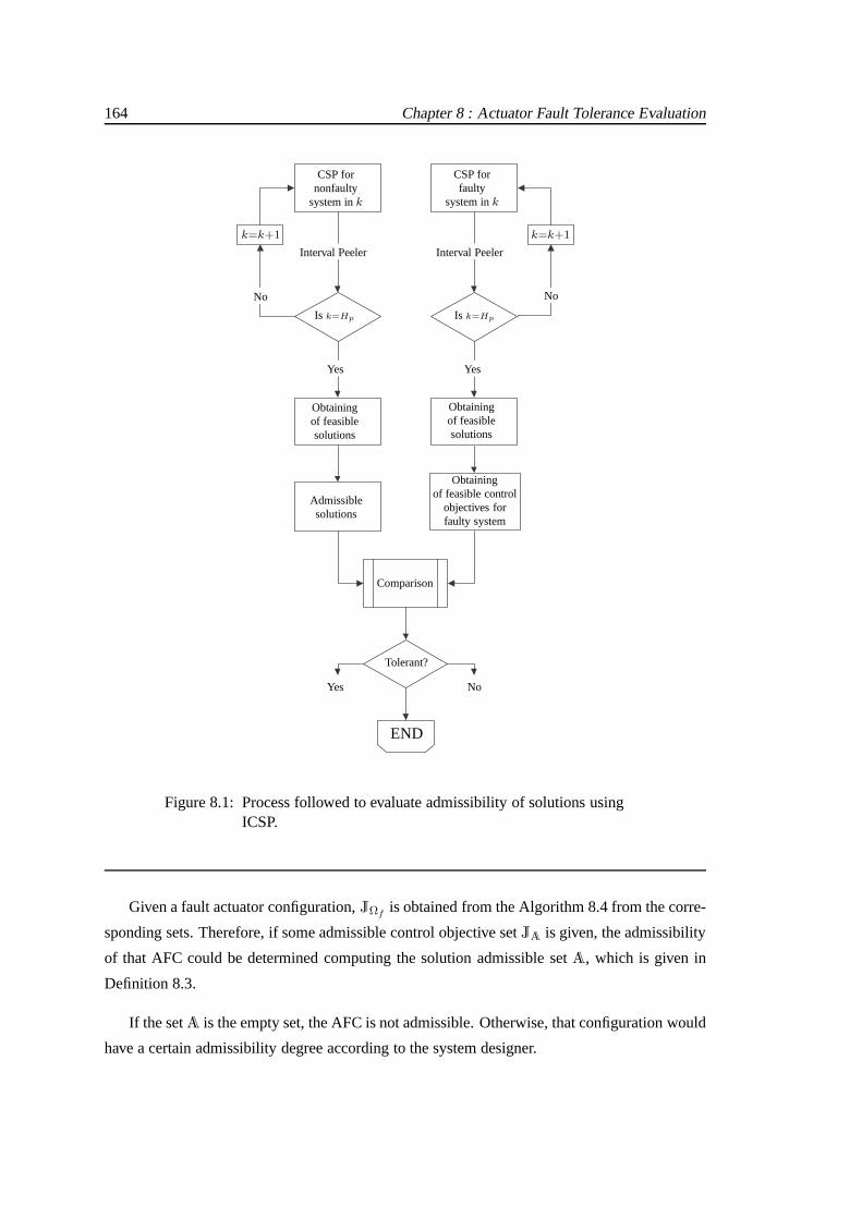
164 Chapter 8 : Actuator Fault Tolerance Evaluation
CSP fornonfaulty
system ink
CSP forfaulty
system ink
k=k+1k=k+1
Interval PeelerInterval Peeler
Is k=HpIs k=Hp
NoNo
No
Comparison
Yes
YesYes
END
Tolerant?
Obtainingof feasiblesolutions
Obtainingof feasiblesolutions
Admissiblesolutions
Obtainingof feasible control
objectives forfaulty system
Figure 8.1: Process followed to evaluate admissibility of solutions usingICSP.
Given a fault actuator configuration,JΩfis obtained from the Algorithm 8.4 from the corre-
sponding sets. Therefore, if some admissible control objective setJA is given, the admissibility
of that AFC could be determined computing the solution admissible setA, which is given in
Definition 8.3.
If the setA is the empty set, the AFC is not admissible. Otherwise, that configuration would
have a certain admissibility degree according to the systemdesigner.

8.3 : Admissibility Evaluation Approaches 165
Algorithm 8.4 Computation ofJΩ usingΩk
1: Xk ⇐ X0
2: Ω0 ⇐ X0
3: for k = 1 toHp do4: ComputeΩk (See Algorithm 8.3)5: ComputeJΩk
usingΩk = Xck ×Uc
k−1
6: end for
7: JΩ =Hp⋃k=0
JΩk
Except in very particular cases, it is not possible to evaluate exactly the three setsXp,
Xc andUc required in Algorithm 8.3. Instead guaranteed outer approximations of these sets,
as accurate as possible, have been proposed and used in the literature. On this way, some
contributions have been done in [OMGVQ] and [OMGPW06], where the problem proposed in
the current chapter is solved using zonotope-based set computations. Another approach to be
used in this way is based on the proposal reported in [OMTP06]and [POMTI06]. There, the
set computations are based on subpavings [JKDW01]. Despitethe particular particular proposal
reported in the latter mentioned papers is used for state estimation, the computational principle
can be applied in the straightforward manner on the admissibility evaluation.
8.3.3 Motivational Example
An example to motivate the usefulness and interest of the proposed method is presented. The
presence of constraints in MPC makes very difficult to proceed with the fault-tolerance analysis
as proposed by [Sta03]. There, the analysis is possible because the expression of how fault
affects the objective function is available using LQR theory. However, in constrained MPC this
expression is not available, although an explicit expression for the controller could be derived
[BMDP02]. This motivates the usefulness of the proposed approach.
Example8.1. The double integrator system proposed by [BMDP02] is considered here, whose
equivalent discrete-time state-space description using the Euler discretization rule is:
xk+1 =
[1 1
0 1
]xk +
[0
1
]uk (8.1)
yk =[
1 0]xk, (8.2)
with the following constraints for states and control signals: x1 ∈ [−15, 15], x2 ∈ [−6, 6] and
u ∈ [−1, 1]. A MPC controller is used to control this system satisfying the associated state and
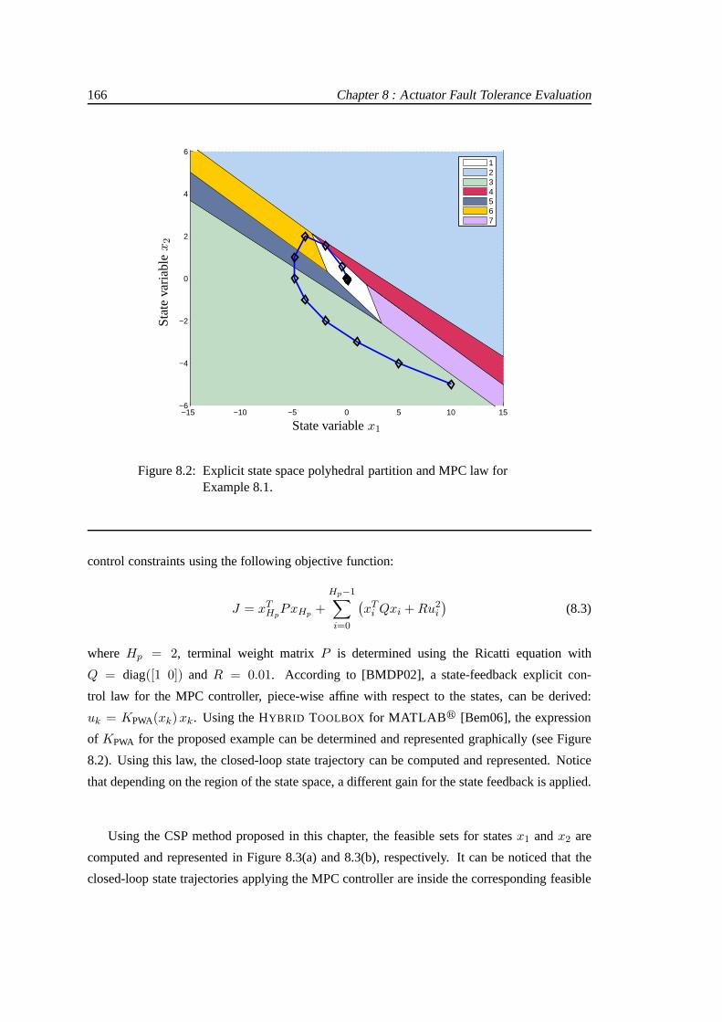
166 Chapter 8 : Actuator Fault Tolerance Evaluation
−15 −10 −5 0 5 10 15−6
−4
−2
0
2
4
61234567
State variablex1
Sta
teva
riabl
ex2
Figure 8.2: Explicit state space polyhedral partition and MPC law forExample 8.1.
control constraints using the following objective function:
J = xTHpPxHp +
Hp−1∑
i=0
(xT
i Qxi +Ru2i
)(8.3)
whereHp = 2, terminal weight matrixP is determined using the Ricatti equation with
Q = diag([1 0]) andR = 0.01. According to [BMDP02], a state-feedback explicit con-
trol law for the MPC controller, piece-wise affine with respect to the states, can be derived:
uk = KPWA(xk)xk. Using the HYBRID TOOLBOX for MATLAB r [Bem06], the expression
of KPWA for the proposed example can be determined and represented graphically (see Figure
8.2). Using this law, the closed-loop state trajectory can be computed and represented. Notice
that depending on the region of the state space, a different gain for the state feedback is applied.
Using the CSP method proposed in this chapter, the feasible sets for statesx1 andx2 are
computed and represented in Figure 8.3(a) and 8.3(b), respectively. It can be noticed that the
closed-loop state trajectories applying the MPC controller are inside the corresponding feasible

8.4 : Actuator Fault Tolerance Evaluation on Sewer Networks 167
sets as expected. Now, a fault in the actuator is introduced.This fault corresponds to a reduction
of the operating range of the actuator such thatu ∈ [−0.75, 0.75]. Computing in this situation
the feasible set for statesx1 andx2 using again the method proposed, it can be noticed that the
closed-loop state trajectories applying the MPC controller in the non-faulty situation are outside
the corresponding feasible sets for the faulty situation. This means that the performance of the
MPC controller will be worse that in the case of the non-faulty actuator since MPC trajectories
for the faulty situation are not reachable. This means that if MPC trajectories in the non-faulty
situation were inside the corresponding feasible sets, theperformance of the MPC controller
would not be affected by the fault, i.e., would be fault-tolerant. This example shows how easily
can be evaluated the tolerance of a control law with respect to a fault using the method proposed.
Moreover, the degradation in the performance can also be evaluated with this method, as it will
be shown in the following application example.
8.4 Actuator Fault Tolerance Evaluation on Sewer Networks
8.4.1 System Description
In order to apply the approach proposed on this chapter for the evaluation of a given AFC within
a sewer network, a small system inspired on the BTC is used. Aswas said before, this 3-tank
catchment (3-TC) contains representative elements of the entire sewer network and considers
three of the four control gates appeared in the BTC. For thesereasons, the 3-TC is enough for
showing the effectiveness of the approach proposed. Hence,the 3-TC, presented in Figure 8.4,
is described by the discrete-time equation in (4.1), where:
A =
1−∆tβ1 0 0
0 1 0
∆tβ1 0 1−∆tβ3
B = ∆t
1 0 0
0 1 −1
−1 −1 1
Bp = ∆t
0 α2 0
0 0 0
1 0 α3
In Figure 8.4,d1 is directly a rain inflow because the virtual tankT1 is not considered
due any gate has influence over its dynamic. Howeverd2k = α2P16k andd4k = α4P20k
are the product of the measurements from the rain-gauges (Pi) and the conversion coefficients
α2 = ϕ2S2 = 0.5951 andα4 = ϕ4 S4 = 0.1530. Parametersβi, ϕi andSi are taken from
Table 3.1 in Chapter 3.
The system constraints expressed in the notation adopted for sewer networks are:

168 Chapter 8 : Actuator Fault Tolerance Evaluation
0 5 10 15 20 25 30 35 40
−15
−10
−5
0
5
10
15
x1
time (s)
(a) Feasible state trajectories forx1.
0 5 10 15 20
−6
−4
−2
0
2
4
6
x2
time (s)
(b) Feasible state trajectories forx2.
Figure 8.3: Feasible set corresponding to the state variables in non-faulty(−) and faulty scenarios (−o−) for Example 8.1. The MPCsolution in a non-faulty situation is also presented (−*−).

8.4 : Actuator Fault Tolerance Evaluation on Sewer Networks 169
T2
T3
T4
qu1
qu2
qu3
R1
q14
q24
q3
qsea
C1
C2
C3
P16
P19
P20
L39
L41
L80
L16
L47
MEDITERRANEAN SEA
EscolaIndustrial
Tank
device
tank
tank
Weir overflow
Level gauge
Redirection
Retention gate
gate
Virtual
Real
rainfall
BesosTreatment
Plant
(WWTP)
Figure 8.4: Application case: Three Tanks Catchment.
• Bounding constraints: refers to physical restrictions.
v2k ∈ [0,+∞] qu1k ∈ [0, 11]
v3k ∈ [0, 35000] qu2k ∈ [0, 25] (8.4)
v4k ∈ [0,+∞] qu3k ∈ [0, 7]

170 Chapter 8 : Actuator Fault Tolerance Evaluation
• Mass conservation constraints
d1k = qu1k + q14k
qx1k = qu2k + q24k (8.5)
qx2k ≥ qu3k
For this application, it is supposed that vectordk (rain) is known at each time instantk ∈ Z+,
what means known perturbation. This causes that the obtained results have only an interest of
design for the tolerant control system.
It is desired to evaluate the admissibility of different AFCnot only in reconfiguration but also
in accommodation. Configuration admissibility is defined from a control objectives degradation
with respect to nominal (without fault) configuration for a given rain episode. The selected rain
corresponds to the one occurred on September 14, 1999, see Figure 3.8(a). This day, severe
flooding occurred as a consequence of the rain storm. The actuator faults are no simultaneous
and they are present from the beginning of the scenario. Their models are described as change
of operating limits (accommodation) or operative annulation (reconfiguration).
Setting-up the Algorithm 8.2
The ICSPH = (Υ,Λ,C) associated to the system has, at each time instantk, the set of variables
with 9 components:
Υ = v2k, v3k, v4k, v2k+1, v3k+1, v4k+1, qu1k, qu2k, qu3k ,
the domains set
Λ = [v2]k, [v3]k, [v4]k, [0,+∞], [0, 35000], [0,+∞], [0, 11], [0, 25], [0, 7]
and the set of constraints given by the corresponding systemmodel 4.1 and expressions in (8.4)
and (8.5).
8.4.2 Control Objective and Admissibility Criterion
The main control objectives are defined as the minimization of the pollution (water volume
that goes to the environment) and the minimization of the CSOto streets (flooding caused by

8.4 : Actuator Fault Tolerance Evaluation on Sewer Networks 171
the insufficient capacity of sewersq14 andq24). Notice that overflows in virtual tanks are not
considered in this case. From system variables, the constraints that defines the control objectives
are given by
• For pollution
J = Venv = ∆t
Hp∑
k=0
max(0, qv4k − q4) (8.6)
• For flooding
J = Vstr = ∆t
Hp∑
k=0
max(0, q14k − q14) + max(0, q24k − q24) (8.7)
Notice that the expression for pollution is expressed in function of a isotone state variable
that has an exact interval hull. Therefore, since pollutiononly depends of this variable, its
interval is also exact as well. In this case,JΩ ⊇ JA holds with equality, what allows an
always correct admissibility evaluation.
On the other hand, when the objective related to flooding is taking into account, its expres-
sion depends of relations between isotone and no isotone variables and therefore, according to
Remark 8.2, the assessment of the non admissible configuration is possible but nothing can be
said about admissibility of the configuration.
The admissibility criterion is based on a direct comparisonbetween the obtained minimum
final value of volume given by the related envelopeV obj(Hp) and the same value for the de-
graded nominal system configurationV nomobj (Hp). Notice that it can be done due to the pollution
and flooding indexes correspond to the accumulated masses over a given scenario). The expres-
sion for the aforementioned comparison is given by
V obj(Hp) = ψ(V nom
obj (Hp))
whereψ is the relation of degradation and subscriptobj denotes the control objective. n order
to illustrate the proposed method, in this application example, it is assumed thatψ = 8. In the
reality, this relation is provided by the network operator according to the directives given by the
city authorities based on the heuristic knowledge of the sewage system designers.

172 Chapter 8 : Actuator Fault Tolerance Evaluation
Table 8.1: Admissibility of AFC for pollution: Reconfiguration.
Fault Location Min. Volume (m3) Admissibility Status
No fault 1050 —Fault inqu1
8800 No AdmissibleFault inqu2
52200 No AdmissibleFault inqu3
1050 Admissible
8.4.3 Obtained Results
Reconfiguration Case
This case considers actuators completely closed or completely open due to the fault. This fact
would change the admissibility of the obtained AFC. Table 8.1 resumes the possible fault cases
and their admissibility when pollution is considered. Onlyfaults described by actuators com-
pletely closed are simulated, that isqui∈ [0, 0] andqi ∈ [0,+∞]. In the contrary case, ICSP
can not be solved due to constraints in ranges ofquiare violated.
On the other hand, Table 8.2 presents the results obtained when flooding is considered.
Notice that some configurations are uncertain due to definition of the cost function for this
objective (see Section 8.4.2).
Table 8.2: Admissibility of AFC for flooding: Reconfiguration.
Fault Location Min. Volume (m3) Admissibility Status
No fault 5100 —Fault inqu1
5100 UncertainFault inqu2
73200 No AdmissibleFault inqu3
5100 Uncertain
Figure 8.5 shows the minimum envelopes for pollution (Figure 8.5(a)) and for flooding
(Figure 8.5(b)) when the admissibility criterion is considered (threshold).
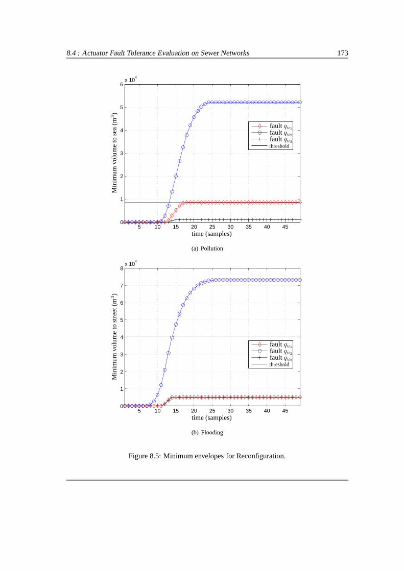
8.4 : Actuator Fault Tolerance Evaluation on Sewer Networks 173
5 10 15 20 25 30 35 40 450
1
2
3
4
5
6x 10
4
time (samples)
Min
imu
mvo
lum
eto
sea
(m3)
fault qu1
fault qu2
fault qu3
threshold
(a) Pollution
5 10 15 20 25 30 35 40 450
1
2
3
4
5
6
7
8x 10
4
time (samples)
Min
imu
mvo
lum
eto
stre
et(m3
)
fault qu1
fault qu2
fault qu3
threshold
(b) Flooding
Figure 8.5: Minimum envelopes for Reconfiguration.

174 Chapter 8 : Actuator Fault Tolerance Evaluation
Accommodation Case
This case considers faults manifested as the reduction of the actuators operative rank (for ex-
ample from 0-100% to 0-50%). Thus, the amount of admitted AFCvaries as it is shown in
Tables 8.3 and 8.4, where if the admissibility criterion is maintained as in the reconfiguration
case, more configurations could be admitted. Different accommodation ranges are presented.
These tables do not consider accommodation forqu3due to the system insensibility shown for
this actuator what is seen in the results collected in Tables8.1 and 8.2. Figure 8.6 presents the
minimum envelopes for pollution and flooding in the case of accommodation.
Table 8.3: Admissibility of fault configurations for pollution:Accommodation.
Fault Location Operation range Min. Volume (m3) Admissibility Status
No fault — 1050 —Fault inqu1
0-20% 5200 AdmissibleFault inqu1
0-50% 2300 AdmissibleFault inqu2
0-20% 34000 No AdmissibleFault inqu2
0-50% 15700 No Admissible
8.5 Summary
This chapter proposes a method for admissibility evaluation of fault configurations based on the
solution of a Interval Constraints Satisfaction Problem (ICSP). This procedure implies the prop-
agation of the feasible solution set at each time instant solving implicitly an interval simulation.
The results provide the limits of system performance considering all the feasible solutions and
how they are degraded after fault occurrence. This allows toevaluate the admissibility of a given
AFC using a degradation criterion established beforehand.
Another techniques could be used for solving the proposed problem of actuator fault toler-
ance evaluation. These techniques are based on set computation using zonotopes, subpavings
and other approximations. However, these techniques are not explained here despite of their
applications have been reported, see [OMGVQ], [OMGPW06], [OMTP06] and [POMTI06].
The proposed method has been successfully applied on a linear predictive control system

8.5 : Summary 175
Table 8.4: Admissibility of fault configurations for flooding:Accommodation.
Fault Location Operation range Min. Volume(m3) Admissibility Status
No fault — 5100 —Fault inqu1
0-20% 5100 UncertainFault inqu1
0-50% 5100 UncertainFault inqu2
0-20% 50000 UncertainFault inqu2
0-50% 26100 No Admissible
inspired on the BTC. This 3-tank catchment (3-TC) contains representative elements of the
entire sewer network and considers three of the four controlgates appeared in the BTC. For
these reasons, the 3-TC is enough for showing the effectiveness of the approach proposed. The
proposed technique on this chapter has been also proved considering a nonlinear model of the
3-TC [OMPQ06]:
v2k+1 = v2k + ∆t [qu1k + d2k − qv2outk]
v3k+1 = v3k + ∆t [qu2k − qu3k]
v4k+1 = v4k + ∆t [qu3k + d3k + q14k + q24k − qv4outk]
(8.8)
where the nonlinear relation between thei-th tank volume vi and the tank outflow
qviout= βi
√vik is considered. Obtained results reported in this referenceshown the ef-
fectiveness of the approach considering the nonlinear model predictive control framework.
On the other hand, in [GOMP07] is proposed the actuator faulttolerance evaluation when
Linear Constrained Robust Model Predictive Control (LRMPC) is used taking into account
model uncertainty. In this case, the problem considers the parameters as new variables to be
refined when the ICSP is stated. Hence, the set of constraintsC for the LRMPC problem is now
defined as:
C :
xk+1 = A(θk)xk +B(θk)uk
xk ∈ X k ∈ [0,Hp] ⊂ Z+
uk ∈ U k ∈ [0,Hp − 1] ⊂ Z+
θk ∈ Θ k ∈ [0,Hp] ⊂ Z+
(8.9)

176 Chapter 8 : Actuator Fault Tolerance Evaluation
5 10 15 20 25 30 35 40 450
0.5
1
1.5
2
2.5
3
3.5x 10
4
time (samples)
Min
imu
mvo
lum
eto
sea
(m3)
fault qu10-20%
fault qu10-50%
fault qu20-20%
fault qu20-50%
threshold
(a) Pollution
5 10 15 20 25 30 35 40 450
0.5
1
1.5
2
2.5
3
3.5
4
4.5
5x 10
4
time (samples)
Min
imu
mvo
lum
eto
stre
et(m3
)
fault qu10-20%
fault qu10-50%
fault qu20-20%
fault qu20-50%
threshold
(b) Flooding
Figure 8.6: Minimum envelopes for Accommodation.

8.5 : Summary 177
where
X∆= x ∈ R
n |x ≤ x ≤ x (8.10a)
U∆= u ∈ R
m |u ≤ u ≤ u (8.10b)
Θ∆=
θ ∈ R
p | θ ≤ θ ≤ θ
(8.10c)
andA(θ) andB(θ) are the system matrices of suitable dimensions including their associated
uncertain parameters. Also the effectiveness of the evaluation approach is proved despite of the
presence of parameter uncertainty.

178 Chapter 8 : Actuator Fault Tolerance Evaluation

Part IV
Concluding Remarks
179


CHAPTER 9
CONCLUDING REMARKS
In conclusion, the thesis objectives has been fulfilled. Furthermore, during the thesis process
new objectives and tasks were appearing. They have enhancedthe proposed approaches and/or
have complemented the obtained results. Therefore, this chapter summarizes the main contri-
butions done and proposes future ways to continue the line ofthe thesis.
9.1 Contributions
The central idea behind this thesis was the design of MPC strategies for sewer networks includ-
ing considerations about fault tolerance. The main contributions of this thesis are summarized
below.
• Lexicographic approach was used as an automatic tuning for the MPC controller of a
sewer network. The application of this technique over such complex systems was moti-
vated by the difficulty of determining the suitable weights for a cost function of a tradi-
tional MPC controller due to the continuous change of the rain intensity (system distur-
bances).
• An hybrid modeling methodology was developed for modeling sewer networks. The
proposed methodology allows to represent each constitutive element of the network as
an hybrid system. To obtain the model of the entire system within this framework, all
preestablished hybrid submodels are joined suitably (taking into account their connections
within the network), avoiding the tedious and complex process of modeling directly the
whole sewer network as an unique hybrid system.
181

182 Chapter 9 : Concluding Remarks
• Predictive control of sewer networks has been proposed by considering their models as
hybrid systems. This fact allows to compute the global optimal solution of the associ-
ated optimization problem despite the sewage system model includes nonlinear dynamics
related to overflows and flood, which implies switching on operating modes.
• A suboptimal HMPC design was derived for reducing the computation time taking by
the solution of the MIP associated to the discrete optimization problem. The obtained
approach guarantees feasibility in the the optimization process and closed-loop stability.
Such suboptimal HMPC design was proved on the sewer network case study, obtaining
satisfactory results related not only with computation time but also with the system sub-
optimality level.
• The hybrid modeling methodology was used to represent actuator faults consisting in
the change of operational ranges of such elements. Also, it was taking into to account
the hybrid nature of the FTC system by using an hybrid systemsmodeling, analysis and
control methodology. This Fact has allowed to design the three levels of a FTC system in
an integrated manner and verify its global behavior.
• A method was described for evaluating the fault tolerance ofa linear MPC closed-loop
under the effect of faults in actuators. Such method uses constraints satisfaction to know
whether a certain configuration of faulty actuators fulfillsthe problem constraints, or
whether the corresponding control objectives are fulfilleddespite the presence of actu-
ator faults. This way of tolerance evaluation avoids solving an optimization problem in
order to know whether the control law can deal with actuator fault configuration.
9.2 Directions for Future Research
To continue the research proposed in this thesis, some ideasare outlined below.
• It would be very useful to derive sewer network models with adaptive parameters which
could be auto-calibrated according to the available information from sensors, statistics
and accurate predictions for rain intensities and their effects over the sewage system.
• The inclusion of inherent switching dynamics in the sewer network model for the MPC de-
sign of Chapter 4 should be further investigated. There exist some inaccurate approaches
for dealing with these nonlinear dynamics1 which can be tested in order to take advantage1for instance, approximations of min or max function by sets of linear inequalities [A.03b].

9.2 : Directions for Future Research 183
of the scalability and self-tuning capabilities without losing the convexity of the optimiza-
tion problem.
• The implementation of a suitable software tool, inspired onthe philosophy of CORAL
[FCP+02], should be done. Such tool would make the automatic integration of the differ-
ent hybrid elements when a given sewer network has been considered as a compositional
hybrid system. The software tool would calculate the globalMLD model related to the
given network.
• The application of tuning methods for MPC controllers basedon Lexicographic program-
ming should be extended to HMPC controllers once suboptimalstrategies have been in-
cluded in the design of such controllers. According to Section 4.2.3, it can be noticed that
if the mentioned tuning methods are considered without taking into account a suboptimal
strategy, the computation time for solving the discrete optimization problem increases
excessively due to the implementation features of the tuning method.
• Within the active approach of the FTHMPC, this thesis assumed that FDI module always
operates correctly. However it can not be ensured for all situations. Even though a false
alarm of fault occurrence (situation when FDI faults) only implies a very conservative
controller2, when FDI does not inform about a fault situation, the activefault tolerant
topology become passive. However, these facts should be investigated with more depth.
• Another important situation that should be investigated isrelated with the existence of
delays in the FDI module and their effects in the performanceof the closed-loop, mainly
by considering the presence of faults. Theoretically, MPC techniques deal with such
problems, however this fact would have to be confirmed when assuming the AFTHMCP
strategy.
• Rain prediction is an active research area which is currently under development and com-
bines different disciplines. This topic is undoubtedly important in the study of sewer
networks and all aspects associated with: modeling, RTC, environmental management,
etc.
Finally, constant changes on the Barcelona sewer network topology in order to improve its
management have produced. Figure 9.1 shows the actual BTC. Considering the new system
topology, it is possible that some of the methodologies, approaches and strategies proposed on
this thesis reach better results than with the older BTC version.2under these conditions, control gates are under-used and this situation is as if the actuators had a self-limiter.

184 Chapter 9 : Concluding Remarks
T1
T2
T3
T4
T5
T6
T7
T8
T9
T10
T11
T12
T13
qu1
qu2
qu3
qu4
qu5
qu6
R1
R2
R3
R4
R5
R6
R7
q14
q24
q96
q96q910
qc210 q945
q946
q10M
q10D
q57
q68
q7M
q128
q12sq811
q8M
q11B
q11M
q7L
C1
C2
C3
CR
CR
P13
P14
P16
P16
P16
P19
P20
P20
P20
P20
P20
L39
L41
L80
L80
L16
L53
L53
L53
L9
L27
L
L
L
L
L
L3
L11
L47
L56
L7
L8
L8
MEDITERRANEAN
SEA
EscolaIndustrial
Tank
Overflowelement
tank
tankVirtual
Real
Rain-gauge
Level gauge
Redirection
Retention gate
gate
(WWTP 1)LlobregatTreatment
Plant
(WWTP 2)Besos
TreatmentPlant
Figure 9.1: New topology for the BTC.

Part V
Appendices
185


APPENDIX A
PROOF OFTHEOREM 6.1
Consider the shifted sequence
u1k+1 ,
(u∗1|k, . . . , u
∗Hp−1|k, h(xHp−1|k+1)
)(A.1)
wherexHp−1|k+1 is the state at prediction timeHp − 1, obtained at timek + 1 by applying
the input sequenceu∗1|k, . . . , u∗Hp−1|k to system (6.4) with initial conditionx0|k+1 , x∗1|k =
xk+1 = g(xk, uMPC(xk)). Note thatxHp−1|k+1 = x∗Hp|k.
1. If Problem 6.1 is feasible at timek ∈ Z+ for statexk ∈ X then there exists a mode se-
quence reference∆k such thatU(xk, ∆k) is nonempty. The optimal solution to Problem
6.1 is denotedu∗k. Then it follows thatxHp−1|k+1 ∈ XT . Due to Remark 6.2 and the pos-
itive invariance ofXT ∈ XU, it holds thatxHp|k+1 ∈ XT andu1k+1 ∈ U(xk+1, ∆k+1).
This implies that Problem 6.1 is feasible at timek + 1 for xk+1 and mode sequence
reference∆k+1.
2. Let x(xk) = (x1|k, x2|k . . . xHp|k) denote the state sequence generated by the system
xk+1 = g(xk, h(xk)) from initial statex0|k , xk ∈ XT . Let uk denote the corresponding
control signal. Sincexk ∈ XHp
T , thenuk ∈ U according to Assumption 6.1. A candidate
reference sequence∆k so thatUk(xk, ∆k) is nonempty is the one related touk andxk.
3. Consider again the state sequencexk(xk). Sincexk(xk) ∈ XHp
T , inequality (6.12c) from
187

188 Appendix A : Proof of Theorem 6.1
Remark 6.2 holds for all elements in the sequencexk, yielding
F (x1|k)− F (x0|k) + L(x0|k, h(x0|k)) ≤0
F (x2|k)− F (x1|k) + L(x1|k, h(x1|k)) ≤0
...
F (xHp|k)− F (xHp−1|k) + L(xHp−1|k, h(xHp−1|k)) ≤0.
From these inequalities, by optimality and by Remark 6.2 it follows that
VMPC(xk) ≤ J(xk, uk) ≤ F (xk) ≤ α2(‖xk‖), ∀xk ∈ N
whereN = N ∩XT . Again, using optimality, one has:
VMPC(xk+1)− VMPC(xk) = J(xk+1,u∗k+1)− J(xk,u
∗k)
≤ J(xk+1,u1k+1)− J(xk,u
∗k)
= −L(xk, uMPC(xk)) + F (xHp|k+1)− F (x∗Hp|k)
+ L(x∗Hp|k, h(x∗Hp |k
)).
Then, asx∗Hp|k∈ XT and by condition (6.12c) in Assumption 6.1, it holds that
VMPC(g(xk, uMPC(xk))) − VMPC(xk) ≤ −L(xk, uMPC(xk)) ≤ −α1(‖xk‖) ∀xk ∈ Xf (Hp).
SinceX is compact andXf ⊂ X, then according to item 1.,Xf (Hp) is positively invari-
ant. Letxk be a state reached with the closed-loop system (6.4) and (6.10) from initial
statex0. Chose anyη > 0 such that the ballBη , x ∈ Rn|‖x‖ ≤ η satisfiesBη ⊂ N .
It is possible to chose any0 < ǫ ≤ η a σ ∈ (0, ǫ) such thatα(σ) < α(ǫ). For any
x0 ∈ Bσ ⊂ Xf (Hp), due to positive invariance ofXf (Hp), it follows that
... ≤ VMPC(xk+1) ≤ VMPC(xk+1) ≤ · · · ≤ VMPC(x0) ≤ α2(‖x0‖) ≤ α2(σ) ≤ α1(ǫ).
Since we haveVMPC(x) ≥ α1(ǫ) for all x ∈ Xf (Hp)\Bǫ it follows thatxk ∈ Bǫ for all
k ∈ Z+.

APPENDIX B
AUXILIARY DATA FOR CHAPTER 5
Table B.1: Relation betweenz variables and control objectives.
Objective zvector zvariable Description
z2 overflow inT1
z6 overflow inT2
z10 overflow inT4
z12 overflow inT9
z20 overflow inT5
1 zstrv z22 overflow inT6
z24 overflow inT7
z26 overflow inT12
z32 overflow inT8
z36 overflow inT10
z40 overflow inT11
z4 overflow inq14z8 overflow inq24
2 zstrq z14 overflow inq96z18 overflow inq945z30 overflow inq12s
z34 overflow inqc210
z29 flow to environment (q12s)z35 flow to sea (q10M)
3 zsea z38 flow to sea (q8M)z42 flow to sea (q11M)z44 flow to sea (q7M)
4 — z43 flow to Llobregat WWTP— z41 flow to Besos WWTP
189

190 Appendix B : Auxiliary Data for Chapter 5

APPENDIX C
ACRONYMS
AFC Actuator Fault Configuration
AFTHMPC Active Fault Tolerant Hybrid Model Predictive Control
AFTMPC Active Fault Tolerant Model Predictive Control
AKF Adaptive Kalman Filter
AS Automatic Supervisor
BTC Barcelona Test Catchment
CLABSA Clavegueram de Barcelona, S.A.
CSO Combined Sewage Overflow
CSP Constraint Satisfactions Problem
CSS Combined Sewage System
DEDS Discrete-Event Dynamical System
FDI Fault Diagnosis and Isolation
FTC Fault Tolerant Control
FTHMPC Fault Tolerant Hybrid Model Predictive Control
GPC Global Predictive Control
HMPC Hybrid Model Predictive Control
HYSDEL HYbrid System DEscription Language
ICSP Interval Constraints Satisfaction Problem
LC Linear Complementarity
LCMPC Linear Constraint Model Predictive Control
LP Linear Program(ming)
LPV Linear Parameter Variant
LQR Linear Quadratic Regulator
191

192 Appendix C : Acronyms
LCRMPC Linear Constrained Robust Model Predictive Control
LTI Linear Time Invariant
MBPC Model-Based Predictive Control
MILP Mixed Integer Linear Program(ming)
MIMO Multi-Input Multi-Output
MIP Mixed Integer Program(ming)
MIQP Mixed Integer Quadratic Program(ming)
MLD Mixed Logical Dynamics
MMPS Min-Max-Plus Scaling
MPC Model Predictive Control
NMPC Nonlinear Model Predictive Control
mpLP Multi-Parametric Linear Program(ming)
mpQP Multi-parametric Quadratic Program(ming)
NLP Nonlinear Programming Algorithms
OOP Open-loop Optimization Problem
PFTHMPC Passive Fault Tolerant Hybrid Model Predictive Control
PFTMPC Passive Fault Tolerant Model Predictive Control
PWA Piecewise Affine
QP Quadratic Program(ming)
RLS Recursive Least-Squares
RTC Real-Time Control
SCADA Supervisory Control and Data Acquisition
VFC Volume/Flow Conversion

BIBLIOGRAPHY
[A.03a] ILOG S. A. ILOG CPLEX 9.0 Parameters, October 2003.
[A.03b] ILOG S. A. ILOG CPLEX 9.1 User´s Manual, 2003.
[ABC05] T. Alamo, J.M. Bravo, and E.F. Camacho. Guaranteed state estimation by zono-
topes.Automatica, 41(6):1035–1043, 2005.
[AGBG06] M. Abdel-Geliel, E. Badreddin, and A. Gambier. Application of model predictive
control for fault tolerant system using dynamic safety margin. In Proceedings of
the IEEE American Control Conference, December 2006.
[AHS01] S. Attouche, S. Hayat, and M Staroswiecki. An efficient algorithm for the design
of fault tolerant multi-sensor system. InProceedings of the IEEE Conference on
Decision and Control, volume 2, pages 1891–1892, 2001.
[AS03] D. Angeli and E.D. Sontag. Monotone control systems.IEEE Trans. Automatic
Control, 48(10):1684–1698, October 2003.
[AS05] A. Ames and S. Sastry. Characterization of zeno behavior in hybrid systems
using homological methods. InProceedings of the IEEE American Control Con-
ference, pages 1160–1165, Portland, OR, USA, June 2005.
[Bag05] X. Baguenard. Personal homepage. http://www.istia.univ-angers.fr/∼baguenar/,
February 2005.
[BBBM05] F. Borrelli, M. Baotic, A. Bemporad, and M. Morari. Dynamic programming for
constrained optimal control of discrete-time linear hybrid systems.Automatica,
41:1709–1721, 2005.
[BBM98] M. S. Branicky, V. S. Borkar, and S. K. Mitter. A unified framework for hybrid
control: Model and optimal control theory.IEEE Transactions on Automatic
Control, 43(1):31–45, 1998.
193

194 BIBLIOGRAPHY
[BBM02] A. Bemporad, F. Borrelli, and M. Morari.Hybrid Systems: Computation and
Control, volume 228 ofLecture Notes of Computer Science, chapter On the opti-
mal control law for linear discrete time hybrid systems, pages 105–119. Springer,
Berlin, 2002.
[Bem04] A. Bemporad. Efficient conversion of mixed logical dynamical systems into an
equivalent piecewise affine form.IEEE Trans. Automatic Control, 49(5):832–
838, 2004.
[Bem06] A. Bemporad.Hybrid Toolbox - User’s Guide, April 2006.
[BFG+00] R. Bixby, M. Fenelon, Z. Gu, E. Rothberg, and R. Wunderling. Mip: Theory and
practice – closing the gap. In M. J. D. Powell and S. Scholtes,editors,System
Modelling and Optimization: Methods, Theory and Applications, pages 19–49.
Kluwer Academic Publishers, 2000.
[BG06] A. Bemporad and N. Giorgetti. Logic-based solution methods for optimal control
of hybrid systems. IEEE Transactions of Automatic Control, 51(6):963–976,
June 2006.
[Bix02] R. Bixby. Solving real-world linear programs: a decade and more of progress.
Operations Research, 50(1):3–15, 2002.
[BKB+05] F. Borrelli, T. Keviczky, G. J. Balas, G. Stewart, K. Fregene, and D. Godbole. Hy-
brid decentralized control of large scale systems. In M. Morari and L. Thiele, ed-
itors,Hybrid Systems: Computation and Control, volume 3414 ofLecture Notes
of Computer Science, pages 168–183. Springer Verlag, March 2005.
[BKLS03] M. Blanke, M. Kinnaert, J. Lunze, and M. Staroswiecki. Diagnosis and Fault-
Tolerant Control. Springer-Verlag Berlin Heidelberg, 2003.
[Bla99] M. Blanke. Fault-tolerant control systems. InNew Trends in Advanced Control.
Springer-Verlag, 1999.
[Bla01] M. Blanke. Concepts and methods in fault-tolerant control. Proceedings of the
IEEE American Control Conference, 4:2606–2620, 2001.
[BM99a] A. Bemporad and M. Morari. Control of systems integrating logic, dynamics,
and constraints.Automatica, 35(3):407–427, 1999.

BIBLIOGRAPHY 195
[BM99b] A. Bemporad and M. Morari. Robust model predictive control: A survey. In
A. Garulli, A. Tesi, and A. Vicino, editors,Robustness in Identification and Con-
trol, number 245, pages 207–226. Springer-Verlag, 1999.
[BMDP02] A. Bemporad, M. Morari, V. Dua, and E. Pistikopoulos. The explicit linear
quadratic regulator for constrained systems.Automatica, 38(1):3–20, 2002.
[Bor00] C. Bordons. Control predictivo: metodologıa, tecnologıa y nuevas perspecti-
vas. Technical report, Departamento de Ingenierıa de Sistemas y Automatica,
Universidad de Sevilla, Aguadulce, Almerıa, 2000.
[BPD99] S.M. Bennett, R.J. Patton, and S. Daley. Sensor fault-tolerant control of a rail
traction drive.Control Engineering Practice, 7:217–225, 1999.
[Bra04] J.M. Bravo.Control predictivo no lineal robusto basado en tecnicas intervalares.
PhD thesis, Escuela Supeior de Ingenieros, Universidad de Sevilla, Espana, Junio
2004.
[BSS06] M. Bazaraa, H. Sherali, and C. Shetty.Nonlinear Programming: Theory and
Algorithms. John Wiley and Sons Ltd., 3rd edition, June 2006.
[BT00] V. Blondel and J.N. Tsitsiklis. A survey of computational complexity results in
systems and control.Automatica, 36:1249–1274, 2000.
[BU94] M. Brdys and B. Ulanicki.Operational Control of Water Systems: Structures,
algorithms and applications. Prentice Hall International, 1994.
[BV04] S. Boyd and L. Vandenberghe.Convex Optimization. Cambridge University
Press, 2004.
[BZ00] M.S. Branicky and G. Zhang. Solving hybrid control problems: Level sets and
behavioral programming. InProceedings of the IEEE American Control Confer-
ence, June 2000.
[CB04] E.F. Camacho and C. Bordons.Model Predictive Control. Springer-Verlag, Lon-
don, second edition, 2004.
[CLA05] Clavegueram de Barcelona S.A. CLABSA. Homepage. http://www.clabsa.es/,
2005.

196 BIBLIOGRAPHY
[CLO95] C.G. Cassandras, S. Lafortune, and G.J. Olsder. Introduction to the modelling,
control and optimisation of discrete event systems. In A. Isidori, editor,Trends
in Control. Springer-Verlag, 1995.
[CPC98] J. Chen, R.J. Patton, and Z. Chen. An LMI approach to fault-tolerant control
of uncertain systems. InProceedings of the IEEE Conference on Decision and
Control, volume 1, pages 175–180, 1998.
[CPSE02] P. Cuguero, V. Puig, J. Saludes, and T. Escobet. A class of uncertain linear
interval models for which a set based robust simulation can be reduced to few
pointwise simulations. InProceedings of the IEEE Conference on Decision and
Control, volume 2, pages 1862–1863, 2002.
[CQ99] G. Cembrano and J. Quevedo.Optimization in water networks. Research Studies
Press, 1999.
[CQS+04] G. Cembrano, J. Quevedo, M. Salamero, V. Puig, J. Figueras, and J. Martı. Opti-
mal control of urban drainage systems: a case study.Control Engineering Prac-
tice, 12(1):1–9, 2004.
[Cro05] A. Crossley. Accurate and efficient numerical solutions for the Saint-Venant
equations of open channel flow. PhD thesis, Faculty of Engineering, School of
Civil Engineering, University of Nottingham, 2005.
[DMDV01] S. Duchesne, A. Mailhot, E. Dequidt, and J. Villeneuve. Mathematical modeling
of sewers under surcharge for real time control of combined sewer overflows.
Urban Water, 3:241–252, 2001.
[DMHN99] V. Dardinier-Maron, F. Hamelin, and H. Noura. A fault-tolerant control design
against major actuator failures: application to a three-tank system. InProceed-
ings of the IEEE Conference on Decision and Control, volume 4, pages 3569–
3574, 1999.
[DMV04] S. Duchesne, A. Mailhot, and J. Villeneuve. Global predictive real-time control
of sewers allowing surcharged flows.Journal of Environmental Engineering,
130(5):526–534, 2004.
[DP01] Y. Diao and K.M. Passino. Stable fault-tolerant adaptive fuzzy/neural control for
a turbine engine.IEEE Trans. Control Syst. Techn., 9:494–509, 2001.

BIBLIOGRAPHY 197
[DP02] Y. Diao and K.M. Passino. Intelligent fault-tolerant control using adaptive and
learning methods.Control Engineering Practice, 10:494–509, 2002.
[EC01] L. ElGhaoui and G. Calafiore. Robust filtering for discrete-time systems with
bounded noise and parametric uncertainty.IEEE Trans. Automatic Control,
46(7):1084–1089, 2001.
[ED05] M.G. Earl and R. D’Andrea. Phase transitions in the multi-vehicle task assign-
ment problem. InProceedings of IMECE2005 2005 ASME International Me-
chanical Engineering Congress and Exposition, 2005.
[EP04] D.W. Etherington and A.J. Parkes. Improving coalition performance by exploit-
ing phase transition behavior. Technical report, Computational Intelligence Re-
search Laboratory, 1269 University of Oregon, June 2004. DARPA Autonomous
Negotiating Teams (ANTs) Project.
[Erm99] Y. Ermolin. Mathematical modelling for optimized control of Moscow’s sewer
network.Applied Mathematical Modelling, 23:543–556, 1999.
[FCP+02] J. Figueras, G. Cembrano, V. Puig, J. Quevedo, M. Salamero, and J. Martı. Coral
off-line: an object-oriented tool for optimal control of sewer networks. InPro-
ceedings on IEEE International Symposium on computer aidedcontrol system
design, volume 1, pages 224–229, 2002.
[FP01] C. Floudas and P. Pardalos. Encyclopedia of optimization. Kluwer Academic
Publishers, 2001.
[Gey05] T. Geyer.Low Complexity Model Predictive Control in Power Electronics and
Power Systems. PhD thesis, March 2005.
[GOMP07] P. Guerra, C. Ocampo-Martınez, and V. Puig. Actuator fault tolerance evaluation
of linear constrained robust model predictive control. InProceedings of the IEEE
European Control Conference, 2007. Accepted for publication.
[GR94] M. Gelormino and N. Ricker. Model-predictive control of a combined sewer
system.International Journal of Control, 59:793–816, 1994.
[GRA07] Group of Applied Research on Hydrometeorology GRAHI. Homepage.
http://www.grahi.upc.es/, 2007.

198 BIBLIOGRAPHY
[GSdD05] G. Goodwin, M. Seron, and J. de Dona.Constrained Control and Estimation:
An optimisation approach. Springer-Verlag, 2005.
[GTM03] T. Geyer, F.D. Torrisi, and M. Morari. Efficient ModeEnumeration of Compo-
sitional Hybrid Models.Hybrid Systems: Computation and Control, 2623:216–
232, April 2003.
[GW94] I.P. Gent and T. Walsh. The SAT phase transition. In A.Cohn, editor,Proceed-
ings of 11th European Conference on Artifitial Intelligence. John Wiley & Sons,
Ltd., 1994.
[HDB01] W.P.M.H. Heemels, B. De Schutter, and A. Bemporad. Equivalence of hybrid
dynamical models.Automatica, 37:1085–1091, 2001.
[HIM01] Y. Huo, P. Ioannou, and M. Mirmirani. Fault-tolerant control and reconfiguration
for high performance aircraft: Review. Technical Report 01-11-01, University of
Southern California Deptartament of Electrical Engineering-Systems, Los An-
geles, CA 90089 California State University, Los Angeles Dept. of Mechanical
Engineering, 2001.
[HLMR02] M. Heymann, F. Lin, G. Meyer, and S. Resmerita. Analysis of zeno behaviors
in hybrid systems. Technical report, Technion - Computer Science Department,
March 2002.
[HSA00] G. Hoblos, M. Staroswiecki, and A. Aitouche. Optimal design of fault tolerant
sensor networks. InProceedings of IEEE International Conference on Control
Applications, volume 1, pages 467–472, 2000.
[Hyv92] E. Hyvonen. Constraint reasoning based on interval arithmetic: The tolerance
approach.Artificial Intelligence, 58:71–112, 1992.
[IS95] K. Ikeda and S. Shin. Fault tolerant decentralized adaptive control systems using
backstepping. InProceedings of the IEEE Conference on Decision and Control,
volume 3, pages 2340–2345, 1995.
[Jia94] J. Jiang. Design of reconfigurable control systems using eigenstructure assign-
ment. International Journal of Control, 59:395–410, 1994.
[JKBW01] L. Jaulin, M. Kieffer, I. Braems, and E. Walter. Guaranteed nonlinear esti-
mation using constraint propagation on sets.International Journal of Control,
74(18):1772–1782, 2001.

BIBLIOGRAPHY 199
[JKDW01] L. Jaulin, M. Kieffer, O. Didrit, and E. Walter.Applied Interval Analysis, with
Examples in Parameter and State Estimation, Robust Controland Robotics.
Springer-Verlag, London, 2001.
[Joh00] K.H. Johansson. Hybrid systems: modeling, analysis and control - open hybrid
automata and composition. Lecture notes of the class EECS 291e, Lecture 5,
University of California at Berkley, 2000.
[KBM +00] E.C. Kerrigan, A. Bemporad, D. Mignone, M. Morari, and J.M. Maciejowski.
Multi-objective prioritisation and reconfiguration for the control of constrained
hybrid systems. InProceedings of the American Control Conference, pages
1694–1698, Chicago, IL, 2000.
[Kuh98] W. Kuhn. Rigorously computed orbits of dynamicalsystems without the wrap-
ping effect.Computing, 61(1):47–67, 1998.
[KJW02] M. Kieffer, L. Jaulin, and E. Walter. Guaranteed recursive non-linear state bound-
ing using interval analysis.International Journal of Adaptive Control and Signal
Processing, 16(3):193–218, 2002.
[KM02] E. Kerrigan and J. Maciejowski. Designing model predictive controllers with pri-
oritised constraints and objectives. InProceedings of IEEE International Sympo-
sium on Computer Aided Control System Design, volume 1, pages 33–38, 2002.
[Kun92] C. Kung. Optimal model matching control for mimo continuous-time systems.
In Proceedings of Singapore International Conference on Intelligent Control and
Instrumentation, volume 1, pages 42–47, 1992.
[Laz06] M. Lazar.Model Predictive Control of Hybrid Systems: Stability and Robustness.
PhD thesis, Technische Universiteit Eindhoven, 2006.
[LDC99] S. Lyshevski, K. Dunipace, and R. Colgren. Identification and reconfigurable
control of multivariable aircraft. InProceedings of the IEEE American Control
Conference, volume 4, pages 2732–2736, 1999.
[LHWB06] M. Lazar, W.P.M.H. Heemels, S. Weiland, and A. Bemporad. Stability of hybrid
model predictive control.IEEE Transactions of Automatic Control, 51(11):1813
– 1818, 2006.
[Lju99] L. Ljung. System Identification—Theory for the User, Second Edition. Prentice
Hall, 1999.

200 BIBLIOGRAPHY
[LLL00] Y. Liang, D. Liaw, and T. Lee. Reliable control of nonlinear systems. 45:706–
710, 2000.
[LP04] F. Lydoire and P. Poignet. Commande non lineaire a horizon fuyant
via l’arithmetique d’intervalles. Conference Internationale Francophone
d’Automatique, (66), 2004.
[LR01] B. Lincoln and A. Rantzer. Optimizing linear system switching. InProceedings
of the 40th IEEE conference on Decision and Control, pages 2063–2068, 2001.
[LS03] J. Lunze and T. Steffen. Control reconfiguration by means of a virtual actuator.
In Proceedings of IFAC SAFEPROCESS, pages 133–138, 2003.
[LTS99] J. Lygeros, C. Tomlin, and S. Sastry. Controllers for reachability specifications
for hybrid systems.Automatica, 35(3):349 – 370, 1999.
[LWY02] F. Liao, J. Wang, and G. Yang. Reliable robust flight tracking control: an lmi
approach.IEEE Trans. Control Syst. Techn., 10:76–89, 2002.
[Mac97] J.M. Maciejowski. Reconfiguring control systems byoptimization. InProceed-
ings of the European Control Conference, Brussels, July 1997.
[Mac98] J.M. Maciejowski. The implicit daisy-chaining property of constrained predic-
tive control.Applied Mathematics and Computer Science, 8:695–711, 1998.
[Mac99] J.M. Maciejowski. Fault-tolerant aspects of MPC. In Procedings of IEE Work-
shop on Model Predictive Control: Techniques and Applications, 1999.
[Mac02] J.M. Maciejowski. Predictive Control with Constraints. Prentice Hall, Great
Britain, 2002.
[Mar99] M. Marinaki. A non-linear optimal control approachto central sewer network
flow control. International Journal of Control, 72(5):418–429, March 1999.
[May04] L.W. Mays.Urban Stormwater Management Tools. McGrawHill, 2004.
[MBB03] M. Morari, M. Baotic, and F. Borrelli. Hybrid systems modeling and control.
European Journal of Control, 9:177–189, 2003.
[Mie99] K.M. Miettinen. Non-linear Multiobjective Optimization. Kluwer Academic
Publishers, 1999.

BIBLIOGRAPHY 201
[MJ03] J.M. Maciejowski and C.N. Jones. MPC fault-tolerantflight control case study:
Flight 1862. InIFAC Safeprocess Conference, Washington DC, June 2003.
[ML01] J.M. Maciejowski and J.M. Lemos. Predictive methodsfor ftc. In K.J Astrom,
P. Albertos, M. Blanke, A. Isidori, W. Schaufelberger, and R. Sanz, editors,Con-
trol of Complex Systems, pages 229–240. Springer-Verlag, 2001.
[MMM01] V.G. Mitchell, R.G. Mein, and T.A. McMahon. Modelling the urban water cycle.
Environmental Modelling & Software, 16:615 – 629, 2001.
[MP97] M. Marinaki and M. Papageorgiou. Central flow controlin sewer networks.
Journal of Water Resources, Planning and Management, 123(5):274 – 283, 1997.
[MP98] M. Marinaki and M. Papageorgiou. Nonlinear optimal flow control for sewer
networks. InProceedings of the IEEE American Control Conference, volume 2,
pages 1289–1293, 1998.
[MP01] M. Marinaki and M. Papageorgiou. Rolling-horizon optimal control of sewer
networks. InProceedings of the IEEE International Conference on Control Ap-
plications, volume 1, pages 594–599, 2001.
[MP05] M. Marinaki and M. Papageorgiou.Optimal Real-time Control of Sewer Net-
works. Springer, 2005.
[MR93] J.M. Maciejowski and W.F. Ramirez. Controlling systems in the face of faults.
In Proceedings of the IEEE Colloquium on Fault Diagnosis and Control System
Reconfiguration, 1993.
[MRRS00] D. Mayne, J.B. Rawlings, C.V. Rao, and P.O.M. Scokaert. Constrained model
predictive control: Stability and optimality.Automatica, 36:789–814, 2000.
[MVSdC06] L.F. Mendonca, S.M. Vieira, J.M.C. Sousa, and J.M.G. Sa da Costa. Fault ac-
commodation using fuzzy predictive control. InProceedings of the IEEE Inter-
national Conference on Fuzzy Systems, 2006.
[MZK +99] R. Monasson, R. Zecchina, S. Kirkpatrick, B. Selman, andL. Troyansky. De-
termining computational complexity from characteristic “phase transitions”.Na-
ture, 400:133–137, July 1999.
[Neu93] A. Neumaier. The wrapping effect, ellipsoid arithmetic, stability and confidence
regions.Computing Supplementum, 9:175–190, 1993.

202 BIBLIOGRAPHY
[NLBH+04] E. Nudelman, K. Leyton-Brown, H. H. Hoos, A. Devkar, and Y. Shoham. Un-
derstanding random SAT: Beyond the classes-to-variables ratio. InProceedings
of the Tenth International Conference on Principles and Practice of Constraint
Programming, volume 3258 ofLecture Notes in Computer Science, pages 438–
452, Toronto, Canada, 2004. Springer.
[OM04] C. Ocampo-Martinez. Benchmark definition for fault tolerant control based on
Barcelona sewer network. Internal report, Universidad Politecnica de Catalunya
(UPC) -ESAII, May 2004.
[OM05] C. Ocampo-Martinez. Barcelona sewer network problem: Model based on piece-
wise functions. Technical report, Technical University ofCatalonia (UPC) -
ESAII, July 2005.
[OMGPW06] C. Ocampo-Martınez, P. Guerra, V. Puig, and M. Witczak. Actuator fault toler-
ance evaluation of linear constrained MPC. InProceedings of the 4th Workshop
on Advanced Control and Diagnosis, Nancy, France, November 2006. Universite
Henri Poincare de Nancy.
[OMGVQ] C. Ocampo-Martınez, P. Guerra, V.Puig, and J. Quevedo. Actuator fault tolerance
evaluation of linear constrained MPC using zonotope-basedset computations.
Submitted to Journal of Systems & Control Engineering, 2007.
[OMIPQ06] C. Ocampo-Martınez, A. Ingimundarson, V. Puig,and J. Quevedo. Hybrid model
predictive control applied on sewer networks: The Barcelona case study. In
F. Lamnabhi-Lagarrigue, S. Laghrouche, A. Loria, and E. Panteley, editors,Tam-
ing Heterogeneity and Complexity of Embedded Control (CTS-HYCON Work-
shop on Nonlinear and Hybrid Control). International Scientific & Technical
Encyclopedia (ISTE), 2006.
[OMPQ06] C. Ocampo-Martınez, V. Puig, and J. Quevedo. Actuator fault tolerance evalua-
tion of constrained nonlinear MPC using constraints satisfaction. InProceedings
of IFAC SAFEPROCESS, Beijing (China), 2006.
[OMPQI05] C. Ocampo-Martinez, V. Puig, J. Quevedo, and A. Ingimundarson. Fault tolerant
model predictive control applied on the Barcelona sewer network. In Proceed-
ings of IEEE Conference on Decision and Control (CDC) and European Control
Conference (ECC), 2005.

BIBLIOGRAPHY 203
[OMTP06] C. Ocampo-Martınez, S. Tornil, and V. Puig. Robust fault detection using inter-
val constraints satisfaction and set computations. InProceedings of IFAC SAFE-
PROCESS, Beijing (China), 2006.
[Pap85] M. Papageorgiou. Optimal multireservoir network control by the discrete maxi-
mum principle.Water Resour. Res., 21(12):1824 – 1830, 1985.
[Pap94] C. Papadimitriou.Computational Complexity. Addison-Wesley, 1994.
[Pat97] R.J. Patton. Fault-tolerant control: the 1997 situation. InProceedings of IFAC
SAFEPROCESS, pages 1033–1055, 1997.
[PCL+05] M. Pleau, H. Colas, P. Lavallee, G. Pelletier, and R. Bonin. Global optimal real-
time control of the Quebec urban drainage system.Environmental Modelling &
Software, 20:401–413, 2005.
[PLM99] F. Previdi, M. Lovera, and S. Mambretti. Identification of the rainfall-runoff
relationship in urban drainage networks.Control Engineering Practice, 7:1489–
1504, 1999.
[PMLC96] M. Pleau, F. Methot, A. Lebrun, and A. Colas. Minimizing combined sewer
overflow in real-time control applications.Water Quality Research Journal of
Canada, 31(4):775 – 786, 1996.
[PMNS06] S.C. Patwardhan, S. Manuja, S. Narasimhan, and S.L. Shah. From data to di-
agnosis and control using generalized orthonormal basis filters. Part II: Model
predictive and fault tolerant control.Journal of Process Control, 16:157 – 175,
2006.
[PNP05] J. Prakash, S. Narasimhan, and S. Patwardhan. Integrating model based fault
diagnosis with model predictive control.Industrial and engineering chemistry
research, 44:4344 – 4360, 2005.
[POMTI06] V. Puig, C. Ocampo-Martınez, S. Tornil, and A. Ingimundarson. Robust fault de-
tection using set-membership estimation and constraints satisfaction. InProceed-
ings of the International Workshop on Principles of Diagnosis DX, Valladolid
(Spain), June 2006.
[PPC+01] M. Pleau, G. Pelletier, H. Colas, P. Lavallee, and R. Bonin. Global predictive
real-time control of Quebec Urban Community’s Westerly sewer network.Water
Science Technology, 43(7):123–130, 2001.

204 BIBLIOGRAPHY
[PSN+04] B.T. Polyak, S.A. Sergey, A. Nazin, C. Durieu, and E. Walter. Ellipsoidal param-
eter or state estimation under model uncertainty.Automatica, 40(7):1171–1179,
2004.
[PSQ03] V. Puig, J. Saludes, and J. Quevedo. Worst-case simulation of discrete linear
time-invariant interval dynamic systems.Reliable Computing, 9(4):251–290,
2003.
[QGP+05] J. Quevedo, G.Cembrano, V. Puig, R.and J. Figueras, and R. Gustavo. First
results of predictive control application on water supply and distribution in
Santiago-Chile. In16th IFAC World Congress, 2005.
[QIYS01] Z. Qu, C.M. Ihlefeld, J. Yufang, and A. Saengdeejing. Robust control of a class
of nonlinear uncertain systems. fault tolerance against sensor failures and sub-
sequent self recovery. InProceedings of the IEEE Conference on Decision and
Control, volume 2, pages 1472–1478, 2001.
[QIYS03] Z. Qu, C.M. Ihlefeld, J. Yufang, and A. Saengdeejing. Robust fault-tolerant self-
recovering control of nonlinear uncertain systems.Automatica, 39:1763–1771,
2003.
[RL95] N.L. Ricker and J.H. Lee. Nonlinear model predictivecontrol of the tennessee
eastman challenge process.Computers & Chemical Engineering, 19(9):961 –
981, 1995.
[SA00] K.T. Smith and G.L. Austin. Nowcasting precipitation - A proposal for a way
forward. Journal of Hydrology, 239:34–45, 2000.
[SAN+96] W. Schilling, B. Anderson, U. Nyberg, H. Aspegren, W. Rauch, and P. Har-
remoes. Real-time control of wasterwater systems.Journal of Hydraulic Re-
sourses, 34(6):785–797, 1996.
[SBB02] M. Schutze, D. Butler, and B. Beck.Modelling, Simulation and Control of Urban
Wastewater Systems. Springer, 2002.
[SCC+04] M. Schutze, A. Campisanob, H. Colas, W.Schillingd, andP. Vanrolleghem. Real
time control of urban wastewater systems: Where do we stand today? Journal
of Hydrology, 299:335–348, 2004.

BIBLIOGRAPHY 205
[Sch99] B. De Schutter. Optimal control of a class of linear hybrid systems with satura-
tion. In Proceedings of 38th IEEE Conference on Decision and Control, pages
3978–3983, 1999.
[SHA04] M. Staroswiecki, G. Hoblos, and A. Aitouche. Sensornetwork design for fault
tolerant estimation.International Journal of Adaptive Control and Signal Pro-
cessing, page in press, 2004.
[Sin88] V.P Singh.Hydrologic systems: Rainfall-runoff modeling, volume I. Prentice-
Hall, N.J., 1988.
[SMR99] P.O.M. Scokaert, D.Q. Mayne, and J.B. Rawlings. Suboptimal model predictive
control (feasibility implies stability).IEEE Transactions on Automatic Control,
44(3):648 – 654, 1999.
[Sta03] M. Staroswiecki. Actuator faults and the linear quadratic control problem. In
Proceedings of the IEEE Conference on Decision and Control, volume 1, pages
959–965, 2003.
[STJB02] M. Schutze, T. To, U. Jaumar, and D. Butler. Multi-objective control of urban
wastewater systems. InProceedings of 15th IFAC World Congress, 2002.
[TB04] F. Torrisi and A. Bemporad. Hysdel - A tool for generating computational hybrid
models for analysis and synthesis problems.IEEE Trans. Contr. Syst. Technol.,
12(2):235–249, 2004.
[TEPS04] J. Till, S. Engell, S. Panek, and O. Stursberg. Applied hybrid system optimiza-
tion: An empirical investigation of complexity.Control Engineering Practice,
12:1291–1303, 2004.
[The03] D. Theilliol. Contribution a l’etude et au developpement des systemes tolerants
aux defaults: diagnostic et accommodation a base de modeles lineaires et au-
dela.Habilitation a Diriger des Recharches, 2003.
[TLS00] C. Tomlin, J. Lygeros, and S. Sastry. A game theoretic approach to controller
design for hybrid systems. InProceedings of the IEEE, volume 88, pages 949–
970, 2000.
[TM99] M.L. Tyler and M. Morari. Propositional logic in control and monitoring prob-
lems.Automatica, 35:565–582, 1999.

[Tor03] F.D. Torrisi. Modeling and Reach-Set Computation for Analysis and Optimal
Control of Discrete Hybrid Automata. PhD thesis, Automatic Control Labora-
tory, Swiss Federal Institute of Technology Zurich, 2003.
[VSJF01] J. Vada, O. Slupphaug, T.A. Johansen, and B.A. Foss. Linear MPC with optimal
prioritized infeasibility handling: application, computational issues and stability.
Automatica, 37:1835–1843, 2001.
[VX98] S.M. Veres and H. Xia. Dual predictive control for fault tolerant control.Inter-
national Conference on Control UKACC, 2:1163–1168, 1998.
[Wah04] B.T. Wahlin. Performance of model predictive control on asce test canal 1.J.
Irrig. Drainage Engn., 130:227–238, 2004.
[Wal75] D. Waltz. Understanding line drawings of scenes with shadows. McGraw-Hill,
New York, 1975.
[Wey02] M. Weyand. Real-time control in combined sewer systems in Germany: Some
case studies.Urban Water, 4:347 – 354, 2002.
[YTJC99] J.M. Yuan, K.A. Tilford, H.Y. Jiang, and I.D. Cluckie. Real-time urban drainage
system modelling using weather radar rainfall data.Phys. Chem. Earth (B),
24:915–919, 1999.
[ZHM01] G. Zhu, M. Henson, and L. Megan. Dynamic modelling and linear model pre-
dictive control of gas pipeline networks.Journal of Process Control, 11:129 –
148, 2001.
[Zho04] Y. Zhou. Model predictive control-based fault tolerant system design. InPro-
ceedings of the World Congress on Intelligent Control and Automation, China,
June 2004.
[ZJ02] Y. Zhang and J. Jiang. Active fault-tolerant controlsystem against partial actuator
failures. InIEEE Proceedings on Control Theory and Applications, volume 149,
pages 95–104, 2002.
[ZJ03] Y. Zhang and J. Jiang. Bibliographycal review on reconfigurable fault-tolerant
control systems.Proceedings of IFAC SAFEPROCESS, pages 265–276, 2003.
206