Proceedings of the 2nd Marine Energy Technology SymposiumMETS2014

April 15-18, 2014, Seattle, WA

MODEL PREDICTIVE AND INTEGRAL ERROR TRACKING CONTROL OF AVERTICAL AXIS PENDULUM WAVE ENERGY CONVERTER

Blake C. Boren∗, Belinda A. Batten, and Robert K. Paasch

School of Mechanical, Industrial & Manufacturing EngineeringNorthwest National Marine Renewable Energy Center

Oregon State UniversityCorvallis, Oregon

United States of America

ABSTRACTBy actively controlling the rotation of its pendulum, a ver-

tical axis pendulum wave energy converter can generate signif-icantly more net electricity from ocean waves than what wouldotherwise be possible through a passively swinging pendulum.This suggests that such converters can optimize their perfor-mance by incorporating active control schemes within their ever–changing ocean wave environment. The challenge of implement-ing such control, however, necessitates that an active controllerbe developed. Here, we address such challenges by: (i) deriv-ing the equations of motion for a constrained generic verticalaxis pendulum wave energy converter; (ii) modeling an irregu-lar ocean wave environment; (iii) developing a model predictiveand integral error tracking controller to enforce a desired controlstrategy; and (iv) simulating the converter within the modeledwave environment both with and without active control for thepurpose of comparing their respective net power generation re-sults. Here, we find that by actively controlling the rotation of theconverter’s pendulum, both continuous–mean and peak powergeneration are increased significantly. Simulation results showthat active control is capable of increasing continuous–mean netpower generation by over 200 percent. These results give strongevidence and support for further vertical axis pendulum wave en-ergy converter development and also for the continued investiga-tion of applying such active controllers to real world scenariosand prototypes.

∗Corresponding Author: borenb@engr.orst.edu

NOMENCLATURE(X0,Y0,Z0) global coordinate system, origin at still water level

(X1,Y1,Z1) . . . . . . . . . . . . . . . . . . . . . hull fixed coordinate system

(X2,Y2,Z2) . . . . . . . . . . . . . . . . pendulum fixed coordinate system~H . . . . . . . . . . . . . . . . . . . . position vector of hull’s center of mass~P . . . . . . . . . . . . . . . position vector of pendulum’s center of mass~PH . . . . position vector of pendulum’s center of mass w.r.t. hull

ω x1 . . . . . . . . . . . . . . . . . . . angular velocity of hull about X1 axis

ω y1 . . . . . . . . . . . . . . . . . . . . angular velocity of hull about Y1 axis

φ . . . . . . . . . . . . . . . . . . . . . . . . . . . . . . . . . . . . . . . . . first Euler angle

θ . . . . . . . . . . . . . . . . . . . . . . . . . . . . . . . . . . . . . . second Euler angle

ψ . . . . . . . . . . . . . . . . . . . . . . . . . . . . . . . . . . . . . . . . third Euler angle

α . . . .angular position of pendulum about Z1 axis w.r.t. X1 axis

mh . . . . . . . . . . . . . . . . . . . . . . . . . . . . . . . . . . . . . . . . . . . mass of hull

Ix1 . . . . . . . . . . . . . hull principal moment of inertia about X1 axis

Iy1 . . . . . . . . . . . . . hull principal moment of inertia about Y1 axis

mp . . . . . . . . . . . . . . . . . . . . . . . . . . . . . . . . . . . . . mass of pendulum

L . . . . . . . . . . . . . . . . . . . . . . . . . . . . . . . . . . length of pendulum arm

g . . . . . . . . . . . . . . . . . . . . . . . . . . . . . . . . acceleration due to gravity~FE . . . . . . . . . . . . . . . . . . . . . . . . . . . . . . . . . . . wave excitation force~ME . . . . . . . . . . . . . . . . . . . . . . . . . . . . . . . .wave excitation moment~FR . . . . . . . . . . . . . . . . . . . . . . . . . . . . . . . . . . . . . hull radiation force~MR . . . . . . . . . . . . . . . . . . . . . . . . . . . . . . . . . . hull radiation moment

1

~Md . . . . . . . . . . . . . . . pendulum moment due to viscous damping~Mgen . . . . . . . . . . . . . . . . . . . . pendulum moment due to generator

~u . . . . . . . . . . . . . . . . . . . . . . . . . . . . . . . . pendulum control moment

RPy0 . . . . . . . . . . . . coordinates of pendulum along global y axis

RPx0 . . . . . . . . . . . . coordinates of pendulum along global x axis

Cz0 . . . . . . . . . . . . . . . . . . . hull damping coefficient along Z0 axis

Cx1 . . . . . . . . . . . . . . . . . . . hull damping coefficient about X1 axis

Cy1 . . . . . . . . . . . . . . . . . . . hull damping coefficient about Y1 axis

Cp . . . . . . . pendulum viscous damping coefficient about Z1 axis

Az0 . . . . . . . . . . . . . . . . . . . . . . . . added mass of hull along Z0 axis

Ax1 . . . . . . . . . . . . . . . . . . . . . . . . added mass of hull about X1 axis

Ay1 . . . . . . . . . . . . . . . . . . . . . . . . added mass of hull about Y1 axis

Hcom . . . . . . . . . . . . . . . . . . . . . . . . . . . . . . . . . . . hull center of mass

Pcom . . . . . . . . . . . . . . . . . . . . . . . . . . . . . . pendulum center of mass

η j . . . . . . . . . . water surface elevation of monochromatic wave j

k j . . . . . . . . . . . . . . . . . . . wave number of monochromatic wave j

S . . . . . . . . . . modified Bretschneider-Mitsuyasu wave spectrum

f j . . . . . . . . . . . . . . . . . frequency [Hz] of monochromatic wave j

δ j . . . . . . . . . . . . . . . . . . . . . . . . . . phase of monochromatic wave j

Kp j . . . . . . . . pressure response factor of monochromatic wave j

pirr . . . . . . . . . . . . . . . . . . . . . . . . . pressure field of irregular wave

h . . . . . . . . . . . . . . . . . . . . . . . . . . . . . . . . . . . . . . . . . . . . . water depth

t . . . . . . . . . . . . . . . . . . . . . . . . . . . . . . . . . . . . . . . . . . . . . . . . . . . . time

ti . . . . . . . . . . . . . . . . . . . . . . . . . . . . . . . . . . . . . . . . . . . time window i

ηirr . . . . . . . . . . . . . . . . .water surface elevation of irregular wave

Hs . . . . . . . . . . . . . . . . . . . . . . . . . . . . . . . . . . significant wave height

Ts . . . . . . . . . . . . . . . . . . . . . . . . . . . . . . . . . . significant wave period

A,B,C,D . . . . . . . . . . . . . . . . . . . . . . . . . . . IDs of four hull wedges~FN . . . . . . . . . . . . . . . . . . . . . . . . . . excitation force of wedge ID N

A f . . . . . . . . . . . . . . . . . . . . . . . . . . . sigmoid approximation factor~dN . . . . . . . . . . . . . . . . . . . . . . . . . . . . submergence of wedge ID N~ηN . . . . . . . . . . . . . . . . . . . water surface elevation at wedge ID N~RN . . . . . . . . . . . . . . . . . . . . position vector of wedge N w.r.t. hull

ϒϒϒ . . . . . . . . . . . state vector of model predicted pendulum system

AAAmpc . model predicted/approximated state matrix of pendulum

BBB . . . . . . . . . . input matrix of model predicted pendulum system

CCC . . . . . . . . . output matrix of model predicted pendulum system

FHz0 . . . . . . . . overall vertical component of force acting on hull

e . . . . . . . . . . . . . . . . . . . . . . . . . . . . . . . . . . . . . . . . . . error dynamics

r(t) . . . . . . . . . . . . . . . . . . . . . . . . . . . tracking (reference) function

ϒϒϒaug . . . . . . . . . . . . . . . . . . . . . . state vector of augmented system

AAAaug . . . . . . . . . . . . . . . . . . . . . . . . . . . augmented system dynamics

BBBaug . . . . . . . . . . . . . . . . . . . . . . input matrix of augmented system

dotted variables, e.g. ~vvv . . . . . . . . . . . . . . . . . . . . . . time derivatives

INTRODUCTIONThe world’s oceans contain an abundance of energy in the

form of waves. Converting such energy into electricity presentsan attractive and sustainable opportunity to power communitiesand cities. To access, harvest, and then generate electricity fromsuch an energy resource, however, currently requires techniquesand technologies that are both nascent in nature and relativelyexpensive when compared to the status quo: coal and natural gaspower plants [1]. There exists a need, therefore, to reduce thecost of generating electricity from ocean waves by further de-veloping and finding more cost effective conversion devices andtechniques [2]. Here, we address this need by focusing on thecontinued development of a specific type of wave energy con-verter known as a vertical axis pendulum wave energy converter,or VAPWEC, and applying active control to it.

A VAPWEC utilizes the motion of undulating ocean wavesto induce tilting moments about its center of mass. These tiltingmoments cause the converter’s pendulum to swing about an axisof rotation whose orientation would be vertical if the converterwere placed on level ground. The swinging pendulum drives agenerator to generate electricity. Collectively, the process of us-ing tilting moments to swing a pendulum to drive a generator, isthe basic archetype for any VAPWEC power take–off system.

The first VAPWEC was patented in 1966 by the ThiokolChemical Corporation, see Figure 1 [3]. Originally intended foruse as a self-powered marine navigation beacon, Thiokol’s de-vice is, nonetheless, a design that reflects the basic operation ofany modern VAPWEC. Examples of modern, utility grid scaleVEPWECs include those developed by companies such as Nep-tune Wave Power LLC and Wello Ltd.

VAPWECs have two noteworthy characteristics that con-tribute to their viability as wave energy converters and warranttheir continued research and development: (i) in both very smalland very large waves, VAPWECs can utilize the entire rangeof their power take–off system and (ii) all converter compo-nents (e.g., generator, gearbox, bearing, axle, and pendulum) arehoused within a protective hull. In other words, the hull of theVAPWEC need only be slightly tilted to induce pendulum mo-tion, and that motion is unrestricted regardless of sea state. Fur-thermore, by enclosing all components within the VAPWEC’shull, the components are protected from the harsh, corrosiveocean wave environment, thus extending device longevity andreducing device maintenance. Nevertheless, while the aforemen-tioned VAPWEC characteristics are significant, there exists fur-ther opportunity to enhance the converter by actively controlling

2

Gear Box and Generator

Hull

Irregular Wave ProfileMooring Line

Pendulum

Axle

FIGURE 1. BASIC OPERATION OF A VAPWEC. FIRSTPATENTED IN 1966 BY THE THIOKOL CHEMICAL CORPORA-TION [3]. PUBLIC DOMAIN: SEE U.S. PATENT NUMBER 3231749.

the motion of its pendulum [1, 2].Any random motion of a VAPWEC’s pendulum will drive

its generator to produce electricity, but in an irregular ocean en-vironment, it is unlikely to produce power at optimal levels. Oneway to improve the converter’s performance is to identify animproved or more ideal pendulum motion trajectory. For ex-ample, one can first identify superior pendulum motion trajec-tories for a series of ocean sea states and then effectuate suchmotion when needed through application of active control. Inthis way, a VAPWEC can optimize its conversion performancethereby causing itself to become a more efficient and cost effec-tive means of converting ocean wave energy into electricity. Thechallenge then, is: (i) to determine an optimal pendulum motionfor a given irregular ocean wave environment and (ii) to then es-tablish a means of effectuating such optimal pendulum motionthrough controlled actuation.

For regular monochromatic waves, Bretl identified an opti-mal pendulum state trajectory as having unidirectional rotationat the same angular frequency as the monochromatic wave [4].For irregular waves, Boren proposed that optimal pendulum statetrajectory be achieved by coinciding “maximum potential energypendulum positions” with the crests and troughs of the spacial ir-regular wave form [5]. In this paper, we seek to build upon [4,5]by specifically investigating the electric power generation gainsof an actively controlled VAPWEC as compared to an uncon-trolled VAPWEC. We accomplish this by (i) modeling a genericVAPWEC within a simulated ocean wave environment and (ii)by developing an active optimal controller based on model pre-dictive and integral error tracking control theories capable of en-forcing an optimal pendulum state trajectory.

In this approach, use of model predictive control providesa means to continually approximate the nonlinear pendulum dy-namics for allotted time horizons in a way that enables the useof common linear optimal control methods. Moreover, modelpredictive control provides a means for future research in which

temporal wave profile prediction can occur [6–8]. With integralerror control aspects, the controller has the ability to track a de-sired ideal pendulum state trajectory and account for any errorsdue do approximating the pendulum’s nonlinear dynamics. Thecontroller combines the model predictive and integral error con-trol aspects via an augmented state-space equation with an asso-ciated standard linear quadratic regulator (LQR) cost function.

METHODOLOGYTo develop and then investigate the effects of an active con-

troller to enforce desired pendulum state trajectories we: (i)develop equations of motion that define a generic VAPWECwith four degrees of freedom (heave, roll, pitch, and pendu-lum rotation); (ii) develop a simulated irregular wave environ-ment that WEC designers would use for converters deployed offthe coast of Oregon (see [9]); (iii) develop a control strategybased on model predictive and integral error control for increasedVAPWEC net power production; (iv) provide simulation resultsof an uncontrolled and controlled generic VAPWEC; and (v) of-fer conclusions and insights regarding future research prospectsfor continued VAPWEC development.

VAPWEC with Four Degrees of FreedomThe basic nature of essentially all WEC power take–off sys-

tems requires that relative motion occurs between at least twobodies. To ensure such relative motion, often one body is heav-ily constrained and damped. For VAPWECs, the primary modeof wave energy conversion is through the swing of a pendu-lum whose motion is caused by a tilting hull. Thus, while theVAPWEC’s hull should both move up and down in heave, andtilt back and forth in roll/pitch, hull motion in surge is unneces-sary and hull motion in yaw should be constrained.

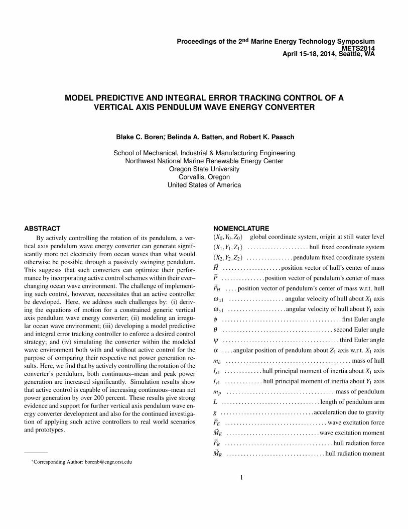
Given an appropriate mooring scheme, the genericVAPWEC can be constrained to move in large part in only heave,roll, and pitch. Thus, with the inclusion of pendulum motion, thegeneric VAPWEC modeled has four dominant degrees of free-dom. Figure 2 shows a free body diagram illustrating the dynam-ics of the constrained VAPWEC. The equations of motion for theVAPWEC are derived using Newtonian mechanics with the aidof three coordinate systems: global fixed, hull fixed, and pendu-lum fixed coordinate systems. Using the z-x′-z′′ sequence, Eulerangles φ , θ , and ψ are employed to relate the angular orientationof the VAPWEC’s hull and, indirectly, the VAPWEC pendulum’sposition to the global coordinate system, see [10, 11]. Here weconsider six main forces or moments affecting the VAPWEC:(i) wave excitation force ~FE and moment ~ME ; (ii) wave radiationforce ~FR and moment ~MR; (iii) weight of the hull mh~g; (iv) weightof the pendulum mp~g; (v) pendulum viscous damping moment~Md ; and (vi) pendulum generator moment ~Mgen.

The equation of motion for the hull moving along the Z0 axis

3

X0

Z0

ME + MR

mp g

FE + FR

X1

Z1 & Z2

Hcom Pcom

X1

Y1

Y2 X2

Md + Mgen

mh g

Side View

Top View

IrregularWave Profile

PH

α

Wave Progression

Hull

Pendulum

PH

H

Pcom

Hcom

FIGURE 2. VAPWEC FREE BODY DIAGRAM

is given by

Hz0 =−mh g−mp g+FEz0 +FRz0

mh. (1)

The equation of motion for the hull rotating about the X1 axis andthe Y1 axis, respectively, are given by

ω x1 =MEx1 +MRx1 +Rpy0 mp g

Ix1(2)

and

ω y1 =MEy1 +MRy1 −Rpx0 mp g

Iy1. (3)

The equations of motion defining the hull’s orientation withrespect to the global coordinate system (the hull’s Euler angles)

are given by

φ =ω y1 cos(ψ)+ω x1 sin(ψ)

sin(θ), (4)

θ = ω x1 cos(ψ)−ω y1 sin(ψ) , (5)

and

ψ =–cos(θ)

(ω y1 cos(ψ)+ω x1 sin(ψ)

)sin(θ)

. (6)

The equation of motion defining the pendulum’s rotationabout the Z1 axis is given by

α =sin(2 α)

(ω2

x1−ω2

y1

)2

− cos(2 α)ω x1 ω y1

+

(Md +Mgen−L mp cos(α +ψ) sin(θ)

(g+ Hz0

))L2 mp

(7)

where

Md =−Cp α , (8)

and

Mgen = u(t) . (9)

Note, control is to be implemented through generator feedback,see Eqn. (9). When Mgen opposes pendulum motion, electricityis being generated and energy is removed from the pendulum(generator mode). When Mgen aids the motion of the pendulum,energy is being transferred to the pendulum (motor mode).

Simulated Hydrodynamic EnvironmentThe Pacific Northwest is a site of interest for WEC develop-

ment, and as such the simulated irregular hydrodynamic wave en-vironment is based on characteristics suitable for WEC develop-ment for Oregon State oceans. The irregular wave’s spectrum isderived using the Modified Bretschneider-Mitsuyasu wave spec-trum given by [12, 13]

S( f j) = 0.205 H2s T−4

s f−5j exp

(−0.75 (Ts f j)

−4) . (10)

4

The spectrum is generated using a significant wave height,Hs, of three meters and a significant wave period, Ts, of ten sec-onds. Such wave parameters can be considered the most appro-priate and representative for WEC development off the coast ofOregon [9]. The resulting irregular wave form developed fromthe spectrum is due to the superposition of individual, monochro-matic water surface elevations, η j, and is given by

~ηirr =N

∑j=1

~η j =N

∑j=1

cos(k j x0 − 2π f j t−δ j) . (11)

For the generic VAPWEC simulations, a simple method isused for determining both the excitation force, ~FE , and the ex-citation moment, ~ME . The method leverages Froude–Krylovforcing and, is thus directly related to Eqn. 11. This methodassumes a floating body to have negligible diffraction effects.Such an assumption is valid if the floating body is relativelysmall when compared to the wave’s dominant wavelength andalso valid when only a first order approximation of the excitationforce is needed—as is the case for this work [14–17]. To facil-itate the Froude–Krylov criterion, the modeled VAPWEC hullhas a height of 2.5 meters and a diameter of 10 meters. Theestablished hull size is much smaller than the irregular wave’s150 meter approximate significant wavelength, and is also largeenough that viscous effects (due to flow separation) can be ne-glected [16, 17]. Ultimately, the needed excitation force, ~FE , andmoment, ~ME , can be obtained through use of the aforementionedFroude–Krylov method by integrating the irregular wave’s pres-sure field over the wetted surface area of the VAPWEC,

pirr =N

∑j=1−ρ gz0 +ρ gη j Kp j (12)

where

Kp j =cosh

(k j(h+ z0)

)cosh(k jh)

. (13)

To simplify the integration of the pressure field over the con-tinually changing wetted surface area of the modeled VAPWEC,the process is approximated by dividing the hull into four (A, B,C, and D) symmetric wedges, with each wedge having its ownexcitation force, see Figure 3. The respective excitation force ofeach wedge is a product of two components: (i) one fourth theweight of the hull and (ii) a scaled sigmoid function. The combi-nation of these two components result in the following equation:

~FN =

(mh g

4

) ( 2

1+ exp(−A f ~dN)

)

=mh g

2(

1+ exp(−~dN)) (14)

where

N = A, B, C, D ,

~dN =~ηN−~RNz0 , (15)

and

~ηN =~ηirr

(x0 = RNx0

). (16)

FC

FB

FD

FA

X1

Z1

Y1

FIGURE 3. VAPWEC HULL WEDGES AND CORRESPONDINGWAVE EXCITATION FORCES

The value of the sigmoid scaling function is what ultimatelyapproximates the pressure field integration process and whosevalue is determined by how much a respective wedge is sub-merged below the irregular wave profile, ~ηirr, see Figure 4. Thesigmoid scaling function acts such that when the hull is halfway submerged in still water, the sum of each wedge’s excita-tion force is equal to the total weight of the VAPWEC’s hull.Thus, the hull’s nominal hydrostatic condition, without the pen-dulum, is half submergence. As each wedge’s submergence in-evitably increases or decreases, due to the hull being subjected tothe irregular wave, ~ηirr, and the pendulum dynamics, ~α , the con-tribution of each respective wedge excitation force is adjustedaccordingly. In other words, as a wedge becomes increasinglymore submerged, its corresponding excitation force is increased,but only until the wedge is completely submerged. After com-plete submergence, the wedge’s corresponding excitation forceno longer increases. Likewise, when a wedge becomes decreas-ingly less submerged, its corresponding excitation force is de-creased, and can be decreased until zero which represents the

5

point where the majority of the wedge is unsubmerged. See Fig-ures 3 and 4. Based on comparable ANSYS AQWA R© analyses,this sigmoid function approximation technique gives the approx-imate excitation force, ~FE , and moment, ~ME sufficient for thiswork:

~FE = ~FA +~FB +~FC +~FD , (17)

and

~ME =D

∑N=A

(~RN×~FN

). (18)

Irregular W

ave Profile

X1

FA

Z1

RA

dA

ηA

X0

Z0

Wedge “A” of Hull

H

FIGURE 4. WEDGE “A” OF VAPWEC HULL

The radiation force, ~FR, and moment, ~MR, were found us-ing a method from [18] and further supplemented by ANSYSAQWA R©. ANSYS AQWA R© was not solely used for the analy-sis in this work due to its several inabilities to handle advancedcontrol algorithms such as what will be describe in a subsequentsection. Note, the radiation force and moment can be expandedand related to the constrained motion of the modeled VAPWECby the following:

~FRz0=−Cz0

~Hz0−Az0~Hz0 , (19)

~MRx1 =−Cx1 ωx1−Ax1 ωx1 , (20)

~MRy1 =−Cy1 ωy1 −Ay1 ωy1 . (21)

A summary of the hydrodynamic and VAPWEC parametersused in this work are given in Table 1.

Active Controller DesignUsing both model predictive and integral error control, a

controller is developed to enforce a strategy that optimizes waveenergy to electricity conversion. Such a controller is ideally

TABLE 1. SUMMARY OF HYDRODYNAMIC AND VAPWEC PA-RAMETERS

Parameter Value

Significant Wave Height 3 [m]

Significant Wave Period 10 [s]

Hull Mass 10000 [kg]

Hull Principal moment of inertia about X1 129709 [kg m2]

Hull Principal moment of inertia about Y1 129709 [kg m2]

Hull Diameter 10 [m]

Hull Height 2.5 [m]

Sigmoid Approximation Factor 1

Pendulum Arm Length 3 [m]

Pendulum Mass 250 [kg]

Pendulum Damping Coefficient 0.1[kg m2 s−1]

Hull Added Mass in Heave 109346 [kg]

Hull Added Inertia in Roll 385027[kg m2]

Hull Added Inertia in Pitch 385027[kg m2]

Radiation Damping in Heave 51252[kg s−1]

Radiation Damping in Roll 2578[kg m2 s−1]

Radiation Damping in Pitch 2578[kg m2 s−1]

suited for this problem due to its ability to cope with approxi-mated nonlinear dynamics, its capacity to track desired pendu-lum state trajectories, and its allowance for wave profile predic-tion [5, 6, 19].

The model predictive control aspect grants the controller ameans to continually update the approximation of the nonlinearpendulum dynamics in a manner that allows for the applicationof linear optimal control theories for discrete moments in time.Such approximation enables the direct use of common linearcontrol methods which are easily computed and implemented.Moreover, model predictive control provides a means for futureresearch in which temporal and spacial wave profile predictioncan occur [7]. With integral error control, the controller has theability to track a desired ideal pendulum state trajectory. Thecontroller combines the model predictive and integral error con-trol aspects via an augmented state-space equation and a corre-sponding cost function that is analogous to linear quadratic reg-ulator (LQR) problems.

A linear approximation to the pendulum dynamics in (7) canbe written in a time-varying form that uses the current time win-dow’s (ti) state values:

ϒϒϒ(t) = AAAmpc(t)ϒϒϒ(t)+BBB u(t) (22)

6

where

AAAmpc(t) =

−Cx1Ix1

0 0 0

0−Cy1

Iy10 0

0 0 0 1

A41(ti) A42(ti) A43(ti)−Cp

L2 mp

, (23)

A41 =sin(2α(ti)

)ωx1(ti)

2, (24)

A42 =cos(2α(ti)

)ωx1(ti)− sin

(2α(ti)

)ωy1(ti)

2, (25)

A43 =

sin(α(ti)+ψ(ti)) sin(θ(ti)

) (g+ FHz0(ti)

mh

)L

, (26)

ϒϒϒ(t) =[

ωx1(t) ωy1(t) α(t) α(t)]T , (27)

BBB =

[0 0 0 1

L2 mp

]T

, (28)

and recalling u(t) = Mgen(t) .

The pendulum state matrix, AAAmpc, could include any infor-mation for the intention of prediction and approximation. In-formation such as: historic, current, predicted state informa-tion; historic, current, predicted control information; or predictedwave environment and hull forcing information. The inclusionand investigation of using of such information for AAAmpc, is a nat-ural path for future research. As it stands, the linear approxima-tion of AAAmpc used in this work, only includes hull and pendulumstate information from the current time window, ti.

As noted earlier, pendulum control is effectuated throughgenerator torque feedback. When the moment due to the genera-tor, Mgen, opposes the pendulum’s angular velocity, α , electricityis being generated. When the moment due to the generator, Mgen,aids the pendulum’s angular velocity, α , the generator is actingas a motor and electricity is being consumed.

The control strategy enforced by the active controller isbased on tracking a desired pendulum state trajectory, r(t). The

reference function r(t) is found through an iterative process suchthat a favorable trajectory is found for the aforementioned sim-ulated irregular ocean wave environment. A specific method forascertaining r(t) is described by Boren and its purpose is to in-form the controller of proper pendulum orientation throughouttime such that pendulum motion optimizes wave energy to elec-tricity generation [5].

Tracking the ideal pendulum state trajectory, r(t), is the pri-mary role of the integral error component of the controller [5,20].Such tracking involves the minimization of the pendulum’s errordynamics given by

e(t) = r(t)−α(t). (29)

When written in state–space form the error dynamics in Eqn.(29) becomes

e(t) =−CCC ϒϒϒ(t)+ r(t), (30)

CCC =[0 0 1 0

]. (31)

Thus, the augmented state–space form for the controller isthe combination of the approximated pendulum state-space dy-namics and the integral error dynamics. The resulting augmentedstate-space form is given by

[ϒϒϒ(t)e(t)

]=

[AAAmpc(t) 000−CCC 0

][ϒϒϒ(t)

e(t)

]

+

[BBB

0

]u(t)+

[0001

]r(t) (32)

or

ϒϒϒaug(t) = AAAaug(t)ϒϒϒaug(t) (33)

+BBBaugu(t)+[

0001

]r(t)

as in [20]. Note that the zero entries in the matrices above aresized appropriately; that is, they may represent vectors or sub–matrices with zero entries.

The controller is derived using a linear quadratic cost func-tion given as

Ji =

∫∞

ti

ϒϒϒTaug(t)QQQϒϒϒaug(t)+uT (t)Ru(t)dt (34)

7

with

QQQ =

[000 000000 q

]. (35)

The terms R and q represent control weighting and errorweighting respectively. Small R values allow for greater pen-dulum control to be implemented, and correspondingly, larger qvalues enforce closer tracking of the function r(t). These weight-ings are typically “tuned” to achieve desired performance.

To ensure suitable control of the pendulum and sufficienttracking of r(t), Eqn. (34) is minimized by solving its corre-sponding steady state algebraic Riccati equation

000 =−PPPAAAaug−AAATaugPPP−QQQ+PPPBBBaugR−1BBBaug

T PPP (36)

at sequential time moments in time, t. Thus, PPP in fact dependson t. At each time t, its associated gain matrix, KKK(t), is derivedby

−KKK(t) =−R−1 BBBaugT PPP(t) , (37)

and thus over the entire operating time,

u(t) = Mgen(t) = −KKK(t)ϒϒϒaug(t) . (38)

SIMULATION RESULTSUtilizing the same simulated irregular ocean wave, hydro-

dynamic environment, and VAPWEC parameters(see Table 1,

Eqns. (1)–(9) and Eqns. (11)–(21)), the results of two simu-

lations are now given. The first simulation places the modeledVAPWEC in the simulated ocean environment without activecontrol enabled. The second simulation places the same modeledVAPWEC in the same simulated ocean environment, but with theactive controller developed by Eqns. (22)–(38), enabled. The re-sulting net power produced from each simulation is comparedand, in this fashion, the benefits of using active control are as-sessed. The governing evaluation of the active controller is basedupon its ability to increase net power output as compared to itsuncontrolled counterpart.

The duration of each simulation is 1200 seconds with onlythe last 100 seconds of power generation being considered forevaluation. In this way, the evaluation is based upon the fullydeveloped interactions between the irregular wave environmentand the VAPWEC’s dynamics—disregarding the transient effectsthat occur during the sudden placement of a VAPWEC into an al-ready existing dynamic ocean wave environment. Note, positivepower represents electricity generation by the VAPWEC (genera-tor mode), while negative power represents electricity consump-tion by the VAPWEC (motor mode).

Generic VAPWEC without Active ControlWithout active control, a VAPWEC generates electricity at

a linear rate. This rate is a product of a predetermined extractioncoefficient, Cgen, and the VAPWEC pendulum’s angular velocity,α . This relationship is given by

~Mgen(t) =Cgenα(t) . (39)

Thus, for electricity generation to occur, Cgen, must be a nega-tive value and also a quantity that facilitates the largest amountof electricity generation. The determination of Cgen is ordinarilybased on the converter’s physical parameters in addition to thedominant characteristics of the converter’s ocean wave energyenvironment. In the case of this simulation, Cgen was found byiteratively subjecting the modeled VAPWEC to the same irreg-ular ocean wave while searching through a range of Cgen valuesbetween -80000 and 0

[kg m 2 s−1

]. From this process a value

of -29091[kg m 2 s−1

]was found to generate the largest amount

of electricity for the uncontrolled VAPWEC during the last 100seconds of simulation time.

The simulation results for the uncontrolled VAPWEC, forthe last 100 seconds are summarized in Figure 5 and its cor-responding power generation results are given in Table 2. Asshown in the power plot of Figure 5, by having a negative extrac-tion coefficient, Cgen, the VAPWEC without active control willalways generate electricity during any pendulum motion. More-over, greater electric power generation is associated with fasterpendulum rotation, which is indicated by steeper slopes in thependulum position plot of Figure 5 and implied by Eqn. (39).Mean net continuous power output for the last 100 seconds ofsimulation time was only 382 watts—small considering the large10 meter diameter of the VAPWEC’s hull. This small result,however, is due to the generic form of the modeled VAPWEC. Ifone were to optimize the VAPWEC hull’s geometry and pendu-lum parameters, than greater power output, even for an uncon-trolled VAPWEC, could be had. In any case, it is the purpose ofthis work to focus on the comparison between an uncontrolledand active controlled VAPWEC without favor towards a particu-lar VAPWEC design or configuration.

TABLE 2. RESULTS: WITHOUT ACTIVE CONTROL

Parameter Value

Generator Extraction Coefficient -29091[kg m 2 s−1]

Mean Net, Continuous Power (during last 100seconds)

382 [W]

Max Net, Peak Power (during last 100 seconds) 1,757 [W]

8

1100 1110 1120 1130 1140 1150 1160 1170 1180 1190 12000

1000

2000

[w]

1100 1110 1120 1130 1140 1150 1160 1170 1180 1190 1200−4

−2

0

1100 1110 1120 1130 1140 1150 1160 1170 1180 1190 1200−5

0

5

Time [s]

[m]

Water Surface Elevation (η )Vertical Position of Hull in Heave

[rad

s]

Pendulum Position

Power

FIGURE 5. VAPWEC WITHOUT ACTIVE CONTROL

Generic VAPWEC With Active ControlTo simulate an actively controlled VAPWEC, an optimal

pendulum state trajectory, r(t), must be identified. While therecould be several possibilities for r(t), for this simulation, a sim-ple sinusoid was found to be an effective optimal pendulum statetrajectory. The sinusoid is given by

r(t) = 3sin(t) . (40)

In addition to the optimal pendulum state trajectory, the ac-tive controller was forced to favor electricity generation overelectricity consumption. Thus, whenever the controller soughtto add energy to the system, it was only allowed to do so at 80percent of its desired amount. The active control moment, u(t),therefore, is given by

u(t) = Mgen(t)

= −KKK(t)ϒϒϒaug(t) when ±Mgen & ∓ α (41)

and

u(t) = 0.8 Mgen(t)

= −0.8 KKK(t)ϒϒϒaug(t) when ±Mgen & ± α (42)

When compared to the power results of the uncontrolledVAPWEC simulation (Figure 5 and Table 2), the results from theactively controlled VAPWEC simulation (see Figure 6 and Ta-ble 3) indicate both greater peak power outputs and continuous–mean power output. Due to the nature of active control however,electric power generation does not always occur. Thus, while ac-tive control produced large spikes—nearly 0.5 [MW]—of power

at certain times, its continuous–mean power output was approx-imately 1.5 [kW]. Nonetheless, in terms of continuous–meanpower output, the actively controlled VAPWEC outperforms itsuncontrolled counterpart by nearly 1 [kW] of continuous–meanpower output.

1100 1110 1120 1130 1140 1150 1160 1170 1180 1190 1200−5

0

5 x 105

[w]

1100 1110 1120 1130 1140 1150 1160 1170 1180 1190 1200−5

0

5

1100 1110 1120 1130 1140 1150 1160 1170 1180 1190 1200−5

0

5

Time [s]

Water Surface Elevation (η )Vertical Position of Hull in Heave

[rad

s][m

]

Pendulum Position

Power

FIGURE 6. VAPWEC WITH ACTIVE CONTROL

TABLE 3. RESULTS: WITH ACTIVE CONTROL

Parameter Value

Selected Optimal Pendulum State Trajectory r(t) = 3sin(t) [m]

Error weighting q 1e13

Control weighting R 1e-11

Mean Net, Continuous Power (during last 100seconds)

1,473 [W]

Max Net, Peak Power (during last 100 seconds) 493,080 [W]

CONCLUSIONSIn this paper, we have shown that net mean power generation

for a VAPWEC could be increased by over 200% by utilizingan active controller based on model predictive and integral errortracking control theories. Such an approach to control design hasbeen used by others for other technologies, and is a realistic firsttake for controlling both VAPWECs and wave energy convertersin general [1, 5, 6].

Another contribution in this paper, is the simplified approachto modeling the hydrodynamic forcing on the device. Initially,panel methods and ANSYS AQWA R© were used to both com-pute the hydrodynamic forces and apply active control to theVAPWEC [5, 21], but that approach proved to be entirely un-wieldy due to AQWA’s inadequate interface for active controltechniques. The approach used in this paper is essentially away to average the hydrodynamic forces over quadrants of the

9

VAPWEC, and could be refined by partitioning the device intomore wedges.

A possible limitation regarding the use of such active con-trol, are the resulting large power spikes. Here we assume anideal power take–off system, a system capable of handling thetransmission of power of up to nearly 500 kilowatts. However,these large power spikes need not be prohibitive, especially ifsuch spikes are only allowed in generator mode (no need tosource large amounts of power) and if they last for very brieftime periods.

Another possible limitation regarding the use of active con-trol, is the assumed forward knowledge of the incident, incomingirregular wave form. Such a limitation, however, could be sur-mounted through the use of state estimators that transmit wavetelemetry to the controller such that the controller can make rea-sonable predictions about the future incident wave. Such estima-tors are currently being investigated by the authors of this work.

An additional area for future work in VAPWEC control de-sign, involves utilizing cost functions that do not require trackingof an desired pendulum position, r(t), but instead the controllerwould continually develop, in essence, r(t), on–the–fly. Suchreal–time tracking function development is being investigated bythe authors of this work.

ACKNOWLEDGMENTThe material in this paper is based upon work supported by

the US Department of Energy under Award Number DEFG36-08GO18179.

REFERENCES[1] Previsic, M., 2013. “The potential of wave power in

the United States in an economic context”. In Track 10:EWTEC 2014, The European Wave and Tidal Energy Con-ference.

[2] Bull, D., Ochs, M., Laird, D., Boren, B., and Jepsen, R.,2013. Technological cost-reduction pathways for point ab-sorber wave energy converters in the marine hydrokineticenvironment. Tech. rep., Sandia National Laboratories.

[3] Hinck III, E. C., 1966. Wave power generator, January.United States Patent: 3231749.

[4] Bretl, J. G., 2009. “A time domain model for wave inducedmotions coupled to energy extraction”. PhD thesis, TheUniversity of Michigan.

[5] Boren, B. C., 2013. “On the modeling and control of hori-zontal pendulum wave energy converters”. Master’s thesis,Oregon State University, June.

[6] Brekken, T. K. A., 2011. “On model predictive control fora point absorber wave energy converter”. In PowerTech, 1,pp. 1–8.

[7] Wang, L., 2009. Model Predictive Control System Designand Implementation Using MATLAB R©. Advances in In-dustrial Control. Springer.

[8] Findeisen, R., Allgower, F., and Biegler, L., 2007. Assess-ment and Future Directions of Nonlinear Model PredictiveControl. Lecture notes in control and information sciences.Springer.

[9] Lenee-Bluhm, P., 2010. “The wave energy resource of theU.S. pacific northwest”. Master’s thesis, Oregon State Uni-versity.

[10] Altmann, S., 2005. Rotations, Quaternions, and DoubleGroups. Dover books on mathematics. Dover Publications.

[11] Kuipers, J., 1999. Quaternions and Rotation Sequences: APrimer With Applications to Orbits, Aerospace and VirtualReality. Mathematical Sciences Series. Princeton Univer-sity Press.

[12] Goda, Y., 2010. Random Seas and Design of MaritimeStructures (3rd Edition). Advanced series on ocean en-gineering. World Scientific Publishing Company, Incorpo-rated.

[13] Goda, Y., 1988. “Statistical variability of sea state parame-ters as a function of a wave spectrum”. Coastal Engineeringin Japan, 31, pp. 39–52.

[14] Dean, R., and Dalrymple, R., 1991. Water Wave Mechanicsfor Engineers and Scientists. Advanced series on oceanengineering. World Scientific.

[15] Newman, J., 1977. Marine Hydrodynamics. Wei ChengCultural Enterprise Company.

[16] Sarpkaya, T., 2010. Wave Forces on Offshore Structures.Wave Forces on Offshore Structures. Cambridge UniversityPress.

[17] Wilson, J., 2003. Dynamics of Offshore Structures. Wiley.[18] Ghadimi, P., Bandari, H., and Rostami, A., 2012. “Deter-

mination of the heave and pitch motions of a floating cylin-der by analytical solution of its diffraction problem and ex-amination of the effects of geometric parameters on its dy-namics in regular waves”. International Journal of AppliedMathematical Research, 4, pp. 611–633.

[19] Rawlings, J., and Mayne, D., 2009. Model Predictive Con-trol: Theory and Design. Nob Hill Publishing.

[20] Burl, J., 1999. Linear optimal control: H2 and H∞ methods.Addison Wesley Publishing Company Incorporated.

[21] Chakrabarti, S., 2005. Numerical Models in Fluid-Structure Interaction. Advances in Fluid Mechanics. WITPress.

10