MODEL ORGANIC RANKINE CYCLE FOR BRINE AT … ORGANIC RANKINE CYCLE FOR BRINE AT OLKARIA GEOTHERMAL FIELD, KENYA ... An internal report from KenGen’s ... the pump outlet assuming

Orkustofnun, Grensasvegur 9, Reports 2016 IS-108 Reykjavik, Iceland Number 15

227

MODEL ORGANIC RANKINE CYCLE FOR BRINE AT OLKARIA GEOTHERMAL FIELD, KENYA

Gideon Gitonga Gitobu Kenya Electricity Generating Company Ltd. - KenGen

P.O. BOX 785 – 20117, Naivasha KENYA

[email protected], [email protected]

ABSTRACT A mix of conventional and wellhead power plants is used to generate geothermal power at Olkaria. All these plants utilize only the steam phase of the geothermal fluid flashing process. As a result, huge volumes of brine are left behind which if utilized can extend the exploitable potential of the field. This is possible using organic Rankine cycle (ORC) power plants that have been used successfully all over the world as bottoming units for conventional geothermal power plants. Every installation of organic Rankine cycle power plant requires a custom design tailored to suit the particular conditions of the source fluid and ambient climatic conditions. This paper models a suitable power plant for installation at the combined brine stream from separator stations SD2 and SD3 in Olkaria IV field bound for reinjection to well OW-911. The scope covered here is the design and sizing of major plant components from which it has been estimated that an ORC plant running on n-pentane as the working fluid installed on this brine stream will have a gross capacity of 4.6 MW and cost about 2,202 USD/kW. The cost is low because the installation of a bottoming ORC plant usually comes at such a time when the major geothermal development cost has been assigned to the conventional power plants. Therefore, it is the key finding of this paper that in a well-developed geothermal field like Olkaria, bottoming ORC plants can generate extra power at an economically competitive cost.

1. INTRODUCTION 1.1 Current geothermal development status Commercial geothermal operation started in Olkaria in 1981. Since then the installed capacity has increased and currently KenGen owns and operates 4 conventional power plants and 15 wellhead units in Olkaria with a total installed capacity of 505 MW. All of these power plants utilize the single flash steam cycle technology. The principle here is to flash the geothermal fluid in a separator to harness steam that goes to the power plant for power production while brine is re-injected into the reservoir. The total separated brine is 2729 t/hr (Table 1) and could be used to produce power using organic Rankine cycle (ORC) plants. The steam field systems serving different power plants are not exactly similar and due to this the separated brine has different properties. These properties affect the relative feasibilities of utilization of the separated brine. An internal report from KenGen’s Board of Consultants

Gitobu 228 Report 15

in April, 2016 recommended that consideration should be given to the installation of bottoming cycle generation at those power plants where brine temperature remains high after separation (KenGen, 2016). This forms the basis of this project which is to explore how to optimally utilize brine for power generation in Olkaria. Preliminarily, an overall status of all separated brine in Olkaria field will be reviewed. Then the centre piece of this paper will be to model an ORC plant on the location with the best combination of factors such as availability of sufficient brine, ease of power evacuation, minimal environmental impact and existing road network. 1.2 Project justification As explained above, KenGen currently uses a mix of conventional power plants and wellhead power plants for power production. The designed operating conditions for these plants are different for each one because it is important to match the plant design to the reservoir properties from which the geothermal fluids are tapped. Secondary design optimizations have continuously been pursued and adopted in a bid to bring down overall project costs and keep environmental effects to a minimum. Owing to this, plants are designed differently and besides that the design of pioneer geothermal plants is quite different from the modern ones due to technological advancements. As a result, for instance each plant in Olkaria has a distinct steam gathering system with different layouts and different operating conditions. The main features for Olkaria I and II power plants are that they have one main separator for each well and the separation pressure is about 6.0 bar-a. The new power plants Olkaria IV and Olkaria I additional units 4 and 5 have central separator stations and the separation pressure is about 12 bar-a. The wellhead plants are modular installations mostly fed by one well although in some cases one powerful well can serve two units. The separation pressure for the wellheads is about 15 bar-a. The separated brine is summarized in Table 1 below according to plants.

TABLE 1: Brine mass flows and properties

Plant Brine (t/hr) Separation pressure (bar-a) Brine temperature (°C) Olkaria I 235 6 158.9 Olkaria II 566 6 158.9 Olkaria IAU 524 12 188 Olkaria IV 815 12 188 Wellheads 589 15 198.3

In principle, it is possible to use all the separated brine for power generation. However, distinct conditions for each field cause the brine which is available to have different utilization potentials. Olkaria I has a partial reinjection scheme that encompasses a hot reinjection system and an open disposal to a lagoon from where it is pumped and used for drilling. Since the brine reinjection system for Olkaria I field is not much integrated, the cost of consolidating the brine together for power generation hugely undermines the economic feasibility of such an undertaking. The scattered nature of the wellheads and the possibility that they can be moved to a new location on a need basis discounts the prospect of having a bottoming cycle on them. Another factor that has to be taken into consideration is that KenGen is licensed to carry out exploitation and development in Olkaria geothermal field that cover about 204 km2 and a part of this area lies within the Hells Gate National park. The National park plays a major role in the tourism industry which is a key economic booster in the area. Geothermal development activities and wildlife conflicts have always been kept to a minimum. Olkaria II and Olkaria IAU have well integrated steamfield systems with large brine flows at particular locations but lie within the game park. This paper does not conclude that it is difficult to install an ORC plant anywhere within Olkaria geothermal field. But it recognizes that one of the most ideal places for installation of an ORC plant is Olkaria IV field, the brine stream to reinjection well OW-911. This is the brine stream with the largest mass flow (499.5 t/hr) at a temperature of 188°C and it receives brine from separators stations SD2 and SD3 in Olkaria IV field (Figure 1). An ORC power plant for installation on this brine stream will be modelled here.

Report 15 229 Gitobu

FIGURE 1: Location of separator stations SD2 and SD3 and hot reinjection well OW-911

1.3 Project scope The scope of the project involves process design and sizing of major system components which then will give a reasonable clue to the expected project cost. In its basic form, a binary power plant under consideration here follows the schematic shown in Figure 2 below. 2. REVIEW OF RELATED LITERATURE 2.1 Thermodynamic cycle analysis Process description in this section will refer to Figure 2. An organic Rankine cycle plant can basically be divided into three technical subsystems: the geothermal fluid or brine in this case, the power conversion cycle and the cooling system for the removal of heat (Frick et al., 2015). In a good design the three subsystems should interact reliably, efficiently and economically. In regard to the three subsystems, the basic theory of an ORC plant is that a working fluid chosen for its appropriate thermodynamic properties is fed to the heat exchanger where it receives heat from the geothermal fluid, expands through the turbine, condenses and then is fed back to the heat exchangers by a feed pump. ORC is a closed loop system and to have sequential description of the system this paper will describe the cycle the working fluid undergoes from the feed pump until it comes back to the same point again. DiPippo (2007) provided the basis of this description of the ORC system alongside the equations to be used in the analysis. It is assumed that the cycle runs in a steady state condition with no system pressure drop except across the turbine inlet valve and negligible kinetic and potential energies. 2.1.1 Feed pump The enthalpy increase due to pressure differences across the pump and the pumping power can be obtained by Equations 1 and 2, respectively.


( – ) = ( – ) (1) = wf( – ) = wf ( – )/ η (2) where and are the working fluid enthalpy at the feed pump outlet and at the inlet respectively, is the specific volume, and refers to the pressure at the pump outlet and inlet respectively, is the working fluid enthalpy at the pump outlet assuming an isentropic process and η is the isentropic pump efficiency. Eastop and MacConkey (1993) showed that for a liquid that is assumed to be incompressible (i.e. = constant), the enthalpy change due to isentropic compression is given by: (3) 2.1.2 Heat exchanger The heat exchanger is composed of the preheater and the evaporator. The design of heat exchangers requires examination of the temperature - heat transfer (T-q) diagram shown in Figure 3. FIGURE 3: Preheater and evaporator T-q diagram

FIGURE 2: Schematic diagram showing brine source and ORC plant


The brine transfers heat to the working fluid in a process that can be described as follows. Preheater In the preheater, the working fluid flows in the shell while the brine flows in the tubes. The movement of the working fluid in the shell is guided by baffles. The preheater heats up the working fluid to almost boiling point. That small margin to the boiling temperature in the preheater ensures that vapour doesn’t form and gets locked in the baffles. Heat transfer process in the preheater is governed by this heat mass balance equation: b( – ) = wf ( – ) (4) where and refers to the brine enthalpy as it enters and leaves the preheater respectively while

and refers to the working fluid enthalpy as it enters and leaves the preheater respectively. Evaporator In the evaporator, the working fluid receives sensible heat up to the boiling point (bubble point), then latent heat up to vapour saturation (dew point) and additional heat up to 2°C superheat. Therefore, the heat duty of the evaporator is the sum of those three heat components whose mass balance equations are explained below:

Sensible heat required to raise fluid temperature from the preheater outlet temperature up to its boiling point:

b( – ) = wf ( – ) (5) where and refer to the brine enthalpy at the evaporator bubble point and exit point respectively while and refer to the working fluid enthalpy at the evaporator entry and bubble point respectively.

Latent heat required to vaporize the working fluid from the boiling point to vapour saturation point:

b( – ) = wf ( – ) (6) where and refer to the brine enthalpy at the evaporator dew point and bubble point respectively while and refer to the working fluid enthalpy at the evaporator bubble point and evaporator dew point respectively.

Heat required to superheat the working fluid to 2°C: b( – ) = wf ( – ) (7) where and refer to the brine enthalpy at the evaporator entry and dew point while and refer to the working fluid enthalpy at the evaporator dew point and evaporator exit point respectively. 2.1.3 Turbine The turbine extracts energy from the working fluid. One thing to note here is that there is a pressure drop across the turbine inlet valve estimated at 0.3 bar. This throttling process is isenthalpic and so the turbine inlet enthalpy is the same as the enthalpy at the evaporator outlet. There will however be a slight drop in working fluid temperature between state point 5 and 6 as will be shown in Figures 8 and 9 due to this reduction in pressure. The turbine power is given by:


t = wf( – ) = wf η ( – ) (8) where is the vapour enthalpy at turbine inlet, is the actual vapor enthalpy at the turbine outlet, η is the turbine efficiency and is the vapor enthalpy at the turbine outlet assuming isentropic process. The turbine efficiency is given by the manufacturer and it is the ratio between the real enthalpy change through the turbine to the largest possible (isentropic) enthalpy change (Valdimarsson, 2011). 2.1.4 Condenser This is where the heat is rejected from the working fluid to the cooling medium which is air in this case. If a dry working fluid is used it exits the turbine in a superheated state. Condensation then is in two stages according to the T-q diagram (Figure 4). The first stage is to de-superheat the fluid to its dew point and the second stage is to remove the latent heat up to liquid saturation. The heat which is rejected in the condenser to de-superheat the working fluid to its dew point is given by: wf( – ) = cond_air ( – ) (9) Where is the working fluid enthalpy at the turbine outlet, is the working fluid enthalpy at condenser dew point, cond_air is the cooling air mass flow rate, is the constant specific heat of air while and refer to the cooling air temperature at the condenser dew-point and exit point respectively. The latent heat which is rejected by the working fluid to condense it from dew point to liquid saturation is given by: wf( – ) = cond_air ( – ) (10) Where is the working fluid enthalpy at condenser outlet and refers to the cooling air temperature as it enters the condenser, which is the same as ambient air temperature. The other parameters are as described in Equation 9 above. 2.2 Heat transfer area calculation In the preheater and evaporator heat is transferred to the working fluid over a surface area. The same principle applies in the condenser where cooling air draws heat from the working fluid over a surface and cools it as a result. The heat transfer area between two fluids is determined by the following heat transfer equation:

FIGURE 4: Condenser T-q diagram


∙ ∙ (11)

where is the overall heat transfer coefficient (Table 2 below shows assumed values for this model), is the heat transfer area and is the log mean temperature difference which is obtained from the formula below:

(12)

where is the temperature difference between the two streams at end A and is the temperature difference between the two streams at end B (Wikipedia, 2016a). In the preheater, the working fluid temperature is raised linearly so the heat transfer area calculation is a straightforward application of equations 11 and 12. However in the evaporator, the working fluid temperature increase is non-linear since there is a heat component that heats the fluid to boiling point, another heat component heats the fluid up to the dew point and finally some heat is required to superheat the fluid (Figure 3). This means the LMTD and therefore heat transfer area is calculated separately for these three parts and summed up to get the total evaporator heat transfer area. In the condenser, the working fluid temperature decreases in a non-linear manner as shown in the T-q diagram (Figure 4). This is because there is a component of heat that is removed from the fluid to de-superheat it to condenser dew point and then latent heat must be extracted to cool it to liquid saturation point. Therefore, the LMTD and heat transfer area is calculated separately for these two parts and summed up to get the total condenser heat transfer area. The evaporator and the condenser have pinch points where the temperature difference between the two fluids’ exchanging heats is minimum. The choice of the pinch affects the overall performance and cost of the plant and therefore its choice is the result of economic optimization. A small pinch increases the performance of the heat exchanger and the condenser but it is costlier. A large pinch corresponds to the smaller and less costly heat exchanger and condenser but with reduced thermal performance. 2.3 Calculation of the parasitic load The two components that consume the bulk of the auxiliary power are the feed pump and the condenser cooling fans. Feed pump power consumption has been explained in Equation 2. Due to the scarcity of water around the project area an air-cooled condenser is considered here. According to Wolverine (2016) the fan power required to move air through the heat exchanger is:

(13)

where is the mass flux at minimum flow cross section area, which is given by G = ,

being mass flowrate of air and is the cooling air pressure drop across the heat exchanger while is the density of air. The ratio of mass to density is the same as volume. With that, Equation 13 can be rewritten as follows:

TABLE 2: Heat transfer coefficients (Fernando, 2013)

Component (KW/m2°C)

Preheater 1 Evaporator 1.6 Air condenser 0.8


(14)

where is the efficiency of the cooling tower fan. 3. SELECTION OF THE WORKING FLUID Appropriate selection of a working fluid is an important matter because it has great implications on the performance of a binary power plant. There is a variety of choices available for working fluids but each has its own advantages and drawbacks. The constraints that aid in the selection of a suitable working fluid relate to the thermodynamic properties of the fluids, considerations of health, safety and environmental friendliness (DiPippo, 2007). 3.1 Thermodynamic properties 3.1.1 Types of working fluids Firstly, the suitability of the fluid is linked to the classification of the fluid as either wet fluid, dry fluid or isentropic fluid. This classification is based on the slope of the expansion process on the T-S saturation curve. Wet fluid expansion in a turbine results in droplets at the later stages which would then impinge on the turbine blades and cause erosion. As a result, isentropic and dry fluids are suggested for Organic Rankine Cycle plants (Chen et al., 2010). 3.1.2 Influence of latent heat, density and specific heat A fluid with high latent heat and high density are preferable as a working fluid since they absorb more energy from the source in the evaporator and thus reduces the required flow rate, the size of the facility and the pump consumption. Another point to consider is the condensation temperature of the working fluids which should be above the ambient temperature to avoid challenges in condensing. Likewise, the freezing point of the fluid must be below the lowest operating temperature in the cycle (Chen et al., 2010). 3.1.3 Saturation volume and saturation pressure The specific volume of saturated vapour of a given fluid gives an indication of condenser size, hence it is related to the system initial cost. Working fluids with low specific volumes require smaller condensing equipment which in turn is less costly. These thermodynamic properties of fluids play out well when matching the working fluid to the geothermal fluid characteristics. The EES modelling tool makes this work easier as will be explained later with the aid of Figure 5. 3.1.4 Stability of the fluid and compatibility with the materials in contact The working fluid selected should be chemically stable at the maximum operating temperature. It should also be non-corrosive and compatible with the turbine materials and lubricating oil.


3.2 Health, safety and environmental aspects The major health and safety concerns are toxicity and flammability of the working fluid. In some cases, the toxicity risk is lowered by having an open to air ORC plant installation and so in the event of a leakage the concentrations are not too high. All hydrocarbon working fluids are known to be flammable and therefore would require more onsite investment on firefighting equipment beyond what is essential for ordinary power plants. The main environmental concerns include the Ozone Depletion Potential (ODP), the Global Warming Potential (GWP), and the Atmospheric Lifetime (ALT). Due to environmental concerns, some working fluids have been phased out such as R-11, R-12, R-113, R-114, and R-115 while others will be phased out by 2020 or 2030 such as R-21, R-22, R-123, R-124, R141b and R-142b (Chen et al., 2010). Table 3 below is not exhaustive but shows some of the fluids that have been screened and found suitable for use as working fluids in this ORC plant model. Wet fluids are not included in the table due to aforementioned reasons. Similarly, fluids that have been phased out or are in the process of being phased out are not included in this table.

TABLE 3: Properties of working fluids (data from Chen et al., 2010; Habibzadeh and Rahsid, 2010; Wikipedia, 2016b)

ASHRAE

Name Type of

fluid Molecular

weight (g/mol) Tc (K)

Pc (MPa) number

R-245fa 1,1,1,2,3,3,3 - pentafluoropropane Isentropic 134.05 427.2 3.64 R-600 Butane Dry 58.12 425.13 3.8 R-600a Iso-butane Dry 58.12 407.81 3.63 R-601 Pentane Dry 72.15 469.7 3.37 R-601a Iso-pentane Dry 72.1 187.8 3.38

Currently, there is no ideal working fluid with the right combination of thermodynamic properties, influence of latent heat, density and specific heat, low toxicity and non-combustion properties. However, selection of the working fluid that matches the source fluid is made a lot easier by the EES software. For a fixed input parameter range of the source fluids, EES software is able to plot and overlay the performance curves for different working fluids which simplify their performance comparison and the selection of the most suitable fluid. Figure 5 will demonstrate that n-pentane and isopentane are suitable working fluids if brine reinjection temperature is limited to not less than 130°C as it is the case for this project. 4. ORGANIC CYCLE PLANT MODELING 4.1 Modeling software – Engineering Equation Solver (EES) The program used to model this ORC system is EES. It is a very useful program for thermodynamic modelling of systems. It has inbuilt property functions for fluids of thermodynamic interest such as water, organic refrigerants and hydrocarbons. Any thermodynamic property of those fluids can be obtained from an inbuilt function call in terms of any other two properties. EES is particularly handy when it is of interest to find out how one or more independent variables affect related dependent variables. The program provides this capability with its parametric table. The user chooses the independent parameters and EES calculates the values of the dependent variables (Kopunicova, 2009). The plot function enables the results of the parametric table to be presented in a visual manner. Different plots can be displayed simultaneously using the overlay function which makes performance evaluation of different options a lot easier.


4.2 EES model description To build up an EES model of the system some input parameters must be known. The brine pressure and temperature are controlled by the design requirements of the convectional power plants. The brine separation pressures for Olkaria IV range between 11 bar-a to 12 bar-a depending on how far the separator is located from the main power station and the brine temperature at this pressure is about 188°C. The brine exiting from the heat exchangers is limited by its chemistry. The silica concentrations govern the range of temperature through which the brine can be cooled down at the heat exchangers of the ORC plant. The silica concentration for the brine stream considered here is 700 ppm and it is possible to cool it down to 130°C before scaling becomes an issue (West Jec, 2014). That explains how some input parameters turn out to be fixed. Some other input variables like pinch point temperature difference (ΔtPP) for the evaporator and condenser are not known conclusively when building up the EES model. They are assigned some reasonable starting values based on desktop studies. Once a working EES model is complete, optimization is done by testing the flexible values over a range to find out the value that yields low plant cost and high power output which is then picked as the final design point. A complete model will give the sizes of the major components like preheater, evaporator, turbine, condenser, feed pump and cooling fan motors. The cost of these major plant components can then be approximated based on their price tag per unit size as shown in Table 4. Preheater, evaporator and condenser costs are from Monroy Parada (2013), turbine and feed pump costs are estimates from people familiar with the industry. In addition to the main component cost the total plant cost will be including the cost of the control system, back up installations, SCADA monitoring system, firefighting system and other plant accessories. A general estimate is that the total plant cost is twice the cost of the main components. Then finally the overall project cost must take account of the additional cost of the following activities whose cost estimates are shown in Table 5.

Civil/site preparation which will include site clearance, terrain levelling, setting of drainage channels, perimeter fencing and casting of cement bases for placing the main equipment.

Brine gathering and reinjection system which will include pipes, fittings, control valves and pipe supports.

Transmission and substation cost. Based on KenGen internal report by West Jec (KenGen, 2014) a binary plant installed at the proposed location could evacuate power through an 11 kV switch gear and 11/220 kV transformer that is supposed to be set up at well pad OW-914. The two sites are 3 km apart and this evacuation system would include an 11/33 kV step up transformer at the binary plant site, a 33 kV transmission line and a 33/11 kV step down transformer.

Environmental cost that will be incurred to restore the biodiversity on disturbed areas and to undertake general landscaping works and soil erosion control.

From the list above the project cost can be approximated from the total of the plant cost and other additional costs. These approximations should give an insight on how to financially prepare for such a project. However, it is rational to anticipate variations from those estimates when actual quotations are sought from manufacturers or contractors.

TABLE 4: Main equipment costs per unit

Component Unit Cost (USD/Unit)Preheater Area (M2) 450 Evaporator Area (M2) 500 Turbine kW 450 Condenser Area (M2) 600 Feed pump kW 450 Cooling fan kW 450

TABLE 5: Additional project costs

Activity Cost (USD) Cost (KES)Civil\Site preparation 77,000 7,700,000Gathering\Reinjection 274,000 27,400,000Transmission\Substation 616,300 61,630,000Environmental cost 17,000 1,700,000Total additional cost 984,300 98,430,000


5. RESULTS AND DISCUSSION As explained previously, one advantage of EES is its ability to relate how one variable might affect another dependent variable. This is important to have an optimal design solution that satisfies the limits imposed by the source fluid. The plot in Figure 5 shows the variation of turbine output with respect to brine reinjection temperature when different working fluids are considered. From Figure 5 it is clear that the net turbine power output increases as the brine reinjection temperature Ts[5] decreases. However through geochemical analysis it has been established that the brine cannot be cooled to less than 130°C. Therefore, other plant parameters will have to be optimized around this constraint. It is also apparent that the two choices of fluids suitable for application here are isopentane and n-pentane. As a result of this any further discussion in this paper is limited to these two options of working fluids. The working fluid recirculates in a closed thermodynamic cycle which can be visualized with the aid of a T-S diagram. Figure 6 and Figure 7 show the T-S diagrams for isopentane and n-pentane power cycles respectively. Since the two fluids are of the dry type it can be seen that they exit the turbine at superheat conditions.

It has been explained that some design parameters are known and fixed in advance while for others the final selection is an outcome of both technical requirements and economic considerations. For this project work a complete EES plant model was built and optimized for low specific plant cost per kW. The flexible design parameters that coincided with this low specific plant are recommended as design values and are shown in Table 6. The effect of deviating from these optimal design points is explained briefly later.

FIGURE 5: Working fluid selection based on brine reinjection temperature

-1.8 -1.5 -1.3 -1.0 -0.8 -0.5 -0.3

25

50

75

100

125

150

175

s [kJ/kg-K]

T [

°C]

23.42 bar

10.23 bar

3.57 bar

0.8623 bar

0.0 0.3 0.5 0.8 1.0 1.3 1.50

50

100

150

200

s [kJ/kg-K]

T [

°C]

19.85 bar

5.319 bar

0.7686 bar

FIGURE 6: Isopentane T-S diagram FIGURE 7: n-pentane T-S diagram


TABLE 6: The design parameters at economic optimal point

Des

ign

par

amet

er

Tu

rbin

e in

let

pre

ssu

re

ΔtP

P e

vap

orat

or

ΔtP

P c

ond

ense

r

A c

ond

ense

r

A e

vap

orat

or

A p

reh

eate

r

tu

rbin

e

pu

mp

fan

air

wf

dT

_coo

lin

g ai

r

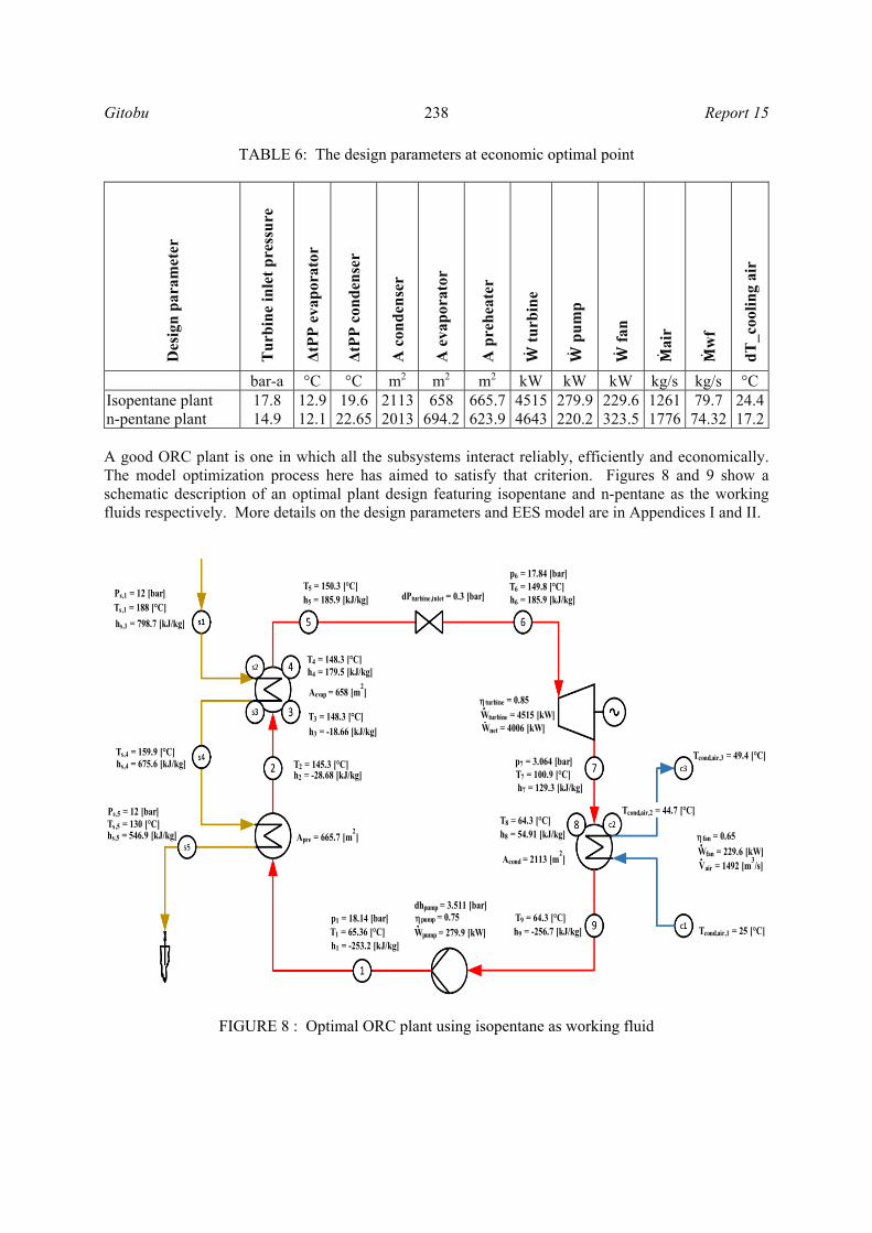
bar-a °C °C m2 m2 m2 kW kW kW kg/s kg/s °C Isopentane plant 17.8 12.9 19.6 2113 658 665.7 4515 279.9 229.6 1261 79.7 24.4n-pentane plant 14.9 12.1 22.65 2013 694.2 623.9 4643 220.2 323.5 1776 74.32 17.2 A good ORC plant is one in which all the subsystems interact reliably, efficiently and economically. The model optimization process here has aimed to satisfy that criterion. Figures 8 and 9 show a schematic description of an optimal plant design featuring isopentane and n-pentane as the working fluids respectively. More details on the design parameters and EES model are in Appendices I and II.

FIGURE 8 : Optimal ORC plant using isopentane as working fluid

Wpump = 279.9 [kW]

Wnet = 4006 [kW]

Wfan = 229.6 [kW]

dPturbine,inlet = 0.3 [bar]

fan = 0.65

pump = 0.75

turbine = 0.85

h1 = -253.2 [kJ/kg]

dhpump = 3.511 [bar]

h2 = -28.68 [kJ/kg]

h5 = 185.9 [kJ/kg] h6 = 185.9 [kJ/kg]

h7 = 129.3 [kJ/kg]

h9 = -256.7 [kJ/kg]

hs,1 = 798.7 [kJ/kg]

hs,4 = 675.6 [kJ/kg]

hs,5 = 546.9 [kJ/kg]

Ts,1 = 188 [°C]

Ts,4 = 159.9 [°C]

Ts,5 = 130 [°C]

T1 = 65.36 [°C]

T2 = 145.3 [°C]

T3 = 148.3 [°C]

T4 = 148.3 [°C]

T5 = 150.3 [°C] T6 = 149.8 [°C]

T7 = 100.9 [°C]

T8 = 64.3 [°C]

T9 = 64.3 [°C]

h3 = -18.66 [kJ/kg]

h4 = 179.5 [kJ/kg]

h8 = 54.91 [kJ/kg]

Vair = 1492 [m3/s]

Tcond,air,1 = 25 [°C]

Tcond,air,2 = 44.7 [°C]

Tcond,air,3 = 49.4 [°C]

Wturbine = 4515 [kW]

Acond = 2113 [m2]

Aevap = 658 [m2]

Apre = 665.7 [m2]

p1 = 18.14 [bar]

p6 = 17.84 [bar]

p7 = 3.064 [bar]

Ps,1 = 12 [bar]

Ps,5 = 12 [bar]


FIGURE 9 : Optimal ORC plant using n-pentane as working fluid 6. FINANCIAL ANALYSIS An optimized EES model provides the required sizes of major components like feed pump, preheater, evaporator, turbine and condenser. From their sizes one can estimate their costs. A rule of thumb is that the cost of these major components account for 50% of the plant cost. As explained earlier the other cost factors are the control system, SCADA system, back up installation, firefighting and other plant accessories. Then there is also some additional cost of civil works, power evacuation and environmental rehabilitation. The complete cost of implementing an optimal ORC plant using isopentane or n-pentane would then add up as shown in Table 7 below. 6.1 Effect of choice of the pinch points on the project cost and net turbine output Variation of flexible parameters has an effect on the plant performance and cost. In the design of the cooling system it needs to be considered that low condensation temperatures which lead to a higher output can only be achieved with high fan power and/or large cooling system sizes (Frick et al., 2015). The ΔtPP evap and ΔtPP_cond is linked to their sizes, cost and overall plant performance. A small pinch increases the performance of the evaporator but it is costlier because it requires a larger heat transfer area. A large pinch corresponds to a smaller and less costly evaporator and condenser but with reduced thermal performance. Figures 11 and 12 illustrate how deviation from the optimal pinch points affects the size and cost of these components for a plant running on n-pentane working fluid. A similar behaviour would be expected for the isopentane plant as well.

Wpump = 220.2 [kW]

Wnet = 4100 [kW]

Wfan = 323.5 [kW]

dPturbine,inlet = 0.3 [bar]

fan = 0.65

pump = 0.75

turbine = 0.85

h1 = 89.27 [kJ/kg]

dhpump = 2.963 [bar]

h2 = 317 [kJ/kg]

h5 = 559.9 [kJ/kg] h6 = 559.9 [kJ/kg]

h7 = 497.4 [kJ/kg]

h9 = 86.31 [kJ/kg]

hs,1 = 798.7 [kJ/kg]

hs,4 = 668.8 [kJ/kg]

hs,5 = 547 [kJ/kg]

Ts,1 = 188 [°C]

Ts,4 = 158.3 [°C]

Ts,5 = 130 [°C]

T1 = 62.56 [°C]

T2 = 144.4 [°C]

T3 = 147.4 [°C]

T4 = 147.4 [°C]

T5 = 149.4 [°C] T6 = 148.9 [°C]

T7 = 99.77 [°C]

T8 = 61.7 [°C]

T9 = 61.7 [°C]

h3 = 326.7 [kJ/kg]

h4 = 554.3 [kJ/kg]

h8 = 422 [kJ/kg]

Vair = 2103 [m3/s]

Tcond,air,1 = 25 [°C]

Tcond,air,2 = 39.05 [°C]

Tcond,air,3 = 42.2 [°C]

Wturbine = 4643 [kW]

Acond = 2013 [m2]

Aevap = 694.3 [m2]

Apre = 624 [m2]

p1 = 15.2 [bar]

p6 = 14.9 [bar]

p7 = 2.254 [bar]

Ps,5 = 12 [bar]

Ps,1 = 12 [bar]


TABLE 7: Summary cost of a plant using either isopentane or n-pentane

Component Isopentane n-pentane

SizeCost

(USD) Size

Cost (USD)

Preheater(m2) 665.7 332,855.00 623.9 311,965.00Evaporator (m2) 658 296,099.00 694.2 312,404.00Turbine (kW) 4515 2,032,000.00 4643 2,089,000.00Condenser (m2) 2113 1,268,000.00 2013 1,208,000.00Feed pump (kW) 279.9 125,937.00 220.2 99,103.00Cooling tower fan motor (kW) cost included in the condensor 229.6 323.5 Plant cost related to controls, SCADA and backup installations

4,054,891.00 4,020,472.00

Civil, mechanical, evacuation and environmental costs from Table 5

984,300.00 984,300.00

Total cost of the plant (USD) 9,094,082.00 9,025,244.00Net power from the plant (kW) 4006 4099 Specific cost of the plant (Plant cost/netpower) USD/kW 2,270.10 2,201.80 The optimal pinches for the evaporator and condenser may seem large, but the reason for this is that the cost of the wells and the supply system is already apportioned to the existing flash plant. The effect of this is that the optimum pinch for the evaporator and condenser shifts upward from what is expected in a plant with high upfront cost. 7. CONCLUSIONS This paper has looked at the details of generating additional power using combined brine stream from separator stations SD2 and SD3 in Olkaria Domes field. The mode of power generation examined here is the ORC plants which is a widely tested and proven technology operating reliably in many countries. Isopentane and n-pentane have been found appropriate for use as working fluids but there is a slight economic advantage in using the latter. One unique advantage of installing bottoming ORC plants in a developed field like Olkaria is that most of the major upfront costs like the field exploration and drilling, steam field systems and road networks are already assigned to the conventional power plants. The key cost associated with an ORC plant would be the cost of the plant

2500

3000

3500

4000

4500

5000

5500

6000

0 5 10 15 20 25 30 35

Net

turb

ine

outp

ut (

kW)

ΔtPP (°C)

ΔtPP cond vs net plant output ΔtPP vap vs plant specific costFIGURE 10: Variation of net power against ΔtPP

2150

2200

2250

2300

2350

2400

2450

2500

2550

2600

2650

0 5 10 15 20 25 30 35

Z_s

pec

(USD

/kW

)

ΔtPP (°C)

ΔtPP cond vs plant specific cost ΔtPP vap vs plant specific cost

FIGURE 11: Variation of plant cost against ΔtPP


itself which is normally delivered as a modular unit on an EPC contract basis. The other costs are minimal like civil, mechanical, electrical and environmental costs. Thus, this paper concludes and recommends that installation of an ORC plant on this brine stream is viable and a quick win for the company.

ACKNOWLEDGEMENTS First and foremost, I want to pay my gratitude to my employer Kenya Electricity Generating Company (KenGen) and the United Nations University Geothermal Training Program (UNU-GTP) for granting me the chance to attend this course. I cannot describe adequately the unwavering support I got from Mr. Lúdvík S. Georgsson, Mr. Ingimar G. Haraldsson, Mr. Markús A.G. Wilde, Ms. Thórhildur Ísberg and Ms. Málfrídur Ómarsdóttir but I will forever be grateful. I did this project under supervision of Dr. Páll Valdimarsson. He was a good teacher to me and I could always count on him when stuck. The research and compilation of this project report has taken a lot of advantage of his wealth of experience in ORC power plants. I also want to acknowledge that I was immensely privileged to be with the UNU-GTP group of 2016 and we had a lot in common. I will specifically carry home the memories of the football we played, the mountains we hiked and the jogging we did together. Zsófia Unyi and Adrian Foghis, you have my best regards for inspiring me to run the Reykjavik Marathon. Finally a special thanks goes to my family who kept on checking on me regularly and ultimately honor and glory belongs to God for strengthening and protecting me all the time.

NOMENCLATURE A = Area (m2) cond = Condensor dT_C = Cooling air temperature difference at inlet and outlet of the condenser (°C) evap = Evaporator EES = Engineering Equation Solver h = Enthalpy (kJ/kg) KenGen = Kenya Electricity Generating Company LTD kV = Kilovolts kW = Kilowatts LMTD = Log mean temperature difference (°C)

= Mass flow rate (kg/s) ORC = Organic Rankine cycle P = Pressure (bar_a) Pre = Preheater S = Entropy (kJ/kgK) T = Temperature (°C) Turb = Turbine Turb ip = Turbine inlet pressure

= Volumetric flow rate (m3/S) = Power (kW)

West Jec = West Japan Engineering Consultants Inc wf = Working fluid ΔtPP = Pinch point temperature difference (°C)

= Efficiency


REFERENCES

Chen, H., Goswami, D.Y., and Stefanakos, E.K., 2010: A review of thermodynamic cycles and working fluids for the conversion of low grade heat. Renewable & Sustainable Energy Reviews, 14, 3059-3067. DiPippo, R., 2007: Geothermal power plants. Principles, applications, case studies and environmental impact (2nd ed.). Butterworth Heineman, Elsevier, Kidlington, United Kingdom, 493 pp. Eastop, T.D., and MacConkey, A., 1993: Applied thermodynamics for engineering technologist. Longman, England, United Kingdom, 715 pp. Frick, S., Saadat, A., Surana, T., Siahaan, E.E., Kupfermann, G.A., Erbas, K., Huenges, E., Gani, M.A., 2015: Geothermal binary power plant for Lahendong, Indonesia: A German-Indonesian collaboration project. Proceedings of the World Geothermal Congress 2015, Melbourne, Australia, 5 pp. Habibzadeh, A., and Rahsid, M.M., 2016: Thermodynamic analysis of different working fluids used in organic Rankine cycle for recovering waste heat from GT-MHR. J. Eng. Science and Technology, 11-1, 121-135. KenGen, 2014: Feasibility study for geothermal power generation for brine at Olkaria. West Jec report for Kenya Electricity Generating Company Ltd., unpublished internal report. KenGen, 2016: Final report of the 3rd Board of Consultants. Kenya Electricity Generating Company Ltd., unpublished report. Kopunicova, M., 2009: Feasibility study of binary geothermal power plants in Eastern Slovakia - Analysis of ORC and Kalina power plants. University of Iceland and University of Akureyri, The School of Renewable Energy Science, MSc thesis, 73 pp. Monroy Parada, A.F., 2013: Geothermal binary cycle power plant principles, operation and maintenance. Report 15 in: Geothermal training in Iceland 2013. United Nations University Geothermal Training Programme, Iceland, 443-476. Valdimarsson, P., 2011: Geothermal power plant cycles and main components. Paper presented at “Short Course on Geothermal Drilling, Resource Development and Power Plants”, organized by UNU-GTP and LaGeo, in Santa Tecla, El Salvador, 24 pp. Wikipedia, 2016a: Logarithmic mean temperature difference. Wikipedia, website: en.wikipedia.org/wiki/Logarithmic_mean_temperature_difference. Wikipedia, 2016b: List of refrigerants. Wikipedia, website: en.wikipedia.org/wiki/List_of_refrigerants. Wolverine, 2016: Heat transfer to air-cooled heat exchangers. Wolverine Tube Inc., website: www.wlv.com/wp-content/uploads/2014/06/data/db3ch6.pdf.


APPENDIX I: Detailed thermodynamic cycle state points

Isopentane plant cycle details Power conversion cycle Geothermal fluid (brine) cycle Cooling system cycle

State point

h T p v s State point

P T h Q State point

T Q [kJ/kg] [°C] [bar] [m^3/kg] kj/kgK [bar] [°C] [kJ/kg] kJ/s [°C] kJ/s

1 -253.2 65.36 18.14 0.001741 -1.395 S1 12 188 798.7 0 C1 25 0 2 -28.68 145.3 18.14 0.002187 -0.802 S2 12 187.2 795 17893 C2 44.7 248363 -18.66 148.3 18.14 0.002221 -0.778 S3 12 161.2 681.3 18692 C3 49.4 307664 179.5 148.3 18.14 0.01746 -0.308 S4 12 159.9 675.6 34486 5 185.9 150.3 18.14 0.01784 S5 12 130 546.9 35001 6 185.9 149.8 17.84 0.01829 -0.292 7 129.3 100.9 3.064 0.1315 -0.265 8 54.91 64.3 3.064 0.1145 -0.474 9 -256.7 64.3 3.064 0.001747 -1.397

n-pentane cycle details

Power conversion cycle Geothermal fluid (brine) cycle Cooling system cycleState point

h T p v s State point

P T h Q State point

T Q [kJ/kg] [°C] [bar] [m^3/kg] kj/kgK [bar] [°C] [kJ/kg] kJ/s [°C] [kJ/s]

1 89.27 62.56 15.2 0.001712 0.275 S1 12 188 798.7 0 C1 25 0 2 317 144.4 15.2 0.002123 0.879 S2 12 187.3 795.7 16927 C2 39.05 249523 326.7 147.4 15.2 0.002151 0.902 S3 12 159.5 674 17644 C3 42.2 305564 554.3 147.4 15.2 0.0223 1.444 S4 12 158.3 668.8 34565 5 559.9 149.4 15.2 0.02266 S5 12 130 547 34980 6 559.9 148.9 14.9 0.0233 1.459 7 497.4 99.77 2.254 0.1807 1.488 8 422 61.7 2.254 0.158 1.275 9 86.31 61.7 2.254 0.001716 0.273

APPENDIX II: EES code {Fluid$ = 'Isobutane'} {Fluid$ = 'n-butane'} Fluid$ = 'Isopentane' {Fluid$ = 'n-pentane'} { Fluid$ = 'R245fa'} T_air = 25 {P_turbine_inlet = 14.91} dP_turbine_inlet = 0.3 eta_pump = 0.75 T_boiling_margin = 3 T_superheat = 2 eta_turbine = 0.85 T_source_in = 188 P_source_in = 12 m_dot_source = 139 Cp_air = 1.00 {T_pinch_vap = 12.2} {T_pinch_cond_fake = 18.75} {dT_c = 17.27} T_air_out = T_air + dT_c

T_condensation = T_air_out + T_pinch_cond_fake s_in = 1 s_dew = 2 s_bubble = 3 s_vap_out = 4 s_pre_in = 4 s_pre_out = 5 s_plant_out =5 pump_out = 1 pre_in = 1 pre_out = 2 vap_in = 2 vap_bubble = 3 vap_dew = 4 vap_out = 5 turb_in = 6 turb_out = 7 cond_in = 7 cond_dew = 8 cond_out = 9 pump_in = 9


p_vap = 450 p_pre = 500 p_cond = 600 p_turb = 450 p_pump = 450 {Pump inlet - condenser hot well} T[pump_in] = T_condensation h[pump_in] = enthalpy(Fluid$, T=T[pump_in], x=0) p[pump_in] = pressure(Fluid$, T=T[pump_in], x=0) v[pump_in] = volume(Fluid$, T=T[pump_in], x=0) {System pressures} p[cond_dew] = p[cond_out] p[cond_in] = p[cond_dew] p[turb_in] = P_turbine_inlet p[vap_out] =p[turb_in] + dP_turbine_inlet p[vap_dew] = p[vap_out] p[vap_bubble] = p[vap_dew] p[vap_in] = p[vap_bubble] p[pre_in] = p[pre_out] {Pump outlet} dh_pump = v[pump_in]*(p[pump_out]- p[pump_in])*100/eta_pump h[pump_out] = h[pump_in] + dh_pump T[pump_out] = temperature(Fluid$, P=p[pump_out], h=h[pump_out]) s[pump_out] = entropy(Fluid$, P=p[pump_out], h=h[pump_out]) v[pump_out] = volume(Fluid$, P=p[pump_out], h=h[pump_out]) {Preheater outlet} T[pre_out] = temperature(Fluid$, p= p[pre_out], x=0) - T_boiling_margin h[pre_out] = enthalpy( Fluid$, p= p[pre_out],T=T[pre_out]) s[pre_out] = entropy( Fluid$, p= p[pre_out],T=T[pre_out]) v[pre_out] = volume( Fluid$, p= p[pre_out],T=T[pre_out]) {Vaporizer bubble point} h[vap_bubble] = enthalpy(Fluid$, p= p[vap_bubble], x=0) T[vap_bubble] = temperature(Fluid$, p= p[vap_bubble], x=0) s[vap_bubble] = entropy(Fluid$, p= p[vap_bubble], x=0) v[vap_bubble] = volume(Fluid$, p= p[vap_bubble], x=0)

{Vaporizer dew point} h[vap_dew] = enthalpy(Fluid$, p= p[vap_dew], x=1) T[vap_dew] = temperature(Fluid$, p= p[vap_dew], x=1) s[vap_dew] = entropy(Fluid$, p= p[vap_dew], x=1) v[vap_dew] = volume(Fluid$, p= p[vap_dew], x=1) {Vaporizer Outlet} T[vap_out] = T[vap_dew] + T_superheat h[vap_out] = enthalpy(Fluid$, p= p[vap_out], T=T[vap_out]) v[vap_out] = volume(Fluid$, p= p[vap_out], T=T[vap_out]) {Turbine inlet} h[turb_in] = h[vap_out] T[turb_in] = temperature(Fluid$, p= p[turb_in], h=h[turb_in]) s[turb_in] = entropy(Fluid$, p= p[turb_in], h=h[turb_in]) v[turb_in] = volume(Fluid$, p= p[turb_in], h=h[turb_in]) {Turbine outlet} h_s_turb_out = enthalpy(Fluid$, p= p[turb_out], s=s[turb_in]) h[turb_out] = h[turb_in] - (h[turb_in] - h_s_turb_out)*eta_turbine T[turb_out] = temperature(Fluid$, p= p[turb_out], h=h[turb_out]) s[turb_out] = entropy(Fluid$, p= p[turb_out], h=h[turb_out]) v[turb_out] = volume(Fluid$, p= p[turb_out], h=h[turb_out]) {Condenser due point} h[cond_dew] = enthalpy(Fluid$, p= p[cond_dew], x=1) T[cond_dew] = temperature(Fluid$, p= p[cond_dew], x=1) s[cond_dew] = entropy(Fluid$, p= p[cond_dew], x=1) v[cond_dew] = volume(Fluid$, p= p[cond_dew], x=1) {Condenser outlet} {h[cond_out] = enthalpy(Fluid$, p= p[cond_dew], x=0)} {T[cond_out] = enthalpy(Fluid$, p= p[cond_dew], x=0)} s[cond_out] = entropy(Fluid$, p= p[cond_dew], x=0) {v[cond_out] = volume(Fluid$, p= p[cond_dew], x=0) } {Source fluid pressure} P_s[s_in] = P_source_in


P_s[s_dew] = P_s[s_in] P_s[s_bubble] = P_s[s_dew] P_s[s_vap_out] = P_s[s_bubble] P_s[s_pre_out] = P_s[s_pre_in] {Mass flow calculation} {T_s[s_in] = T_source_in} T_s[s_in] = temperature(Water, P=P_s[s_in], x = 0) h_s[s_in] = enthalpy(Water, P=P_s[s_in], x = 0) T_s[s_bubble] = T[vap_bubble] + T_pinch_vap h_s[s_bubble] = enthalpy(Water, P=P_s[s_in], T=T_s[s_bubble]) Q_dot_rhs = m_dot_source*(h_s[s_in] - h_s[s_bubble]) m_dot_wf = Q_dot_rhs /(h[vap_out]-h[vap_bubble]) Q_dot_superheat = m_dot_wf *(h[vap_out] - h[vap_dew]) h_s[s_dew] = h_s[s_in] - Q_dot_superheat /m_dot_source T_s[s_dew] = temperature(Water, h= h_s[s_dew] , P=P_s[s_dew]) Q_dot_pre_vap = m_dot_wf * (h[vap_bubble] - h[pre_out]) h_s[s_vap_out] = h_s[s_bubble] - Q_dot_pre_vap/ m_dot_source T_s[s_vap_out] = temperature(Water, h= h_s[s_vap_out] , P=P_s[s_vap_out]) Q_dot_preheater = m_dot_wf *(h[pre_out]-h[pre_in]) h_s[s_Pre_out] = h_s[s_Pre_in] - Q_dot_preheater/m_dot_source T_s[s_Pre_out] = temperature(Water, P=P_s[s_pre_out] , h=h_s[s_Pre_out]) W_dot_turbine = m_dot_wf * (h[turb_in]-h[turb_out]) W_dot_pump = m_dot_wf * (h[pump_out]-h[pump_in]) W_dot_net = W_dot_turbine - W_dot_pump - Work_dot_fan {T-q modelling} {Preheater} {Point 1 - pump outlet/preheater inlet} Q_dot[1] = 0 T_cold[1] = T[pump_out] T_hot[1] = T_s[s_Pre_out] {Point 2 preheater outlet / vapourizer inlet} Q_dot[2] = Q_dot[1] + Q_dot_preheater T_cold[2] = T[pre_out] T_hot[2] = T_s[s_vap_out]

{Point 3 - vaporizer bubble point} Q_dot[3] = Q_dot[2] + Q_dot_pre_vap T_cold[3] = T[vap_bubble] T_hot[3] = T_s[s_bubble] {Point 4 - vaporizer dew point} Q_dot[4] = Q_dot[3] +(Q_dot_rhs - Q_dot_superheat) T_cold[4] = T[vap_dew] T_hot[4] = T_s[s_dew] {Point 5 - vaporizer outlet} Q_dot[5] = Q_dot[4] + Q_dot_superheat T_cold[5] = T[vap_out] T_hot[5] = T_s[s_in] {Condensor heat exchanger model} Q_turbin_turbout = m_dot_wf * (h[turb_in]-h[turb_out]) Q_turbout_conddew = m_dot_wf * (h[turb_out] - h[cond_dew] ) Q_conddew_condout = m_dot_wf * ( h[cond_dew] - h[pump_in] ) {T-q model for condensor} {Condensor inlet} Q_cond[1] = 0 {Q_dot[5] - Q_turbin_turbout} T_cond_w[3] = t[turb_out] T_cond_air[1] = T_air {Condensor dewpoint} Q_cond[2] =Q_conddew_condout {Q_cond[1] - Q_turbout_conddew } T_cond_w[2] = T[cond_dew] {Condensor outlet} {Pinch point of 5deg C assumed at condensor outlet} Q_cond[3] = {Q_cond[2] - Q_conddew_condout }Q_turbout_conddew +Q_conddew_condout T_cond_w[1] = T[pump_in] T_cond_air[3] = {T[pump_in] - T_pinch_cond_fake} T_air_out {Mass flow of air needed and T_air_dew analysis} M_cond_air * Cp_air * (T_cond_air[3] - T_cond_air[2]) = {Q_conddew_condout }Q_turbout_conddew M_cond_air * Cp_air * (T_cond_air[2] - T_air) = {Q_turbout_conddew}Q_conddew_condout V_dot_air = M_cond_air * density(Air, T=T_air, P=1.013) {Heat exchanger area analysis} {Preheater exchange area analysis} LMTD_pre = ((T_s[s_vap_out] - T[pre_out]) - (T_s[s_Pre_out] - T[pump_out])) /


ln((T_s[s_vap_out] - T[pre_out]) / (T_s[s_Pre_out] - T[pump_out])) U_pre = 0.8 A_pre = Q_dot_preheater/(U_pre * LMTD_pre) {Evaporator exchange analysis} {Area required to heat fluid up to boiling point} LMTD_Preout_vapbubble = ((T_s[s_bubble] - T[vap_bubble]) - (T_s[s_vap_out] - T[pre_out])) / ln((T_s[s_bubble] - T[vap_bubble]) / (T_s[s_vap_out] - T[pre_out])) U_preout_vapbubble = 0.8 A_preout_vapbubble = Q_dot_pre_vap/(U_preout_vapbubble * LMTD_Preout_vapbubble) {Area required to heat fluid up to vapour saturation point} LMTD_vapbubble_vapdew = ((T_s[s_dew] - T[vap_dew]) - (T_s[s_bubble] - T[vap_bubble])) / ln((T_s[s_dew] - T[vap_dew]) / (T_s[s_bubble] - T[vap_bubble])) U_vapbubble_vapdew = 1.2 A_vapbubble_vapdew = (Q_dot_rhs - Q_dot_superheat)/(U_vapbubble_vapdew * LMTD_vapbubble_vapdew) {Area required to superheat the fluid to 2deg C} LMTD_vapdew_vapsheat = ((T_s[s_in] - T_s[s_vap_out]) - (T_s[s_dew] - T[vap_dew])) / ln((T_s[s_in] - T_s[s_vap_out]) / (T_s[s_dew] - T[vap_dew])) U_vapdew_superheat = 0.6 A_vapdew_superheat = Q_dot_superheat/(U_vapdew_superheat*LMTD_vapdew_vapsheat) {Air cooled condenser area required} {Area required to bring turbine exhaust vapour to dewpoint} LMTD_turbout_conddew = (( t[turb_out] - T_cond_air[3]) - (T[cond_dew] - T_cond_air[2])) / ln(( t[turb_out] - T_cond_air[3]) / (T[cond_dew] - T_cond_air[2])) U_turbout_conddew= 0.5 A_turbout_conddew = Q_turbout_conddew/(U_turbout_conddew*LMTD_turbout_conddew)

{Area required to cool fluid from dewpoint to liquid saturation (pump inlet) point} LMTD_conddew_condout = (( T[cond_dew] - T_cond_air[2]) - (T[pump_in] - T_cond_air[1])) / ln((T[cond_dew] - T_cond_air[2]) / (T[pump_in] - T_cond_air[1])) U_conddew_condout= 0.5 A_conddew_condout= Q_conddew_condout/(U_conddew_condout*LMTD_conddew_condout) {Total evaporator area required} A_evap = ((A_preout_vapbubble)+(A_vapbubble_vapdew)+(A_vapdew_superheat)) {Total condensor area required} A_cond = ((A_turbout_conddew)+(A_conddew_condout)) T_pinch_cond_calc = T_cond_w[2] - T_cond_air[2] {Fan power} dP_cond_air = 0.001 eta_fan = 0.65 Work_dot_fan = (V_dot_air * dP_cond_air *100)/eta_fan Z_vap = p_vap * A_evap Z_pre = p_pre * A_pre Z_cond = p_cond * A_cond Z_turb = p_turb * W_dot_turbine Z_pump = p_pump * W_dot_pump Z_mc = Z_vap + Z_pre + Z_cond + Z_turb + Z_pump {Z_plant = 5000000} Z_plant = Z_mc Z_source = 984300 Z_total = Z_mc + Z_plant + Z_source z_spec_mc =Z_mc / W_dot_net z_spec =Z_total / W_dot_net P_vap_junk = P_turbine_inlet * 130/T_s[5]

Documents

MODEL ORGANIC RANKINE CYCLE FOR BRINE AT … ORGANIC RANKINE CYCLE FOR BRINE AT OLKARIA GEOTHERMAL FIELD, KENYA ... An internal report from KenGen’s ... the pump outlet assuming