Model order reduction for nonlinear IC models.

A. Verhoeven12, J. ter Maten12, M. Striebel13, and R. Mattheij2

1 NXP Semiconductors (Design Methods) jan.ter.maten@nxp.com2 Eindhoven University of Technology (CASA) Arie.Verhoeven@na-net.ornl.gov3 Chemnitz University of Technology michael.striebel@nxp.com

Summary. In this paper we demonstrate model order reduction for a nonlinearacademic model of a diode chain. Two reduction methods, which are suitable fornonlinear differential algebraic equation systems are used, the Trajectory PieceWiseLinear approach and the Proper Orthogonal Decomposition with Missing Point Es-timation.

1 Introduction

The dynamics of electrical circuits at time t can be generally described bythe nonlinear, first order, differential-algebraic equation (DAE) system of theform:

ddt [q(x)] + j(x) + Bu = 0, x(0) = x0,

y = h(x),, (1)

where x : R → Rd represents the unknown vector of circuit variables in timet, the vector-valued functions q, j : R× Rd → Rd represent the contributionsof, respectively, reactive elements (such as capacitors and inductors) and ofnonreactive elements (such as resistors) and B ∈ Rd×m is the distributionmatrix for the excitation vector u : R → Rm that controls the output re-sponse y : R → Rp. We assume that d m, p. There are several establishedmethods, such as sparse-tableau, modified nodal analysis, etc. which generatethe system (1) from the netlist description of electrical circuit. The dimensiond of the unknown vector x is of the order of the number of elements in thecircuit, which means that it can be extremely large, as today’s VLSI circuitshave hundreds of millions of elements.Mathematical model order reduction (MOR) aims to replace the originalmodel (1) by a system of much smaller dimension, which can be solved bysuitable DAE solvers within acceptable time. Because we are only interestedin the relationship between u and y in the time-domain, the model can bereplaced by a low-order model for z : R → Rr, like

2 Arie Verhoeven et alddt [q(z)] + j(z) + Bu = 0, z(0) = z0,

y = h(z).(2)

At present, however, only linear MOR techniques are well-enough developedand properly understood to be employed [1]. To that end, we either linearisethe system (1) or decouple it into nonlinear and linear subcircuits (intercon-nect macromodeling of parasitic subcircuits [8]). For dynamical systems theobservability and controllability functions [1] are defined by

Lc(x0) = min12

∫ 0

−∞‖u(t)‖2dt : u ∈ L2(−∞, 0),x(−∞) = 0,x(0) = x0,

Lo(x0) =12

∫ ∞

0

‖y(t)‖2dt,∀τ∈[0,∞)u(τ) = 0,x(0) = x0.

They represent the minimum amount of input energy to reach state x0 andthe output energy that comes free when starting at state x0. (cp. kinetic andpotential energy in mechanical systems). The system is in balanced form atbasis V if the (energy) ratio Lo(Vz)

Lc(Vz)is balanced. For linear time-invariant

(LTI) systems as x = Ax + Bu, x(0) = x0,

y = Cx,(3)

we have Lc(x0) = 12x

T0 W−1x0 and Lo(x0) = 1

2xT0 Mx0, where W,M ∈ Rd×d

are the controllability and observability Gramians, which are symmetric pos-itive definite matrices. They satisfy the well-known Lyapunov equations

AW + WAT = −BBT , (4)AT M + MA = −CT C. (5)

An LTI system is balanced w.r.t. basis V if W = VΣVT and M = V−T ΣV−1

are simultaneously diagonalised, such that

Lo(x)Lc(x)

=xT Mx

xT W−1x=

xT V−T ΣV−1xxT V−1Σ−1V−T x

=zT Σ2zzT z

.

For redundant systems the singular values of Σ converge rapidly to zero. Thisallows to obtain an accurate reduced model by Truncated Balanced Realisa-tion (TBR). There also exist many other much cheaper MOR techniques forLTI systems, like PRIMA, PVL, PMTBR, SPRIM, etc. For the special caseA = AT ,B = CT it follows from (4),(5) that W = M. Then it is possible tofind an orthogonal V such that W = M = VΣVT are balanced.For nonlinear systems as (1) it is no longer possible to apply these linear MORtechniques. Then we try to exploit the (piecewise) linear structure as well aspossible. The reduced model can be constructed for a benchmark simulation,such that it is accurate if the solution is in the neighbourhood of the bench-mark solution. In this paper we present the application of some promising

MOR for nonlinear IC models 3

nonlinear reduction methods on some electronic circuit models. These are theTrajectory PieceWise Linear approach (TPWL) [12] and the Proper Orthog-onal Decomposition (POD) [2] supported by the Missing Point Estimation(MPE) technique [5].

2 Model order reduction for subcircuits

A continuously increasing number of functions is combined in each single inte-grated circuit. Therefore, complex devices are designed in a modular manner.Functional units like e.g., decoders, mixers, and operational amplifiers, aredeveloped by different experts and stored in device libraries. Other circuitdesigners then choose these models according to their requirements and in-stantiate them in higher level circuits. To enable the combination of differentblocks, each model is equipped with its own number of junctions, or pins, bywhich a communication with the outside world is possible.In the first instance, numerical simulations are run to verify a design. Hence, itis desirable to have, besides the exact circuit schematic, a suitable descriptionof the individual model that enables fast simulations, i.e., a library of reducedsubcircuit models.In circuits that are developed to act as a subcircuit in higher hierarchies asubset of its nodes are terminals. To this nodes both known inner elements aswell as elements whose nature may change with different instantiations of themodel are connected. Due to Kirchhoff’s current law, the sum of all currentsflowing into each single node is zero at each timepoint. In terms of the networkequations (1) the contribution of currents from inner elements at the termi-nals is covered by d

dtq(x) and j(x), respectively. As the nature, i.e. reactive ornonreactive, of the adjacent elements in the final circuit is not known, whenthe cell is designed, additional unknowns jpin, i.e. pin currents, are introducedon the subcircuit level. We assume that the cell under consideration has de

nodes and dpin < de of them are terminals. Then we can extend (1) to

d

dt[q(x)] + j(x) + Bu(t) + Apinjpin = 0, (6)

with jpin ∈ Rdpin and where Apin ∈ 0, 1d×dpin with dpin rows containingexactly one non-zero element is an incidence matrix describing the topologicaldistribution of the pin.The pin currents jpin can be determined when there is an external circuitryavailable, completing the network equations. During the process of developingthe single cell a suitable test bench that emulates the typical environment thesubcircuit will operate in later has to be defined by the designer.Communication amongst electrical devices is done in terms of time varyingvoltages and currents. Regarding the cell (6) we can either inject the currentsjpin and get the voltage response at the terminals or supply the voltages at

4 Arie Verhoeven et al

the pins and receive the according currents. The state x comprises the nodevoltages and the currents through inductors and voltage sources. With thepin currents’ incidence matrix Apin we can access the node voltages at theterminals by

xpin = ATpin · x. (7)

Now, current injection means regarding jpin as inputs returning xpin as theoutput. Therefore, we can write

0 =d

dt[q(x)] + j(x) +

(B Apin

) (u(t)

jpin(t)

),

y = ATpinx.

Voltage injection on the other hand implies that the node voltages at theterminals are prescribed and corresponding pin currents are additional un-knowns, i.e., they are added to the state vector:

0 =d

dt

(q(x)0

)+

(j(x) + Apinjpin

−ATpinx

)+

(B

I

) (u(t)

xpin(t)

)y =

(0 I

) (x

jpin

)Finally, the common structure of both approaches is

0 =d

dt[qλ(xλ)] + jλ(xλ) +

(Bλ Cλ

) (uλ(t)upin,λ

), (8a)

yλ = CTλ xλ ∈ Rdpin,λ , (8b)

where we introduce λ as an identifier for the cell, taken from some set I ofindices. Viewed from the outside, the cell (8) appears just in terms of itsinput-output behaviour, i.e., given upin,λ ∈ Rdpin,λ it returns yλ.Now, we turn our attention to the circuitry a cell might be embedded in. Weassume that the state space of this circuit level has dimension d, i.e., it isdescribed by the states x ∈ Rd. Furthermore, we let this level consist of r ∈ Ninstantiations of cells, i.e., I = 1, 2, . . . , r, only. After due consideration wesee that this electrical system is described by

0 =∑λ∈I

ATλyλ, with Aλ ∈ 0, 1dpin,λ×d

where yλ is determined by (8) with upin,λ = Aλx for all λ ∈ I. (9)

As all the instantiated cells appear just in terms of their input-output be-haviour, we are free to reduce the order of single models (8) and use themagain on level (9). Furthermore, as subcircuits are regarded as special ele-ments, we can also include other elements on this level. Hence we can writein general form again

MOR for nonlinear IC models 5

d

dt[q(x)] + j(x) + Bu = 0, with x =

(xT ,yT

1 , . . . ,yTr

)T, (10)

which can be seen as a subcircuit on another level again. In this way, a hier-archical model order reduction would be possible.

3 Trajectory Piecewise Linear Model Order Reduction

The idea behind the Trajectory Piecewise Linear (TPWL) method is to lin-earise (1) several times along a given trajectory x(t) (corresponding to sometypical input u(t)) that satisfies

d

dt[q(x)] + j(x) + Bu = 0. (11)

Note that in [15] an alternative version of TPWL is described where the non-linear functions q(t,x), j(t,x) are linearised around the Linearisation Tuples(ti, x(ti)). Below the nonlinear system itself is linearised around the completetrajectory x(t). Furthermore we can use just Linearisation Points (LPs) x(ti)instead of Linearisation Tuples because the system in (1) does not depend ex-plicitly on t and behaves linearly with respect to u. Define y(t) = x(t)− x(t)and u(t) = u(t)− u(t). Linearising the nonlinear equation (1) gives us

d

dt[q(x)] + j(x) + Bu +

d

dt[C(x)y] + G(x)y + Bu = 0.

Because the trajectory x(t) satisfies (11) we obtain the following time-varyinglinear system for y

d

dt[C(x(t))y(t)] + G(x(t))y(t) + Bu(t) = 0. (12)

The main idea of TPWL is to approximate the time-varying Jacobian matricesC(x(t)),G(x(t)) by a weighted combination of piecewise constant matrices.Then a (finite) sequence of linearised local systems is used to create a globallyreduced subspace. The final TPWL model is constructed as a weighted sumof all locally linearised reduced systems. The disadvantage of standard lineari-sation methods is that they only deliver good results in the neighbourhood ofthe chosen linearisation point (LP) x(ti). To overcome this several linearisedmodels are created in TPWL. The LPs can be computed simultaneously withthe numerical time-integration of (11) for the trajectory x(t). This procedurecan be described by the following steps:

1. Set an absolute accuracy factor ε > 0, set i = 1.2. Linearise the system around xi = x(ti). This implies:

Ciy + Giy + Bu(t) = 0, (13)

with Ci = ∂∂xq(x)

∣∣xi

and Gi = ∂∂xj(x)

∣∣xi

, where xi stays for x(ti). SaveCi, and Gi.

6 Arie Verhoeven et al

−1 0 1 2 3 4−1

−0.5

0

0.5

1

1.5

2

2.5

3

x1

x 2

A

B

D

E

C

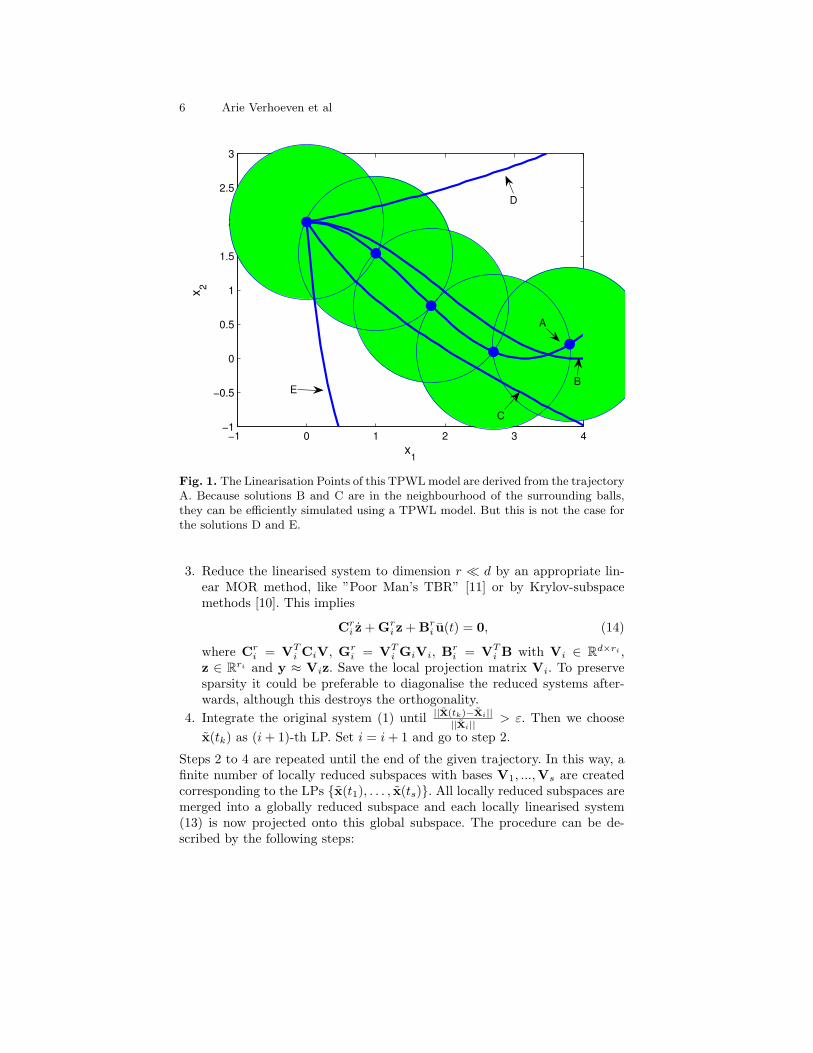
Fig. 1. The Linearisation Points of this TPWL model are derived from the trajectoryA. Because solutions B and C are in the neighbourhood of the surrounding balls,they can be efficiently simulated using a TPWL model. But this is not the case forthe solutions D and E.

3. Reduce the linearised system to dimension r d by an appropriate lin-ear MOR method, like ”Poor Man’s TBR” [11] or by Krylov-subspacemethods [10]. This implies

Cri z + Gr

i z + Bri u(t) = 0, (14)

where Cri = VT

i CiV, Gri = VT

i GiVi, Bri = VT

i B with Vi ∈ Rd×ri ,z ∈ Rri and y ≈ Viz. Save the local projection matrix Vi. To preservesparsity it could be preferable to diagonalise the reduced systems after-wards, although this destroys the orthogonality.

4. Integrate the original system (1) until ||x(tk)−xi||||xi||

> ε. Then we choosex(tk) as (i + 1)-th LP. Set i = i + 1 and go to step 2.

Steps 2 to 4 are repeated until the end of the given trajectory. In this way, afinite number of locally reduced subspaces with bases V1, ...,Vs are createdcorresponding to the LPs x(t1), . . . , x(ts). All locally reduced subspaces aremerged into a globally reduced subspace and each locally linearised system(13) is now projected onto this global subspace. The procedure can be de-scribed by the following steps:

MOR for nonlinear IC models 7

1. Define V = [V1, . . . ,Vs] ∈ Rd×(r1+...+rs).2. Calculate the SVD of V: V = UΣWT with U = [u1, . . . ,ud] ∈ Rd×d,Σ ∈

Rd×rs and W ∈ Rrs×rs, where r = (r1 + . . . + rs)/s.3. Define the new global projection matrix V ∈ Rd×r as [u1, . . . ,ur].4. Project each local linearised system (13) onto V.

Because of the construction of the global projection matrix V it is approxi-mately true that R(Vi) ⊂ R(V) for i = 1, . . . , s. All locally reduced linearisedreduced systems are combined in a weighted sum to build the global TPWLmodel. Note that the TPWL model in [15] directly approximates x instead ofy = x − x by Vz. Then it is necessary to add the defect of the trajectory xto the new input vector. But if the original state x = x + y is approximatedby x + Vz the reduced state z ∈ Rr satisfies

s∑i=1

wi(z)[VT CiVz + VT GiVz + VT Bu(t)

]= 0. (15)

In (15) we need weighting functions wi(z) that satisfy

s∑i=1

wi(z) = 1, wi(z) ∈ [0, 1].

The weighting function wi(z) determines the influence of the i-th local systemto the global system. Therefore it equals zero if z is far from the i-th projectedLinearisation Point VT x(ti). A very simple weighting function is defined by

wi(z) =

1 if i = minj | dj(z) = dmin(z),0 otherwise.

Here di(z) and dmin(z) are distance functions such that

di(z) = ‖z−VT x(ti)‖, i = 1, . . . , s,

dmin(z) = mindi(z), i = 1, . . . , s.

A more advanced alternative, with two free parameters α, ε > 0, can be usedlike

wi(z) =

exp(− αdi(z)

dmin(z) ) if exp(− αdi(z)dmin(z) ) > ε,

0 otherwise.

wi(z) =

[s∑

k=1

wk(z)

]−1

wi(z).

The TPWL method delivers reduced models that are cheap to simulate be-cause the reduced model (15) does not need any evaluations of the originalfunctions q, j and Jacobian matrices C,G, because all matrices VT CiV,VT GiV

8 Arie Verhoeven et al

and VT B can be computed before the simulation. The reduction error of aTPWL method consists of a linearisation and a truncation part. This errorcan be controlled by use of the Linearisation Points [15, 16]. Clearly the ac-curacy becomes higher for a large number of them. For strongly nonlinearsystems the price is that a large number of Linearisation Points is required tokeep the linearisation error sufficiently small. If the weighting functions wi(z)are not updated within the Newton method this will imply additional stepsizerestrictions.In the next three Sections we will show how nonlinear systems can be reducedwithout linearisation. then the reduced models are obtained by Galerkin pro-jection of the original model.

4 Empirical Balanced Truncation

For LTI sytstems the controllability and observability Gramians also satisfy

W =∫ ∞

0

eAtBBT eAT

tdt, M =∫ ∞

0

eAT

tCT CeAtdt. (16)

Consider X(t) = [x1, . . . ,xm] = eAtB and Y(t) = [y1, . . . ,yn] = CeAt. Letδ(t) be Dirac’s delta function, then xi and yj satisfy

d

dt[q(xi)] + j(xi) = biδ(t), xi(0) = 0, i = 1, . . . ,m, (17)ddt [q(xj)] + j(xj) = 0, xj(0) = ej ,

yj = h(xj),j = 1, . . . , n. (18)

Then it follows for LTI systems that the Gramians can be expressed in termsof the correlations of the states and outputs

W =∫ ∞

0

eAtBBT eAT

tdt =∫ ∞

0

X(t)X(t)T dt =m∑

i=1

∫ ∞

0

xi(t)xi(t)T dt,

and

M =∫ ∞

0

eAT

tCT CeAtdt =∫ ∞

0

Y(t)T Y(t)dt =n∑

i=1

∫ ∞

0

yi(t)T yi(t)dt.

If the states [x1, . . . ,xm] and [y1, . . . ,yn] are available, these Gramians W,Mcan be numerically integrated as follows

W ≈ W =m∑

i=1

1N

N∑k=1

xi(tk)xi(tk)T , M ≈ M =n∑

i=1

1N

N∑k=1

yi(tk)T yi(tk).

(19)

MOR for nonlinear IC models 9

For LTI systems we have that W → W, M → M if N → ∞. Empirical bal-anced truncation (EBT) applies these formulae for W, M to nonlinear systemswith a larger set of inputs and initial values to include also the nonlinear prop-erties. It is a powerful method because it really approximates the relationshipbetween the input and output and neglects all other phenomenons but alsoneeds a lot of experiments. Then TBR or another linear MOR technique isused to balance W, M by solving a system of Lyapunov equations. Thus abasis V can be constructed by truncation. The reduced model for z ∈ Rr isconstructed by Galerkin projection.

5 Proper Orthogonal Decomposition

The Proper Orthogonal Decomposition (POD), also known as the PrincipalComponent Analysis (PCA) and the Karhunen-Loeve expansion, is a specialcase of Empirical Balanced Truncation. It approximates the controllabilityGramian W by using only one trajectory.

W =1N

N∑k=1

x1(tk)x1(tk)T = VΣVT . (20)

Because the two Gramians are assumed to be equal, the POD basis can befound from the singular value decomposition

W = VΣVT ,

where V ∈ Rd×d is an orthogonal matrix and Σ a positive real diagonalmatrix.Thus the POD basis Vr =

(v1 . . . vr

)is an orthonormal basis and derived

from the collected state evolutions (snapshots)

X =(x(t1) . . . x(tN )

).

The POD method is particularly popular for systems governed by nonlinearpartial differential equations describing computational fluid dynamics. Ana-lytical solutions do not exist for such systems and the collected data may serveas the only adequate description of the system dynamics. The POD basis isfound by minimising the time-averaged approximation error given in (21)

av (‖ x(tk)− xn(tk) ‖2) . (21)

The averaging operator av(·) is defined as:

av(f) :=1N

N∑k=1

f(tk). (22)

10 Arie Verhoeven et al

Solving the minimisation problem of (21) is equivalent to computing the eigen-value decomposition of 1

N XXT . Because 1N XXT is a symmetric positive def-

inite matrix there exists an orthogonal matrix Vr ∈ Rd×r and a positive realdiagonal matrix Λr ∈ Rr×r such that

1N

XXT Vr = VrΛr. (23)

The term 1N XXT equals the state covariance matrix. The POD basis is a sub-

set of the eigenvectors of this covariance matrix and is stored by the matrixVr. The most important POD basis function is the eigenvector correspondingto the first eigenvalue. The truncation degree is determined from the eigen-value distribution in Λr = diag(λ1, . . . , λr). Based on the commonly adoptedad-hoc criterion, the truncation degree r should at least capture 99% of thetotal energy. The POD basis minimises, in Least Squares sense, (21) over allpossible bases. Error estimates for the solutions obtained from the reducedmodel are available in [9].

6 Galerkin projection

For each t let the state x(t) ∈ Rd belong to a separable Hilbert space X ,equiped with the Euclidian inner product. Then for all t the state x can beexpanded in a basis V =

(v1 . . . vd

)x(t) =

∑i∈I

zi(t)vi. (24)

The basis is derived from various criteria based on the approximation qualityof the original state x by its truncated expansion xr as defined in (25)

x(t) ≈ xr(t) =r∑

i=1

zi(t)vi. (25)

The order r of the truncated expansion is lower than the order d of the originalexpansion. Different reduction methods yield different basis.The reduced order model is the model that describes the dynamics of thebasis coefficients or the reduced state z = z1, . . . , zr. In many methodsthe reduced order model is derived by replacing the original state x by itstruncated expansion xr and projecting the original equations onto a truncatedbasis

Wr =(w1 . . . wr

).

Galerkin projection of (1) onto Vr along Wr results in the reduced DAEmodel

ddt

[WT

r q(Vrz)]

+ WTr j(Vrz) + WT

r Bu = 0, z(0) = z0,

y = h(Vrz).(26)

MOR for nonlinear IC models 11

The original d-dimensional DAE model is reduced to an r-dimensional DAEreduced order model by means of the Galerkin projection. Unfortunately, theresulting reduced order model (26) for z ∈ Rr is not always solvable for anyarbitrary truncation degree r. Furthermore in contrast to TPWL this reducedmodel still needs evaluations of the original model, because the functionsVT

r q(t,Vrz),VTr j(t,Vrz) can not be expanded before the simulation.

For circuit models the snapshots can be collected from a transient simulationwith fixed parameters and sources. The reduced model can also be used toapproximate the model for different parameters or sources as long as thesolution still approximately lies in the projected space. For circuit models witha lot of redundancy the reduced model can have a much smaller dimension.Unfortunately, direct application of POD to circuit models does not workwell in practice. Firstly, for Differential Algebraic Equations the Galerkinprojection scheme may yield an unsolvable reduced order model. This problemhas been studied in more detail in [5, 13]. Secondly, the computational effortrequired to solve the reduced order model and the original model is aboutthe same in nonlinear cases. This is due to the fact that the evaluation costsof the reduced model (26) are not reduced at all because Vr will be a densematrix in general.

7 Missing Point Estimation (MPE)

As mentioned before many MOR techniques for nonlinear systems as (1) useGalerkin projection to obtain a reduced model of the following type

d

dt

[WT q(Vz)

]+ WT j(Vz) + WT Bu = 0. (27)

The original state can be obtained by x = Vz. Thus indeed it is assumed thatx ∈ R(V). If x ∈ Rd and V ∈ Rd×r where r d it is clear that the reducedmodel (27) is of much smaller size than the original model (1). For LTI systemswith q(t,x) = Cx and j(t,x) = Gx − s(t) it is really possible to reduce thesimulation time for small r. In particular if the reduced model is diagonalised,we certainly get a model that is very cheap to solve. For the general case itis much worse because then the evaluation costs are not reduced at all. Butif the linear algebra part is dominant, we still can expect a speed-up. Despitethe resulting low dimensional model, the computational effort required tosolve the reduced order model and the original model is relatively the samein nonlinear cases. It may even occur that the original model is cheaper toevaluate than the reduced order model. The low dimensionality is obtainedby means of projection, either by the Galerkin projection method or the leastsquare method. In the projection schemes, the original numerical model mustbe projected onto the projection space. It implies that the original model mustbe re-evaluated when the original numerical model is time-varying, which isthe general case for nonlinear systems. A consequence is that the evaluation

12 Arie Verhoeven et al

costs for the reduced model are not reduced at all.Missing Point Estimation (MPE) is a well-known technique that modifies thematrix V such that only a part of the equations of the original model haveto be evaluated. This makes POD applicable for model order reduction ofnonlinear DAEs. The Missing Point Estimation (MPE) was proposed in [2]as a method to reduce the computational cost of reduced order, nonlinear,time-varying models. The method is inspired by the Gappy-POD approachthat was introduced by Everson and Sirovich in [7]. More details can be foundin [5, 14].

7.1 Adapted POD method

Assume that we have a benchmark solution x(t) of the DAE (1). Consider thesnapshot matrix X ∈ Rd×N . Consider the singular value decomposition of X:

X = UΣVT ,

where U ∈ Rd×d,V ∈ RN×N are orthogonal matrices and Σ ∈ Rd×N . Thusthe correlation matrix satisfies W = 1

N XXT = 1N UΣΣT UT . Because ΣΣT ∈

Rd×d is a positive real diagonal matrix we can write ΣΣT = Γ 2, where Γ ∈Rd×d is another positive real diagonal matrix.In contrast to POD we introduce the matrix L = UΓ ∈ Rd×d, such that alsoW = 1

N LLT . Note that the columns of L are still an orthogonal basis but notorthonormal. Then we transform the original system (1) by writing x = Lyand using orthogonal Galerkin projection as follows

d

dt

[LT q(Ly)

]+ LT j(Ly) + LT Bu = 0, x = Ly. (28)

Note that we are able to compute the matrix LT B before the simulation incontrast to the nonlinear functions LT q(Ly) and LT j(Ly). Therefore we aregoing to approximate LT and L such that LT q(Ly) and LT j(Ly) becomecheaper to evaluate. Note that we will use different approximations for Land LT . Because L = UΓ we can approximate it by UrΓrPr = LPT

r Pr

where Ur ∈ Rd×r and Γr ∈ Rr×r consists of the r most dominant singularvalues of Γ and Pr ∈ 0, 1r×d is a selection matrix. The matrices Ur, Γr andPr easily follows from the singular value decomposition. But if we use thisapproximation we still have the problem that for each function f the projectedfunction LT f ≈ PT

r ΓrUTr f still needs all elements of f . Therefore we use here

also another approximation

LT ≈ TgPg = LT PTg Pg, (29)

where Pg ∈ 0, 1g×d is another selection matrix and Tg ∈ Rd×g contains theg columns of LT with largest norm. If the singular values of Γ decrease rapidlywe often need just a small number g of columns. This means that the aliasing

MOR for nonlinear IC models 13

error ‖TgPg − LT ‖ also converges rapidly to zero. Now we can approximatethe transformed DAE (28) by

d

dt

[LT PT

g Pgq(LPTr Pry)

]+ LT PT

g Pgj(LPTr Pry) + LT Bu = 0, x = Ly.

Because L ≈ LPTr Pr and LT ≈ LT PT

g Pg it also follows that

LT ≈ PTr PrLT PT

g Pg.

Writing a = Pry ∈ Rr we get the following truncated system of r equations

d

dt

[PrLT PT

g Pgq(LPTr a)

]+PrLT PT

g Pgj(LPTr a)+PrLT Bu = 0, x = LPT

r a.

Because L = UΓ and LT = ΓUT we can also write this system as

d

dt

[ΓrUT

r PTg Pgq(UrΓra)

]+ΓrUT

r PTg Pgj(UrΓra)+ΓrUT

r Bu = 0, x = UrΓra.

This system is still badly scaled. Therefore we have to multiply all equationsby Γ−1

r and write z = Γra, such that we get

d

dt

[UT

r PTg Pgq(Urz)

]+ UT

r PTg Pgj(Urz) + UT

r Bu = 0, x = Urz.

We need just g elements of the functions q, j in this case. Define q = Pgq, j =Pgj and the matrices Wr,g = PrUT PT

g = UTr PT

g ∈ Rr×g, Br = UTr B. Then

we get indeed

d

dt[Wr,gq(Urz)] + Wr,g j(Urz) + Bru = 0, x = Urz. (30)

Because the g selected elements q, j of q, j only need a small subset of theelements of Urz it is possible to replace the dense matrix Ur by a sparse ma-trix PT

h PhUr such that all unused rows of Ur are replaced by zero rows. Theselection matrix Ph can easily be found from the average absolute values ofthe Jacobian matrices C,G along the benchmark solution. For many applica-tions, e.g. circuit models, the required number h of rows is just slightly largerthan g. Thus the matrix Ur,h = PhUr ∈ Rh×r is often of a relatively smallsize. In this manner we finally get the following reduced model for z ∈ Rr

d

dt

[Wr,gq(PT

h Ur,hz)]

+ Wr,g j(PTh Ur,hz) + Bru = 0, x = Urz. (31)

This reduced model can be simulated very efficiently because it does not needexpensive function evaluations.

14 Arie Verhoeven et al

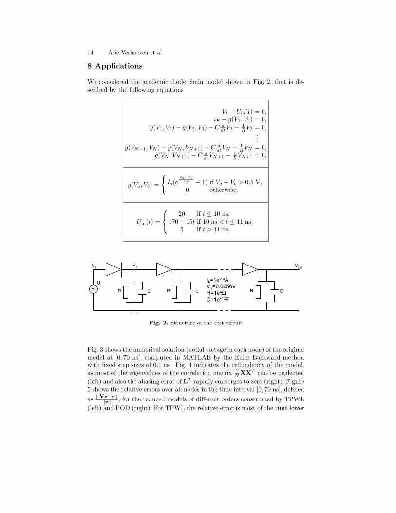
8 Applications

We considered the academic diode chain model shown in Fig. 2, that is de-scribed by the following equations

V1 − Uin(t) = 0,iE − g(V1, V2) = 0,

g(V1, V2)− g(V2, V3)− C ddtV2 − 1

RV2 = 0,...

g(VN−1, VN )− g(VN , VN+1)− C ddtVN − 1

RVN = 0,g(VN , VN+1)− C d

dtVN+1 − 1RVN+1 = 0,

g(Va, Vb) =

Is(e

Va−VbVT − 1) if Va − Vb > 0.5 V,0 otherwise,

Uin(t) =

20 if t ≤ 10 ns,170− 15t if 10 ns < t ≤ 11 ns,

5 if t > 11 ns.

R C~ R C R C

Uin

V2

V300

V1

Is=1e-14A

VT=0.0256V

R=1e4Ω

C=1e-12F

Fig. 2. Structure of the test circuit

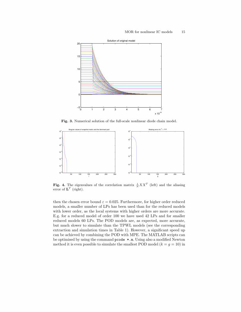
Fig. 3 shows the numerical solution (nodal voltage in each node) of the originalmodel at [0, 70 ns], computed in MATLAB by the Euler Backward methodwith fixed step sizes of 0.1 ns. Fig. 4 indicates the redundancy of the model,as most of the eigenvalues of the correlation matrix 1

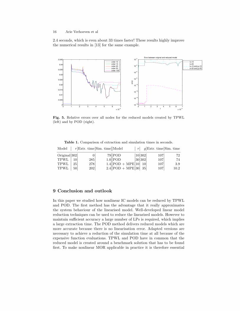
N XXT can be neglected(left) and also the aliasing error of LT rapidly converges to zero (right). Figure5 shows the relative errors over all nodes in the time interval [0, 70 ns], definedas ||Vz−x||

||x|| , for the reduced models of different orders constructed by TPWL(left) and POD (right). For TPWL the relative error is most of the time lower

MOR for nonlinear IC models 15

0 1 2 3 4 5 6 7

x 10−8

−5

0

5

10

15

20Solution of original model

Fig. 3. Numerical solution of the full-scale nonlinear diode chain model.

50 100 150 200 250 30010−8

10−6

10−4

10−2

100

102

104Singular values of snapshot matrix and the dominant part

r50 100 150 200 250 300

10−6

10−4

10−2

100

102

104Aliasing error of LT = T*P

g

Fig. 4. The eigenvalues of the correlation matrix 1N

XXT (left) and the aliasingerror of LT (right).

then the chosen error bound ε = 0.025. Furthermore, for higher order reducedmodels, a smaller number of LPs has been used than for the reduced modelswith lower order, as the local systems with higher orders are more accurate.E.g. for a reduced model of order 100 we have used 42 LPs and for smallerreduced models 60 LPs. The POD models are, as expected, more accurate,but much slower to simulate than the TPWL models (see the correspondingextraction and simulation times in Table 1). However, a significant speed upcan be achieved by combining the POD with MPE. The MATLAB scripts canbe optimised by using the command pcode *.m. Using also a modified Newtonmethod it is even possible to simulate the smallest POD model (k = g = 10) in

16 Arie Verhoeven et al

2.4 seconds, which is even about 33 times faster! These results highly improvethe numerical results in [13] for the same example.

0 1 2 3 4 5 6 7

x 10−8

0

0.005

0.01

0.015

0.02

0.025

0.03

0.035

0.04

0.045order 10order 15order 25order 50order 100

0 1 2 3 4 5 6 7

x 10−8

10−16

10−14

10−12

10−10

10−8

10−6

10−4

10−2Error between original and reduced model

t

erro

r

k=10k=30k=10 and g=10k=30 and g=35

Fig. 5. Relative errors over all nodes for the reduced models created by TPWL(left) and by POD (right).

Table 1. Comparison of extraction and simulation times in seconds.

Model r Extr. time Sim. time Model r g Extr. time Sim. time

Original 302 0 79 POD 10 302 107 72TPWL 10 285 1.0 POD 30 302 107 74TPWL 25 278 1.4 POD + MPE 10 10 107 3.9TPWL 50 202 2.4 POD + MPE 30 35 107 10.2

9 Conclusion and outlook

In this paper we studied how nonlinear IC models can be reduced by TPWLand POD. The first method has the advantage that it really approximatesthe system behaviour of the linearised model. Well-developed linear modelreduction techniques can be used to reduce the linearised models. However tomaintain sufficient accuracy a large number of LPs is required, which impliesa large extraction time. The POD method delivers reduced models which aremore accurate because there is no linearisation error. Adapted versions arenecessary to achieve a reduction of the simulation time at all because of theexpensive function evaluations. TPWL and POD have in common that thereduced model is created around a benchmark solution that has to be foundfirst. To make nonlinear MOR applicable in practice it is therefore essential

MOR for nonlinear IC models 17

that a proper benchmark solution can be calculated. This could be done by acheap integration method at a coarse time-grid or in a hierarchical way fromtypical trajectories per subcircuit. Both the MOR methods TPWL and PODseems to be promising for reducing the simulation time for nonlinear DAEsystems. They offer a good starting point for further research on MOR ofnon-linear dynamical systems.

Acknowledgment

We would like to thank Dr. B. Tasic for his help with the diode chain modeland Dr. J. Rommes for his support with the tool Hstar.

References

1. A.C. Antoulas. Approximation of Large-Scale Dynamical Systems. Society forIndustrial and Applied Mathematics, Philadelphia, 2005.

2. P. Astrid. Reduction of process simulation models: a proper orthogonal decompo-sition approach. PhD thesis, Eindhoven University of Technology, Departmentof Electrical Engineering, 2004.

3. P. Astrid and S. Weiland. On the construction of POD models from partialobservations. In Proceedings of the 44th IEEE Conf. on Decision and Control,pp 2272-2277, Spain, 2005.

4. P. Astrid, S. Weiland, K. Willcox, and A. Backx. Missing Point Estimation inmodels described by Proper Orthogonal Decomposition. In Proceedings of the43th IEEE Conf. on Decision and Control, volume 2, pp 1767-1772, Bahamas,2004.

5. P. Astrid and A. Verhoeven. Application of Least Squares MPE technique inthe reduced order modeling of electrical circuits. In Y. Yamamoto, T. Sugie, andY. Ohta, editors, Proceedings of 17th Int. Symposium on Mathematical Theoryof Networks and Systems (CDROM), pp 1980-1986, Japan, 2006.

6. P. Benner, V. Mehrmann, and D.C. Sorensen. Dimension Reduction of Large-Scale Systems. Springer-Verlag, Berlin/Heidelberg, 2006.

7. R. Everson and L. Sirovich. The Karhunen-Lueve procedure for gappy data.Journal Opt.Soc.Am., 12:1657–1664, 1995.

8. R.W. Freund. Krylov-subspace methods for reduced order modeling in circuitsimulation. Journal of Computational and Applied Mathematics, Vol. 123, pp395-421, 2000.

9. C. Homescu, L.R. Petzold, and R Serban. Error estimation for reduced-ordermodels of dynamical systems. SIAM Journal on Numerical Analysis, Vol. 43,pp 1693-1714, 2005.

10. A. Odabasioglu, M. Celik, and L.T. Pileggi. PRIMA: Passive Reduced-order In-terconnect Macromodeling Algorithm, IEEE Transactions on Computer-AidedDesign of Integrated Circuits and Systems, Vol. 17, No. 8, pp 645-654, 1998.

11. J. Phillips, and L.M. Silvera. Poor Man’s TBR: A simple model reductionscheme, IEEE transactions on computer-aided design of integrated circuits andsystems. Vol. 14, No. 1, 2005.

18 Arie Verhoeven et al

12. M. Rewienski, and J. White. A Trajectory Piecewise-Linear Approach to ModelOrder Reduction and Fast Simulation of Nonlinear Circuits and MicromachinedDevices. In Proc. of the Int. Conf. on CAD, pp 252–257, 2001.

13. A. Verhoeven. Redundancy Reduction of IC Models by Multirate Time-Integration and Model Order Reduction. PhD thesis, Eindhoven University ofTechnology, Department of Mathematics and Computer Science, Eindhoven,2008.

14. A. Verhoeven, T. Voss, P. Astrid, E.J.W. ter Maten, and T. Bechtold. Modelorder reduction for nonlinear problems in circuit simulation. Presented at theICIAM Conf., Zurich, 2007.

15. T. Voss. Model reduction for nonlinear differential algebraic equations, MSc.thesis, University of Wuppertal, 2005.

16. T. Voss, R. Pulch, E. ter Maten, and A. El Guennouni. Trajectory PiecewiseLinear Approach for Nonlinear Differential-Algebraic Equations in circuit simu-lation . In G. Ciuprina and D. Ioan, editors, Scientific Computing in ElectricalEngineering, pp 167–173, Sinaia, Romania, 2007. Springer.

17. T. Voss, A. Verhoeven, T. Bechtold, and J. ter Maten. Model order reduc-tion for nonlinear differential-algebraic equations in circuit simulation. In L.L.Bonilla, M. Moscoso, and J.M. Vega, editors, Progress in Industrial Mathematicsat ECMI 2006, pp 518–523, Madrid, Spain, 2007. Springer.

18. K. Willcox. Unsteady flow sensing and estimation via the gappy proper orthog-onal decomposition. Computers and Fluids, Vol. 35, pp 208-226, 2006.