Model of Rousselier in great deformations

Code_Aster Versiondefault

Titre : Modèle de Rousselier en grandes déformations Date : 28/10/2014 Page : 1/29Responsable : HABOUSSA David Clé : R5.03.06 Révision :

9c732cd6c72d

Model of Rousselier in great deformations

Summary

One presents here an alternative of the model of Rousselier which makes it possible to describe the plasticgrowth of cavities in a steel. The relation of behavior is elastoplastic with isotropic work hardening, allows thechanges of plastic volume and is written in great deformations. These last are based on the theory suggestedby Simo and Miehe, modified to facilitate the digital integration of the law of behavior and to replace the modelwithin the framework of generalized standard materials.This model is available in the order STAT_NON_LINE via the keyword RELATION: ‘ROUSSELIER’ under thekeyword factor BEHAVIOR and with the keyword DEFORMATION: ‘SIMO_MIEHE’.This model is established for three-dimensional modelings (3D), axisymmetric (AXIS) and in planedeformations (D_PLAN).

One presents the writing and the digital processing of this model.

Warning : The translation process used on this website is a "Machine Translation". It may be imprecise and inaccurate in whole or in part and isprovided as a convenience.Copyright 2021 EDF R&D - Licensed under the terms of the GNU FDL (http://www.gnu.org/copyleft/fdl.html)



9c732cd6c72d

Contents

Contents1 Introduction........................................................................................................................................... 3

2 Notations.............................................................................................................................................. 4

3 Theory of Simo and Miehe................................................................................................................... 5

3.1 Introduction.................................................................................................................................... 5

3.2 General information on the great deformations.............................................................................5

3.2.1 Kinematics............................................................................................................................ 5

3.2.2 Constraints............................................................................................................................ 6

3.2.3 Objectivity............................................................................................................................. 6

3.3 Formulation of Simo and Miehe.....................................................................................................7

3.3.1 Original formulation..............................................................................................................8

3.3.2 Modified formulation.............................................................................................................9

3.3.3 Consequences of the approximation....................................................................................9

4 Model of Rousselier............................................................................................................................ 11

4.1 Equations of the model................................................................................................................11

4.2 Treatment of the singular points...................................................................................................11

4.3 Expression of porosity.................................................................................................................. 12

4.4 Relation ‘ROUSSELIER‘..............................................................................................................13

4.5 Internal constraints and variables................................................................................................14

5 Digital formulation.............................................................................................................................. 14

5.1 Expression of the discretized model............................................................................................14

5.2 Resolution of the nonlinear system..............................................................................................17

5.2.1 Examination of the singular points.....................................................................................17

5.2.2 Regular solution.................................................................................................................. 18

5.3 Course of calculation................................................................................................................... 19

5.4 Resolution.................................................................................................................................... 19

5.4.1 Hight delimiters and lower if the function S is strictly positive in the beginning.................19

5.4.2 Hight delimiters and lower if the function S is negative or worthless in the beginning.......21

5.4.3 Hight delimiters and lower if the function is strictly negative in the beginning and not

solution............................................................................................................................... 22

5.5 Correction of volume a posteriori.................................................................................................23

5.6 Form of the tangent matrix of the behavior.................................................................................23

6 Bibliography........................................................................................................................................ 29

7 Description of the versions of the document......................................................................................29




9c732cd6c72d

1 Introduction

The mechanisms at the origin of the ductile rupture of steels are associated with the development ofcavities within material. Three phases are generally distinguished:

• germination: it is the initiation of the cavities, into cubes sites which correspond preferentially tothe defects of material,

• growth: it is the phase which corresponds to the development itself of the cavities, controlledprimarily by the plastic flow of the metal matrix which surrounds these cavities,

• coalescence: it is the phase which corresponds to the interaction of the cavities between them tocreate macroscopic cracks.

In what follows, we treat only the phases of growth and coalescence. Rousselier [bib1] proposed a lawof capable behavior to give an account of these two phases. Compared to this formulation of origin,Lorentz and al. [bib2] introduced several modifications relating primarily to the treatment of the greatdeformations (multiplicative decomposition), the evolution of porosity (function of the total deflection)and the expression of the law of flow at the singular point of surface threshold.

More precisely, the model is based on assumptions which introduce a microstructure made up of acavity and a plastic rigid matrix thus isochoric. In this case, porosity f , definite like the relationship

between the volume of the cavity V C and total volume V representative ground volume, is

directly connected to the macroscopic deformation by:

J=det F=1− f 0

1− f avec f=

V c

V⇔ f=1− f trD éq 1-1

where f 0 indicate initial porosity, F the tensor gradient of the transformation, J variation of

volume and D the rate of deformation.

To build the law of growth of the cavities, Rousselier took as a starting point a phenomenologicanalysis which leads it to the following ingredients:

•great deformations figure,•irreversible changes of volume,•isotropic work hardening.

These considerations lead it to write the criterion of plasticity F in the following form:

F , R = eq1 D f exp H

1−R p − y éq 1-2

where is the constraint of Kirchhoff, R isotropic work hardening function of the cumulated

plastic deformation p and 1 , D and y parameters of material. The presence in the

criterion of plasticity of the hydrostatic constraint H authorize the changes of plastic volume. One

also notices that this model does not comprise a specific variable of damage because onlymicrostructural information selected is porosity, directly related to the macroscopic deformation by theequation [éq 1-1].

As for the treatment of the great deformations, one adopts the theory of Simo and Miehe but in aslightly modified formulation. The approximations brought make it possible to make easier the digitalintegration of the law of behavior but also to replace the theory of Simo and Miehe within theframework of generalized standard materials.

Thereafter, one briefly gives some concepts of mechanics in great deformations, then one points outthe theory of Simo and Miehe as well as the made modifications. One presents finally the relations ofbehavior of the model of Rousselier and his digital integration.




9c732cd6c72d

2 Notations

One will note by:

Id matrix identity

tr A trace of the tensor With

AT transposed of the tensor With

detA determinant of With

A deviatoric part of the tensor With defined by A=A−

13

trA Id

AH hydrostatic part of the tensor With defined by AH=

trA

3:

doubly contracted product: A :B=∑i , j

Aij Bij=tr ABT

⊗ tensorial product: A⊗Bijkl=Aij B kl

Aeq equivalent value of Von Mises defined by Aeq= 32A: A

∇XA gradient : ∇ XA=∂A

∂X

, ,E , ,K moduli of the isotropic elasticity

y elastic limit

thermal dilation coefficient

T temperature

T ref temperature of reference

In addition, within the framework of a discretization in time, all the quantities evaluated at the previousmoment are subscripted by − , quantities evaluated at the moment t t are not subscripted and

the increments are indicated by . One has as follows:

Q=Q−Q−




9c732cd6c72d

3 Theory of Simo and Miehe

3.1 IntroductionWe point out here specificities of the formulation suggested by SIMO J.C and MIEHE C. [bib3] to treatthe great deformations. This formulation was already used for models of thermo-élasto behavior(visco) - plastic with isotropic work hardening and criterion of Von Mises, [R5.03.21] for a modelwithout effect of the metallurgical transformations and [R4.04.03] for a model with effect of themetallurgical transformations.The kinematics choices make it possible to treat great displacements and great deformations but alsoof great rotations in an exact way.Specificities of these models are the following ones:

•just like in small deformations, one supposes the existence of a slackened configuration, i.e.locally free of constraint, which makes it possible to break up the total deflection into athermoelastic part and a plastic part,

•the decomposition of this thermoelastic deformation into cubes parts and plastic is not additiveany more as in small deformations (or for the models great deformations written in rate ofdeformation with for example a derivative of Jaumann) but multiplicative,

•the elastic strain are measured in the current configuration (deformed) while the plasticdeformations are measured in the initial configuration,

•as in small deformations, the constraints depend only on the thermoelastic deformations,•if the criterion of plasticity depends only on the deviatoric constraint, then the plastic

deformations are done with constant volume. The variation of volume is then only due to thethermoelastic deformations,

•this model led during its digital integration to a model incrémentalement objective (cf [§3.2.3])what makes it possible to obtain the exact solution in the presence of great rotations.

Thereafter, one briefly points out some concepts of mechanics in great deformations.

3.2 General information on the great deformations

3.2.1 Kinematics

Let us consider a solid subjected to great deformations. That is to say 0 the field occupied by the

solid before deformation and t the field occupied at the moment T by the deformed solid.

Configuration actuelle déforméeConfiguration initiale

F 0 ( )t

Figure 3.2.1-a: Representation of the initial and deformed configuration

In the initial configuration 0 , the position of any particle of the solid is indicated by X(Lagrangian description). After deformation, the position at the moment t particle which occupied

the position X before deformation is given by the variable x (description eulérienne).

The total movement of the solid is defined, with u displacement, by:

x=x X ,t =Xu éq 3.2.1-1




9c732cd6c72d

To define the change of metric in the vicinity of a point, the tensor gradient of the transformation isintroduced F :

F=∂ x

∂X=Id∇X u éq 3.2.1-2

The transformations of the element of volume and the density are worth:

d=Jdo with J=det F=o

éq 3.2.1-3

where o and are respectively the density in the configurations initial and current.

Various tensors of deformations can be obtained by eliminating rotation in the local transformation. Forexample, by directly calculating the variations length and angle (variation of the scalar product), oneobtains:

E=12C−Id with C=FTF éq 3.2.1-4

A=12 Id−b− 1 with b=FFT éq 3.2.1-5

E and A are respectively the tensors of deformation of Green-Lagrange and Euler-Almansi

and C and b , tensors of right and left Cauchy-Green respectively.

In Lagrangian description, one will describe the deformation by the tensors C or E because

they are quantities defined on 0 , and of description eulérienne by the tensors b or A(definite on ).

3.2.2 Constraints

The tensor of the constraints used in the theory of Simo and Miehe is the tensor of Kirchhoff defined by:

J= éq 3.2.2-1

where is the tensor eulérien of Cauchy. The tensor thus result from a “scaling” by the

variation of volume of the tensor of Cauchy .

3.2.3 Objectivity

When a law of behavior in great deformations is written, one must check that this law is objective, i.e.invariant by any change of space reference frame of the form:

x*=c t Q t x éq 3.2.3-1

where Q is an orthogonal tensor which represents the rotation of the reference frame and c avector which represents the translation.

More concretely, if one carries out a tensile test in the direction e1 , for example, followed by a

rotation of 90° around e3 , which amounts carrying out a tensile test according to e2 , then the

danger with a nonobjective law of behavior is not to find a uniaxial tensor of the constraints in the

direction e2 (what is in particular the case with kinematics PETIT_REAC).




9c732cd6c72d

3.3 Formulation of Simo and Miehe

Thereafter, one will note F the tensor gradient which makes pass from the initial configuration

0 with the current configuration t , Fp the tensor gradient which makes pass from the

configuration 0 with the slackened configuration r , and F e configuration

r with t .

The index p refers to the plastic part, the index e with the elastic part.

Configuration initiale Configuration actuelle

Configuration relâchée

F eF p

F

r

0 ( )t

T Tref

0

Figure 3.3-a: Decomposition of the tensor gradient F in an elastic part F e and plastic Fp

By composition of the movements, one obtains the following multiplicative decomposition:

F=FeFp éq 3.3-1

The elastic strain are measured in the current configuration with the left tensor eulérien of Cauchy-

Green be and plastic deformations in the initial configuration by the tensor Gp (Lagrangian

description). These two tensors are defined by:

be=F eFeT , Gp=F pT Fp −1 from where be=FG pFT éq 3.3-2

However, one will employ alternatively another measurement of the elastic strain e who coincideswith the opposite of the linearized deformations when the elastic strain are small:

e=12Id−be éq 3.3-3

In the case of an isotropic material, one can show that the potential free energy depends only on the

left tensor of Cauchy-Green be (where in our case of the tensor e ) and in plasticity of the variable

p dependent on isotropic work hardening. Moreover, one supposes that the voluminal free energybreaks up, just like in small deformations, in a hyperelastic part which depends only on the elasticstrain and another related to the mechanism on work hardening:

e , p =el e bl p éq 3.3-4




9c732cd6c72d

So instead of using the constraint of Cauchy , one uses the constraint of Kirchhoff , theinequality of Clausius-Duhem is written (one forgets the thermal part):

:D−≥ 0 éq 3.3-5

expression in which D represent the rate of deformation eulérien.

Under the preceding assumptions, dissipation is still written:

∂∂ e be :D 12∂

∂e: FG pFT− ∂

∂ p˙p≥ 0 éq 3.3-6

The second principle of thermodynamics then requires the following expression for the relation stress-strain:

=−∂

∂ ebe éq 3.3-7

One defines finally the thermodynamic forces associated with the elastic strain and the plasticdeformation cumulated in accordance with the framework with generalized standard materials:

s=−∂

∂ e soit =s be éq 3.3-8

A=−∂Φ∂ p

éq 3.3-9

where the thermodynamic force With is the opposite of the isotropic variable of work hardening R.

It remains then for dissipation:

: −12FGpFT be− 1A p = s : −

12FG pFT A p≥ 0 éq 3.3-10

3.3.1 Original formulation

The principle of maximum dissipation applied starting from the threshold of elasticity F , function of

the constraint of Kirchhoff and of the thermodynamic force A allows to deduce the laws ofevolution from them from the plastic deformation and cumulated plastic deformation, is:

−12FGpFT be -1=

∂F∂

éq 3.3.1-1

˙p=∂F∂ A

éq 3.3.1-2

≥0 F≤0 F =0 éq 3.3.1-3




9c732cd6c72d

3.3.2 Modified formulation

The approximation introduced here on the original formulation of Simo and Miehe relates to theexpression of the law of flow, all the more reduced approximation as the elastic strain are small, since

=s be . Indeed, one henceforth expresses the threshold of elasticity like a function of the

thermodynamic forces and either of the constraints F s , A≤0 , and it is compared to thesevariables that one applies the principle of maximum dissipation, which leads to the following laws offlow:

−12FGpFT=

∂F∂ s

éq 3.3.2-1

p=∂F∂ A

éq 3.3.2-2

≥0 F≤0 F =0 éq 3.3.2-3

3.3.3 Consequences of the approximation

By replacing the constraint by the thermodynamic force s associated with the elastic strain inthe expression of the criterion of plasticity, one introduces in fact a disturbance of the border of thefield of reversibility of about size of 2∥e∥ . Compared to the initial formulation, it results from itobviously an influence on the elastic limit observed but also on the direction from flow: in particular,the derivative compared to the time of the plastic variation of volume is written then:

J p= J pbe -1 :∂ F∂ s

éq 3.3.3-1

so that if the criterion F depends only on the diverter of the tensor of the constraints s , one

does not find J p=1 : the isochoric character of the plastic deformation is not preserved perfectly any

more. We will then be brought to introduce a correction of volume a posteriori.

Insofar as the elastic strain remain small, the results got with this modified model do not deviatesignificantly from those obtained with the old formulation (cf [bib4]), while digital integration will besimplified by it. Indeed, one will see thereafter whom this model follows the same diagram ofintegration as that of the models written in small deformations.

Note:

This new formulation of the great deformations makes it possible to replace the theory ofSimo and Miehe within the framework as of generalized standard materials. From a digitalpoint of view, this results in to express the resolution of the law of behavior like a problem ofminimization compared to the internal increments of variables.

Indeed, one recalls that within the framework of generalized standard materials, the data ofthe two potentials the free energy , a and potential of dissipation D a , function of

the tensor of deformation and of a certain number of internal variables a , allows todefine the law of behavior completely (one places oneself in the case as of materialsindependent of time).

=∂

∂ , A=−

∂

∂ a∈∂ D a éq 3.3.3-2

where ∂D a is under differential of the potential of dissipation D . Warning : The translation process used on this website is a "Machine Translation". It may be imprecise and inaccurate in whole or in part and isprovided as a convenience.Copyright 2021 EDF R&D - Licensed under the terms of the GNU FDL (http://www.gnu.org/copyleft/fdl.html)



9c732cd6c72d

The laws of generalized behavior of the standard type which do not depend on time arecharacterized by a potential of dissipation positively homogeneous of degree 1, which resultsin the following property:

∀ a ∀0 D a =D a ⇒ ∂D ˙a =∂D a éq 3.3.3-3

Now if one writes the problem [éq 3.3.3-2] in form discretized in time and if one uses theproperty of under differentials [éq 3.3.3-3], one obtains the following discretized problem:

=∂

∂ , A=−

∂

∂ a∈∂ D a éq 3.3.3-4

One can show that the equation [éq 3.3.3-4] is equivalent (cf [bib5]) to solve the problem ofminimization compared to the increments of internal variables a according to:

−∂

∂a∈∂D a ⇔ a=ArgMin

a*

[a−Δa*D a*

] éq 3.3.3-5

The application of the equation [éq 3.3.3-5] to the model of Rousselier in great modifieddeformations is written:

e , p et D Dp , p énergie continue

=>discrétisation

eTr e , p− p et D e , p énergie discrétisée

éq 3.3.3-6

A=−∂

∂ a={s=−

∂

∂ e

− R=−∂

∂ p

∈∂D e , p

⇔ Min e , p

[eTr e , p− p D e , p ]

éq. 3.3.3-7

One will find in the paragraph [§4], the relation which binds the rate of plastic deformation

Dp once discretized and the increment of elastic strain e , as well as the definition of

eTr .

One sees well here whom if one takes the initial formulation of Simo and Miehe, one cannotwrite any more the problem of minimization [éq 3.3.3-7] with the constraint of Kirchhoff

because of term in be in the expression:

=−∂

∂ ebe éq 3.3.3-8




9c732cd6c72d

4 Model of Rousselier

We now describe the application of the great deformations to the model of Rousselier presented inintroduction.

4.1 Equations of the model

To describe a thermoelastoplastic model with isotropic work hardening (the equivalent in smalldeformations with the model with isotropic work hardening and criterion of Von Mises), Simo andMiehe propose an elastic potential polyconvexe. By reason of simplicity, one chooses here thepotential of Coming Saint who is written:

e , p =12[K tr e

22 e : e6K T tr e]∫

0

p

R u du éq 4.1-1

In accordance with the equations [éq 3.3-8] and [éq 3.3-9], the laws of state which derive from theelastic potential above write then:

s=− [K tr e Id2 e3K T Id ] éq 4.1-2

A=− R p éq 4.1-3

The threshold of elasticity is given by:

F s , R=seq1 Df exp sH

1− R− y éq 4.1-4

According to the equations [éq 3.3.2-1] and [éq 3.3.2-2], the laws of flow are defined by:

−12FGpFT= [ 3 s

2 seq

Df3

exp sH

σ 1Id ] éq 4.1-5

p= éq 4.1-6

≥0 F≤0 F =0 éq 4.1-7

4.2 Treatment of the singular points

In fact, the equation of flow [éq 4.1-5] translated the membership of the direction of flow to the normalcone on the surface of the field of elasticity. It is valid only at the regular points, characterized by:

seq≠0 éq 4.2-1

It thus remains to characterize the normal cone at the singular points, i.e. checking:

s=0 et 1 D f exp sH

1−R= y éq 4.2-2




9c732cd6c72d

The normal cone with convex of elasticity in such a point is the whole of the directions of flow whichcarry out the problem of maximization according to:

Δ*s ,R =sup

Dp , p[ s :Dp−R p− Dp , p ] éq 4.2-3

where * is the indicating function of the convex one F and Dp , p potential of dissipation

obtained by transform of Legendre-Fenchel of the indicating function of F :

Dp , p= Sups , R

F s , R≤0

[s :Dp−R p ]éq 4.2-4

After some calculations, one obtains:

ΔDp , p = y p1 trDp ln trDp

D f p−1 Iℝ trD

p Iℝ p−

23

Deqp éq 4.2-5

with

Iℝ x ={0 si x≥0

+ ∞ sinonéq 4.2-6

For s=0 , Δ* is worth:

Δ* s , R = SupDp

, ptrDp≥0

p−23

Deqp≥0

[s H trDp−1 trDp ln trDp

D f p−1

G trDp

−R p− y p ] éq 4.2-7

By noticing that for trDp≥0 , the function G trDp is concave, the suprémum compared to the

trace of the rate of plastic deformation Dp is obtained for:

G' trDp=0 d'où trDp=Df p exp s H

1 éq 4.2-8

Note:

One finds well then for the indicating function of the threshold of elasticity F .

D* s ,R = Supp

p≥23

D eqp≥0

[F p ]={ 0 si F≤0+∞ sinon éq 4.2-9

In a singular point, the normal cone, together of the acceptable directions of flow, is thus characterizedby:

trDp=D f p exp sH

1 éq 4.2-10

p≥ 23

Deqp≥0 éq 4.2-11

4.3 Expression of porosity




9c732cd6c72d

One saw in introduction that the microscopic inspiration of the model of Rousselier is based on amicrostructure made up of a cavity and a plastic rigid matrix, therefore isochoric. In this case, porosityis directly connected to the macroscopic deformation by the relation eq. 1-1.

In this expression, the change of elastic volume of origin is neglected. Without special precaution, thisapproximation can prove penalizing in the presence of elastic compression, even reasonable, becauseit leads to a possibly negative porosity.

One thus prefers the following equivalent expression to him, together with an explicit decrease byinitial porosity:

f =max f 0,1−1− f 0

J éq 4.3-1

Rousselier proposes as for him to express porosity while basing himself on the rate of plasticdeformation Dp . The relation is written in incremental form:

f =1− f trDp éq 4.3-2

That means that variable porosity employed to parameterize the criterion of plasticity F dependsonly on the plastic deformation. In fact, the rate of plastic deformation is a quantity evaluated in theslackened configuration. Its transport in the current configuration (like D ) still express yourself:

FeDpFeT

=−12FG pFT éq 4.3-3

In this case, the law of evolution of porosity is expressed:

f =1− f tr −12FG pFT éq 4.3-4

To avoid that the integration of porosity does not interfere with that of plasticity (since the two variablesare coupled), it is necessary to separate integration from the law of behavior in two times: integrationof plasticity with porosity fixed at its value at the beginning of the step of time, then integration ofporosity by means of the equation 4.3-4 where the plastic evolution is that calculated with thepreceding phase.

Notice important:

There are thus two possible versions of the model (PORO_TYPE = 1 or 2, cf U4.43.01), according towhether one respectively chooses the total deflection or the plastic deformation in the evolution ofporosity. It was noticed that for an initial porosity f0 low, the behavior at the beginning of evolutionstrongly changes according to this parameter. Indeed, the choice seems to have an impactdetermining on the answer at the level of the structure, since it privileges or not the junctions of thezone where the deformations are located. Thus, this strong sensitivity must lead the user to a greatestcaution in the use of this model. Research is in hand to understand this sensitivity and to discriminatethe two alternatives for the evolution of porosity.

4.4 Relation ‘ROUSSELIER‘

This relation of behavior is available via the argument ‘ROUSSELIER‘keyword BEHAVIOR under theoperator STAT_NON_LINE, with the argument ‘SIMO_MIEHE‘keyword factor DEFORMATION.




9c732cd6c72d

The whole of the parameters of the model is provided under the keywords factors ‘ROUSSELIER‘or‘ROUSSELIER_FO‘and ‘TRACTION‘(to define the traction diagram) order DEFI_MATERIAU([U4.43.01]).

Notice :

The user must make sure well that the “experimental” traction diagram used, either directly,or to deduce the slope from it from work hardening is well given in the plan forced rational

=F /S - deformation logarithmic curve ln 1 l / l0 where l 0 is the initial length of

the useful part of the test-tube, l variation length after deformation, F the force applied

and S current surface.

4.5 Internal constraints and variables

The constraints are the constraints of Cauchy, thus calculated on the current configuration (sixcomponents in 3D, four in 2D).

Internal variables produced in Code_Aster are:

•V1, cumulated plastic deformation p ,•V2, porosity f ,•V3, the indicator of plasticity (0 if the last calculated increment is elastic, 1 if regular plastic

solution, 2 if singular plastic solution),•V4 with V9, the tensor of elastic strain e .

Notice :

If the user wants to possibly recover deformations in postprocessing of his calculation, it isnecessary to trace the deformations of Green-Lagrange E , which represents ameasurement of the deformations in great deformations (option EPSG_ELGA or EPSG_ELNOCALC_CHAMP). Linearized deformations classics measure deformations under theassumption of the small deformations and do not have a direction in great deformations.

5 Digital formulation

For the variational formulation, it is same as that given in the note [R5.03.21] and which refers to thelaw of behavior with isotropic work hardening and criterion of Von Mises in great deformations. Werecall only that it is about a eulérienne formulation, with reactualization of the geometry to eachincrement and each iteration, and that one takes account of the rigidity of behavior and geometricalrigidity.We now present the digital integration of the law of behavior and give the form of the tangent matrix(options FULL_MECA and RIGI_MECA_TANG).

5.1 Expression of the discretized model

Knowing the constraint − , cumulated plastic deformation p− , elastic strain e− , displacements

u− and u , one seeks to determine , p ,e .

Displacements being known, gradients of the transformation of 0 with − , noted F− , and of

− with , noted F , are known.

To integrate this model of behavior, one employs a diagram of implicit Euler, porosity being an explicitfunction of the deformation via equation 4.3-1, therefore known during the integration of the behavior.

Once discretized, the following system then is obtained:




9c732cd6c72d

F= FF− éq 5.1-1

J=detF éq 5.1-2

J = éq 5.1-3

=s b e éq 5.1-4

be=Id−2e éq 5.1-5

•Equations of state:

s=− [2 eK tr e Id3K T Id ] éq. 5.1-6

A =−R p éq 5.1-7




9c732cd6c72d

Thereafter, one expresses the laws of flow and the criterion of plasticity directly according to thetensor of the elastic strain e .

•Laws of flow

Dp≃−12FGpFT=− 1

2 t [FGp FTbe

−FF−G p-F−Tbe−

FT] =−

12 t

[Id−2e− F {Id−2e− } FT ]

=e−12[Id− F {Id−2e− } FT ]

eTr

/ t= e−eTr / t

éq 5.1-8

By taking the parts traces and deviatoric of the equation [éq 4.1-5], one obtains:

tr e−tr eTr= p D f exp−3 K T1

exp−K tr e1

éq 5.1-9

e={eTr −3

2 p e

eeq

si solution régulière

0 et Δp≥23 e−eTr eq si solution singulière

éq 5.1-10

•Conditions of coherence

F={2 eeq1 D f exp −3 K T1

exp−K tr e1

−R− y si solution régulière

1 D f exp−3 K T 1

exp −K tr e 1

−R− y si solution singulière

avec F≤0 p≥0 F p=0

éq 5.1-11




9c732cd6c72d

5.2 Resolution of the nonlinear system

The integration of the law of behavior is thus summarized to solve the system [éq 5.1-9], [éq 5.1-10]and [éq 5.1-11]. We will see that this resolution is brought back to that of only one scalar equation, ofwhich the unknown factor x is the increment of the trace of the elastic strain:

x=tr e−tr eTr éq 5.2-1

Thanks to this choice, that the solution is elastic or plastic, attack in a singular point or not, theequation [éq 5.1-9] bearing on the trail of the elastic increment is always valid and makes it possible toexpress the increment of cumulated plastic deformation:

tr e−tr eTr= p D f exp−K tr eTr

1exp−3 K T

1

G

exp −K tr e−tr eTr

1

⇒ p x =1G

x expK x1

éq 5.2-2

This equation shows us that one can seek x≥0 to guarantee a positive cumulated plasticdeformation and that the elastic solution is obtained for x=0 . One also notices that the incrementof cumulated plastic deformation is a function continuous and strictly increasing of x . With the

help of these remarks, if one notes by S the term [éq 5.2-3] in the criterion of plasticity, it acts then,there too, of a continuous and strictly increasing function of x :

F=2 eeq−S x avec S x =−1 G exp−Kx 1R p x y éq 5.2-3

This stage, the approach of resolution breaks up into two times.

5.2.1 Examination of the singular points

Such a singular point is characterized by [éq 5.1-10] (low) and [éq 5.1-11] (low), therefore in particularby S x =0 . Because of the properties of S , this equation admits with more the one positive

solution, say x S who exists if and only if S 0 ≤0 . The knowledge of x S allows to deduce the

tensor from it from elastic strain e , cumulated plastic deformation p as well as thethermodynamic forces s and R .

Finally, this singular point will be solution if the inequality in [éq 5.1-11] (low) is checked, i.e. if:

Δps≥

23 es−eTr

eq éq 5.2.1-1




9c732cd6c72d

5.2.2 Regular solution

The equation of flow [éq 5.1-10] (high) which determines the deviatoric part of the tensor of elasticstrain makes it possible to deduce a scalar equation from it function from the increment of cumulatedplastic deformation:

e−eTr=−

32

Δp eeeq

⇒ {eeq=eeqTr−

32 p

e=eeq

eeqTr e

Tréq 5.2.2-1

One notes that because of positivity of eeq , the value sells by auction p is limited:

p≤ 23

eeqTr

éq 5.2.2-2

The condition of coherence determines now x :

F=2 eeqTr−S x −3 p ≤0 éq 5.2.2-3

Being given this expression, the increase of the value sells by auction p is reduced to the only

condition S x ≥0 or, in an equivalent way, with x≥x S .

The elastic solution is obtained for x = 0. It is the solution of the problem if and only if:

F 0 =2 eeqTr−S 0 0 éq 5.2.2-4

In the contrary case, one must then solve:

F x =2 eeqTr−S x −

3G

x expKx 1

=0 avec {xx s si x s existex0 sinon

éq 5.2.2-5

This function is continuous and strictly decreasing and tends towards −∞ with x . She thusadmits with more the one solution. The demonstration of the existence of this solution is immediate.Indeed, it is enough to prove that F is positive on the lower limit of the interval of research.

When x S do not exist, F 0 0 since the solution is not elastic.

When x S exist, the function is worth:

F x s=2 eeq

Tr−3 ps

0⇔ p s

23

eeqTr

éq 5.2.2-6

This condition is checked since the singular solution was rejected.




9c732cd6c72d

5.3 Course of calculation

The approach to solve the whole of the equations of the model is the following one:

1) One searches if the solution is elastic•calculation of F 0 •if F 0 0 , the solution of the problem is the elastic solution x Sol=0•if not one passes in 2)

2) If S 0 0 , the solution is plastic and regular•one passes in 4)

3) If S 0 0 , one seeks if the solution is singular

•one solves S x s =0

•if x s check the inequality Δps≥

23 es−eTr

eq , then the solution is singular x Sol=x s

•if not, x s is a lower limit to solve F x =0 , one passes in 4)4) The solution is plastic and regular

•one solves F x =0

5.4 Resolution

To solve the two equations S x =0 and F x =0 , one employs a method of Newton withcontrolled terminals coupled to dichothomy when Newton gives a solution apart from the interval ofthe two terminals. One now presents the determination of the terminals for each preceding case (items2) 3) and 4) preceding paragraph).

5.4.1 Hight delimiters and lower if the function S is strictly positive in the beginning

One solves:

{F x =0F 00

⇔{2 eeqTr−S x f 1

=3G

x expKx 1

3 p

f 1 0 0

éq 5.4.1-1

where the function Δp x is continuous, strictly increasing and worthless at the origin and the

function f 1 x is continuous, strictly decreasing and strictly positive at the origin (see [Figure 5.4.1-a]).One poses:

f 1=2 eeqTr−R x − y

f 2

1 Gexp − Kx1

alors f 2 x f 1 x ∀ x≥0 éq 5.4.1-2




9c732cd6c72d

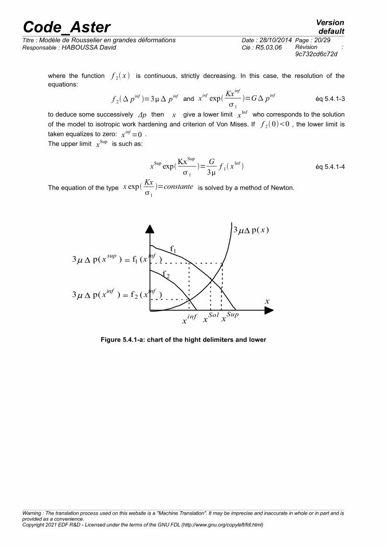
where the function f 2 x is continuous, strictly decreasing. In this case, the resolution of theequations:

f 2 pinf =3 pinf and xinf expKx inf

1

=G pinféq 5.4.1-3

to deduce some successively Δp then x give a lower limit x Inf who corresponds to the solution

of the model to isotropic work hardening and criterion of Von Mises. If f 200 , the lower limit is

taken equalizes to zero: xinf=0 .

The upper limit xSup is such as:

xSup expKxSup

1

=G3

f 1 xInf éq 5.4.1-4

The equation of the type x exp Kx1

=constante is solved by a method of Newton.

Solxinf

x

x

Supx

)p(3 x

1f

2f

)(f)p(3 2infinf xx

)(f)p(3 1infsup xx

Figure 5.4.1-a: chart of the hight delimiters and lower




9c732cd6c72d

5.4.2 Hight delimiters and lower if the function S is negative or worthless in thebeginning

The system to be solved is the following:

{S x =0S 0 0

⇔ {R p−xG

exp Kx1

y=1 Gexp−Kx 1

R p− y 1G

éq 5.4.2-1

The part of left is a continuous function, strictly increasing of x and strictly positive in thebeginning, the part of right-hand side is a continuous function, strictly decreasing of x and strictlypositive at the origin. Using the properties of these two functions, a chart (cf [Figure 5.4.2-a]) of thesefunctions shows that the upper limit xSup is such as:

1 G exp −KxSup

1

=R p− y ⇔ x Sup=1

Klog 1 G

R p− y éq 5.4.2-2

The lower limit x Inf is such as:

1 G exp −Kx Inf

1

=R p−x Sup

Gexp

Kx Sup

1

y

⇔ x Inf=⟨ 1

Klog

1G

R p−x Sup

Gexp

KxSup

1

y ⟩

éq 5.4.2-3

xInf

xSup

xSol

x

yx )R(

yp )R(

G1

)exp(G1

1

Kx





9c732cd6c72d

5.4.3 Hight delimiters and lower if the function S is strictly negative in thebeginning and x s not solution

The following system is solved:

{F x =0S 0 0S x s =0

⇔ {2 eeq

Tr−S x f 1

=3G

x expKx1

3 p

f 100

2 eeqTr=

3G

x s expKx s

1

éq 5.4.3-1

The solution x Sol is such as S x Sol 0 .

For the lower limit, one takes x Inf=x s . Being given properties of the functions f 1 (strictly

decreasing) and 3 p x (strictly increasing), the upper limit x Sup is such as (cf [Figure 5.4.3-a]):

x Sup expKxSup

1

=2G3

eeqTr

éq 5.4.3-2

This equation is solved by a method of Newton.

xSupxSolx

)exp(3

1 Kx

xG

)0(Se2 Treq

0)( xS

0)( xS

0)( xS

Treqe2

sInf xx





9c732cd6c72d

5.5 Correction of volume a posteriori

In the case of the model of Rousselier, the change of volume plays a crucial role, so that the mistakemade by the approximation s= in the equations of flow can lead to an evolution can precise ofporosity, cf [Bib2]. While following the proposal for this reference, one will correct a posteriori (i.e afterhaving calculated all the quantities) the trace of the elastic strain.

Indeed, in the absence of approximation, the hydrostatic part of the equation of flow leads to:

ddt

ln J p = p D f exp tr 31 (éq. 5.5-1)

After discretization in time, one then obtains a proposal corrected for the changes of plastic and elasticvolume:

J corrp=J p - exp tr e−tr eTr ; J corr

e=

JJ corr

p (éq. 5.5-2)

One then will seek a new trace of elastic strain such as the elastic change of volume correspondsto the value corrected above:

ecorr=et Id où t tel que : det Id−2ecorr =J corre 2 (éq. 5.5-3)

That led to a polynomial of degree 3 in t , of which one will choose the solution nearest to e .

5.6 Form of the tangent matrix of the behavior

One gives the form of the tangent matrix here (option FULL_MECA during iterations of Newton, optionRIGI_MECA_TANG for the first iteration). For the option FULL_MECA, this one is obtained by linearizing the system of equations which governsthe law of behavior. We give hereafter the broad outlines of this linearization.For the option RIGI_MECA_TANG, it is the same expressions as those given for FULL_MECA but with

p=0 . In particular, one will have F=Id .

The law of behavior can be put in the following general form:

= , F éq 5.6-1

= e éq 5.6-2

e=e eTr , f éq 5.6-3

eTr=eTr F éq 5.6-4

The linearization of this system gives:

= ∂∂ :∂∂e

: ∂e∂eTr :∂eTr

∂ F∂e∂ f

∂ f∂ J⊗∂ J∂ F ∂

∂ F :F=H : F éq 5.6-5




9c732cd6c72d

where H is the tangent matrix. Thereafter, one separately determines the five terms of thepreceding equation.In the linearization of the system, one will often use the tensor C defined below and two followingequations:

δaij=12δ ik δ jlδ jk δ il δakl éq 5.6-6

δ a pp=δ kl δ akl éq 5.5-7

C ijkl=12δ ik δ jlδ jk δ il éq 5.6-8

•Calculation of ∂

∂ and of

∂

∂ F

Linearization of the relation which binds the constraint of Cauchy and the constraint of

Kirchhoff give:

J = ⇔ =1J −J ⊗ ∂ J

∂ F : F éq 5.6-9

By using the relation [éq 5.6-6], one obtains for ∂

∂ :

∂

∂=C éq 5.6-10

and for ∂

∂ F :

∂

∂ F=−

J⊗∂ J∂ F

éq 5.6-11

with∂ J∂ F 11

=ΔF 22 ΔF 33−ΔF 23 ΔF 32

∂ J∂ F 22

=ΔF 11 ΔF 33−ΔF 13 ΔF 31

∂ J∂ F 33

=ΔF 11 ΔF 22−ΔF 12 ΔF 21

∂ J∂ F 12

=ΔF 31 ΔF 23−ΔF 33 ΔF 21 ∂ J∂F 21

=ΔF 13 ΔF 32−ΔF 33 ΔF 12

∂ J∂ F 13

=ΔF 21 ΔF 32−ΔF 22 ΔF 31 ∂ J∂F 31

=ΔF 12 ΔF 23−ΔF 22 ΔF 13

∂ J∂ F 23

=ΔF 31 ΔF 12−ΔF 11 ΔF 32 ∂ J∂F 32

=ΔF 13 ΔF 21−ΔF 11 ΔF 23

éq 5.6-12




9c732cd6c72d

•Calculation of ∂∂e

The relation which binds the constraint of Kirchhoff and the tensor of elastic strain e isgiven by:

=s be=−2 e− Tr e Id4 e e2 tr e e - 3K T Id6K T e

éq 5.6-13

One obtains after linearization:

=2 tr e−3K T e 2e−Id Tr e 4 e ee e éq 5.6-14

from where

∂ ij

∂ekl

=2 tr e−3K T C ijkl 2eij− ij kl2 ik elj il ekjeilkje ik jl éq 5.6-15

•Calculation of ∂eTr

∂ F

The relation between the tensor of elastic strain eTr and the increment of the gradient of the

transformation F is written:

eTr=12Id− Fbe− FT éq 5.6-16

Its linearization gives:

∂ eijTr

∂ F kl

=−12 ik F jp bpl

e- F ip bpl

e- jk éq 5.6-17

•Calculation of ∂e∂eTr

Elastic case

In the elastic case, the calculation of ∂e∂ eTr

is immediate since e= eTr from where

∂e∂eTr

=C éq 5.6-18




9c732cd6c72d

Plastic case – regular Solution

To determine ∂e∂eTr

, one operates in two stages. By the law of flow discretized, one calculates in

first e according to eTr and p . Then the condition of coherence makes it possible to

deduce some p according to eTr . These two stages are thereafter detailed.The deviatoric part of the law of flow discretized is written:

e−eTr=−

32 p e

eeq

éq 5.6-19

One obtains after linearization:

132 peeq

1/α

e= eTr−32e

eeq

p94 p

e

eeq3 e : e

éq 5.6-20

To determine e : δ e , one contracts the equation [éq 5.6-20] with e what gives:

e : e=e : eTr−eeq p éq 5.6-21

from where

e=[ 9 p

4 eeq3 e⊗eC]A 1

: eTr−

32e

eeqA2

δΔpéq 5.6-22

For the part law of flow traces discretized, one a:

Tr e−TreTr=D f pexp 3 K T1

exp − K1

Tr e éq 5.6-23

what gives, while posing k 1=1D f K p 1

exp 3 K T1

exp− K 1

Tr e :

tr e=

1k 11

tr eTr

D f exp −K 1

tr e exp 3 K T 1

k 12

p

pexp −K1

tr eexp 3 K T1

k 11

D f

éq 5.6-24




9c732cd6c72d

In the plastic case, the condition of coherence is worth:

2 eeqD f 1 exp − 3 K T1

exp− K 1

Tr e−R− y=0 éq 5.6-25

from where

3eeq

e : e D 1 exp−3 K T1

exp−K tr e1

f

−D f K exp−3 K T 1

exp −K tr e1

tr e−h p=0

éq 5.6-26

By injecting the relation [éq 5.6-21] in the equation above, one obtains then, while posing

k 2=3h2 D f K exp −3 K T1

exp− K 1

Tr e :

p=

3eeq

1k 23

e : eTr−

1 D f K exp−3 K T1

exp − K1

Tr ek 24

tr eTr

exp−3 K T 1

exp −K1

Tr e 1−1 D f K

k 22

D f

éq 5.6-27

While replacing p by his value obtained above in the equations [éq 5.6-22] and [éq 5.6-24],one obtains:

e=[A1A2132 Id⊗ 33

eeq

e]ddvetr

: eTr[ 13 1 Id4 A2 132Id ]

dtretr

tr eTr

[ 13 1 Id2A2132Id ]D

dedf

f

éq 5.6-28

from where

∂ e

∂eTr=ddvetrdtretr−1

3ddvetr : Id ⊗Id éq 5.6-29

Plastic case – singular Solution

The approach is identical to that used previously.One obtains for the law of flow discretized:

e=0 ⇔ e=0 éq 5.6-30




9c732cd6c72d

for the deviatoric part and the part traces, the relation is identical to that found for the regularsolution.

tr e=1 tr eTr2 p1 D f éq 5.6-31

where 1 , 2 and 1 the same definitions as in the preceding paragraph have.

The condition of coherence then makes it possible to find p according to ∂eTr .

D f 1 exp 3K T1

exp− K1

Tr e −R− y=0 éq 5.6-32

maybe after linearization:

p=4 treTr2 D f éq 5.6-33

that is to say finally:

e= 13[142 ] Id tr eTr

dtretr

13[122 ] Id D f

dedf

éq 5.6-34

from where

∂ e∂eTr

=dtretr⊗Id éq 5.6-35

•Calculation of ∂ f∂ J

Taking into account relation 4.3-1, the derivative is written simply:

{∂ f∂ J=D

1− f 0

J 2si f f 0

∂ f∂ J=0 si f = f 0

éq 5.6-36

Note:

The tangent matrix is not deteriorated by the correction of volume because this one is carried out aposteriori, i.e. after the calculation of the constraints.




9c732cd6c72d

6 Bibliography

1) ROUSSELIER G.: “Finite constitutive deformation relations including ductile fractureramming, In three dimensional constitutive relations and ductile fracture”, ED.Nemat-Nasser, North Holland publishing company, pp. 331-355.

2) LORENTZ E., BESSON J., CANO V., “Numerical simulation of ductile fracture: efficientyear and robust constitutive implementation of the Rousselier law”, comp. Meth.Appl. Mech. Engrg. 197, pp. 1965-1982, 2008.

3) SIMO J.C., MIEHE C., “Associative coupled thermoplasticity At finite strains:Formulation, numerical analysis and implementation”, comp. Meth. Appl. Mech.Eng., 98, pp. 41-104, North Holland, 1992.SIDOROFF F., “Course on the greatdeformations”, Report Greco n51, 1982.

4) LORENTZ E., CANO V.: “With minimization principle for finite strain plasticity:incremental objectivity and immediate implementation”, Com. Num. Meth. Eng.18, pp. 851-859, 2002.

5) MIALON P.: “Elements of analysis and digital resolution of the relations of the élasto -plasticity “, EDF, bulletin of DER, data-processing series C mathematical, 3, pp.57-89, 1986

7 Description of the versions of the document

Version Aster

Author (S) orcontributor (S),organization

Description of the modifications

6.0 V.Cano, E.LorentzEDF/R & D /AMA

Initial text

9.4 E.Lorentz EDF/R & D/SINETICS

Modification of L” expression of porosity, function of change ofvolume J (what makes the model entirely implicit) and introductionof a correction on the elastic change of volume a posteriori.

12.1 J.M.Proix EDF/R & D/AMA

Card 19650: modification about the internal variables


Documents

Model of Rousselier in great deformations