Embed Size (px)
Citation preview

8/12/2019 Model of Housing Supply
http://slidepdf.com/reader/full/model-of-housing-supply 1/53
A Dynamic Model of Housing Supply∗
Alvin Murphy†
Olin Business School
Washington University in St. Louis
Spring 2010
Abstract
Housing markets often exhibit a high degree of volatility in prices and quantities, with
significant economic consequences for both homeowners and the construction sector. While
aggregate housing market patterns have been well-documented, our understanding of the
microfoundations of housing markets, particularly the timing of housing supply responses to
demand shocks, is limited. In order to shed light on the primitives underlying these patterns,
I develop and estimate the first dynamic microeconometric model of housing supply. In
the model, parcel owners choose the optimal time and nature of construction, taking into
account their expectations about future prices and costs. While retaining computational
tractability, the model includes a large state space, allows profits to vary at a very fine level of
geography, and incorporates a much broader definition of costs than previous work. Estimates
of the model, using a rich data set on individual land parcel owners in the San Francisco
Bay Area, indicate that changes in the value of the right-to-build are the primary cause
of house price appreciation and that the demographic characteristics of existing residents
are determinants of the cost environment. I find that fluctuations in broadly defined cost
variables, which include regulation costs, are key to understanding when and where building
occurs. A counterfactual simulation suggests that without pro-cyclical costs and forward-
looking behavior, construction volatility would be substantially greater.
∗This paper was part of my Ph.D. dissertation at Duke University. I am very grateful to my advisor, PatBayer, and committee members, Peter Arcidiacono, Tom Nechyba, Chris Timmins, and Jake Vigdor for advice,
encouragement, and comments. I also thank Paul Ellickson, Rob McMillan, Jan Rouwendal, Andrew Sweeting,participants of Duke’s Applied Microeconomics lunch groups, the North American Regional Science Council An-nual Meeting, Econometric Society Winter Meetings, and seminar participants at Boston College, Brown, CarnegieMellon, Claremont McKenna, Federal Reserve Board of Governors, New York University, Kellogg School of Man-agement, Olin Business School, U.B.C., U.C.L.A., University of Pennsylvania, University of Missouri, SUNY atAlbany, and Wharton for their helpful comments. I am grateful to Jon James for G.I.S. assistance and to JoeGyourko for sharing data from Gyourko and Saiz (2006). All errors are my own.
†Olin Business School, Washington University, Box 1133, St. Louis, M0 63130. Phone: (314) 935-6306. email:[email protected].
1

8/12/2019 Model of Housing Supply
http://slidepdf.com/reader/full/model-of-housing-supply 2/53
1 Introduction
Housing markets often exhibit a high degree of volatility in prices and quantities, with significant
economic consequences for both homeowners and the construction sector. Comparing the first
six months of 2007 with the first six months of 2006, for example, housing price appreciation
rates fell by almost two-thirds and housing starts fell by over a quarter.1 As an asset, housing
constitutes two thirds of the average household’s portfolio,2 meaning that the typical household
faces a large uninsurable risk from price volatility, with correspondingly large welfare effects; and
on the supply side, construction volatility has substantial direct impacts on employment levels
and the demand for raw materials.3
Cyclical patterns are a consistent feature of housing markets, with alternating periods of price increases and downturns often being evident.4 The cyclicality of housing markets naturally
arises through the interaction of demand and supply forces. Suppose a demand shock, such as
a shock to wages, pushes up prices. Because supply is then slow to respond, prices continue
rising and overshoot; and when supply eventually responds fully, prices mean-revert. These
patterns have been carefully documented using aggregate data. As Glaeser and Gyourko (2007)
convincingly show, future house prices tend to be strongly predictable, being serially correlated
in the short run and displaying mean-reversion in the medium run.
In this dynamic process, the determinants of the timing of the supply response are not well-
understood, even though the timing of supply responses is central to the length and severity
of housing cycles. To complement research that has used aggregate data to document housing
market cycles, this paper sets out a micro-oriented approach designed to shed light on the way
individual behavior helps drive the dynamics of the housing market. Accordingly, I develop and
estimate the first dynamic microeconometric model of housing supply with a rich new housing
data set.
In the model, the owners of parcels of land maximize the discounted sum of expected per-
1Sources: U.S. Census Bureau, http://www.census.gov/const/www/quarterly starts completions.pdf, andOFHEO, http://www.ofheo.gov/media/hpi/2q07hpi.pdf
2Tracy, Schneider, and Chan (1999) report the portfolio share figure.3According to the BLS, http://www.bls.gov/news.release/empsit.nr0.htm, employment in the construction
sector fell by almost 125,000 in the past year.4The Bay Area, which provides the focus for this study, experienced high price growth in the late 1970s, the
late-1980s, and since the mid-1990s, with downturns in the early-1980s and early-1990s.
2

8/12/2019 Model of Housing Supply
http://slidepdf.com/reader/full/model-of-housing-supply 3/53
period profits by choosing the optimal time and nature of construction. Each period, parcel
owners make two decisions: they decide whether or not to build a house upon their parcel and,
conditional on building, they choose the size (or type) of the house. In addition to currentprofits, parcel owners take into account their expectations about future returns to development,
balancing expected future prices against expected future costs. The outcomes generated by the
parcel owners’ profit maximizing behavior, in addition to observable sales prices, allow me to
identify the parameters of the per-period profit function, allowing profits to vary at a fine level
of geography.5
While existing housing supply models typically use aggregate time-series data, a key contri-
bution of this paper is the use of micro data on individual land parcel owners to look at the
microfoundations of housing supply. I have assembled a new data set by merging observed real
estate transactions data with geo-coded parcel data for the Bay Area over the period 1988-2004. 6
In the combined data set, I observe which parcels of land get developed, and if a parcel is built
upon, I also observe when the house was built and characteristics of the house. The analysis
focuses on the development of individual parcels, where this type of infill construction covers
approximately fifty percent of all single family residential construction over the sample period.7
Certain features of housing markets present potential obstacles to estimation. Given that
housing prices have a predictable component, it is important to capture all the relevant infor-
mation that parcel owners use to predict future prices.8 In the context of a dynamic discrete
choice model, this necessitates a very large state space, making traditional full-solution estima-
tion infeasible. I overcome this problem by using a two-step (conditional choice probability)
estimator based on Hotz and Miller (1993) and Arcidiacono and Miller (2008). Another feature
of housing markets that presents a potential estimation difficulty is the fine level of geography
at which house prices and costs vary, making the number of parameters to be estimated pro-
hibitively large in the context of a dynamic discrete choice estimator. The solution I use involves
5Many of the profit function parameters are Census tract specific.6The transactions data are drawn from a national real estate data company and provide information on every
housing unit sold in the core counties of the Bay Area. The parcel data are drawn from the California StatewideInfill Study conducted in 2004-2005 by the Institute of Urban and Regional Development at the University of California at Berkeley.
7I exclude large housing developments or new subdivisions.8See Case and Shiller (1989).
3

8/12/2019 Model of Housing Supply
http://slidepdf.com/reader/full/model-of-housing-supply 4/53
taking advantage of the separability of the log likelihood functions governing observed prices,
housing services, and construction, and estimating the model in three stages, where many of
the parameters are estimated in stages prior to the dynamic discrete choice estimation. Onefinal estimation issue is that the fixed costs of construction, which are parameters estimated
within the dynamic discrete choice estimation routine, are time-varying; this is analogous to
the time-varying brand parameters in industrial organization papers such as Gowrisankaran and
Rysman (2006). A contribution of this paper is to incorporate expectations about future fixed
cost parameters within a two-step estimation routine.
The model returns four distinct results relating to prices, variable costs, cross-sectional vari-
ation in fixed costs and the time pattern of fixed costs. The price estimates indicate that changes
in the value of the right-to-build play the primary role in the increase in house prices. Between
1988 and 2004, the typical house value doubled in real terms, whereas the marginal price of an
additional square foot of living space remained constant. These results are consistent with the
theoretical implications of Glaeser, Gyourko, and Saks (2005), who suggest that regulation is
responsible for increasing house prices.
Estimates of the overall levels of variable physical construction costs are similar to cost
indexes derived from input prices. However, I find that variable costs vary pro-cyclically over the
time period, suggesting that costs are more responsive to overall metropolitan area construction
levels than previous studies suggested.
Prices and variable construction costs do not fully explain observed construction patterns.
I therefore estimate parameters of the broader cost environment, which vary considerably by
geographic area and through time. These cost environment parameters (or fixed costs) capture
any additional costs, such as set-up costs and the regulatory environment. The cross-sectional
variation in the cost environment suggests that existing home owners influence the regulatory
environment: I find that it is more difficult to develop land in communities characterized by
higher rates of home ownership. However, neighborhood racial composition and education levels
do not have any effect on costs.
While the ability of agents to forecast housing prices has been well-documented since Case
and Shiller (1989), less has been written about the effect of time-varying costs. Using estimates
of the model, I can distinguish between the effects of expected future cost changes and expected
4
8/12/2019 Model of Housing Supply
http://slidepdf.com/reader/full/model-of-housing-supply 5/53
future price changes and shed light on one of the empirical puzzles of the housing market - what
determines construction volatility levels? A feature of the data is how quickly construction levels
increase once prices begin to rise. Given that landowners can only develop their land once, andthat prices are somewhat predictable in the short- to medium-run, a simple model would suggest
that land owners should wait for higher prices before developing their land. In practice in the
Bay Area, once house prices begin to pick up in the mid-1990s, construction levels also pick up.
Therefore, many parcel owners developed parcels in the mid-to-late-1990s at prices much lower
than they would have expected to receive if they had waited.
I examine the role of expectations about future costs in a counterfactual experiment. As I
estimate a structural model, I can simulate what construction patterns would have looked like
if land owners were not forward-looking in terms of the overall cost environment. The results
provide an important insight into the decision of parcels owners regarding when to develop their
land. Without forward looking behavior, land owners wait for much higher prices before building.
The implication is that without pro-cyclical costs and forward-looking behavior, construction
volatility would be substantially greater. That is, pro-cyclical costs provide an incentive for
some land owners to build before price peaks, as waiting for higher prices implies also waiting
for higher costs.
The remainder of the paper proceeds as follows. Section 2 examines the existing literature.
Section 3 introduces the parcel, building, and sales data I use to estimate the model. Section
4 specifies the model of housing supply (when and how parcel owners choose to develop their
land), and Section 5 explains the estimation procedure. Section 6 presents the results of the
model. Section 7 examines the implications of dynamic behavior, and Section 8 concludes.
2 Related Housing Supply Literature
While it remains true that the majority of the housing literature is concerned with demand-side issues, increasing attention is now being diverted in an effort to better understand housing
supply. In particular, the literature has been growing since the review article of DiPasquale
(1999).9
9The discussion of the pre-1999 housing literature draws on DiPasquale’s review.
5

8/12/2019 Model of Housing Supply
http://slidepdf.com/reader/full/model-of-housing-supply 6/53
In addition to early literature, such as Muth (1960), Follain (1979), and Stover (1986)
which looked primarily at the elasticity of supply with somewhat conflicting conclusions, Di-
Pasquale (1999) outlines two broad alternative approaches to modeling housing markets: aninvestment/asset market approach and an approach based on urban spatial theory. Examples of
literature that model the housing market from an asset market perspective are Poterba (1984)
and Topel and Rosen (1988). Poterba (1984) assumes that housing is provided by competitive
firms, where supply is driven by the price of output (housing prices) and the price of factors
of production. Topel and Rosen (1988) estimate both short run and long run supply elastici-
ties. They argue that a lower estimated short run elasticity implies developers have expectations
about future prices and they reject a myopic model. Both Poterba (1984) and Topel and Rosen
(1988) find that construction costs have no impact on housing starts, a puzzling result and one
that differs from the results found in this paper.
A feature of Poterba (1984), Topel and Rosen (1988), and the investment approach is that
they do not incorporate land as an input. In contrast, the importance of land as an input is
addressed in the urban spatial literature, where land prices depend explicitly on the housing
stock. An early example is DiPasquale and Wheaton (1994), where new construction takes
place when a shock pushes the long run equilibrium housing stock above the current stock.
Construction costs were again found to have no effect on construction levels. This is a surprising
result, however, it suggests that their cost measures may not have captured the entire cost
environment.10
Mayer and Somerville (2000) extend the urban spatial literature using more sophisticated
time series methods with a model that suggests that housing starts should vary with price changes
instead of price levels, and find higher short run elasticities of supply. While not explicitly
modeling builders as dynamic agents, a common conclusion in both the asset and urban spatial
papers cited above is that current price is not a sufficient statistic and that dynamics are playing
an important role.
Recent studies have used data on physical construction costs to look at both cross sectional
and time series variation in costs. Gyourko and Saiz (2006) analyze data from R.S. Means Com-
10Somerville (1999) documents the difficulty the literature has had in using cost measures to predict constructionlevel and uses micro data to develop a hedonic cost index that has more success in predicting housing starts.
6

8/12/2019 Model of Housing Supply
http://slidepdf.com/reader/full/model-of-housing-supply 7/53
pany, a consultant to the home building industry, which provides measures of the cost of building
a typical house in 140 metropolitan areas. Using a different data set, Wheaton and Simonton
(2007) look at the costs of building office space. The key similarities between these papers isthe use of direct measures of physical costs and the conclusion that construction costs are not
responsible for increasing house prices.11 Given the flat time profile of physical construction
costs, recent papers such as Glaeser, Gyourko, and Saks (2006), Quigley and Raphael (2005),
and Ortalo-Magne and Prat (2005) have examined the role of increased regulation in rising house
prices.
The role of supply within a dynamic equilibrium setting is an important component of the
work by Glaeser and Gyourko (2007), who develop a dynamic equilibrium model, and calibrate
its parameters using macro moments. The model, which incorporates dynamics into a Roback
(1982) framework, describes the movement of construction (and housing prices) around steady-
state levels. The responsiveness of supply to a demand shock is governed by two cost parameters
that capture the impact of the stock of housing and the flow of new construction. The empirical
results suggest the model does very well at fitting medium-run housing market trends, but
has difficulty matching higher frequency data, especially in high-volatility markets in coastal
California.
All the applied work discussed above has in common the use of aggregate data. Aggregate
data is sufficient for addressing cross metropolitan variation in key housing features such prices
and costs. Additionally, aggregate data works well for documenting housing market time series
properties, such as the short-run persistence and medium-run mean reversion of prices. However,
to better understand the individual behavior that determines these aggregate patterns, it is nec-
essary to incorporate micro data with models of individual behavior. The main recommendation
of DiPasquale (1999) was that research should incorporate micro-data on new construction to
study the microfoundations of housing supply. Due to data limitations, this recommendation
has, for the most part, yet to be taken up.12
11Various approaches to estimating housing prices, such as repeat sales and hedonics, are discussed in theestimation section.
12Exceptions are Epple, Gordon, and Sieg (2007) who use microdata on housing construction in AlleghenyCounty, Pennsylvania to estimate parameters of a housing production function.
7

8/12/2019 Model of Housing Supply
http://slidepdf.com/reader/full/model-of-housing-supply 8/53
3 Data
In this section, I describe a new data set that I have assembled by merging information about
parcels suitable for construction with housing transactions data for the San Francisco Bay Area.
In contrast to most of the previous literature on housing supply, I use micro-data at the parcel
level. This allows me to observe both when and how individual parcels are developed. From a
set of undeveloped parcels in 1998, I observe 1) year of construction, if the parcel was developed,
and 2) the type of construction, e.g. number of square foot, number of rooms, etc. The data set
provides information about parcels of land that were developed between 1988-2004 and those
that remained undeveloped. I consider land parcels that were potentially suitable for small
scale construction; I do not consider subdivisions and major developments by large constructioncompanies. The type of construction I consider covers about 55% of all construction in the Bay
Area during this time period.
The empirical analysis in this paper uses the core counties of the San Francisco Bay Area;
Alameda, Contra Costa, Marin, San Francisco, San Mateo, and Santa Clara. Figure 1 shows the
six core counties of the Bay Area with Census tract boundaries drawn in. The Bay Area contains
some of the wealthiest neighborhoods in the U.S. and is generally considered to have a limited
supply of land. The cities of the Bay Area, in particular San Francisco, are excellent examples
of so called “Superstar Cities.” Gyourko, Mayer, and Sinai (2006) define superstar cities as
areas where demand exceeds supply. They are characterized as having disproportionately high-
income households who pay a premium to live there but can generally expect high growth rates
in housing prices. Price growth in a typical superstar city is driven by high quality amenities,
limited construction, and a lack of close substitutes. To support their assertion that the San
Francisco primary metropolitan statistical area is a model superstar city, Gyourko, Mayer, and
Sinai (2006) cite a price growth rate between 1950 and 2000 that was two percentage points
higher than the national average, in addition to higher income growth over the same period.
The data set that I construct is drawn from two main sources. The first comes from
Dataquick, a national real estate data company, and provides information on every housing
unit sold in the core counties of the Bay Area between 1988 and 2004. The buyers’ and sell-
ers’ names are provided, along with transaction price, exact street address, square footage, year
8

8/12/2019 Model of Housing Supply
http://slidepdf.com/reader/full/model-of-housing-supply 9/53
Figure 1: Bay Area: Counties and Tracts
Santa Clara
Marin
Alameda
Contra Costa
San Mateo
San Francisco
built, lot size, number of rooms, number of bathrooms, number of units in building, and many
other housing characteristics. Overall, the housing characteristics are considerably better than
the those provided in Census micro data. Based on information about the sellers’ names, the
year the property was built, the street address, and a subdivision indicator, I can identify new
construction that was not part of a subdivision or major development.13 As the data contains
all houses sold in the Bay Area as well as the year built, I can calculate measures of constructionactivity for any given area at each point in time.
13Any subdivision was excluded. A major development is defined as ten or more houses built by the sameconstruction company in the same year on the same street or block. The vast majority of exclusions were basedon a property being deemed a subdivision.
9

8/12/2019 Model of Housing Supply
http://slidepdf.com/reader/full/model-of-housing-supply 10/53
If a house is built but not sold, it will not show up in the sales data set.14 To address such
missing construction, I use data on permits issued in each city over the sample period. Based
on permit data and the perfectly observed levels of large developments, I can impute total smallscale construction. I then reweigh the observed small scale construction to match the observed
construction in the micro data to the levels suggested by the permit data.15 As new construction
is less likely to show up in the data set when the time between year built and the end of the
sample in 2004, I do not use data from 2003 and 2004 to estimate some parts of the model.
As discussed below, some prices and costs are estimated at the Census tract level. Typically
Census tracts are areas with approximately 1,500 houses, although there is some variation in
size. Tracts with very low levels of sales (less than 15) are excluded from the analysis and the
remaining tracts number 632.16
The second component of the data set is drawn from the California Statewide Infill Study.
This study was conducted during 2004-2005, through the Institute of Urban and Regional De-
velopment (IURD) at the University of California, Berkeley and provides a geo-coded parcel
inventory of all potential infill parcels in California. Using county assessors parcel data, the data
identifies both vacant and economically underutilized sites.17 County assessor records include
every legal parcel in a county and are updated whenever a parcel is bought, sold, subdivided,
or combined. Each record includes the area of each parcel, its principal land use, the assessed
value of the land and any improvements, as well as its parcel address. Infill parcels are then
designated if the parcel is vacant or has a low improvement-value-to-land-value ratio.
A vacant parcel is defined as one that has no inhabitable structure or building. Sites with
structures too small to be inhabited, or for which the structure value is less than $5,000 (measured
in constant 2004 dollars), are also deemed to be vacant. Furthermore, the parcel must be
privately owned and available and feasible for potential urban development, excluding all public
14This is relatively common for the single unit type construction studied in this paper but very rare for largedevelopments/subdivisions.
15Permit data give the date the permit was issued which is different from date of construction. The Census pro-vides a distribution of time between receipt of permit and commencement of construction as well as a distributionof construction length. These two distributions in combination with the permit figures can be used to impute anexpected level of construction in each period.
16The transactions data contain information back as far as 1988. To look at trends from pre-1988, I use data fromOFHEO, the Office of Federal Housing Enterprise Oversight. This provides price trends in the three metropolitanareas of Oakland, San Francisco, and San Jose from 1975 onwards.
17The Infill Study also used additional data from the Census and various local government agencies
10

8/12/2019 Model of Housing Supply
http://slidepdf.com/reader/full/model-of-housing-supply 11/53
lands as well as undeveloped farms, ranges, or forestlands owned by private conservancies, and
parcels with slopes in excess of 25 percent.18
The second type of infill parcel is underdeveloped land called “refill” parcels. When a parcel isassessed, it is given two separate values – the value of the land and the value of any improvements
(buildings). A low improvement-value-to-land-value ratio indicates that the parcel is being
underutilized and could be redeveloped. Therefore, refill parcels are defined as privately owned,
previously-developed parcels where the improvement value to land value ratio is less than 1.0
for commercial and multi-family properties, and less than 0.5 for single-family properties.19 As
I look at potential development of single family properties, I include vacant parcels and parcels
with single family residences that have an improvement value to land value ratio less than 0.5.
To construct the data set used in estimating the model, I merge the two data sets on the
basis of the Census tract. The Infill data set provides data on all the infill parcels available
in 2004. I construct the number of suitable parcels available in 1988 as the above number
plus all sales of properties between 1988 and 2004 that were new construction but not part of
subdivisions or large developments. The new data set then contains all parcels from 1988 and
includes information about tract, parcel square footage, and date of construction if building
occurred. As construction occurs, the appropriate parcels leave the set of available parcels until
the set of available parcels is equal to the infill data set at the end of 2004.
The key features of the data are the cross-sectional time-series variation in prices, housing
characteristics, and overall construction levels. These features can not be seen in a summary
statistic table, therefore, I illustrate below some of the important variation in the data.
3.1 Descriptive Analysis / Trends in the Data
As I estimate a dynamic model of construction decisions, the variation in the evolution of prices
across regions of the Bay Area is a key identifying component of the data. The precision of
the estimation of the dynamic aspects of the model likely depends critically on the fact that
18The data does not exclude sites where regulatory/political issues would make construction of new residencesdifficult.
19The cut off points are somewhat arbitrary. Some parcels with a ratio of less than one-half will not be suitablefor redevelopment and some development has occurred on parcels with a ratio of greater than one. Sensitivityanalysis suggests that the results are not sensitive the choice of cutoff.
11

8/12/2019 Model of Housing Supply
http://slidepdf.com/reader/full/model-of-housing-supply 12/53
rates of house price appreciation and construction are not uniform across census tracts. Space
constraints limit me from showing cross-sectional and time-series variation in all of the key
variables, however, I include below some of the more important measures of variation in thedata.
Figure 2:
1
1 . 2
1 . 4
1 . 6
1 . 8
P r i c e
l e v e l
1988 1990 1992 1994 1996 1998 2000 2002 2004Year
Note: Real price levels. 1988 real price level normalized to one
1988−2004
Bay Area Price levels
Figure 2 reports overall price levels in the Bay Area from 1988 to 2004. Estimated price
levels are derived from a repeat sales analysis in which the log of the sales price (in 2000 dollars)
is regressed on a set of county-year fixed effects as well as house fixed effects.20 The values on the
vertical axis indicate the real price level of house prices (in percentage terms) relative to 1988.
The figure reveals a run up in prices in the late 1980s followed by falling real prices between 1990
and the mid-1990s. Prices rose fairly quickly again between the mid-1990s and 2004. Overall,
house prices were nearly twice as high (in real terms) in 2004 as they were in 1988.
20The section on estimation discusses the different approaches to measuring house prices. The use of a repeatsales analysis here is to give a simple illustration of trends in house prices.
12

8/12/2019 Model of Housing Supply
http://slidepdf.com/reader/full/model-of-housing-supply 13/53
Figure 3: Appreciation Rates by PUMA: 1990-2004
Santa Clara
Marin
Alameda
Contra Costa
San Mateo
San Francisco
Apprec iat ion
47 - 50
51 - 55
56 - 58
59 - 60
61 - 65
66 - 72
73 - 81
82 - 125
The was considerable heterogeneity across neighborhoods in terms of both the total levels
of appreciation and the timing of when booms began. For example, a small dip in prices was
observed in San Francisco, San Mateo, and Santa Clara in 2001, whereas Alameda, Contra Costa,
and Marin saw continued appreciation. Over the longer sample period there was large variation
in total price changes. Figure 3 shows the geographic variation in total real appreciation between
1990 and 2004. The appreciation rates were obtained using a separate repeat sales analysis for
each geographic area. The geographic areas are PUMAs, Public Use Microdata Areas. The
variation in total appreciation rates is large – some PUMAs saw as little as fifty percent real
appreciation between 1990 and 2004, whereas others more than doubled in real price terms.
Levels of construction are illustrated in Figure 4. The construction figures represent single
family residences which are not part of a development/subdivision. Over the time period for
13

8/12/2019 Model of Housing Supply
http://slidepdf.com/reader/full/model-of-housing-supply 14/53
Figure 4:
. 4
. 6
. 8
1
s m a l l s c a l e c o n s t r u c t i o n * 1 0 0 0 0
1988 1990 1992 1994 1996 1998 2000 2002Year
Note: figures are for single family residences and exclude developements/subdivisions
1989−2002Single Family Construction levels
which I have estimated the model, this represents approximately fifty-five percent of total single
family construction in the Bay Area. As expected, construction trends are positively correlated
with prices – this can be seen by comparing Figure 2 and Figure 4. We see a dip in construction
levels in the early 1990s, followed by increasing levels from the mid-1990s onwards. Construction
levels drop off again as prices slow (or fall in many areas) in 2000 and 2001. Two effects may
cause the dip in construction after 2000. The first is falling prices, and the second is falling land
availability. While both factors probably contribute to some extent, separate data suggests that
construction and prices increase for 2003-2006.21 The data also suggest the construction levels
respond to market forces at least as quickly as prices do; however, as the data is annual, one
must be careful in identifying which series responds first.
21This data includes permit figures from the Census and house price indexes from OFHEO, Office of FederalHousing Enterprise Oversight.
14

8/12/2019 Model of Housing Supply
http://slidepdf.com/reader/full/model-of-housing-supply 15/53
4 A Dynamic Model of Housing Construction
The following sections outline a model of housing construction that generates observable levels
of prices, housing services, and overall construction, where the economic agents are the owners
of parcels of land who decide when and how to develop their parcels.
4.1 Model
In each period, each agent makes two decisions to maximize profits. First, the agent decides
whether or not to build on their parcel. If the agent decides to build, she then must choose how
much housing services to provide in the second stage decision. The parcel owner’s decision to
build or not is made taking into account that she will choose the level of housing services optimallyin the second decision. Once a parcel owner decides to build in a period, that period becomes
a terminal period, which allows me to view the parcel owner’s problem as an optimal stopping
decision. The general model can therefore be formulated in a familiar dynamic programming
setup, where a Bellman equation illustrates the determinants of the optimal choice.22
Each parcel owner is assumed to behave optimally in the sense that both her first-stage
and second-stage actions are taken to maximize lifetime expected profits. The model therefore
incorporates two decisions – when to build and how much to build – and generates three outcomes
– whether the parcel owner built or not in each period, the level of housing services they choose
to provide, and a sales price for the property.23 The problem is dynamic as the agent has
expectations about future prices and costs. A static model would predict that a parcel owner
would build the first time it becomes profitable, whereas the dynamic model allows a parcel
owner to delay building (even when profitable) in order to attain higher profits at a future
date. As noted above, a key feature of the housing market is that housing prices are somewhat
predictable.24 The predictability of housing price movements strongly suggests that agents will
behave dynamically and that a static model would fail to capture certain important aspects of 22See Rust (1994) for an overview of dynamic discrete choice problems.23Also observed is the sales price of all properties that sold, not just new properties.24Case and Shiller (1989) develop a test for market efficiency, which rejects the hypothesis of housing prices
following a random walk. The empirical evidence suggests that housing prices exhibit positive persistence in theshort run with mean reversion over the medium to long run. Glaeser and Gyourko (2007) find that a one dollarincrease in prices in one year predicts a seventy cent increase in the next year and that a one dollar increase overa five year period predicts a thirty five cent decrease over the next five years.
15

8/12/2019 Model of Housing Supply
http://slidepdf.com/reader/full/model-of-housing-supply 16/53
housing supply.
The vector of observable parcel characteristics that affect the per-period profits a parcel owner
n ∈ 1, . . . , N may receive from choosing to build in period t is denoted by xnjt. Included inxnjt are direct characteristics of the parcel n, as well as characteristics of the neighborhood
in which parcel n is located. Neighborhoods are indexed by j, where j ∈ 1, . . . , J , and the
neighborhood that parcel n is located in is denoted by j(n). xnjt can then be divided into
two components: parcel-level variables, xnt, and tract-level variables, x jt . There is also an
unobserved idiosyncratic profit shock, ndt, which determines the profit parcel owner n receives
from building or not building in period t.
The three determinants of a parcel owner’s ‘don’t build/build’ decision in time period t are
the unobserved shocks in period t (nt), the observed variables affecting per-period profits in
period t (xnjt), and any variables that predict future values of x, which I denote by Ωnt. As
current values of observables predict future values, x is included in Ω.25 The decision variable,
dnt, is therefore given by the function dnt = d(Ωnt, nt). dnt ∈ 0, 1where d = 0 is choosing to
not build and d = 1 is choosing to build. If a parcel owner decides to build, she then chooses
the level of housing services, h, to construct. The housing services index is discussed in greater
detail below.
The primitives of the model are given by (π,q,β ). In turn, πd
= πd
(xnjt
, nt
) is the per period
profit function associated with choosing option d; q = q (Ωnjt+1, nt+1, |Ωnjt , nt, dnt) denotes the
transition probabilities of the observables and unobservables, where the transition probabilities
are assumed to be Markovian; and β is the discount factor.26
The per-period profits (given the decision to build, d = 1) are given by π1(h, xnj, n1).
Choosing h to maximize per-period profits yields h∗ = h∗(xnj).27
The optimal decision rule for the discrete build/don’t build decision is denoted by d∗. When
the sequence of decisions, dn, is determined according to the optimal decision rule, d∗, lifetime
25I will eventually assume that is distributed i.i.d. over time and is independent of the observables. Therefore, is not included in Ω
26In principal, the Markovian assumption does not cause a loss of generality as lags of variables can always beincluded in Ω. In practice, I include 7 years lags of prices and two years lags of costs.
27This assumes that optimal housing services is not influenced by the error, n1
16

8/12/2019 Model of Housing Supply
http://slidepdf.com/reader/full/model-of-housing-supply 17/53
expected profits are given by the value function.
V t = max
d∈0,1E
T
s=t
β sπd
(xnjs
, ns
)|Ωnjt
, nt
, dnt
= d (1)
I can break out the lifetime sum into the per-period profits at time t and the expected sum
of per-period profits from time t + 1 onwards. This allows me to use the Bellman equation to
express the value function at time t as the maximum of the sum of flow utility at time t and the
discounted value function at time t + 1:
V t(Ωnjt , nt) = maxd∈0,1πd(xnjt, nt) + Eβ V t+1(·)|Ωnjt , nt, dnt = d (2)
I assume that the problem has an infinite horizon.28 I also assume that the per-period profit
function is separable in the idiosyncratic error term and that this error term is distributed i.i.d.
over time and options; the role of the error term and its interpretation are discussed in detail
below. This allows me to define the choice-specific value function, vd(Ωnj ):
vd(Ωnj) = πd(xnj ) + β
G(·)q (Ω
nj|Ωnj, dn = d)dΩnj (3)
where G(·) = V (Ω
nj,
n)q (
n)d
n = maxd
[vd
(Ω
nj) +
nd ]q (
n)d
n.The choice-specific value function is the deterministic component of the lifetime expected
utility an agent would receive from choosing option d. It includes the two avenues through
which today’s choice affects utility/profits. The first is the deterministic component of per-
period profits associated with choosing d. The second is the expected value of the best option
tomorrow conditional on choosing d today; that is, how today’s decision affects tomorrow’s
payoffs. By convention, the choice-specific value function, vd does not include the error term.
Therefore, an agent will choose d ∈ 0, 1 to maximize vd + d.
28This implies V t(Ωnjt , nt) = V (Ωnjt , nt) and dt(Ωnjt , nt) = d(Ωnjt , nt)
17

8/12/2019 Model of Housing Supply
http://slidepdf.com/reader/full/model-of-housing-supply 18/53
4.2 Empirical Specification
Recall that each parcel owner makes two (potential) decisions in each period. The first decision
is whether to build (d = 1) or not build (d = 0), and the agent chooses d ∈ 0, 1 to maximize
vd(·) + d, where vd(·) + d is the lifetime expected utility (choice-specific value function) of
choosing option d. The second decision is to choose optimal housing services, h, to maximize
v1 + 1 = π1 + 1 where π1 is the deterministic flow profits associated with building. As each
agent will take into account the optimal level of housing services when deciding to build, I begin
with a discussion of the housing service decision and then outline the dynamic discrete choice
problem.
4.2.1 Optimal Housing Services
For a given parameterization of sales prices and constructions costs, we can recover the optimal
level of housing service provision, h∗. In principal, housing services, h, could include all observ-
able characteristics of a house that the parcel owner could choose. One could use a continuous
index of housing services to reduce the dimension of building choices (e.g. number bedrooms,
number bathrooms, square footage) to a single dimension. However, for the results reported
here, I include only square footage in h. This allows me to directly compare my estimates of
price and cost per square foot with other estimates in the literature at a price of using less
information. The overall results are not sensitive to this specification.
Parcel owners therefore choose h to maximize flow profits, π1(h, x) + d, where per-period
profits are given by29:
π1(x) + 1 = E t[P nt] − C nt + 1 (4)
π0(x) + 0 = 0
Prices are given by P nt = ρ j(n)tQnt, where Qnt = hγ 1j(n)t
nt xγ 2j(n)tn eν pn. Therefore, prices are
equal to the price of a unit of housing quality, ρ j(n)t, times the quantity of housing quality, Qnt.
29d = ∗d − σγ where ∗d is distributed Type 1 Extreme Value with location parameter equal to zero and scaleparameter equal to σ. By the properties of the Type 1 Extreme Value distribution, the mean of ∗d is σγ whereγ is Euler’s constant. d is therefore mean zero.
18

8/12/2019 Model of Housing Supply
http://slidepdf.com/reader/full/model-of-housing-supply 19/53
Housing quality is composed of three terms: the choice variable, housing services, h; the fixed
parcel characteristics, xn; and a normally distributed error term, ν pn.30 h is house square footage,
and xn includes lot-size. The vector of implicit prices of h and x, which I denote by γ , variesacross neighborhood, j, and time, t. The expectation operator E t[·] reflects the fact that the
parcel owner only knows the implicit price of housing services and parcel characteristics when
making her decisions, as the price error is not revealed until after construction/time of sale. This
can be viewed as an equilibrium price equation, where each parcel owner (who is small relative
to the total market) takes the prices as given.
The costs, C nt, are separated into two components:
C nt = V C nt + F C nt
where V C nt = exp(α0 jt + α1xn) · h and F C nt = x j(n)λ j + x
tλt + ξ j(n) + ξ t = δ j(n) + δ t
The first component is made up of the variable costs determined by level of housing services.
Variable costs increase at a linear rate in the quantity of housing services, where the rate is
determined by parcel characteristics, neighborhood, and time. The second component of costs,
F C nt, captures the broader cost environment. These remaining costs are labeled fixed costs
because they capture any costs associated with construction that do not vary with the size of
the house. Factors such as difficulty in obtaining a building permit (which may be a function
of neighborhood demographics) will cause fixed construction costs to vary by neighborhood.
Fixed costs are parameterized as a function of time-invariant neighborhood observables, x j(n),
unobserved (time invariant) neighborhood attributes, ξ j, time-varying Bay Area observables, xt,
and unobserved time varying Bay Area attributes, ξ t. Let δ j(n) = x j(n)λ j +ξ j(n) and δ t = x
tλt +ξ t
capture all neighborhood-specific and year-specific factors not already included in prices and
variable costs. In practice, I decompose the neighborhood effects, δ j(n) into a function of the
observables x j(n) but do not use any Bay Area time-varying observables, xt, to decompose thetime effects, δ t.
The final component to profits is a profit shock, nt. This shock is distributed i.i.d. over
30If xn contains K variables and K is greater than one, prices should be written P nt =ρj(n)th
γ 1j(n)tnt
Kk=1 x
γ 2j(n)t,kn,k eν
pn
19

8/12/2019 Model of Housing Supply
http://slidepdf.com/reader/full/model-of-housing-supply 20/53
parcels and time and can be interpreted as a shock to fixed costs. Whether or not a permit
can be obtained in a given time period affects profits. Idiosyncratic parcel owner characteristics
will also change from year to year. For example, shocks to health, family, or employment statuscould make developing a parcel more or less attractive in that year.
The flow profits associated with building can then be written as:31
π1nt = ρ j(n)thγ 1j(n)t
nt xγ 2j(n)tn e.5σ2
ν Price (P nt)
−
exp(α0 jt + α1xn) · h + δ j(n) + δ t
Costs (C nt)
+nt (5)
Conditional on choosing to build, a parcel owner will choose h to maximize (5). The first
order necessary condition is given by:
γ 1 j(n)tρ j(n)thγ 1j(n)t−1nt x
γ 2j(n)tn e.5σ2
ν − exp(α0 jt + α1xn) = 0 (6)
Solving (6) yields the optimal housing services, h∗:
h∗ =γ 1 j(n)tρ j(n)tx
γ 2j(n)tn e.5σ2
ν
exp(α0 jt + α1xn)
11−γ 1j(n)t (7)
The flow profit function is then obtained by plugging (7) into (5)
π1nt = ρ j(n)txγ 2j(n)tn e.5σ2
ν
γ 1 j(n)tρ j(n)txγ 2j(n)tn e.5σ2
ν
exp(α0 jt + α1xn)
γ 1j(n)t1−γ 1j(n)t
EP nt(ρ,γ 1,γ 2,σν ,α0,α1)
−
exp(α0 jt + α1xn) ·
γ 1 j(n)tρ j(n)txγ 2j(n)tn e.5σ2
ν
exp(α0 jt + α1xn)
11−γ 1j(n)t
V C nt(ρ,γ 1,γ 2,σν ,α0,α1)
+ δ j(n) + δ t F C nt(δj ,δt)
+ nt
which can be rewritten as:
π1nt(ρ, γ 1, γ 2, σν , α0, α1, λ , ξ j(n)) =
EP nt(ρ, γ 1, γ 2, σν , α0, α1) −
V C nt(ρ, γ 1, γ 2, σν , α0, α1) + F C nt(δ j, δ t)
+ nt
31Taking expectations of ρj(n)thγ 1j(n)tnt x
γ 2j(n)tn eν
pn with respect to the normal error, ν pn, yields
ρj(n)thγ 1j(n)tnt x
γ 2j(n)tn e.5σ
2ν .
20

8/12/2019 Model of Housing Supply
http://slidepdf.com/reader/full/model-of-housing-supply 21/53
4.2.2 Optimal Discrete Choice
The deterministic component of the per-period profits from choosing to not build (d = 0) is
normalized to zero.
π0(xnjt ) + n0t = n0t (8)
The value of choosing to not build is then simply the continuation value, or the present discounted
value of the expected best decision in the next period. As I assume that the profit shocks are
distributed i.i.d, Type 1 Extreme Value, the value of not building, v0, is a closed-form solution.
v0(Ω) = σβ log[exp(v0(Ω)/σ) + exp(v1(Ω)/σ)]q (Ω|Ω, 0)dΩ (9)
where Ω includes both current x and anything that helps predict future x. The transition
probability for the state variables, conditional on choosing to not build, is given by q (Ω|Ω, 0).
I assume that it is never optimal to build a property and then choose when to sell/use.
Therefore, the decision to build is effectively the decision to build conditional on being rewarded
immediately with the value of the property.32 Therefore, the parcel owner’s problem is termi-
nated when she chooses to build and the choice-specific value function from building is always
equal to the deterministic component of the per-period profits associated with building. This
implies v1(xnjt ) = π1(xnjt ).
Given the structure of flow profits and recalling that x is a variable in Ω, I can summarize
the lifetime utilities (choice-specific value functions) as:
v0(Ω) = σβ
log[exp(v0(Ω)/σ) + exp(π1(x)/σ)]q (Ω|Ω, 0)dΩ
(10)
v1(x) = π1(x)
32This is reasonable is we assume that the costs of holding a fully developed property (such as mortgage paymentsand foregone rent) are sufficiently high.
21

8/12/2019 Model of Housing Supply
http://slidepdf.com/reader/full/model-of-housing-supply 22/53
5 Estimation
There are three outcomes associated with the model. The first two are choices made by the
parcel owner: the binary decision to build or not in each period, and the housing service provision
decision made conditional on building. The final outcome is the sales price of all properties that
sell.
While all three outcomes are directly related to the full profit function, examining each
outcome separately helps illustrate what are the sources of identification used to estimate the
parameters of the full model. Much can learned by estimating the price outcome in isolation.
However, for the housing service and the build/don’t build outcomes, deeper inference can only
be obtained by also using information from the other outcomes.The price outcomes reveal trends in prices, both across tracts and through time. It is
straightforward what variation in the data identifies the parameters reflecting which tracts are
high price tracts, or what are the broad time trends or prices. However, the data is also rich
enough to identify more subtle patterns, such as how the different components of housing are
valued. For example, controlling for lot-size and location, if big houses appreciating at slower
rates than smaller houses, it suggests that the value of land is increasing at a faster rate than
the value of living space.
The raw data reveal how much housing services (or square footage) each parcel owner chose
to provide, if building occurred. While this data alone can be used to document cross-sectional
and time series trends in square footage, more can be learned by combining this data with the
price parameter estimates; with data on observed square footage, knowing the marginal benefit
of adding a unit of square foot identifies marginal (and variable) costs. Similarly, on their own,
the data on when and where building occurred only reveals broad cross-sectional and time-series
patterns. However, if prices and variable costs are also known, the construction data can then
be used to estimate fixed costs – controlling for prices and variable costs, different construction
rates imply different fixed costs. These features of the model suggest the appropriateness of a
multi-stage estimation strategy, which is more formally outlined below.
Let θ p denote (ρ, γ 1, γ 2, σν ), θh denote (α0, α1), and θd denote (σ, δ j , δ t, β ). As the errors
across each of the outcomes are assumed independent, the log-likelihood function can be broken
22

8/12/2019 Model of Housing Supply
http://slidepdf.com/reader/full/model-of-housing-supply 23/53
into three pieces:
1. L p(θ p, x) : the log-likelihood contribution of prices
2. Lh(θ p, θh, x) : the log-likelihood contribution of housing services3. Ld(θ p, θh, θd, x) : the log-likelihood contribution of the binary construction decision
The total log-likelihood function is the sum of the three components:
L(θ) =
N pi=1
L p(P |θ p, x p) +N hi=1
Lh(h|θ p, θh, xh) +N di=1
Ld(d|θ p, θh, θd, xd) (11)
where θ = [θ p, θh, θd], Np is the number of observed sales, N h is the number of observed devel-
opments, and Nd is the number of observed parcels.
In theory, I could choose θ to directly maximize (11). However, given the large number of
parameters and the reasoning outlined above, in practice I estimate the model in stages. In the
first step, I estimate θ p by maximizing L p(θ p, x p). Then, using the estimates of θ p, I estimate
θh by maximizing Lh(θ p, θh, xh). Finally, I can obtain consistent estimates of θd by taking the
estimates of θ p and θh as given and choosing θd to maximize Ld(θ p, θh, θd, xd). The third stage is
the dynamic discrete choice model. To estimate the dynamic discrete choice model, I use a two-
step estimator similar to Arcidiacono and Miller (2008) where transition and choice probabilities
are estimated in a first step and the structural parameters are estimated in the second step.
Estimating the model in stages does not affect the consistency of the estimates.33 However,
the standard errors must be corrected to account for the multiple stage procedure. Procedures for
correcting standard errors include reformulating all the stages as method of moments estimators
and stacking the moments as discussed in Newey and McFadden (1994), calculating a Hessian
to the total Likelihood function, or bootstrapping. Given the large number of equations (and
parameters) estimated in the first stage, I choose to bootstrap the standard errors. 34
33It does reduce efficiency. However, the loss of efficiency allows me to estimate the profit function parametersat a fine level of geography, which would not be possible using a one step (efficient) estimator.
34The pricing equation will be estimated separately for very tract and year. There are over 600 tracts and 17years of data.
23

8/12/2019 Model of Housing Supply
http://slidepdf.com/reader/full/model-of-housing-supply 24/53
5.1 Estimation - Housing Prices
There have traditionally been two main empirical approaches to estimating movements in house
prices: repeat sales models and hedonic pricing models.35 Repeat sales models were originally
proposed by Bailey, Muth, and Nourse (1963) and further developed by Case and Shiller (1987)
and Case and Shiller (1989). The basic premise is to assume that a house’s price is determined by
the price of a unit of housing times the quantity of housing, where the quantity of housing could
be determined by (observed and unobserved) features of the house, such as size and quality. If
the econometrician has data on houses that sell more than once, taking first differences of the
log of the sales prices and regressing on time dummies will give a measure of the unit price of
housing.36 In addition to its simplicity, the key benefit of the repeat sales framework is that
by taking first differences, it controls for unobserved house characteristics. However, the repeat
sales approach is based on two strong assumptions: that the houses observed to sell more than
once are representative of all houses and that the implicit prices of housing attributes remain
constant. Meese and Wallace (1997) provide evidence from Oakland and Fremont that these
assumptions may not hold.37
In the context of my model and the nature of limited land availability in the Bay Area, the
repeat sales analysis is clearly inappropriate. With limited land, the increase in house prices in
the Bay Area is driven more by the increasing value of land rather than other housing attributes
such as square footage. One would assume that if we see a house double in price over the sample
period, the component of price explained by square footage would have increased by far less than
a factor of two. As my model predicts that parcel owners will respond to the implicit price of
housing services, it is important to accurately estimate this return.
To that end, I estimate a hedonic price function where house prices are modeled directly
as a function of the observable characteristics of the house. The drawback of the standard
hedonic approach is that it does not control for unobservable house characteristics, however, the
approach taken below allows the implicit price of housing services to vary both by tract and
35A third approach of using median house prices is sometimes used because of it simplicity.36Case and Shiller (1989) extends this basic framework by using weighted least squares to account for het-
eroskedasticity.37See also Clapham, Englund, Quigley, and Redfearn (2006) for an excellent overview of different approaches
to the estimation of housing price indexes.
24

8/12/2019 Model of Housing Supply
http://slidepdf.com/reader/full/model-of-housing-supply 25/53
by year. The results section provides strong evidence of the importance of allowing the implicit
prices to vary over time.38 The other issue associated with estimating hedonic price indices is
the choice of functional form. As I allow the prices to vary at such a fine geographic level, Ican not non-parametrically estimate the price function and instead assume a log-log functional
form.39
I use all previous sales to estimate the following regression equation separately for each
tract/year combination. As the number of observations for each tract/year may potentially
be small, I estimate the regression using the full sample each time but weight the observations
differently each time depending on the tract/year I want to get estimates for. The price equation
I estimate is:
log(P nt) = log(ρ j(n)t) + γ 1 j(n)tlog(hnt) + γ 2 j(n)tlog(xn) + ν pn (12)
5.2 Estimation - Housing Services
I assume that observed housing services, h, are equal to the optimal housing services, h∗, scaled
by an error term, h = h∗eηhn .40 Given estimates of the pricing parameters, I can rearrange the
equation for optimal housing services to get the following housing service regression equation:
log(hγ 1j(n)t
nt
) − log(hnt) + log(γ 1 j(n)t) + log(ρ j(n)t) + log(xγ 2j(n)tn ) + .5σ2
ν = α0 jt + α1xn + ηhn (13)
where ηhn = η h
n · (1 − γ 1 j(n)t). Estimating (13) by least squares yields estimates of α0 jt , α1, and
the variance of ηhn.
38While the value of a typical house doubled in real terms between 1988 and 2004, the return to a marginalincrease in square foot was close to the same in 2004 as 1988.
39See Cropper, Deck, and McConnell (1988) for an excellent discussion of the choice of functional form.40Various interpretations can be provided for the error term. The error term could be interpreted as any shock
to variable costs that is revealed after the decision to build is made but before construction commences. Or,it can be thought of as optimization error that parcel owners don’t account account for when deciding when tobuild. Finally, one could think of the error as measurement error in h. As the first stage is estimated assuming his measured correctly, this final interpretation requires some small changes be made in the interpretation of thepricing error.
25

8/12/2019 Model of Housing Supply
http://slidepdf.com/reader/full/model-of-housing-supply 26/53
5.3 Estimation - Dynamic Discrete Choice
Using the results of the first two stages, the flow profits, π can then be expressed as:
π1nt = EP nt − V C nt − δ j − δ t + nt (14)
where EP nt is the first-stage estimate of expected prices, V C nt is the second-stage estimate
of variable costs and δ j and δ t are the fixed costs parameters that capture the remaining cost
environment. The remaining structural parameters to be estimated are θd = (σ, δ j, δ t, β ). One
estimation approach would be to use an estimator similar to Rust (1987), where the value
functions are computed by a fixed point iteration for each guess of the parameters to be estimated.
Such an approach, while efficient, would be computationally prohibitive in the context of this
model. Therefore, I use a computationally more simple two-step estimation approach. To
simplify the problem, I use insights from Hotz and Miller (1993) and Arcidiacono and Miller
(2008) to take advantage of the terminal state nature of the dynamic discrete choice problem.41
I can rewrite (9) as:
v0(Ω) = σβ
log[1 + ev0(Ω)/σ−π1(x)/σ] + π1(x)/σ
q (Ω|Ω, 0)dΩ
(15)
Each agent chooses the option which yields the higher expected lifetime utility. Given the
distributional assumptions on the error terms, the conditional choice probabilities (CCPs) of
choosing to not build or to build are given by:
Prob(dn = 0|Ω) = ev0(Ω)/σ−π1(x)/σ
1 + ev0(Ω)/σ−π1(x)/σ(16)
Prob(dn = 1|Ω) = 1
1 + ev0(Ω)/σ−π1(x)/σ
Letting P 1
(Ω) denote the probability that dn
= 1 conditional on Ω, I can rewrite (15) as the
expected future per-period profit of choosing to not build and a function of the next period
41The estimation of dynamic discrete choice models with two-step estimators has become increasing common.For examples of other two-step approaches, see Aguirregabiria and Mira (2002), Pakes, Ostrovsky, and Berry(2007), and Bajari, Benkard, and Levin (2007).
26

8/12/2019 Model of Housing Supply
http://slidepdf.com/reader/full/model-of-housing-supply 27/53
probability of choosing to build.42
v0(Ω) = β π1(x) − σlog[P 1(Ω)]q (Ω|Ω, 0)dΩ
(17)
A straightforward two-step estimator can be formed based on (17). The first step involves
getting estimates of both the transition probabilities, q (Ω|Ω, 0) and the conditional choice prob-
ability, P 1(Ω). The second step then takes
log[P 1(Ω)]q (Ω|Ω, 0)dΩ as data and estimates the
remaining structural parameters, θd.
5.3.1 Estimation – Dynamic Discrete Choice: Choice and Transition Probabilities
To estimate log[P 1(Ω
)]q (Ω
|Ω, 0)dΩ
, I first estimate flexibly the policy function P 1(Ω) and thetransition probability function q (Ω|Ω, 0). I would ideally like to non-parametrically estimate
P 1(Ω), however, the dimensionality of Ω is too large. Instead, I use a flexible logit estimator,
where I incorporate b-spline expansions of the current prices and costs, a linear function of the
price and cost lags, and geographic and time dummies inside a logistic cumulative distribution
function. The flexible logit framework estimates P 1(Ω) as
P 1(Ω) = Λ
Bp
bp=1
ϕbpS bp(EP nt)+
Bc
bc=1
ϕbcS bc(V C nt)+
Lp
l=2
ϕ1,lEP nt−l+
Lc
l=2
ϕ2,lV C nt−l+ϕ3xn+ϕ4 j+ϕ5t(18)
where Λ denotes the logistic CDF, S (·) are the basis functions of the relevant arguments and ϕ
are the coefficients to be estimated.43
It is fairly straightforward to estimate the transition probabilities, q (Ω|Ω, 0). In the context
of the decision to build or not, today’s decision should have no impact on the transition proba-
bilities. This is clear when we recall that the state variables include characteristics of the parcel
and the parcel’s census tract, such as the price of housing in the census tract, for example.44
Therefore, q (Ω|Ω, dnt = 0) = q (Ω|Ω). In addition, many of the components of Ω will not be
time varying. This further simplifies the transition probability function. In general, only the
42The representation theorem of Hotz and Miller (1993) states that there is a one to one mapping between choiceprobabilities and lifetime utility differences . When the stochastic component of lifetime utility is distributed i.i.d.,Type 1 Extreme Value, this mapping takes on the simple form used above
43Any CDF, for example Normal, could be used here44This assumes that each parcel owner is small relative to the market and can’t influence prices.
27

8/12/2019 Model of Housing Supply
http://slidepdf.com/reader/full/model-of-housing-supply 28/53
market characteristics of the neighborhood in which the parcel is located will be time varying.
The time varying variables are housing prices and costs. Finally, many of the state variables are
lagged variables and, as such, transition deterministically. For example, as the information set,Ω, includes anything that helps predict future prices and costs, it will include more than just
today’s price or costs. In practice, I model prices as being a function of seven lags of prices.
Therefore, at any time the state vector, Ω, will include seven lags of prices but six of these seven
variables transition deterministically: similarly for costs, where two lags are used.
One possibility would be to use a kernel density estimator to estimate q (Ω|Ω). However,
this would require the state variables in Ω to be discretized. In addition, a fully non-parametric
approach would suffer from a curse of dimensionality. Instead, I avoid discretizing the states
by specifying a parametric transition process. I estimate the transition probabilities separately
for EP nt, C nt and the year effects ϕ5t. The other determinants of the policy function transition
deterministically (lagged prices and costs) or are not time-varying (lot-size and location).
The transition probabilities for EP nt are estimated according to:
EP nt = φ0,j +L
l=1
φ1,lEP nt−l + φ2xn + φ3t + εEP nt (19)
When parcel owners are forecasting tomorrow’s house price, they use today’s price, six lags of
price, and the characteristics of their parcel, including location. They also assume prices follow
a deterministic trend over time captured by the time trend, φ3t. A similar specification is used
for C nt, but with fewer lags.
Finally, as time dummies are included in the policy function to capture any unobserved time
varying variables, I must account for their transitions. With T periods of data, I estimate T
coefficients on the year dummies. I then treat these coefficients as one variable, ϕ5t (with T
observations), which enters the policy function (18) with a coefficient of one. I then specify an
AR(1) process for ϕ5t. I also include lags of Bay Area mean prices in the transition probability
regression:
ϕ5t = 0 + 1ϕ5t−1 +
Ll=1
2,lMeanPricet−l + εϕt (20)
Using the data, the coefficients estimated from (18) and (19), and the empirical distribution
28

8/12/2019 Model of Housing Supply
http://slidepdf.com/reader/full/model-of-housing-supply 29/53
of εP C nt , I can calculate
log[ P 1(Ω)] q (Ω|Ω)dΩ by simulation. I do not need to discretize the
state space. The other part of the continuation value is
π1(x)
q (Ω|Ω)dΩ. As π1(x) is linear
in the remaining parameters to be estimated, I can simulate the expected future values of thevariables, thus ensuring that once I simulate the future data once, the remaining problem is a
linear-in-parameters logit model. While the construction of the expected continuation value is
carried out by simulation, the fact that it only needs to be done once allows me to use a very
large number of draws in the simulation.
5.3.2 Estimation – Dynamic Discrete Choice : Structural Parameters
Letting “hats” on variables denote their estimates from the first step, I can rewrite the choice-
specific value functions as:
v0(Ω; θ) = β
π1(x) − σlog[ P 1(Ω)] q (Ω|Ω)dΩ
(21)
v1(x; θ) = π1(x)
A logit estimator can be formed using (21). Each parcel owner will choose to build (d = 1)
if v1(x; θ) + n1 > v0(Ω; θ) + n0. Given the distribution of , I can estimate θ using maximum
likelihood, where the individual likelihood contributions are formed by plugging v1(x; θ) and
v0(Ω; θ) into (16).
To form the likelihood function using (16), I use the difference in choice-specific value func-
tions divided by the logit scale. The difference in value functions is given by
v0(Ω) − v1(x) = β
π1(x) − σlog[ P 1(Ω)] q (Ω|Ω)dΩ
− π1(x) (22)
The deterministic component of the per-period profit function can be written as:
π1nt = EP nt − C nt − δ j − δ t (23)
where the hats denote the fact that EP nt and C nt are estimated in the earlier stages. The
29

8/12/2019 Model of Housing Supply
http://slidepdf.com/reader/full/model-of-housing-supply 30/53
difference in utilities that is plugged into the likelihood is then given by:
v0
(Ω) − v1
(x) =
β EP n − C n − σlog[ P 1(Ω
nj)] q (Ω
nj|Ωnj)dΩnj
−
( EP nt − C nt) + (1 − β )δ j + (δ t − βE tδ t+1) (24)
I incorporate (unobserved) heterogeneity at the neighborhood level by controlling for (time
invariant) unobservable characteristics of each neighborhood by including neighborhood fixed
effects, δ j in the estimation of the dynamic discrete choice model. The coefficients on a set of
neighborhood dummies will be estimates of (1 − β )δ j, from which it is straightforward to recover
δ j. Including the fixed effects will capture the impact on profits of both unobservable, ξ j,
and the observable neighborhood-level-time invariant variables not already captured in prices
and variable costs. I can then decompose the fixed effects. I do this by regressing the fixed
effects on time-invariant neighborhood level observables, such as mean tract income or race, in
a step similar to Berry, Levinsohn, and Pakes (1995). With a large number of neighborhoods,
it will still be feasible to estimate choice probabilities and transition probabilities in the first
step of the dynamic discrete choice estimation. Additionally, as the second stage is simply
a linear in parameters logit model, including neighborhood dummies is still computationally
straightforward.45 In practice, for this part of the estimation, I use Public Use Microdata Areas
(PUMAs) as neighborhoods. A PUMA is the smallest area for which the Census can provide
micro data and must have at least 100,000 inhabitants. There are forty seven PUMAs in the
Bay Area, with an average population of 123,539.
I also include time dummies to capture changes in the overall Bay Area cost environment.
This poses an additional estimation issue as parcel owners will obviously have expectations
about future costs. The estimation difficulty arises as the parcel owners now take expectations
over parameters estimated within the model, as distinct from data that is observed. A similar
45Alternatively, a Berry (1994) style contraction mapping could be used to recover neighborhood dummies. Forany given value of the non-fixed-effect parameters, there will be a unique value for each neighborhood’s fixedeffect that will match the share of individuals choosing to not build predicted by the model with the observedshares in the data. In Berry, Levinsohn, and Pakes (1995) a single contraction mapping is used to find a vectorof fixed effects in a multinomial logit estimation. Here, a separate contraction mapping could be used for eachneighborhood to recover a single fixed effect for each neighborhood.
30

8/12/2019 Model of Housing Supply
http://slidepdf.com/reader/full/model-of-housing-supply 31/53
issue arises in Gowrisankaran and Rysman (2006) and Schiraldi (2006); however, the estima-
tion routine is quite different. Here, expectations about future costs must be incorporated in
two places; the calculation of the future conditional choice probability term, log[ P 1(Ω
nj)] andthe one-period-ahead time varying fixed costs, E tδ t+1. Details regarding calculating the future
conditional choice probability term were discussed above. It is clear from (24) that additional
assumptions as to how expectations are formed are necessary to separately identify δ t from
(δ t − βE tδ t+1). In practice, I first directly estimate the term (δ t − βE tδ t+1). This can be done
simply by including time dummies. I then recover δ t by making assumptions as to how individ-
uals form their expectations about future values of δ t. The benefit of this approach is that for
much of the analysis of dynamics discussed below, the term of most interest is (δ t −βE tδ t+1). The
appendix discusses the details for recovering δ t and compares this approach with Gowrisankaran
and Rysman (2006).
5.3.3 Alternative Estimator
An alternative estimation strategy is to get a nonparametric estimate of v1(Ω) − v0(x). This
estimate, v1(Ω) − v0(x), is obtained by again applying the Hotz-Miller inversion and is simply
equal to log( P 1(Ω)) − log( P 0(Ω)). I can then use a minimum distance estimator to choose the
values of θ and β that minimize the norm:
|| v1(Ω) − v0(x)
−
v1(Ω; θ) − v0(x; θ)
|| (25)
The natural choice of norm is the L2 norm resulting in a least squares estimator.
5.4 Summary of Estimation Routine
Step 1: Using observed sales, estimate (12) (for each tract and year)
Step 2: Using observed construction and Step 1 estimates, estimate (13)
Step 3: To estimate dynamic discrete choice part, use the profit function:
π1nt = EP nt − C nt − δ j − δ t + nt (26)
31
8/12/2019 Model of Housing Supply
http://slidepdf.com/reader/full/model-of-housing-supply 32/53
6 Empirical Results
In this section, I present estimates of the parameters of the profit function. For simplicity, I
present the results separately for each stage.
6.1 Hedonic Price Regressions
For each tract and year, I regress the log of the observed sales price on a constant, the log of
house square footage, the lot-size, and a dummy indicating if the house is a new sale or not:
log(P nt) = log(ρ j(n)t) + γ 1 j(n)tlog(sqftnt) + γ 2 j(n)tlog(lot − sizen) + γ 3 j(n)told + ν pn
I use both sales of new houses and sales of second-hand houses and therefore include the new sale
dummy. To improve the efficiency of the estimates, I use a locally weighted regression approach.
I use the full sample for each regression, but for a given tract and year, weigh the observations
differently depending on how far from the given tract and year each house is in geographic and
time space. Geographic distance is determined by whether two houses are in the same tract,
PUMA, and county. I choose the weights based on a visual inspection of the data; however, in
practice the weights on houses not in the same tract decay quite quickly as one moves out of the
same PUMA and the weights on houses not in the same year decay extremely quickly.
With over 600 tracts and 17 years of data, the full results are too numerous to report. How-
ever, I highlight key features of the results in the figures below. Figure 5 shows the distribution
of the expected price of a “typical house” across Census tracts. The typical house is the same in
each tract and year and is defined as one with 1,700 square feet of living square and a lot-size of
6,900 square feet, corresponding to the sample means for house size and lot-size. The expected
price for each tract is a weighted average of the expected prices (fitted values) between 1988 and
2004, where all prices are in 2000 dollars. The figures show considerable variation over tracts in
the price of the same type of house. 46
The time trend of the price of a typical house is illustrated in Figure 6 and the pattern
is somewhat similar to the repeat sales analysis shown in Figure 2. Interestingly, a difference
46The variance of the mean of actual sales prices per tract (not shown) is considerably higher as higher priceneighborhoods generally have larger houses.
32

8/12/2019 Model of Housing Supply
http://slidepdf.com/reader/full/model-of-housing-supply 33/53
Figure 5: Distribution of the Price of a Typical House across Census Tracts
arises in the post 2000 price pattern between new houses and resales; the corresponding graph
to Figure 6 for resales (not shown) shows a dip in prices in 2001, whereas no such slowdown was
estimated for new houses.
Figure 6: Time Trend of Price of Typical House
The key reason for estimating prices using a hedonic price approach was to capture the
variation in the implicit price of housing size over tracts and through time. I can calculate the
marginal price of adding one square foot to the typical house in each tract and year. Figure
33

8/12/2019 Model of Housing Supply
http://slidepdf.com/reader/full/model-of-housing-supply 34/53
7 shows the distribution in the marginal price of square footage across tracts. This variation
across tracts will be one of the key sources of identification of variable housing costs. The other
source of variation I use to identify variable housing costs is time-series variation in the marginalprice of square footage.
Figure 7: Distribution of the Marginal Price of Square Footage in a Typical House
Figure 8: Time Trend of the Marginal Price of Square Footage in a Typical House
A notable feature of the pricing results is the heterogeneity in prices across both physical
space and through time. The other key result is the decreasing importance of house size in
34

8/12/2019 Model of Housing Supply
http://slidepdf.com/reader/full/model-of-housing-supply 35/53
determining sales price. The results strongly suggest that the value of a buildable parcel of land
has increased dramatically over the period. This can be informally seen by comparing the price
of a typical house in 1989 and 2004. The Bay Area mean price in 1989 was a little over $300,000and rose to a little over $450,000 by 2004. However, the marginal price of an additional square
foot was almost the same in the two years – $134.50 in 1989 and $137.00 in 2004. As prices
increase non-linearly in size, we can not formally measure the role of the typical parcel in housing
price increases. However, these results suggest that appreciation in the value of buildable parcels
is the dominant factor.
6.2 Variable Cost Regressions
In the second stage, observed square footage is regressed on a function of tract characteristics,
where the functional form is dictated by the optimal value of square footage from maximizing per-
period profits. The price components of optimal square footage are known and are constrained
to be their values as estimated in the first-stage hedonic price function. An alternative way
to look at this regression is to use the first-order condition from profit maximization where the
standard result dictates that marginal revenue should be equal to the marginal cost of adding one
additional square foot. Given that marginal revenue is known at all points from the first-stage
regression, we can identify marginal costs at points observed in the data and use the functionalform of costs to recover the variable cost function.
The cost function is assumed to be linear in square footage, where the cost per square foot
varies by tract, an overall Bay Area time pattern, and lot size: V C nt = exp(α0 jt + α1xn) · h
where h is square footage, x includes only lot-size, and α0 jt = α0 + α j + αt. Recalling that
optimal square footage is given by:
h∗ =γ 1 j(n)tρ j(n)tx
γ 2j(n)tn e.5σ2
ν
exp(α0 jt + α1xn)
11−γ 1j(n)t
and that h = h∗eηhn yields the regression equation
log(hγ 1j(n)t
nt ) − log(hnt) + log(γ 1 j(n)t) + log(ρ j(n)t) + log(xγ 2j(n)tn ) + .5σ2
ν = α0 jt + α1xn + ηhn
35
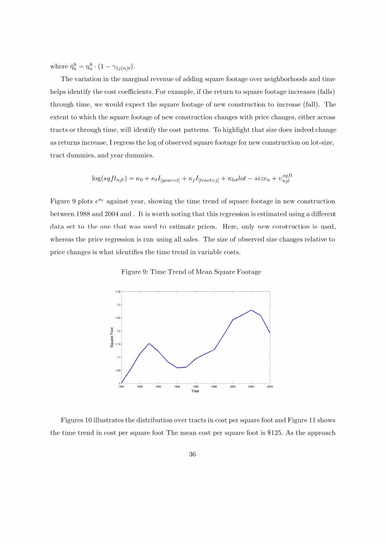
8/12/2019 Model of Housing Supply
http://slidepdf.com/reader/full/model-of-housing-supply 36/53
where ηhn = ηh
n · (1 − γ 1 j(n)t).
The variation in the marginal revenue of adding square footage over neighborhoods and time
helps identify the cost coefficients. For example, if the return to square footage increases (falls)through time, we would expect the square footage of new construction to increase (fall). The
extent to which the square footage of new construction changes with price changes, either across
tracts or through time, will identify the cost patterns. To highlight that size does indeed change
as returns increase, I regress the log of observed square footage for new construction on lot-size,
tract dummies, and year dummies.
log(sqftnjt ) = κ0 + κtI [year=t] + κ jI [tract= j] + κlotlot − sizen + υsqftnjt
Figure 9 plots eκt against year, showing the time trend of square footage in new construction
between 1988 and 2004 and . It is worth noting that this regression is estimated using a different
data set to the one that was used to estimate prices. Here, only new construction is used,
whereas the price regression is run using all sales. The size of observed size changes relative to
price changes is what identifies the time trend in variable costs.
Figure 9: Time Trend of Mean Square Footage
Figures 10 illustrates the distribution over tracts in cost per square foot and Figure 11 shows
the time trend in cost per square foot The mean cost per square foot is $125. As the approach
36

8/12/2019 Model of Housing Supply
http://slidepdf.com/reader/full/model-of-housing-supply 37/53
to identifying costs is different here from previous research, it is not completely straightforward
to compare results. Here, the costs include any costs that increase as house size increases. In
addition to raw building supplies and labor, this could also include any additional costs imposedby regulation or local opposition to building that increases with house size. As such, these costs
could be higher than costs estimated from physical costs alone. Gyourko and Saiz (2006) report
the average cost per square foot (of a 2000 f t2 house) in San Francisco in 2003 was $72 for an
economy quality house – higher costs apply to higher quality homes.47 The mean cost per square
foot in 2003 estimated here is $110. However, given the the “economy” quality in Gyourko and
Saiz (2006), the estimates do not appear to be that different.48
Figure 10: Distribution of the Cost per Square Foot
An important difference between the results here and the data used in Gyourko and Saiz
(2006) is that I allow cost per square foot to vary within a metropolitan area. While physical
construction costs for the same product are not expected to differ within the Bay Area, the
quality of house will vary from tract to tract. That is, neighborhoods can differ in two ways:
they may have different amenities but they also may have different prices because of the mean
quality of construction. Both factors drive price differences. For example, neighborhoods with
views of the Bay or which are close to employment centers will have higher prices, as will
47This figure was taken from R.S. Means Company cost data.48Wheaton and Simonton (2007) report costs for apartment and office buildings that are also quite similar.
37

8/12/2019 Model of Housing Supply
http://slidepdf.com/reader/full/model-of-housing-supply 38/53
Figure 11: Time Trend of the Cost per Square Foot
neighborhoods where it is common to use higher quality raw materials such as granite counter
tops. For construction costs, however, only the quality of construction matters. The underlying
assumption is that while the quality of square foot is homogenous within a tract, it can vary
across tracts. This added flexibility is a result of the fine level of geography at which I estimate
both price gradients and cost functions.
Finally, as shown in Figure 11, the time pattern of mean tract costs suggests that variable
costs are pro-cyclical and maybe falling slightly over time. It is somewhat surprising that costs
fall so sharply following a small downturn in prices and construction levels around 2000. The
volatility of variable costs is an interesting result as it is higher than that found in other work.
6.3 Dynamic Discrete Choice Results
6.3.1 Step One - Transition Probabilities and CCPs
The first step of the dynamic discrete choice estimation involves estimating transition probabil-
ities on costs and prices as well as reduced-form (flexible) conditional choice probabilities. As
the prices and costs are estimated at a fine level of geography, I estimate their transitions in
levels instead of first differences.49 The appendix provides tables of autoregressive coefficients
49Case and Shiller (1989) discuss the problems associated with first-differenced price estimates.
38

8/12/2019 Model of Housing Supply
http://slidepdf.com/reader/full/model-of-housing-supply 39/53
for prices and costs as well as an impulse response function showing the expected response of
prices to a one standard deviation positive shock. The results show similar patterns to those
estimated elsewhere in the literature. The coefficients on lagged levels imply similar qualitativeresults to Glaeser and Gyourko (2007), who use first differences. Both these results and those
found in Glaeser and Gyourko (2007) imply short run (one year) persistence of price shocks with
medium run (5 years) mean reversion.
The conditional choice probability estimation captures in a flexible way that the probability of
construction is increasing in prices, falling in costs, and differs significantly across neighborhoods.
6.3.2 Step Two - Structural Parameters
The remaining structural parameters, given the estimates of prices and variable costs from stages
one and two, are the discount parameter, β , the scale of the Type 1 extreme value error, σ, and
the neighborhood and year effects on fixed costs. The discount parameter, β is set at .95 and
the other parameters are estimated via maximum likelihood.
Table 3 in the appendix presents the results with the neighborhood effects suppressed. A
full set of neighborhood dummies were included and the omitted year was 1989. As the profit
function is measured in dollars, the scale of the extreme value error, σ is identified and was
estimated at $35,490. Using the properties of the Type 1 Extreme Value distribution, this yieldsan estimated standard deviation of the error equal to σ · π2/6 = $58, 385. Given the mean
($352,489) and standard deviation ($221,364) of observed house prices in the data, the size of
the error scale suggests the model fits the data quite well.
6.3.3 Fixed Costs – Cross-Section
The size of estimated fixed costs is quite high, with a mean of $284,180. However, it is important
to interpret the costs correctly. These are estimates of the costs that a randomly picked parcel
owner in a randomly picked time period would face from developing their land. Of greater
interest are the costs faced by those who actually engaged in construction. To get this figure, I
simply subtract the expectation of the logit error term conditional on a parcel being built. The
conditional expectation is $141,150. Subtracting the conditional expectation of the error from
39

8/12/2019 Model of Housing Supply
http://slidepdf.com/reader/full/model-of-housing-supply 40/53
the raw fixed cost estimates gives an estimate of the fixed costs incurred by those who developed
their parcels.
The fixed costs are allowed to vary at the PUMA level and the results show substantial cross-sectional variation. The fixed costs reflect any components of costs not captured by the variable
costs. As such, they reflect the physical costs of construction that do not vary with house size.
More interestingly, they also capture the regulatory environment. If we assume that the physical
construction component of fixed costs is fixed across PUMA, then the cross-sectional variation
reflects how the costs of regulation vary by area. If physical and regulatory costs are positively
correlated, the cross-sectional differences in fixed costs can be interpreted as upper bounds on
the differences in regulation. Figure 12 shows the adjusted fixed cost for each PUMA. Each
PUMA’s cost is calculated as the mean cost over time and the range of costs across PUMAs is
$81,710.50
Recent research, such as Glaeser, Gyourko, and Saks (2005) and Quigley and Raphael (2005)
has discussed the role of regulation in house price growth. Quigley (2006) and Kahn (2007) draw
attention to the possible role of existing residents in limiting housing supply and Ortalo-Magne
and Prat (2005) develops a theoretical political economy model, which models the incentives of
voting residents in determining new construction.51 To get an idea of how costs vary according
to PUMA characteristics and demographics, I can decompose the area fixed costs by regressing
fixed costs on PUMA characteristics. I therefore estimate δ j(n) = x j(n) + ξ j(n) by OLS.
Table 1 shows the results from these regressions with various combinations of regressors.
Costs are estimated for each of 46 PUMAs. The PUMA containing Oakland is an outlier is this
regression. Given the small number of observations, and the sensitivity of OLS to outliers, I
estimate regressions using a median regression using all 46 PUMAs, and using OLS with the
Oakland PUMA omitted. The partial correlations shown in Table 1 suggest that costs are
statistically significantly higher in high house price areas and areas with older houses. Costs are
higher, on average, in areas with lower household income and higher rates of home ownership.
50The area in the North-East of San Francisco is blank because of low numbers of single family residential sales.San Francisco International Airport is the other blank area.
51See Pope-Handy (2006) for a local realtor’s response to Quigley’s article in the Economist’s Voice. Therealtor disagreed with Quigley that local residents were blocking construction and suggested that Quigley was“too cynical.”
40

8/12/2019 Model of Housing Supply
http://slidepdf.com/reader/full/model-of-housing-supply 41/53
Figure 12: Geographic Distribution of Fixed Costs
Santa Clara
Marin
Alameda
Contra Costa
San Mateo
San Francisco
Fixed Costs
41730 - 50700
50701 - 56730
56731 - 63120
63121 - 72420
72421 - 76610
76611 - 85600
85601 - 89710
89711 - 123840
Race and education are found to be insignificant in predicting fixed costs. The effects for race
and education are relatively small and insignificant. Estimating the equation using OLS and
all 46 PUMAs gives similar results. The only substantial difference is that the coefficient on
ownership rates falls in size by approximately a half.
As the size of a PUMA is sufficiently large, there will be considerable heterogeneity in tract
characteristics and tract construction levels within each. Therefore, the regressions are more
suggestive than a true test of whether existing residents are blocking development. The regression
results reported here capture that costs are lower in parts of Contra Costa, Alameda, and Santa
Clara counties that are further from the central urban areas. These “newer” areas typically have
lower property age, lower house prices, and higher incomes. Future work will examine within-
PUMA variation to look at a more causal relationship between demographics and development
41

8/12/2019 Model of Housing Supply
http://slidepdf.com/reader/full/model-of-housing-supply 42/53
rates.
Table 1: Fixed Costs - Cross Section
F C j F C j F C j F C j% owner-occupied 598.34 520.52 549.09 449.96
[478.79] [113.26]** [242.49]* [222.35]*mean property age 669.28 820.76 864.34 879.76
[279.20]* [71.20]** [146.83]** [136.95]**mean income -0.8 -0.41 -0.62 -0.47
[0.48] [0.10]** [0.24]* [0.18]*mean house value 0.12 0.08 0.11 0.09
[0.07] [0.02]** [0.03]** [0.03]**% white 220.98 135.21
[195.01] [95.92]
% degree 345.01 91.9[409.16] [196.51]
Constant 127,681 140,814 129,706 138,988[34,315]** [8,362]** [17,887]** [16,553]**
Regression LAD LAD OLS OLSObservations 46 46 45 45R-squared 0.55 0.53 0.78 0.77
Standard errors in brackets. * significant at 5%; ** significant at 1%
6.3.4 Fixed Costs - Time Series
The other dimension of fixed costs are the estimates of the time effects. The year coefficients
by themselves are difficult to interpret. However, we can use the year coefficients combined
with the mean PUMA effect to get an estimate of the mean δ t − βE tδ t+1 for each year, where
the mean is taken over the PUMAs. These results are reported in Table 2. The year effects
suggest that fixed costs (or at least expectations about costs) are strongly pro-cyclical. For
example in 1993, costs are $32,280 higher than the discounted value of the expected costs in
1994. As prices boom at the end of the sample, this reverses. In 2002, parcel owners expect
costs to rise substantially – discounted expected costs for 2003 exceed 2002 costs by $36,682.
The cost changes are sufficiently high that in boom periods the expected discounted value of
next period’s costs significantly exceeds current period costs. This actually smooths construction
levels in a dynamic model and helps explain the observed construction volatility levels. The role
42
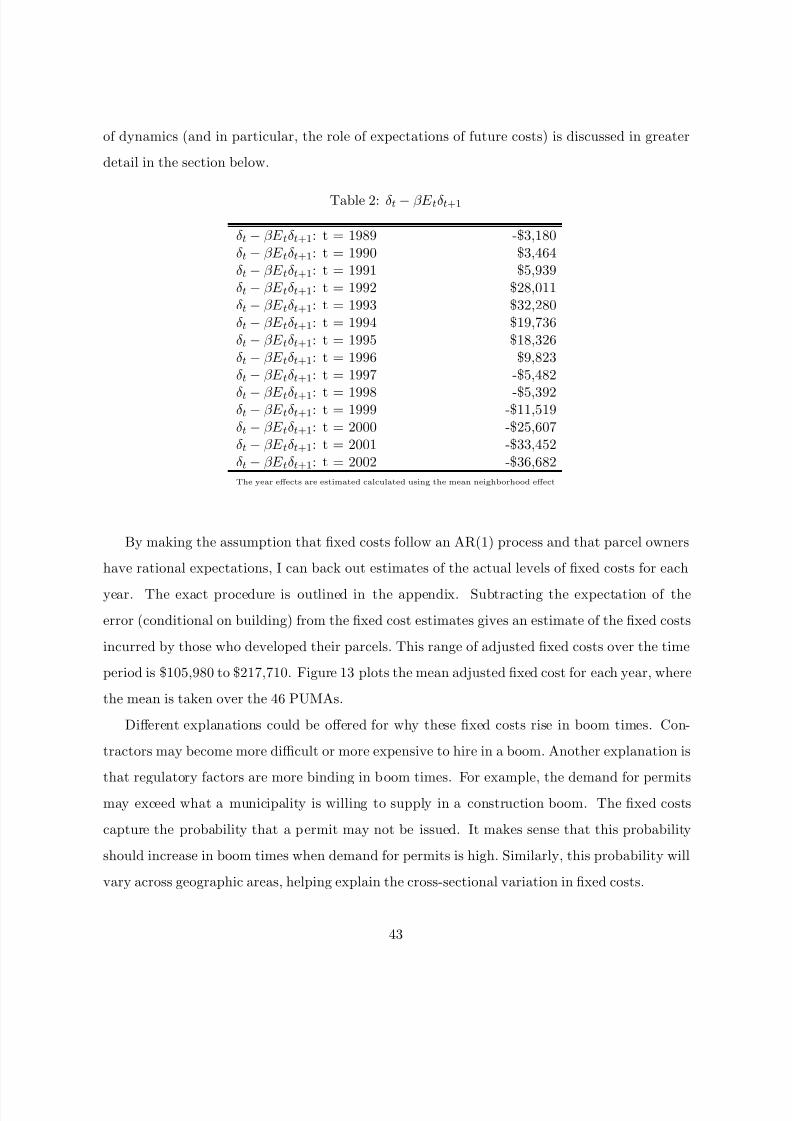
8/12/2019 Model of Housing Supply
http://slidepdf.com/reader/full/model-of-housing-supply 43/53
of dynamics (and in particular, the role of expectations of future costs) is discussed in greater
detail in the section below.
Table 2: δ t − βE tδ t+1
δ t − βE tδ t+1: t = 1989 -$3,180δ t − βE tδ t+1: t = 1990 $3,464δ t − βE tδ t+1: t = 1991 $5,939δ t − βE tδ t+1: t = 1992 $28,011δ t − βE tδ t+1: t = 1993 $32,280δ t − βE tδ t+1: t = 1994 $19,736δ t − βE tδ t+1: t = 1995 $18,326δ t − βE tδ t+1: t = 1996 $9,823δ t − βE tδ t+1: t = 1997 -$5,482
δ t − βE tδ t+1: t = 1998 -$5,392δ t − βE tδ t+1: t = 1999 -$11,519δ t − βE tδ t+1: t = 2000 -$25,607δ t − βE tδ t+1: t = 2001 -$33,452δ t − βE tδ t+1: t = 2002 -$36,682
The year effects are estimated calculated using the mean neighborhood effect
By making the assumption that fixed costs follow an AR(1) process and that parcel owners
have rational expectations, I can back out estimates of the actual levels of fixed costs for each
year. The exact procedure is outlined in the appendix. Subtracting the expectation of the
error (conditional on building) from the fixed cost estimates gives an estimate of the fixed costs
incurred by those who developed their parcels. This range of adjusted fixed costs over the time
period is $105,980 to $217,710. Figure 13 plots the mean adjusted fixed cost for each year, where
the mean is taken over the 46 PUMAs.
Different explanations could be offered for why these fixed costs rise in boom times. Con-
tractors may become more difficult or more expensive to hire in a boom. Another explanation is
that regulatory factors are more binding in boom times. For example, the demand for permits
may exceed what a municipality is willing to supply in a construction boom. The fixed costs
capture the probability that a permit may not be issued. It makes sense that this probability
should increase in boom times when demand for permits is high. Similarly, this probability will
vary across geographic areas, helping explain the cross-sectional variation in fixed costs.
43

8/12/2019 Model of Housing Supply
http://slidepdf.com/reader/full/model-of-housing-supply 44/53
Figure 13: Time Trend of Fixed Costs
7 Implications of Dynamic Behavior
With observed historical patterns of price and cost cycles and trends, it is clear that a dynamic
model is necessary to understand the primitives that drive housing supply. Given the focus in
the literature on prices, a naıve model which ignored expectations about cost patterns would
predict very large levels of construction volatility. In the extreme case where prices were perfectly
predictable, discounting of future profits is low, and costs were constant, we would expect to
see construction only at the peak of prices. In reality, a sizeable amount of construction occurs
prior to the peak. Various explanations for this observed pattern could be offered: prices are
not predictable, parcels owners heavily discount future profits, the time to build is large, and
costs are pro-cyclical. I can examine these different accounts and, using the estimates of the
structural model, attribute the primary role to pro-cyclical costs.
If the time required to build was sufficiently long relative to the typical cycle of prices, it
would make sense for parcel owners to begin building early in the price cycle. However, empiricalevidence does not support this. According to figures from the Census of Construction, 54% of
construction in the West Census Region is completed within six months and 91% is completed
within twelve months.52 These time periods are short when compared with the length of the
52See Coulson (1999) for an analysis of the relationship between starts, completions, and housing inventory.
44

8/12/2019 Model of Housing Supply
http://slidepdf.com/reader/full/model-of-housing-supply 45/53
price cycle. The expected length of price growth is considerably longer, with prices usually only
mean-reverting 5 years after a price shock.53
The effects of the discount factor and price expectations are easier to rule out as they arenot estimated directly in the dynamic discrete choice estimation. The discount factor, β , is
set at .95, a level consistent with the literature. The transition probabilities are estimated
outside of the final estimation routine and are estimated assuming parcel owners have rational
expectations. The only factor estimated in the final step of estimation is the cost consideration
term, δ t − βE tδ t+1. Given the estimates of δ t − βE tδ t+1, it is clear that without including cost
considerations, the model would underpredict construction during the boom period beginning
in the late 1990s. These coefficients are significantly negative in boom times, indicating that
parcel owners believe that delaying construction will result in higher costs in the future. The
implication of these results is that rising costs discourage parcel owners from only building at the
peak and that cost trends and forward-looking behavior dampen construction volatility. Only by
including the fixed cost patterns can the observed level of volatility be explained – the discount
factor and prices are not enough.
This can be further illustrated using a counterfactual simulation. In the counterfactual
simulation, I consider what would happen if parcel owners had adaptive expectations about the
future cost environment. That is, E tδ
t+1 = δ
t. To do this, I use the estimates of δ
t obtained from
the estimation along with the fixed discount factor, β , and the price transitions taken directly
from the data. I then fully solve the model and predict construction in each period. I can then
compare the path of the simulated construction with the actual path.54
Figure 14 shows how the counterfactual construction levels compare with actual levels of
construction. The first panel shows the number of observed and predicted residences built. The
lower panel shows the observed and predicted portion of available parcels that were developed.
During the downturn in the early 1990s, construction levels are actually higher with adaptive
expectations. This is because in the counterfactual scenario parcel owners are not taking into
account that costs are falling. However, the interesting pattern begins around 1996. This roughly
53In the data used here, prices began to increase in the mid 1990s and continued to rise though the end of thesample period in 2004. Some areas experienced small reductions in real prices briefly in 2001.
54As the estimation routine effectively included time fixed effects the predicted construction trends from thetrue model will fit perfectly the true trends at the Bay Area level.
45

8/12/2019 Model of Housing Supply
http://slidepdf.com/reader/full/model-of-housing-supply 46/53
Figure 14: Counterfactual - Adaptive Expectations
corresponds to the beginning of the upturn in prices in the Bay Area. As prices begin to rise, so
do expectations about future prices in both scenarios. However, in the counterfactual scenario,
parcel owners do not take into account that costs will also rise in the future. Without the cost
deterrent to waiting for a price peak, construction falls as owners delay construction waiting
for the peak. Unfortunately for illustrative purposes, the time horizon of the data does not
include a peak following this rapid price appreciation. However, if it did, we would expect to
see construction in the counterfactual simulation to shoot up around the peak as there is a
build-up of parcel owners who delayed construction in anticipation of such a peak. In contrast
construction levels in the observed data increase gradually as prices increase. The construction
early in the price boom is caused by the expectations of future cost increases.
This counterfactual experiment highlights the role of costs and cost expectations in dampen-
ing construction volatility. When parcel owners are only forward looking with respect to prices
they will try and delay construction until a price peak. In reality, however, expectations about
future cost increases flatten out the time profile of construction.
46

8/12/2019 Model of Housing Supply
http://slidepdf.com/reader/full/model-of-housing-supply 47/53
8 Conclusion
The importance of the housing market has been well-documented, but the literature on housing
supply is surprisingly small. Short-run volatility in both price and construction levels has large
welfare implications – in the case of prices, because of their effect on a typical household’s asset
portfolio and, in the case of construction, because of its employment effects. Understanding
the way that economic primitives influence the individual behavior is crucial in explaining the
aggregate patterns of construction and prices observed in macro data.
To that end, I estimate a model of parcel owners’ development decisions. By combing the
static continuous choice of what size to build with the dynamic discrete choice of when to build,
I estimate the parameters of the profit function at a fine level of geography and still retaincomputational tractability. By using a multi-step estimator, I incorporate a large descriptive
state space and estimate prices and variable costs at the Census tract level. Additionally, the
estimation routine allows for time-varying parameters. Prices and variable costs are not sufficient
for understanding the parcel owner’s decision process and therefore fixed costs (which capture
the overall cost environment) are estimated.
The price results suggest that changes in housing prices are driven by changes in the value of
the right-to-build. Cost results indicate that both variable costs and fixed costs are strongly pro-
cyclical. There is also substantial variation in the fixed costs of building across neighborhoods,
with high home ownership rates predicting higher costs. Forward-looking behavior is found to be
very important in trying to understand construction volatility. Parcel owners look to the future
about both prices and costs when deciding when to build. Using the fact that prices are partially
predictable, this paper structurally incorporates these expectations into a model of supply. The
literature on cost trends is more sparse. Here, the results suggest that trends in the overall cost
environment are pro-cyclical and that forward looking dynamic behavior, with regard to these
costs, is crucial in understanding and explaining observed construction patterns.
47

8/12/2019 Model of Housing Supply
http://slidepdf.com/reader/full/model-of-housing-supply 48/53
References
Aguirregabiria, V., and P. Mira (2002): “Swapping the nested fixed point algorithm: a
class of estimators for discrete Markov decision models,” Econometrica , 70(4), 1519–1543.
Arcidiacono, P., and R. A. Miller (2008): “CCP Estimation of Dynamic Discrete Choice
Models with Unobserved Heterogeneity,” mimeo, Duke University.
Bailey, M., R. Muth, and H. Nourse (1963): “A Regression Method for Real Estate Price
Index Construction,” Journal of the American Statistical Association , 58, 933–942.
Bajari, P., C. L. Benkard, and J. Levin (2007): “Estimating Dynamic Models of Imperfect
Competition,” Econometrica , 75(5), 1331–1370.
Bayer, P., R. McMillan, A. Murphy, and C. Timmins (2007): “A Dynamic Model of
Housing Demand,” working paper, Duke University.
Berry, S. (1994): “Estimating Discrete Choice Models of Product Differation,” Rand Journal
of Economics , 25, 242–262.
Berry, S., J. Levinsohn, and A. Pakes (1995): “Automobile Prices in Market Equilibrium,”
Econometrica , 63, 841–890.
Case, K., and R. Shiller (1987): “Prices of Single Family Homes Since 1970: New Indexes
for Four Cities,” New England Economic Review , pp. 45–56.
(1989): “The Efficiency of the Market for Single-Family Homes,” American Economic
Review , 79(1), 125–137.
Cheshire, P., and S. Sheppard (1998): “Estimating the Demand for Housing, Land, and
Neighbourhood Characteristics,” Oxford Bulletin of Economics and Statistics , 60(3), 357–382.
Clapham, E., P. Englund, J. M. Quigley, and C. L. Redfearn (2006): “Revisiting the
past and settling the score: Index revision for house price derivatives,” Real Estate Economics ,
34(2), 275–302.
Coulson, N. (1999): “Housing Inventory and Completion,” The Journal of Real Estate Finance
and Economics , 18(1), 89–105.
Cropper, M. L., L. B. Deck, and K. E. McConnell (1988): “On the Choice of Funtional
Form for Hedonic Price Functions,” The Review of Economics and Statistics , 70(4), 668–675.
DiPasquale, D. (1999): “Why Don’t We Know More About Hosuing Supply?,” Journal of
Real Estate Finance and Economics , 18(1), 9–23.
48

8/12/2019 Model of Housing Supply
http://slidepdf.com/reader/full/model-of-housing-supply 49/53
DiPasquale, D., and W. C. Wheaton (1994): “Housing Market Dynamics and the Future
of Housing Prices,” Journal of Urban Economics , 31(3), 337–359.
Epple, D., B. Gordon, and H. Sieg (2007): “A New Approach to Estimating the Production
Function for Housing,” Working Paper.
Follain, J. R. (1979): “The Price Elasticity of the Long-Run Supply of New Housing Con-
struction,” Land Economics , 55(2), 190–199.
Glaeser, E., and J. Gyourko (2007): “Housing Dynamics,” mimeo.
Glaeser, E. L., J. Gyourko, and R. E. Saks (2005): “Why Have Housing Prices Gone
Up?,” H.I.E.R. Discussion Paper 2061.
(2006): “Urban Growth and Housing Supply,” Journal of Economic Geography , 6,
71–89.
Gowrisankaran, G., and M. Rysman (2006): “Dynamics of Consumer Demand for New
Durable Goods,” mimeo.
Gyourko, J., C. Mayer, and T. Sinai (2006): “Superstar Cities,” NBER Working Paper
12355.
Gyourko, J., and A. Saiz (2006): “Construction Costs and the Supply of Housing Structure,”
Journal of Regional Science , 46(4), 661–680.
Hotz, V. J., and R. A. Miller (1993): “Conditional Choice Probabilities and the Estimation
of Dynamic Models,” Review of Economic Studies , 60, 497–529.
Kahn, M. (2007): “Environmentalism as a Determinant of Housing Supply Regulation,” mimeo.
Mayer, C., and C. T. Somerville (2000): “Residential Construction: Using the Urban
Growth Model to Estimate Hosuing Supply,” Journal of Urban Economics , 48, 85–109.
Meese, R. A., and N. E. Wallace (1997): “The Construction of Residential Housing Price In-
dices: A Comparison of Repeat Sales, Hedonic-Regression, and Hybrid Approaches,” Journal
of Real Estate Finance and Economics , 14, 51–73.
Muth, R. (1960): “The Demand for Non-Farm Housing,” in The Demand for Durable Goods ,
ed. by A. C. Harberger. University of Chicago Press.
Newey, W., and D. McFadden (1994): “Large Sample Estimation and Hypothesis Testing,”
Handbook of Econometrics , 4, 2111–2245.
Ortalo-Magne, F., and A. Prat (2005): “The Political Economy of Housing Supply,” mimeo.
49

8/12/2019 Model of Housing Supply
http://slidepdf.com/reader/full/model-of-housing-supply 50/53
Pakes, A., M. Ostrovsky, and S. Berry (2007): “Simple estimators for the parameters
of discrete dynamic games (with entry/exit examples),” The RAND Journal of Economics ,
38(2), 373–399.
Pope-Handy, M. E. (2006): “Letter: Is Professor Quigley Too Cynical?,” The Economist’s
Voice , 3(9), Article 5.
Poterba, J. M. (1984): “Tax Subsidies to Owner Occupied Housing: An Asset Market Ap-
proach,” Quarterly Journal of Economics , 99(4), 729–52.
Quigley, J., and S. Raphael (2005): “Regulation and the High Cost of Housing in California,”
American Economic Review , 95(2), 323–328, AEA Papers and Proceedings.
Quigley, J. M. (2006): “Froth in the Silicon Valley Housing Market?,” The Economist’s Voice ,
3(5), Article 1.
Roback, J. (1982): “Wages, Rents, and the Quality of Life,” Journal of Political Economy ,
90(6), 1257–1278.
Rust, J. (1987): “Optimal Replacement of GMC Bus Engines: An Empirical Model of Harold
Zurcher,” Econometrica , 55(5), 999–1033.
(1994): “Structural Estimation of Markov Decision Processes,” in Handbook of Econo-
metrics , ed. by R. Engle, and D. McFadden, vol. 4. New York: North Holland.
Schiraldi, P. (2006): “Automobile Replacement: A Dynamic Structural Approach,” mimeo,
Boston University.
Somerville, C. T. (1999): “Residential Construction Costs and the Supply of New Housing:
Endogeneity and Bias in Construction Cost Indexes,” Journal of Real Estate Finance and
Economics , 18(1), 43–62.
Stover, M. E. (1986): “The Price Elasticity of the Supply of Single-Family Detached Urban
Housing,” Journal of Urban Economics , 20(3), 331–340.
Topel, R., and S. Rosen (1988): “Housing Investment in the United States,” Journal of
Political Economy , 96(4), 718–740.
Tracy, J., H. Schneider, and S. Chan (1999): “Are Stocks Overtaking Real Estate inHousehold Portfolios?,” Current Issues in Economics and Finance , 5(5), 1–6.
Wheaton, W. C., and W. E. Simonton (2007): “The Secular and Cyclic Behavior of ‘True’
Construction Costs,” The Journal of Real Estate Research , 29(1), 1–25.
50

8/12/2019 Model of Housing Supply
http://slidepdf.com/reader/full/model-of-housing-supply 51/53
9 Appendix
Further Estimation Details
Two options are available for estimating δ t. The first option would be to assume a transition
probability for δ t – for example, an AR(1) specification – and use this within the estimation
routine. This would involve guessing a parameter vector δ t, estimating (via OLS) first order
autoregressive process transition probabilities, and then evaluating the likelihood using both the
chosen parameters and the expected future costs implied by those parameters. This approach
would be most similar to Gowrisankaran and Rysman (2006).
The alternative which is used here is to simply estimate year effects to get δ t − βE tδ t+1.Assuming that transition probabilities are given by an AR(1) process yields a set of unique
values for δ t for a given set of autoregressive coefficients. The autoregressive coefficients which
minimize the sum of square residuals using the resulting values for δ t are chosen.
To summarize, the steps are outlined below. Using the vector of estimates of δ t − βE tδ t+1
1) Guess values for α in the equation δ t+1 = α0 + α1δ t + α2xt + υt.
2) Solve for δ t using α and δ t − βE tδ t+1.
3) Solve for residuals from the equation υt = δ t+1 − (α0 + α1δ t + α2xt), given x, δ t and α.
4) Calculate the sum of squared residuals, ssrυ = T t=1 υ2
t .
5) Choose α to minimize sum of square residuals, ssrυ.
51

8/12/2019 Model of Housing Supply
http://slidepdf.com/reader/full/model-of-housing-supply 52/53
Transition Probabilities
EP nt = φ0,j +L
l=1
φ1,lEP nt−l + φ2lot − sizen + φ3t + εEP nt
Table 3: Transition Probabilities: Price
Coefficient Standard Error
φ1,1 2.0460 .0868φ1,2 -1.9206 .1680φ1,3 1.4173 .1819φ1,4 -1.1551 .1985φ1,5 0.9762 .2080
φ1,6 -0.6875 .1471φ1,7 0.2784 .0499lot − size 3.884e-6 6.3162e-7time .0070 .0015R2 .9793
Area constants, φ0,j , are suppressed. All coefficients significant at 1% level
Figure 15: Impulse Response Function: One Standard Deviation Increase in Prices
52

8/12/2019 Model of Housing Supply
http://slidepdf.com/reader/full/model-of-housing-supply 53/53
Additional Results
Table 4: Dynamic Discrete Choice - Structural Parameters
Coefficient Standard Error
1/σ .0000282 .000002271990 6638 53511991 9111 54551992 31162 73511993 35428 132861994 22929 100911995 22907 100071996 12993 77081997 -2302 80461998 -2210 56741999 -8333 51472000 -22409 47632001 -30250 75662002 -33480 7613PUMA Dummies yesObservations 1210478Likelihood -255450