Model Documentation Report: Industrial Demand Module of the National Energy Modeling ...2014).pdf · 2014-08-06 · August 2014 U.S. Energy Information Administration | Model Documentation

Model Documentation Report: Industrial Demand Module of the National Energy Modeling System

August 2014

Independent Statistics & Analysis

www.eia.gov

U.S. Department of Energy

Washington, DC 20585

U.S. Energy Information Administration | Model Documentation Report: Industrial Demand Module of the National Energy Modeling System i

This report was prepared by the U.S. Energy Information Administration (EIA), the statistical and analytical agency within the U.S. Department of Energy. By law, EIA’s data, analyses, and forecasts are independent of approval by any other officer or employee of the United States Government. The views in this report therefore should not be construed as representing those of the Department of Energy or other Federal agencies.

August 2014

U.S. Energy Information Administration | Model Documentation Report: Industrial Demand Module of the National Energy Modeling System 1

Table of Contents 1. Introduction .............................................................................................................................................. 5

Model summary ....................................................................................................................................... 5

Archival media ......................................................................................................................................... 6

Model contact .......................................................................................................................................... 6

Organization of this report ...................................................................................................................... 6

2. Model Purpose .......................................................................................................................................... 8

Interaction with other NEMS modules .................................................................................................. 10

3. Model Rationale ...................................................................................................................................... 11

Theoretical approach ............................................................................................................................. 11

Modeling approach ................................................................................................................................ 11

Fundamental assumptions .................................................................................................................... 12

Industry disaggregation ......................................................................................................................... 14

Energy sources modeled ........................................................................................................................ 14

Key computations .................................................................................................................................. 16

Buildings component UEC ..................................................................................................................... 16

Process and assembly component UEC ................................................................................................. 16

Energy-intensive manufacturing industries ........................................................................................... 17

Non-energy-intensive manufacturing industries ................................................................................... 31

Non-manufacturing industries ............................................................................................................... 32

Agricultural submodule ......................................................................................................................... 33

Mining submodule ................................................................................................................................. 34

Construction submodule ....................................................................................................................... 34

Boiler, steam, cogeneration component ............................................................................................... 39

Additional model assumptions .............................................................................................................. 43

Renewable fuels ..................................................................................................................................... 44

4. Model Structure ...................................................................................................................................... 45

Outline of model .................................................................................................................................... 45

Subroutines and equations .................................................................................................................... 47

Factor indices for vehicles and equipment ............................................................................................ 57

Factor indices ......................................................................................................................................... 61

August 2014


Metal/non-metal split ............................................................................................................................ 69

Technology Choice Options ................................................................................................................... 75

CALBSC .......................................................................................................................................... 145

Appendix A. Model Abstract ..................................................................................................................... 146

Model name: ........................................................................................................................................ 146

Model acronym: ................................................................................................................................... 146

Description: .......................................................................................................................................... 146

Purpose of the model: ......................................................................................................................... 146

Most recent model update: ................................................................................................................. 146

Part of another model: ........................................................................................................................ 146

Model interfaces: ................................................................................................................................. 146

Official model representatives: ........................................................................................................... 146

Documentation: ................................................................................................................................... 147

Archive media and installation manual(s): .......................................................................................... 147

Energy system described: .................................................................................................................... 147

Coverage: ............................................................................................................................................. 147

Modeling features: .............................................................................................................................. 147

Non-DOE input sources: ...................................................................................................................... 147

DOE input sources: .............................................................................................................................. 147

Computing environment: .................................................................................................................... 148

Appendix B. Data Inputs and input variables ............................................................................................ 149

Industrial demand module exogenous input files ............................................................................... 149

Industrial demand module hardcoded data ........................................................................................ 164

Appendix C. Descriptions of Major Industrial Groups and Selected Industries ........................................ 168

Appendix D. Bibliography .......................................................................................................................... 176

August 2014


Tables Table 1. Census regions and Census divisions .............................................................................................. 6 Table 2. Industry categories, NAICS codes, and IDM industry codes ........................................................ 15 Table 3. Chemical products in the bulk chemical industry model .............................................................. 21 Table 4. Motor sizes used in motor stock model ........................................................................................ 37 Table 5. Building weights for TPC index by fuel .......................................................................................... 54 Table 6. Total cost of selected power, fuels, and lubricants, 2007 ............................................................ 55 Table 7. Gasoline/distillate volume allocation ............................................................................................ 56 Table 8. Regional share of employees, by functional group ....................................................................... 56 Table 9. Construction UEC weights by region: -variable weight_con ........................................................ 57 Table 10. Functional groups and vehicles ................................................................................................... 58 Table 11. Fuel use weights for buildings ..................................................................................................... 59 Table 12. Relative contribution to total TPC, vehicles and other equipment............................................. 59 Table 13. Energy weights for mining equipment ........................................................................................ 62 Table 14. Census region and coal region mapping ..................................................................................... 63 Table 15. TPC equipment component weights by region ........................................................................... 64 Table 16. Relative difficulty of extraction of oil and gas ............................................................................. 65 Table 17. OGSM and Census region mapping ............................................................................................. 66 Table 18. TPC factor weights by fuel (TPC_Fac_Wt) ................................................................................... 68 Table 19. Metal and nonmetal shares by Census region ............................................................................ 69 Table 20. Electric equipment weights ......................................................................................................... 71 Table 21. Non-electric equipment weights (Metals and non-metals) ........................................................ 71 Table 22. TPC equipment component weights by region ........................................................................... 72 Table 23. Major U.S. glass industry segments and typical products .......................................................... 73 Table 24. Flat glass technology choice ........................................................................................................ 75 Table 25. Container glass technology choice .............................................................................................. 76 Table 26. Blown glass technology choice .................................................................................................... 76 Table 27. Fiber glass technology choice ...................................................................................................... 77 Table 28. Initial allocation of cement kiln burners ..................................................................................... 95 Table 29. Initial allocations of process grinders ......................................................................................... 97 Table 30. Initial allocation of lime kilns .................................................................................................... 101 Table 31. Characteristics of lime kilns ....................................................................................................... 102 Table 32. Aluminum electrolysis technologies using hall-héroult process ............................................... 108 Table 33. Regression parameters for primary and secondary aluminum production projections ........... 110 Table 34. Boiler efficiency by fuel ............................................................................................................. 133 Table 35. Index price premiums for boiler fuel share selection ............................................................... 145

August 2014


Appendix B Tables Table B-1. Input files ................................................................................................................................. 149 Table B-2. Census Regions and Divisions .................................................................................................. 150 Table B-3. Industry categories, NAICS codes and IDM industry codes ..................................................... 150 Table B-4. INDBEU.txt inputs .................................................................................................................... 151 Table B-5. Cogeneration data ................................................................................................................... 152 Table B-6. Subroutine IRHEADER, IRBSCBYP and IRSTEPBYP input data ................................................. 154 Table B-7. INDRUN.txt input variables ...................................................................................................... 156 Table B-8. ITBSHR.txt input variables ........................................................................................................ 157 Table B-9. INDSTEO input data ................................................................................................................. 158 Table B-10. PRODFLOW steps and reporting groups ................................................................................ 159 Table B-11. Data inputs for indmotor.xml ................................................................................................ 160 Table B-12. EXSTCAP.txt & PLANCAP.txt input data ................................................................................. 163 Table B-13. IDM hardcoded data .............................................................................................................. 164

Figures Figure 1. Industrial Demand Module interactions within NEMS .................................................................. 8 Figure 2. Industrial Demand Module structure .......................................................................................... 13 Figure 3. Food industry end uses ................................................................................................................ 18 Figure 4. Paper manufacturing industry process flow ................................................................................ 19 Figure 5. Bulk chemical industry end uses .................................................................................................. 22 Figure 6. Glass industry process flow .......................................................................................................... 24 Figure 7. Cement industry process flow ..................................................................................................... 26 Figure 8. Lime industry process flow .......................................................................................................... 27 Figure 9. Iron and steel industry process flow ............................................................................................ 29 Figure 10. Aluminum industry process flow ............................................................................................... 31 Figure 11. Flow diagram of module solution .............................................................................................. 45 Figure 12. AEO Oil and Gas Supply Regions ................................................................................................ 66 Figure 13. Subroutine Execution for the Glass Submodule ........................................................................ 74 Figure 14. Cement industry detailed process flow ..................................................................................... 85 Figure 15. Cement submodule process steps ............................................................................................. 86 Figure 16. Survival function for new cement capacity ................................................................................ 89

August 2014


1. Introduction This report documents the objectives and analytical approach of the National Energy Modeling System (NEMS) Industrial Demand Module (IDM). The report catalogues and describes model assumptions, computational methodology, parameter estimation techniques, and model source code.

This document serves three purposes. First, it is a reference document providing a detailed description of the NEMS Industrial Demand Module for model analysts, users, and the public. Second, this report meets the legal requirement of the U.S. Energy Information Administration (EIA) to provide adequate documentation in support of its models (Public Law 94-385, section 57.b2). Third, it facilitates continuity in model development by providing documentation from which energy analysts can undertake model enhancements, data updates, and parameter refinements in future projects.

Model summary The NEMS Industrial Demand Module is a dynamic accounting model, bringing together disparate industries and uses of energy in those industries, and putting them together in an understandable and cohesive framework. The IDM generates long-term (up to the year 2040) projections of industrial sector energy demand as a component of the integrated NEMS. From NEMS, the IDM receives fuel prices, employment data, and the value of industrial shipments.

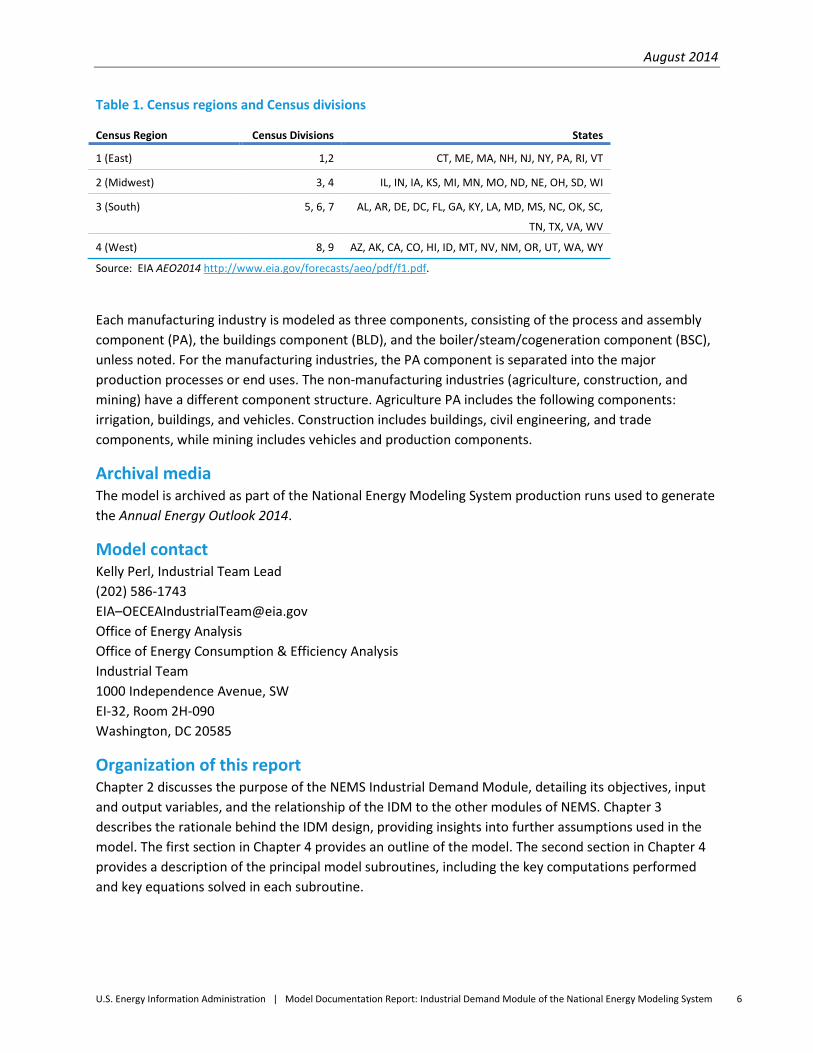
The NEMS Industrial Demand Module estimates energy consumption by energy source (fuels and feedstocks) for 15 manufacturing and 6 non-manufacturing industries. The manufacturing industries are classified as energy-intensive manufacturing industries and non-energy-intensive manufacturing industries. The manufacturing industries are modeled through the use of detailed process flows or end-use accounting procedures. The energy-intensive bulk chemicals industry is subdivided into four components, each with individual detailed process flows. The non-manufacturing industries are represented in less detail. The IDM projects energy consumption at the Census Region level; energy consumption at the Census Division level is allocated by using data from the State Energy Data System (SEDS) for 2011.1 The national-level values reported in the Annual Energy Review 2010 2 were allocated to the Census Divisions, also using the SEDS 2011 data.3 The four Census Regions are divided into nine Census Divisions and are listed in Table 1. They are also mapped in the Annual Energy Outlook 2014 (AEO2014).4

1 U.S. Energy Information Administration, State Energy Data System Report 2009, issued June 30, 2011, http://www.eia.gov/state/seds/. 2 U.S. Energy Information Administration, Annual Energy Review 2010, DOE/EIA-384(2010), October 2011, http://www.eia.gov/totalenergy/data/annual/. 3 U.S. Energy Information Administration, State Energy Data System Report 2009, http://www.eia.gov/state/seds/ 4 U.S. Energy Information Administration, Annual Energy Outlook 2014, pp. F-1–F-2. http://www.eia.gov/forecasts/aeo/pdf/f1.pdf.

http://www.eia.gov/state/seds/

http://www.eia.gov/totalenergy/data/annual/


http://www.eia.gov/forecasts/aeo/pdf/f1.pdf

August 2014


Table 1. Census regions and Census divisions

Census Region Census Divisions States 1 (East) 1,2 CT, ME, MA, NH, NJ, NY, PA, RI, VT

2 (Midwest) 3, 4 IL, IN, IA, KS, MI, MN, MO, ND, NE, OH, SD, WI

3 (South) 5, 6, 7 AL, AR, DE, DC, FL, GA, KY, LA, MD, MS, NC, OK, SC,

TN, TX, VA, WV

4 (West) 8, 9 AZ, AK, CA, CO, HI, ID, MT, NV, NM, OR, UT, WA, WY

Source: EIA AEO2014 http://www.eia.gov/forecasts/aeo/pdf/f1.pdf.

Each manufacturing industry is modeled as three components, consisting of the process and assembly component (PA), the buildings component (BLD), and the boiler/steam/cogeneration component (BSC), unless noted. For the manufacturing industries, the PA component is separated into the major production processes or end uses. The non-manufacturing industries (agriculture, construction, and mining) have a different component structure. Agriculture PA includes the following components: irrigation, buildings, and vehicles. Construction includes buildings, civil engineering, and trade components, while mining includes vehicles and production components.

Archival media The model is archived as part of the National Energy Modeling System production runs used to generate the Annual Energy Outlook 2014.

Model contact Kelly Perl, Industrial Team Lead (202) 586-1743 EIA–[email protected] Office of Energy Analysis Office of Energy Consumption & Efficiency Analysis Industrial Team 1000 Independence Avenue, SW EI-32, Room 2H-090 Washington, DC 20585

Organization of this report Chapter 2 discusses the purpose of the NEMS Industrial Demand Module, detailing its objectives, input and output variables, and the relationship of the IDM to the other modules of NEMS. Chapter 3 describes the rationale behind the IDM design, providing insights into further assumptions used in the model. The first section in Chapter 4 provides an outline of the model. The second section in Chapter 4 provides a description of the principal model subroutines, including the key computations performed and key equations solved in each subroutine.

http://www.eia.gov/forecasts/aeo/pdf/f1.pdf

August 2014


The Appendices to this report provide supporting documentation for the IDM. Appendix A is the model abstract. Appendix B lists the input data for AEO2014. Appendix C provides industrial group descriptions. Appendix D is a bibliography of data sources and background materials used in model development.

August 2014


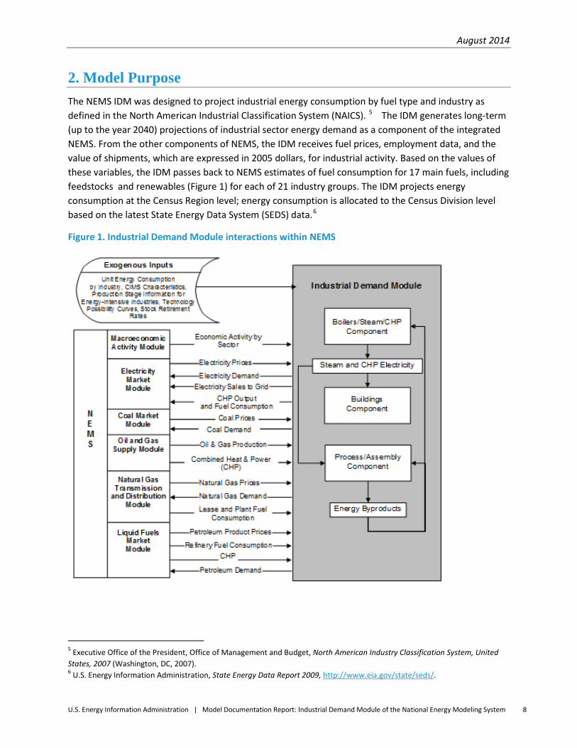
2. Model Purpose The NEMS IDM was designed to project industrial energy consumption by fuel type and industry as defined in the North American Industrial Classification System (NAICS). 5 The IDM generates long-term (up to the year 2040) projections of industrial sector energy demand as a component of the integrated NEMS. From the other components of NEMS, the IDM receives fuel prices, employment data, and the value of shipments, which are expressed in 2005 dollars, for industrial activity. Based on the values of these variables, the IDM passes back to NEMS estimates of fuel consumption for 17 main fuels, including feedstocks and renewables (Figure 1) for each of 21 industry groups. The IDM projects energy consumption at the Census Region level; energy consumption is allocated to the Census Division level based on the latest State Energy Data System (SEDS) data.6

Figure 1. Industrial Demand Module interactions within NEMS

5 Executive Office of the President, Office of Management and Budget, North American Industry Classification System, United States, 2007 (Washington, DC, 2007). 6 U.S. Energy Information Administration, State Energy Data Report 2009, http://www.eia.gov/state/seds/.


August 2014


The IDM is an annual energy model; as such, it does not project seasonal or daily variations in fuel demand or fuel prices. The model was designed primarily for use in applications such as the Annual Energy Outlook (AEO) and other analyses of long-term energy-economy interactions.

The model can also be used to examine various policy, environmental, and regulatory initiatives. For example, energy consumption per dollar of shipments is, in part, a function of energy prices. Therefore, the effect on industrial energy consumption of policies that change relative fuel prices can be analyzed endogenously in the model.

The IDM can also endogenously analyze specific technology programs or energy standards. The model distinguishes among the energy-intensive manufacturing industries, the non-energy-intensive manufacturing industries, and the non-manufacturing industries. Variation in the level of representational detail, and other details of IDM model structure, affect the suitability of the model for specific contexts.

A process flow approach, represented by the major production processes or end uses, is used to model the manufacturing industries. This approach provides considerable detail about how energy is consumed in a particular industry. The IDM uses “technology bundles” to characterize global technological change. These bundles are defined for each production process step for five of the manufacturing industries, for each end use in the remaining manufacturing industry groups, and for whole industries in the non-manufacturing sub-sector. The industries defined by process steps are pulp and paper, glass, cement and lime, iron and steel, and aluminum. The industries defined by end use are food, bulk chemicals, metal-based durables, and the balance of manufacturing.

The Unit Energy Consumption (UEC), a key indicator of energy intensity used in IDM, is defined as the energy use per ton of throughput at a process step or as energy use per dollar of shipments for the end-use industries. The “Existing UEC” is the current average installed intensity as of 2010. The “New 2010 UEC” is the intensity expected to prevail for a new, greenfield 7 installation in 2010. Similarly, the “New 2040 UEC” is the intensity expected to prevail for a new, greenfield installation in 2040. For intervening years, the intensity is interpolated.

A more detailed approach to modeling the process flow of energy intensive manufacturing industries is being incorporated into the IDM over a period of several years. For AEO2014, the IDM adopted this approach for the aluminum, cement and lime, and glass industries. Rather than a single point UEC value for process and assembly, the new approach represents distinct process steps within an industry. Within these steps are several technology options with their unique UECs, which, when aggregated, represent a means to link technology improvements with an overall UEC. The more detailed submodules are derived from the Consolidated Impacts Modeling System (CIMS) and other data sources.8 CIMS is an engineering-economic model based on a similar model developed for the Canadian economy by Energy and Materials Group at Simon Fraser University. Parts of CIMS are also based on the Industrial Sector

7 Denotes an investment where no previous investment existed. 8 Portland Cement Association and U.S. Department of the Interior, U.S. Geological Survey.

August 2014


Technology Use Model (ISTUM), developed by Pacific Northwest National Laboratory (PNNL) for the U.S. Department of Energy (DOE) in the 1980s.9

The rate at which the average intensity declines is determined by the rate and timing of new additions to capacity. The rate and timing of new additions are a function of retirement rates and industry growth rates. This approach enables representation of dynamics within the economy-energy system, such as linkages between economic growth, industrial demand, new capital investment, and the efficiency of industrial production over time.

The model uses a vintage capital stock accounting framework that models energy use in new additions to the stock and in the existing stock. This capital stock is represented as the aggregate vintage of all plants built within an industry and does not imply the inclusion of specific technologies or capital equipment.

Interaction with other NEMS modules Figure 1 shows the IDM inputs from and outputs to other NEMS modules. The IDM is activated one or more times during the processing for each year of the projection period by the NEMS Integrating Module. On each occurrence of module activation, the processing flow follows the outline shown in Figure 1. Note that all inter-module interactions must pass through the Integrating Module. For the IDM, the Macroeconomic Activity Module (MAM) is critical. The MAM supplies industry value of shipments and employment for the IDM subsectors. Ultimately, these two drivers are major factors influencing industrial energy consumption over time. The second most important influencing factor is the set of energy prices provided by the various supply modules.

Projected industrial sector fuel demands generated by the IDM are used by NEMS in the calculation of the supply and demand equilibrium for individual fuels. In addition, the NEMS supply modules use the industrial sector outputs in conjunction with other projected sectoral demands to determine the patterns of consumption and the resulting amounts and prices of energy delivered to the industrial sector

9 Roop, Joseph M. and Chris Bataille, “Modeling Climate Change Policies in the US and Canada: A Progress Report,” p. 7. Presentation to 26th USAEE/IAEE North American Conference, September 27, 2006.

August 2014


3. Model Rationale

Theoretical approach The IDM can be characterized as a dynamic accounting model, combining economic and engineering data and knowledge. Its architecture brings together the disparate industries,10 and uses of energy in those industries, combining them in an understandable and cohesive framework. An explicit representation of the varied uses of energy in the industrial sector is used as the framework upon which to base the dynamics of the model.

One of the overriding characteristics of the industrial sector is the heterogeneity of industries, products, equipment, technologies, processes, and energy uses. Adding to this heterogeneity is the inclusion of not only manufacturing, but also the non-manufacturing industries of agriculture, mining, and construction in this sector. These disparate industries range widely from highly energy-intensive activities to non-energy-intensive activities. Energy-intensive industries are modeled at a disaggregate level so that projected changes in composition of the products produced will be automatically taken into account when computing energy consumption.

Modeling approach A number of considerations have been taken into account in building the Industrial Demand Module. These considerations have been identified largely through experience with current and earlier EIA models, with various EIA analyses, through communication and association with other modelers and analysts, and through literature review. The primary considerations are listed below.

The Industrial Demand Module incorporates three major industry categories, consisting of energy-intensive manufacturing industries, non-energy-intensive manufacturing industries, and non-manufacturing industries. The level and type of modeling and the attention to detail is different for each.

Each manufacturing industry is modeled as three separate, interrelated components, consisting of boilers/steam/cogeneration (BSC), buildings (BLD) and process/assembly (PA) activities.

The model uses a capital stock vintage accounting framework that models energy use in new additions to the stock and in the existing stock. The existing stock is retired based on retirement rates for each industry.

The manufacturing industries are modeled with a structure that explicitly describes the major process flows or major consuming uses in the industry.

• The IDM uses “technology bundles” to characterize technological change. The glass, aluminum, and cement and lime industries have been expanded because they use technology data found in the Consolidated Impacts Modeling System (CIMS) and allow for more detailed technology modeling. These bundles of specific technology data are defined for each production process.

10 According to the 2007 North American Industry Classification System, there are 596 industries classified as industrial by NEMS.

August 2014


step or end use. Technology improvement for each technology bundle for each production process step or end use is based upon engineering judgment, with the exception of the energy-intensive industries with submodules that are CIMS-based.

The model structure accommodates several industrial sector activities, including fuel switching, cogeneration, renewables consumption, recycling, and byproduct consumption. The principal model calculations are performed at the Census Region level and aggregated to a national total.

Fundamental assumptions The industrial sector consists of numerous heterogeneous industries, as shown in Table 2. The IDM classifies these industries into three general groups: energy-intensive manufacturing industries, non-energy-intensive manufacturing industries, and non-manufacturing industries. There are eight energy-intensive manufacturing industries, of which seven are modeled in the IDM. These industries are: food products (NAICS 311); paper and allied products (NAICS 322); bulk chemicals (parts of NAICS 325); glass and glass products (NAICS 3272); cement and lime (NAICS 32731 and 32741);11 iron and steel (NAICS 331111); and aluminum (NAICS 3313). Also within the manufacturing group are eight non-energy-intensive manufacturing industries. These are: metal-based durables, consisting of fabricated metals (NAICS 332), machinery (NAICS 333), computers and electronics (NAICS 334), electrical equipment and appliances (NAICS 335), and transportation equipment (NAICS 336); wood products (NAICS 321); plastic and rubber products (NAICS 326); and the balance of manufacturing (all NAICS manufacturing sectors that are not included elsewhere). The industry categories are also chosen to be as consistent as possible with the categories that are available from the 2010 Manufacturing Energy Consumption Survey (2010 MECS).

The eighth energy-intensive industry, petroleum refining (NAICS 32411), is modeled in detail in the Liquid Fuels Market Module (LFMM), a separate module of NEMS; the projected energy consumption from LFMM is included in the manufacturing total. The projections of lease and plant fuel and cogeneration consumption for Oil and Gas (NAICS 211) are modeled in the Oil and Gas Supply Module and reported in the industrial sector energy consumption totals.

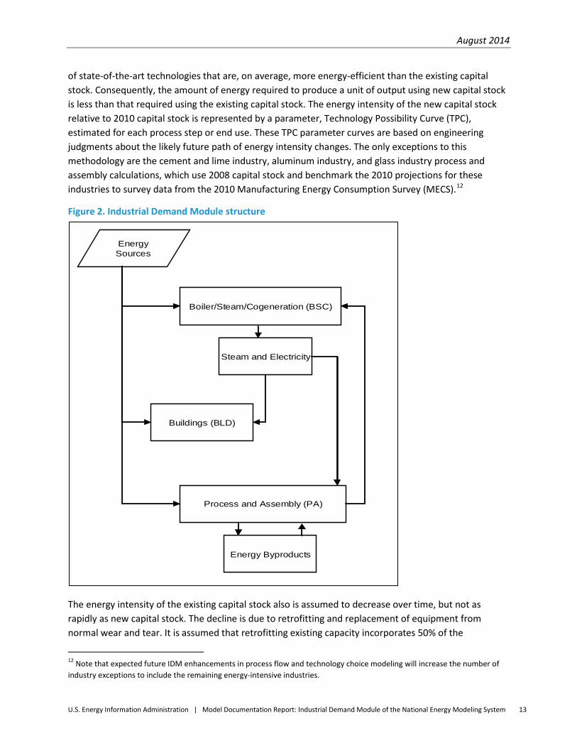
For each industry, the flow of energy among the three model components is represented by the arrows in Figure 2. The BSC component satisfies the steam demand from the PA and BLD components. For the manufacturing industries, the PA component is broken down into the major production processes or end uses. Energy consumption in the IDM is primarily a function of the level of industrial economic activity. Industrial economic activity in NEMS is measured by the dollar value of shipments (in constant 2005 dollars) produced by each industry group. The value of shipments by NAICS classification is provided to the IDM by the NEMS Macroeconomic Activity Module. As the level of industrial economic activity increases, energy consumption typically increases, but at a slower rate than the growth in economic activity.

The amount of energy consumption reported by the Industrial Demand Module is also a function of the vintage of the capital stock that produces the shipments. It is assumed that new capital stock will consist 11 The combination of the cement and lime industries is new in the IDM; hence, there is an incompatibility with any prior AEO that only projects for the cement industry.

August 2014


of state-of-the-art technologies that are, on average, more energy-efficient than the existing capital stock. Consequently, the amount of energy required to produce a unit of output using new capital stock is less than that required using the existing capital stock. The energy intensity of the new capital stock relative to 2010 capital stock is represented by a parameter, Technology Possibility Curve (TPC), estimated for each process step or end use. These TPC parameter curves are based on engineering judgments about the likely future path of energy intensity changes. The only exceptions to this methodology are the cement and lime industry, aluminum industry, and glass industry process and assembly calculations, which use 2008 capital stock and benchmark the 2010 projections for these industries to survey data from the 2010 Manufacturing Energy Consumption Survey (MECS).12

Figure 2. Industrial Demand Module structure

The energy intensity of the existing capital stock also is assumed to decrease over time, but not as rapidly as new capital stock. The decline is due to retrofitting and replacement of equipment from normal wear and tear. It is assumed that retrofitting existing capacity incorporates 50% of the

12 Note that expected future IDM enhancements in process flow and technology choice modeling will increase the number of industry exceptions to include the remaining energy-intensive industries.

Energy Sources

Boiler/Steam/Cogeneration (BSC)

Energy Byproducts

Process and Assembly (PA)

Buildings (BLD)

Steam and Electricity

August 2014


improvement that is achieved by installing new capacity. The net effect is that over time the amount of energy required to produce a unit of output declines. Although total energy consumption in the industrial sector is projected to increase, overall energy intensity is projected to decrease.

Energy consumption in the buildings component is assumed to grow at the same rate as the average growth rate of employment and output in that industry. This formulation has been used to account for the countervailing movements in manufacturing employment and value of shipments. Manufacturing employment falls over the projection, which alone would imply falling building energy use. Because shipments tend to grow fairly rapidly, that implies that conditioned floor space is increasing. Energy consumption in the BSC is assumed to be a function of the steam demand of the other two components.

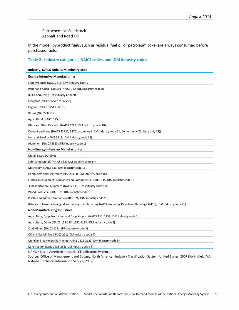
Industry disaggregation Table 2 identifies 6 non-manufacturing and 15 manufacturing industries modeled in the industrial sector along with their NAICS code coverage. These industry groups have been chosen for a variety of reasons. The primary consideration is the distinction between energy-intensive groups and non-energy-intensive industry groups. The energy-intensive industries are modeled in more detail, with aggregate process flows. The industry categories are also chosen to be as consistent as possible with the categories that are available from 2010 MECS. Of the manufacturing industries, seven of the most energy-intensive are modeled in greater detail in the Industrial Demand Module. Energy consumption for Petroleum Refining (NAICS 32411), also an energy-intensive industry, is modeled by the Liquid Fuels Market Module of NEMS.

Energy sources modeled The IDM estimates energy consumption by 21 industries for 14 primary and secondary energy sources, some of which have nonfuel uses. The energy sources modeled in the IDM are:

Sources used in fuel applications:

Electricity Natural Gas Steam Coal Distillate Oil Residual Oil Natural Gas Liquids (NGL) for heat and power; NGL is sometimes reported as Liquefied Petroleum Gas Motor Gasoline Renewables, specifically biomass and hydropower Coking Coal, (including net imports) Petroleum Coke

Sources used in nonfuel applications:

Natural Gas Feedstock NGL Feedstock

August 2014


Petrochemical Feedstock Asphalt and Road Oil

In the model, byproduct fuels, such as residual fuel oil or petroleum coke, are always consumed before purchased fuels.

Table 2. Industry categories, NAICS codes, and IDM industry codes

Industry, NAICS code, IDM industry code Energy-Intensive Manufacturing Food Products (NAICS 311; IDM industry code 7)

Paper and Allied Products (NAICS 322; IDM industry code 8)

Bulk Chemicals (IDM Industry Code 9)

Inorganic (NAICS 32512 to 32518)

Organic (NAICS 32511, 32519)

Resins (NAICS 3252)

Agricultural (NAICS 3253)

Glass and Glass Products (NAICS 3272; IDM industry code 10)

Cement and Lime (NAICS 32731, 32741; combined IDM industry code 11, Cement only 22, Lime only 23))

Iron and Steel (NAICS 3311; IDM industry code 12)

Aluminum (NAICS 3313; IDM industry code 13)

Non-Energy-Intensive Manufacturing

Metal-Based Durables

Fabricated Metals (NAICS 332; IDM industry code 14)

Machinery (NAICS 333; IDM industry code 15)

Computers and Electronics (NAICS 334; IDM industry code 16)

Electrical Equipment, Appliance and Components (NAICS 335; IDM industry code 18)

Transportation Equipment (NAICS 336; IDM industry code 17)

Wood Products (NAICS 321; IDM industry code 19)

Plastic and Rubber Products (NAICS 326; IDM industry code 20)

Balance of Manufacturing (all remaining manufacturing NAICS, excluding Petroleum Refining (32410); IDM industry code 21)

Non-Manufacturing Industries

Agriculture, Crop Production and Crop Support (NAICS 111, 1151; IDM industry code 1)

Agriculture, Other (NAICS 112-113, 1152-1153; IDM industry code 2)

Coal Mining (NAICS 2121; IDM industry code 3)

Oil and Gas Mining (NAICS 211; IDM industry code 4)

Metal and Non-metallic Mining (NAICS 2122-2123; IDM industry code 5)

Construction (NAICS 233-235; IDM industry code 6)

NAICS = North American Industrial Classification System. Source: Office of Management and Budget, North American Industry Classification System, United States, 2007 (Springfield, VA, National Technical Information Service, 2007).

August 2014


Key computations The key computations of the Industrial Demand Module are the Unit Energy Consumption (UEC) estimates made for each NAICS industry group. UEC is defined as the amount of energy required to produce one dollar's worth of shipments or physical output. The distinction between existing and new capital equipment is maintained with a vintage-based accounting procedure. In practice, the fuel use in similar capital equipment is the same across vintages. For example, an electric arc furnace primarily consumes electricity no matter whether it is an old electric arc furnace or a new one.

The modeling approach incorporates technical change in the production process to achieve lower energy intensity. Autonomous technical change can be envisioned as a learning-by-doing process for existing technology. As experience is gained with a technology, the costs of production decline. Autonomous technical change is assumed to be the most important source of energy-related changes in the IDM. Few industrial innovations are adopted solely because of their energy consumption characteristics, but rather for a combination of factors, including process changes to improve product quality, changes made to improve productivity, or changes made in response to the competitive environment. These strategic decisions are not readily amenable to economic or engineering modeling at the current level of disaggregation in the IDM. Instead, the IDM is designed to incorporate overall changes in energy use on a more aggregate and long-term basis using the autonomous technical change parameters.

Buildings component UEC Buildings are estimated to account for a small percentage of allocated heat and power energy in manufacturing industries.13 Detailed projections of manufacturing sector building energy consumption are available upon request from the Industrial Team. Energy consumption in manufacturing buildings is assumed to grow at the average of the growth rates of employment and shipments in that industry. This assumption appears to be reasonable since lighting and heating, ventilation, and air conditioning (HVAC) are designed primarily for workers rather than machines. However, since value of shipments tends to grow, it is likely that conditioned floor space also grows. The IDM uses an average to account for the contrasting trends in employment and shipment growth rates.

Process and assembly component UEC The process and assembly (PA) component is the largest share of direct energy consumption. To derive energy use estimates for the process steps, the production process for each industry was first decomposed into its major steps, and then the engineering and product flow relationships among the steps were specified. Process steps for each industry were analyzed using one of the following two methodologies:

Process flowsheet method. Develop a process flowsheet and estimates of energy use by process step. This was applied to those industries where the process flows could be well defined for a single broad product line by unit process step: paper and allied products, glass and glass products, cement and lime, iron and steel, and aluminum.

13 U.S. Energy Information Administration, 2010 Manufacturing Energy Consumption Survey, (http://www.eia.gov/consumption/manufacturing/), March 2013. Note that byproduct and non-energy use of combustible fuels are excluded from the computation because they are not allocated in the MECS tables.

mailto:[email protected]

http://www.eia.gov/consumption/manufacturing/

August 2014


End-use method. Develop end-use estimates of energy use by generic process unit as a percentage of total energy use in the PA component. This is used where the diversity of end products and unit processes is relatively large: food products, bulk chemicals, metal-based durables, plastic products, wood products, and the balance of manufacturing. A motor stock model, which is described on page 33, calculates the electricity consumption for the machine drive end use for these five industries or industry groups.

In both methodologies, major components of energy consumption are identified by process for various energy sources:

Fossil fuels, which include petroleum products, natural gas, and coal Electricity (valued at 3,412 Btu/kWh) Steam Non-fuel energy sources, such as feedstocks

The following sections present a more detailed discussion of the process steps and unit energy consumption estimates for each of the energy-intensive industries. The data tables showing the estimates are presented in Appendix B and are referenced in the text as appropriate. The process steps are model inputs with the variable name INDSTEPNAME.

Energy-intensive manufacturing industries

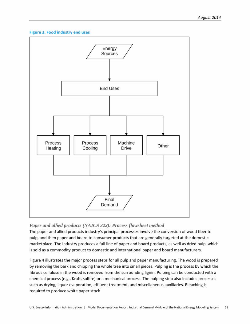
Food products (NAICS 311): End-use method Energy use in the food products industry for the PA component was estimated for each of four major end-use categories:

Process Heating Process Cooling Machine Drive All Other Uses

Figure 3 portrays the PA component's end-use energy flow for the food products industry. A motor stock model, described on page 33, calculates electricity consumption for the machine drive end use. The dominant end use was direct heat, which accounted for 50% of the total PA energy consumption

August 2014


Figure 3. Food industry end uses

Energy Sources

End Uses

Process Heating

Final Demand

Machine Drive Other Process

Cooling

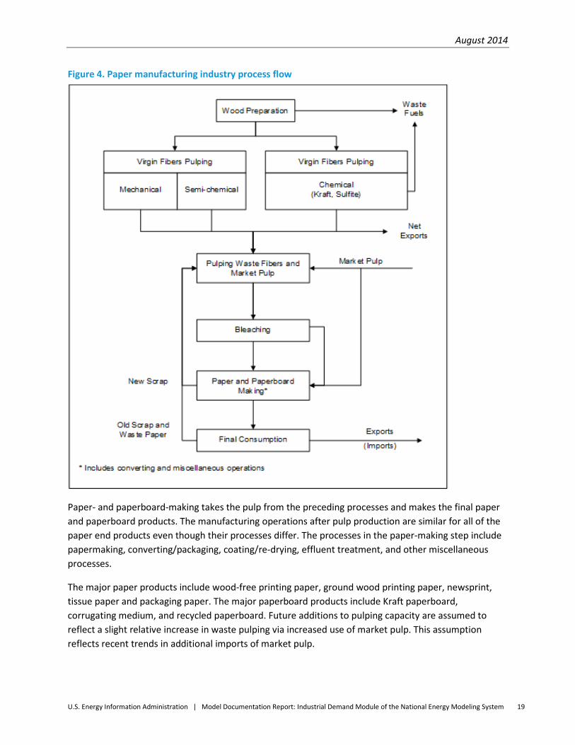
Paper and allied products (NAICS 322): Process flowsheet method The paper and allied products industry's principal processes involve the conversion of wood fiber to pulp, and then paper and board to consumer products that are generally targeted at the domestic marketplace. The industry produces a full line of paper and board products, as well as dried pulp, which is sold as a commodity product to domestic and international paper and board manufacturers.

Figure 4 illustrates the major process steps for all pulp and paper manufacturing. The wood is prepared by removing the bark and chipping the whole tree into small pieces. Pulping is the process by which the fibrous cellulose in the wood is removed from the surrounding lignin. Pulping can be conducted with a chemical process (e.g., Kraft, sulfite) or a mechanical process. The pulping step also includes processes such as drying, liquor evaporation, effluent treatment, and miscellaneous auxiliaries. Bleaching is required to produce white paper stock.

August 2014


Figure 4. Paper manufacturing industry process flow

Paper- and paperboard-making takes the pulp from the preceding processes and makes the final paper and paperboard products. The manufacturing operations after pulp production are similar for all of the paper end products even though their processes differ. The processes in the paper-making step include papermaking, converting/packaging, coating/re-drying, effluent treatment, and other miscellaneous processes.

The major paper products include wood-free printing paper, ground wood printing paper, newsprint, tissue paper and packaging paper. The major paperboard products include Kraft paperboard, corrugating medium, and recycled paperboard. Future additions to pulping capacity are assumed to reflect a slight relative increase in waste pulping via increased use of market pulp. This assumption reflects recent trends in additional imports of market pulp.

August 2014


Bulk chemical industry (parts of NAICS 325): End-use method The bulk chemical sector is very complex. Industrial inorganic and organic chemicals are basic chemicals, while plastics, agricultural chemicals, synthetic rubber, pharmaceuticals, and other chemicals are either intermediate chemicals or final products. This industry is a major energy feedstock user and a major producer of combined heat and power.

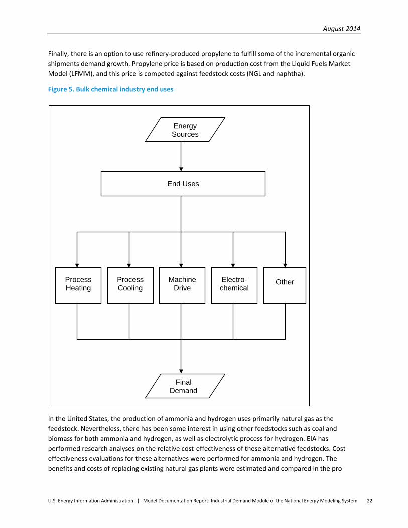
The bulk chemical industry’s energy consumption patterns are equally complex, with demands for heat, steam, electricity, and energy feedstocks driven by the demand for production of numerous chemical products, as well as the processes and technologies involved in making these products. Because of this complexity, only ethanol and hydrogen production are singled out for the tracking of specific energy consumption as these chemicals are incorporated directly into the supply modules of NEMS. The rest of the chemicals are aggregated into the four categories as defined by NAICS codes, shown below in Table 3. There are 15 organic, 5 inorganic, 5 resins, and 2 agricultural chemicals, plus 4 aggregate (“other”) groups. Modeling of energy consumption within these groups is accomplished by the Technology Possibility Curve (TPC) method used for most other industries as described in Figure 5 and under the “Key computations” section on page 11. A limited feedstock selection algorithm is included as well (see below).

The delineation of feedstock demand applies only to the PA component of the bulk chemical energy consumption projections. The PA component also estimates energy consumption for direct process heating, cooling, machine drive, motors, and other uses. The BSC and BLD components remain the same for this industry as in other models. Thus, steam demand projections are passed from the PA component to the BSC component. The BSC component then calculates fuel consumption to generate the steam. Also, as in the other modules, the BLD component projects energy consumption for this industry’s use of its facilities for space heating, space cooling, and lighting.

August 2014


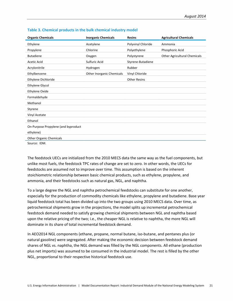
Table 3. Chemical products in the bulk chemical industry model

Organic Chemicals Inorganic Chemicals Resins Agricultural Chemicals Ethylene Acetylene Polyvinyl Chloride Ammonia

Propylene Chlorine Polyethylene Phosphoric Acid

Butadiene Oxygen Polystyrene Other Agricultural Chemicals

Acetic Acid Sulfuric Acid Styrene-Butadiene

Acrylonitrile Hydrogen Rubber

Ethylbenzene Other Inorganic Chemicals Vinyl Chloride

Ethylene Dichloride Other Resins

Ethylene Glycol

Ethylene Oxide

Formaldehyde

Methanol

Styrene

Vinyl Acetate

Ethanol

On-Purpose Propylene (and byproduct

ethylene)

Other Organic Chemicals Source: IDM.

The feedstock UECs are initialized from the 2010 MECS data the same way as the fuel components, but unlike most fuels, the feedstock TPC rates of change are set to zero. In other words, the UECs for feedstocks are assumed not to improve over time. This assumption is based on the inherent stoichiometric relationship between basic chemical products, such as ethylene, propylene, and ammonia, and their feedstocks such as natural gas, NGL, and naphtha.

To a large degree the NGL and naphtha petrochemical feedstocks can substitute for one another, especially for the production of commodity chemicals like ethylene, propylene and butadiene. Base year liquid feedstock total has been divided up into the two groups using 2010 MECS data. Over time, as petrochemical shipments grow in the projections, the model splits up incremental petrochemical feedstock demand needed to satisfy growing chemical shipments between NGL and naphtha based upon the relative pricing of the two; i.e., the cheaper NGL is relative to naphtha, the more NGL will dominate in its share of total incremental feedstock demand.

In AEO2014 NGL components (ethane, propane, normal butane, iso-butane, and pentanes plus (or natural gasoline) were segregated. After making the economic decision between feedstock demand shares of NGL vs. naphtha, the NGL demand was filled by the NGL components. All ethane (production plus net imports) was assumed to be consumed in the industrial model. The rest is filled by the other NGL, proportional to their respective historical feedstock use.

August 2014


Finally, there is an option to use refinery-produced propylene to fulfill some of the incremental organic shipments demand growth. Propylene price is based on production cost from the Liquid Fuels Market Model (LFMM), and this price is competed against feedstock costs (NGL and naphtha).

Figure 5. Bulk chemical industry end uses

End Uses

Energy Sources

Final Demand

Process Heating

Process Cooling

Machine Drive

Electro-chemical

Other

In the United States, the production of ammonia and hydrogen uses primarily natural gas as the feedstock. Nevertheless, there has been some interest in using other feedstocks such as coal and biomass for both ammonia and hydrogen, as well as electrolytic process for hydrogen. EIA has performed research analyses on the relative cost-effectiveness of these alternative feedstocks. Cost-effectiveness evaluations for these alternatives were performed for ammonia and hydrogen. The benefits and costs of replacing existing natural gas plants were estimated and compared in the pro

August 2014


forma analysis. The competition between natural gas and the alternatives for a new plant was also analyzed. The costs of using the alternatives were found to be significantly prohibitive, and continue to be in light of continued relatively inexpensive natural gas due to increasing domestic supply. This issue continues to be studied by EIA and will be updated in future projections as appropriate.

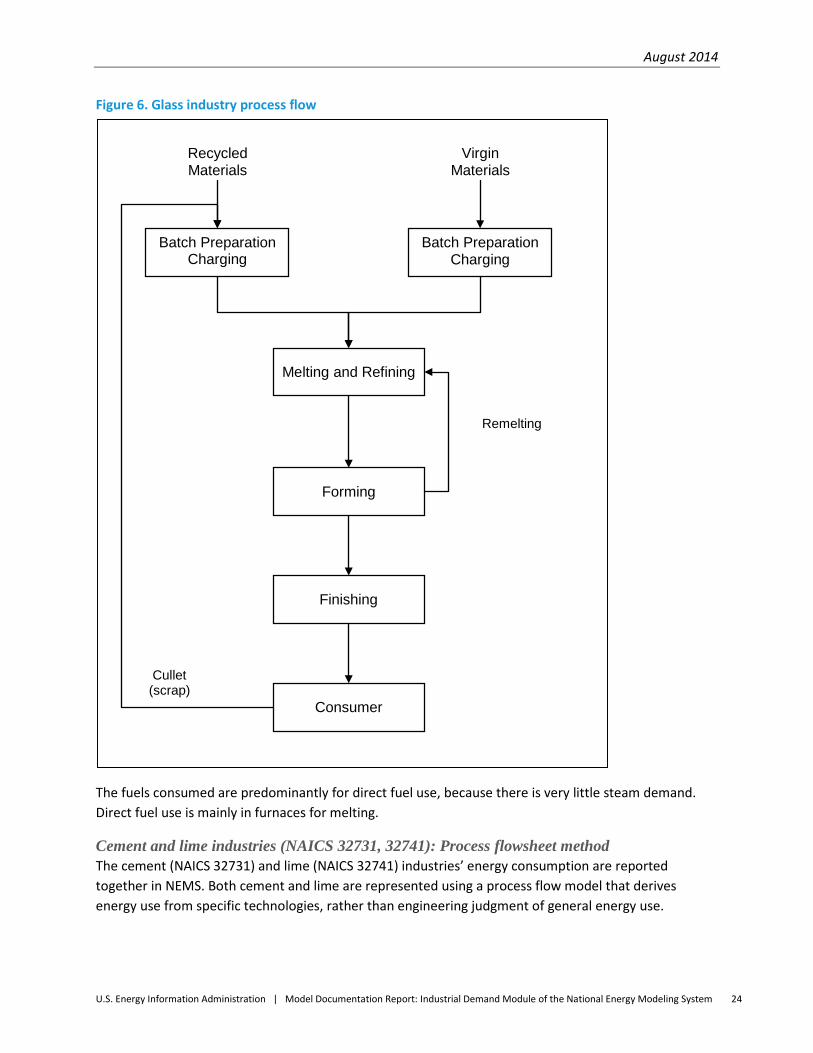
Glass and glass products industry (NAICS 3272): Process flowsheet method An energy use profile has been developed for the whole glass and glass products industry, NAICS 3272. This industry definition includes glass products made from purchased glass. The glass-making process contains four process steps: batch preparation, melting/refining, forming and finishing. Figure 6 provides an overview of the process steps involved in the glass and glass products industry. While cullet (scrap) and virgin materials are shown separately to account for the different energy requirements for cullet and virgin material melting, glass makers generally mix cullet with the virgin material.

August 2014


Figure 6. Glass industry process flow

Batch Preparation Charging

Batch Preparation Charging

Virgin Materials

Recycled Materials

Melting and Refining

Forming

Finishing

Consumer

Remelting

Cullet (scrap)

The fuels consumed are predominantly for direct fuel use, because there is very little steam demand. Direct fuel use is mainly in furnaces for melting.

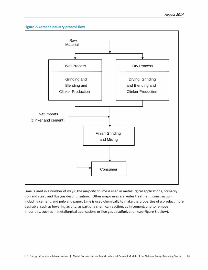
Cement and lime industries (NAICS 32731, 32741): Process flowsheet method The cement (NAICS 32731) and lime (NAICS 32741) industries’ energy consumption are reported together in NEMS. Both cement and lime are represented using a process flow model that derives energy use from specific technologies, rather than engineering judgment of general energy use.

August 2014


The cement industry uses raw materials from non-manufacturing quarrying and mining industries. These materials are sent through crushing and grinding mills and converted to clinker in the clinker-producing step. This clinker is then further ground to produce cement. The industry produces cement by two major processes: the wet process and the dry process. The dry process is less energy-intensive than the wet process, and thus the dry process has steadily gained favor in cement production. As a result, it is assumed in the model that all new plants will be based on the dry process. Figure 7 provides an overview of the process steps involved in the cement industry.

Since cement is the primary binding ingredient in concrete mixtures, it is used in virtually all types of construction. As a result, the U.S. demand for cement is highly sensitive to the level of construction activity, which is projected for NEMS using the Macroeconomic Activity Module and transferred to the IDM as an input.

August 2014


Figure 7. Cement industry process flow

Wet Process

Grinding and Blending and

Clinker Production

Dry Process

Drying, Grinding and Blending and Clinker Production

Finish Grinding and Mixing

Raw Material

Consumer

Net Imports (clinker and cement)

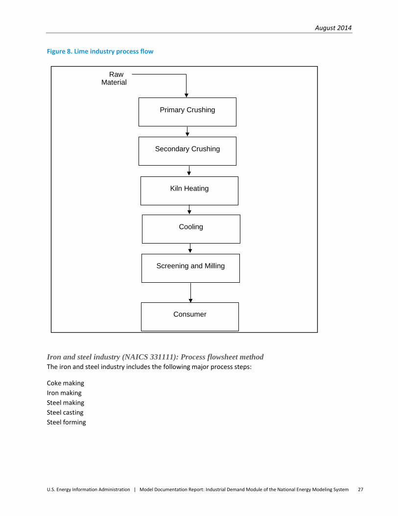
Lime is used in a number of ways. The majority of lime is used in metallurgical applications, primarily iron and steel, and flue gas desulfurization. Other major uses are water treatment, construction, including cement, and pulp and paper. Lime is used chemically to make the properties of a product more desirable, such as lowering acidity; as part of a chemical reaction, as in cement; and to remove impurities, such as in metallurgical applications or flue gas desulfurization (see Figure 8 below).

August 2014


Figure 8. Lime industry process flow

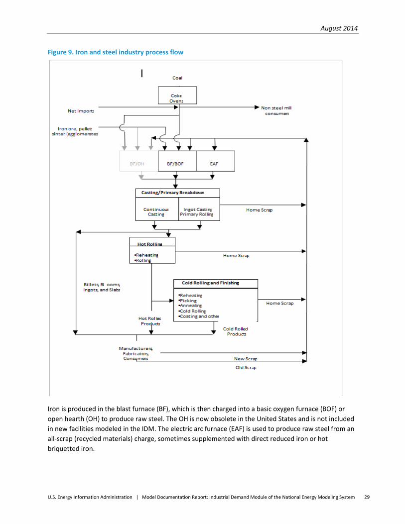
Iron and steel industry (NAICS 331111): Process flowsheet method The iron and steel industry includes the following major process steps:

Coke making Iron making Steel making Steel casting Steel forming

Raw Material

Secondary Crushing

Primary Crushing

Kiln Heating

Screening and Milling

Consumer

Cooling

August 2014


Steel manufacturing plants can be classified as integrated or non-integrated. The classification is dependent upon the number of the major process steps that are performed in the facility. Integrated plants perform all the process steps, whereas non-integrated plants, in general, perform only the last three steps.

For the Industrial Demand Module, a process flow was developed to separate the process into five steps around which unit energy consumption values were estimated.

Figure 9 shows the process flow diagram used for the analysis. An agglomeration step is excluded from the IDM iron and steel submodule because it is considered part of mining. Iron ore and coal are the basic raw materials that are used to produce iron.

August 2014


Figure 9. Iron and steel industry process flow

Iron is produced in the blast furnace (BF), which is then charged into a basic oxygen furnace (BOF) or open hearth (OH) to produce raw steel. The OH is now obsolete in the United States and is not included in new facilities modeled in the IDM. The electric arc furnace (EAF) is used to produce raw steel from an all-scrap (recycled materials) charge, sometimes supplemented with direct reduced iron or hot briquetted iron.

August 2014


The largest category for energy use is coal, followed by liquid and gas fuels. Coke ovens and blast furnaces also produce a significant amount of byproduct fuels, which are used throughout the steel plant.

The raw steel is cast into blooms, billets or slabs using continuous casting, or more rarely, ingots. Some ingot or cast steel is sold directly (e.g., forging-grade billets). The majority is further processed (‘hot rolled’) into various mill products. Some of these are sold as hot rolled mill products, while others are further cold rolled to impart surface finish or other desirable properties.

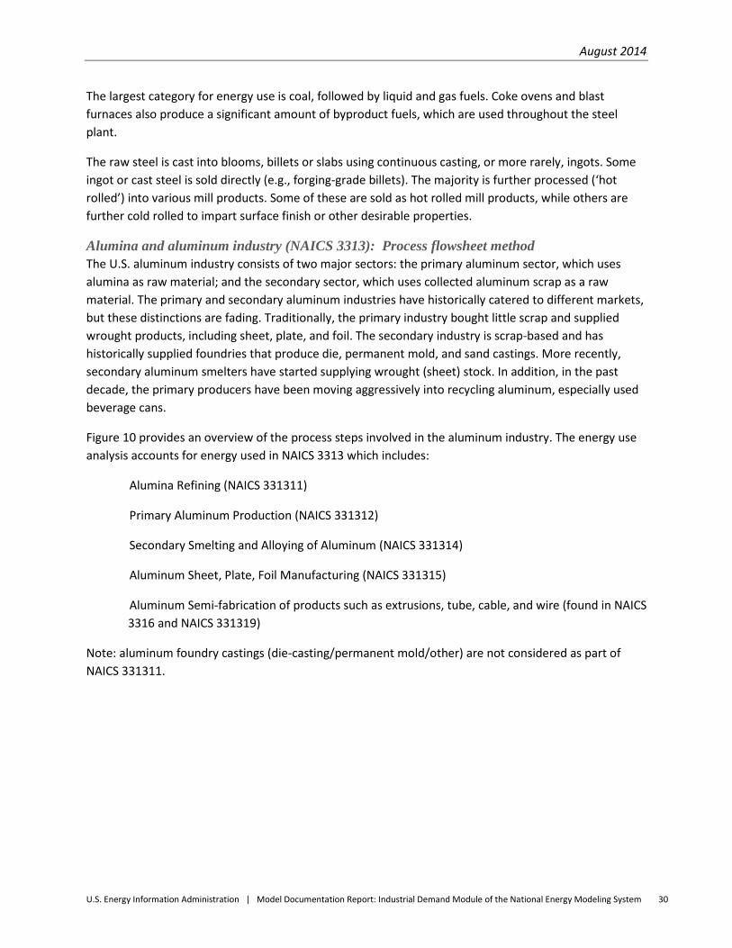
Alumina and aluminum industry (NAICS 3313): Process flowsheet method The U.S. aluminum industry consists of two major sectors: the primary aluminum sector, which uses alumina as raw material; and the secondary sector, which uses collected aluminum scrap as a raw material. The primary and secondary aluminum industries have historically catered to different markets, but these distinctions are fading. Traditionally, the primary industry bought little scrap and supplied wrought products, including sheet, plate, and foil. The secondary industry is scrap-based and has historically supplied foundries that produce die, permanent mold, and sand castings. More recently, secondary aluminum smelters have started supplying wrought (sheet) stock. In addition, in the past decade, the primary producers have been moving aggressively into recycling aluminum, especially used beverage cans.

Figure 10 provides an overview of the process steps involved in the aluminum industry. The energy use analysis accounts for energy used in NAICS 3313 which includes:

Alumina Refining (NAICS 331311)

Primary Aluminum Production (NAICS 331312)

Secondary Smelting and Alloying of Aluminum (NAICS 331314)

Aluminum Sheet, Plate, Foil Manufacturing (NAICS 331315)

Aluminum Semi-fabrication of products such as extrusions, tube, cable, and wire (found in NAICS 3316 and NAICS 331319)

Note: aluminum foundry castings (die-casting/permanent mold/other) are not considered as part of NAICS 331311.

August 2014


Figure 10. Aluminum industry process flow

Alumina Production

Primary Aluminum Smelters

Semi - Fabrication of other Al products

(e.g., extrusions, bars, wires)

Semi - Fabricators Sheet, plate, foil

Scrap Based (Secondary) Aluminum Smelters

Imported Bauxite

Exports (Imports)

of Scrap

Imports (ingot, slab)

New Scrap

End - Product Fabricators

New Scrap

Final Consumption Old Scrap

(Imports) Exports

Imports (alumina)

Ingots, Hot Metal to Aluminum Foundries*

Non-energy-intensive manufacturing industries

Metal-based durables industry group (NAICS 332-336): End-use method This industry group consists of industries that manufacture: fabricated metals; machinery; computer and electronic products; transportation equipment; and electrical equipment, appliances, and components. Typical processes found in this group include re-melting operations followed by casting or molding, shaping, heat-treating processes, coating, and joining and assembly. Given this diversity of processes, the industry group’s energy is represented using the end-use method based on the 2010

August 2014


MECS.14 End-use processes for metal-based durables are the same as in bulk chemicals, as shown in Figure 5. A motor stock model, described on page 33, calculates electricity consumption for the machine drive end use.

Other non-energy-intensive manufacturing industries: End-use method This is a group of miscellaneous industries consisting of wood products, plastic products, and the balance of manufacturing category that includes, among others, tobacco, printing, furniture, and textiles. Data limitations and the lack of a dominant energy user limit disaggregation of these industries. Wood products manufacturing is of interest because the industry derives a majority of its energy from biomass in the form of wood waste and residue. The plastics manufacturing industry produces goods by processing goods from plastic materials but does not produce the plastic. End use processes for metal-based durables are the same as in food products, which are shown in Figure 3.

A motor stock model, described on page 33, calculates electricity consumption for the machine drive end use for balance of manufacturing.

Non-manufacturing industries The non-manufacturing industries do not have MECS as the predominant source for energy consumption data as the manufacturing industries do. Instead, UECs for the agriculture, mining, and construction industries are derived from various sources collected by a number of federal agencies, notably U.S. Department of Agriculture (USDA) and the U.S. Census Bureau, part of the U.S. Department of Commerce. Furthermore, unlike the majority of manufacturing industries, the TPCs for non-manufacturing are not fixed; they change over time. This dynamic process depends on output from other NEMS modules such as the Commercial Demand Module (CDM) and the Transportation Demand Module (TDM) , which are used in the agriculture, construction, and mining models. For mine productivity, oil and gas wells use the Oil and Gas Supply Module (OGSM) and coal mines use input from the Coal Market Module (CMM).

Energy consumption data for the two agriculture sectors (crops and other agriculture) are largely based on information contained in the Census of Agriculture conducted by the U.S. Department of Agriculture,15 and a special tabulation from the USDA-NASS.16 Expenditures for four energy sources were collected for crop farms and livestock farms. These data were converted from dollar expenditures to energy quantities using prices from the Department of Agriculture and EIA.

For AEO2014, non-manufacturing data was revised using EIA and Census Bureau sources to provide more realistic projections of diesel and gasoline for off-road vehicle use, provide more accurate projections of electricity consumption, and allocate natural gas and hydrocarbon gas liquids (HGL) use.

14 U.S. Energy Information Administration (EIA), 2010 Manufacturing Energy Consumption Survey, http://www.eia.gov/consumption/manufacturing/index.cfm, March 2013. 15 U.S. Department of Agriculture, National Agricultural Statistical Service, 2007 Census of Agriculture, February 2009 http://www.agcensus.usda.gov/Publications/2007/index.asp . 16 Jim Duffield, USDA-NASS, 2007 Census of Agriculture Special Tabulation, April 2010, http://www.nass.usda.gov/Data_and_Statistics/Special_Tabulations/index.asp .

http://www.eia.gov/reports/index.cfm?t=Model%20Documentation




http://www.eia.gov/consumption/manufacturing/index.cfm

http://www.agcensus.usda.gov/Publications/2007/index.asp

http://www.nass.usda.gov/Data_and_Statistics/Special_Tabulations/index.asp

August 2014


Sources used are EIA’s Fuel Oil and Kerosene Sales (FOKS)17 for distillate consumption, Agricultural Resource Management Survey (ARMS) 18 and the U.S. Census Bureau’s Census of Mining19 and Census of Construction. 20 Also, the use of hydrocarbon gas liquids (HGL) is now accounted for in the agriculture and especially the construction industries. Non-manufacturing consumption is no longer dictated solely by the SEDS – MECS difference as it has been in previous years. The mining industry is divided into three sectors in the Industrial Demand Module – coal mining, oil and gas extraction, and other mining. The quantities of seven energy types consumed by 29 mining sectors were collected as part of the 2007 Economic Census of Mining by the U.S. Census Bureau. 21 The data for the 29 sectors were aggregated into the three sectors included in the Industrial Demand Module and the physical quantities were converted to Btu for use in NEMS.

Only one construction sector is included in the Industrial Demand Module. Detailed statistics for the 31 construction subsectors included in the 2007 Economic Census were aggregated. Expenditure amounts for five energy sources were collected by the U.S. Census Bureau.21 These expenditures were converted from dollars to energy quantities using EIA prices.

These sources are considered to be the most complete and consistent data available for each of the three non-manufacturing sectors. These data, supplemented by available EIA data, are used to derive total energy consumption for the non-manufacturing industrial sectors. The additional EIA data are from the State Energy Data System 2011. 22 The source data relate to total energy consumption and provide no information on the processes or end uses for which the energy is consumed. Therefore, the UECs for the mining and construction industries relate energy consumption for each fuel type to value of shipments. For the two agricultural industries in the IDM, a submodule was implemented and is described below.

Agricultural submodule U.S. agriculture consists of three major sub-sectors: crop production, which is dependent primarily on regional environments and crops demanded; animal production, which is largely dependent on food demands and feed accessibility; and all remaining agricultural activities, primarily forestry and logging. The energy use analysis accounts for energy used in the following categories, with the second and third category combined for modeling purposes:

Crop Production and Support Activities (NAICS 111 & 1151)

17 U.S. Energy Information Administration, Fuel Oil and Kerosene Survey 2011 (FOKS),(Washington, DC, January 2013) www.eia.gov/petroleum/fueloilkerosene/archive/2012/foks_2012.cfm . 18 Agriculture Research Management Survey (ARMS), United States Dept. of Agriculture, Economic Research Service 2011, (Washington DC, November 27, 2012) http://www.ers.usda.gov/data-products/arms-farm-financial-and-crop-production-practices.aspx#.UxcWZ_ldWCm . 19 U.S. Census Bureau, 2007 Economic Census, Mining Industry Series, (Washington DC 2009) http://factfinder2.census.gov/faces/tableservices/jsf/pages/productview.xhtml?pid=ECN_2007_US_21SG12&prodType=table . 20 U.S. Census Bureau 2007 Economic Census, Construction Summary Series, (Washington DC 2009), http://factfinder2.census.gov/faces/tableservices/jsf/pages/productview.xhtml?pid=ECN_2007_US_23SG01&prodType=table. 21 U.S. Department of Commerce, Census Bureau, Economic Census 2007: Mining and Construction Industry Series, 2009, http://www.census.gov/econ/census07/. 22 Energy Information Administration, State Energy Data System 2011 (Washington, DC, June 2011).

http://www.eia.gov/petroleum/fueloilkerosene/archive/2012/foks_2012.cfm

http://www.ers.usda.gov/data-products/arms-farm-financial-and-crop-production-practices.aspx%23.UxcWZ_ldWCm

http://www.ers.usda.gov/data-products/arms-farm-financial-and-crop-production-practices.aspx%23.UxcWZ_ldWCm

http://factfinder2.census.gov/faces/tableservices/jsf/pages/productview.xhtml?pid=ECN_2007_US_21SG12&prodType=table

http://factfinder2.census.gov/faces/tableservices/jsf/pages/productview.xhtml?pid=ECN_2007_US_23SG01&prodType=table.

http://www.census.gov/econ/census02/guide/INDRPT21.HTM

http://www.census.gov/econ/census02/guide/INDRPT21.HTM

August 2014


Animal Production and Support Activities (NAICS 112 & 1152)

Forestry and Logging and Support Activities (NAICS 113 & 1153)

Consumption in these industries is tied to specialized equipment, which often determines the fuel requirement with little flexibility. Within each of these sub-industries the key energy-using equipment can be broken into three major categories: off-road vehicles, buildings, and other equipment, which is primarily irrigation equipment for crop production.23 In the IDM, building energy consumption is driven by building characteristics retrieved from the NEMS Commercial Demand Module, and vehicle energy consumption is driven by vehicle efficiencies, by type of fuel, retrieved from the NEMS Transportation Demand Module.

Mining submodule The mining sector comprises three subsectors: coal mining, metal and nonmetal mining, and oil and gas extraction. Energy use is based on what equipment is used at the mine and onsite vehicles used. All mines use extraction equipment and lighting, but only coal and metal and nonmetal mines use grinding and ventilation. Characteristic of the non-manufacturing sector, TPCs are influenced by efficiency changes in buildings and transportation equipment.

Coal mining production is obtained from the NEMS Coal Market Module (CMM). Currently, it is assumed that approximately 70% of the coal is mined at the surface and the rest is mined underground. As these shares evolve, however, so does the energy consumed because surface mines use less energy overall than underground mining. Moreover, the energy consumed for coal mining depends on coal mine productivity, which is also obtained from the CMM. Distillate fuel and electricity are the predominant fuels used in coal mining. Electricity used for coal grinding is calculated using the raw grinding process step from the cement submodule described beginning on page 92. In metal and non-metal mining, energy use is similar to coal mining. Output used for metal and non-metal mining is derived from the Macroeconomic Analysis Module’s variable for “other” mining which also provides the shares of each.

For oil and natural gas extraction, production is derived from the OGSM. Energy use depends upon the fuel extracted as well as whether the well is conventional or unconventional, e.g., extraction from tight and shale formations, percentage of dry wells, and well depth.

Construction submodule Construction uses distillate, gasoline, asphalt and road oil, as well as electricity and natural gas. Asphalt and road oil are tied to state and local government real investment in highways and streets, and this investment is derived from the MAM. TPCs for diesel and gasoline fuels are directly tied to the Transportation Demand Module’s heavy- and medium-duty vehicle efficiency projections. For non-vehicular construction equipment, TPCs are a weighted average of vehicular TPCs and highway investment.

23 Edward Eugeni, SRA International “Report on the Analysis and Modeling Approach to Characterize and Estimate Fuel Use by End-Use Applications in the Agriculture and Construction Industries,” (Washington, DC: March 2011)

August 2014


Technology possibility curves, unit energy consumption, and relative energy intensities Technology possibility curves are used to derive future improvements in unit energy consumption. Future energy improvements were estimated for old (retrofit) and new processes/facilities. The energy improvements for grouped old facilities consist of gradual improvements due to energy conservation measures, retrofit of selected technologies, and the closure of older facilities, leaving the more-efficient plants in operation. The energy savings for old processes/facilities were estimated using engineering judgment regarding how much energy savings could be reasonably achieved in each industry. The estimated annual energy savings for each energy conservation measure are up to 0.5% per year.

UEC values for the state-of-the-art (SOA) and advanced technologies are also estimated. SOA technologies are the latest proven technologies that are available at the time a commitment is made to build a new plant. These values are then compared to the 2010 UEC values to develop an index of relative energy intensity (REI). Relative energy intensity is defined as the ratio of energy use in a new or advanced process compared to 2010 average energy use.

The efficiency improvement for new facilities assumes that the installation includes the SOA technologies available for that industry. A second, and at times more important, set of substantial improvements can occur when advanced technologies become available for a specific process. Often one sees a number of technologies being developed and it is difficult to ascertain which specific technologies will be successful. Some judgment is necessary as to the energy-saving potential and the likelihood for such savings to be realistically achieved. All energy improvements in the Industrial Demand Module are based on 2010 energy usage.

Additionally, even SOA technologies and advanced technologies can sometimes be expected to improve after development as the process is improved, optimal residence times and temperatures are found, and better energy recovery techniques are installed. Depending on the process, these are factored into the projections as slow improvements ranging from zero to a maximum of just under 1% per year.

Old facilities are assumed to be able to economically justify some retrofits and, for other reasons listed above, show slow improvements over time in their unit energy consumption. It is assumed that by 2040, old equipment (2010 stock) still operating can achieve up to 50% of the energy savings of SOA technology due to retrofits and other reasons listed above. Thus, if SOA technology has an REI of 0.80, old equipment operating in the year 2040 will have an REI of 0.90. As a convenience for modeling purposes, the rate of change between the initial and final points is defined as the technology possibility curve (TPC) and used to interpolate for the intervening points.

Advanced technologies are ones that are still under development and will be available at some time in the future. It is uncertain which specific technologies will be implemented, but it can be assumed with reasonable certainty that at least one of these technologies or a similar technology will be successful. It is also recognized that in some instances thermodynamic limits are being approached, which will prevent further significant improvements in energy savings.

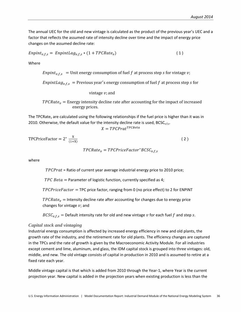
August 2014


The annual UEC for the old and new vintage is calculated as the product of the previous year’s UEC and a factor that reflects the assumed rate of intensity decline over time and the impact of energy price changes on the assumed decline rate:

𝐸𝑛𝑝𝑖𝑛𝑡𝑣,𝑓,𝑠 = 𝐸𝑛𝑝𝑖𝑛𝑡𝐿𝑎𝑔𝑣,𝑓,𝑠 ∗ (1 + 𝑇𝑃𝐶𝑅𝑎𝑡𝑒𝑣) ( 1 )

Where

𝐸𝑛𝑝𝑖𝑛𝑡𝑣,𝑓,𝑠 = Unit energy consumption of fuel 𝑓 at process step 𝑠 for vintage 𝑣;

𝐸𝑛𝑝𝑖𝑛𝑡𝐿𝑎𝑔𝑣,𝑓,𝑠 = Previous year′s energy consumption of fuel 𝑓 at process step 𝑠 for

vintage 𝑣; and

𝑇𝑃𝐶𝑅𝑎𝑡𝑒𝑣 = Energy intensity decline rate after accounting for the impact of increased energy prices.

The TPCRatev are calculated using the following relationships if the fuel price is higher than it was in 2010. Otherwise, the default value for the intensity decline rate is used, BCSCv,f,s.

𝑋 = 𝑇𝑃𝐶𝑃𝑟𝑎𝑡𝑇𝑃𝐶𝐵𝑒𝑡𝑎

TPCPriceFactor = 2∗ X(1+X) ( 2 )

𝑇𝑃𝐶𝑅𝑎𝑡𝑒𝑣 = 𝑇𝑃𝐶𝑃𝑟𝑖𝑐𝑒𝐹𝑎𝑐𝑡𝑜𝑟∗𝐵𝐶𝑆𝐶𝑣,𝑓,𝑠

where

𝑇𝑃𝐶𝑃𝑟𝑎𝑡 = Ratio of current year average industrial energy price to 2010 price;

𝑇𝑃𝐶 𝐵𝑒𝑡𝑎 = Parameter of logistic function, currently specified as 4;

𝑇𝑃𝐶𝑃𝑟𝑖𝑐𝑒𝐹𝑎𝑐𝑡𝑜𝑟 = TPC price factor, ranging from 0 (no price effect) to 2 for ENPINT

𝑇𝑃𝐶𝑅𝑎𝑡𝑒𝑣 = Intensity decline rate after accounting for changes due to energy price changes for vintage 𝑣; and

𝐵𝐶𝑆𝐶𝑣,𝑓,𝑠 = Default intensity rate for old and new vintage 𝑣 for each fuel 𝑓 and step 𝑠.

Capital stock and vintaging Industrial energy consumption is affected by increased energy efficiency in new and old plants, the growth rate of the industry, and the retirement rate for old plants. The efficiency changes are captured in the TPCs and the rate of growth is given by the Macroeconomic Activity Module. For all industries except cement and lime, aluminum, and glass, the IDM capital stock is grouped into three vintages: old, middle, and new. The old vintage consists of capital in production in 2010 and is assumed to retire at a fixed rate each year.

Middle vintage capital is that which is added from 2010 through the Year-1, where Year is the current projection year. New capital is added in the projection years when existing production is less than the

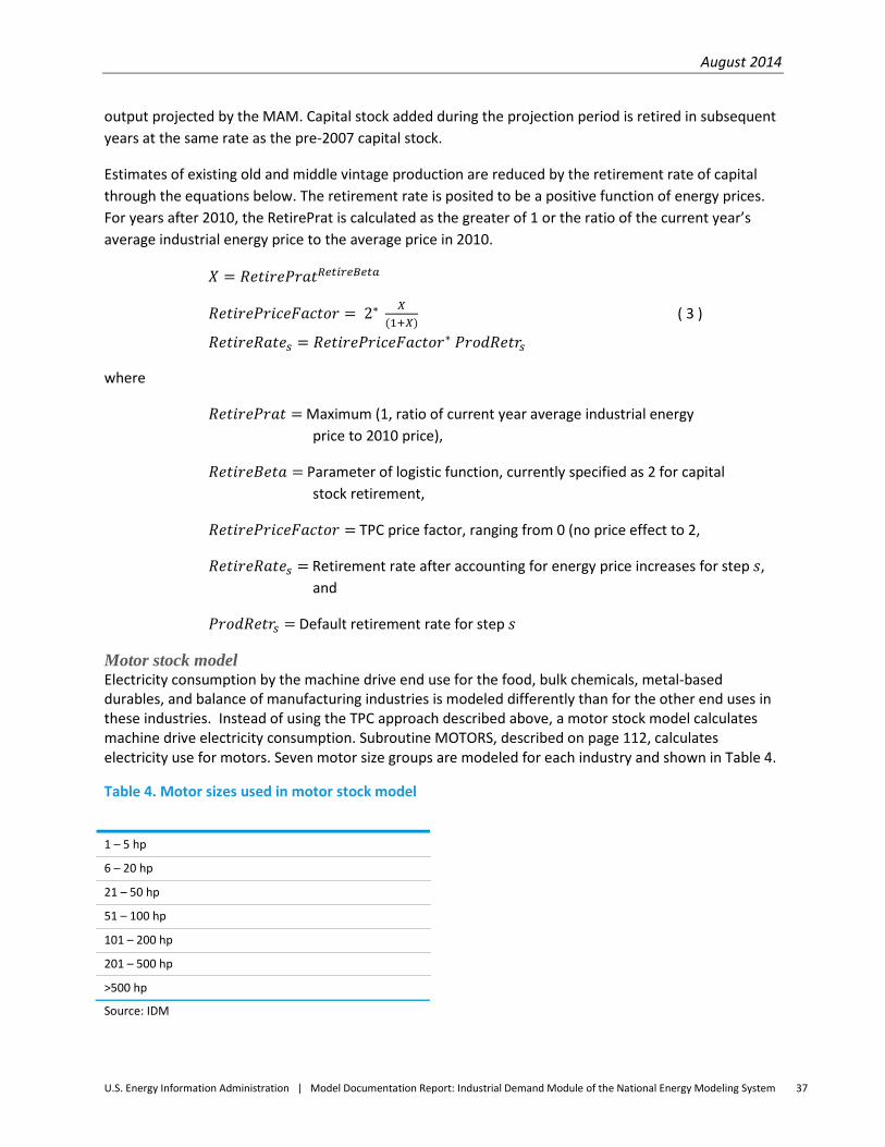
August 2014


output projected by the MAM. Capital stock added during the projection period is retired in subsequent years at the same rate as the pre-2007 capital stock.

Estimates of existing old and middle vintage production are reduced by the retirement rate of capital through the equations below. The retirement rate is posited to be a positive function of energy prices. For years after 2010, the RetirePrat is calculated as the greater of 1 or the ratio of the current year’s average industrial energy price to the average price in 2010.

𝑋 = 𝑅𝑒𝑡𝑖𝑟𝑒𝑃𝑟𝑎𝑡𝑅𝑒𝑡𝑖𝑟𝑒𝐵𝑒𝑡𝑎

𝑅𝑒𝑡𝑖𝑟𝑒𝑃𝑟𝑖𝑐𝑒𝐹𝑎𝑐𝑡𝑜𝑟 = 2∗ 𝑋(1+𝑋)

( 3 )

𝑅𝑒𝑡𝑖𝑟𝑒𝑅𝑎𝑡𝑒𝑠 = 𝑅𝑒𝑡𝑖𝑟𝑒𝑃𝑟𝑖𝑐𝑒𝐹𝑎𝑐𝑡𝑜𝑟∗ 𝑃𝑟𝑜𝑑𝑅𝑒𝑡𝑟𝑠

where

𝑅𝑒𝑡𝑖𝑟𝑒𝑃𝑟𝑎𝑡 = Maximum (1, ratio of current year average industrial energy price to 2010 price),

𝑅𝑒𝑡𝑖𝑟𝑒𝐵𝑒𝑡𝑎 = Parameter of logistic function, currently specified as 2 for capital stock retirement,

𝑅𝑒𝑡𝑖𝑟𝑒𝑃𝑟𝑖𝑐𝑒𝐹𝑎𝑐𝑡𝑜𝑟 = TPC price factor, ranging from 0 (no price effect to 2,

𝑅𝑒𝑡𝑖𝑟𝑒𝑅𝑎𝑡𝑒𝑠 = Retirement rate after accounting for energy price increases for step 𝑠, and

𝑃𝑟𝑜𝑑𝑅𝑒𝑡𝑟𝑠 = Default retirement rate for step 𝑠

Motor stock model Electricity consumption by the machine drive end use for the food, bulk chemicals, metal-based durables, and balance of manufacturing industries is modeled differently than for the other end uses in these industries. Instead of using the TPC approach described above, a motor stock model calculates machine drive electricity consumption. Subroutine MOTORS, described on page 112, calculates electricity use for motors. Seven motor size groups are modeled for each industry and shown in Table 4.

Table 4. Motor sizes used in motor stock model

1 – 5 hp 6 – 20 hp 21 – 50 hp 51 – 100 hp 101 – 200 hp 201 – 500 hp >500 hp Source: IDM

August 2014


The data for the basic motor stock model were derived from United States Industrial Electric Motor Systems Market Opportunities Assessment, 24 a report produced for the U.S. Department of Energy’s Office of Industrial Technologies. Section 313 of The Energy Independence and Security Act of 2007 (EISA2007) increased the minimum efficiency of motors to reflect the National Electrical Manufacturers Association’s ‘Premium Efficiency’ requirements, effective no later than 2011. These revised standards simplify the model code since only premium-efficiency motors can be purchased.

The motor stock model can be broken down into several steps. The steps are outlined as follows:

• Evaluate rewind/replace decision for failed motors.

o For each failed motor, evaluate whether the motor is repaired or replaced. The cost and performance characteristics for the motor options are from the MotorMaster+ version 4.0 software. o Determine the cost differential for replacing the motor. This is the difference between the cost of the new motor meeting minimum efficiency standards and the cost of repairing the motor. o Determine the annual electricity expenditure savings from replacing the motor. This calculation requires the rated motor horsepower, the average motor part-load, the conversion factor from horsepower to kilowatts, the annual operating hours for the motor, the industrial electricity price, the efficiency rating for minimum efficiency motor, and the efficiency rating for a repaired motor. For purposes of the analysis, the electricity price is assumed to remain constant at the level in the year the choice is made. o Determine the payback period needed to recover the cost differential for replacing the motor. The payback is determined by dividing the new motor cost differential by the annual electricity expenditure savings. o Assess the market penetration for replacement motors based on the payback period and the payback acceptance curve.

• Estimate annual change in industry motor stock and industry motor efficiency as a result of rewinds and replacements.

o Given the payback for each motor size group in each industry, estimate the fraction of replacement motors purchased. This analysis begins with an assumed distribution of required investment payback periods, deemed the payback acceptance curve. In the table, for each integer payback period from 0 to 4 years, a fraction of new motors is specified. This quantifies the notion that the shorter the payback, the greater the fraction of firms that would choose the higher efficiency option, in this case replacing a failed motor. o Determine the number of new motors purchased as a result of replacements. This is the difference between the total number of motors failed and the number of replacement motors purchased.

24 U.S. Department of Energy, United States Industrial Electric Motor Systems Market Opportunities Assessment (Burlington, MA, December 1998).

August 2014


o Determine the change in the motor stock for the year. Tracking the number, vintage, and condition of motors in the stock is necessary for calculating average efficiency and average electricity consumption for the machine drive end use. o Given the value of shipments growth for each industry and the number of new motors purchased to replace failed motors, total purchases of new motors for each size group within each industry can be determined. The new motors will have a higher efficiency than the beginning stock. o Given the assumed failure rate for the beginning stock of motors and the number of failed motors replaced, the number of rewound motors for each size group within each industry can be determined. Rewinding typically reduces the efficiency of motors. o Those motors in the beginning stock for the period that were not retired or rewound remain at their previous efficiency. o Calculate the average efficiency of the end-of-year motor stock and the average electricity consumption for machine drive.

• Determine the average electricity consumption for the motor stock as a weighted average of the electricity consumption for new premium efficiency motors, rewound motors, and surviving motors.

o Determine the average efficiency for the motor stock as a weighted average of the efficiency for new premium efficiency motors, rewound motors, and surviving motors. o Calculate the total electricity consumption for machine drive and the effect of system efficiency improvements. Efficiency improvements in the machine drive end use can be accomplished by modifying the system within which the motor operates as well as by choosing a more-efficient motor. o Determine the total electricity consumption for the motor stock from the stock of motors and the average efficiency. o Determine the adjusted total electricity consumption for the motor stock. Several parameters may be modified to reflect the assumptions on how the motor systems will change. There are three main types of motor systems: pump systems, fan systems, and compressor systems. For each of these types, there is a parameter that represents the total percentage of motor systems within an industry by type, and one for the amount by which the system efficiency can be improved.

Boiler, steam, cogeneration component The boiler, steam, cogeneration (BSC) component of the IDM projects consumption of energy to meet the steam demands from the other two components and to provide internally generated electricity to the buildings and process and assembly components. The BSC component calculates the consumption of fuels and renewable energy to produce the steam and, in appropriate situations, cogenerate electricity.

August 2014


The use of fuels to produce both heat and electric power in a single unit, the cogeneration element of the BSC component, represents technology implemented in industry for efficiency, which also provides a financial benefit. Some industries have been operating cogeneration plants for more than 40 years; however, due to various incentives and barriers during periods of scarce capital, varying interest rates, and changes in product demands the popularity of cogeneration has grown and declined historically.

The modeling approach in the IDM captures both the benefits and risks in determining new capacity, because a well-developed understanding of industrial steam generation is critical, especially under changing outlooks for natural gas and electricity supply and price to industrial end users.

The steam demand and byproducts from the PA and BLD components are passed to the BSC component, which allocates the steam demand to conventional boilers and to cogeneration. The allocation is based upon an estimate of useful thermal energy supplied by cogeneration plants. Energy for cogeneration is subtracted from total indirect fuel use as reported in MECS to obtain conventional boiler fuel use and the associated steam. Assumed average boiler efficiency and a fuel-sharing equation are used to estimate the required energy consumption to meet the steam requirement from conventional boilers.

The boiler fuel share variable, 𝑆ℎ𝑎𝑟𝑒𝐹𝑢𝑒𝑙𝑓 is calculated by fuel using a logistic formulation based on data from the 2010 MECS. Waste and byproduct fuels are excluded from the equation because they are assumed to be consumed first. Details of the 𝑆ℎ𝑎𝑟𝑒𝐹𝑢𝑒𝑙𝑓 calculation are on page 141.:

Cogeneration capacity, generation, fuel use, and thermal output are determined from exogenous data, and new additions are simulated, as needed, using endogenous engineering and economic evaluation. Existing cogeneration capacity and planned additions are derived from EIA’s Form 860 and predecessor surveys. The most recent data used are for 2012, with planned additions (units under construction) through 2014.

The above data are processed outside the IDM to separate industrial cogeneration from commercial sector cogeneration, cogeneration from refineries and enhanced oil recovery operations, and offsite cogeneration. Offsite cogeneration units are primarily merchant power plants selling to the grid, often supplying relatively small amounts of thermal energy available for industrial uses. Cogeneration capacity is disaggregated by region and industry: the four IDM industries that use the most cogeneration are: bulk chemicals, paper, food, and iron & steel. Refining is also a major cogeneration industry, but is not modeled in the IDM.

The modeling of unplanned cogeneration begins with model year2013, under the assumption that planned units under construction cover only some of the likely additions through 2014. In addition, it is assumed that any existing cogeneration capacity will remain in service throughout the projection, or equivalently, will be refurbished or replaced with like units of equal capacity. The modeling of unplanned capacity additions is done for two capacity types: biomass-fueled and fossil-fueled. Biomass cogeneration is assumed to be added as increments of biomass waste products are produced, primarily in the pulp and paper industry. The amount of biomass cogeneration added is equal to the quantity of new biomass available (in Btu), divided by the total heat rate assumed from biomass steam turbine cogeneration.

August 2014


Unplanned additions to fossil-fueled cogeneration are projected based on an economic assessment of capacity that could be added to generate the industrial steam requirements that are not already met by existing cogeneration. The driving assumption is that the technical potential for traditional cogeneration is primarily based on supplying thermal requirements. We assume that cogenerated electricity can be used to either reduce purchased electricity or it can be sold to the grid. For simplicity, the approach adopted is generic and the characteristics of the cogeneration plants are set by the user. The fuel used is assumed to be natural gas, based on a study performed for EIA.25

The steps to the approach are outlined as follows:

• Assess the steam requirements that could be met by new cogeneration plants.

o Given total steam load for the industry in each region from the process-assembly and buildings components, subtract steam met by existing cogeneration units. o Classify non-cogenerated steam uses into six size ranges, or load segments, based on an exogenous data set26 providing the boiler size distribution for each industry and assuming that steam loads are distributed in the same proportions as boiler capacity. Also obtained from the same exogenous data set is the average boiler size (in terms of fuel input per hour) in each load segment, which is used to size the prototypical cogeneration system in each load segment. The prototype cogeneration system sizing is based on the steam generated by the average-sized boiler in each load segment. o Establish the average hourly steam load in each segment from the aggregate steam load to determine total technical potential for cogeneration (discussed further below). o Evaluate a gas turbine system prototype for each size range. o A candidate cogeneration system is established for each load segment with thermal output that matches the steam output of the average-sized boiler in each load segment. To do this, the user- supplied characteristics for eight cogeneration systems are used for either Reference case or High Technology case. The characteristics used in the calculation include:

Net electric generation capacity in kilowatts Total installed cost, in 2005 dollars per kilowatt hour-electric System capacity factor Total fuel use per kilowatt hour Fraction of input energy converted to useful heat and power

25 SENTECH Inc., Commercial and Industrial CHP Technology Cost and Performance Data for EIA, report prepared for the Office of Integrated Analysis and Forecasting, Energy Information Administration, Washington, DC, June 2010. 26 Energy and Environmental Analysis, Inc., Characterization of the U.S. Industrial Commercial Boiler Population, submitted to Oak Ridge National Laboratory, May 2005.

August 2014


From the above user-supplied characteristics, the following additional parameters for each system are derived:

Fraction of input energy converted to electric energy, or electric energy efficiency Electric generation from the cogeneration plant in megawatt hours Cogeneration system fuel use per year in billion Btu Power-steam output ratio Steam output of the cogeneration system

• Determine the investment payback period needed to recover the prototypical cogeneration investment for each of the system sizes.

o The analysis considers the annual cash flow from the investment to be equal to the value of the cogenerated electricity, less the cost of the incremental fuel required to generate it discounted using the 10-year Treasury bill rate as projected in the MAM plus a risk premium. For this purpose, the annual cost of fuel (natural gas) and the value of the electricity are based on the prices in effect in the model year in which the evaluation is conducted. The model assumes that the electricity is valued at the average industrial electricity price in the region, net of standby charges that would be incurred after installing cogeneration. The standby charges were assumed to be some fraction of the industrial electricity rate (usually 10 percent). For natural gas, the price of firm-contract natural gas was assumed to apply. Since a simplified representation is required for the broad modeling needs in the IDM, non-fuel operating costs are not included. The costs are small relative to fuel costs and can be difficult to quantify with aggregate, load segment methodology being used as well. The payback is determined by dividing the investment by the average annual cash flow. o Assess market penetration based on discounted payback and payback acceptance curve. o Determine the maximum technical potential for cogeneration under the assumption that all non- cogeneration steam for each load segment is converted to cogeneration. This assumes that the technical potential is based on 1) sizing systems, on average, to meet the average hourly steam load in each load segment and 2) the power-steam ratio of the prototype cogeneration system.

• Determine economic potential and market penetration of the candidate cogeneration systems

o Given the payback for the prototype system evaluated, estimate the fraction of total technical potential that is considered economical. To do this, we start with an assumption about the distribution of required investment payback periods called the payback acceptance curve. The shorter the payback, the greater the fraction of firms that would be willing to invest. It can also capture the effect that market barriers have in discouraging cogeneration investment.

o Given the total economic potential for cogeneration, estimate the amount of capacity that would be added in the current model year. The annual capacity additions are estimated assuming linear market penetration over a 20-year time period. Thus, 5% of the economic potential is adopted each year. Since the amount of technical and economic potential is reevaluated in each model year as economic conditions and steam output change, the

August 2014


annual additions will vary. However, over the 25-year projection horizon, if economic conditions remained constant and steam loads did not increase, the cumulative capacity additions would be equal to the total economic potential determined in the first model projection year.

Additional model assumptions

Legislative requirements The Energy Policy Act of 1992 (EPACT92) and the Clean Air Act Amendments of 1990 (CAAA) contain requirements that are represented in the Industrial Demand Module. These requirements fall into three main categories: coke oven standards; efficiency standards for boilers, furnaces, and electric motors; and industrial process technologies. The IDM assumes the leakage standards for coke oven doors do not reduce the efficiency of producing coke, or increase unit energy consumption. The IDM uses heat rates of 1.25 (80% efficiency) and 1.22 (82% efficiency) for gas and oil burners, respectively. These efficiencies meet the EPACT92 standards. The EPACT92 electric motor standards set minimum efficiency levels for all motors up to 200 horsepower purchased after 2002. The EISA2007 increases the motor efficiency standard for all motors up to 500 horsepower purchased after 2011. All motors represented in the motor stock model are at least as efficient as the standards for a given projection year. The IDM incorporates the necessary reductions in unit energy consumption for the energy-intensive industries.

Section 108 of the Energy Policy Act of 2005 (EPACT05) requires that federally funded projects involving cement or concrete increase the amount of recovered mineral component (e.g., fly ash or blast furnace slag) used in the cement. Such use of mineral components is a standard industry practice, and increasing the amount could reduce both the quantity of energy used for cement clinker production and the level of process-related CO2 emissions. Because the proportion of mineral component is not specified in the legislation, possible effects of this provision are not currently simulated in the model. When specific regulations are promulgated, their estimated impact may be modeled in NEMS. However, the current cement industry model does include the capability to increase the amount of blended component in the clinker mix. Section 1321 of EPACT05 extends the Section 29 Production Tax Credit (PTC) for non-conventional fuels to facilities producing coke or coke gas. The credit is available for plants placed in service before 1993 and between 1998 and 2010. Each plant can claim the credit for 4 years; however, the total credit is limited to an annual average of 4,000 barrels of oil equivalent (BOE) per day. The value of the credit is currently $3.00 per BOE, and will be adjusted for inflation in the future. Because the bulk of the credits will go to plants already operating or under construction, there is likely to be little impact on coke plant capacity.

Maximum Achievable Control Technology for Industrial Boilers (Boiler MACT): Section 112 of the Clean Air Act (CAA) requires the regulation of air toxics through implementation of the National Standards for Hazardous Air Pollutants (NESHAP) for industrial, commercial, and institutional boilers. The final regulations, known as Boiler MACT, are modeled in the AEO2014. Pollutants covered by Boiler MACT include the hazardous air pollutants (HAP), hydrogen chloride (HCI), mercury (Hg), dioxin/furan, carbon monoxide (CO), and particulate matter (PM). Generally, industries comply with the Boiler MACT regulations by including regular maintenance and tune-ups for smaller facilities and emission limits and performance tests for larger facilities. Boiler MACT is modeled as an upgrade cost in the Macroeconomic Activity Module. These upgrade costs are classified as “nonproductive costs” which are not associated

August 2014


with efficiency improvements. The effect of these costs in the MAM is a reduction in shipments coming into the Industrial Demand Module.

California Assembly Bill 32: Emissions cap-and-trade as part of the Global Warming Solutions Act of 2006 (AB32) established a comprehensive, multi-year program to reduce greenhouse gas (GHG) emissions in California, including a cap-and-trade program. In addition to the cap-and-trade program, AB32 also authorizes the Low Carbon Fuel Standard (LCFS); energy efficiency goals and programs in transportation, buildings; and industry; combined heat and power goals; and renewable portfolio standards. For AEO2014, the cap-and-trade provisions were modeled for industrial facilities, refineries, and fuel providers. GHG emissions include both non-CO2 and specific non-CO2 GHG emissions. The allowance price, representing the incremental cost of complying with AB32 cap-and-trade, is modeled in the NEMS Electricity Market Module via a region-specific emissions constraint. This allowance price, when added to market fuel prices, results in higher effective fuel prices in the demand sectors. Limited banking and borrowing, as well as a price containment reserve and offsets, have been modeled in the NEMS. AB32 is not modeled explicitly in the Industrial Demand Module, but enters the module implicitly through higher effective fuel prices and macroeconomic effects of higher prices, all of which affect energy demand and emissions.

Renewable fuels Renewable fuels are modeled in the same manner as all other fuels in the IDM. Renewable fuels are modeled both in the PA component and the BSC component. The primary renewable fuel consumed in the industrial sector is pulping liquor, a byproduct of the chemical pulping process in the paper industry, and wood.

Recycling With projected higher landfill costs, regulatory emphasis on recycling, and potential cost savings, recycling of post-consumer scrap is likely to grow. Projecting such growth, however, is highly dependent on assessing how regulations will be developed, the growth of the economy, and issues related to the quality of recycled materials. Secondary processing of aluminum is now modeled in the Aluminum Industry submodule as a process flow and investment option. Iron and steel furnaces are also differentiated by type, making scrap input to steel production a potential new modeling capability for the IDM.

Benchmarking The IDM energy demand projections are benchmarked to historical data values presented in EIA’s Monthly Energy Review, September 2013. 27 The national-level values reported here were allocated to the Census Divisions using the State Energy Data System Report 2011.28 The benchmark factors are based on the ratio of the SEDS value of consumption for each fuel to the consumption calculated by the model at the Census Division level.

27 U.S. Energy Information Administration, Monthly Energy Review, September 2013, http://www.eia.gov/totalenergy/data/monthly/archive/00351309.pdf . 28 U.S. Energy Information Administration, State Energy Data System Report 2011, http://www.eia.gov/state/seds/sep_sum/html/pdf/sum_btu_ind.pdf

http://www.eia.gov/totalenergy/data/monthly/archive/00351309.pdf

http://www.eia.gov/state/seds/sep_sum/html/pdf/sum_btu_ind.pdf

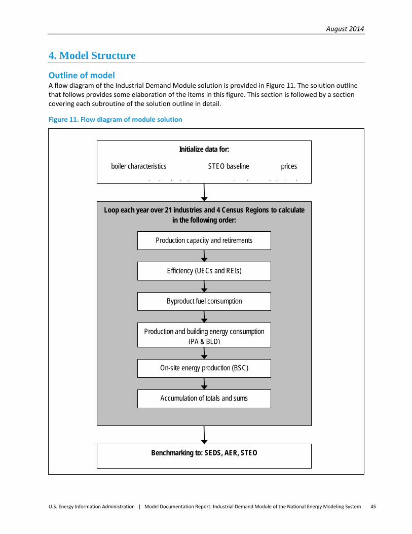
August 2014


4. Model Structure

Outline of model A flow diagram of the Industrial Demand Module solution is provided in Figure 11. The solution outline that follows provides some elaboration of the items in this figure. This section is followed by a section covering each subroutine of the solution outline in detail.

Figure 11. Flow diagram of module solution

Initialize data for:

boiler characteristics STEO baseline prices

i ( d ti ) ti h t i ti / t k

Loop each year over 21 industries and 4 Census Regions to calculate in the following order:

Production capacity and retirements

Efficiency (UECs and REIs)

Byproduct fuel consumption

Production and building energy consumption (PA & BLD)

On-site energy production (BSC)

Accumulation of totals and sums

Benchmarking to: SEDS, AER, STEO

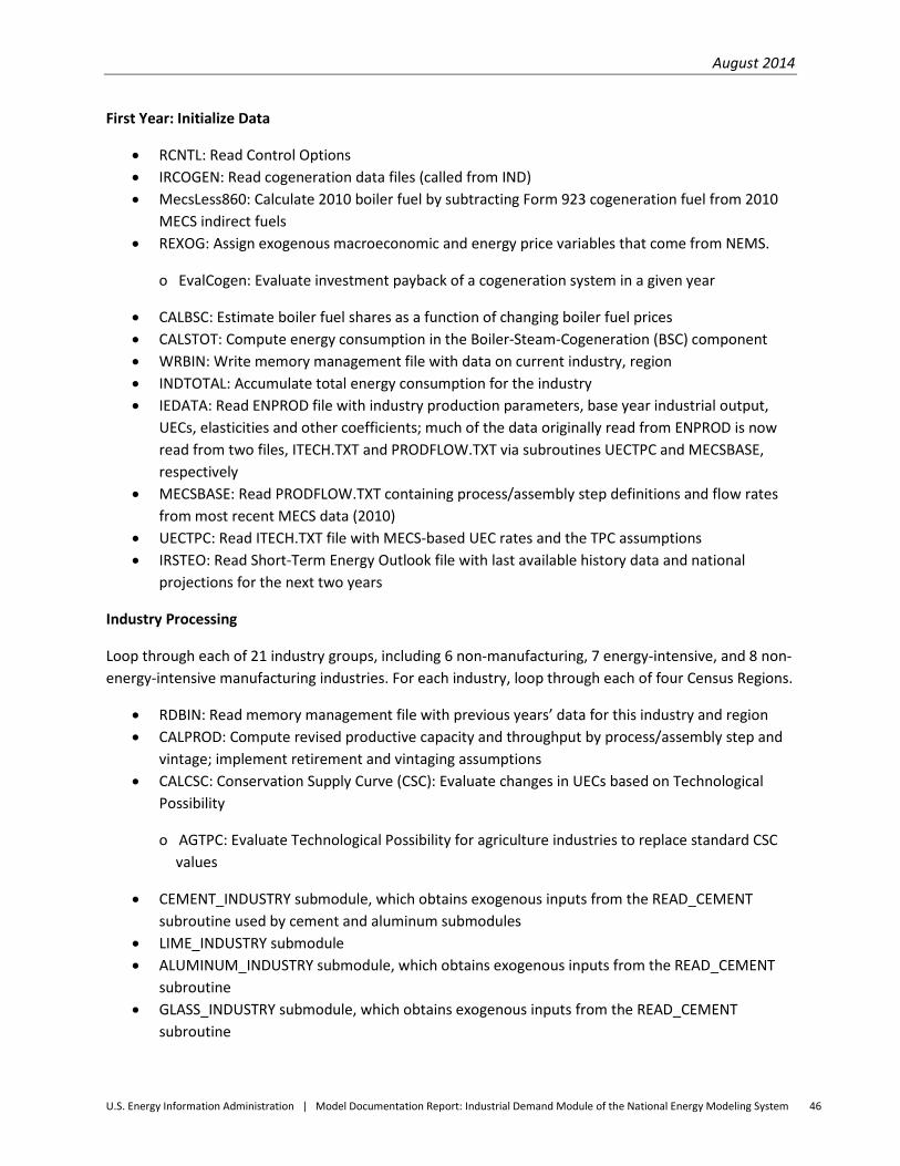
August 2014


First Year: Initialize Data

• RCNTL: Read Control Options • IRCOGEN: Read cogeneration data files (called from IND) • MecsLess860: Calculate 2010 boiler fuel by subtracting Form 923 cogeneration fuel from 2010

MECS indirect fuels • REXOG: Assign exogenous macroeconomic and energy price variables that come from NEMS.

o EvalCogen: Evaluate investment payback of a cogeneration system in a given year

• CALBSC: Estimate boiler fuel shares as a function of changing boiler fuel prices • CALSTOT: Compute energy consumption in the Boiler-Steam-Cogeneration (BSC) component • WRBIN: Write memory management file with data on current industry, region • INDTOTAL: Accumulate total energy consumption for the industry • IEDATA: Read ENPROD file with industry production parameters, base year industrial output,

UECs, elasticities and other coefficients; much of the data originally read from ENPROD is now read from two files, ITECH.TXT and PRODFLOW.TXT via subroutines UECTPC and MECSBASE, respectively

• MECSBASE: Read PRODFLOW.TXT containing process/assembly step definitions and flow rates from most recent MECS data (2010)

• UECTPC: Read ITECH.TXT file with MECS-based UEC rates and the TPC assumptions • IRSTEO: Read Short-Term Energy Outlook file with last available history data and national

projections for the next two years

Industry Processing

Loop through each of 21 industry groups, including 6 non-manufacturing, 7 energy-intensive, and 8 non-energy-intensive manufacturing industries. For each industry, loop through each of four Census Regions.

• RDBIN: Read memory management file with previous years’ data for this industry and region • CALPROD: Compute revised productive capacity and throughput by process/assembly step and

vintage; implement retirement and vintaging assumptions • CALCSC: Conservation Supply Curve (CSC): Evaluate changes in UECs based on Technological

Possibility

o AGTPC: Evaluate Technological Possibility for agriculture industries to replace standard CSC values

• CEMENT_INDUSTRY submodule, which obtains exogenous inputs from the READ_CEMENT subroutine used by cement and aluminum submodules

• LIME_INDUSTRY submodule • ALUMINUM_INDUSTRY submodule, which obtains exogenous inputs from the READ_CEMENT

subroutine • GLASS_INDUSTRY submodule, which obtains exogenous inputs from the READ_CEMENT

subroutine

August 2014


• CALBYPROD: Calculate consumption of byproduct fuels • CALPATOT: Compute consumption of energy in the process assembly component

o MOTORS: Compute consumption of electricity for machine-drive for end-use industries

• CALBTOT: Compute consumption of energy in the buildings component • CALGEN: Compute electricity generation for sale and internal use by fuel. Calculates steam for

cogeneration and estimates penetration of new builds. Calls the following routines:

o COGENT: Read cogeneration assumptions spreadsheet (first year) o SteamSeg: Assign fraction of steam load in current load segment for current industry o COGINIT: Initialize the cogeneration data arrays with capacity, generation, and fuel use data

National Summaries

• NATTOTAL: Accumulate total energy consumption over all industries • CONTAB: Accumulate aggregates for non-manufacturing heat and power

Apply exogenous adjustments and assign values to global variables

WEXOG • SEDS Benchmarking:

o SEDS years (through 2011): calculate regional benchmark factors as the ratio of actual consumption to model consumption for each fuel in four Census Regions. o Post SEDS Years (2012-on): optionally, multiply model consumption by the SEDS benchmark factors.

• Disaggregate energy consumption from four Census Regions to nine Census Divisions using shares from SEDS.

• Calibrate regional energy consumption to match the latest year of national-level history data (from the STEO file).

• STEO Benchmarking

o STEO years: calculate national benchmark factors as the ratio of model consumption for each fuel to the STEO projection for each fuel. o Post-STEO years: optionally, over the period 2013 to 2014, multiply model consumption by the STEO benchmark factors.

• Assign final results to NEMS variables.

Subroutines and equations This section provides the solution algorithms for the Industrial Demand Module. The order in which the equations are presented follows the logic of the Fortran source code very closely to facilitate an understanding of the code and its structure. All subroutines are run for each year (subscript y), industry (subscript i), and each of the four Census Regions (subscript r) unless otherwise indicated. For variables

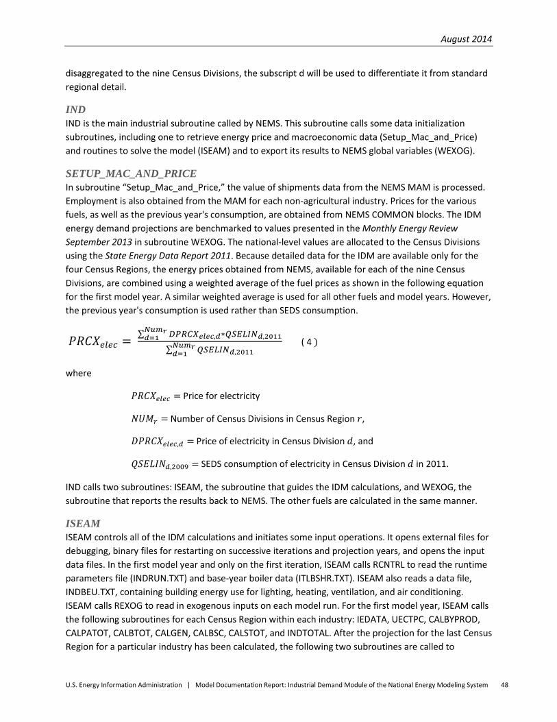
August 2014


disaggregated to the nine Census Divisions, the subscript d will be used to differentiate it from standard regional detail.

IND IND is the main industrial subroutine called by NEMS. This subroutine calls some data initialization subroutines, including one to retrieve energy price and macroeconomic data (Setup_Mac_and_Price) and routines to solve the model (ISEAM) and to export its results to NEMS global variables (WEXOG).

SETUP_MAC_AND_PRICE In subroutine “Setup_Mac_and_Price,” the value of shipments data from the NEMS MAM is processed. Employment is also obtained from the MAM for each non-agricultural industry. Prices for the various fuels, as well as the previous year's consumption, are obtained from NEMS COMMON blocks. The IDM energy demand projections are benchmarked to values presented in the Monthly Energy Review September 2013 in subroutine WEXOG. The national-level values are allocated to the Census Divisions using the State Energy Data Report 2011. Because detailed data for the IDM are available only for the four Census Regions, the energy prices obtained from NEMS, available for each of the nine Census Divisions, are combined using a weighted average of the fuel prices as shown in the following equation for the first model year. A similar weighted average is used for all other fuels and model years. However, the previous year's consumption is used rather than SEDS consumption.

𝑃𝑅𝐶𝑋𝑒𝑙𝑒𝑐 = ∑ 𝐷𝑃𝑅𝐶𝑋𝑒𝑙𝑒𝑐,𝑑∗𝑄𝑆𝐸𝐿𝐼𝑁𝑑,2011𝑁𝑢𝑚𝑟𝑑=1

∑ 𝑄𝑆𝐸𝐿𝐼𝑁𝑑,2011𝑁𝑢𝑚𝑟𝑑=1

( 4 )

where

𝑃𝑅𝐶𝑋𝑒𝑙𝑒𝑐 = Price for electricity

𝑁𝑈𝑀𝑟 = Number of Census Divisions in Census Region 𝑟,

𝐷𝑃𝑅𝐶𝑋𝑒𝑙𝑒𝑐,𝑑 = Price of electricity in Census Division 𝑑, and

𝑄𝑆𝐸𝐿𝐼𝑁𝑑,2009 = SEDS consumption of electricity in Census Division 𝑑 in 2011.

IND calls two subroutines: ISEAM, the subroutine that guides the IDM calculations, and WEXOG, the subroutine that reports the results back to NEMS. The other fuels are calculated in the same manner.

ISEAM ISEAM controls all of the IDM calculations and initiates some input operations. It opens external files for debugging, binary files for restarting on successive iterations and projection years, and opens the input data files. In the first model year and only on the first iteration, ISEAM calls RCNTRL to read the runtime parameters file (INDRUN.TXT) and base-year boiler data (ITLBSHR.TXT). ISEAM also reads a data file, INDBEU.TXT, containing building energy use for lighting, heating, ventilation, and air conditioning. ISEAM calls REXOG to read in exogenous inputs on each model run. For the first model year, ISEAM calls the following subroutines for each Census Region within each industry: IEDATA, UECTPC, CALBYPROD, CALPATOT, CALBTOT, CALGEN, CALBSC, CALSTOT, and INDTOTAL. After the projection for the last Census Region for a particular industry has been calculated, the following two subroutines are called to

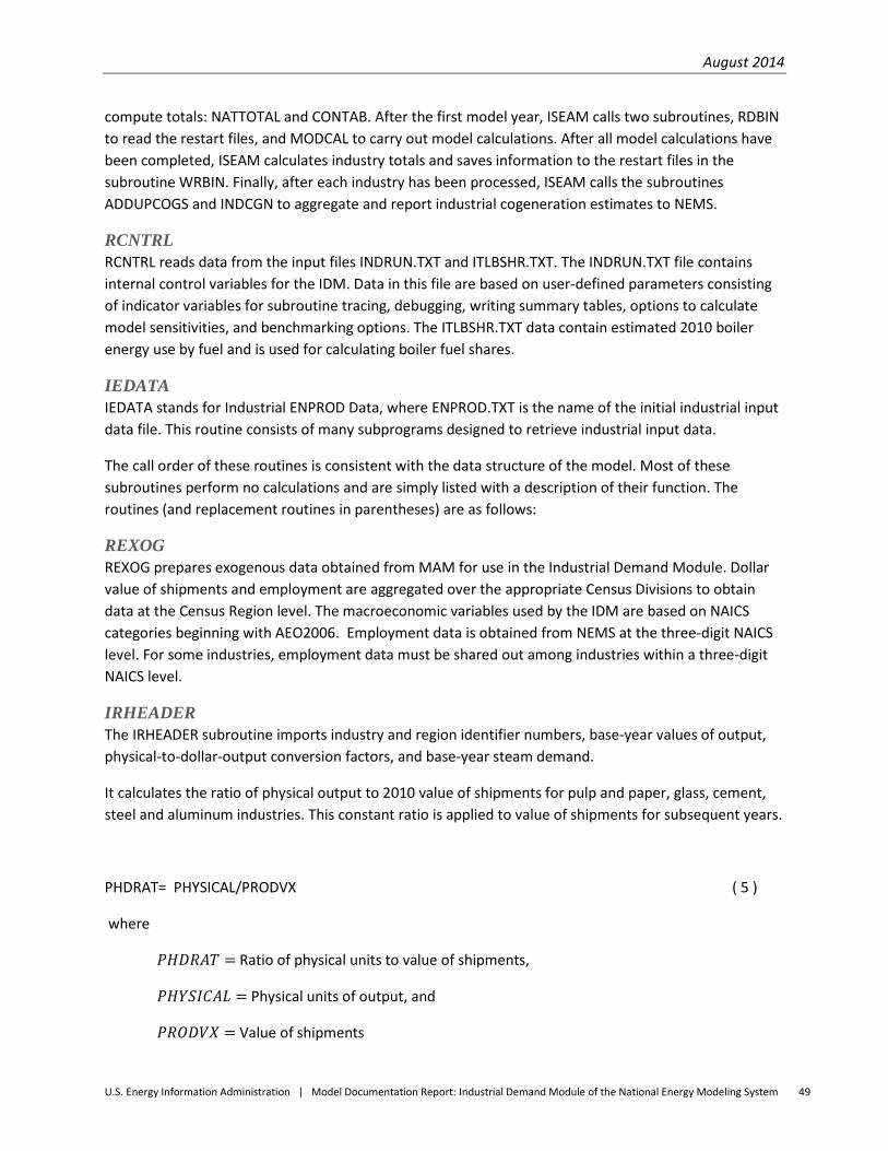
August 2014


compute totals: NATTOTAL and CONTAB. After the first model year, ISEAM calls two subroutines, RDBIN to read the restart files, and MODCAL to carry out model calculations. After all model calculations have been completed, ISEAM calculates industry totals and saves information to the restart files in the subroutine WRBIN. Finally, after each industry has been processed, ISEAM calls the subroutines ADDUPCOGS and INDCGN to aggregate and report industrial cogeneration estimates to NEMS.

RCNTRL RCNTRL reads data from the input files INDRUN.TXT and ITLBSHR.TXT. The INDRUN.TXT file contains internal control variables for the IDM. Data in this file are based on user-defined parameters consisting of indicator variables for subroutine tracing, debugging, writing summary tables, options to calculate model sensitivities, and benchmarking options. The ITLBSHR.TXT data contain estimated 2010 boiler energy use by fuel and is used for calculating boiler fuel shares.

IEDATA IEDATA stands for Industrial ENPROD Data, where ENPROD.TXT is the name of the initial industrial input data file. This routine consists of many subprograms designed to retrieve industrial input data.

The call order of these routines is consistent with the data structure of the model. Most of these subroutines perform no calculations and are simply listed with a description of their function. The routines (and replacement routines in parentheses) are as follows:

REXOG REXOG prepares exogenous data obtained from MAM for use in the Industrial Demand Module. Dollar value of shipments and employment are aggregated over the appropriate Census Divisions to obtain data at the Census Region level. The macroeconomic variables used by the IDM are based on NAICS categories beginning with AEO2006. Employment data is obtained from NEMS at the three-digit NAICS level. For some industries, employment data must be shared out among industries within a three-digit NAICS level.

IRHEADER The IRHEADER subroutine imports industry and region identifier numbers, base-year values of output, physical-to-dollar-output conversion factors, and base-year steam demand.

It calculates the ratio of physical output to 2010 value of shipments for pulp and paper, glass, cement, steel and aluminum industries. This constant ratio is applied to value of shipments for subsequent years.

PHDRAT= PHYSICAL/PRODVX ( 5 )

where

𝑃𝐻𝐷𝑅𝐴𝑇 = Ratio of physical units to value of shipments,

𝑃𝐻𝑌𝑆𝐼𝐶𝐴𝐿 = Physical units of output, and

𝑃𝑅𝑂𝐷𝑉𝑋 = Value of shipments

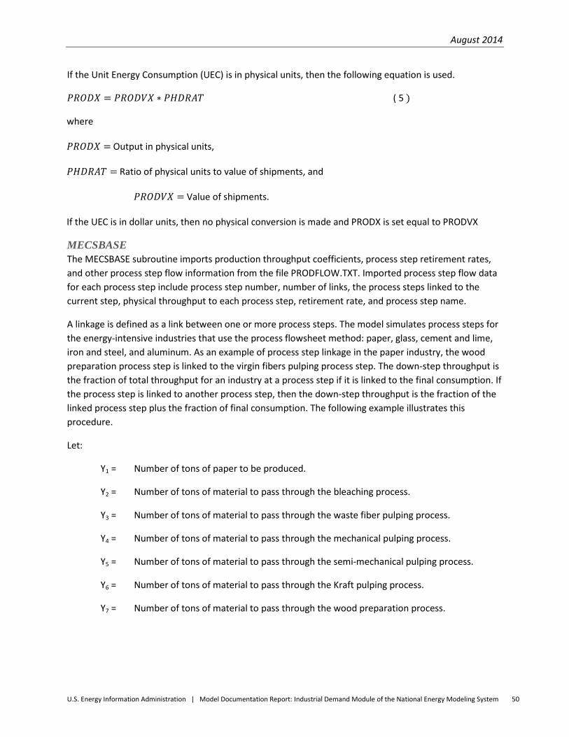
August 2014


If the Unit Energy Consumption (UEC) is in physical units, then the following equation is used.

𝑃𝑅𝑂𝐷𝑋 = 𝑃𝑅𝑂𝐷𝑉𝑋 ∗ 𝑃𝐻𝐷𝑅𝐴𝑇 ( 5 )

where

𝑃𝑅𝑂𝐷𝑋 = Output in physical units,

𝑃𝐻𝐷𝑅𝐴𝑇 = Ratio of physical units to value of shipments, and

𝑃𝑅𝑂𝐷𝑉𝑋 = Value of shipments.

If the UEC is in dollar units, then no physical conversion is made and PRODX is set equal to PRODVX

MECSBASE The MECSBASE subroutine imports production throughput coefficients, process step retirement rates, and other process step flow information from the file PRODFLOW.TXT. Imported process step flow data for each process step include process step number, number of links, the process steps linked to the current step, physical throughput to each process step, retirement rate, and process step name.

A linkage is defined as a link between one or more process steps. The model simulates process steps for the energy-intensive industries that use the process flowsheet method: paper, glass, cement and lime, iron and steel, and aluminum. As an example of process step linkage in the paper industry, the wood preparation process step is linked to the virgin fibers pulping process step. The down-step throughput is the fraction of total throughput for an industry at a process step if it is linked to the final consumption. If the process step is linked to another process step, then the down-step throughput is the fraction of the linked process step plus the fraction of final consumption. The following example illustrates this procedure.

Let:

Y1 = Number of tons of paper to be produced.

Y2 = Number of tons of material to pass through the bleaching process.

Y3 = Number of tons of material to pass through the waste fiber pulping process.

Y4 = Number of tons of material to pass through the mechanical pulping process.

Y5 = Number of tons of material to pass through the semi-mechanical pulping process.

Y6 = Number of tons of material to pass through the Kraft pulping process.

Y7 = Number of tons of material to pass through the wood preparation process.

August 2014


Then, we have the following:

Y1 = Output, in tons

Y2 = 0.502 Y1

Y3 = 0.317 (Y1 + Y2)

Y4 = 0.041 (Y1 + Y2)

Y5 = 0.028 (Y1 + Y2)

Y6 = 0.377 (Y1 + Y2)

Y7 = 1.689 (Y4 + Y5 + Y6)

If Y1 = 96 million tons of paper produced, then Y2 = 48, Y3 = 46, Y4 = 6.5, Y5 = 4, Y6 = 54, and Y7 = 109.

For the above example, there are 109 million tons of output from the wood preparation process and 46 million tons of output from the waste fiber pulping process. Of the 109 million tons of material passing through the wood preparation process, 10 million tons flow through mechanical pulping, 7 million tons into semi-mechanical pulping, and 92 million tons into the Kraft pulping process. In the IDM, these calculations are performed in an input-output formulation (see CALPROD below for more information).

Physical throughput is obtained for three vintages: old, middle, and new. Old vintage is defined as any capital installed in or before 2010. Middle vintage includes installations from 2007 to the year prior to the current projection year. New vintage includes any capital installed in the current projection year.

In summary, the following subroutines collect data from the input files.

ISEAM

Get building energy use data including lighting, HVAC, facility support, and onsite transportation from INDBEU.TXT.

IRBSCBYP

Get byproduct fuel information for the boiler/steam/cogeneration component. These data consist of fuel identifier numbers of steam intensity values.

RDCNTL

Read INDRUN.TXT and ITLBSHR.TXT. The latter contains base year boiler-fuel use and is used to calculate boiler-fuel shares. Biomass data is retrieved in the IRBSCBYP routine.

IRCOGEN

Get cogeneration information from file EXSTCAP.TXT, including capacity, generation, fuel use, and thermal output from 1990 through 2008. Get corresponding data for planned units from file PLANCAP.TXT.

IRSTEPBYP

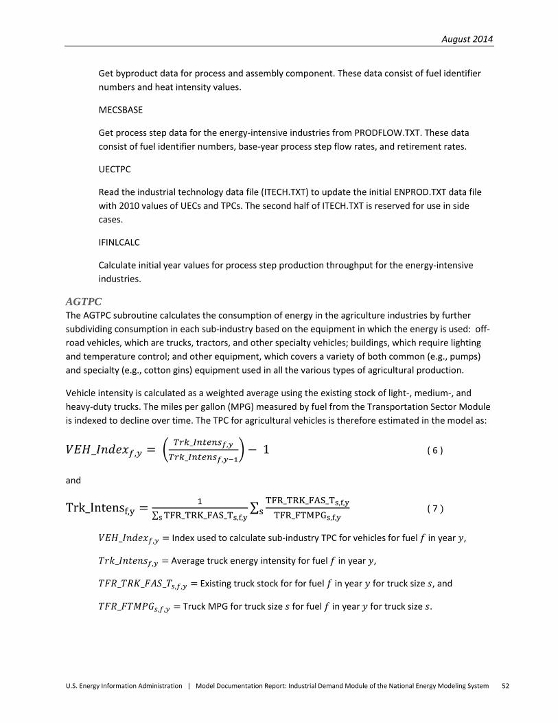
August 2014


Get byproduct data for process and assembly component. These data consist of fuel identifier numbers and heat intensity values.

MECSBASE

Get process step data for the energy-intensive industries from PRODFLOW.TXT. These data consist of fuel identifier numbers, base-year process step flow rates, and retirement rates.

UECTPC

Read the industrial technology data file (ITECH.TXT) to update the initial ENPROD.TXT data file with 2010 values of UECs and TPCs. The second half of ITECH.TXT is reserved for use in side cases.

IFINLCALC

Calculate initial year values for process step production throughput for the energy-intensive industries.

AGTPC The AGTPC subroutine calculates the consumption of energy in the agriculture industries by further subdividing consumption in each sub-industry based on the equipment in which the energy is used: off-road vehicles, which are trucks, tractors, and other specialty vehicles; buildings, which require lighting and temperature control; and other equipment, which covers a variety of both common (e.g., pumps) and specialty (e.g., cotton gins) equipment used in all the various types of agricultural production.

Vehicle intensity is calculated as a weighted average using the existing stock of light-, medium-, and heavy-duty trucks. The miles per gallon (MPG) measured by fuel from the Transportation Sector Module is indexed to decline over time. The TPC for agricultural vehicles is therefore estimated in the model as:

𝑉𝐸𝐻_𝐼𝑛𝑑𝑒𝑥𝑓,𝑦 = � 𝑇𝑟𝑘_𝐼𝑛𝑡𝑒𝑛𝑠𝑓,𝑦

𝑇𝑟𝑘_𝐼𝑛𝑡𝑒𝑛𝑠𝑓,𝑦−1� − 1 ( 6 )

and

Trk_Intensf,y = 1∑ TFR_TRK_FAS_Ts,f,ys

∑ TFR_TRK_FAS_Ts,f,y

TFR_FTMPGs,f,ys ( 7 )

𝑉𝐸𝐻_𝐼𝑛𝑑𝑒𝑥𝑓,𝑦 = Index used to calculate sub-industry TPC for vehicles for fuel 𝑓 in year 𝑦,

𝑇𝑟𝑘_𝐼𝑛𝑡𝑒𝑛𝑠𝑓,𝑦 = Average truck energy intensity for fuel 𝑓 in year 𝑦,

𝑇𝐹𝑅_𝑇𝑅𝐾_𝐹𝐴𝑆_𝑇𝑠,𝑓,𝑦 = Existing truck stock for for fuel 𝑓 in year 𝑦 for truck size 𝑠, and

𝑇𝐹𝑅_𝐹𝑇𝑀𝑃𝐺𝑠,𝑓,𝑦 = Truck MPG for truck size 𝑠 for fuel 𝑓 in year 𝑦 for truck size 𝑠.

August 2014


Building energy intensity is calculated using an index of heating, lighting, and building shells retrieved from the Commercial Demand Module for warehouses, since this building type is most similar to the types of buildings used in agricultural production. The shares for these three energy users are based on data analysis commissioned by EIA29 and shown in

Table 5. The TPC for agricultural buildings is estimated in the model as:

𝐵𝐿𝐷𝐼𝑛𝑑𝑒𝑥𝑟,1,𝑦 = �𝑊𝐻𝑆𝐸𝐻𝑒𝑎𝑡𝐼𝑛𝑑𝑒𝑥𝑟,𝑓,𝑦

𝑊𝐻𝑆𝐸𝐻𝑒𝑎𝑡𝐼𝑛𝑑𝑒𝑥𝑟,𝑓,𝑦−1� − 1 ( 8 )

𝐵𝐿𝐷_𝐼𝑛𝑑𝑒𝑥𝑟,2,𝑦 = � 𝑊𝐻𝑆𝐸_𝐿𝑖𝑔ℎ𝑡𝐼𝑛𝑑𝑒𝑥𝑟,𝑓,𝑦

𝑊𝐻𝑆𝐸_𝐿𝑖𝑔ℎ𝑡𝐼𝑛𝑑𝑒𝑥𝑟,𝑓,𝑦−1� − 1 ( 9 )

𝐵𝐿𝐷𝐼𝑛𝑑𝑒𝑥𝑟,3,𝑦 = �𝑊𝐻𝑆𝐸𝑆ℎ𝑒𝑙𝑙𝐼𝑛𝑑𝑒𝑥𝑟,𝑓,𝑦

𝑊𝐻𝑆𝐸𝑆ℎ𝑒𝑙𝑙𝐼𝑛𝑑𝑒𝑥𝑟,𝑓,,𝑦−1� − 1 ( 10 )

where

𝐵𝐿𝐷_𝐼𝑛𝑑𝑒𝑥𝑟,k,,𝑦 Index, before weighting for heating equipment (k=1), lighting equipment (k=2) or building shells (k=3), used to calculate sub-industry TPC for buildings for region 𝑟 in year 𝑦

𝑊𝐻𝑆𝐸_𝐻𝑒𝑎𝑡𝐼𝑛𝑑𝑒𝑥𝑟,𝑓,𝑦 = Composite of warehouse energy consumption in heating equipment retrieved from the Commercial Demand Module in region 𝑟 for fuel 𝑓 in year 𝑦,

𝑊𝐻𝑆𝐸_𝐿𝑖𝑔ℎ𝑡𝐼𝑛𝑑𝑒𝑥𝑟,𝑓,𝑦 = Composite of warehouse energy consumption in lighting equipment retrieved from the Commercial Demand Module in region 𝑟 for fuel 𝑓 in year 𝑦,

𝑊𝐻𝑆𝐸_𝑆ℎ𝑒𝑙𝑙𝐼𝑛𝑑𝑒𝑥𝑟,𝑓,𝑦 = Composite of warehouse energy consumption in building shells retrieved from the Commercial Demand Module in region 𝑟 for fuel 𝑓 in year 𝑦

Irrigation intensity is computed much the same way as the building intensity, relying on

𝑊𝐻𝑆𝐸_𝑉𝑒𝑛𝑡𝐼𝑛𝑑𝑒𝑥𝑟,𝑓,𝑦 instead:

𝐼𝑅𝑅_𝐼𝑛𝑑𝑒𝑥𝑟,𝑓,𝑦 = � 𝑊𝐻𝑆𝐸_𝑉𝑒𝑛𝑡𝐼𝑛𝑑𝑒𝑥𝑟,𝑓,𝑦

𝑊𝐻𝑆𝐸_𝑉𝑒𝑛𝑡𝐼𝑛𝑑𝑒𝑥𝑟,𝑓,𝑦−1� − 1 ( 11 )

29 SRA International, “Report on the Analysis and Modeling Approach to Characterize and Estimate Fuel Use by End-Use Applications in the Agriculture and Construction Industries,” unpublished report prepared for the U.S. Energy Information Administration, March 2011.

August 2014


where

𝑊𝐻𝑆𝐸_𝑉𝑒𝑛𝑡𝐼𝑛𝑑𝑒𝑥𝑟,𝑓,𝑦 = Composite of warehouse energy consumption in building vents retrieved from the Commercial Demand Module in region 𝑟 for fuel 𝑓 in year 𝑦

Table 5. Building weights for TPC index by fuel

Equipment Type Heating Lighting Shell Electricity 0.25 0.25 0.50 Natural gas 0.25 0.00 0.75 Distillate 0.25 0.00 0.75 NGL 0.25 0.00 0.75 Motor Gasoline 0.25 0.00 0.75 Source: CDM Documentation.

Other equipment is directly indexed to other warehouse equipment using a fourth composite retrieved from the Commercial Demand Module.30

CONTPC The construction industry (NAICS 236-238) encompasses all forms of residential, commercial, and industrial construction activities. It includes road and bridge construction, laying (and consumption) of asphalt, as well as all contractor-related activities. The consumption sector is modeled as one sector, but comprises three subsectors, or functional groups. Functional group weightings are derived by region and fuel, and these are applied to indices of vehicle use derived from the Transportation Demand Module (TDM). These indices of vehicle use are similar to the ones used for agriculture; the mix of vehicles is different. In addition, an investment index of state and local highway investment is the primary factor in determining asphalt demand provided by the Macroeconomic Activity Module (MAM).

The energy demanded for any given fuel is dependent on the value of output in the construction sector, as follows:

𝑄𝑟,𝑓,𝑦 = 𝐶𝑂𝑁𝑆𝑇𝑅𝑟,𝑦 ∗ 𝑈𝐸𝐶𝑟,𝑓,𝑦 ( 12 )

𝑈𝐸𝐶𝑟,𝑓,𝑦 = 𝑈𝐸𝐶𝑟,𝑓,𝑦−1 ∗ �1 + 𝑇𝑃𝐶𝑓,𝑦� ( 13 )

where

𝑄𝑟,𝑓,𝑦 = quantity demanded in region r of fuel f for year y

𝐶𝑂𝑁𝑆𝑇𝑅𝑟,𝑦 = Construction shipments from the MAM for region r and year y

30Details of the three warehouse energy consumption variables can be found in U.S. Energy Information Administration, Documentation of the Commercial Demand Module (CDM), DOE/EIA-M066(2013), Washington, DC, July 2011, pg. 16-39.

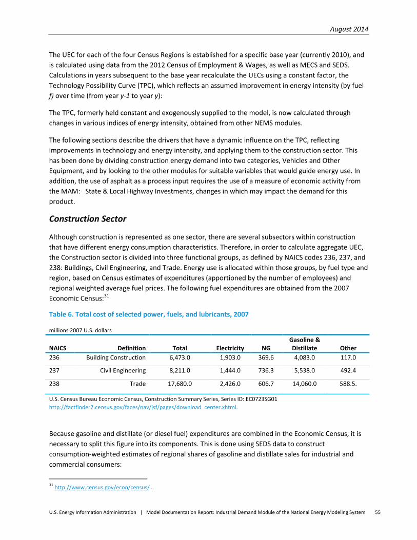
August 2014


The UEC for each of the four Census Regions is established for a specific base year (currently 2010), and is calculated using data from the 2012 Census of Employment & Wages, as well as MECS and SEDS. Calculations in years subsequent to the base year recalculate the UECs using a constant factor, the Technology Possibility Curve (TPC), which reflects an assumed improvement in energy intensity (by fuel f) over time (from year y-1 to year y):

The TPC, formerly held constant and exogenously supplied to the model, is now calculated through changes in various indices of energy intensity, obtained from other NEMS modules.

The following sections describe the drivers that have a dynamic influence on the TPC, reflecting improvements in technology and energy intensity, and applying them to the construction sector. This has been done by dividing construction energy demand into two categories, Vehicles and Other Equipment, and by looking to the other modules for suitable variables that would guide energy use. In addition, the use of asphalt as a process input requires the use of a measure of economic activity from the MAM: State & Local Highway Investments, changes in which may impact the demand for this product.

Construction Sector

Although construction is represented as one sector, there are several subsectors within construction that have different energy consumption characteristics. Therefore, in order to calculate aggregate UEC, the Construction sector is divided into three functional groups, as defined by NAICS codes 236, 237, and 238: Buildings, Civil Engineering, and Trade. Energy use is allocated within those groups, by fuel type and region, based on Census estimates of expenditures (apportioned by the number of employees) and regional weighted average fuel prices. The following fuel expenditures are obtained from the 2007 Economic Census:31

Table 6. Total cost of selected power, fuels, and lubricants, 2007

millions 2007 U.S. dollars

NAICS Definition Total Electricity NG Gasoline & Distillate Other

236 Building Construction 6,473.0 1,903.0 369.6 4,083.0 117.0

237 Civil Engineering 8,211.0 1,444.0 736.3 5,538.0 492.4

238 Trade 17,680.0 2,426.0 606.7 14,060.0 588.5.

U.S. Census Bureau Economic Census, Construction Summary Series, Series ID: EC0723SG01 http://factfinder2.census.gov/faces/nav/jsf/pages/download_center.xhtml.

Because gasoline and distillate (or diesel fuel) expenditures are combined in the Economic Census, it is necessary to split this figure into its components. This is done using SEDS data to construct consumption-weighted estimates of regional shares of gasoline and distillate sales for industrial and commercial consumers:

31 http://www.census.gov/econ/census/ .

http://factfinder2.census.gov/faces/nav/jsf/pages/download_center.xhtml

http://www.census.gov/econ/census/

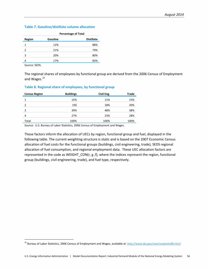
August 2014


Table 7. Gasoline/distillate volume allocation

Percentage of Total

Region Gasoline Distillate

1 12% 88%

2 21% 79%

3 20% 80%

4 17% 83% Source: SEDS.

The regional shares of employees by functional group are derived from the 2006 Census of Employment and Wages.32

Table 8. Regional share of employees, by functional group

Census Region Buildings Civil Eng. Trade

1 15% 11% 15%

2 19$ 18% 20%

3 39% 48% 38%

4 27% 23% 28%

Total 100% 100% 100% Source: U.S. Bureau of Labor Statistics, 2006 Census of Employment and Wages.

These factors inform the allocation of UECs by region, functional group and fuel, displayed in the following table. The current weighting structure is static and is based on the 2007 Economic Census allocation of fuel costs for the functional groups (buildings, civil engineering, trade), SEDS regional allocation of fuel consumption, and regional employment data. These UEC allocation factors are represented in the code as WEIGHT_CON(r, g ,f), where the indices represent the region, functional group (buildings, civil engineering, trade), and fuel type, respectively.

32 Bureau of Labor Statistics, 2006 Census of Employment and Wages, available at http://www.bls.gov/cew/cewbultn06.htm/

http://www.bls.gov/cew/cewbultn06.htm/

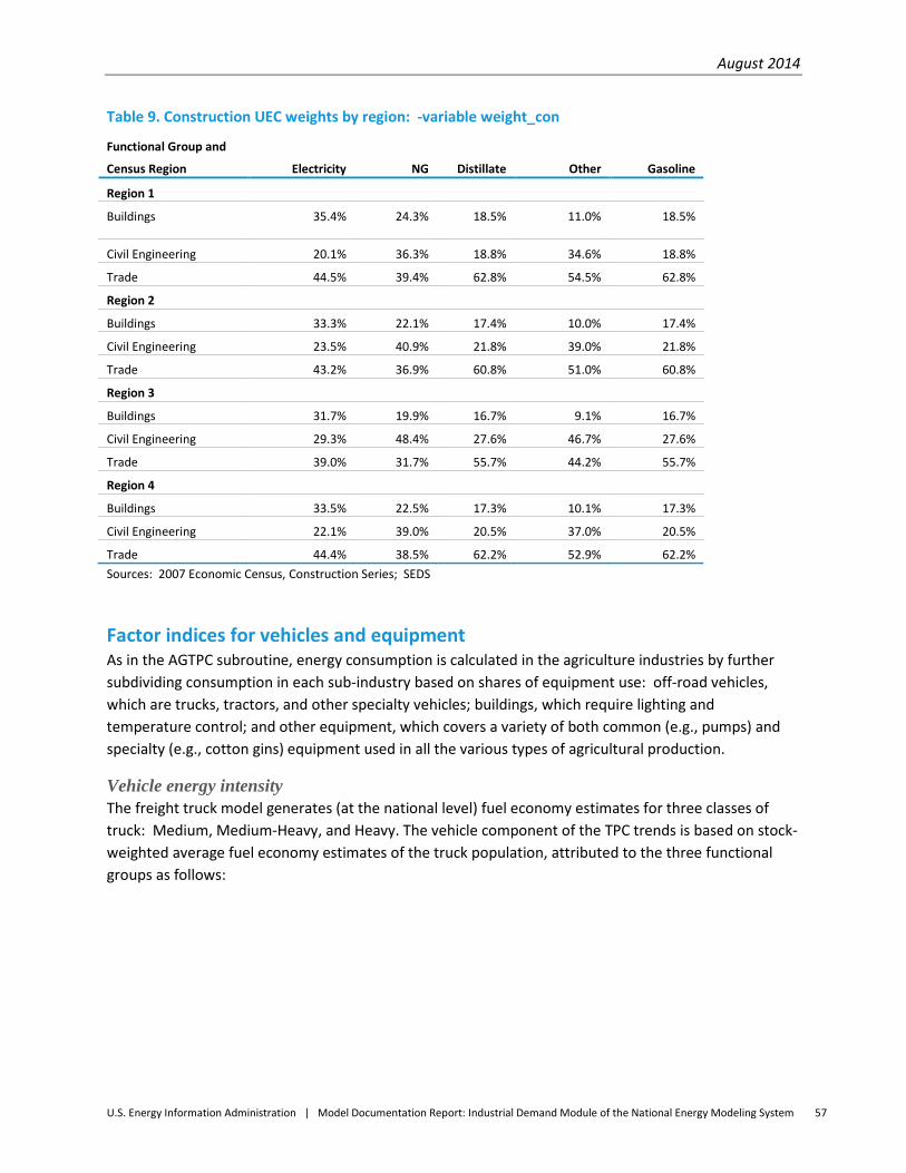
August 2014


Table 9. Construction UEC weights by region: -variable weight_con Functional Group and

Census Region Electricity NG Distillate Other Gasoline

Region 1

Buildings 35.4% 24.3% 18.5% 11.0% 18.5%

Civil Engineering 20.1% 36.3% 18.8% 34.6% 18.8%

Trade 44.5% 39.4% 62.8% 54.5% 62.8%

Region 2

Buildings 33.3% 22.1% 17.4% 10.0% 17.4%


Trade 43.2% 36.9% 60.8% 51.0% 60.8%

Region 3

Buildings 31.7% 19.9% 16.7% 9.1% 16.7%


Trade 39.0% 31.7% 55.7% 44.2% 55.7%

Region 4

Buildings 33.5% 22.5% 17.3% 10.1% 17.3%


Trade 44.4% 38.5% 62.2% 52.9% 62.2% Sources: 2007 Economic Census, Construction Series; SEDS

Factor indices for vehicles and equipment As in the AGTPC subroutine, energy consumption is calculated in the agriculture industries by further subdividing consumption in each sub-industry based on shares of equipment use: off-road vehicles, which are trucks, tractors, and other specialty vehicles; buildings, which require lighting and temperature control; and other equipment, which covers a variety of both common (e.g., pumps) and specialty (e.g., cotton gins) equipment used in all the various types of agricultural production.

Vehicle energy intensity The freight truck model generates (at the national level) fuel economy estimates for three classes of truck: Medium, Medium-Heavy, and Heavy. The vehicle component of the TPC trends is based on stock-weighted average fuel economy estimates of the truck population, attributed to the three functional groups as follows:

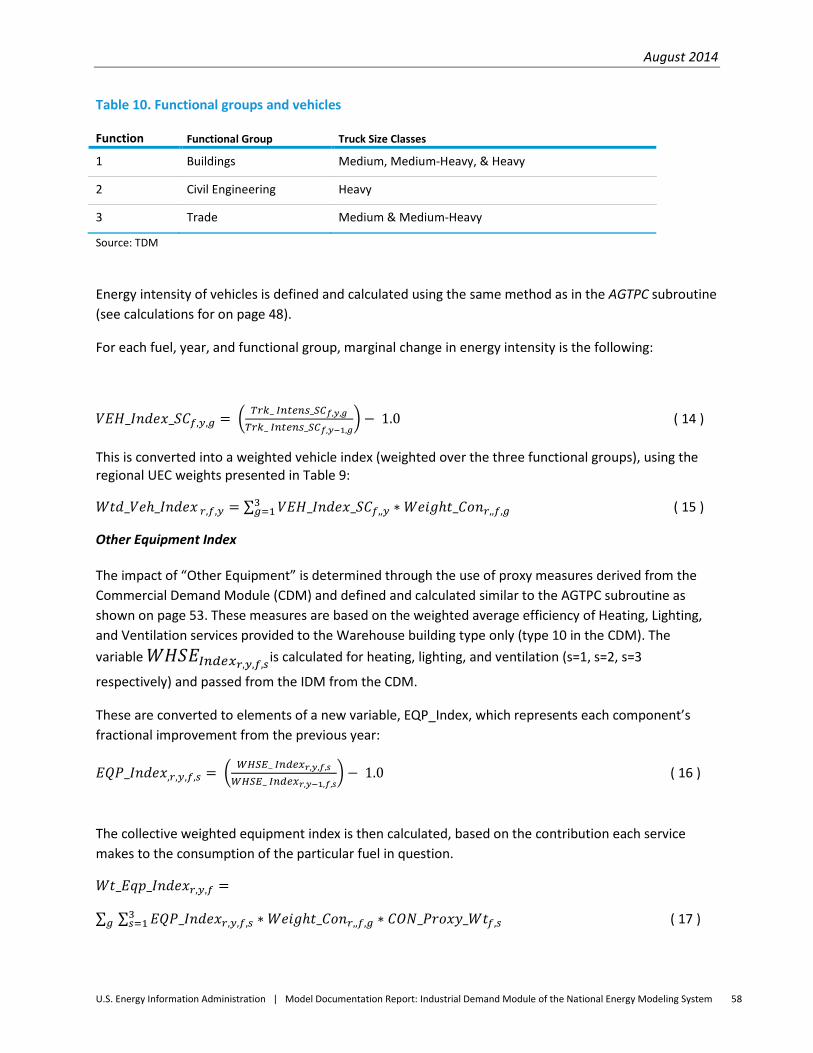
August 2014


Table 10. Functional groups and vehicles

Function Functional Group Truck Size Classes

1 Buildings Medium, Medium-Heavy, & Heavy

2 Civil Engineering Heavy

3 Trade Medium & Medium-Heavy

Source: TDM

Energy intensity of vehicles is defined and calculated using the same method as in the AGTPC subroutine (see calculations for on page 48).

For each fuel, year, and functional group, marginal change in energy intensity is the following:

𝑉𝐸𝐻_𝐼𝑛𝑑𝑒𝑥_𝑆𝐶𝑓,𝑦,𝑔 = � 𝑇𝑟𝑘_ 𝐼𝑛𝑡𝑒𝑛𝑠_𝑆𝐶𝑓,𝑦,𝑔

𝑇𝑟𝑘_ 𝐼𝑛𝑡𝑒𝑛𝑠_𝑆𝐶𝑓,𝑦−1,𝑔� − 1.0 ( 14 )

This is converted into a weighted vehicle index (weighted over the three functional groups), using the regional UEC weights presented in Table 9:

𝑊𝑡𝑑_𝑉𝑒ℎ_𝐼𝑛𝑑𝑒𝑥 𝑟,𝑓,𝑦 = ∑ 𝑉𝐸𝐻_𝐼𝑛𝑑𝑒𝑥_𝑆𝐶𝑓,,𝑦 ∗ 𝑊𝑒𝑖𝑔ℎ𝑡_𝐶𝑜𝑛𝑟,,𝑓,𝑔3𝑔=1 ( 15 )

Other Equipment Index

The impact of “Other Equipment” is determined through the use of proxy measures derived from the Commercial Demand Module (CDM) and defined and calculated similar to the AGTPC subroutine as shown on page 53. These measures are based on the weighted average efficiency of Heating, Lighting, and Ventilation services provided to the Warehouse building type only (type 10 in the CDM). The variable 𝑊𝐻𝑆𝐸𝐼𝑛𝑑𝑒𝑥𝑟,𝑦,𝑓,𝑠 is calculated for heating, lighting, and ventilation (s=1, s=2, s=3

respectively) and passed from the IDM from the CDM.

These are converted to elements of a new variable, EQP_Index, which represents each component’s fractional improvement from the previous year:

𝐸𝑄𝑃_𝐼𝑛𝑑𝑒𝑥,𝑟,𝑦,𝑓,𝑠 = � 𝑊𝐻𝑆𝐸_ 𝐼𝑛𝑑𝑒𝑥𝑟,𝑦,𝑓,𝑠

𝑊𝐻𝑆𝐸_ 𝐼𝑛𝑑𝑒𝑥𝑟,𝑦−1,𝑓,𝑠� − 1.0 ( 16 )

The collective weighted equipment index is then calculated, based on the contribution each service makes to the consumption of the particular fuel in question.

𝑊𝑡_𝐸𝑞𝑝_𝐼𝑛𝑑𝑒𝑥𝑟,𝑦,𝑓 =

∑ ∑ 𝐸𝑄𝑃_𝐼𝑛𝑑𝑒𝑥𝑟,𝑦,𝑓,𝑠 ∗ 𝑊𝑒𝑖𝑔ℎ𝑡_𝐶𝑜𝑛𝑟,,𝑓,𝑔 ∗ 𝐶𝑂𝑁_𝑃𝑟𝑜𝑥𝑦_𝑊𝑡𝑓,𝑠3𝑠=1𝑔 ( 17 )

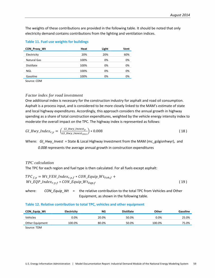
August 2014


The weights of these contributions are provided in the following table. It should be noted that only electricity demand contains contributions from the lighting and ventilation indices.

Table 11. Fuel use weights for buildings

CON_Proxy_Wt Heat Light Vent

Electricity 20% 20% 60%

Natural Gas 100% 0% 0%

Distillate 100% 0% 0%

NGL 100% 0% 0%

Gasoline 100% 0% 0% Source: CDM

Factor index for road investment One additional index is necessary for the construction industry for asphalt and road oil consumption. Asphalt is a process input, and is considered to be more closely linked to the MAM’s estimate of state and local highway expenditures. Accordingly, this approach considers the annual growth in highway spending as a share of total construction expenditures, weighted by the vehicle energy intensity index to moderate the overall impact on the TPC. The highway index is represented as follows:

𝐺𝐼_𝐻𝑤𝑦_𝐼𝑛𝑑𝑒𝑥𝑟,𝑦 = � 𝐺𝐼_𝐻𝑤𝑦_𝐼𝑛𝑣𝑒𝑠𝑡𝑦𝐺𝐼_𝐻𝑤𝑦_𝐼𝑛𝑣𝑒𝑠𝑡2011

� ∗ 0.008 ( 18 )

Where: GI_Hwy_Invest = State & Local Highway Investment from the MAM (mc_gslgisnhwyr), and

0.008 represents the average annual growth in construction expenditures

TPC calculation The TPC for each region and fuel type is then calculated. For all fuels except asphalt:

𝑇𝑃𝐶 𝑓,𝑦 = 𝑊𝑡_𝑉𝐸𝐻_𝐼𝑛𝑑𝑒𝑥𝑟,𝑦,𝑓 ∗ 𝐶𝑂𝑁_𝐸𝑞𝑢𝑖𝑝_𝑊𝑡𝑉𝑒ℎ,𝑓 + 𝑊𝑡_𝐸𝑄𝑃_𝐼𝑛𝑑𝑒𝑥𝑟,𝑦,𝑓 ∗ 𝐶𝑂𝑁_𝐸𝑞𝑢𝑖𝑝_𝑊𝑡𝐸𝑞𝑝,𝑓 ( 19 )

where: CON_Equip_Wt = the relative contribution to the total TPC from Vehicles and Other Equipment, as shown in the following table.

Table 12. Relative contribution to total TPC, vehicles and other equipment

CON_Equip_Wt Electricity NG Distillate Other Gasoline Vehicles 0.0% 20.0% 50.0% 0.0% 25.0% Other Equipment 100.0% 80.0% 50.0% 100.0% 75.0% Source: TDM

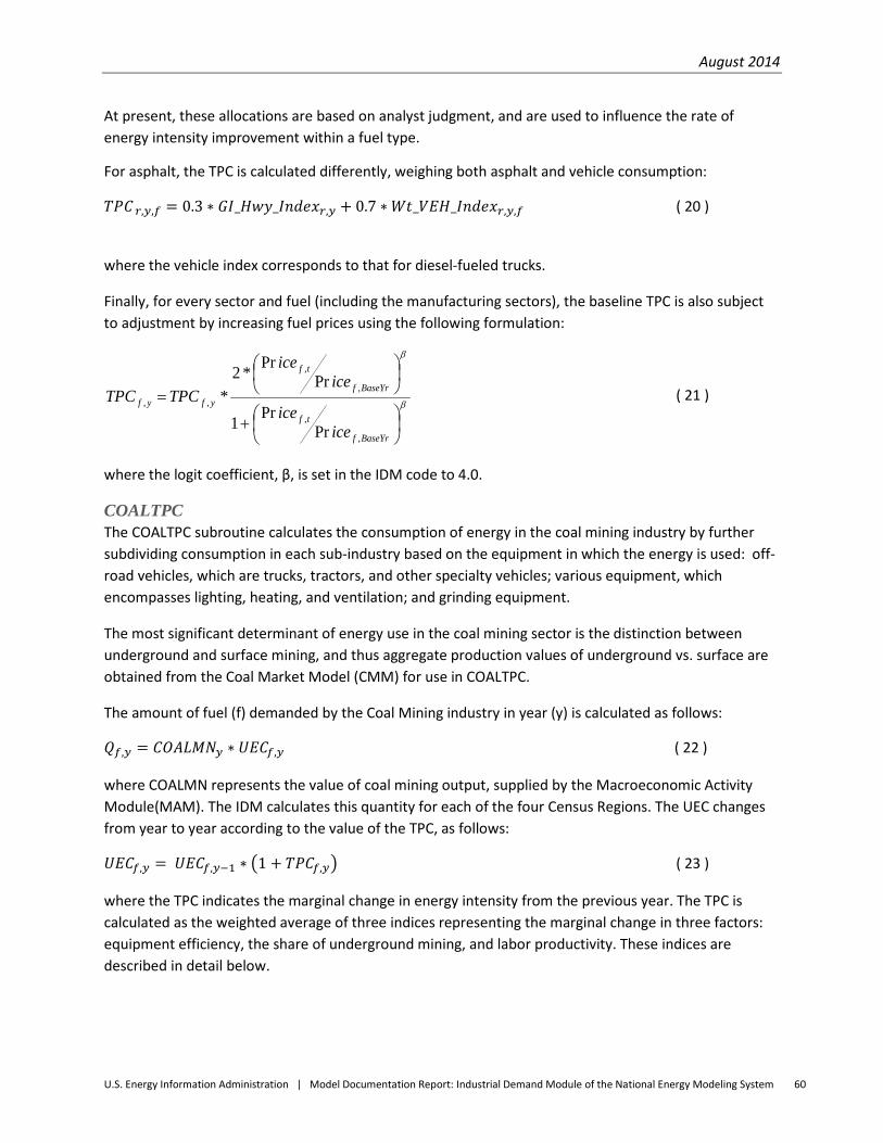
August 2014


At present, these allocations are based on analyst judgment, and are used to influence the rate of energy intensity improvement within a fuel type.

For asphalt, the TPC is calculated differently, weighing both asphalt and vehicle consumption:

𝑇𝑃𝐶 𝑟,𝑦,𝑓 = 0.3 ∗ 𝐺𝐼_𝐻𝑤𝑦_𝐼𝑛𝑑𝑒𝑥𝑟,𝑦 + 0.7 ∗𝑊𝑡_𝑉𝐸𝐻_𝐼𝑛𝑑𝑒𝑥𝑟,𝑦,𝑓 ( 20 )

where the vehicle index corresponds to that for diesel-fueled trucks.

Finally, for every sector and fuel (including the manufacturing sectors), the baseline TPC is also subject to adjustment by increasing fuel prices using the following formulation:

β

β

+

=

BaseYrf

tf

BaseYrf

tf

yfyf

iceice

iceice

TPCTPC

,

,

,

,

,,

PrPr1

PrPr*2

* ( 21 )

where the logit coefficient, β, is set in the IDM code to 4.0.

COALTPC The COALTPC subroutine calculates the consumption of energy in the coal mining industry by further subdividing consumption in each sub-industry based on the equipment in which the energy is used: off-road vehicles, which are trucks, tractors, and other specialty vehicles; various equipment, which encompasses lighting, heating, and ventilation; and grinding equipment.

The most significant determinant of energy use in the coal mining sector is the distinction between underground and surface mining, and thus aggregate production values of underground vs. surface are obtained from the Coal Market Model (CMM) for use in COALTPC.

The amount of fuel (f) demanded by the Coal Mining industry in year (y) is calculated as follows:

𝑄𝑓,𝑦 = 𝐶𝑂𝐴𝐿𝑀𝑁𝑦 ∗ 𝑈𝐸𝐶𝑓,𝑦 ( 22 )

where COALMN represents the value of coal mining output, supplied by the Macroeconomic Activity Module(MAM). The IDM calculates this quantity for each of the four Census Regions. The UEC changes from year to year according to the value of the TPC, as follows:

𝑈𝐸𝐶𝑓,𝑦 = 𝑈𝐸𝐶𝑓,𝑦−1 ∗ �1 + 𝑇𝑃𝐶𝑓,𝑦� ( 23 )

where the TPC indicates the marginal change in energy intensity from the previous year. The TPC is calculated as the weighted average of three indices representing the marginal change in three factors: equipment efficiency, the share of underground mining, and labor productivity. These indices are described in detail below.

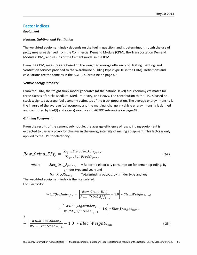
August 2014


Factor indices Equipment

Heating, Lighting, and Ventilation

The weighted equipment index depends on the fuel in question, and is determined through the use of proxy measures derived from the Commercial Demand Module (CDM), the Transportation Demand Module (TDM), and results of the Cement model in the IDM.

From the CDM, measures are based on the weighted average efficiency of Heating, Lighting, and Ventilation services provided to the Warehouse building type (type 10 in the CDM). Definitions and calculations are the same as in the AGTPC subroutine on page 49.

Vehicle Energy Intensity

From the TDM, the freight truck model generates (at the national level) fuel economy estimates for three classes of truck: Medium, Medium-Heavy, and Heavy. The contribution to the TPC is based on stock-weighted average fuel economy estimates of the truck population. The average energy intensity is the inverse of the average fuel economy and the marginal change in vehicle energy intensity is defined and computed by fuel(f) and year(y) exactly as in AGTPC subroutine on page 48 .

Grinding Equipment

From the results of the cement submodule, the average efficiency of raw grinding equipment is extracted to use as a proxy for changes in the energy intensity of mining equipment. This factor is only applied to the TPC for electricity.

𝑅𝑎𝑤_𝐺𝑟𝑖𝑛𝑑_𝐸𝑓𝑓𝑦 = ∑ 𝐸𝑙𝑒𝑐_𝑈𝑠𝑒_𝑅𝑝𝑡𝑡𝑦𝑝𝑒,𝑦𝑡𝑦𝑝𝑒

∑ 𝑇𝑜𝑡_𝑃𝑟𝑜𝑑𝐺𝑡𝑦𝑝𝑒,𝑦𝑡𝑦𝑝𝑒 ( 24 )

where: Elec_Use_Rpttype,y = Reported electricity consumption for cement grinding, by grinder type and year; and

Tot_ProdGtype,y= Total grinding output, by grinder type and year The weighted equipment index is then calculated. For Electricity:

𝑊𝑡_𝐸𝑄𝑃_𝐼𝑛𝑑𝑒𝑥𝑓,𝑦 = �𝑅𝑎𝑤_𝐺𝑟𝑖𝑛𝑑_𝐸𝑓𝑓𝑦𝑅𝑎𝑤_𝐺𝑟𝑖𝑛𝑑_𝐸𝑓𝑓𝑦−1

− 1.0� ∗ 𝐸𝑙𝑒𝑐_𝑊𝑒𝑖𝑔ℎ𝑡𝐺𝑟𝑖𝑛𝑑

+ �𝑊𝐻𝑆𝐸_𝐿𝑖𝑔ℎ𝑡𝐼𝑛𝑑𝑒𝑥𝑦𝑊𝐻𝑆𝐸_𝐿𝑖𝑔ℎ𝑡𝐼𝑛𝑑𝑒𝑥𝑦−1

− 1.0� ∗ 𝐸𝑙𝑒𝑐_𝑊𝑒𝑖𝑔ℎ𝑡𝐿𝑖𝑔ℎ𝑡

s

+ � 𝑊𝐻𝑆𝐸_𝑉𝑒𝑛𝑡𝐼𝑛𝑑𝑒𝑥𝑦𝑊𝐻𝑆𝐸_𝑉𝑒𝑛𝑡𝐼𝑛𝑑𝑒𝑥𝑦−1

− 1.0� ∗ 𝐸𝑙𝑒𝑐_𝑊𝑒𝑖𝑔ℎ𝑡𝑉𝑒𝑛𝑡 ( 25 )

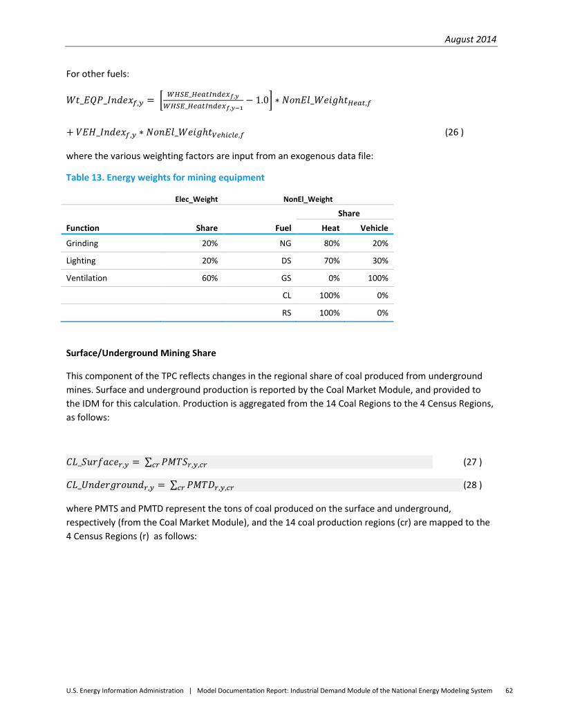
August 2014


For other fuels:

𝑊𝑡_𝐸𝑄𝑃_𝐼𝑛𝑑𝑒𝑥𝑓,𝑦 = � 𝑊𝐻𝑆𝐸_𝐻𝑒𝑎𝑡𝐼𝑛𝑑𝑒𝑥𝑓,𝑦

𝑊𝐻𝑆𝐸_𝐻𝑒𝑎𝑡𝐼𝑛𝑑𝑒𝑥𝑓,𝑦−1− 1.0� ∗ 𝑁𝑜𝑛𝐸𝑙_𝑊𝑒𝑖𝑔ℎ𝑡𝐻𝑒𝑎𝑡,𝑓

+ 𝑉𝐸𝐻_𝐼𝑛𝑑𝑒𝑥𝑓,𝑦 ∗ 𝑁𝑜𝑛𝐸𝑙_𝑊𝑒𝑖𝑔ℎ𝑡𝑉𝑒ℎ𝑖𝑐𝑙𝑒,𝑓 (26 )

where the various weighting factors are input from an exogenous data file:

Table 13. Energy weights for mining equipment

Elec_Weight NonEl_Weight

Function Share Fuel

Share

Heat Vehicle

Grinding 20% NG 80% 20%

Lighting 20% DS 70% 30%

Ventilation 60% GS 0% 100%

CL 100% 0%

RS 100% 0%

Surface/Underground Mining Share

This component of the TPC reflects changes in the regional share of coal produced from underground mines. Surface and underground production is reported by the Coal Market Module, and provided to the IDM for this calculation. Production is aggregated from the 14 Coal Regions to the 4 Census Regions, as follows:

𝐶𝐿_𝑆𝑢𝑟𝑓𝑎𝑐𝑒𝑟,𝑦 = ∑ 𝑃𝑀𝑇𝑆𝑟,𝑦,𝑐𝑟𝑐𝑟 (27 )

𝐶𝐿_𝑈𝑛𝑑𝑒𝑟𝑔𝑟𝑜𝑢𝑛𝑑𝑟,𝑦 = ∑ 𝑃𝑀𝑇𝐷𝑟,𝑦,𝑐𝑟𝑐𝑟 (28 )

where PMTS and PMTD represent the tons of coal produced on the surface and underground, respectively (from the Coal Market Module), and the 14 coal production regions (cr) are mapped to the 4 Census Regions (r) as follows:

August 2014


Table 14. Census region and coal region mapping

Census Region Coal Regions

1 1

2 2,3,6

3 4,5,7

4 8-14

The fraction of annual production from underground mines is then:

𝑈𝑛𝑑𝑒𝑟_𝑆ℎ𝑎𝑟𝑒𝑟,𝑦 = 𝐶𝐿_𝑈𝑛𝑑𝑒𝑟𝑔𝑟𝑜𝑢𝑛𝑑𝑟,𝑦

�𝐶𝐿_𝑈𝑛𝑑𝑒𝑟𝑔𝑟𝑜𝑢𝑛𝑑𝑟,𝑦+𝐶𝐿_𝑆𝑢𝑟𝑓𝑎𝑐𝑒𝑟,𝑦� ( 29 )

and the marginal change in that share is:

𝑈𝑛𝑑𝑒𝑟_𝐼𝑛𝑑𝑒𝑥𝑟,𝑦 = 𝑈𝑛𝑑𝑒𝑟_𝑆ℎ𝑎𝑟𝑒𝑟,𝑦

𝑈𝑛𝑑𝑒𝑟_𝑆ℎ𝑎𝑟𝑒𝑟,𝑦−1− 1.0 ( 30 )

Labor Productivity

Labor productivity is derived from one of the data input files, CLUSER.txt, employed by the Coal Market Module. Each of the production regions has forecasts of productivity by coal type; these are used to construct a production-weighted average productivity forecast, mapped to the Census Regions:

𝐶𝐿_𝐿_𝑃𝑟𝑜𝑑𝑟,𝑦,𝑆𝑢𝑟𝑓 =∑ 𝐵_𝑃𝑟𝑜𝑑𝑟,𝑆𝑢𝑟𝑓,𝑐𝑟∗𝐿_𝑃𝑟𝑜𝑑𝑟,𝑆𝑢𝑟𝑓,𝑐𝑟,∗𝐹𝑅_𝑃𝑟𝑜𝑑𝑟,𝑦,𝑆𝑢𝑟𝑓,𝑐𝑟𝑐𝑟

∑ 𝐵_𝑃𝑟𝑜𝑑𝑟,𝑆𝑢𝑟𝑓,𝑐𝑟,∗𝐿_𝑃𝑟𝑜𝑑𝑟,𝑆𝑢𝑟𝑓,𝑐𝑟𝑐𝑟 ( 31 )

where: B_Prod = Base year (2008) coal production by type and supply region L_Prod = Base year labor productivity in tons/miner/hour FR_Prod = Forecast year labor productivity Surf = Mine type: 1 = Surface, 2 = Underground and the productivity index is:

𝐿_𝑃𝑟𝑜𝑑_𝐼𝑛𝑑𝑒𝑥𝑟,𝑦,𝑆𝑢𝑟𝑓 = 1.0− 𝐶𝐿_𝐿_𝑃𝑟𝑜𝑑𝑟,𝑦,𝑆𝑢𝑟𝑓

𝐶𝐿_𝐿_𝑃𝑟𝑜𝑑𝑟,𝑦−1,𝑆𝑢𝑟𝑓 ( 32 )

TPC calculation The collective TPC by fuel type and region may now be explicitly calculated:

𝑇𝑃𝐶𝑓,𝑦 = 𝑇𝑃𝐶_𝑊𝑒𝑖𝑔ℎ𝑡1,𝑓 ∗ 𝑊𝑡_𝐸𝑄𝑃_𝐼𝑛𝑑𝑒𝑥𝑓,𝑦 + 𝑇𝑃𝐶_𝑊𝑒𝑖𝑔ℎ𝑡2,𝑓 ∗ 𝑈𝑛𝑑𝑒𝑟_𝐼𝑛𝑑𝑒𝑥𝑟,𝑦 + 𝑇𝑃𝐶_𝑊𝑒𝑖𝑔ℎ𝑡3,𝑓 ∗ 𝑈𝑛𝑑𝑒𝑟_𝑆ℎ𝑎𝑟𝑒𝑟,𝑦 ∗ 𝐿_𝑃𝑟𝑜𝑑_𝐼𝑛𝑑𝑒𝑥𝑟,1,𝑦

+ 𝑇𝑃𝐶_𝑊𝑒𝑖𝑔ℎ𝑡3,𝑓 ∗ �1.0 −𝑈𝑛𝑑𝑒𝑟_𝑆ℎ𝑎𝑟𝑒𝑟,𝑦� ∗ 𝐿_𝑃𝑟𝑜𝑑_𝐼𝑛𝑑𝑒𝑥𝑟,2,𝑦 ( 33 )

where the number index represents the weight associated with either the equipment (1), the underground coal production index (2), or the underground coal share (3).

August 2014


The factor weights by region and fuel for mining equipment are as follows, based on analyst judgment:

Table 15. TPC equipment component weights by region

TPC_Weight 1, f Electricity NG Distillate Gasoline Coal Residual Region 1 70% 85% 90% 100% 70% 90% Region 2 70% 85% 90% 100% 70% 90% Region 3 70% 85% 90% 100% 70% 90% Region 4 70% 85% 90% 100% 70% 90%

These may be changed if desired. The weights for the two remaining factors are then calculated:

𝑇𝑃𝐶_𝑊𝑒𝑖𝑔ℎ𝑡2,𝑓 = �1.0−𝑇𝑃𝐶_𝑊𝑒𝑖𝑔ℎ𝑡1,𝑓�2

( 34 )

𝑇𝑃𝐶_𝑊𝑒𝑖𝑔ℎ𝑡3,𝑓 = 1.0 − �𝑇𝑃𝐶_𝑊𝑒𝑖𝑔ℎ𝑡1,𝑓 + 𝑇𝑃𝐶_𝑊𝑒𝑖𝑔ℎ𝑡2,𝑓� ( 35 )

In other words, the difference between 1.0 and the equipment weighting factor is divided between the other two weights.

OGSMTPC The OGSMTPC subroutine calculates the consumption of energy in the oil and gas extraction industry with the major exception of lease and plant fuel, which is natural gas fuel used for any purpose at the lease (extraction) site and fuel used in gas processing plants (lease and plant fuel is modeled in the Natural Gas Transmission and Distribution Model). All other fuels (residual fuel oil, distillate, motor gasoline, electricity, and NGL) are covered by OGSMTPC, as well as that natural gas that is not used in lease and plant fuel, i.e., in natural gas liquid fractionators.

Energy consumption in this sector is largely driven by the number of wells drilled (related to oil and gas volumes) and their productivity.

The amount of fuel (f) demanded by the Oil and Gas Mining industry in year (y) is calculated as follows:

𝑄𝑓,𝑦 = 𝑂𝐺𝑀𝑁𝑦 ∗ 𝑈𝐸𝐶𝑓,𝑦 ( 36 )

where OGMN represents the value of domestic onshore oil and gas production, supplied by the Macroeconomic Activity Module(MAM). The IDM calculates this quantity for each of the four Census Regions. The UEC (by fuel f) changes from year to year (year y-1 to year y) according to the value of the TPC, as follows:

𝑈𝐸𝐶𝑓,𝑦 = 𝑈𝐸𝐶𝑓,𝑦−1 ∗ �1 + 𝑇𝑃𝐶𝑓,𝑦� ( 37 )

August 2014


where the TPC indicates the marginal change in energy intensity from the previous year. The TPC is calculated as the weighted average of three indices representing the marginal change in three factors: vehicle energy intensity, the regional productivity of oil and gas wells, and trends in the share of drilling that results in dry wells. Each of these components is described below.

Factor Indices


As noted in earlier sections, the freight truck model generates fuel economy estimates for three classes of truck. The contribution to the TPC is based on stock-weighted average fuel economy estimates of the truck population and the marginal change in vehicle energy intensity is defined and computed by fuel(f) and year(y) exactly as in AGTPC subroutine on page 48.

Productivity Factors

The Oil & Gas Supply Module (OGSM)33 produces estimates of onshore oil and gas production for 6 production regions (PR), and 7 product types (K), as follows (the variable PROD_Wt is a measure of the relative difficulty of extraction, used in subsequent calculations):

Table 16. Relative difficulty of extraction of oil and gas

K Product Type PROD_Wt

1 Conventional Oil 1.0 2 Enhanced Oil Recovery 3.0 3 Conventional Shallow Gas 1.0 4 Conventional Deep Gas 1.0 5 Tight Gas 3.0 6 Shale Gas 2.0 7 Coal Bed Methane 3.0

Source: OGSM.

The six production regions are displayed in Figure 12:

33 http://www.eia.gov/forecasts/nemsdoc/ogsm/pdf/m063(2013).pdf .

http://www.eia.gov/forecasts/nemsdoc/ogsm/pdf/m063(2013).pdf

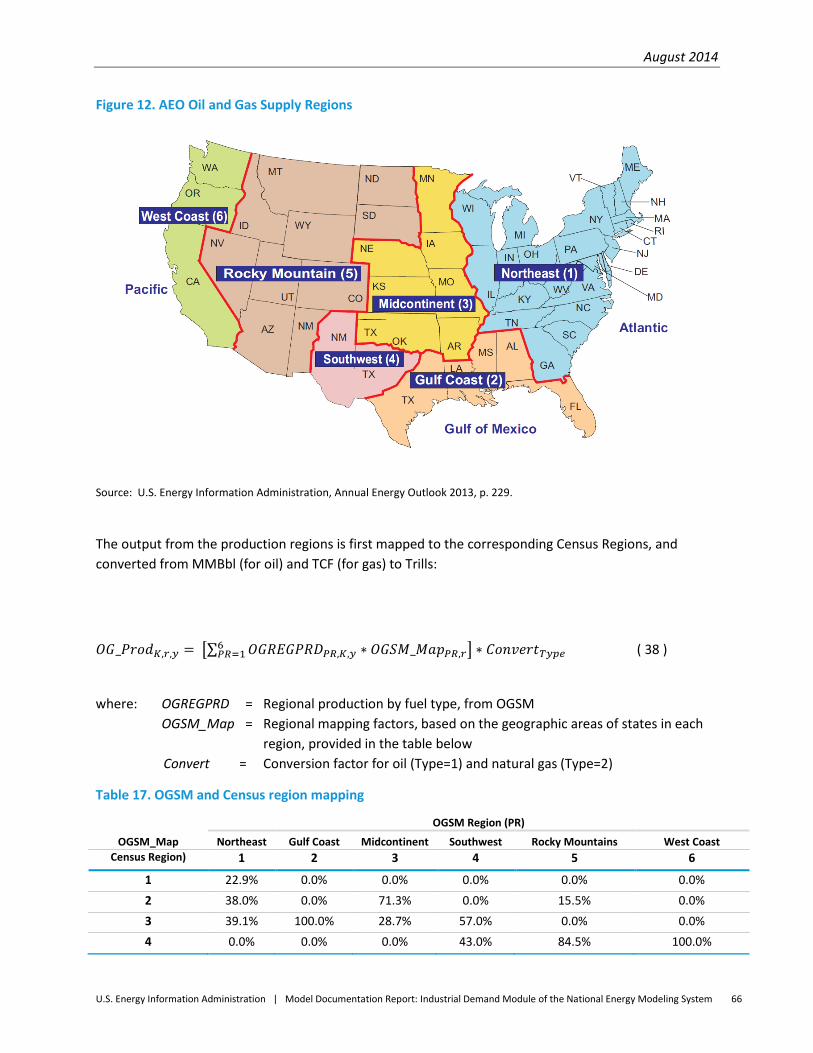
August 2014


Figure 12. AEO Oil and Gas Supply Regions

Source: U.S. Energy Information Administration, Annual Energy Outlook 2013, p. 229.

The output from the production regions is first mapped to the corresponding Census Regions, and converted from MMBbl (for oil) and TCF (for gas) to Trills:

𝑂𝐺_𝑃𝑟𝑜𝑑𝐾,𝑟,𝑦 = �∑ 𝑂𝐺𝑅𝐸𝐺𝑃𝑅𝐷𝑃𝑅,𝐾,𝑦 ∗ 𝑂𝐺𝑆𝑀_𝑀𝑎𝑝𝑃𝑅,𝑟

6𝑃𝑅=1 � ∗ 𝐶𝑜𝑛𝑣𝑒𝑟𝑡𝑇𝑦𝑝𝑒 ( 38 )

where: OGREGPRD = Regional production by fuel type, from OGSM OGSM_Map = Regional mapping factors, based on the geographic areas of states in each

region, provided in the table below Convert = Conversion factor for oil (Type=1) and natural gas (Type=2)

Table 17. OGSM and Census region mapping

OGSM_Map

OGSM Region (PR)

Northeast Gulf Coast Midcontinent Southwest Rocky Mountains West Coast Census Region) 1 2 3 4 5 6

1 22.9% 0.0% 0.0% 0.0% 0.0% 0.0% 2 38.0% 0.0% 71.3% 0.0% 15.5% 0.0% 3 39.1% 100.0% 28.7% 57.0% 0.0% 0.0% 4 0.0% 0.0% 0.0% 43.0% 84.5% 100.0%

August 2014


The share of total production represented by oil is then calculated:

𝑂𝑖𝑙_𝑆ℎ𝑎𝑟𝑒𝑟,𝑦 = ∑ 𝑂𝐺_𝑃𝑟𝑜𝑑𝐾,𝑟,𝑦2𝐾=1

∑ 𝑂𝐺_𝑃𝑟𝑜𝑑𝐾,𝑟,𝑦7𝐾=1

( 39 )

Additionally, the Oil & Gas Production factor, OG_ProdFac, representing the weighted average difficulty of extraction, is calculated as follows:

𝑂𝐺_𝑃𝑟𝑜𝑑𝐹𝑎𝑐𝑇𝑦𝑝𝑒,𝑟,𝑦 = ∑ 𝑂𝐺_𝑃𝑟𝑜𝑑𝐾,𝑟,𝑦∗𝑃𝑅𝑂𝐷_𝑊𝑡𝐾𝐾

∑ 𝑂𝐺_𝑃𝑟𝑜𝑑𝐾,𝑟,𝑦𝐾 ( 40 )

where: K = 1,2 for Oil (1 = conventional oil, 2 = enhanced oil recovery) = 3-7 for Natural Gas (Type = 2) (3 = conventional shallow gas, 4 = conventional deep gas,

5 = tight gas, 6 = shale gas, 7 = coalbed methane) The Productivity Index is then calculated as:

𝑃𝑟𝑜𝑑_𝐼𝑛𝑑𝑒𝑥𝑟,𝑦 = 𝑂𝑖𝑙_𝑆ℎ𝑎𝑟𝑒𝑟,𝑦 ∗ �𝑂𝐺_𝑃𝑟𝑜𝑑𝐹𝑎𝑐𝑇𝑦𝑝𝑒=1,𝑟,𝑦

𝑂𝐺_𝑃𝑟𝑜𝑑𝐹𝑎𝑐𝑇𝑦𝑝𝑒=1,𝑟,𝑦−1− 1.0�

+ �1.0 −𝑂𝑖𝑙_𝑆ℎ𝑎𝑟𝑒𝑟,𝑦� ∗ � 𝑂𝐺_𝑃𝑟𝑜𝑑𝐹𝑎𝑐𝑇𝑦𝑝𝑒=2,𝑟,𝑦

𝑂𝐺_𝑃𝑟𝑜𝑑𝐹𝑎𝑐𝑇𝑦𝑝𝑒=2,𝑟,𝑦−1− 1.0� ( 41 )

Dry Well Index

Another factor affecting the TPC is the share of drilling that produces dry wells. It is assumed that growth in this factor will correlate with increased energy required for overall extraction. The data for successful and dry wells are obtained from the OGSM and are mapped from the six Production Regions (PR) to the four Census Regions (r).

𝑆𝑢𝑐𝑐𝑒𝑠𝑠_𝑊𝑒𝑙𝑙𝐾,𝑟,𝑦 = ∑ 𝑜𝑔𝑠𝑟𝑙48𝑃𝑅,𝐾,𝑦 ∗ 𝑜𝑔𝑤𝑒𝑙𝑙𝑠𝑙48𝑃𝑅,𝐾,𝑦 ∗ 𝑂𝐺𝑆𝑀_𝑀𝑎𝑝𝑃𝑅,𝑟 6𝑃𝑅=1 ( 42 )

𝐷𝑟𝑦_𝑊𝑒𝑙𝑙𝐾,𝑟,𝑦 = ∑ �1.0 − 𝑜𝑔𝑠𝑟𝑙48𝑃𝑅,𝐾,𝑦� ∗ 𝑜𝑔𝑤𝑒𝑙𝑙𝑠𝑙48𝑃𝑅,𝐾,𝑦 ∗ 𝑂𝐺𝑆𝑀_𝑀𝑎𝑝𝑃𝑅,𝑟6𝑃𝑅=1 ( 43 )

𝑇𝑜𝑡𝑎𝑙_𝑊𝑒𝑙𝑙𝐾,𝑟,𝑦 = 𝑆𝑢𝑐𝑐𝑒𝑠𝑠_𝑊𝑒𝑙𝑙𝐾,𝑟,𝑦 + 𝐷𝑟𝑦_𝑊𝑒𝑙𝑙𝐾,𝑟,𝑦 ( 44 )

where: ogsrl48 = Share of successful wells by production region and product type

ogwellsl48 = Total wells drilled, by region and type

OGSM_Map = Regional mapping factors, based on the geographic areas of states in each region, described above.

The production-weighted average dry well percentage by Census Region is then calculated:

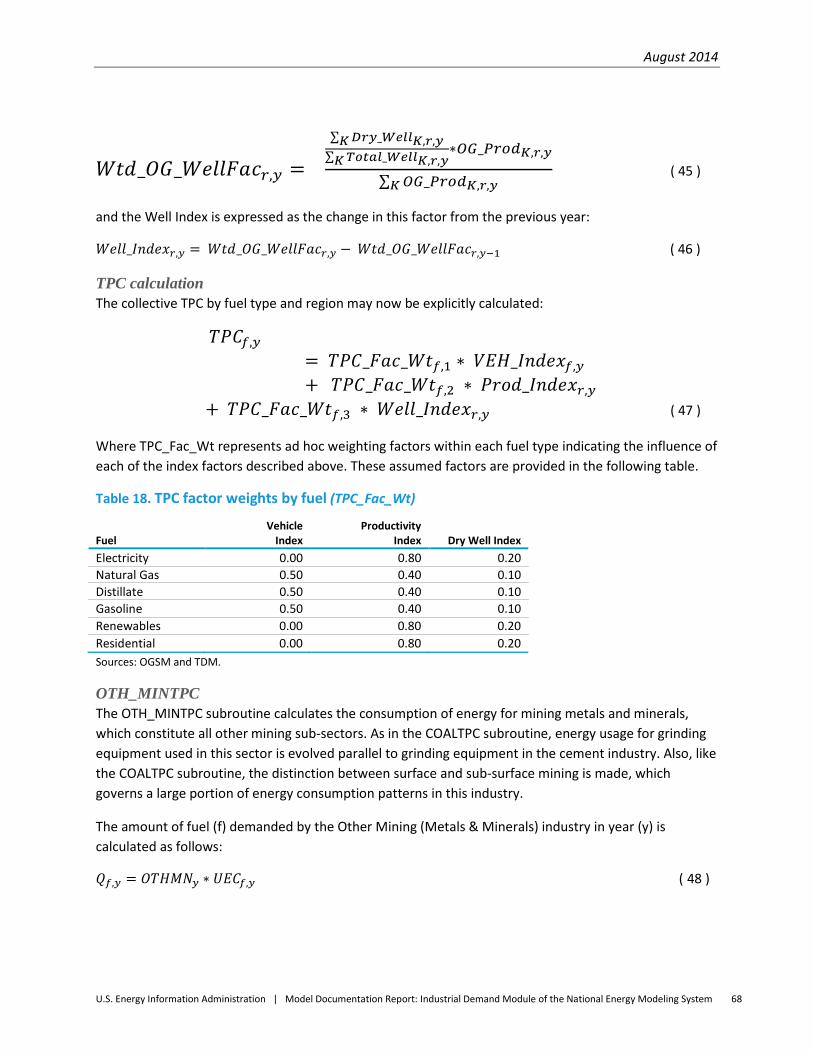
August 2014


𝑊𝑡𝑑_𝑂𝐺_𝑊𝑒𝑙𝑙𝐹𝑎𝑐𝑟,𝑦 = ∑ 𝐷𝑟𝑦_𝑊𝑒𝑙𝑙𝐾,𝑟,𝑦𝐾∑ 𝑇𝑜𝑡𝑎𝑙_𝑊𝑒𝑙𝑙𝐾,𝑟,𝑦𝐾

∗𝑂𝐺_𝑃𝑟𝑜𝑑𝐾,𝑟,𝑦

∑ 𝑂𝐺_𝑃𝑟𝑜𝑑𝐾,𝑟,𝑦𝐾 ( 45 )

and the Well Index is expressed as the change in this factor from the previous year:

𝑊𝑒𝑙𝑙_𝐼𝑛𝑑𝑒𝑥𝑟,𝑦 = 𝑊𝑡𝑑_𝑂𝐺_𝑊𝑒𝑙𝑙𝐹𝑎𝑐𝑟,𝑦 − 𝑊𝑡𝑑_𝑂𝐺_𝑊𝑒𝑙𝑙𝐹𝑎𝑐𝑟,𝑦−1 ( 46 )


𝑇𝑃𝐶𝑓,𝑦= 𝑇𝑃𝐶_𝐹𝑎𝑐_𝑊𝑡𝑓,1 ∗ 𝑉𝐸𝐻_𝐼𝑛𝑑𝑒𝑥𝑓,𝑦 + 𝑇𝑃𝐶_𝐹𝑎𝑐_𝑊𝑡𝑓,2 ∗ 𝑃𝑟𝑜𝑑_𝐼𝑛𝑑𝑒𝑥𝑟,𝑦

+ 𝑇𝑃𝐶_𝐹𝑎𝑐_𝑊𝑡𝑓,3 ∗ 𝑊𝑒𝑙𝑙_𝐼𝑛𝑑𝑒𝑥𝑟,𝑦 ( 47 )

Where TPC_Fac_Wt represents ad hoc weighting factors within each fuel type indicating the influence of each of the index factors described above. These assumed factors are provided in the following table.

Table 18. TPC factor weights by fuel (TPC_Fac_Wt)

Fuel Vehicle

Index Productivity

Index Dry Well Index Electricity 0.00 0.80 0.20 Natural Gas 0.50 0.40 0.10 Distillate 0.50 0.40 0.10 Gasoline 0.50 0.40 0.10 Renewables 0.00 0.80 0.20 Residential 0.00 0.80 0.20 Sources: OGSM and TDM.

OTH_MINTPC The OTH_MINTPC subroutine calculates the consumption of energy for mining metals and minerals, which constitute all other mining sub-sectors. As in the COALTPC subroutine, energy usage for grinding equipment used in this sector is evolved parallel to grinding equipment in the cement industry. Also, like the COALTPC subroutine, the distinction between surface and sub-surface mining is made, which governs a large portion of energy consumption patterns in this industry.

The amount of fuel (f) demanded by the Other Mining (Metals & Minerals) industry in year (y) is calculated as follows:

𝑄𝑓,𝑦 = 𝑂𝑇𝐻𝑀𝑁𝑦 ∗ 𝑈𝐸𝐶𝑓,𝑦 ( 48 )

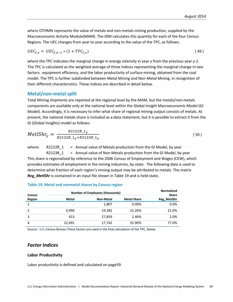
August 2014


where OTHMN represents the value of metals and non-metals mining production, supplied by the Macroeconomic Activity Module(MAM). The IDM calculates this quantity for each of the four Census Regions. The UEC changes from year to year according to the value of the TPC, as follows:

𝑈𝐸𝐶𝑓,𝑦 = 𝑈𝐸𝐶𝑓,𝑦−1 ∗ (1 + 𝑇𝑃𝐶𝑓,𝑦) ( 49 )

where the TPC indicates the marginal change in energy intensity in year y from the previous year y-1. The TPC is calculated as the weighted average of three indices representing the marginal change in two factors: equipment efficiency, and the labor productivity of surface mining, obtained from the coal model. The TPC is further subdivided between Metal Mining and Non-Metal Mining, in recognition of their different characteristics. These indices are described in detail below.

Metal/non-metal split Total Mining shipments are reported at the regional level by the MAM, but the metals/non-metals components are available only at the national level within the Global Insight Macroeconomic Model (GI Model). Accordingly, it is necessary to infer what share of regional mining output consists of metals. At present, the national metals share is included as a data statement, but it is possible to extract it from the GI (Global Insights) model as follows:

𝑀𝑒𝑡𝑙𝑆ℎ𝑟𝑦 = 𝑅2122𝑅_1𝑦𝑅2122𝑅_1𝑦+𝑅2123𝑅_1𝑦

( 50 )

where: R2122R_1 = Annual value of Metals production from the GI Model, by year R2123R_1 = Annual value of Non-Metals production from the GI Model, by year This share is regionalized by reference to the 2006 Census of Employment and Wages (CEW), which provides estimates of employment in the mining industries, by state. The following data is used to determine what fraction of each region’s mining output may be attributed to metals. The matrix Reg_MetlShr is contained in an input file shown in Table 19 and is held static.

Table 19. Metal and nonmetal shares by Census region

Census Region

Number of Employees (thousands) Normalized Share

Reg_MetlShr Metal Non-Metal Metal Share 1 - 1,807 0.00% 0.0%

2 3,490 19,382 15.26% 21.0%

3 413 27,859 1.46% 2.0%

4 22,491 17,742 55.90% 77.0%

Source: U.S. Census Bureau These factors are used in the final calculation of the TPC, below.

Factor Indices

Labor Productivity

Labor productivity is defined and calculated on page59.

August 2014


Equipment

The weighted equipment index is defined and calculated on page 49.

Grinding Equipment

From the results of the cement submodule, the average efficiency of raw grinding equipment per year, or 𝑅𝑎𝑤_𝐺𝑟𝑖𝑛𝑑_𝐸𝑓𝑓𝑦 is extracted to use as a proxy for changes in the energy intensity of mining equipment. This calculation is made on page 61.


The freight truck model generates fuel economy estimates for three classes of truck. The contribution to the TPC is based on stock-weighted average fuel economy estimates of the truck population, and the marginal change in vehicle energy intensity is defined and computed by fuel(f) and year(y) exactly as in AGTPC subroutine on page 48.

The weighted equipment index is then calculated for Metals and Non-Metals separately.

For Electricity (Metals Mining):

𝑊𝑡_𝑀𝑒𝑡_𝐸𝑄𝑃_𝐼𝑛𝑑𝑒𝑥𝑓,𝑦 = �𝑅𝑎𝑤_𝐺𝑟𝑖𝑛𝑑_𝐸𝑓𝑓𝑦𝑅𝑎𝑤_𝐺𝑟𝑖𝑛𝑑_𝐸𝑓𝑓𝑦−1

− 1.0� ∗ 𝐸𝑙𝑒𝑐_𝑀𝑒𝑡_𝑊𝑒𝑖𝑔ℎ𝑡𝐺𝑟𝑖𝑛𝑑

+ �𝑊𝐻𝑆𝐸_𝐿𝑖𝑔ℎ𝑡𝐼𝑛𝑑𝑒𝑥𝑟,𝑦

𝑊𝐻𝑆𝐸_𝐿𝑖𝑔ℎ𝑡𝐼𝑛𝑑𝑒𝑥𝑟,𝑦−1− 1.0� ∗ 𝐸𝑙𝑒𝑐_𝑀𝑒𝑡_𝑊𝑒𝑖𝑔ℎ𝑡𝐿𝑖𝑔ℎ𝑡

+ � 𝑊𝐻𝑆𝐸_𝑉𝑒𝑛𝑡𝐼𝑛𝑑𝑒𝑥𝑟,𝑦

𝑊𝐻𝑆𝐸_𝑉𝑒𝑛𝑡𝐼𝑛𝑑𝑒𝑥𝑟,𝑦−1− 1.0� ∗ 𝐸𝑙𝑒𝑐_𝑀𝑒𝑡_𝑊𝑒𝑖𝑔ℎ𝑡𝑉𝑒𝑛𝑡 ( 51 )

Similarly, for Non-Metals:

𝑊𝑡_𝑁𝑀_𝐸𝑄𝑃_𝐼𝑛𝑑𝑒𝑥𝑓,𝑦 = �𝑅𝑎𝑤_𝐺𝑟𝑖𝑛𝑑_𝐸𝑓𝑓𝑦𝑅𝑎𝑤_𝐺𝑟𝑖𝑛𝑑_𝐸𝑓𝑓𝑦−1

− 1.0� ∗ 𝐸𝑙𝑒𝑐_𝑁𝑀_𝑊𝑒𝑖𝑔ℎ𝑡𝐺𝑟𝑖𝑛𝑑

+ �𝑊𝐻𝑆𝐸_𝐿𝑖𝑔ℎ𝑡𝐼𝑛𝑑𝑒𝑥𝑟,𝑦

𝑊𝐻𝑆𝐸_𝐿𝑖𝑔ℎ𝑡𝐼𝑛𝑑𝑒𝑥𝑟,𝑦−1− 1.0� ∗ 𝐸𝑙𝑒𝑐_𝑁𝑀_𝑊𝑒𝑖𝑔ℎ𝑡_𝐿𝑖𝑔ℎ𝑡

+ � 𝑊𝐻𝑆𝐸_𝑉𝑒𝑛𝑡𝐼𝑛𝑑𝑒𝑥𝑟,𝑦

𝑊𝐻𝑆𝐸_𝑉𝑒𝑛𝑡𝐼𝑛𝑑𝑒𝑥𝑟,𝑦−1− 1.0� ∗ 𝐸𝑙𝑒𝑐_𝑁𝑀_𝑊𝑒𝑖𝑔ℎ𝑡𝑉𝑒𝑛𝑡 ( 52 )

Where the difference in the calculation is in the relative weights ascribed to Grinding, Lighting, and Pumping (through its proxy, ventilation). These factors are as follows:

August 2014


Table 20. Electric equipment weights

Variable Grinding Lighting Pumping

Metals Elec_Met_Wt 0.20 0.20 0.60

Non-Metals Elec_NM_Wt 0.60 0.20 0.20

Sources: CDM (for Lighting and Pumping), IDM Cement submodule (for Grinding).

For Other Fuels (Metals):

𝑊𝑡_𝑀𝑒𝑡_𝐸𝑄𝑃_𝐼𝑛𝑑𝑒𝑥𝑓,𝑦 = �𝑊𝐻𝑆𝐸_𝐻𝑒𝑎𝑡𝐼𝑛𝑑𝑒𝑥𝑓,𝑟,𝑦

𝑊𝐻𝑆𝐸_𝐻𝑒𝑎𝑡𝐼𝑛𝑑𝑒𝑥𝑓,𝑟,𝑦−1− 1.0� ∗ 𝑁𝑜𝑛𝐸𝑙_𝑀𝑒𝑡_𝑊𝑒𝑖𝑔ℎ𝑡𝐻𝑒𝑎𝑡,𝑓

+ 𝑉𝐸𝐻_𝐼𝑛𝑑𝑒𝑥𝑓,𝑦 ∗ 𝑁𝑜𝑛𝐸𝑙_𝑀𝑒𝑡_𝑊𝑒𝑖𝑔ℎ𝑡𝑉𝑒ℎ𝑖𝑐𝑙𝑒,𝑓 ( 53 )

and Non-Metals:

𝑊𝑡_𝑁𝑀_𝐸𝑄𝑃_𝐼𝑛𝑑𝑒𝑥𝑓,𝑦 = �𝑊𝐻𝑆𝐸_𝐻𝑒𝑎𝑡𝐼𝑛𝑑𝑒𝑥𝑓,𝑟,𝑦

𝑊𝐻𝑆𝐸_𝐻𝑒𝑎𝑡𝐼𝑛𝑑𝑒𝑥𝑓,𝑟,𝑦−1− 1.0� ∗ 𝑁𝑜𝑛𝐸𝑙_𝑁𝑀_𝑊𝑒𝑖𝑔ℎ𝑡𝐻𝑒𝑎𝑡,𝑓

+ 𝑉𝐸𝐻_𝐼𝑛𝑑𝑒𝑥𝑓,𝑦 ∗ 𝑁𝑜𝑛𝐸𝑙_𝑁𝑀_𝑊𝑒𝑖𝑔ℎ𝑡𝑉𝑒ℎ𝑖𝑐𝑙𝑒,𝑓 ( 54 )

where the current weighting factors for Metals and Non-Metals are identical. The model assigns the same weights to the two variables in order to make subsequent, user-specified changes easier to implement.

Table 21. Non-electric equipment weights (Metals and non-metals)

TPC_Met_Wt r,1,f & TPC_NM_Wt r,1,f NG Distillate Gasoline Coal Residual

Heating 80% 70% 0% 100% 100% Vehicles 20% 30% 100% 0% 0%

Source: CDM and TDM.


𝑇𝑃𝐶𝑟,𝑓,𝑦 = �𝑇𝑃𝐶_𝑀𝑒𝑡_𝑊𝑡r,1,f ∗ 𝑊𝑡_𝑀𝑒𝑡_𝐸𝑄𝑃_𝐼𝑛𝑑𝑒𝑥𝑟,𝑦

+ 𝑇𝑃𝐶_𝑀𝑒𝑡_𝑊𝑡r,2,f ∗ 𝐿_𝑃𝑟𝑜𝑑_𝐼𝑛𝑑𝑒𝑥𝑟,𝑦

� ∗ 𝑀𝑒𝑡𝑙𝑆ℎ𝑟𝑦 ∗ 𝑅𝑒𝑔_𝑀𝑒𝑡𝑙𝑆ℎ𝑟𝑟

+ �𝑇𝑃𝐶_𝑁𝑀_𝑊𝑡𝑟,1,𝑓 ∗ 𝑊𝑡_𝑁𝑀_𝐸𝑄𝑃_𝐼𝑛𝑑𝑒𝑥𝑟,𝑦

+ 𝑇𝑃𝐶_𝑁𝑀_𝑊𝑡𝑟,2,𝑓 ∗ 𝐿_𝑃𝑟𝑜𝑑_𝐼𝑛𝑑𝑒𝑥𝑟,𝑦

� ∗ �1.0 −𝑀𝑒𝑡𝑙𝑆ℎ𝑟𝑦 ∗ 𝑅𝑒𝑔_𝑀𝑒𝑡𝑙𝑆ℎ𝑟𝑟� ( 55 )

August 2014


where the TPC Equipment Index weights for both Metals and Non-Metals are provided in the following table, based on analyst judgment:

Table 22. TPC equipment component weights by region

TPC_Met_Wt r,1,f & TPC_NM_Wt r,1,f Metal & Non-Metal Electricity NG Distillate Gasoline Coal Residual Region 1 70 85% 90% 100% 90% 90%

Region 2 70 85% 90% 100% 90% 90%

Region 3 70 85% 90% 100% 90% 90%

Region 4 70 85% 90% 100% 90% 90%

The Non-Equipment (i.e., Labor Productivity) Index weights are then calculated:

𝑇𝑃𝐶_𝑀𝑒𝑡_𝑊𝑡𝑟,1,𝑓 = 1.0 − 𝑇𝑃𝐶_𝑀𝑒𝑡_𝑊𝑡𝑟,1,𝑓 ( 56 )

As with the Non-Electric equipment weights, above, the factors are identical across regions and for Metals/Non-Metals mining. This explicit separation of the two mine types in the code provides an easily adaptable structure for testing and scenario development.

GLASS _INDUSTRY Submodule Glass is an inorganic product that is typically produced by melting a mixture of silica (sand, 75%), soda (around 15%), and a calcium compound (usually lime, 10%). To this are added the desired metallic oxides that serve as coloring agents. All industrial glass is manufactured by:

1. Preparing the right mix of raw materials. 2. Melting and refining the raw materials. 3. Forming and finishing the molten glass into desired products.

The mix of raw materials depends on the type of glass being manufactured and its desired properties and color. Melting varies in scale, temperature, and residence time, and is typically carried out in tank melters. Forming is much more diverse considering the wide range of products from the glass industry. Some glass products require additional finishing processes.

Products manufactured by the U.S. glass industry span a broad diversity, including food and beverage containers, flat glass, fiberglass insulation, windows for automobiles and buildings, video displays, cookware, leaded crystal, and light bulbs. In the glass submodule these products are classified under four general categories - flat glass, container glass, blown glass, and fiberglass (wool insulation and textile fiber). Blown glass (also known as specialty glass) is the smallest of the four glass industry segments. The large diversity of products is accompanied by an equally large diversity of forming processes. Table 22 shows the four categories of glass (by NAICS code) that are modeled.

August 2014


Table 23. Major U.S. glass industry segments and typical products

Type of Glass NAICS code Description

Flat Glass 327211 Sheet plate and float glass for residential and

commercial construction, automotive applications,

tabletops, and mirrors.

Container Glass 327213 Packaging of foods, beverages, household chemicals,

cosmetics, and pharmaceuticals.

Blown Glass 327212 Pressed and blown glass for tableware, cookware,

lighting, televisions, liquid crystal displays, laboratory

equipment, and optical communications.

Fiberglass 327993 Fiberglass (glass wool) insulation for buildings, roofing,

and panels.

327212 Textile and plastic reinforcement fibers for the

construction, transportation, and marine industries.

Figure 13 summarizes the glass submodule execution. The code is run for each year in the projection period. The glass industry shipments in dollars are determined by the MAM. These shipments are then assigned to the four glass segments (subroutine Glass Segment Shipping). The capacity requirement is estimated in metric tons for each glass segment. The capacity estimates include yearly estimates of both the remaining baseline capacity before the projection years and remaining new capacity added during the projection years, as well as the additional capacity required each year to meet demand. Flat glass and Blown glass include finishing processes. All four glass segments have forming, furnace, and preparation processes. As new capacity is added for each process step in each glass segment, the technology is selected based on an evaluation of the relative economic benefit of the available technologies. An adjustment is made to fuel consumption for oxy-fuel furnaces (subroutine OxyFuel). The results are then reported.

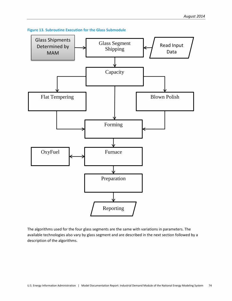
August 2014


Figure 13. Subroutine Execution for the Glass Submodule

The algorithms used for the four glass segments are the same with variations in parameters. The available technologies also vary by glass segment and are described in the next section followed by a description of the algorithms.

Glass Shipments Determined by

MAM

Glass Segment Shipping

Read Input Data

Reporting

Capacity

Flat Tempering Blown Polish

Forming

Furnace

Preparation

OxyFuel

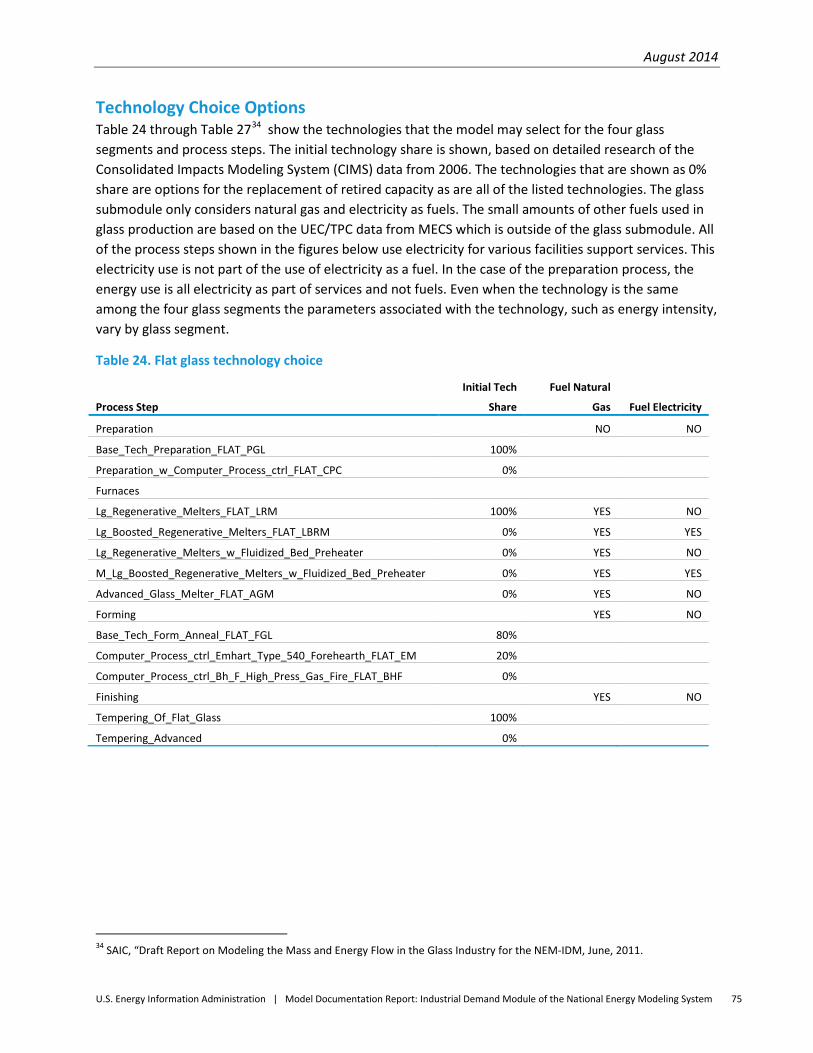
August 2014


Technology Choice Options Table 24 through Table 2734 show the technologies that the model may select for the four glass segments and process steps. The initial technology share is shown, based on detailed research of the Consolidated Impacts Modeling System (CIMS) data from 2006. The technologies that are shown as 0% share are options for the replacement of retired capacity as are all of the listed technologies. The glass submodule only considers natural gas and electricity as fuels. The small amounts of other fuels used in glass production are based on the UEC/TPC data from MECS which is outside of the glass submodule. All of the process steps shown in the figures below use electricity for various facilities support services. This electricity use is not part of the use of electricity as a fuel. In the case of the preparation process, the energy use is all electricity as part of services and not fuels. Even when the technology is the same among the four glass segments the parameters associated with the technology, such as energy intensity, vary by glass segment.

Table 24. Flat glass technology choice

Process Step

Initial Tech

Share

Fuel Natural

Gas Fuel Electricity

Preparation NO NO

Base_Tech_Preparation_FLAT_PGL 100%

Preparation_w_Computer_Process_ctrl_FLAT_CPC 0%

Furnaces

Lg_Regenerative_Melters_FLAT_LRM 100% YES NO

Lg_Boosted_Regenerative_Melters_FLAT_LBRM 0% YES YES

Lg_Regenerative_Melters_w_Fluidized_Bed_Preheater 0% YES NO

M_Lg_Boosted_Regenerative_Melters_w_Fluidized_Bed_Preheater 0% YES YES

Advanced_Glass_Melter_FLAT_AGM 0% YES NO

Forming YES NO

Base_Tech_Form_Anneal_FLAT_FGL 80%

Computer_Process_ctrl_Emhart_Type_540_Forehearth_FLAT_EM 20%

Computer_Process_ctrl_Bh_F_High_Press_Gas_Fire_FLAT_BHF 0%

Finishing YES NO

Tempering_Of_Flat_Glass 100%

Tempering_Advanced 0%

34 SAIC, “Draft Report on Modeling the Mass and Energy Flow in the Glass Industry for the NEM-IDM, June, 2011.

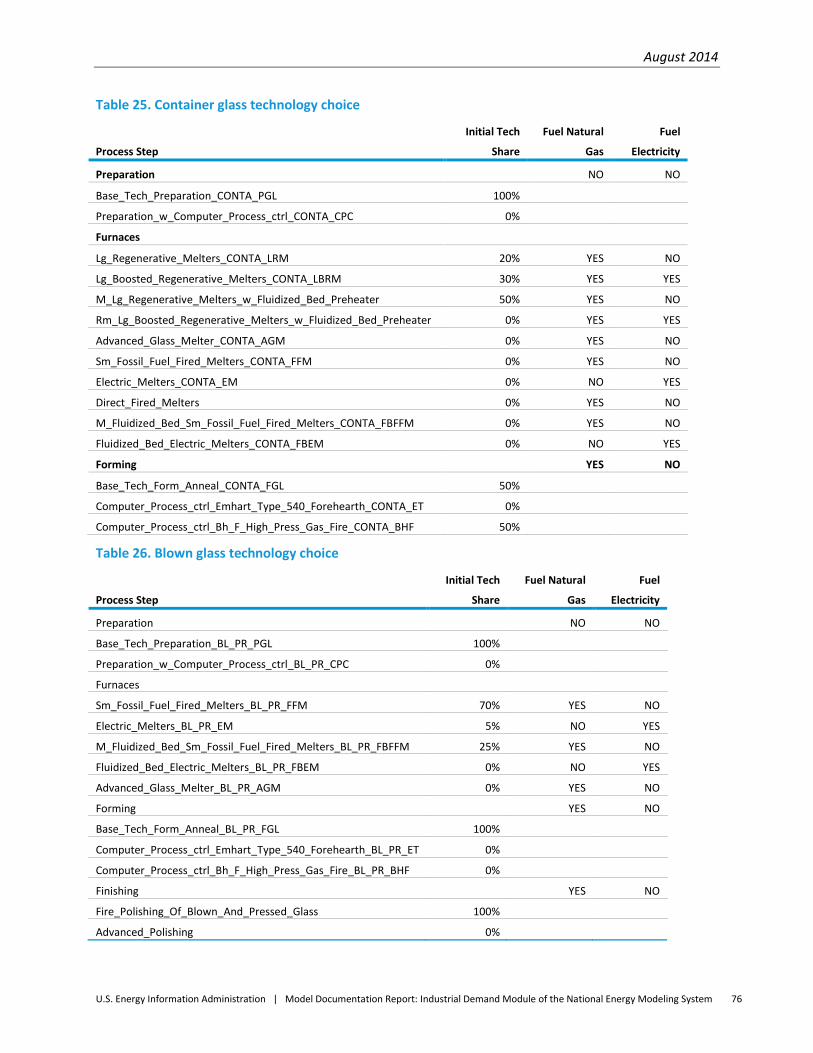
August 2014


Table 25. Container glass technology choice

Process Step

Initial Tech

Share

Fuel Natural

Gas

Fuel

Electricity

Preparation NO NO

Base_Tech_Preparation_CONTA_PGL 100%

Preparation_w_Computer_Process_ctrl_CONTA_CPC 0%

Furnaces

Lg_Regenerative_Melters_CONTA_LRM 20% YES NO

Lg_Boosted_Regenerative_Melters_CONTA_LBRM 30% YES YES

M_Lg_Regenerative_Melters_w_Fluidized_Bed_Preheater 50% YES NO

Rm_Lg_Boosted_Regenerative_Melters_w_Fluidized_Bed_Preheater 0% YES YES

Advanced_Glass_Melter_CONTA_AGM 0% YES NO

Sm_Fossil_Fuel_Fired_Melters_CONTA_FFM 0% YES NO

Electric_Melters_CONTA_EM 0% NO YES

Direct_Fired_Melters 0% YES NO

M_Fluidized_Bed_Sm_Fossil_Fuel_Fired_Melters_CONTA_FBFFM 0% YES NO

Fluidized_Bed_Electric_Melters_CONTA_FBEM 0% NO YES

Forming YES NO

Base_Tech_Form_Anneal_CONTA_FGL 50%

Computer_Process_ctrl_Emhart_Type_540_Forehearth_CONTA_ET 0%

Computer_Process_ctrl_Bh_F_High_Press_Gas_Fire_CONTA_BHF 50%

Table 26. Blown glass technology choice

Process Step

Initial Tech

Share

Fuel Natural

Gas

Fuel

Electricity

Preparation NO NO

Base_Tech_Preparation_BL_PR_PGL 100%

Preparation_w_Computer_Process_ctrl_BL_PR_CPC 0%

Furnaces

Sm_Fossil_Fuel_Fired_Melters_BL_PR_FFM 70% YES NO

Electric_Melters_BL_PR_EM 5% NO YES

M_Fluidized_Bed_Sm_Fossil_Fuel_Fired_Melters_BL_PR_FBFFM 25% YES NO

Fluidized_Bed_Electric_Melters_BL_PR_FBEM 0% NO YES

Advanced_Glass_Melter_BL_PR_AGM 0% YES NO

Forming YES NO

Base_Tech_Form_Anneal_BL_PR_FGL 100%

Computer_Process_ctrl_Emhart_Type_540_Forehearth_BL_PR_ET 0%

Computer_Process_ctrl_Bh_F_High_Press_Gas_Fire_BL_PR_BHF 0%

Finishing YES NO

Fire_Polishing_Of_Blown_And_Pressed_Glass 100%

Advanced_Polishing 0%

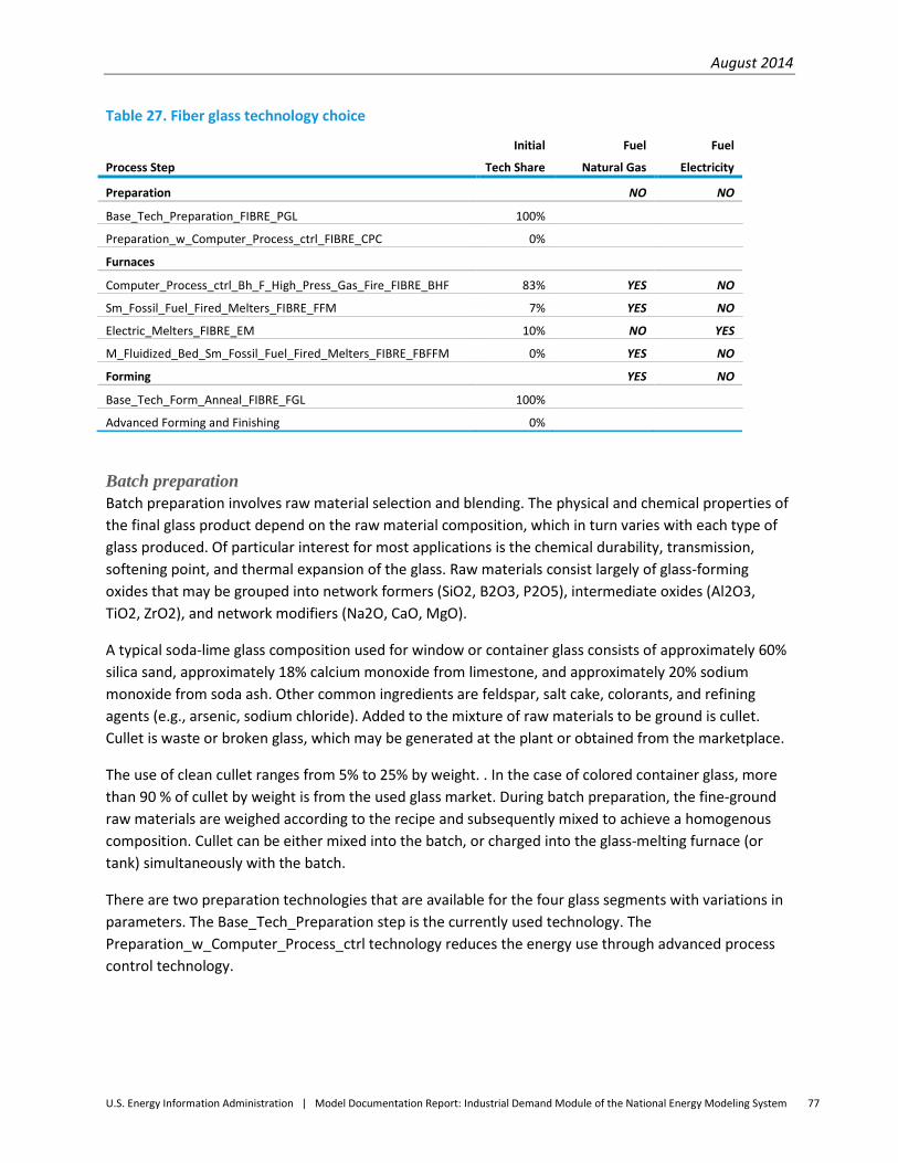
August 2014


Table 27. Fiber glass technology choice

Process Step

Initial

Tech Share

Fuel

Natural Gas

Fuel

Electricity

Preparation NO NO

Base_Tech_Preparation_FIBRE_PGL 100%

Preparation_w_Computer_Process_ctrl_FIBRE_CPC 0%

Furnaces

Computer_Process_ctrl_Bh_F_High_Press_Gas_Fire_FIBRE_BHF 83% YES NO

Sm_Fossil_Fuel_Fired_Melters_FIBRE_FFM 7% YES NO

Electric_Melters_FIBRE_EM 10% NO YES

M_Fluidized_Bed_Sm_Fossil_Fuel_Fired_Melters_FIBRE_FBFFM 0% YES NO

Forming YES NO

Base_Tech_Form_Anneal_FIBRE_FGL 100%

Advanced Forming and Finishing 0%

Batch preparation Batch preparation involves raw material selection and blending. The physical and chemical properties of the final glass product depend on the raw material composition, which in turn varies with each type of glass produced. Of particular interest for most applications is the chemical durability, transmission, softening point, and thermal expansion of the glass. Raw materials consist largely of glass-forming oxides that may be grouped into network formers (SiO2, B2O3, P2O5), intermediate oxides (Al2O3, TiO2, ZrO2), and network modifiers (Na2O, CaO, MgO).

A typical soda-lime glass composition used for window or container glass consists of approximately 60% silica sand, approximately 18% calcium monoxide from limestone, and approximately 20% sodium monoxide from soda ash. Other common ingredients are feldspar, salt cake, colorants, and refining agents (e.g., arsenic, sodium chloride). Added to the mixture of raw materials to be ground is cullet. Cullet is waste or broken glass, which may be generated at the plant or obtained from the marketplace.

The use of clean cullet ranges from 5% to 25% by weight. . In the case of colored container glass, more than 90 % of cullet by weight is from the used glass market. During batch preparation, the fine-ground raw materials are weighed according to the recipe and subsequently mixed to achieve a homogenous composition. Cullet can be either mixed into the batch, or charged into the glass-melting furnace (or tank) simultaneously with the batch.

There are two preparation technologies that are available for the four glass segments with variations in parameters. The Base_Tech_Preparation step is the currently used technology. The Preparation_w_Computer_Process_ctrl technology reduces the energy use through advanced process control technology.

August 2014


Melting furnaces The melting of glass, with the exception of a few blown glass manufacturing processes, is accomplished with continuously operating tank furnaces. Discontinuous glass melting processes operate as pot furnaces and day tanks. In pot furnaces, one or more refractory crucibles are filled with batch and cullet and placed in a gas-fired or electrically heated furnace. After melting the batch, the temperature of the furnace is typically increased to lower the melt viscosity and activate refining agents to remove bubbles from the melt (refining) and then lowered to condition the glass for forming. Day-tanks are small tanks that are charged with batch and cullet. As in a pot furnace, the temperatures are adjusted for melting, refining and conditioning of the glass melt.

A typical glass-melting tank consists of a batch charging area (the doghouse) attached to a refractory basin covered by a refractory superstructure (the crown). Presently, most glass furnaces in the U.S. are heated with natural gas. Common heating methods are air-fuel burners and, more recently, oxy-fuel burners. Some furnaces use direct electrical heating (Joule heating), in particular, for wool-type fiberglass production that provide more uniform temperature distributions compared with gas heaters. Combinations of both heating methods (electric boosting) is used to help melt the glass since glass is an electrical conductor at high temperatures. Electric boosting typically consists of 10-30% of the total energy demand, but increases production rates and the flexibility of the furnace operation.

Common to both flat and container industry segments are regenerative and recuperative furnaces. Fiberglass furnaces are generally smaller than container and flat glass furnaces. Pressed and blown glass (specialty glass) furnaces are the smallest. To improve energy efficiency and achieve higher flame temperatures, air-fuel furnaces typically recover heat from exhaust gas streams with regenerative systems to preheat the combustion air. In regenerative systems, the exhaust gases stream through large chambers packed with refractory bricks arranged in patterns forming open conduits.35 A fluidized bed reactor is a type of reactor device that can be used to carry out a variety of multiphase chemical reactions where a fluid (gas or liquid) is passed through a granular solid material at high enough velocities to suspend the solid and cause it to behave as though it were a fluid. The Advanced Glass Melter is a projected technology based on the most energy-efficient current technologies.

Forming and conditioning After completion of the refining stage, the homogenous, bubble-free glass leaves the tank and enters the forehearth, sometimes through a specifically designed pathway (channel or throat). The main function of the forehearth is to condition the glass, i.e. to deliver glass with the desired temperature and temperature distribution to the forming process. Any deviations from the desired thermal profile can cause undesirable differences in viscosity and subsequently lead to visible defects in the finished product. Forehearths can be gas-fired or electrically heated.

The conditioned glass is delivered from the forehearth to the forming equipment at a constant rate. Depending on the process, the viscous glass stream is either continuously shaped (float glass, fiberglass),

35 Worrell, Ernst, Christina Galitsky, et al., March 2008, Energy Efficiency Improvement and Cost Savings Opportunities for the Glass Industry, An Energy Star Guide for Energy and Plant Managers, Ernest Orlando Lawrence Berkeley National Laboratory, LBNL-57335.

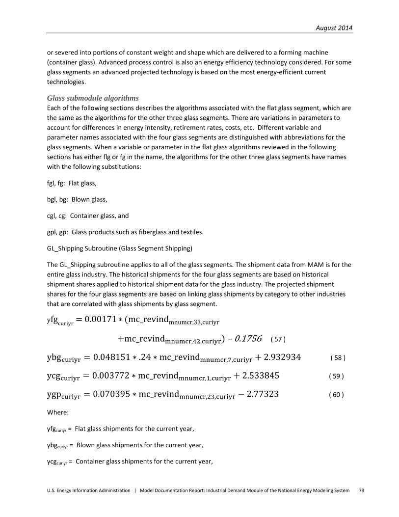
August 2014


or severed into portions of constant weight and shape which are delivered to a forming machine (container glass). Advanced process control is also an energy efficiency technology considered. For some glass segments an advanced projected technology is based on the most energy-efficient current technologies.

Glass submodule algorithms Each of the following sections describes the algorithms associated with the flat glass segment, which are the same as the algorithms for the other three glass segments. There are variations in parameters to account for differences in energy intensity, retirement rates, costs, etc. Different variable and parameter names associated with the four glass segments are distinguished with abbreviations for the glass segments. When a variable or parameter in the flat glass algorithms reviewed in the following sections has either flg or fg in the name, the algorithms for the other three glass segments have names with the following substitutions:

fgl, fg: Flat glass,

bgl, bg: Blown glass,

cgl, cg: Container glass, and

gpl, gp: Glass products such as fiberglass and textiles.

GL_Shipping Subroutine (Glass Segment Shipping)

The GL_Shipping subroutine applies to all of the glass segments. The shipment data from MAM is for the entire glass industry. The historical shipments for the four glass segments are based on historical shipment shares applied to historical shipment data for the glass industry. The projected shipment shares for the four glass segments are based on linking glass shipments by category to other industries that are correlated with glass shipments by glass segment.

yfgcuriyr = 0.00171 ∗ (mc_revindmnumcr,33,curiyr

+mc_revindmnumcr,42,curiyr) – 0.1756 ( 57 )

ybgcuriyr = 0.048151 ∗ .24 ∗ mc_revindmnumcr,7,curiyr + 2.932934 ( 58 )

ycgcuriyr = 0.003772 ∗ mc_revindmnumcr,1,curiyr + 2.533845 ( 59 )

ygpcuriyr = 0.070395 ∗ mc_revindmnumcr,23,curiyr − 2.77323 ( 60 )

Where:

yfgcuriyr = Flat glass shipments for the current year,

ybgcuriyr = Blown glass shipments for the current year,

ycgcuriyr = Container glass shipments for the current year,

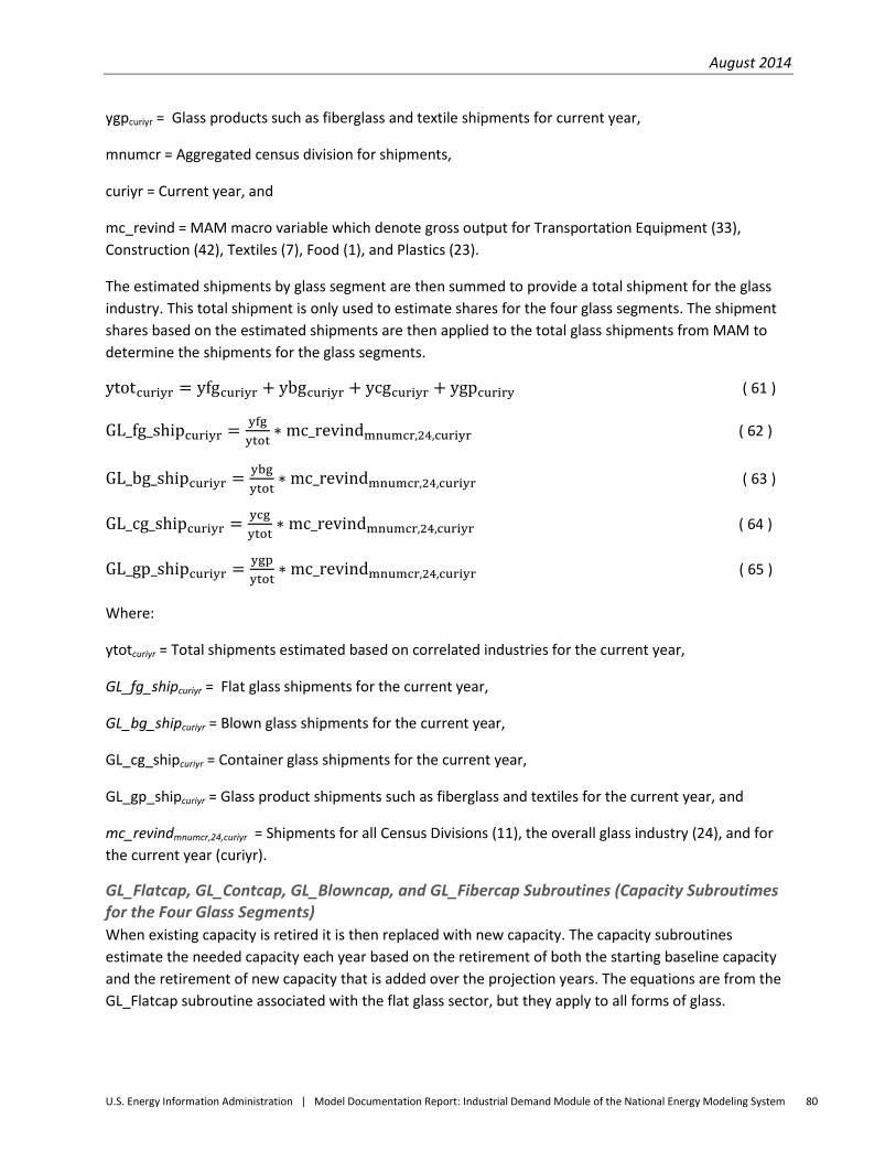
August 2014


ygpcuriyr = Glass products such as fiberglass and textile shipments for current year,

mnumcr = Aggregated census division for shipments,

curiyr = Current year, and

mc_revind = MAM macro variable which denote gross output for Transportation Equipment (33), Construction (42), Textiles (7), Food (1), and Plastics (23).

The estimated shipments by glass segment are then summed to provide a total shipment for the glass industry. This total shipment is only used to estimate shares for the four glass segments. The shipment shares based on the estimated shipments are then applied to the total glass shipments from MAM to determine the shipments for the glass segments.

ytotcuriyr = yfgcuriyr + ybgcuriyr + ycgcuriyr + ygpcuriry ( 61 )

GL_fg_shipcuriyr = yfgytot

∗ mc_revindmnumcr,24,curiyr ( 62 )

GL_bg_shipcuriyr = ybgytot


GL_cg_shipcuriyr = ycgytot


GL_gp_shipcuriyr = ygpytot


Where:

ytotcuriyr = Total shipments estimated based on correlated industries for the current year,

GL_fg_shipcuriyr = Flat glass shipments for the current year,

GL_bg_shipcuriyr = Blown glass shipments for the current year,

GL_cg_shipcuriyr = Container glass shipments for the current year,

GL_gp_shipcuriyr = Glass product shipments such as fiberglass and textiles for the current year, and

mc_revindmnumcr,24,curiyr = Shipments for all Census Divisions (11), the overall glass industry (24), and for the current year (curiyr).

GL_Flatcap, GL_Contcap, GL_Blowncap, and GL_Fibercap Subroutines (Capacity Subroutimes for the Four Glass Segments) When existing capacity is retired it is then replaced with new capacity. The capacity subroutines estimate the needed capacity each year based on the retirement of both the starting baseline capacity and the retirement of new capacity that is added over the projection years. The equations are from the GL_Flatcap subroutine associated with the flat glass sector, but they apply to all forms of glass.

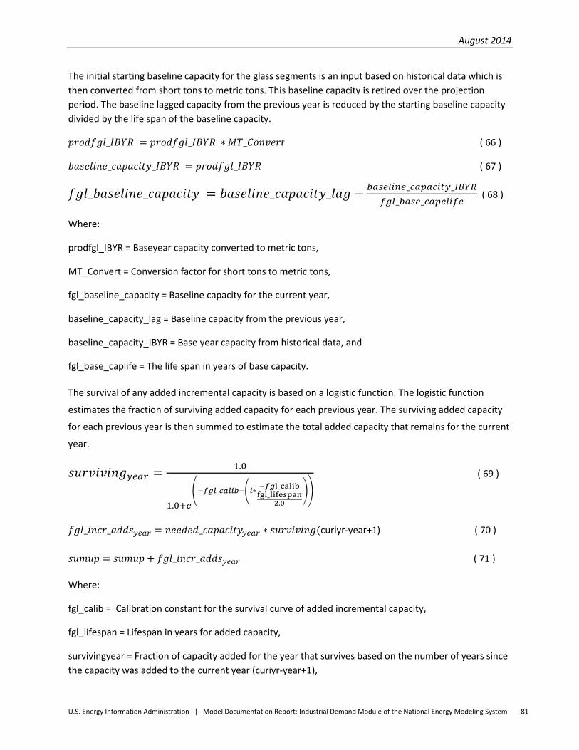
August 2014


The initial starting baseline capacity for the glass segments is an input based on historical data which is then converted from short tons to metric tons. This baseline capacity is retired over the projection period. The baseline lagged capacity from the previous year is reduced by the starting baseline capacity divided by the life span of the baseline capacity.

𝑝𝑟𝑜𝑑𝑓𝑔𝑙_𝐼𝐵𝑌𝑅 = 𝑝𝑟𝑜𝑑𝑓𝑔𝑙_𝐼𝐵𝑌𝑅 ∗ 𝑀𝑇_𝐶𝑜𝑛𝑣𝑒𝑟𝑡 ( 66 )

𝑏𝑎𝑠𝑒𝑙𝑖𝑛𝑒_𝑐𝑎𝑝𝑎𝑐𝑖𝑡𝑦_𝐼𝐵𝑌𝑅 = 𝑝𝑟𝑜𝑑𝑓𝑔𝑙_𝐼𝐵𝑌𝑅 ( 67 )

𝑓𝑔𝑙_𝑏𝑎𝑠𝑒𝑙𝑖𝑛𝑒_𝑐𝑎𝑝𝑎𝑐𝑖𝑡𝑦 = 𝑏𝑎𝑠𝑒𝑙𝑖𝑛𝑒_𝑐𝑎𝑝𝑎𝑐𝑖𝑡𝑦_𝑙𝑎𝑔 − 𝑏𝑎𝑠𝑒𝑙𝑖𝑛𝑒_𝑐𝑎𝑝𝑎𝑐𝑖𝑡𝑦_𝐼𝐵𝑌𝑅𝑓𝑔𝑙_𝑏𝑎𝑠𝑒_𝑐𝑎𝑝𝑒𝑙𝑖𝑓𝑒

( 68 )

Where:

prodfgl_IBYR = Baseyear capacity converted to metric tons,

MT_Convert = Conversion factor for short tons to metric tons,

fgl_baseline_capacity = Baseline capacity for the current year,

baseline_capacity_lag = Baseline capacity from the previous year,

baseline_capacity_IBYR = Base year capacity from historical data, and

fgl_base_caplife = The life span in years of base capacity.

The survival of any added incremental capacity is based on a logistic function. The logistic function

estimates the fraction of surviving added capacity for each previous year. The surviving added capacity

for each previous year is then summed to estimate the total added capacity that remains for the current

year.

𝑠𝑢𝑟𝑣𝑖𝑣𝑖𝑛𝑔𝑦𝑒𝑎𝑟 = 1.0

1.0+𝑒�−𝑓𝑔𝑙_𝑐𝑎𝑙𝑖𝑏−�𝑖∗ −𝑓𝑔l_calibfgl_lifespan

2.0��

( 69 )

𝑓𝑔𝑙_𝑖𝑛𝑐𝑟_𝑎𝑑𝑑𝑠𝑦𝑒𝑎𝑟 = 𝑛𝑒𝑒𝑑𝑒𝑑_𝑐𝑎𝑝𝑎𝑐𝑖𝑡𝑦𝑦𝑒𝑎𝑟 ∗ 𝑠𝑢𝑟𝑣𝑖𝑣𝑖𝑛𝑔(curiyr-year+1) ( 70 )

𝑠𝑢𝑚𝑢𝑝 = 𝑠𝑢𝑚𝑢𝑝 + 𝑓𝑔𝑙_𝑖𝑛𝑐𝑟_𝑎𝑑𝑑𝑠𝑦𝑒𝑎𝑟 ( 71 )

Where:

fgl_calib = Calibration constant for the survival curve of added incremental capacity,

fgl_lifespan = Lifespan in years for added capacity,

survivingyear = Fraction of capacity added for the year that survives based on the number of years since the capacity was added to the current year (curiyr-year+1),

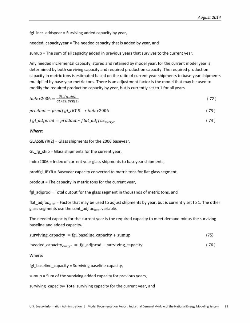
August 2014


fgl_incr_addsyear = Surviving added capacity by year,

needed_capacityyear = The needed capacity that is added by year, and

sumup = The sum of all capacity added in previous years that survives to the current year.

Any needed incremental capacity, stored and retained by model year, for the current model year is determined by both surviving capacity and required production capacity. The required production capacity in metric tons is estimated based on the ratio of current year shipments to base-year shipments multiplied by base-year metric tons. There is an adjustment factor is the model that may be used to modify the required production capacity by year, but is currently set to 1 for all years.

𝑖𝑛𝑑𝑒𝑥2006 = 𝐺𝐿_𝑓𝑔_𝑠ℎ𝑖𝑝𝐺𝐿𝐴𝑆𝑆𝐼𝐵𝑌𝑅(2)

( 72 )

𝑝𝑟𝑜𝑑𝑜𝑢𝑡 = 𝑝𝑟𝑜𝑑𝑓𝑔𝑙_𝐼𝐵𝑌𝑅 ∗ 𝑖𝑛𝑑𝑒𝑥2006 ( 73 )

𝑓𝑔𝑙_𝑎𝑑𝑗𝑝𝑟𝑜𝑑 = 𝑝𝑟𝑜𝑑𝑜𝑢𝑡 ∗ 𝑓𝑙𝑎𝑡_𝑎𝑑𝑗𝑓𝑎𝑐𝑐𝑢𝑟𝑖𝑦𝑟 ( 74 )

Where:

GLASSIBYR(2) = Glass shipments for the 2006 baseyear,

GL_fg_ship = Glass shipments for the current year,

index2006 = Index of current year glass shipments to baseyear shipments,

prodfgl_IBYR = Baseyear capacity converted to metric tons for flat glass segment,

prodout = The capacity in metric tons for the current year,

fgl_adjprod = Total output for the glass segment in thousands of metric tons, and

flat_adjfaccuriyr = Factor that may be used to adjust shipments by year, but is currently set to 1. The other glass segments use the cont_adjfaccuriyr variable.

The needed capacity for the current year is the required capacity to meet demand minus the surviving baseline and added capacity.

surviving_capacity = fgl_baseline_capacity + sumup (75)

needed_capacitycuriyr = fgl_adjprod− surviving_capacity ( 76 )

Where:

fgl_baseline_capacity = Surviving baseline capacity,

sumup = Sum of the surviving added capacity for previous years,

surviving_capacity= Total surviving capacity for the current year, and

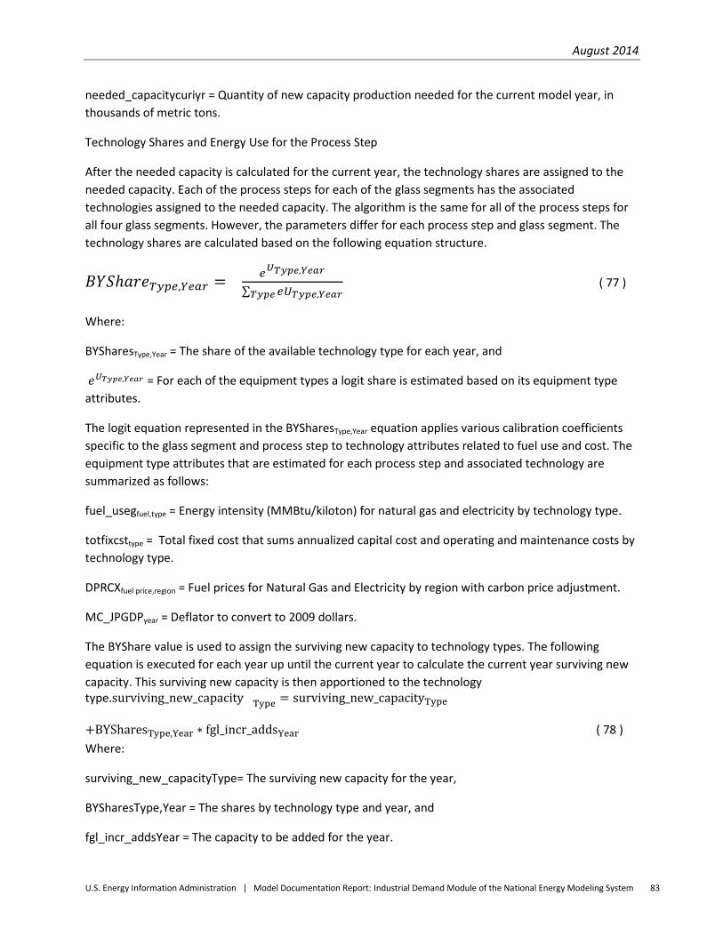
August 2014


needed_capacitycuriyr = Quantity of new capacity production needed for the current model year, in thousands of metric tons.

Technology Shares and Energy Use for the Process Step

After the needed capacity is calculated for the current year, the technology shares are assigned to the needed capacity. Each of the process steps for each of the glass segments has the associated technologies assigned to the needed capacity. The algorithm is the same for all of the process steps for all four glass segments. However, the parameters differ for each process step and glass segment. The technology shares are calculated based on the following equation structure.

𝐵𝑌𝑆ℎ𝑎𝑟𝑒𝑇𝑦𝑝𝑒,𝑌𝑒𝑎𝑟 = 𝑒𝑈𝑇𝑦𝑝𝑒,𝑌𝑒𝑎𝑟

∑ 𝑒𝑈𝑇𝑦𝑝𝑒,𝑌𝑒𝑎𝑟𝑇𝑦𝑝𝑒 ( 77 )

Where:

BYSharesType,Year = The share of the available technology type for each year, and

𝑒𝑈𝑇𝑦𝑝𝑒,𝑌𝑒𝑎𝑟 = For each of the equipment types a logit share is estimated based on its equipment type attributes.

The logit equation represented in the BYSharesType,Year equation applies various calibration coefficients specific to the glass segment and process step to technology attributes related to fuel use and cost. The equipment type attributes that are estimated for each process step and associated technology are summarized as follows:

fuel_usegfuel,type = Energy intensity (MMBtu/kiloton) for natural gas and electricity by technology type.

totfixcsttype = Total fixed cost that sums annualized capital cost and operating and maintenance costs by technology type.

DPRCXfuel price,region = Fuel prices for Natural Gas and Electricity by region with carbon price adjustment.

MC_JPGDPyear = Deflator to convert to 2009 dollars.

The BYShare value is used to assign the surviving new capacity to technology types. The following equation is executed for each year up until the current year to calculate the current year surviving new capacity. This surviving new capacity is then apportioned to the technology type.surviving_new_capacity Type = surviving_new_capacityType

+BYSharesType,Year ∗ fgl_incr_addsYear ( 78 ) Where:

surviving_new_capacityType= The surviving new capacity for the year,

BYSharesType,Year = The shares by technology type and year, and

fgl_incr_addsYear = The capacity to be added for the year.

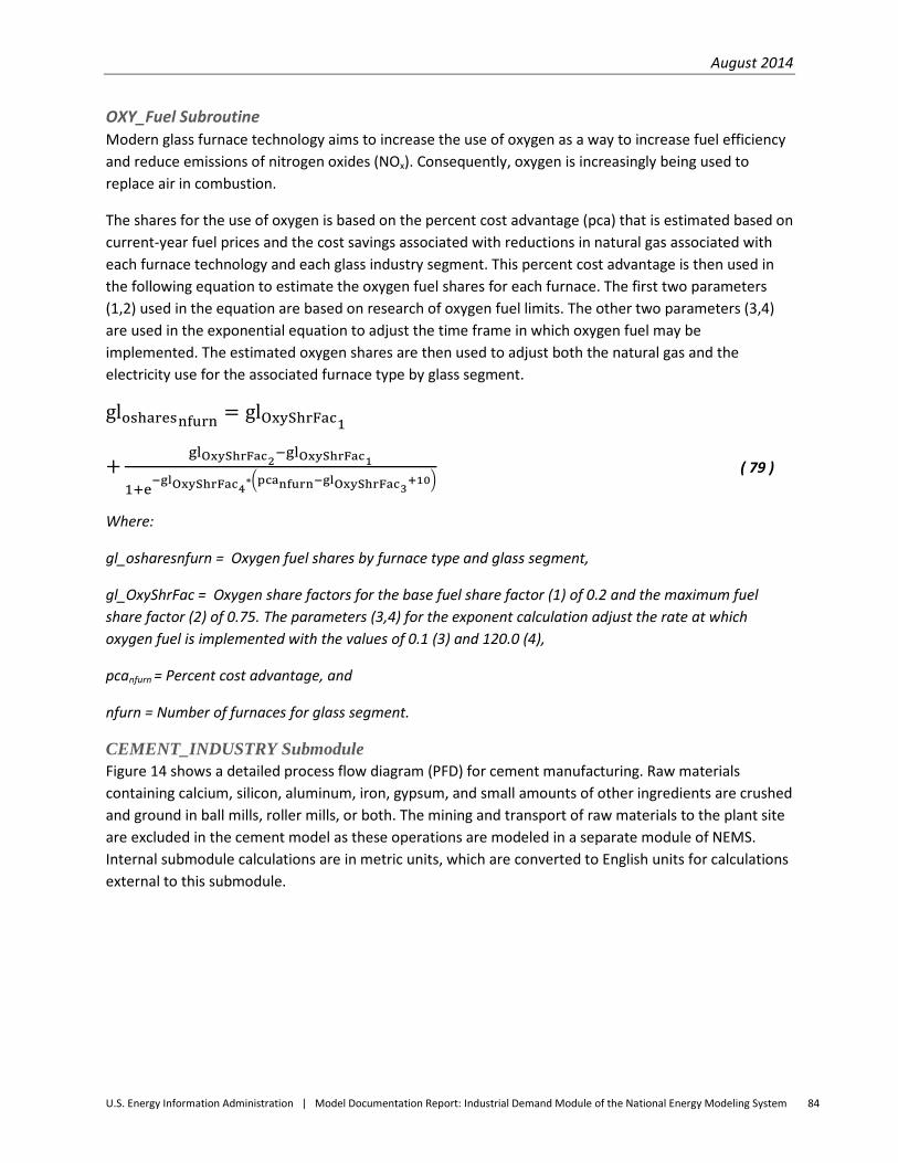
August 2014


OXY_Fuel Subroutine Modern glass furnace technology aims to increase the use of oxygen as a way to increase fuel efficiency and reduce emissions of nitrogen oxides (NOx). Consequently, oxygen is increasingly being used to replace air in combustion.

The shares for the use of oxygen is based on the percent cost advantage (pca) that is estimated based on current-year fuel prices and the cost savings associated with reductions in natural gas associated with each furnace technology and each glass industry segment. This percent cost advantage is then used in the following equation to estimate the oxygen fuel shares for each furnace. The first two parameters (1,2) used in the equation are based on research of oxygen fuel limits. The other two parameters (3,4) are used in the exponential equation to adjust the time frame in which oxygen fuel may be implemented. The estimated oxygen shares are then used to adjust both the natural gas and the electricity use for the associated furnace type by glass segment.

glosharesnfurn = glOxyShrFac1

+glOxyShrFac2−glOxyShrFac1

1+e−glOxyShrFac4

∗�pcanfurn−glOxyShrFac3+10�

( 79 )

Where:

gl_osharesnfurn = Oxygen fuel shares by furnace type and glass segment,

gl_OxyShrFac = Oxygen share factors for the base fuel share factor (1) of 0.2 and the maximum fuel share factor (2) of 0.75. The parameters (3,4) for the exponent calculation adjust the rate at which oxygen fuel is implemented with the values of 0.1 (3) and 120.0 (4),

pcanfurn = Percent cost advantage, and

nfurn = Number of furnaces for glass segment.

CEMENT_INDUSTRY Submodule Figure 14 shows a detailed process flow diagram (PFD) for cement manufacturing. Raw materials containing calcium, silicon, aluminum, iron, gypsum, and small amounts of other ingredients are crushed and ground in ball mills, roller mills, or both. The mining and transport of raw materials to the plant site are excluded in the cement model as these operations are modeled in a separate module of NEMS. Internal submodule calculations are in metric units, which are converted to English units for calculations external to this submodule.

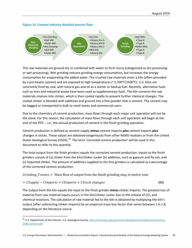
August 2014


Figure 14. Cement industry detailed process flow

The raw materials are ground dry or combined with water to form slurry (categorized as dry processing or wet processing). Wet grinding reduces grinding energy consumption, but increases the energy consumption for evaporating the added water. The crushed raw materials enter a kiln (often preceded by a pre-heater system) and are exposed to high temperatures (~2,700°F/1500oC). U.S. kilns are commonly fired by coal, with natural gas and oil as a starter or backup fuel. Recently, alternative fuels such as tires and industrial waste have been used as supplementary fuels. The kiln converts the raw materials mixture into clinker, which is then cooled rapidly to prevent further chemical changes. The cooled clinker is blended with additives and ground into a fine powder that is cement. The cement may be bagged or transported in bulk to retail stores and commercial users.

Due to the chemistry of cement production, mass flows through each major unit operation will not be the same. For this reason, the calculation of mass flows through each unit operation will begin at the end of the PFD -- i.e., the annual production of cement in the finish grinding operation.

Cement production is defined as cement supply minus cement imports plus cement exports plus changes in stocks. These values are obtained exogenously from other NEMS modules or from the United States Geological Survey (USGS).36 The term ‘corrected cement production’ will be used in this document to refer to this quantity.

The total output from the finish grinders equals the corrected cement production. Inputs to the finish grinders consist of (a) clinker from the kiln/clinker cooler (b) additives, such as gypsum and fly ash, and (c) imported clinker. The amount of additives supplied to the fine grinders is calculated as a percentage of the corrected cement production.

𝐺𝑟𝑖𝑛𝑑𝑖𝑛𝑔_𝑇𝑜𝑛𝑛𝑒𝑠 = Mass flow of output from the finish grinding step, in metric tons

= 𝐶𝑆𝑢𝑝𝑝𝑙𝑦 − 𝐶𝐼𝑚𝑝𝑜𝑟𝑡𝑠 + 𝐶𝐸𝑥𝑝𝑜𝑟𝑡𝑠 + 𝐶𝑆𝑡𝑜𝑐𝑘 𝑐ℎ𝑎𝑛𝑔𝑒𝑠 (80)

The output from the kiln equals the input to the finish grinder minus clinker imports. The greatest loss of material from raw material inputs occurs in the kiln/clinker cooler due to the release of CO2 and chemical reactions. The calculation of raw material fed to the kiln is obtained by multiplying the kiln’s output (after subtracting clinker imports) by an empirical mass-loss factor that varies between 1.6-1.8, depending on the literature source.

36 U.S. Department of the Interior, U.S. Geological Survey, http://minerals.usgs.gov/minerals/pubs/commodity/cement/mcs-2006-cement.pdf.

•Dry Grinding •Ball Mill •Roller Mill

•Wet Grinding •Ball Mill •Roller Mill

Raw Materials Grinding

•Dry Kiln •Rotary Kiln A •Rotary Kiln B •Rotary Kiln C

•Wet Kiln •Rotary Kiln

Kiln Operations

•Ball Mills •Type A •Type B

•Roller Mills •Type A •Type B

Finish Grinding

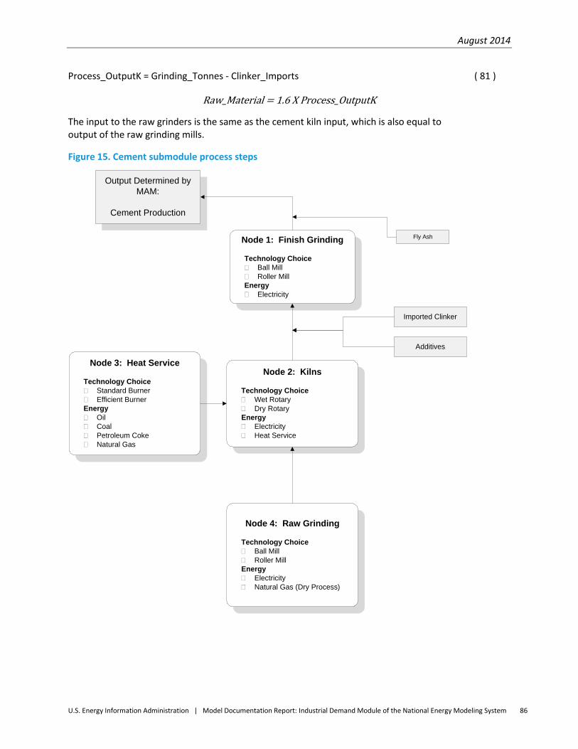
http://minerals.usgs.gov/minerals/pubs/commodity/cement/mcs-2006-cement.pdf

http://minerals.usgs.gov/minerals/pubs/commodity/cement/mcs-2006-cement.pdf

August 2014


Process_OutputK = Grinding_Tonnes - Clinker_Imports ( 81 )

Raw_Material = 1.6 X Process_OutputK

The input to the raw grinders is the same as the cement kiln input, which is also equal to output of the raw grinding mills.

Figure 15. Cement submodule process steps

Output Determined by MAM:

Cement Production

Node 1: Finish Grinding

Technology Choice� Ball Mill� Roller MillEnergy� Electricity

Node 2: Kilns

Technology Choice� Wet Rotary� Dry RotaryEnergy� Electricity� Heat Service

Imported Clinker

Additives

Fly Ash

Node 3: Heat Service

Technology Choice� Standard Burner� Efficient BurnerEnergy� Oil� Coal� Petroleum Coke� Natural Gas

Node 4: Raw Grinding

Technology Choice� Ball Mill� Roller MillEnergy� Electricity� Natural Gas (Dry Process)

August 2014


FINISH_GRIND_CAP (Node 1) The FINISH_GRIND_CAP subroutine represents cement production capacity requirements for IDM.

The output of the Finish Grinding node is the total quantity of cement shipments (in thousand metric tons) in a given year.

𝑆ℎ𝑖𝑝𝑚𝑒𝑛𝑡𝑠 = Shipments_IBYR2 ∗ � 𝑂𝑈𝑇𝐼𝑁𝐷22,11𝐶𝐸𝑀𝐸𝑁𝑇𝐼𝐵𝑌𝑅

� ( 82 )

where

𝑆ℎ𝑖𝑝𝑚𝑒𝑛𝑡𝑠 = Physical quantity of cement shipments, in thousands of metric tons, projected for the cement industry

𝑆ℎ𝑖𝑝𝑚𝑒𝑛𝑡𝑠_𝐼𝐵𝑌𝑅2 = Physical quantity of cement shipments, in thousands of metric tons in 2006, as reported by the U.S. Geological Survey

𝑂𝑈𝑇𝐼𝑁𝐷22,11 = Gross value of output for the cement industry (IDM industry code of 22) for the nation in the current projection year, as determined by NEMS MAM, and

𝐶𝐸𝑀𝐸𝑁𝑇𝐼𝐵𝑌𝑅 = Gross value of output for the cement industry for the nation in year 2010, as determined by MAM.

The output requirements of the finish grinders are reduced by the inclusion of certain additives, such as fly-ash, following the grinding step:

𝐺𝑟𝑖𝑛𝑑𝑖𝑛𝑔_𝑇𝑜𝑛𝑛𝑒𝑠 = 𝑆ℎ𝑖𝑝𝑚𝑒𝑛𝑡𝑠 ∗ (1.0− 𝐹𝑙𝑦𝐴𝑠ℎ ) ( 83 )

where:

𝐺𝑟𝑖𝑛𝑑𝑖𝑛𝑔_𝑇𝑜𝑛𝑛𝑒𝑠 = Quantity of output from the finish grinding step, in thousands of metric

tons

𝐹𝑙𝑦𝐴𝑠ℎ = Percentage of additives, which is currently held constant at 5.0%.

Cement production in 2008 represents existing baseline capacity, which is allocated among the four competing types of finish grinders as follows:

𝐵𝑎𝑠𝑒𝐶𝑎𝑝𝐹𝑇𝑦𝑝𝑒 = 𝐺𝑟𝑖𝑛𝑑𝑖𝑛𝑔_𝑇𝑜𝑛𝑛𝑒𝑠 ∗ 𝑇𝑒𝑐ℎ_𝑆ℎ𝑎𝑟𝑒𝑇𝑦𝑝𝑒 ( 84 )

where: 𝐵𝑎𝑠𝑒𝐶𝑎𝑝𝐹𝑇𝑦𝑝𝑒 = Initial baseline capacity, by equipment type


tons, and 𝑇𝑒𝑐ℎ_𝑆ℎ𝑎𝑟𝑒𝑇𝑦𝑝𝑒 = Initial allocation of finish grinding capacity, based on CIMS data, for 2008.

For each year following the base year (i.e., 2008), incremental additions to Finish Grinding capacity are based on the following assumptions:

• Baseline capacity is retired at a linear rate over a fixed time frame (initially set to 20 years)

August 2014


• Production demand in excess of surviving baseline capacity will be met with replacement equipment, and

• Equipment acquired after 2008 will retire according to a logistic function.

Baseline capacity that survives is computed as follows:

𝐵𝑎𝑠𝑒𝐶𝑎𝑝𝐹𝑇𝑦𝑝𝑒 = 𝐵𝑎𝑠𝑒𝐶𝑎𝑝_𝐿𝑎𝑔𝑇𝑦𝑝𝑒 – �𝐵𝑎𝑠𝑒𝐶𝑎𝑝_𝐼𝐵𝑌𝑅𝑇𝑦𝑝𝑒𝐵𝑎𝑠𝑒𝐿𝑖𝑓𝑒𝑐

� ( 85 )

where:

𝐵𝑎𝑠𝑒𝐶𝑎𝑝𝐹𝑇𝑦𝑝𝑒 = Surviving baseline capacity, by equipment type,

𝐵𝑎𝑠𝑒𝐶𝑎𝑝_𝐿𝑎𝑔𝑇𝑦𝑝𝑒 = Lagged surviving baseline capacity, by equipment type,

𝐵𝑎𝑠𝑒𝐶𝑎𝑝_𝐼𝐵𝑌𝑅𝑇𝑦𝑝𝑒 = Baseline capacity in year 2008, by equipment type, and

𝐵𝑎𝑠𝑒𝐿𝑖𝑓𝑒𝑐 = Assumed lifetime of baseline capacity.

The survival of any added incremental capacity is based on a logistic function. This function is written as:

𝑁𝑒𝑤_𝐶𝑎𝑝_𝑆𝑢𝑟𝑣𝐹𝑖+1 = 1

1+exp�− 𝐶𝑎𝑙𝑖𝑏𝑟𝑎𝑡𝑖𝑜𝑛𝑐 ∗ �1.0− � 2.0∗(𝑖)𝐿𝑖𝑓𝑒𝑆𝑝𝑎𝑛𝑐��

( 86 )

where

𝑁𝑒𝑤_𝐶𝑎𝑝_𝑆𝑢𝑟𝑣𝐹𝑖+1 = Rate of survival for added incremental capacity,

𝐿𝑖𝑓𝑒𝑆𝑝𝑎𝑛𝑐 = Assumed lifetime of added finish grinding capacity,

𝐶𝑎𝑙𝑖𝑏𝑟𝑎𝑡𝑖𝑜𝑛𝑐 = Calibration constant for the survival curve of added incremental capacity, and

𝑖 = A year index representing the Vintage (i.e., number of years since acquisition of added

capacity.

The survival function determines the share of needed capacity added in a given year that survives to the current model year, as shown in Figure 16

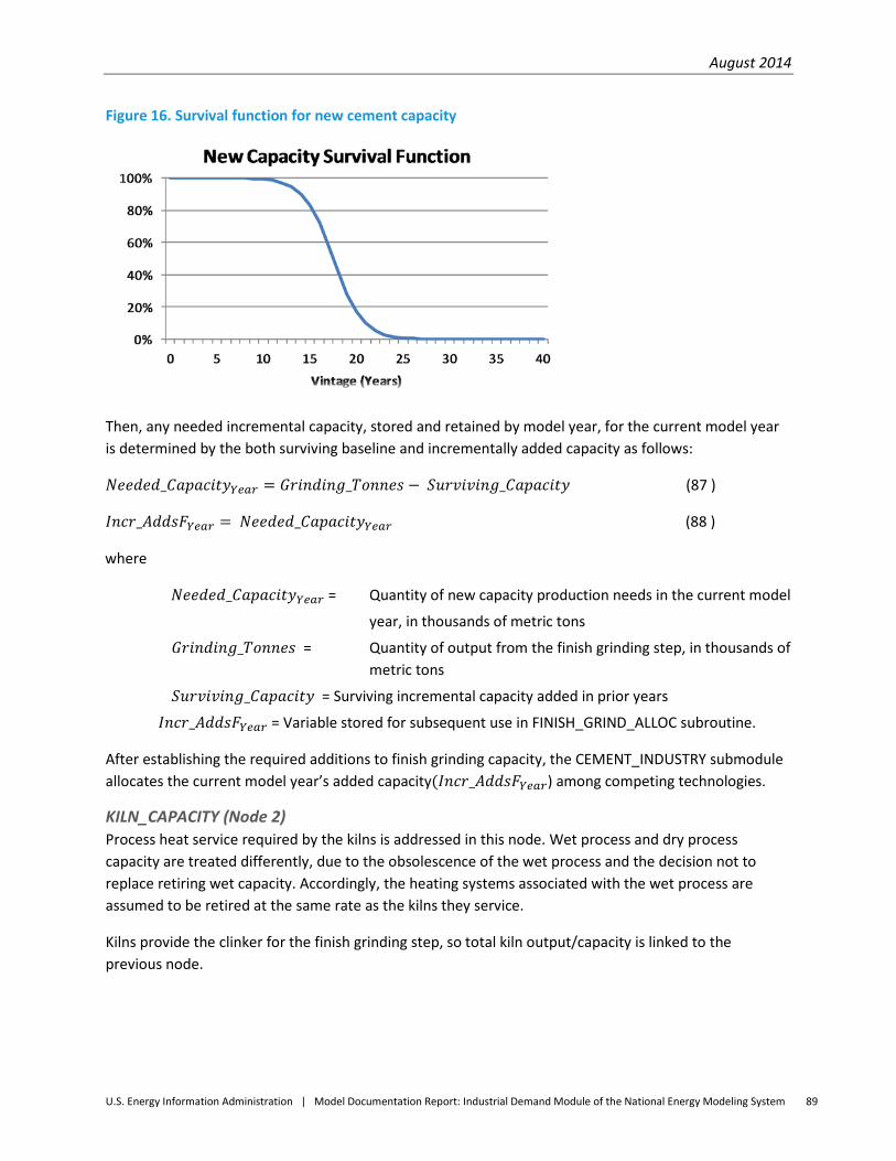
August 2014


Figure 16. Survival function for new cement capacity

Then, any needed incremental capacity, stored and retained by model year, for the current model year is determined by the both surviving baseline and incrementally added capacity as follows:

𝑁𝑒𝑒𝑑𝑒𝑑_𝐶𝑎𝑝𝑎𝑐𝑖𝑡𝑦𝑌𝑒𝑎𝑟 = 𝐺𝑟𝑖𝑛𝑑𝑖𝑛𝑔_𝑇𝑜𝑛𝑛𝑒𝑠 − 𝑆𝑢𝑟𝑣𝑖𝑣𝑖𝑛𝑔_𝐶𝑎𝑝𝑎𝑐𝑖𝑡𝑦 (87 )

𝐼𝑛𝑐𝑟_𝐴𝑑𝑑𝑠𝐹𝑌𝑒𝑎𝑟 = 𝑁𝑒𝑒𝑑𝑒𝑑_𝐶𝑎𝑝𝑎𝑐𝑖𝑡𝑦𝑌𝑒𝑎𝑟 (88 )

where

𝑁𝑒𝑒𝑑𝑒𝑑_𝐶𝑎𝑝𝑎𝑐𝑖𝑡𝑦𝑌𝑒𝑎𝑟 = Quantity of new capacity production needs in the current model

year, in thousands of metric tons

𝐺𝑟𝑖𝑛𝑑𝑖𝑛𝑔_𝑇𝑜𝑛𝑛𝑒𝑠 = Quantity of output from the finish grinding step, in thousands of metric tons

𝑆𝑢𝑟𝑣𝑖𝑣𝑖𝑛𝑔_𝐶𝑎𝑝𝑎𝑐𝑖𝑡𝑦 = Surviving incremental capacity added in prior years

𝐼𝑛𝑐𝑟_𝐴𝑑𝑑𝑠𝐹𝑌𝑒𝑎𝑟 = Variable stored for subsequent use in FINISH_GRIND_ALLOC subroutine.

After establishing the required additions to finish grinding capacity, the CEMENT_INDUSTRY submodule allocates the current model year’s added capacity(𝐼𝑛𝑐𝑟_𝐴𝑑𝑑𝑠𝐹𝑌𝑒𝑎𝑟) among competing technologies.

KILN_CAPACITY (Node 2) Process heat service required by the kilns is addressed in this node. Wet process and dry process capacity are treated differently, due to the obsolescence of the wet process and the decision not to replace retiring wet capacity. Accordingly, the heating systems associated with the wet process are assumed to be retired at the same rate as the kilns they service.

Kilns provide the clinker for the finish grinding step, so total kiln output/capacity is linked to the previous node.

August 2014


Historically, a certain fraction of the material proceeding to the finish grinding step consists of imported clinker and other additives. This reduces the needed capacity of kilns, as follows:

Process_OutputK = Grinding_Tonnes * �1.0 - (Import_Clink + Additives )� ( 89 )

Where:

𝑃𝑟𝑜𝑐𝑒𝑠𝑠_𝑂𝑢𝑡𝑝𝑢𝑡𝐾 = Total output from cement kilns, in thousands of metric tons,


tons,

𝐼𝑚𝑝𝑜𝑟𝑡_𝐶𝑙𝑖𝑛𝑘 = Percent of imported clinker, and

𝐴𝑑𝑑𝑖𝑡𝑖𝑣𝑒𝑠 = Percent of other additives.

Baseline kiln capacity (i.e., output in 2008 and earlier years) is distributed between “wet” and “dry” processes, and further allocated among different kiln technologies according to historical production shares, from CIMS:

𝑊𝑒𝑡_𝑃𝑟𝑜𝑐𝑒𝑠𝑠𝑌𝑒𝑎𝑟 = 𝑃𝑟𝑜𝑐𝑒𝑠𝑠_𝑂𝑢𝑡𝑝𝑢𝑡𝐾 ∗ 𝑝𝑊𝑒𝑡 ( 90 )

and

𝐷𝑟𝑦𝑃𝑟𝑜𝑐𝑒𝑠𝑠 = 𝑃𝑟𝑜𝑐𝑒𝑠𝑠_𝑂𝑢𝑡𝑝𝑢𝑡𝐾 ∗ 𝑝𝐷𝑟𝑦 ( 91)

where:

𝑊𝑒𝑡_𝑃𝑟𝑜𝑐𝑒𝑠𝑠𝑌𝑒𝑎𝑟 = Wet process capacity, by 𝑌𝑒𝑎𝑟. 𝑝𝑊𝑒𝑡 = Historical share of wet process output, 13.8%, in 2008,

𝐷𝑟𝑦_𝑃𝑟𝑜𝑐𝑒𝑠𝑠 = Dry process capacity with no 𝑌𝑒𝑎𝑟 indexing,

𝑃𝑟𝑜𝑐𝑒𝑠𝑠_𝑂𝑢𝑡𝑝𝑢𝑡𝐾 = Total output from cement kilns, in thousands of metric tons, and

𝑝𝐷𝑟𝑦 = Historical share of dry process output, 86.2%, in 2008.

For the 2008 year, storing of values for subsequent computations occurs as follows: 𝑊𝑒𝑡_𝑅𝑜𝑡𝑎𝑟𝑦2008 = 𝑊𝑒𝑡_𝑃𝑟𝑜𝑐𝑒𝑠𝑠2008 ( 92)

Wet_ProcessIBYR = 𝑊𝑒𝑡_𝑅𝑜𝑡𝑎𝑟𝑦2008 ( 93)

𝑊𝑒𝑡 _𝑅𝑜𝑡𝑎𝑟𝑦𝐼𝐵𝑌𝑅2008 = 𝑊𝑒𝑡_𝑅𝑜𝑡𝑎𝑟𝑦2008 ( 94)

and

𝐷𝑟𝑦_𝑅𝑜𝑡𝑎𝑟𝑦2008,𝑇𝑦𝑝𝑒 = 𝐷𝑟𝑦_𝑃𝑟𝑜𝑐𝑒𝑠𝑠 ∗ 𝑇𝑒𝑐ℎ_𝑆ℎ𝑎𝑟𝑒𝑇𝑦𝑝𝑒 ( 95 ) 𝐷𝑟𝑦_𝑅𝑜𝑡𝑎𝑟𝑦𝐼𝐵𝑌𝑅𝑇𝑦𝑝𝑒 = 𝐷𝑟𝑦_𝑅𝑜𝑡𝑎𝑟𝑦2008,𝑇𝑦𝑝𝑒 ( 96 )

where 𝑇𝑒𝑐ℎ_𝑆ℎ𝑎𝑟𝑒𝑇𝑦𝑝𝑒= Allocation shares of dry rotary kilns, CIMS data,

Wet_ProcessIBYR = Wet process capacity in 2008 base year, and

August 2014


𝐷𝑟𝑦_𝑅𝑜𝑡𝑎𝑟𝑦𝐼𝐵𝑌𝑅𝑇𝑦𝑝𝑒 = Dry process capacity, by equipment type in 2008 base year.

For post-2008 year baseline capacities, the baseline capacities, by year are determined as follows:

𝑊𝑒𝑡_𝑃𝑟𝑜𝑐𝑒𝑠𝑠𝑌𝑒𝑎𝑟 = 𝑊𝑒𝑡_𝑃𝑟𝑜𝑐𝑒𝑠𝑠𝑌𝑒𝑎𝑟−1 – �𝑊𝑒𝑡_𝑃𝑟𝑜𝑐𝑒𝑠𝑠𝐼𝐵𝑌𝑅𝐵𝑎𝑠𝑒𝐿𝑖𝑓𝑒𝑐

� ( 97 )

𝐷𝑟𝑦_𝑅𝑜𝑡𝑎𝑟𝑦𝑌𝑒𝑎𝑟,𝑇𝑦𝑝𝑒 = 𝐷𝑟𝑦_𝑅𝑜𝑡𝑎𝑟𝑦𝑌𝑒𝑎𝑟−1,𝑇𝑦𝑝𝑒 ∗ − �𝐷𝑟𝑦_𝑅𝑜𝑡𝑎𝑟𝑦𝐼𝐵𝑌𝑅𝑇𝑦𝑝𝑒𝐵𝑎𝑠𝑒𝐿𝑖𝑓𝑒𝑐

� ( 98 )

where

𝐵𝑎𝑠𝑒𝐿𝑖𝑓𝑒𝑐 = Retirement span of baseline dry rotary process and wet process capacities.


𝑁𝑒𝑤_𝐶𝑎𝑝_𝑆𝑒𝑟𝑣𝐾𝑖+1 = 1

1 +exp�− 𝐶𝑎𝑙𝑖𝑏𝑟𝑎𝑡𝑖𝑜𝑛𝑐 ∗ �1.0 − � 2.0 ∗ (𝑖)𝐿𝑖𝑓𝑒𝑆𝑝𝑎𝑛𝑐��

( 99)

New_Cap_ServKi+1 = Rate of survival for added incremental capacity,

LifeSpanc = Assumed lifetime of added finish grinding capacity,

Calibrationc = Calibration constant for the survival curve of added incremental capacity, and

𝑖 = a year index representing the Vintage (i.e., number of years since acquisition of added incremental capacity) of added capacity.

The survival function determines the share of needed capacity added in a given year that survives to the current model year, as shown in Figure 16.

Then, any needed added incremental capacity, stored and retained by model year, for the current model year is determined by both surviving baseline and surviving incrementally added capacity as follows:

𝑁𝑒𝑒𝑑𝑒𝑑_𝐶𝑎𝑝𝑎𝑐𝑖𝑡𝑦𝑌𝑒𝑎𝑟 = 𝑃𝑟𝑜𝑐𝑒𝑠𝑠_𝑂𝑢𝑡𝑝𝑢𝑡𝐾 − 𝑆𝑢𝑟𝑣𝑖𝑣𝑖𝑛𝑔_𝐶𝑎𝑝𝑎𝑐𝑖𝑡𝑦 ( 100 )

𝐼𝑛𝑐𝑟_𝐴𝑑𝑑𝑠𝐾𝑌𝑒𝑎𝑟 = 𝑁𝑒𝑒𝑑𝑒𝑑_𝐶𝑎𝑝𝑎𝑐𝑖𝑡𝑦𝑌𝑒𝑎𝑟 ( 101 )

where

Needed_CapacityYear = Quantity of new capacity production needs in the current model year, in thousands of metric tons,

Process_OutputK = Total output from cement kilns, in thousands of metric tons, Surviving_Capacity = Surviving incremental capacity added in prior years, Incr_AddsKYear = Variable for subsequent use in KILN_ALLOCATION

subroutine Incrementally added capacity represents the total productive capacity added in a given year that survives to the current model year. The survival function determines the share of capacity added in a given year that survives to the current year, as shown in Figure 15.

August 2014


The use of the wet process is considered to be declining, and is consequently not subject to replacement by new, similar technologies. Because of different input process (e.g., raw grinding) requirements associated with the wet process, it needs to be tracked separately, and retirements are accommodated by additions to dry process technology. Any added incremental capacities for dry rotary kilns are subsequently allocated to kiln Type in the KILN_ALLOCATION subroutine.

FINISH_GRIND_ALLOC New capacity is allocated in the FINISH_GRIND_ALLOC subroutine using a multinomial logit model, in which the characteristics of competing alternatives are assessed. Each alternative technology has identifying characteristics, in this case, the capital cost, O&M cost, fuel use, and particulate emissions associated with the production of a thousand metric tons of cement. These characteristics are extracted from the CIMS database, which contains detailed data for each component in the cement manufacturing process. Each multinomial logit model used in allocating equipment types is initially calibrated to provide the baseline shares of equipment.

For example, the annual market share for each technology is calculated as:

𝑺𝒉𝒂𝒓𝒆𝒔𝑻𝒚𝒑𝒆,𝒀𝒆𝒂𝒓 = 𝒆𝑼𝑻𝒚𝒑𝒆,𝒀𝒆𝒂𝒓

∑ 𝒆𝑼𝑻𝒚𝒑𝒆,𝒀𝒆𝒂𝒓𝑻𝒚𝒑𝒆 ( 102 )

where the “utility” or Utype,year of each equipment type is estimated based on its equipment type attributes. With appropriate constraints, any added production is then allocated among the competing equipment types base on 𝑆ℎ𝑎𝑟𝑒𝑠𝑇𝑦𝑝𝑒,𝑌𝑒𝑎𝑟.

The energy projected and then reported in the IDM for finished grinding is determined from the kiln output and energy intensity of each type of finish grinder, as reported in the CIMS data, which subsequently is partitioned into Census Regions in the CALPATOT subroutine of IDM.

KILN_ALLOCATION

As noted above, all additional kiln capacity is expected to be provided by dry process kilns, and the allocation of incremental demand is governed by the characteristics of the competing dry-process technologies, based on a multinomial logit model. Each multinomial logit model used in allocating equipment types is initially calibrated to provide the baseline shares of equipment.

For example, the annual market share for each dry process kiln technology is calculated as:

𝑆ℎ𝑎𝑟𝑒𝑠𝑇𝑦𝑝𝑒,𝑌𝑒𝑎𝑟 = 𝑒𝑈𝑇𝑦𝑝𝑒,𝑌𝑒𝑎𝑟

∑ 𝑒𝑇𝑦𝑝𝑒 𝑈𝑇𝑦𝑝𝑒,𝑌𝑒𝑎𝑟′ ( 103 )

After these market shares are applied to the incrementally added production capacity, coupled with the surviving production capacity from both the wet and dry process kilns, the heat demand in total cement kilns is determined as follows:

𝐻𝑒𝑎𝑡_𝐷𝑒𝑚𝑎𝑛𝑑 = 𝐻𝑒𝑎𝑡_𝐷𝑒𝑚𝑎𝑛𝑑 + ∑ 𝐻𝑒𝑎𝑡_𝑅𝑒𝑞𝑇𝑦𝑝𝑒′𝑇𝑦𝑝𝑒 ( 104 )

where

August 2014


𝐻𝑒𝑎𝑡_𝐷𝑒𝑚𝑎𝑛𝑑 = Total amount of heat demanded, as expressed in Gigajoules (GJ), to produce 𝑃𝑟𝑜𝑐𝑒𝑠𝑠_𝑂𝑢𝑡𝑝𝑢𝑡𝐾, as expressed in thousands of metric tons of clinker and

𝐻𝑒𝑎𝑡_𝑅𝑒𝑞𝑇𝑦𝑝𝑒 = Heating requirements, by kiln process 𝑇𝑦𝑝𝑒, based on clinker production and reported CIMS energy requirements.

The heat (i.e., 𝐻𝑒𝑎𝑡_𝑅𝑒𝑞𝑇𝑦𝑝𝑒) required to produce this output (expressed in GJ) is calculated separately for each process and subsequently totaled and passed to the CEMENT_INDUSTRY’s subroutine BURNER_CAP, as the variable 𝐻𝑒𝑎𝑡_𝐷𝑒𝑚𝑎𝑛𝑑 and 𝐻𝑒𝑎𝑡_𝑅𝑒𝑞1 (i.e., 1 index denotes heating requirement for wet process kilns).

It should be noted that, according to CIMS data, the electricity used in wet process kilns is produced in a CHP system that also provides the required process heat service. Accordingly, these kilns are net producers of electricity, and this component of the electric energy requirement is expressed as a negative in the CEMENT_INDUSTRY submodule’s output.

BURNER_CAP (Node 3) In the base year, 2008, total process heat requirement, calculated in subroutine KILN_ALLOCATION, is allocated among the available burner types. For the dry process, the heat requirement is determined as follows:

𝐻𝑒𝑎𝑡𝐷𝑒𝑚𝑎𝑛𝑑 = ∑ 𝐻𝑒𝑎𝑡_𝑅𝑒𝑞𝑇𝑦𝑝𝑒𝑇𝑦𝑝𝑒 ( 105 )

𝑇𝑜𝑡𝑎𝑙_𝐻𝑒𝑎𝑡 = 𝐻𝑒𝑎𝑡_𝐷𝑒𝑚𝑎𝑛𝑑 ( 106 )

𝑊𝑒𝑡_𝐻𝑒𝑎𝑡 = 𝐻𝑒𝑎𝑡_𝑅𝑒𝑞1 ( 107 )

Dry_Heat_Req = Total_Heat - Wet_Heat ( 108 )

where

𝑇𝑜𝑡𝑎𝑙_𝐻𝑒𝑎𝑡 = Total amount of heat demanded,

𝐻𝑒𝑎𝑡_𝐷𝑒𝑚𝑎𝑛𝑑 = Total amount of heat demanded, as expressed in Gigajoules (GJ) of burner output, to produce 𝑃𝑟𝑜𝑐𝑒𝑠𝑠_𝑂𝑢𝑡𝑝𝑢𝑡𝐾, as expressed in thousands of metric tons of clinker,

𝐻𝑒𝑎𝑡_𝑅𝑒𝑞𝑇𝑦𝑝𝑒 = Heating requirements, by kiln process 𝑇𝑦𝑝𝑒, based on clinker production and reported CIMS energy requirements – i.e., wet process is denoted as type 1,

𝑊𝑒𝑡_𝐻𝑒𝑎𝑡 = Heat demand for wet process kilns, and

𝐷𝑟𝑦_𝐻𝑒𝑎𝑡_𝑅𝑒𝑞 = Total heat demand for dry process kilns.

For 2008, the baseline year in the CEMENT_INDUSTRY submodule, the storing of values for subsequent computations occurs as follows:

August 2014


𝐵𝑎𝑠𝑒𝑙𝑖𝑛𝑒_𝐶𝑎𝑝𝑎𝑐𝑖𝑡𝑦𝐼𝐵𝑌𝑅 = 𝐷𝑟𝑦_𝐻𝑒𝑎𝑡_𝑅𝑒𝑞 ( 109 )

𝐵𝑎𝑠𝑒𝑙𝑖𝑛𝑒_𝐶𝑎𝑝𝑎𝑐𝑖𝑡𝑦𝐵2008 = 𝐵𝑎𝑠𝑒𝑙𝑖𝑛𝑒_𝐶𝑎𝑝𝑎𝑐𝑖𝑡𝑦𝐼𝐵𝑌𝑅 ( 110 )

where

𝐵𝑎𝑠𝑒𝑙𝑖𝑛𝑒_𝐶𝑎𝑝𝑎𝑐𝑖𝑡𝑦𝐼𝐵𝑌𝑅 = Baseline heat demand in 2008 for dry process kilns and

𝐵𝑎𝑠𝑒𝑙𝑖𝑛𝑒_𝐶𝑎𝑝𝑎𝑐𝑖𝑡𝑦𝐵𝑌𝑒𝑎𝑟 = Burner capacity indexed by 𝑌𝑒𝑎𝑟.

For post-2008 years, the heat demands are determined from baseline retirements and computed as follows:

𝐵𝑎𝑠𝑒𝑙𝑖𝑛𝑒_𝐶𝑎𝑝𝑎𝑐𝑖𝑡𝑦𝐼𝐵𝑌𝑅 = 𝐷𝑟𝑦_𝐻𝑒𝑎𝑡_𝑅𝑒𝑞 ( 111 )

𝐵𝑎𝑠𝑒𝑙𝑖𝑛𝑒_𝐶𝑎𝑝𝑎𝑐𝑖𝑡𝑦𝐵𝑦𝑒𝑎𝑟 = 𝐵𝑎𝑠𝑒𝑙𝑖𝑛𝑒_𝐶𝑎𝑝𝑎𝑐𝑖𝑡𝑦𝑦𝑒𝑎𝑟−1 − �𝐵𝑎𝑠𝑒𝑙𝑖𝑛𝑒_𝐶𝑎𝑝𝑎𝑐𝑖𝑡𝑦𝐼𝐵𝑌𝑅𝐵𝑎𝑠𝑒𝑙𝑖𝑓𝑒𝑐

� ( 112 )

where

𝐵𝑎𝑠𝑒𝑙𝑖𝑛𝑒_𝐶𝑎𝑝𝑎𝑐𝑖𝑡𝑦𝐵𝑦𝑒𝑎𝑟 = Burner capacity indexed by 𝑌𝑒𝑎𝑟and

𝐵𝑎𝑠𝑒𝑙𝑖𝑓𝑒𝑐 = Lifetime of baseline capacity, assumed to be 20 years.

Wet process heating systems are treated differently, in that the allocation of boiler types remains static at 2008 shares because wet process kilns is considered as declining linearly in IDM model projections.

The survival of any added incremental dry process heating capacity is based on a logistic function. This function is written as:

𝑁𝑒𝑤_𝐶𝑎𝑝_𝑆𝑢𝑟𝑣𝐵𝑖+1 = 1

1+𝑒𝑥𝑝�− 𝐶𝑎𝑙𝑏𝑟𝑎𝑡𝑖𝑜𝑛𝑐 ∗ �1.0 – � 2.0 ∗ (𝑖)𝐿𝑖𝑓𝑒𝑆𝑝𝑎𝑛𝑐��

( 113 )

where :

𝑁𝑒𝑤_𝐶𝑎𝑝_𝑆𝑢𝑟𝑣𝐵𝑖+1 = Rate of survival for added incremental dry process heating capacity,

𝐿𝑖𝑓𝑒𝑆𝑝𝑎𝑛𝑐 = Assumed lifetime of added dry process heating capacity,

𝐶𝑎𝑙𝑖𝑏𝑟𝑎𝑡𝑖𝑜𝑛𝑐 = Calibration constant for the survival curve of added incremental dry process heating capacity, and

𝑖 = A year index representing the Vintage (i.e., number of years since acquisition of added incremental capacity) of added dry process heating capacity.


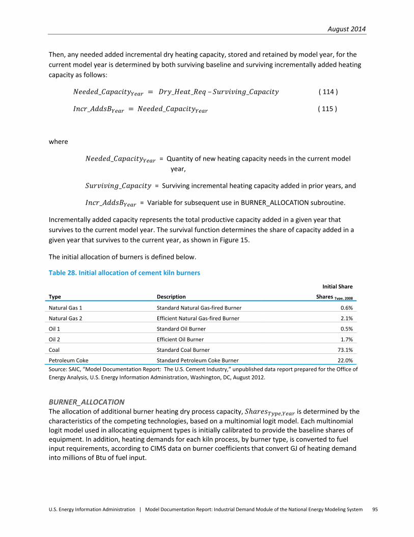
August 2014


Then, any needed added incremental dry heating capacity, stored and retained by model year, for the current model year is determined by both surviving baseline and surviving incrementally added heating capacity as follows:

𝑁𝑒𝑒𝑑𝑒𝑑_𝐶𝑎𝑝𝑎𝑐𝑖𝑡𝑦𝑌𝑒𝑎𝑟 = 𝐷𝑟𝑦_𝐻𝑒𝑎𝑡_𝑅𝑒𝑞 – 𝑆𝑢𝑟𝑣𝑖𝑣𝑖𝑛𝑔_𝐶𝑎𝑝𝑎𝑐𝑖𝑡𝑦 ( 114 )

𝐼𝑛𝑐𝑟_𝐴𝑑𝑑𝑠𝐵𝑌𝑒𝑎𝑟 = 𝑁𝑒𝑒𝑑𝑒𝑑_𝐶𝑎𝑝𝑎𝑐𝑖𝑡𝑦𝑌𝑒𝑎𝑟 ( 115 )

where

𝑁𝑒𝑒𝑑𝑒𝑑_𝐶𝑎𝑝𝑎𝑐𝑖𝑡𝑦𝑌𝑒𝑎𝑟 = Quantity of new heating capacity needs in the current model year,

𝑆𝑢𝑟𝑣𝑖𝑣𝑖𝑛𝑔_𝐶𝑎𝑝𝑎𝑐𝑖𝑡𝑦 = Surviving incremental heating capacity added in prior years, and

𝐼𝑛𝑐𝑟_𝐴𝑑𝑑𝑠𝐵𝑌𝑒𝑎𝑟 = Variable for subsequent use in BURNER_ALLOCATION subroutine.

Incrementally added capacity represents the total productive capacity added in a given year that survives to the current model year. The survival function determines the share of capacity added in a given year that survives to the current year, as shown in Figure 15.

The initial allocation of burners is defined below.

Table 28. Initial allocation of cement kiln burners

Type Description

Initial Share

Shares Type, 2008

Natural Gas 1 Standard Natural Gas-fired Burner 0.6%

Natural Gas 2 Efficient Natural Gas-fired Burner 2.1%

Oil 1 Standard Oil Burner 0.5%

Oil 2 Efficient Oil Burner 1.7%

Coal Standard Coal Burner 73.1%

Petroleum Coke Standard Petroleum Coke Burner 22.0% Source: SAIC, “Model Documentation Report: The U.S. Cement Industry,” unpublished data report prepared for the Office of Energy Analysis, U.S. Energy Information Administration, Washington, DC, August 2012.

BURNER_ALLOCATION The allocation of additional burner heating dry process capacity, 𝑆ℎ𝑎𝑟𝑒𝑠𝑇𝑦𝑝𝑒,𝑌𝑒𝑎𝑟 is determined by the characteristics of the competing technologies, based on a multinomial logit model. Each multinomial logit model used in allocating equipment types is initially calibrated to provide the baseline shares of equipment. In addition, heating demands for each kiln process, by burner type, is converted to fuel input requirements, according to CIMS data on burner coefficients that convert GJ of heating demand into millions of Btu of fuel input.

August 2014


RAW_GRIND_CAP (Node 4)

The clinker output from the kilns in Node 2 governs the required demand in the Raw Grinding step of the CEMENT_INDUSTRY submodule. The model treats the dry and wet processes separately. The quantity of material passing through the raw grinding step is calculated as follows:

𝐷𝑟𝑦_𝑃𝑟𝑜𝑐𝑒𝑠𝑠_𝑂𝑢𝑡 = 𝑃𝑟𝑜𝑐𝑒𝑠𝑠_𝑂𝑢𝑡𝑝𝑢𝑡𝐾 − 𝑊𝑒𝑡_𝑃𝑟𝑜𝑐𝑒𝑠𝑠𝑌𝑒𝑎𝑟 ( 116 )

𝑅𝑎𝑤_𝑀𝑎𝑡𝑒𝑟𝑖𝑎𝑙 = 𝐷𝑟𝑦_𝑃𝑟𝑜𝑐𝑒𝑠𝑠_𝑂𝑢𝑡 ∗ 𝑀𝑎𝑠𝑠𝐿𝑜𝑠𝑠 ( 117 )

where:

𝐷𝑟𝑦_𝑃𝑟𝑜𝑐𝑒𝑠𝑠_𝑂𝑢𝑡 = Quantity of clinker, in thousand metric tons, produced using dry process, as determined from Node 2,

𝑃𝑟𝑜𝑐𝑒𝑠𝑠_𝑂𝑢𝑡𝑝𝑢𝑡𝐾 = Total quantity of clinker, in thousand metric tons, produced as

Determined from Node 2,

𝑊𝑒𝑡_𝑃𝑟𝑜𝑐𝑒𝑠𝑠𝑌𝑒𝑎𝑟 = Quantity of clinker, in thousand metric tons, produced using wet process, as determined from Node 2,

𝑅𝑎𝑤_𝑀𝑎𝑡𝑒𝑟𝑖𝑎𝑙 = Raw material throughput for dry process, in thousands of metric tons, and 𝑀𝑎𝑠𝑠𝐿𝑜𝑠𝑠 = Mass Loss Ratio, set to 1.60.

In 2008, baseline raw grinding capacity is allocated by grinder type in the RAW_GRIND_ALLOC subroutine and computed as follows:

𝐵𝑎𝑠𝑒𝑙𝑖𝑛𝑒_𝐶𝑎𝑝𝑎𝑐𝑖𝑡𝑦𝐼𝐵𝑌𝑅 = 𝑅𝑎𝑤_𝑀𝑎𝑡𝑒𝑟𝑖𝑎𝑙 ( 118 )

𝐵𝑎𝑠𝑒𝑙𝑖𝑛𝑒_𝐶𝑎𝑝𝑎𝑐𝑖𝑡𝑦𝐺2008 = 𝐵𝑎𝑠𝑒𝑙𝑖𝑛𝑒_𝐶𝑎𝑝𝑎𝑐𝑖𝑡𝑦𝐼𝐵𝑌𝑅 ( 119 )

where

𝐵𝑎𝑠𝑒𝑙𝑖𝑛𝑒_𝐶𝑎𝑝𝑎𝑐𝑖𝑡𝑦𝐼𝐵𝑌𝑅 = Baseline heat demand in 2008 for dry process kilns

𝐵𝑎𝑠𝑒𝑙𝑖𝑛𝑒_𝐶𝑎𝑝𝑎𝑐𝑖𝑡𝑦𝐺𝑌𝑒𝑎𝑟 = Burner capacity indexed by 𝑌𝑒𝑎𝑟.

For post-2008 years, the raw material throughputs are determined from baseline retirements and computed as follows:

𝐵𝑎𝑠𝑒𝑙𝑖𝑛𝑒𝐶𝑎𝑝𝑎𝑐𝑖𝑡𝑦𝐺𝑌𝑒𝑎𝑟 =

𝐵𝑎𝑠𝑒𝑙𝑖𝑛𝑒_𝐶𝑎𝑝𝑎𝑐𝑖𝑡𝑦𝐺𝑌𝑒𝑎𝑟−1 − �𝐵𝑎𝑠𝑒𝑙𝑖𝑛𝑒_𝐶𝑎𝑝𝑎𝑐𝑖𝑡𝑦𝐼𝐵𝑌𝑅𝐵𝑎𝑠𝑒𝑙𝑖𝑓𝑒𝑐

� ( 120 )

where

𝐵𝑎𝑠𝑒𝑙𝑖𝑛𝑒_𝐶𝑎𝑝𝑎𝑐𝑖𝑡𝑦𝐺𝑌𝑒𝑎𝑟 = Raw material throughput capacity indexed by 𝑌𝑒𝑎𝑟 and 𝐵𝑎𝑠𝑒𝑙𝑖𝑓𝑒𝑐 = Lifetime of baseline dry process grinding equipment, set to 20 years.

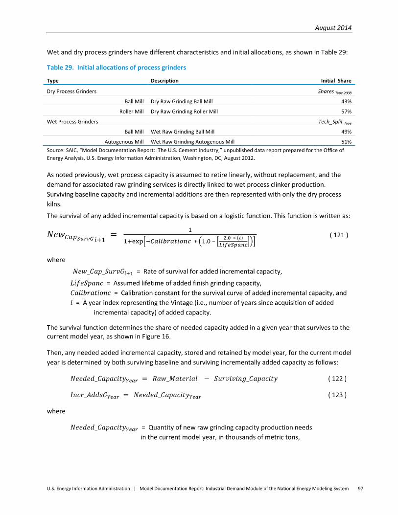
August 2014


Wet and dry process grinders have different characteristics and initial allocations, as shown in Table 29:

Table 29. Initial allocations of process grinders

Type Description Initial Share

Dry Process Grinders Shares Type,2008

Ball Mill Dry Raw Grinding Ball Mill 43%

Roller Mill Dry Raw Grinding Roller Mill 57%

Wet Process Grinders Tech_Split Type

Ball Mill Wet Raw Grinding Ball Mill 49%

Autogenous Mill Wet Raw Grinding Autogenous Mill 51% Source: SAIC, “Model Documentation Report: The U.S. Cement Industry,” unpublished data report prepared for the Office of Energy Analysis, U.S. Energy Information Administration, Washington, DC, August 2012.

As noted previously, wet process capacity is assumed to retire linearly, without replacement, and the demand for associated raw grinding services is directly linked to wet process clinker production. Surviving baseline capacity and incremental additions are then represented with only the dry process kilns.


𝑁𝑒𝑤𝐶𝑎𝑝𝑆𝑢𝑟𝑣𝐺𝑖+1 = 1

1+exp�−𝐶𝑎𝑙𝑖𝑏𝑟𝑎𝑡𝑖𝑜𝑛𝑐 ∗ �1.0 – � 2.0 ∗ (𝑖)𝐿𝑖𝑓𝑒𝑆𝑝𝑎𝑛𝑐��

( 121 )

where

𝑁𝑒𝑤_𝐶𝑎𝑝_𝑆𝑢𝑟𝑣𝐺𝑖+1 = Rate of survival for added incremental capacity,

𝐿𝑖𝑓𝑒𝑆𝑝𝑎𝑛𝑐 = Assumed lifetime of added finish grinding capacity, 𝐶𝑎𝑙𝑖𝑏𝑟𝑎𝑡𝑖𝑜𝑛𝑐 = Calibration constant for the survival curve of added incremental capacity, and 𝑖 = A year index representing the Vintage (i.e., number of years since acquisition of added incremental capacity) of added capacity.


Then, any needed added incremental capacity, stored and retained by model year, for the current model year is determined by both surviving baseline and surviving incrementally added capacity as follows:

𝑁𝑒𝑒𝑑𝑒𝑑_𝐶𝑎𝑝𝑎𝑐𝑖𝑡𝑦𝑌𝑒𝑎𝑟 = 𝑅𝑎𝑤_𝑀𝑎𝑡𝑒𝑟𝑖𝑎𝑙 − 𝑆𝑢𝑟𝑣𝑖𝑣𝑖𝑛𝑔_𝐶𝑎𝑝𝑎𝑐𝑖𝑡𝑦 ( 122 )

𝐼𝑛𝑐𝑟_𝐴𝑑𝑑𝑠𝐺𝑌𝑒𝑎𝑟 = 𝑁𝑒𝑒𝑑𝑒𝑑_𝐶𝑎𝑝𝑎𝑐𝑖𝑡𝑦𝑌𝑒𝑎𝑟 ( 123 )

where

𝑁𝑒𝑒𝑑𝑒𝑑_𝐶𝑎𝑝𝑎𝑐𝑖𝑡𝑦𝑌𝑒𝑎𝑟 = Quantity of new raw grinding capacity production needs in the current model year, in thousands of metric tons,

August 2014


𝑅𝑎𝑤_𝑀𝑎𝑡𝑒𝑟𝑖𝑎𝑙 = Raw material throughput for dry process, in thousands of metric tons , 𝑆𝑢𝑟𝑣𝑖𝑣𝑖𝑛𝑔_𝐶𝑎𝑝𝑎𝑐𝑖𝑡𝑦 = Surviving incremental capacity added in prior years, and 𝐼𝑛𝑐𝑟_𝐴𝑑𝑑𝑠𝐺𝑌𝑒𝑎𝑟 = Variable for subsequent use in RAW_GRIND_ALLOC subroutine.


The use of the wet process is considered to be declining, and is consequently not subject to replacement by new, similar technologies. Because of different input process (e.g., raw grinding) requirements associated with the wet process, it needs to be tracked separately, and retirements are accommodated by additions to dry process technology. Any added incremental capacities for dry rotary kilns are subsequently allocated to raw grinder Type in the RAW_GRIND_ALLOC subroutine.

RAW_GRIND_ALLOC The allocation of additional raw grinding capacity, 𝑆ℎ𝑎𝑟𝑒𝑠𝑇𝑦𝑝𝑒,𝑌𝑒𝑎𝑟 is determined by the characteristics of the competing technologies, based on a multinomial logit model. Each multinomial logit model used in allocating equipment types is initially calibrated to provide the baseline shares of equipment.

The energy projected and then reported in the IDM for raw grinding is determined from the raw material throughput and energy intensity of each type of raw grinder, as reported in the CIMS data, which subsequently is partitioned into Census Regions in the CALPATOT subroutine of IDM.

Process Emissions Calculations Process emissions are significant during clinker production at cement manufacturers. IDM computes these process emissions as follows:

Process-related emissions are calculated using empirical relationships from the U.S. Environmental Protection Agency that link the emissions of CO2 (process-related) and cement kiln dust (CKD) with the amount of raw material entering the kiln. Process-related CO2 emissions are computed for each ton of clinker produced, while CKD emissions are calculated based on each ton of cement produced. Note that CKD emissions are typically recycled with a 2% loss.37 A standard emissions factor (0.51 tons of carbon dioxide per ton of clinker) is used to calculate process-related CO2 emissions. When raw material additives, such as blast furnace slag, are used, the emissions factor drops to 0.50 tons of CO2 per ton of clinker.

Fuel-related CO2 emissions are calculated from the portfolio of fuels used by the cement industry over a given year. These are calculated in the IDM and added to the amount of process-based CO2 emissions described above.

37 Huntzinger et al, Life Cycle Analyses of Portland Cement Manufacture, J. of Cleaner Production, 17 (2009) pp. 668-675.

August 2014


LIME_INDUSTRY Submodule The lime industry submodule calculates lime industry energy consumption. Cement and lime energy shipments and energy consumption are reported together, although they are projected separately. The new process flow model calculates UEC as a function of capital equipment used and updates capital equipment based on demand, capacity surviving, and new capacity. Domestic lime production is not directly estimated by the MAM. However, the MAM macro variable MC_REVIND(11,20,Year), which denotes gross output from “Other Nonmetallic Mineral Products,” is used as a proxy for lime production when calculating CO2 emissions. Accordingly, this variable is also used to estimate the metric tons of lime production in the projected years. This is done by indexing the macro variable to its 2009 value (the last year for which total lime production was published by USGS), and adjusting the 2009 production value to apply to each projection year, as shown below. This provides a time series estimate of lime production throughout the forecast. Internal submodule calculations are in metric units, which are converted to English units for calculations external to this submodule.

The physical quantity of lime kiln outputs (i.e., shipments) is the total quantity of shipments (in thousand metric tons) in a given year.

𝐷𝑒𝑚𝑎𝑛𝑑 = 𝐷𝑒𝑚𝑎𝑛𝑑_𝐼𝐵𝑌𝑅2 ∗ �𝑂𝑈𝑇𝐼𝑁𝐷23,11

𝐿𝐼𝑀𝐸𝐼𝐵𝑌𝑅� ( 124 )

where

𝐷𝑒𝑚𝑎𝑛𝑑 = Physical quantity of lime shipments, in thousands of metric tons, projected for the lime industry, as reported by the U.S. Department of Interior, U.S. Geological Survey;

𝐷𝑒𝑚𝑎𝑛𝑑_𝐼𝐵𝑌𝑅2 = Physical quantity of lime shipments, in thousands of metric tons in 2009, as reported by the U.S. Department of Interior, U.S. Geological Survey;

𝑂𝑈𝑇𝐼𝑁𝐷23,11 = Gross value of output for the lime industry (IDM industry code of 23) for the nation in the current projection year, as determined by NEMS MAM and internally adjusted by IDM; and

𝐿𝐼𝑀𝐸𝐼𝐵𝑌𝑅 = Gross value of output for the lime industry for the nation in year 2009, as determined by MAM and internally adjusted by IDM.

The initial, 2009 value of lime production is obtained from the USGS Data Series 140, and is estimated at 15,800 thousand metric tons. Projected values are determined by applying the associated macroeconomic index. The energy required for processing this output is determined by the existing and projected future stock of lime kilns, as discussed below.

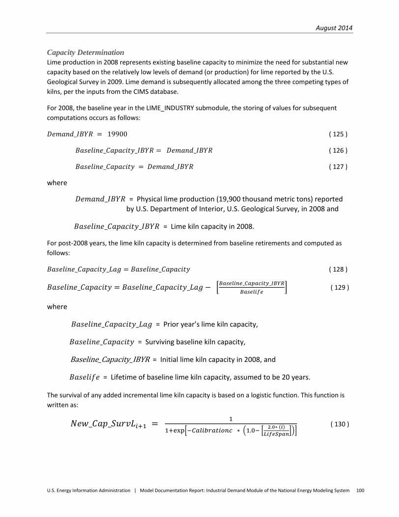
August 2014


Capacity Determination Lime production in 2008 represents existing baseline capacity to minimize the need for substantial new capacity based on the relatively low levels of demand (or production) for lime reported by the U.S. Geological Survey in 2009. Lime demand is subsequently allocated among the three competing types of kilns, per the inputs from the CIMS database.

For 2008, the baseline year in the LIME_INDUSTRY submodule, the storing of values for subsequent computations occurs as follows:

𝐷𝑒𝑚𝑎𝑛𝑑_𝐼𝐵𝑌𝑅 = 19900 ( 125 )

𝐵𝑎𝑠𝑒𝑙𝑖𝑛𝑒_𝐶𝑎𝑝𝑎𝑐𝑖𝑡𝑦_𝐼𝐵𝑌𝑅 = 𝐷𝑒𝑚𝑎𝑛𝑑_𝐼𝐵𝑌𝑅 ( 126 )

𝐵𝑎𝑠𝑒𝑙𝑖𝑛𝑒_𝐶𝑎𝑝𝑎𝑐𝑖𝑡𝑦 = 𝐷𝑒𝑚𝑎𝑛𝑑_𝐼𝐵𝑌𝑅 ( 127 )

where

𝐷𝑒𝑚𝑎𝑛𝑑_𝐼𝐵𝑌𝑅 = Physical lime production (19,900 thousand metric tons) reported by U.S. Department of Interior, U.S. Geological Survey, in 2008 and

𝐵𝑎𝑠𝑒𝑙𝑖𝑛𝑒_𝐶𝑎𝑝𝑎𝑐𝑖𝑡𝑦_𝐼𝐵𝑌𝑅 = Lime kiln capacity in 2008.

For post-2008 years, the lime kiln capacity is determined from baseline retirements and computed as follows:

𝐵𝑎𝑠𝑒𝑙𝑖𝑛𝑒_𝐶𝑎𝑝𝑎𝑐𝑖𝑡𝑦_𝐿𝑎𝑔 = 𝐵𝑎𝑠𝑒𝑙𝑖𝑛𝑒_𝐶𝑎𝑝𝑎𝑐𝑖𝑡𝑦 ( 128 )

𝐵𝑎𝑠𝑒𝑙𝑖𝑛𝑒_𝐶𝑎𝑝𝑎𝑐𝑖𝑡𝑦 = 𝐵𝑎𝑠𝑒𝑙𝑖𝑛𝑒_𝐶𝑎𝑝𝑎𝑐𝑖𝑡𝑦_𝐿𝑎𝑔 − �𝐵𝑎𝑠𝑒𝑙𝑖𝑛𝑒_𝐶𝑎𝑝𝑎𝑐𝑖𝑡𝑦_𝐼𝐵𝑌𝑅𝐵𝑎𝑠𝑒𝑙𝑖𝑓𝑒

� ( 129 )

where

𝐵𝑎𝑠𝑒𝑙𝑖𝑛𝑒_𝐶𝑎𝑝𝑎𝑐𝑖𝑡𝑦_𝐿𝑎𝑔 = Prior year’s lime kiln capacity,

𝐵𝑎𝑠𝑒𝑙𝑖𝑛𝑒_𝐶𝑎𝑝𝑎𝑐𝑖𝑡𝑦 = Surviving baseline kiln capacity,

Baseline_Capacity_IBYR = Initial lime kiln capacity in 2008, and

𝐵𝑎𝑠𝑒𝑙𝑖𝑓𝑒 = Lifetime of baseline lime kiln capacity, assumed to be 20 years.

The survival of any added incremental lime kiln capacity is based on a logistic function. This function is written as:

𝑁𝑒𝑤_𝐶𝑎𝑝_𝑆𝑢𝑟𝑣𝐿𝑖+1 = 1

1+exp�−𝐶𝑎𝑙𝑖𝑏𝑟𝑎𝑡𝑖𝑜𝑛𝑐 ∗ �1.0− � 2.0∗ (𝑖)𝐿𝑖𝑓𝑒𝑆𝑝𝑎𝑛��

( 130 )

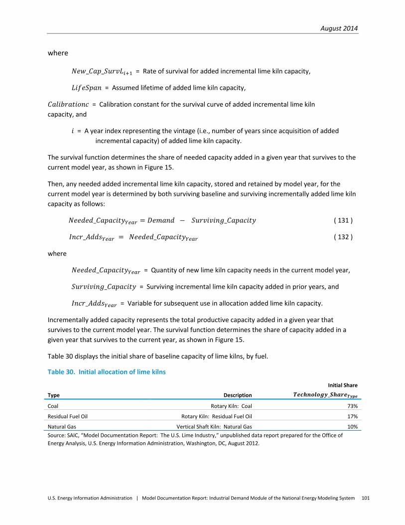
August 2014


where

𝑁𝑒𝑤_𝐶𝑎𝑝_𝑆𝑢𝑟𝑣𝐿𝑖+1 = Rate of survival for added incremental lime kiln capacity,

𝐿𝑖𝑓𝑒𝑆𝑝𝑎𝑛 = Assumed lifetime of added lime kiln capacity,

𝐶𝑎𝑙𝑖𝑏𝑟𝑎𝑡𝑖𝑜𝑛𝑐 = Calibration constant for the survival curve of added incremental lime kiln capacity, and

𝑖 = A year index representing the vintage (i.e., number of years since acquisition of added incremental capacity) of added lime kiln capacity.


Then, any needed added incremental lime kiln capacity, stored and retained by model year, for the current model year is determined by both surviving baseline and surviving incrementally added lime kiln capacity as follows:

𝑁𝑒𝑒𝑑𝑒𝑑_𝐶𝑎𝑝𝑎𝑐𝑖𝑡𝑦𝑌𝑒𝑎𝑟 = 𝐷𝑒𝑚𝑎𝑛𝑑 − 𝑆𝑢𝑟𝑣𝑖𝑣𝑖𝑛𝑔_𝐶𝑎𝑝𝑎𝑐𝑖𝑡𝑦 ( 131 )

𝐼𝑛𝑐𝑟_𝐴𝑑𝑑𝑠𝑌𝑒𝑎𝑟 = 𝑁𝑒𝑒𝑑𝑒𝑑_𝐶𝑎𝑝𝑎𝑐𝑖𝑡𝑦𝑌𝑒𝑎𝑟 ( 132 )

where

𝑁𝑒𝑒𝑑𝑒𝑑_𝐶𝑎𝑝𝑎𝑐𝑖𝑡𝑦𝑌𝑒𝑎𝑟 = Quantity of new lime kiln capacity needs in the current model year,

𝑆𝑢𝑟𝑣𝑖𝑣𝑖𝑛𝑔_𝐶𝑎𝑝𝑎𝑐𝑖𝑡𝑦 = Surviving incremental lime kiln capacity added in prior years, and

𝐼𝑛𝑐𝑟_𝐴𝑑𝑑𝑠𝑌𝑒𝑎𝑟 = Variable for subsequent use in allocation added lime kiln capacity.


Table 30 displays the initial share of baseline capacity of lime kilns, by fuel.

Table 30. Initial allocation of lime kilns

Type Description

Initial Share 𝑻𝒆𝒄𝒉𝒏𝒐𝒍𝒐𝒈𝒚_𝑺𝒉𝒂𝒓𝒆𝑻𝒚𝒑𝒆

Coal Rotary Kiln: Coal 73%

Residual Fuel Oil Rotary Kiln: Residual Fuel Oil 17%

Natural Gas Vertical Shaft Kiln: Natural Gas 10% Source: SAIC, “Model Documentation Report: The U.S. Lime Industry,” unpublished data report prepared for the Office of Energy Analysis, U.S. Energy Information Administration, Washington, DC, August 2012.

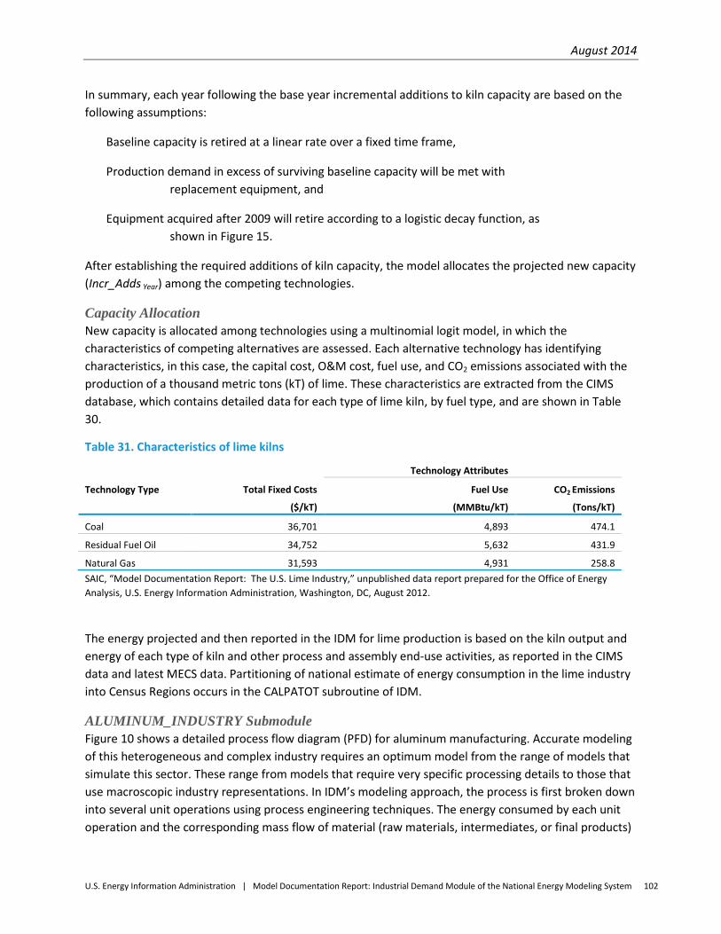
August 2014


In summary, each year following the base year incremental additions to kiln capacity are based on the following assumptions:

Baseline capacity is retired at a linear rate over a fixed time frame,

Production demand in excess of surviving baseline capacity will be met with replacement equipment, and

Equipment acquired after 2009 will retire according to a logistic decay function, as shown in Figure 15.

After establishing the required additions of kiln capacity, the model allocates the projected new capacity (Incr_Adds Year) among the competing technologies.

Capacity Allocation New capacity is allocated among technologies using a multinomial logit model, in which the characteristics of competing alternatives are assessed. Each alternative technology has identifying characteristics, in this case, the capital cost, O&M cost, fuel use, and CO2 emissions associated with the production of a thousand metric tons (kT) of lime. These characteristics are extracted from the CIMS database, which contains detailed data for each type of lime kiln, by fuel type, and are shown in Table 30.

Table 31. Characteristics of lime kilns

Technology Attributes

Technology Type Total Fixed Costs

($/kT)

Fuel Use

(MMBtu/kT)

CO2 Emissions

(Tons/kT)

Coal 36,701 4,893 474.1

Residual Fuel Oil 34,752 5,632 431.9

Natural Gas 31,593 4,931 258.8 SAIC, “Model Documentation Report: The U.S. Lime Industry,” unpublished data report prepared for the Office of Energy Analysis, U.S. Energy Information Administration, Washington, DC, August 2012.

The energy projected and then reported in the IDM for lime production is based on the kiln output and energy of each type of kiln and other process and assembly end-use activities, as reported in the CIMS data and latest MECS data. Partitioning of national estimate of energy consumption in the lime industry into Census Regions occurs in the CALPATOT subroutine of IDM.

ALUMINUM_INDUSTRY Submodule Figure 10 shows a detailed process flow diagram (PFD) for aluminum manufacturing. Accurate modeling of this heterogeneous and complex industry requires an optimum model from the range of models that simulate this sector. These range from models that require very specific processing details to those that use macroscopic industry representations. In IDM’s modeling approach, the process is first broken down into several unit operations using process engineering techniques. The energy consumed by each unit operation and the corresponding mass flow of material (raw materials, intermediates, or final products)

August 2014


through that unit operation are calculated from the data. Their ratio supplies the UEC specific for that unit operation. The energy demands for processing the required mass of material through each unit operation are calculated and aggregated to provide the total energy consumption for the desired amount of the product(s). By virtue of its ability to calculate energy demands at the unit operation level, the aggregated estimate is a more accurate calculation of energy consumption compared with that from a global UEC. This approach is discussed in detail in the ensuing sections, starting with a description of the aluminum manufacturing process.

Background on aluminum industry The U.S. aluminum industry is a broadly diversified industry, starting with ore refining and ending with a wide variety of industrial and consumer products.38 Aluminum (Al) is the third most abundant element in the earth's crust, but does not occur in nature as a metal, but only as an oxide (alumina), which in turn, is found in an ore called bauxite. In recent years, aluminum has begun to replace iron and steel in the automotive, electric power, and construction industries owing to its lighter weight, resistance to rust, alloyability, and recyclability. It is popular as a packaging material for beverages and food containers, as well as household and institutional foil.

The supply of aluminum in the United States stems from three basic sources: Primary production - domestic production from aluminum ore. Secondary production – domestic metal recovered from scrap, a.k.a. recycling Imports - primary and secondary ingots and mill products

The end product from the first two sources is molten aluminum metal, which is not in a form suitable for marketing to potential end-users. Instead, ingot casting is the vital conduit between the molten metal and the manufacture of aluminum and aluminum alloy products. Extrusions, forgings, sheet, plate, and foil begin as billet and fabricating ingots. Sand, permanent mold, investment, and pressure die castings typically originate in alloyed remelt ingots. For this modeling effort, it is assumed that aluminum imports are also processed like primary and secondary aluminum into end-use products.

Currently there are over 400 wrought aluminum and wrought aluminum alloys and over 200 aluminum alloys in the form of castings and ingots to match the wide range of material characteristics required by end-use manufacturing processes.39 In some cases, ingot formation and the manufacture of the final aluminum product for end-use applications are in the same location.

ALUMINUM_INDUSTRY Submodule: Subroutines For this modeling effort, the boundaries established for the macroscopic modeling of the aluminum industry begin with the delivery of bauxite or scrap aluminum at the plant gate and end with ingot formation and the manufacture of aluminum sheet, plate, foil, and extruded products. Aluminum foundry operations for die and non-die casting are included.

38 All bauxite for primary production is assumed imported to the United States. 39 For aluminum specifications, see the Aluminum Association, http://www.aluminum.org/Content/NavigationMenu/TheIndustry/IndustryStandards/Teal_Sheets.pdf.

http://www.aluminum.org/Content/NavigationMenu/TheIndustry/IndustryStandards/Teal_Sheets.pdf

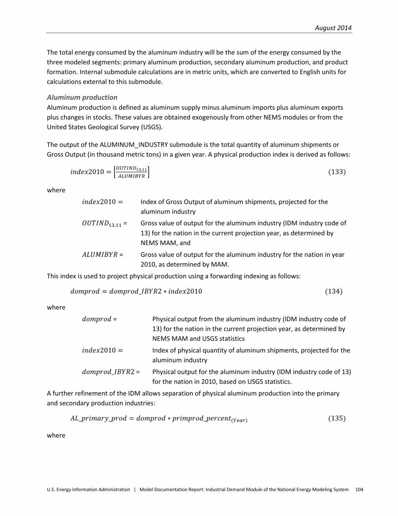
August 2014


The total energy consumed by the aluminum industry will be the sum of the energy consumed by the three modeled segments: primary aluminum production, secondary aluminum production, and product formation. Internal submodule calculations are in metric units, which are converted to English units for calculations external to this submodule.

Aluminum production Aluminum production is defined as aluminum supply minus aluminum imports plus aluminum exports plus changes in stocks. These values are obtained exogenously from other NEMS modules or from the United States Geological Survey (USGS).

The output of the ALUMINUM_INDUSTRY submodule is the total quantity of aluminum shipments or Gross Output (in thousand metric tons) in a given year. A physical production index is derived as follows:

𝑖𝑛𝑑𝑒𝑥2010 = �𝑂𝑈𝑇𝐼𝑁𝐷13,11𝐴𝐿𝑈𝑀𝐼𝐵𝑌𝑅

� (133)

where

𝑖𝑛𝑑𝑒𝑥2010 = Index of Gross Output of aluminum shipments, projected for the aluminum industry

𝑂𝑈𝑇𝐼𝑁𝐷13,11 = Gross value of output for the aluminum industry (IDM industry code of 13) for the nation in the current projection year, as determined by NEMS MAM, and

𝐴𝐿𝑈𝑀𝐼𝐵𝑌𝑅 = Gross value of output for the aluminum industry for the nation in year 2010, as determined by MAM.

This index is used to project physical production using a forwarding indexing as follows:

𝑑𝑜𝑚𝑝𝑟𝑜𝑑 = 𝑑𝑜𝑚𝑝𝑟𝑜𝑑_𝐼𝐵𝑌𝑅2 ∗ 𝑖𝑛𝑑𝑒𝑥2010 (134)

where

𝑑𝑜𝑚𝑝𝑟𝑜𝑑 = Physical output from the aluminum industry (IDM industry code of 13) for the nation in the current projection year, as determined by NEMS MAM and USGS statistics

𝑖𝑛𝑑𝑒𝑥2010 = Index of physical quantity of aluminum shipments, projected for the aluminum industry

𝑑𝑜𝑚𝑝𝑟𝑜𝑑_𝐼𝐵𝑌𝑅2 = Physical output for the aluminum industry (IDM industry code of 13) for the nation in 2010, based on USGS statistics.

A further refinement of the IDM allows separation of physical aluminum production into the primary and secondary production industries:

𝐴𝐿_𝑝𝑟𝑖𝑚𝑎𝑟𝑦_𝑝𝑟𝑜𝑑 = 𝑑𝑜𝑚𝑝𝑟𝑜𝑑 ∗ 𝑝𝑟𝑖𝑚𝑝𝑟𝑜𝑑_𝑝𝑒𝑟𝑐𝑒𝑛𝑡(𝑌𝑒𝑎𝑟) (135)

where

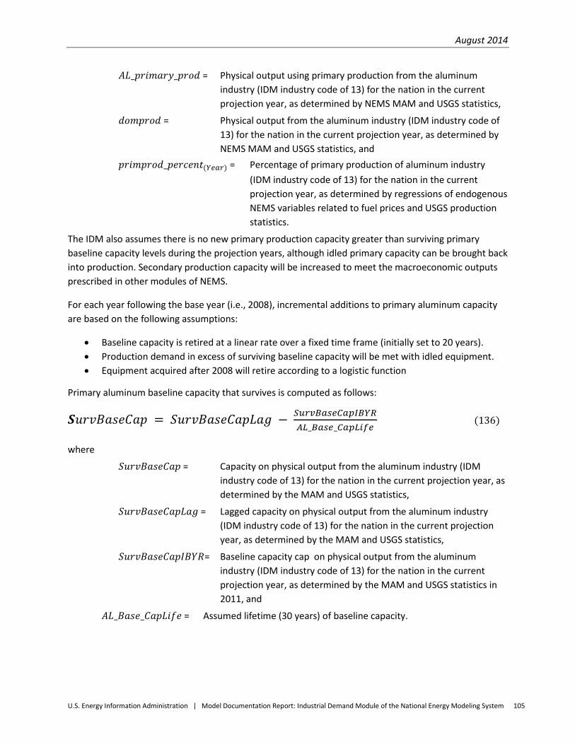
August 2014


𝐴𝐿_𝑝𝑟𝑖𝑚𝑎𝑟𝑦_𝑝𝑟𝑜𝑑 = Physical output using primary production from the aluminum industry (IDM industry code of 13) for the nation in the current projection year, as determined by NEMS MAM and USGS statistics,

𝑑𝑜𝑚𝑝𝑟𝑜𝑑 = Physical output from the aluminum industry (IDM industry code of 13) for the nation in the current projection year, as determined by NEMS MAM and USGS statistics, and

𝑝𝑟𝑖𝑚𝑝𝑟𝑜𝑑_𝑝𝑒𝑟𝑐𝑒𝑛𝑡(𝑌𝑒𝑎𝑟) = Percentage of primary production of aluminum industry (IDM industry code of 13) for the nation in the current projection year, as determined by regressions of endogenous NEMS variables related to fuel prices and USGS production statistics.

The IDM also assumes there is no new primary production capacity greater than surviving primary baseline capacity levels during the projection years, although idled primary capacity can be brought back into production. Secondary production capacity will be increased to meet the macroeconomic outputs prescribed in other modules of NEMS.

For each year following the base year (i.e., 2008), incremental additions to primary aluminum capacity are based on the following assumptions:

• Baseline capacity is retired at a linear rate over a fixed time frame (initially set to 20 years). • Production demand in excess of surviving baseline capacity will be met with idled equipment. • Equipment acquired after 2008 will retire according to a logistic function

Primary aluminum baseline capacity that survives is computed as follows:

𝑺𝑢𝑟𝑣𝐵𝑎𝑠𝑒𝐶𝑎𝑝 = 𝑆𝑢𝑟𝑣𝐵𝑎𝑠𝑒𝐶𝑎𝑝𝐿𝑎𝑔 − 𝑆𝑢𝑟𝑣𝐵𝑎𝑠𝑒𝐶𝑎𝑝𝐼𝐵𝑌𝑅𝐴𝐿_𝐵𝑎𝑠𝑒_𝐶𝑎𝑝𝐿𝑖𝑓𝑒

(136)

where

𝑆𝑢𝑟𝑣𝐵𝑎𝑠𝑒𝐶𝑎𝑝 = Capacity on physical output from the aluminum industry (IDM industry code of 13) for the nation in the current projection year, as determined by the MAM and USGS statistics,

𝑆𝑢𝑟𝑣𝐵𝑎𝑠𝑒𝐶𝑎𝑝𝐿𝑎𝑔 = Lagged capacity on physical output from the aluminum industry (IDM industry code of 13) for the nation in the current projection year, as determined by the MAM and USGS statistics,

𝑆𝑢𝑟𝑣𝐵𝑎𝑠𝑒𝐶𝑎𝑝𝐼𝐵𝑌𝑅= Baseline capacity cap on physical output from the aluminum industry (IDM industry code of 13) for the nation in the current projection year, as determined by the MAM and USGS statistics in 2011, and

𝐴𝐿_𝐵𝑎𝑠𝑒_𝐶𝑎𝑝𝐿𝑖𝑓𝑒 = Assumed lifetime (30 years) of baseline capacity.

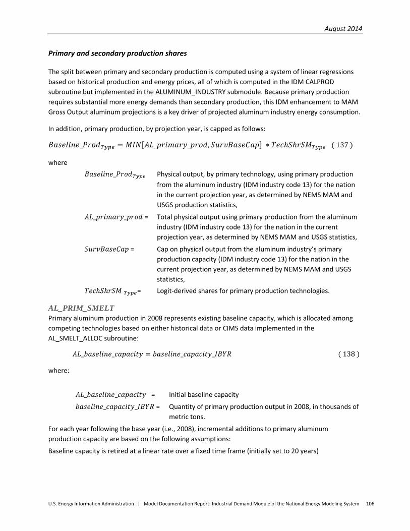
August 2014


Primary and secondary production shares

The split between primary and secondary production is computed using a system of linear regressions based on historical production and energy prices, all of which is computed in the IDM CALPROD subroutine but implemented in the ALUMINUM_INDUSTRY submodule. Because primary production requires substantial more energy demands than secondary production, this IDM enhancement to MAM Gross Output aluminum projections is a key driver of projected aluminum industry energy consumption.

In addition, primary production, by projection year, is capped as follows:

𝐵𝑎𝑠𝑒𝑙𝑖𝑛𝑒_𝑃𝑟𝑜𝑑𝑇𝑦𝑝𝑒 = 𝑀𝐼𝑁[𝐴𝐿_𝑝𝑟𝑖𝑚𝑎𝑟𝑦_𝑝𝑟𝑜𝑑, 𝑆𝑢𝑟𝑣𝐵𝑎𝑠𝑒𝐶𝑎𝑝] ∗ 𝑇𝑒𝑐ℎ𝑆ℎ𝑟𝑆𝑀𝑇𝑦𝑝𝑒 ( 137 )

where 𝐵𝑎𝑠𝑒𝑙𝑖𝑛𝑒_𝑃𝑟𝑜𝑑𝑇𝑦𝑝𝑒 Physical output, by primary technology, using primary production

from the aluminum industry (IDM industry code 13) for the nation in the current projection year, as determined by NEMS MAM and USGS production statistics,

𝐴𝐿_𝑝𝑟𝑖𝑚𝑎𝑟𝑦_𝑝𝑟𝑜𝑑 = Total physical output using primary production from the aluminum industry (IDM industry code 13) for the nation in the current projection year, as determined by NEMS MAM and USGS statistics,

𝑆𝑢𝑟𝑣𝐵𝑎𝑠𝑒𝐶𝑎𝑝 = Cap on physical output from the aluminum industry’s primary production capacity (IDM industry code 13) for the nation in the current projection year, as determined by NEMS MAM and USGS statistics,

𝑇𝑒𝑐ℎ𝑆ℎ𝑟𝑆𝑀 𝑇𝑦𝑝𝑒= Logit-derived shares for primary production technologies.

AL_PRIM_SMELT Primary aluminum production in 2008 represents existing baseline capacity, which is allocated among competing technologies based on either historical data or CIMS data implemented in the AL_SMELT_ALLOC subroutine:

𝐴𝐿_𝑏𝑎𝑠𝑒𝑙𝑖𝑛𝑒_𝑐𝑎𝑝𝑎𝑐𝑖𝑡𝑦 = 𝑏𝑎𝑠𝑒𝑙𝑖𝑛𝑒_𝑐𝑎𝑝𝑎𝑐𝑖𝑡𝑦_𝐼𝐵𝑌𝑅 ( 138 )

where:

𝐴𝐿_𝑏𝑎𝑠𝑒𝑙𝑖𝑛𝑒_𝑐𝑎𝑝𝑎𝑐𝑖𝑡𝑦 = Initial baseline capacity

𝑏𝑎𝑠𝑒𝑙𝑖𝑛𝑒_𝑐𝑎𝑝𝑎𝑐𝑖𝑡𝑦_𝐼𝐵𝑌𝑅 = Quantity of primary production output in 2008, in thousands of metric tons.

For each year following the base year (i.e., 2008), incremental additions to primary aluminum production capacity are based on the following assumptions:

Baseline capacity is retired at a linear rate over a fixed time frame (initially set to 20 years)

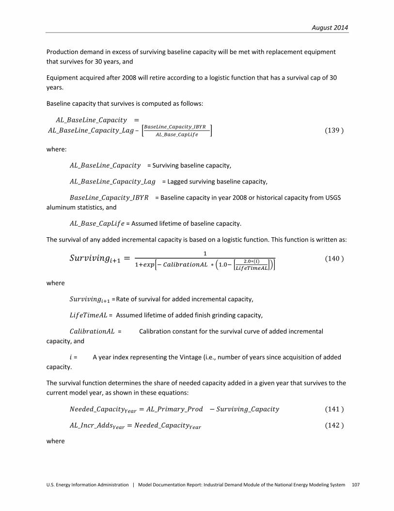
August 2014


Production demand in excess of surviving baseline capacity will be met with replacement equipment that survives for 30 years, and

Equipment acquired after 2008 will retire according to a logistic function that has a survival cap of 30 years.

Baseline capacity that survives is computed as follows:

𝐴𝐿_𝐵𝑎𝑠𝑒𝐿𝑖𝑛𝑒_𝐶𝑎𝑝𝑎𝑐𝑖𝑡𝑦 = 𝐴𝐿_𝐵𝑎𝑠𝑒𝐿𝑖𝑛𝑒_𝐶𝑎𝑝𝑎𝑐𝑖𝑡𝑦_𝐿𝑎𝑔 – �𝐵𝑎𝑠𝑒𝐿𝑖𝑛𝑒_𝐶𝑎𝑝𝑎𝑐𝑖𝑡𝑦_𝐼𝐵𝑌𝑅

𝐴𝐿_𝐵𝑎𝑠𝑒_𝐶𝑎𝑝𝐿𝑖𝑓𝑒� (139 )

where:

𝐴𝐿_𝐵𝑎𝑠𝑒𝐿𝑖𝑛𝑒_𝐶𝑎𝑝𝑎𝑐𝑖𝑡𝑦 = Surviving baseline capacity,

𝐴𝐿_𝐵𝑎𝑠𝑒𝐿𝑖𝑛𝑒_𝐶𝑎𝑝𝑎𝑐𝑖𝑡𝑦_𝐿𝑎𝑔 = Lagged surviving baseline capacity,

𝐵𝑎𝑠𝑒𝐿𝑖𝑛𝑒_𝐶𝑎𝑝𝑎𝑐𝑖𝑡𝑦_𝐼𝐵𝑌𝑅 = Baseline capacity in year 2008 or historical capacity from USGS aluminum statistics, and

𝐴𝐿_𝐵𝑎𝑠𝑒_𝐶𝑎𝑝𝐿𝑖𝑓𝑒 = Assumed lifetime of baseline capacity.


𝑆𝑢𝑟𝑣𝑖𝑣𝑖𝑛𝑔𝑖+1 = 1

1+𝑒𝑥𝑝�− 𝐶𝑎𝑙𝑖𝑏𝑟𝑎𝑡𝑖𝑜𝑛𝐴𝐿 ∗ �1.0− � 2.0∗(𝑖)𝐿𝑖𝑓𝑒𝑇𝑖𝑚𝑒𝐴𝐿��

(140 )

where

𝑆𝑢𝑟𝑣𝑖𝑣𝑖𝑛𝑔𝑖+1 = Rate of survival for added incremental capacity,

𝐿𝑖𝑓𝑒𝑇𝑖𝑚𝑒𝐴𝐿 = Assumed lifetime of added finish grinding capacity,

𝐶𝑎𝑙𝑖𝑏𝑟𝑎𝑡𝑖𝑜𝑛𝐴𝐿 = Calibration constant for the survival curve of added incremental capacity, and

𝑖 = A year index representing the Vintage (i.e., number of years since acquisition of added capacity.

The survival function determines the share of needed capacity added in a given year that survives to the current model year, as shown in these equations:

𝑁𝑒𝑒𝑑𝑒𝑑_𝐶𝑎𝑝𝑎𝑐𝑖𝑡𝑦𝑌𝑒𝑎𝑟 = 𝐴𝐿_𝑃𝑟𝑖𝑚𝑎𝑟𝑦_𝑃𝑟𝑜𝑑 − 𝑆𝑢𝑟𝑣𝑖𝑣𝑖𝑛𝑔_𝐶𝑎𝑝𝑎𝑐𝑖𝑡𝑦 (141 )

𝐴𝐿_𝐼𝑛𝑐𝑟_𝐴𝑑𝑑𝑠𝑌𝑒𝑎𝑟 = 𝑁𝑒𝑒𝑑𝑒𝑑_𝐶𝑎𝑝𝑎𝑐𝑖𝑡𝑦𝑌𝑒𝑎𝑟 (142 )

where

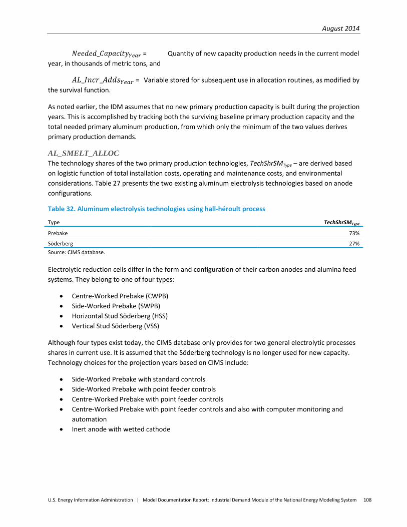
August 2014


𝑁𝑒𝑒𝑑𝑒𝑑_𝐶𝑎𝑝𝑎𝑐𝑖𝑡𝑦𝑌𝑒𝑎𝑟 = Quantity of new capacity production needs in the current model year, in thousands of metric tons, and

𝐴𝐿_𝐼𝑛𝑐𝑟_𝐴𝑑𝑑𝑠𝑌𝑒𝑎𝑟 = Variable stored for subsequent use in allocation routines, as modified by the survival function.

As noted earlier, the IDM assumes that no new primary production capacity is built during the projection years. This is accomplished by tracking both the surviving baseline primary production capacity and the total needed primary aluminum production, from which only the minimum of the two values derives primary production demands.

AL_SMELT_ALLOC The technology shares of the two primary production technologies, TechShrSMType – are derived based on logistic function of total installation costs, operating and maintenance costs, and environmental considerations. Table 27 presents the two existing aluminum electrolysis technologies based on anode configurations.

Table 32. Aluminum electrolysis technologies using hall-héroult process

Type TechShrSMType Prebake 73%

Söderberg 27% Source: CIMS database.

Electrolytic reduction cells differ in the form and configuration of their carbon anodes and alumina feed systems. They belong to one of four types:

• Centre-Worked Prebake (CWPB) • Side-Worked Prebake (SWPB) • Horizontal Stud Söderberg (HSS) • Vertical Stud Söderberg (VSS)

Although four types exist today, the CIMS database only provides for two general electrolytic processes shares in current use. It is assumed that the Söderberg technology is no longer used for new capacity. Technology choices for the projection years based on CIMS include:

• Side-Worked Prebake with standard controls • Side-Worked Prebake with point feeder controls • Centre-Worked Prebake with point feeder controls • Centre-Worked Prebake with point feeder controls and also with computer monitoring and

automation • Inert anode with wetted cathode

August 2014


Remaining ALUMINUM_INDUSTRY Submodule Subroutines

For the remaining subroutines that make up the ALUMINUM_INDUSTRY submodule, similar computations on capacity and allocation by technology diffusion are completed in subroutines AL_ANODE_PRD (i.e., anode production), AL_PRIM_ALUMINA (i.e., alumina production), AL_ALLOC (i.e., alumina allocations), AL_SEC_PRD (i.e., secondary production), and AL_SEC_ALLOC (i.e., secondary technology allocation). Outputs from these routines – e.g., respective projected production levels by technology – are linked with the technology-specific energy demands from the CIMS database to allow computation and reporting of energy consumption in the aluminum industry.

Influence of Electricity Price on Aluminum Production

In addition to the process flow model described above, the Industrial Demand Module also incorporates a regression-based modifier to allow the electricity price to help drive the choice between primary or secondary production. Primary production involves electrochemical smelting of alumina and is very electricity-intensive as compared to the more natural gas-intensive secondary (recycled) aluminum production, and so the industrial electricity price can play a role in the production pathways choice. A regression was performed with historical primary: secondary ratio against industrial electricity prices (both current and lagged).

𝐴𝐿𝑅𝐴𝑇𝐼𝑂𝑟 = 𝑃𝐶𝑅𝑋𝑟,𝑓=2 ∗ 𝐴𝐿𝑆𝐿𝑂𝑃𝐸𝑟 + 𝑃𝐶𝑅𝑋𝐿𝐴𝐺𝑟,𝑓=2 ∗ 𝐴𝐿𝑆𝐿𝑂𝑃𝐸𝐿𝐴𝐺𝑟 + 𝐴𝐿𝐼𝑁𝑇𝐸𝑅𝐶𝐸𝑃𝑇𝑟 ( 143 ) where

𝑃𝐶𝑅𝑋𝑟,𝑓 = the industrial electricity price (f=2), by region r

𝑃𝐶𝑅𝑋𝐿𝐴𝐺𝑟,𝑓 =the lagged (current year – 1) industrial electricity price (f=2), by region r

𝐴𝐿𝑆𝐿𝑂𝑃𝐸𝑟 = slope regression parameter, by region r

𝐴𝐿𝑆𝐿𝑂𝑃𝐸𝐿𝐴𝐺𝑟 = intercept regression parameter, by region r

The adjusted primary and secondary production throughputs are then re-adjusted through

𝑃𝑅𝑂𝐷𝐹𝐿𝑂𝑊𝑝𝑟𝑖𝑚𝑎𝑟𝑦 = 𝐴𝐿𝑅𝐴𝑇𝐼𝑂𝑟 ∗ 𝐴𝐿𝑃𝑅𝑂𝐷𝐹𝐿𝑂𝑊𝑇𝑂𝑇𝐴𝐿𝑟 ( 144 )

and

𝑃𝑅𝑂𝐷𝐹𝐿𝑂𝑊𝑠𝑒𝑐𝑜𝑛𝑑𝑎𝑟𝑦 = 𝐴𝐿𝑃𝑅𝑂𝐷𝐹𝐿𝑂𝑊𝑇𝑂𝑇𝐴𝐿𝑟 − 𝑃𝑅𝑂𝐷𝐹𝐿𝑂𝑊𝑝𝑟𝑖𝑚𝑎𝑟𝑦 ( 145 )

The regression parameters were developed based on historical USGS data through year 2010 (based on unpublished data from the U.S. Bureau of Mines and the U.S. Geological Survey–Minerals Yearbook and its predecessor, Mineral Resources of the United States) and are displayed in Table 33:

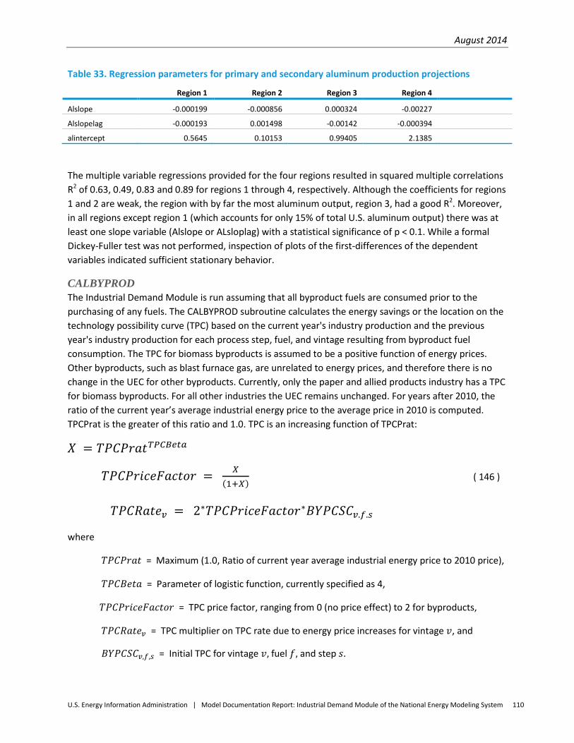
August 2014


Table 33. Regression parameters for primary and secondary aluminum production projections

Region 1 Region 2 Region 3 Region 4

Alslope -0.000199 -0.000856 0.000324 -0.00227

Alslopelag -0.000193 0.001498 -0.00142 -0.000394

alintercept 0.5645 0.10153 0.99405 2.1385

The multiple variable regressions provided for the four regions resulted in squared multiple correlations R2 of 0.63, 0.49, 0.83 and 0.89 for regions 1 through 4, respectively. Although the coefficients for regions 1 and 2 are weak, the region with by far the most aluminum output, region 3, had a good R2. Moreover, in all regions except region 1 (which accounts for only 15% of total U.S. aluminum output) there was at least one slope variable (Alslope or ALsloplag) with a statistical significance of p < 0.1. While a formal Dickey-Fuller test was not performed, inspection of plots of the first-differences of the dependent variables indicated sufficient stationary behavior.

CALBYPROD The Industrial Demand Module is run assuming that all byproduct fuels are consumed prior to the purchasing of any fuels. The CALBYPROD subroutine calculates the energy savings or the location on the technology possibility curve (TPC) based on the current year's industry production and the previous year's industry production for each process step, fuel, and vintage resulting from byproduct fuel consumption. The TPC for biomass byproducts is assumed to be a positive function of energy prices. Other byproducts, such as blast furnace gas, are unrelated to energy prices, and therefore there is no change in the UEC for other byproducts. Currently, only the paper and allied products industry has a TPC for biomass byproducts. For all other industries the UEC remains unchanged. For years after 2010, the ratio of the current year’s average industrial energy price to the average price in 2010 is computed. TPCPrat is the greater of this ratio and 1.0. TPC is an increasing function of TPCPrat:


𝑇𝑃𝐶𝑃𝑟𝑖𝑐𝑒𝐹𝑎𝑐𝑡𝑜𝑟 = 𝑋(1+𝑋)

( 146 )

𝑇𝑃𝐶𝑅𝑎𝑡𝑒𝑣 = 2∗𝑇𝑃𝐶𝑃𝑟𝑖𝑐𝑒𝐹𝑎𝑐𝑡𝑜𝑟∗𝐵𝑌𝑃𝐶𝑆𝐶𝑣.𝑓.𝑠

where

𝑇𝑃𝐶𝑃𝑟𝑎𝑡 = Maximum (1.0, Ratio of current year average industrial energy price to 2010 price),

𝑇𝑃𝐶𝐵𝑒𝑡𝑎 = Parameter of logistic function, currently specified as 4,

𝑇𝑃𝐶𝑃𝑟𝑖𝑐𝑒𝐹𝑎𝑐𝑡𝑜𝑟 = TPC price factor, ranging from 0 (no price effect) to 2 for byproducts,

𝑇𝑃𝐶𝑅𝑎𝑡𝑒𝑣 = TPC multiplier on TPC rate due to energy price increases for vintage 𝑣, and

𝐵𝑌𝑃𝐶𝑆𝐶𝑣,𝑓,𝑠 = Initial TPC for vintage 𝑣, fuel 𝑓, and step 𝑠.

August 2014


CALBYPROD calculates the rate of byproduct energy produced for each process step, fuel, and vintage as shown in the following equation. This value is based on the previous year's rate of production and the current energy savings for each vintage.

𝐵𝑌𝑃𝐼𝑁𝑇𝑣,𝑓,𝑠 = �𝐵𝑌𝑃𝐼𝑁𝑇𝐿𝑎𝑔𝑣,𝑓,𝑠�

𝑇𝑃𝐶𝑅𝑎𝑡𝑒𝑣 (147 )

where

𝐵𝑌𝑃𝐼𝑁𝑇𝑣,𝑓,𝑠 = Rate of byproduct energy production (or UEC) for byproduct fuel 𝑓 at process step 𝑠 for vintage 𝑣,

𝐵𝑌𝑃𝐼𝑁𝑇𝐿𝑎𝑔𝑣,𝑓,𝑠 = Lagged rate of byproduct energy production for byproduct fuel 𝑓 at process step 𝑠 for vintage 𝑣, and

𝑇𝑃𝐶𝑅𝑎𝑡𝑒𝑣 = TPC multiplier on TPC rate due to energy price increases for vintage 𝑣.

The UEC for middle vintage is a weighted average (by production) of the prior year's energy savings for new vintage and the previous year's energy savings for middle vintage.

𝐵𝑌𝑃𝐼𝑁𝑇𝑚𝑖𝑑,𝑓,𝑠 = �

�𝑃𝑅𝑂𝐷𝐿𝑎𝑔𝑚𝑖𝑑,𝑓,𝑠 ∗ 𝐵𝑌𝑃𝐼𝑁𝑇𝐿𝑎𝑔𝑚𝑖𝑑,𝑓,𝑠��𝑃𝑅𝑂𝐷𝐿𝑎𝑔𝑚𝑖𝑑,𝑠 + 𝑃𝑅𝑂𝐷𝐿𝑎𝑔𝑛𝑒𝑤,𝑠�

+

�𝑃𝑅𝑂𝐷𝐿𝑎𝑔𝑛𝑒𝑤,𝑠∗ 𝐵𝑌𝑃𝐼𝑁𝑇𝐿𝑎𝑔𝑛𝑒𝑤,𝑓,𝑠��𝑃𝑅𝑂𝐷𝐿𝑎𝑔𝑚𝑖𝑑,𝑠+ 𝑃𝑅𝑂𝐷𝐿𝑎𝑔𝑛𝑒𝑤,𝑠�

�

𝑇𝑃𝐶𝑅𝑎𝑡𝑒𝑚𝑖𝑑

(148)

where

𝑃𝑅𝑂𝐷𝐿𝑎𝑔𝑛𝑒𝑤,𝑠 = Prior year’s production from new vintage capacity at process step 𝑠,

𝐵𝑌𝑃𝐼𝑁𝑇𝐿𝑎𝑔𝑛𝑒𝑤,𝑓,𝑠 = Lagged rate of byproduct energy production for byproduct fuel 𝑓 at process step 𝑠 for new vintage,

𝑃𝑅𝑂𝐷𝐿𝑎𝑔𝑚𝑖𝑑,𝑠 = Prior year’s production from middle vintage capacity at process step 𝑠,

𝐵𝑌𝑃𝐼𝑁𝑇𝐿𝑎𝑔𝑚𝑖𝑑,𝑓,𝑠 = Lagged rate of byproduct energy production for byproduct fuel 𝑓 at process step 𝑠 for middle vintage, and

𝑇𝑃𝐶𝑅𝑎𝑡𝑒𝑚𝑖𝑑 = TPC multiplier on TPC rate due to energy price increases for middle vintage.

The rate of byproduct fuel production is used to calculate the quantity of byproduct energy produced by multiplying total production at the process step by the production rate.

𝐵𝑌𝑃𝑄𝑇𝑌𝑣,𝑓,𝑠 = 𝑃𝑅𝑂𝐷𝐶𝑈𝑅𝑣,𝑠 ∗ 𝐵𝑌𝑃𝐼𝑁𝑇𝑣,𝑓,𝑠 ( 149 )

where

August 2014


𝐵𝑌𝑃𝑄𝑇𝑌𝑣,𝑓,𝑠 = Byproduct energy production for byproduct fuel 𝑓 at process step 𝑠 for vintage 𝑣,

𝑃𝑅𝑂𝐷𝐶𝑈𝑅𝑣,𝑠 = Production at process step 𝑠 for vintage 𝑣, and

𝐵𝑌𝑃𝐼𝑁𝑇𝑣,𝑓,𝑠 = Rate of byproduct energy production for byproduct fuel 𝑓 at process step 𝑠 for vintage 𝑣.

Note that 𝑃𝑅𝑂𝐷𝐶𝑈𝑅𝑣,𝑠 is production by a vintage at a step and is not fuel-specific. The rate of byproduct fuel production is then converted from millions of Btu to trillions of Btu. Byproduct fuel production is subdivided into three categories: main fuels, intermediate fuels, and renewable fuels.

Byproduct production for each group of fuels is determined by summing byproduct production over the individual process steps for each fuel and vintage as shown below for main byproduct fuels. The equations for intermediate and renewable fuels are similar.

ENBYMf, = ∑ BYPQTYv,f,sMPASTPx=1 (150)

where

𝐸𝑁𝐵𝑌𝑃𝑀𝑓,𝑣 = Byproduct energy production for main byproduct fuel 𝑓 for vintage 𝑣,

𝑀𝑃𝐴𝑆𝑇𝑃 = Number of process steps, and

𝐵𝑌𝑃𝑄𝑇𝑌𝑣,𝑓,𝑠 = Byproduct energy production for byproduct fuel 𝑓 at process step 𝑠 for vintage 𝑣.

CALPATOT CALPATOT calculates the total energy consumption from the process and assembly (PA) component. Energy consumption at each process step is determined by multiplying the current production at that particular process step by the unit energy consumption (UEC) for that process step. Energy consumption is calculated for each fuel, vintage, and step using the following equation.

𝐸𝑁𝑃𝑄𝑇𝑌𝑣,𝑓,𝑠 = 𝑃𝑅𝑂𝐷𝐶𝑈𝑅𝑣,𝑠 ∗ 𝐸𝑁𝑃𝐼𝑁𝑇𝑣,𝑓,𝑠 (151)

where

𝐸𝑁𝑃𝑄𝑇𝑌𝑣,𝑓,𝑠 = Consumption of fuel 𝑓 at process step 𝑠 for vintage 𝑣,

𝑃𝑅𝑂𝐷𝐶𝑈𝑅𝑣,𝑠 = Production at process step 𝑠, for vintage 𝑣, and

𝐸𝑁𝑃𝐼𝑁𝑇𝑣,𝑓,𝑠 = Unit energy consumption of fuel 𝑓 at process step 𝑠 for vintage 𝑣.

Consumption of each fuel is converted to trillions of Btu. Energy consumption is subdivided into main fuels, intermediate fuels, and renewable fuels. The main fuel group includes:40

40Still gas and petroleum coke are consumed primarily in the refining industry, which is modeled in the Liquid Fuels Market Module of NEMS.

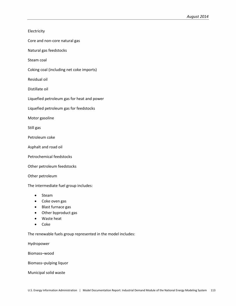
August 2014


Electricity

Core and non-core natural gas

Natural gas feedstocks

Steam coal

Coking coal (including net coke imports)

Residual oil

Distillate oil

Liquefied petroleum gas for heat and power

Liquefied petroleum gas for feedstocks

Motor gasoline

Still gas

Petroleum coke

Asphalt and road oil

Petrochemical feedstocks

Other petroleum feedstocks

Other petroleum

The intermediate fuel group includes:

• Steam • Coke oven gas • Blast furnace gas • Other byproduct gas • Waste heat • Coke

The renewable fuels group represented in the model includes:

Hydropower

Biomass–wood

Biomass–pulping liquor

Municipal solid waste

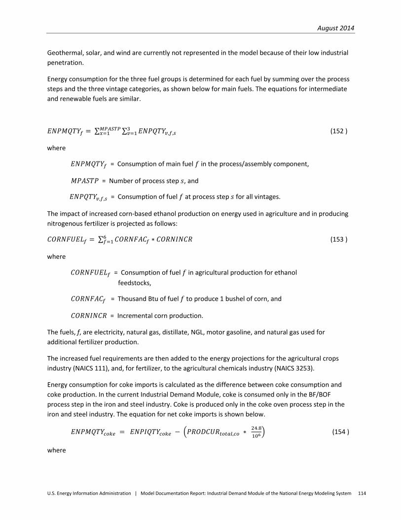
August 2014


Geothermal, solar, and wind are currently not represented in the model because of their low industrial penetration.

Energy consumption for the three fuel groups is determined for each fuel by summing over the process steps and the three vintage categories, as shown below for main fuels. The equations for intermediate and renewable fuels are similar.

𝐸𝑁𝑃𝑀𝑄𝑇𝑌𝑓 = ∑ ∑ 𝐸𝑁𝑃𝑄𝑇𝑌𝑣,𝑓,𝑠3𝑣=1

𝑀𝑃𝐴𝑆𝑇𝑃𝑥=1 (152 )

where

𝐸𝑁𝑃𝑀𝑄𝑇𝑌𝑓 = Consumption of main fuel 𝑓 in the process/assembly component,

𝑀𝑃𝐴𝑆𝑇𝑃 = Number of process step 𝑠, and

𝐸𝑁𝑃𝑄𝑇𝑌𝑣,𝑓,𝑠 = Consumption of fuel 𝑓 at process step 𝑠 for all vintages.

The impact of increased corn-based ethanol production on energy used in agriculture and in producing nitrogenous fertilizer is projected as follows:

𝐶𝑂𝑅𝑁𝐹𝑈𝐸𝐿𝑓 = ∑ 𝐶𝑂𝑅𝑁𝐹𝐴𝐶𝑓6𝑓=1 ∗ 𝐶𝑂𝑅𝑁𝐼𝑁𝐶𝑅 (153 )

where

𝐶𝑂𝑅𝑁𝐹𝑈𝐸𝐿𝑓 = Consumption of fuel 𝑓 in agricultural production for ethanol feedstocks,

𝐶𝑂𝑅𝑁𝐹𝐴𝐶𝑓 = Thousand Btu of fuel 𝑓 to produce 1 bushel of corn, and

𝐶𝑂𝑅𝑁𝐼𝑁𝐶𝑅 = Incremental corn production.

The fuels, f, are electricity, natural gas, distillate, NGL, motor gasoline, and natural gas used for additional fertilizer production.

The increased fuel requirements are then added to the energy projections for the agricultural crops industry (NAICS 111), and, for fertilizer, to the agricultural chemicals industry (NAICS 3253).

Energy consumption for coke imports is calculated as the difference between coke consumption and coke production. In the current Industrial Demand Module, coke is consumed only in the BF/BOF process step in the iron and steel industry. Coke is produced only in the coke oven process step in the iron and steel industry. The equation for net coke imports is shown below.

𝐸𝑁𝑃𝑀𝑄𝑇𝑌𝑐𝑜𝑘𝑒 = 𝐸𝑁𝑃𝐼𝑄𝑇𝑌𝑐𝑜𝑘𝑒 − �𝑃𝑅𝑂𝐷𝐶𝑈𝑅𝑡𝑜𝑡𝑎𝑙,𝑐𝑜 ∗ 24.8106

� (154 )

where

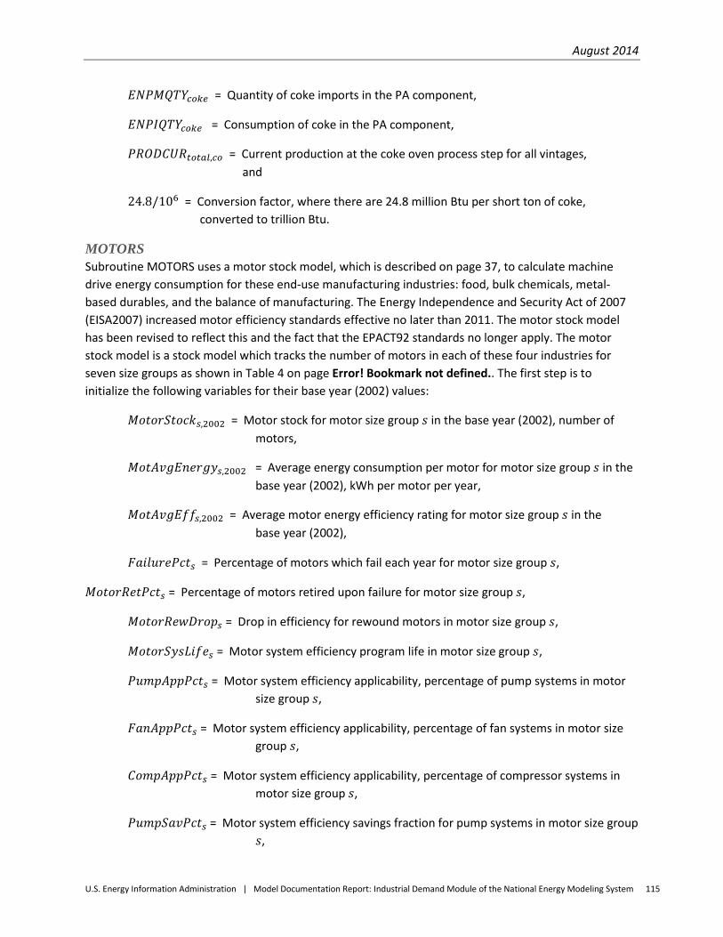
August 2014


𝐸𝑁𝑃𝑀𝑄𝑇𝑌𝑐𝑜𝑘𝑒 = Quantity of coke imports in the PA component,

𝐸𝑁𝑃𝐼𝑄𝑇𝑌𝑐𝑜𝑘𝑒 = Consumption of coke in the PA component,

𝑃𝑅𝑂𝐷𝐶𝑈𝑅𝑡𝑜𝑡𝑎𝑙,𝑐𝑜 = Current production at the coke oven process step for all vintages, and

24.8/106 = Conversion factor, where there are 24.8 million Btu per short ton of coke, converted to trillion Btu.

MOTORS Subroutine MOTORS uses a motor stock model, which is described on page 37, to calculate machine drive energy consumption for these end-use manufacturing industries: food, bulk chemicals, metal-based durables, and the balance of manufacturing. The Energy Independence and Security Act of 2007 (EISA2007) increased motor efficiency standards effective no later than 2011. The motor stock model has been revised to reflect this and the fact that the EPACT92 standards no longer apply. The motor stock model is a stock model which tracks the number of motors in each of these four industries for seven size groups as shown in Table 4 on page Error! Bookmark not defined.. The first step is to initialize the following variables for their base year (2002) values:

𝑀𝑜𝑡𝑜𝑟𝑆𝑡𝑜𝑐𝑘𝑠,2002 = Motor stock for motor size group 𝑠 in the base year (2002), number of motors,

𝑀𝑜𝑡𝐴𝑣𝑔𝐸𝑛𝑒𝑟𝑔𝑦𝑠,2002 = Average energy consumption per motor for motor size group 𝑠 in the base year (2002), kWh per motor per year,

𝑀𝑜𝑡𝐴𝑣𝑔𝐸𝑓𝑓𝑠,2002 = Average motor energy efficiency rating for motor size group 𝑠 in the base year (2002),

𝐹𝑎𝑖𝑙𝑢𝑟𝑒𝑃𝑐𝑡𝑠 = Percentage of motors which fail each year for motor size group 𝑠,

𝑀𝑜𝑡𝑜𝑟𝑅𝑒𝑡𝑃𝑐𝑡𝑠 = Percentage of motors retired upon failure for motor size group 𝑠,

𝑀𝑜𝑡𝑜𝑟𝑅𝑒𝑤𝐷𝑟𝑜𝑝𝑠 = Drop in efficiency for rewound motors in motor size group 𝑠,

𝑀𝑜𝑡𝑜𝑟𝑆𝑦𝑠𝐿𝑖𝑓𝑒𝑠 = Motor system efficiency program life in motor size group 𝑠,

𝑃𝑢𝑚𝑝𝐴𝑝𝑝𝑃𝑐𝑡𝑠 = Motor system efficiency applicability, percentage of pump systems in motor size group 𝑠,

𝐹𝑎𝑛𝐴𝑝𝑝𝑃𝑐𝑡𝑠 = Motor system efficiency applicability, percentage of fan systems in motor size group 𝑠,

𝐶𝑜𝑚𝑝𝐴𝑝𝑝𝑃𝑐𝑡𝑠 = Motor system efficiency applicability, percentage of compressor systems in motor size group 𝑠,

𝑃𝑢𝑚𝑝𝑆𝑎𝑣𝑃𝑐𝑡𝑠 = Motor system efficiency savings fraction for pump systems in motor size group 𝑠,

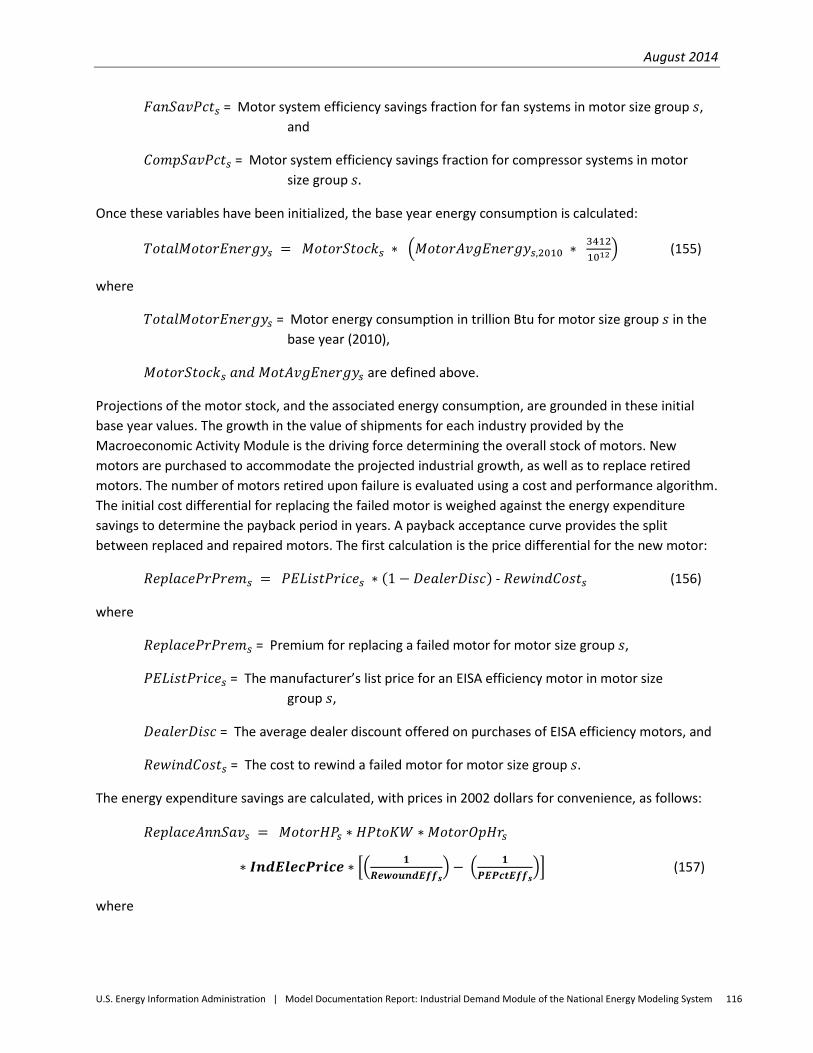
August 2014


𝐹𝑎𝑛𝑆𝑎𝑣𝑃𝑐𝑡𝑠 = Motor system efficiency savings fraction for fan systems in motor size group 𝑠, and

𝐶𝑜𝑚𝑝𝑆𝑎𝑣𝑃𝑐𝑡𝑠 = Motor system efficiency savings fraction for compressor systems in motor size group 𝑠.

Once these variables have been initialized, the base year energy consumption is calculated:

𝑇𝑜𝑡𝑎𝑙𝑀𝑜𝑡𝑜𝑟𝐸𝑛𝑒𝑟𝑔𝑦𝑠 = 𝑀𝑜𝑡𝑜𝑟𝑆𝑡𝑜𝑐𝑘𝑠 ∗ �𝑀𝑜𝑡𝑜𝑟𝐴𝑣𝑔𝐸𝑛𝑒𝑟𝑔𝑦𝑠,2010 ∗ 34121012

� (155)

where

𝑇𝑜𝑡𝑎𝑙𝑀𝑜𝑡𝑜𝑟𝐸𝑛𝑒𝑟𝑔𝑦𝑠 = Motor energy consumption in trillion Btu for motor size group 𝑠 in the base year (2010),

𝑀𝑜𝑡𝑜𝑟𝑆𝑡𝑜𝑐𝑘𝑠 𝑎𝑛𝑑 𝑀𝑜𝑡𝐴𝑣𝑔𝐸𝑛𝑒𝑟𝑔𝑦𝑠 are defined above.

Projections of the motor stock, and the associated energy consumption, are grounded in these initial base year values. The growth in the value of shipments for each industry provided by the Macroeconomic Activity Module is the driving force determining the overall stock of motors. New motors are purchased to accommodate the projected industrial growth, as well as to replace retired motors. The number of motors retired upon failure is evaluated using a cost and performance algorithm. The initial cost differential for replacing the failed motor is weighed against the energy expenditure savings to determine the payback period in years. A payback acceptance curve provides the split between replaced and repaired motors. The first calculation is the price differential for the new motor:

𝑅𝑒𝑝𝑙𝑎𝑐𝑒𝑃𝑟𝑃𝑟𝑒𝑚𝑠 = 𝑃𝐸𝐿𝑖𝑠𝑡𝑃𝑟𝑖𝑐𝑒𝑠 ∗ (1 − 𝐷𝑒𝑎𝑙𝑒𝑟𝐷𝑖𝑠𝑐) - 𝑅𝑒𝑤𝑖𝑛𝑑𝐶𝑜𝑠𝑡𝑠 (156)

where

𝑅𝑒𝑝𝑙𝑎𝑐𝑒𝑃𝑟𝑃𝑟𝑒𝑚𝑠 = Premium for replacing a failed motor for motor size group 𝑠,

𝑃𝐸𝐿𝑖𝑠𝑡𝑃𝑟𝑖𝑐𝑒𝑠 = The manufacturer’s list price for an EISA efficiency motor in motor size group 𝑠,

𝐷𝑒𝑎𝑙𝑒𝑟𝐷𝑖𝑠𝑐 = The average dealer discount offered on purchases of EISA efficiency motors, and

𝑅𝑒𝑤𝑖𝑛𝑑𝐶𝑜𝑠𝑡𝑠 = The cost to rewind a failed motor for motor size group 𝑠.

The energy expenditure savings are calculated, with prices in 2002 dollars for convenience, as follows:

𝑅𝑒𝑝𝑙𝑎𝑐𝑒𝐴𝑛𝑛𝑆𝑎𝑣𝑠 = 𝑀𝑜𝑡𝑜𝑟𝐻𝑃𝑠 ∗ 𝐻𝑃𝑡𝑜𝐾𝑊 ∗𝑀𝑜𝑡𝑜𝑟𝑂𝑝𝐻𝑟𝑠

∗ 𝑰𝒏𝒅𝑬𝒍𝒆𝒄𝑷𝒓𝒊𝒄𝒆 ∗ �� 𝟏𝑹𝒆𝒘𝒐𝒖𝒏𝒅𝑬𝒇𝒇𝒔

� − � 𝟏𝑷𝑬𝑷𝒄𝒕𝑬𝒇𝒇𝒔

�� (157)

where

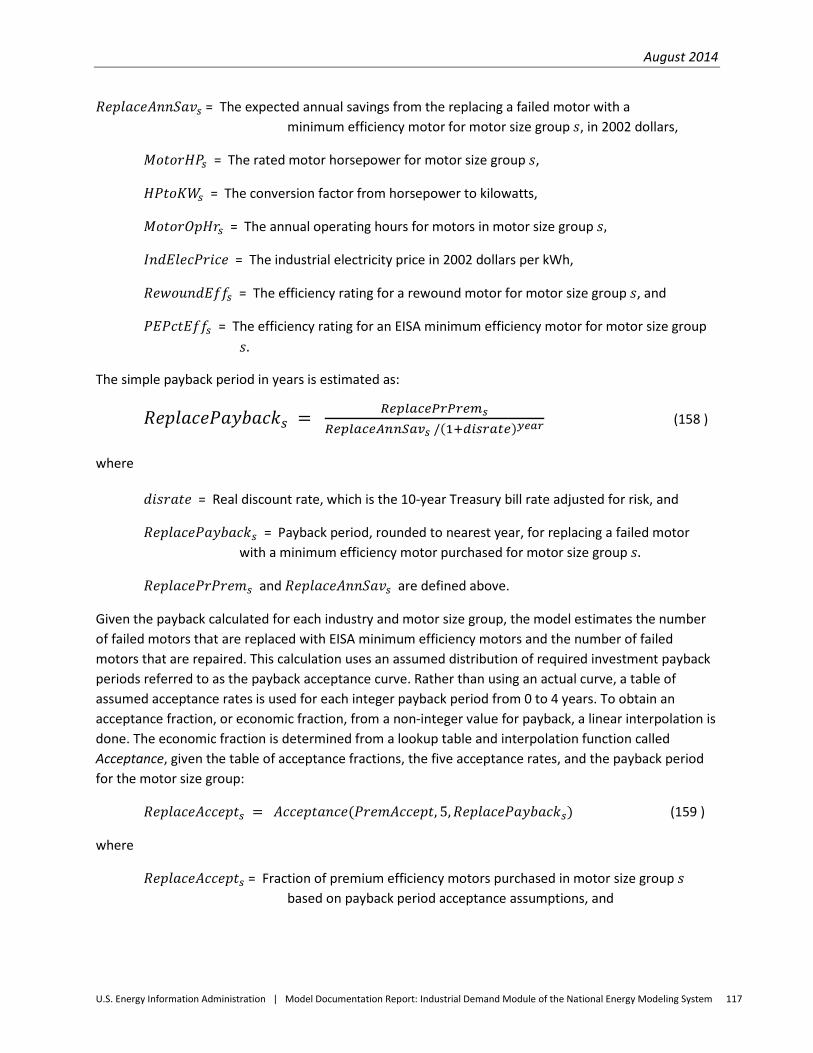
August 2014


𝑅𝑒𝑝𝑙𝑎𝑐𝑒𝐴𝑛𝑛𝑆𝑎𝑣𝑠 = The expected annual savings from the replacing a failed motor with a minimum efficiency motor for motor size group 𝑠, in 2002 dollars,

𝑀𝑜𝑡𝑜𝑟𝐻𝑃𝑠 = The rated motor horsepower for motor size group 𝑠,

𝐻𝑃𝑡𝑜𝐾𝑊𝑠 = The conversion factor from horsepower to kilowatts,

𝑀𝑜𝑡𝑜𝑟𝑂𝑝𝐻𝑟𝑠 = The annual operating hours for motors in motor size group 𝑠,

𝐼𝑛𝑑𝐸𝑙𝑒𝑐𝑃𝑟𝑖𝑐𝑒 = The industrial electricity price in 2002 dollars per kWh,

𝑅𝑒𝑤𝑜𝑢𝑛𝑑𝐸𝑓𝑓𝑠 = The efficiency rating for a rewound motor for motor size group 𝑠, and

𝑃𝐸𝑃𝑐𝑡𝐸𝑓𝑓𝑠 = The efficiency rating for an EISA minimum efficiency motor for motor size group 𝑠.

The simple payback period in years is estimated as:

𝑅𝑒𝑝𝑙𝑎𝑐𝑒𝑃𝑎𝑦𝑏𝑎𝑐𝑘𝑠 = 𝑅𝑒𝑝𝑙𝑎𝑐𝑒𝑃𝑟𝑃𝑟𝑒𝑚𝑠𝑅𝑒𝑝𝑙𝑎𝑐𝑒𝐴𝑛𝑛𝑆𝑎𝑣𝑠 /(1+𝑑𝑖𝑠𝑟𝑎𝑡𝑒)𝑦𝑒𝑎𝑟

(158 )

where

𝑑𝑖𝑠𝑟𝑎𝑡𝑒 = Real discount rate, which is the 10-year Treasury bill rate adjusted for risk, and

𝑅𝑒𝑝𝑙𝑎𝑐𝑒𝑃𝑎𝑦𝑏𝑎𝑐𝑘𝑠 = Payback period, rounded to nearest year, for replacing a failed motor with a minimum efficiency motor purchased for motor size group 𝑠.

𝑅𝑒𝑝𝑙𝑎𝑐𝑒𝑃𝑟𝑃𝑟𝑒𝑚𝑠 and 𝑅𝑒𝑝𝑙𝑎𝑐𝑒𝐴𝑛𝑛𝑆𝑎𝑣𝑠 are defined above.

Given the payback calculated for each industry and motor size group, the model estimates the number of failed motors that are replaced with EISA minimum efficiency motors and the number of failed motors that are repaired. This calculation uses an assumed distribution of required investment payback periods referred to as the payback acceptance curve. Rather than using an actual curve, a table of assumed acceptance rates is used for each integer payback period from 0 to 4 years. To obtain an acceptance fraction, or economic fraction, from a non-integer value for payback, a linear interpolation is done. The economic fraction is determined from a lookup table and interpolation function called Acceptance, given the table of acceptance fractions, the five acceptance rates, and the payback period for the motor size group:

𝑅𝑒𝑝𝑙𝑎𝑐𝑒𝐴𝑐𝑐𝑒𝑝𝑡𝑠 = 𝐴𝑐𝑐𝑒𝑝𝑡𝑎𝑛𝑐𝑒(𝑃𝑟𝑒𝑚𝐴𝑐𝑐𝑒𝑝𝑡, 5,𝑅𝑒𝑝𝑙𝑎𝑐𝑒𝑃𝑎𝑦𝑏𝑎𝑐𝑘𝑠) (159 )

where

𝑅𝑒𝑝𝑙𝑎𝑐𝑒𝐴𝑐𝑐𝑒𝑝𝑡𝑠 = Fraction of premium efficiency motors purchased in motor size group 𝑠 based on payback period acceptance assumptions, and

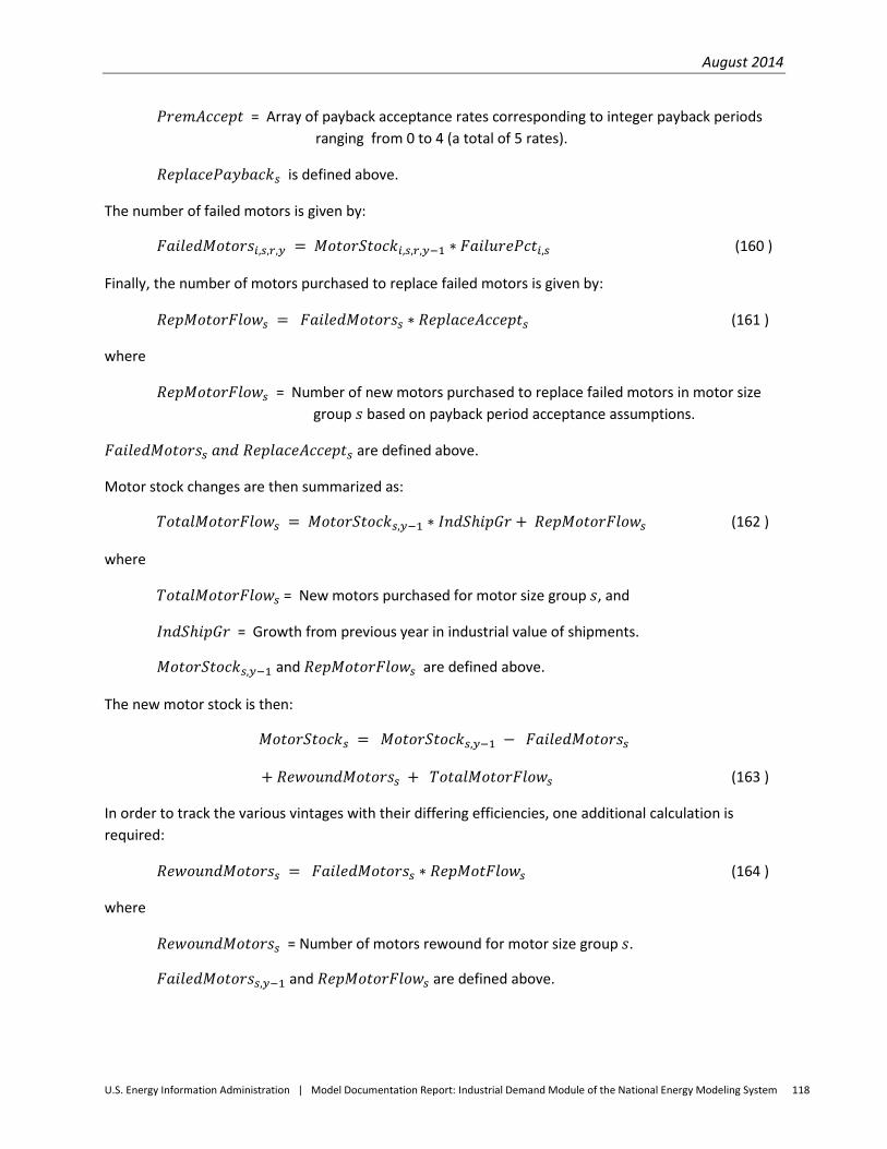
August 2014


𝑃𝑟𝑒𝑚𝐴𝑐𝑐𝑒𝑝𝑡 = Array of payback acceptance rates corresponding to integer payback periods ranging from 0 to 4 (a total of 5 rates).

𝑅𝑒𝑝𝑙𝑎𝑐𝑒𝑃𝑎𝑦𝑏𝑎𝑐𝑘𝑠 is defined above.

The number of failed motors is given by:

𝐹𝑎𝑖𝑙𝑒𝑑𝑀𝑜𝑡𝑜𝑟𝑠𝑖,𝑠,𝑟,𝑦 = 𝑀𝑜𝑡𝑜𝑟𝑆𝑡𝑜𝑐𝑘𝑖,𝑠,𝑟,𝑦−1 ∗ 𝐹𝑎𝑖𝑙𝑢𝑟𝑒𝑃𝑐𝑡𝑖,𝑠 (160 )

Finally, the number of motors purchased to replace failed motors is given by:

𝑅𝑒𝑝𝑀𝑜𝑡𝑜𝑟𝐹𝑙𝑜𝑤𝑠 = 𝐹𝑎𝑖𝑙𝑒𝑑𝑀𝑜𝑡𝑜𝑟𝑠𝑠 ∗ 𝑅𝑒𝑝𝑙𝑎𝑐𝑒𝐴𝑐𝑐𝑒𝑝𝑡𝑠 (161 )

where

𝑅𝑒𝑝𝑀𝑜𝑡𝑜𝑟𝐹𝑙𝑜𝑤𝑠 = Number of new motors purchased to replace failed motors in motor size group 𝑠 based on payback period acceptance assumptions.

𝐹𝑎𝑖𝑙𝑒𝑑𝑀𝑜𝑡𝑜𝑟𝑠𝑠 𝑎𝑛𝑑 𝑅𝑒𝑝𝑙𝑎𝑐𝑒𝐴𝑐𝑐𝑒𝑝𝑡𝑠 are defined above.

Motor stock changes are then summarized as:

𝑇𝑜𝑡𝑎𝑙𝑀𝑜𝑡𝑜𝑟𝐹𝑙𝑜𝑤𝑠 = 𝑀𝑜𝑡𝑜𝑟𝑆𝑡𝑜𝑐𝑘𝑠,𝑦−1 ∗ 𝐼𝑛𝑑𝑆ℎ𝑖𝑝𝐺𝑟 + 𝑅𝑒𝑝𝑀𝑜𝑡𝑜𝑟𝐹𝑙𝑜𝑤𝑠 (162 )

where

𝑇𝑜𝑡𝑎𝑙𝑀𝑜𝑡𝑜𝑟𝐹𝑙𝑜𝑤𝑠 = New motors purchased for motor size group 𝑠, and

𝐼𝑛𝑑𝑆ℎ𝑖𝑝𝐺𝑟 = Growth from previous year in industrial value of shipments.

𝑀𝑜𝑡𝑜𝑟𝑆𝑡𝑜𝑐𝑘𝑠,𝑦−1 and 𝑅𝑒𝑝𝑀𝑜𝑡𝑜𝑟𝐹𝑙𝑜𝑤𝑠 are defined above.

The new motor stock is then:

𝑀𝑜𝑡𝑜𝑟𝑆𝑡𝑜𝑐𝑘𝑠 = 𝑀𝑜𝑡𝑜𝑟𝑆𝑡𝑜𝑐𝑘𝑠,𝑦−1 − 𝐹𝑎𝑖𝑙𝑒𝑑𝑀𝑜𝑡𝑜𝑟𝑠𝑠

+ 𝑅𝑒𝑤𝑜𝑢𝑛𝑑𝑀𝑜𝑡𝑜𝑟𝑠𝑠 + 𝑇𝑜𝑡𝑎𝑙𝑀𝑜𝑡𝑜𝑟𝐹𝑙𝑜𝑤𝑠 (163 )

In order to track the various vintages with their differing efficiencies, one additional calculation is required:

𝑅𝑒𝑤𝑜𝑢𝑛𝑑𝑀𝑜𝑡𝑜𝑟𝑠𝑠 = 𝐹𝑎𝑖𝑙𝑒𝑑𝑀𝑜𝑡𝑜𝑟𝑠𝑠 ∗ 𝑅𝑒𝑝𝑀𝑜𝑡𝐹𝑙𝑜𝑤𝑠 (164 )

where

𝑅𝑒𝑤𝑜𝑢𝑛𝑑𝑀𝑜𝑡𝑜𝑟𝑠𝑠 = Number of motors rewound for motor size group 𝑠.

𝐹𝑎𝑖𝑙𝑒𝑑𝑀𝑜𝑡𝑜𝑟𝑠𝑠,𝑦−1 and 𝑅𝑒𝑝𝑀𝑜𝑡𝑜𝑟𝐹𝑙𝑜𝑤𝑠 are defined above.

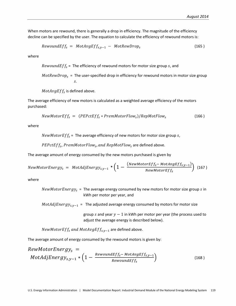
August 2014


When motors are rewound, there is generally a drop in efficiency. The magnitude of the efficiency decline can be specified by the user. The equation to calculate the efficiency of rewound motors is:

𝑅𝑒𝑤𝑜𝑢𝑛𝑑𝐸𝑓𝑓𝑠 = 𝑀𝑜𝑡𝐴𝑣𝑔𝐸𝑓𝑓𝑠,𝑦−1 − 𝑀𝑜𝑡𝑅𝑒𝑤𝐷𝑟𝑜𝑝𝑠 (165 )

where

𝑅𝑒𝑤𝑜𝑢𝑛𝑑𝐸𝑓𝑓𝑠 = The efficiency of rewound motors for motor size group 𝑠, and

𝑀𝑜𝑡𝑅𝑒𝑤𝐷𝑟𝑜𝑝𝑠 = The user-specified drop in efficiency for rewound motors in motor size group 𝑠.

𝑀𝑜𝑡𝐴𝑣𝑔𝐸𝑓𝑓𝑠 is defined above.

The average efficiency of new motors is calculated as a weighted average efficiency of the motors purchased:

𝑁𝑒𝑤𝑀𝑜𝑡𝑜𝑟𝐸𝑓𝑓𝑠 = (𝑃𝐸𝑃𝑐𝑡𝐸𝑓𝑓𝑠 ∗ 𝑃𝑟𝑒𝑚𝑀𝑜𝑡𝑜𝑟𝐹𝑙𝑜𝑤𝑠)/𝑅𝑒𝑝𝑀𝑜𝑡𝐹𝑙𝑜𝑤𝑠 (166 )

where

𝑁𝑒𝑤𝑀𝑜𝑡𝑜𝑟𝐸𝑓𝑓𝑠 = The average efficiency of new motors for motor size group 𝑠,

𝑃𝐸𝑃𝑐𝑡𝐸𝑓𝑓𝑠, 𝑃𝑟𝑒𝑚𝑀𝑜𝑡𝑜𝑟𝐹𝑙𝑜𝑤𝑠,𝑎𝑛𝑑 𝑅𝑒𝑝𝑀𝑜𝑡𝐹𝑙𝑜𝑤𝑠 are defined above.

The average amount of energy consumed by the new motors purchased is given by

𝑁𝑒𝑤𝑀𝑜𝑡𝑜𝑟𝐸𝑛𝑒𝑟𝑔𝑦𝑠 = 𝑀𝑜𝑡𝐴𝑑𝑗𝐸𝑛𝑒𝑟𝑔𝑦𝑠,𝑦−1 * �1 − �𝑁𝑒𝑤𝑀𝑜𝑡𝑜𝑟𝐸𝑓𝑓𝑠− 𝑀𝑜𝑡𝐴𝑣𝑔𝐸𝑓𝑓𝑠,𝑦−1�𝑁𝑒𝑤𝑀𝑜𝑡𝑜𝑟𝐸𝑓𝑓𝑠

� (167 )

where

𝑁𝑒𝑤𝑀𝑜𝑡𝑜𝑟𝐸𝑛𝑒𝑟𝑔𝑦𝑠 = The average energy consumed by new motors for motor size group 𝑠 in kWh per motor per year, and

𝑀𝑜𝑡𝐴𝑑𝑗𝐸𝑛𝑒𝑟𝑔𝑦𝑠,𝑦−1 = The adjusted average energy consumed by motors for motor size

group 𝑠 and year 𝑦 − 1 in kWh per motor per year (the process used to adjust the average energy is described below).

𝑁𝑒𝑤𝑀𝑜𝑡𝑜𝑟𝐸𝑓𝑓𝑠 𝑎𝑛𝑑 𝑀𝑜𝑡𝐴𝑣𝑔𝐸𝑓𝑓𝑠,𝑦−1 are defined above.

The average amount of energy consumed by the rewound motors is given by:

𝑅𝑒𝑤𝑀𝑜𝑡𝑜𝑟𝐸𝑛𝑒𝑟𝑔𝑦𝑠 = 𝑀𝑜𝑡𝐴𝑑𝑗𝐸𝑛𝑒𝑟𝑔𝑦𝑠,𝑦−1 ∗ �1 − 𝑅𝑒𝑤𝑜𝑢𝑛𝑑𝐸𝑓𝑓𝑠− 𝑀𝑜𝑡𝐴𝑣𝑔𝐸𝑓𝑓𝑠,𝑦−1

𝑅𝑒𝑤𝑜𝑢𝑛𝑑𝐸𝑓𝑓𝑠� (168 )

August 2014


where

𝑅𝑒𝑤𝑀𝑜𝑡𝑜𝑟𝐸𝑛𝑒𝑟𝑔𝑦𝑠 = The average energy consumed by rewound motors for motor size group 𝑠 in kWh per motor per year, and

𝑀𝑜𝑡𝐴𝑑𝑗𝐸𝑛𝑒𝑟𝑔𝑦𝑠,𝑦−1 = The adjusted average energy consumed by motors for motor size group 𝑠 and year 𝑦 − 1 in kWh per motor per year (the process used to adjust the average energy is described below).

𝑅𝑒𝑤𝑜𝑢𝑛𝑑𝐸𝑓𝑓𝑠 𝑎𝑛𝑑 𝑀𝑜𝑡𝐴𝑣𝑔𝐸𝑓𝑓𝑠,𝑦−1 are defined above.

The average amount of energy consumed by all motors in the stock is given by:

𝑀𝑜𝑡𝐴𝑣𝑔𝐸𝑛𝑒𝑟𝑔𝑦𝑠 = ⎝⎜⎛

𝑀𝑜𝑡𝐴𝑑𝑗𝐸𝑛𝑒𝑟𝑔𝑦𝑠,𝑦−1∗�𝑀𝑜𝑡𝑜𝑟𝑆𝑡𝑜𝑐𝑘𝑠,𝑦−1 − 𝐹𝑎𝑖𝑙𝑒𝑑𝑀𝑜𝑡𝑜𝑟𝑠𝑠�

+ (𝑇𝑜𝑡𝑎𝑙𝑀𝑜𝑡𝑜𝑟𝐹𝑙𝑜𝑤𝑠∗𝑁𝑒𝑤𝑀𝑜𝑡𝑜𝑟𝐸𝑛𝑒𝑟𝑔𝑦𝑠)+ (𝑅𝑒𝑤𝑜𝑢𝑛𝑑𝑀𝑜𝑡𝑜𝑟𝑠𝑠∗𝑅𝑒𝑤𝑀𝑜𝑡𝑜𝑟𝐸𝑛𝑒𝑟𝑔𝑦𝑠)⎠

⎟⎞

𝑀𝑜𝑡𝑜𝑟𝑆𝑡𝑜𝑐𝑘𝑠 (169 )

where

𝑀𝑜𝑡𝐴𝑣𝑔𝐸𝑛𝑒𝑟𝑔𝑦𝑠 = The average energy consumed by all motors for motor size group 𝑠 in kWh per motor per year, and

𝑀𝑜𝑡𝐴𝑑𝑗𝐸𝑛𝑒𝑟𝑔𝑦𝑠,𝑦−1 = The adjusted average energy consumed by motors for motor size group 𝑠 and year 𝑦 − 1 in kWh per motor per year (the process used to adjust the average energy is described below).

𝑀𝑜𝑡𝑜𝑟𝑆𝑡𝑜𝑐𝑘𝑠,𝑦−1,𝐹𝑎𝑖𝑙𝑒𝑑𝑀𝑜𝑡𝑜𝑟𝑠𝑠,𝑇𝑜𝑡𝑎𝑙𝑀𝑜𝑡𝑜𝑟𝐹𝑙𝑜𝑤𝑠,𝑁𝑒𝑤𝑀𝑜𝑡𝑜𝑟𝐸𝑛𝑒𝑟𝑔𝑦𝑠,𝑅𝑒𝑤𝑜𝑢𝑛𝑑𝑀𝑜𝑡𝑜𝑟𝑠𝑠, 𝑅𝑒𝑤𝑀𝑜𝑡𝑜𝑟𝐸𝑛𝑒𝑟𝑔𝑦𝑠, and 𝑀𝑜𝑡𝐴𝑑𝑗𝐸𝑛𝑒𝑟𝑔𝑦𝑠,𝑦−1 are defined above.

The average energy efficiency of the stock of motors is given by:

𝑅𝑒𝑤𝑜𝑢𝑛𝑑𝐸𝑓𝑓𝑠 = 𝑀𝑜𝑡𝐴𝑣𝑔𝐸𝑓𝑓𝑠,𝑦−1 − 𝑀𝑜𝑡𝑅𝑒𝑤𝐷𝑟𝑜𝑝𝑠 (170 )

where

𝑀𝑜𝑡𝐴𝑣𝑔𝐸𝑓𝑓𝑠 = The average energy efficiency of motors for motor size group 𝑠

𝑅𝑒𝑤𝑜𝑢𝑛𝑑𝐸𝑓𝑓𝑠 and 𝑀𝑜𝑡𝑅𝑒𝑤𝐷𝑟𝑜𝑝𝑠 are defined above.

The energy efficiency of motor systems is affected not only by the efficiency of the motors themselves, but also by the efficiency of the systems in which the motors are used. The three largest categories of motor systems are pump systems, fan systems, and compressor systems. The following equation calculates the overall motor system energy consumption savings rate:

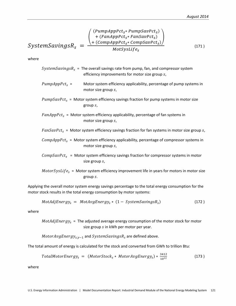
August 2014


𝑆𝑦𝑠𝑡𝑒𝑚𝑆𝑎𝑣𝑖𝑛𝑔𝑠𝑅𝑠 = �

(𝑃𝑢𝑚𝑝𝐴𝑝𝑝𝑃𝑐𝑡𝑠∗ 𝑃𝑢𝑚𝑝𝑆𝑎𝑣𝑃𝑐𝑡𝑠)+ (𝐹𝑎𝑛𝐴𝑝𝑝𝑃𝑐𝑡𝑠∗ 𝐹𝑎𝑛𝑆𝑎𝑣𝑃𝑐𝑡𝑠)

+ (𝐶𝑜𝑚𝑝𝐴𝑝𝑝𝑃𝑐𝑡𝑠∗ 𝐶𝑜𝑚𝑝𝑆𝑎𝑣𝑃𝑐𝑡𝑠)�

𝑀𝑜𝑡𝑆𝑦𝑠𝐿𝑖𝑓𝑒𝑠 (171 )

where

𝑆𝑦𝑠𝑡𝑒𝑚𝑆𝑎𝑣𝑖𝑛𝑔𝑠𝑅𝑠 = The overall savings rate from pump, fan, and compressor system efficiency improvements for motor size group 𝑠,

𝑃𝑢𝑚𝑝𝐴𝑝𝑝𝑃𝑐𝑡𝑠 = Motor system efficiency applicability, percentage of pump systems in motor size group 𝑠,

𝑃𝑢𝑚𝑝𝑆𝑎𝑣𝑃𝑐𝑡𝑠 = Motor system efficiency savings fraction for pump systems in motor size group 𝑠,

𝐹𝑎𝑛𝐴𝑝𝑝𝑃𝑐𝑡𝑠 = Motor system efficiency applicability, percentage of fan systems in motor size group 𝑠,

𝐹𝑎𝑛𝑆𝑎𝑣𝑃𝑐𝑡𝑠 = Motor system efficiency savings fraction for fan systems in motor size group 𝑠,

𝐶𝑜𝑚𝑝𝐴𝑝𝑝𝑃𝑐𝑡𝑠 = Motor system efficiency applicability, percentage of compressor systems in motor size group 𝑠,

𝐶𝑜𝑚𝑝𝑆𝑎𝑣𝑃𝑐𝑡𝑠 = Motor system efficiency savings fraction for compressor systems in motor size group 𝑠,

𝑀𝑜𝑡𝑜𝑟𝑆𝑦𝑠𝐿𝑖𝑓𝑒𝑠 = Motor system efficiency improvement life in years for motors in motor size group 𝑠.

Applying the overall motor system energy savings percentage to the total energy consumption for the motor stock results in the total energy consumption by motor systems:

𝑀𝑜𝑡𝐴𝑑𝑗𝐸𝑛𝑒𝑟𝑔𝑦𝑠 = 𝑀𝑜𝑡𝐴𝑣𝑔𝐸𝑛𝑒𝑟𝑔𝑦𝑠 ∗ (1 − 𝑆𝑦𝑠𝑡𝑒𝑚𝑆𝑎𝑣𝑖𝑛𝑔𝑠𝑅𝑠) (172 )

where

𝑀𝑜𝑡𝐴𝑑𝑗𝐸𝑛𝑒𝑟𝑔𝑦𝑠 = The adjusted average energy consumption of the motor stock for motor size group 𝑠 in kWh per motor per year.

𝑀𝑜𝑡𝑜𝑟𝐴𝑣𝑔𝐸𝑛𝑒𝑟𝑔𝑦𝑠,𝑦−1 and 𝑆𝑦𝑠𝑡𝑒𝑚𝑆𝑎𝑣𝑖𝑛𝑔𝑠𝑅𝑠 are defined above.

The total amount of energy is calculated for the stock and converted from GWh to trillion Btu:

𝑇𝑜𝑡𝑎𝑙𝑀𝑜𝑡𝑜𝑟𝐸𝑛𝑒𝑟𝑔𝑦𝑠 = (𝑀𝑜𝑡𝑜𝑟𝑆𝑡𝑜𝑐𝑘𝑠 ∗ 𝑀𝑜𝑡𝑜𝑟𝐴𝑣𝑔𝐸𝑛𝑒𝑟𝑔𝑦𝑠) ∗ 34121012

(173 )

where

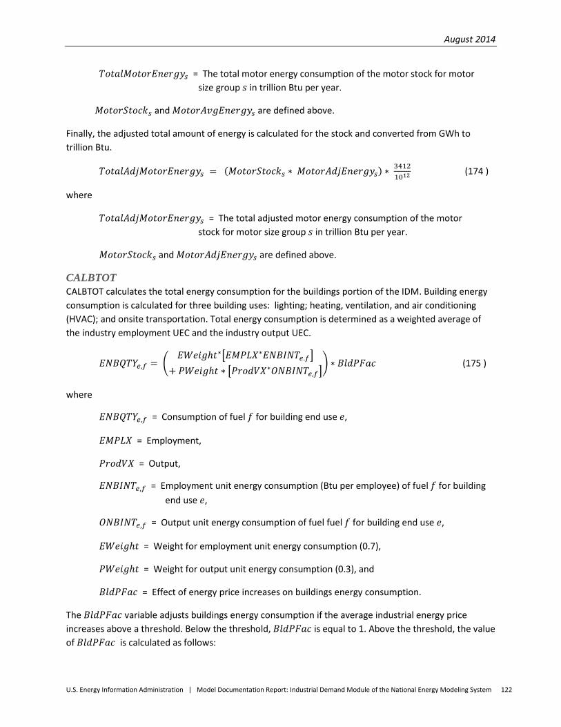
August 2014


𝑇𝑜𝑡𝑎𝑙𝑀𝑜𝑡𝑜𝑟𝐸𝑛𝑒𝑟𝑔𝑦𝑠 = The total motor energy consumption of the motor stock for motor size group 𝑠 in trillion Btu per year.

𝑀𝑜𝑡𝑜𝑟𝑆𝑡𝑜𝑐𝑘𝑠 and 𝑀𝑜𝑡𝑜𝑟𝐴𝑣𝑔𝐸𝑛𝑒𝑟𝑔𝑦𝑠 are defined above.

Finally, the adjusted total amount of energy is calculated for the stock and converted from GWh to trillion Btu.

𝑇𝑜𝑡𝑎𝑙𝐴𝑑𝑗𝑀𝑜𝑡𝑜𝑟𝐸𝑛𝑒𝑟𝑔𝑦𝑠 = (𝑀𝑜𝑡𝑜𝑟𝑆𝑡𝑜𝑐𝑘𝑠 ∗ 𝑀𝑜𝑡𝑜𝑟𝐴𝑑𝑗𝐸𝑛𝑒𝑟𝑔𝑦𝑠) ∗ 34121012

(174 )

where

𝑇𝑜𝑡𝑎𝑙𝐴𝑑𝑗𝑀𝑜𝑡𝑜𝑟𝐸𝑛𝑒𝑟𝑔𝑦𝑠 = The total adjusted motor energy consumption of the motor stock for motor size group 𝑠 in trillion Btu per year.

𝑀𝑜𝑡𝑜𝑟𝑆𝑡𝑜𝑐𝑘𝑠 and 𝑀𝑜𝑡𝑜𝑟𝐴𝑑𝑗𝐸𝑛𝑒𝑟𝑔𝑦𝑠 are defined above.

CALBTOT CALBTOT calculates the total energy consumption for the buildings portion of the IDM. Building energy consumption is calculated for three building uses: lighting; heating, ventilation, and air conditioning (HVAC); and onsite transportation. Total energy consumption is determined as a weighted average of the industry employment UEC and the industry output UEC.

𝐸𝑁𝐵𝑄𝑇𝑌𝑒,𝑓 = �𝐸𝑊𝑒𝑖𝑔ℎ𝑡∗�𝐸𝑀𝑃𝐿𝑋∗𝐸𝑁𝐵𝐼𝑁𝑇𝑒.𝑓�

+ 𝑃𝑊𝑒𝑖𝑔ℎ𝑡 ∗ �𝑃𝑟𝑜𝑑𝑉𝑋∗𝑂𝑁𝐵𝐼𝑁𝑇𝑒,𝑓�� ∗ 𝐵𝑙𝑑𝑃𝐹𝑎𝑐 (175 )

where

𝐸𝑁𝐵𝑄𝑇𝑌𝑒,𝑓 = Consumption of fuel 𝑓 for building end use 𝑒,

𝐸𝑀𝑃𝐿𝑋 = Employment,

𝑃𝑟𝑜𝑑𝑉𝑋 = Output,

𝐸𝑁𝐵𝐼𝑁𝑇𝑒,𝑓 = Employment unit energy consumption (Btu per employee) of fuel 𝑓 for building end use 𝑒,

𝑂𝑁𝐵𝐼𝑁𝑇𝑒,𝑓 = Output unit energy consumption of fuel fuel 𝑓 for building end use 𝑒,

𝐸𝑊𝑒𝑖𝑔ℎ𝑡 = Weight for employment unit energy consumption (0.7),

𝑃𝑊𝑒𝑖𝑔ℎ𝑡 = Weight for output unit energy consumption (0.3), and

𝐵𝑙𝑑𝑃𝐹𝑎𝑐 = Effect of energy price increases on buildings energy consumption.

The 𝐵𝑙𝑑𝑃𝐹𝑎𝑐 variable adjusts buildings energy consumption if the average industrial energy price increases above a threshold. Below the threshold, 𝐵𝑙𝑑𝑃𝐹𝑎𝑐 is equal to 1. Above the threshold, the value of 𝐵𝑙𝑑𝑃𝐹𝑎𝑐 is calculated as follows:

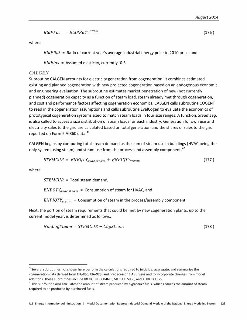
August 2014


𝐵𝑙𝑑𝑃𝐹𝑎𝑐 = 𝐵𝑙𝑑𝑃𝑅𝑎𝑡𝐵𝑙𝑑𝐸𝑙𝑎𝑠 (176 )

where

𝐵𝑙𝑑𝑃𝑅𝑎𝑡 = Ratio of current year’s average industrial energy price to 2010 price, and

𝐵𝑙𝑑𝐸𝑙𝑎𝑠 = Assumed elasticity, currently -0.5.

CALGEN Subroutine CALGEN accounts for electricity generation from cogeneration. It combines estimated existing and planned cogeneration with new projected cogeneration based on an endogenous economic and engineering evaluation. The subroutine estimates market penetration of new (not currently planned) cogeneration capacity as a function of steam load, steam already met through cogeneration, and cost and performance factors affecting cogeneration economics. CALGEN calls subroutine COGENT to read in the cogeneration assumptions and calls subroutine EvalCogen to evaluate the economics of prototypical cogeneration systems sized to match steam loads in four size ranges. A function, SteamSeg, is also called to access a size distribution of steam loads for each industry. Generation for own use and electricity sales to the grid are calculated based on total generation and the shares of sales to the grid reported on Form EIA-860 data.41

CALGEN begins by computing total steam demand as the sum of steam use in buildings (HVAC being the only system using steam) and steam use from the process and assembly component.42

𝑺𝑇𝐸𝑀𝐶𝑈𝑅 = 𝐸𝑁𝐵𝑄𝑇𝑌ℎ𝑣𝑎𝑐,𝑠𝑡𝑒𝑎𝑚 + 𝐸𝑁𝑃𝐼𝑄𝑇𝑌𝑠𝑡𝑒𝑎𝑚 (177 )

where

𝑆𝑇𝐸𝑀𝐶𝑈𝑅 = Total steam demand,

𝐸𝑁𝐵𝑄𝑇𝑌ℎ𝑣𝑎𝑐,𝑠𝑡𝑒𝑎𝑚 = Consumption of steam for HVAC, and

𝐸𝑁𝑃𝐼𝑄𝑇𝑌𝑠𝑡𝑒𝑎𝑚 = Consumption of steam in the process/assembly component.

Next, the portion of steam requirements that could be met by new cogeneration plants, up to the current model year, is determined as follows:

𝑁𝑜𝑛𝐶𝑜𝑔𝑆𝑡𝑒𝑎𝑚 = 𝑆𝑇𝐸𝑀𝐶𝑈𝑅 − 𝐶𝑜𝑔𝑆𝑡𝑒𝑎𝑚 (178 )

41Several subroutines not shown here perform the calculations required to initialize, aggregate, and summarize the cogeneration data derived from EIA-860, EIA-923, and predecessor EIA surveys and to incorporate changes from model additions. These subroutines include IRCOGEN, COGINIT, MECSLESS860, and ADDUPCOGS. 42This subroutine also calculates the amount of steam produced by byproduct fuels, which reduces the amount of steam required to be produced by purchased fuels.

August 2014


where

𝑁𝑜𝑛𝐶𝑜𝑔𝑆𝑡𝑒𝑎𝑚 = Non-cogenerated steam based on existing cogeneration capacity,

𝑆𝑇𝐸𝑀𝐶𝑈𝑅 = Total steam demand, and

𝐶𝑜𝑔𝑆𝑡𝑒𝑎𝑚 = Steam met by existing cogeneration units as of the last data year.

Non-cogeneration steam uses are disaggregated into eight size ranges, or segments, based on an exogenous data set providing the boiler size distribution for each industry. These data are accessed through the function 𝑆𝑡𝑒𝑎𝑚𝑆𝑒𝑔𝑙𝑜𝑎𝑑𝑠𝑒𝑔𝑚𝑒𝑛𝑡. It is assumed for this purpose that steam load segments are distributed in the same proportions as boiler capacity:

𝐴𝑔𝑔𝑆𝑡𝑒𝑎𝑚𝐿𝑜𝑎𝑑𝑙𝑜𝑎𝑑𝑠𝑒𝑔𝑚𝑒𝑛𝑡 = 𝑁𝑜𝑛𝐶𝑜𝑔𝑆𝑡𝑒𝑎𝑚 ∗ 𝑆𝑡𝑒𝑎𝑚𝑆𝑒𝑔𝑙𝑜𝑎𝑑𝑠𝑒𝑔𝑚𝑒𝑛𝑡 (179 )

where

𝐴𝑔𝑔𝑆𝑡𝑒𝑎𝑚𝐿𝑜𝑎𝑑𝑙𝑜𝑎𝑑𝑠𝑒𝑔𝑚𝑒𝑛𝑡 = Steam demand for a given load segment,

𝑁𝑜𝑛𝐶𝑜𝑔𝑆𝑡𝑒𝑎𝑚 = Non-cogenerated steam based on existing cogeneration capacity, and

𝑆𝑡𝑒𝑎𝑚𝑆𝑒𝑔𝑙𝑜𝑎𝑑𝑠𝑒𝑔𝑚𝑒𝑛𝑡 = The fraction of total steam in each of eight boiler firing ranges, in million Btu/hour, ranges are 1.5-3, 3-6.5, 6.5-10, 10-50, 50-100, 100-250, 250-500, and >500.

The average hourly steam load, 𝐴𝑣𝑔𝐻𝑜𝑢𝑟𝑙𝑦𝐿𝑜𝑎𝑑𝑙𝑜𝑎𝑑𝑠𝑒𝑔𝑚𝑒𝑛𝑡 in each segment is calculated from the aggregate steam load, 𝐴𝑔𝑔𝑆𝑡𝑒𝑎𝑚𝐿𝑜𝑎𝑑𝑙𝑜𝑎𝑑𝑠𝑒𝑔𝑚𝑒𝑛𝑡, based on 8,760 operating hours per year and converting from trillions to millions of Btu per hour:

𝐴𝑣𝑒𝐻𝑜𝑢𝑟𝑙𝑦𝐿𝑜𝑎𝑑𝑙𝑜𝑎𝑑𝑠𝑒𝑔𝑚𝑒𝑛𝑡 = 𝐴𝑔𝑔𝑆𝑡𝑒𝑎𝑚𝐿𝑜𝑎𝑑𝑙𝑜𝑎𝑑𝑠𝑒𝑔𝑚𝑒𝑛𝑡

0.008760 (180 )

The maximum technical potential for cogeneration is calculated assuming all non-cogeneration steam demand for each load segment is converted to cogeneration. This assumes that the technical potential is based on sizing systems, on average, to meet the average hourly steam load in each load segment. Using the power-steam ratio of the prototype cogeneration system selected for each load segment (from subroutine EvalCogen) this calculation is:

𝑇𝑒𝑐ℎ𝑃𝑜𝑡𝑙𝑜𝑎𝑑𝑠𝑒𝑔𝑚𝑒𝑛𝑡 = 𝐴𝑣𝑔𝐻𝑜𝑢𝑟𝑙𝑦𝐿𝑜𝑎𝑑𝑙𝑜𝑎𝑑𝑠𝑒𝑔𝑚𝑒𝑛𝑡 ∗ 𝑃𝑜𝑤𝑒𝑟𝑆𝑡𝑒𝑎𝑚𝑖𝑠𝑦𝑠 (181 )

where

𝑇𝑒𝑐ℎ𝑃𝑜𝑡𝑙𝑜𝑎𝑑𝑠𝑒𝑔𝑚𝑒𝑛𝑡 = Technical potential for cogeneration, in megawatts, for a load segment, irrespective of the economics,

𝐴𝑣𝑒𝐻𝑜𝑢𝑟𝑙𝑦𝐿𝑜𝑎𝑑𝑙𝑜𝑎𝑑𝑠𝑒𝑔𝑚𝑒𝑛𝑡 = Average hourly steam load in each load segment, and

𝑃𝑜𝑤𝑒𝑟𝑆𝑡𝑒𝑎𝑚𝑖𝑠𝑦𝑠 = Power-Steam ratio of the cogeneration system (equivalent to the ratio of electrical efficiency to thermal efficiency), 𝑖𝑠𝑦𝑠.

August 2014


The economic potential for cogeneration is estimated from the technical potential by applying the estimated fraction of that potential that will be realized over an extended time period, based on market acceptance criteria (as applied in subroutine EvalCogen):

𝐸𝑐𝑜𝑛𝑃𝑜𝑡𝑙𝑜𝑎𝑑𝑠𝑒𝑔𝑚𝑒𝑛𝑡 = 𝑇𝑒𝑐ℎ𝑃𝑜𝑡𝑙𝑜𝑎𝑑𝑠𝑒𝑔𝑚𝑒𝑛𝑡 ∗ 𝐸𝑐𝑜𝑛𝐹𝑟𝑎𝑐𝑙𝑜𝑎𝑑𝑠𝑒𝑔𝑚𝑒𝑛𝑡 (182 )

where

𝐸𝑐𝑜𝑛𝑃𝑜𝑡𝑙𝑜𝑎𝑑𝑠𝑒𝑔𝑚𝑒𝑛𝑡 = Economic potential for cogeneration in megawatts,

𝑇𝑒𝑐ℎ𝑃𝑜𝑡𝑙𝑜𝑎𝑑𝑠𝑒𝑔𝑚𝑒𝑛𝑡 = Technical potential for cogeneration, in megawatts, for a load segment if all cogeneration was adopted, irrespective of the economics, and

𝐸𝑐𝑜𝑛𝐹𝑟𝑎𝑐𝑙𝑜𝑎𝑑𝑠𝑒𝑔𝑚𝑒𝑛𝑡 = Economic fraction based on the payback period and the assumed payback acceptance curve.

Given the total economic potential for cogeneration, the amount of capacity that would be added in the current model year is given by:

𝐶𝑎𝑝𝐴𝑑𝑑𝑀𝑊𝑙𝑜𝑎𝑑𝑠𝑒𝑔𝑚𝑒𝑛𝑡 = 𝐸𝑐𝑜𝑛𝑃𝑜𝑡𝑙𝑜𝑎𝑑𝑠𝑒𝑔𝑚𝑒𝑛𝑡 ∗ 𝑃𝑒𝑛𝑒𝑡𝑟𝑎𝑡𝑖𝑜𝑛𝑅𝑎𝑡𝑒 (183 )

where

𝐶𝑎𝑝𝐴𝑑𝑑𝑀𝑊𝑙𝑜𝑎𝑑𝑠𝑒𝑔𝑚𝑒𝑛𝑡 = Cogeneration capacity added, in megawatts, for a load segment,

𝐸𝑐𝑜𝑛𝑃𝑜𝑡𝑙𝑜𝑎𝑑𝑠𝑒𝑔𝑚𝑒𝑛𝑡 = Economic potential for cogeneration in megawatts,

𝑃𝑒𝑛𝑒𝑡𝑟𝑎𝑡𝑖𝑜𝑛𝑅𝑎𝑡𝑒 = Constant annual rate of penetration, assumed to be 5% based on the economic potential being adopted over a 20-year time period; also includes “collaboration coefficients” provided by the American Council for an Energy-Efficient Economy (ACEEE)43 that show the relative likelihood of CHP adoption among U.S. regions. Based on the results of a study performed for EIA,44 which includes cogeneration system cost and performance characteristics, capacity additions are assumed to be natural-gas-fired except in certain industries that are known to use biomass for existing CHP, notably pulp and paper products. The corresponding generation and fuel use from these aggregated capacity additions are calculated from the assumed capacity factors and heat rates of the prototypical systems. The energy characteristics of the additions are used to increment the model’s cogeneration data arrays: capacity (COGCAP), generation (COGGEN), thermal output (COGTHR) and electricity-related-fuel use (COGELF). These arrays are all indexed by Census Division, year, industry, and fuel. Since the model runs at the Census Region level,

43 American Council for an Energy-Efficient Economy, “Challenges Facing Combined Heat and Power Today: A State-by-State Assessment,” September 2011, http://aceee.org/research-report/ie111, and U.S. Energy Information Administration, Office of Energy Analysis. 44 SENTECH Inc., Commercial and Industrial CHP Technology Cost and Performance Data for EIA, report prepared for the Office of Integrated Analysis and Forecasting, Energy Information Administration, Washington, DC, June 2010.

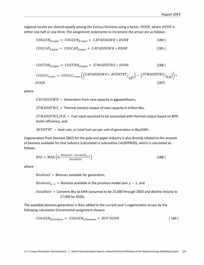
http://aceee.org/research-report/ie111

August 2014


regional results are shared equally among the Census Divisions using a factor, 𝐷𝑆𝐻𝑅, where 𝐷𝑆𝐻𝑅 is either one half or one third. The assignment statements to increment the arrays are as follows:

𝐶𝑂𝐺𝐺𝐸𝑁𝑑,𝑛𝑔𝑎𝑠 = 𝐶𝑂𝐺𝐺𝐸𝑁𝑑,𝑛𝑔𝑎𝑠 + 𝐶𝐴𝑃𝐴𝐷𝐷𝐺𝑊𝐻 ∗ 𝐷𝑆𝐻𝑅 (184 )

𝐶𝑂𝐺𝐶𝐴𝑃𝑑,𝑛𝑔𝑎𝑠 = 𝐶𝑂𝐺𝐶𝐴𝑃𝑑,𝑛𝑔𝑎𝑠 + 𝐶𝐴𝑃𝐴𝐷𝐷𝐺𝑊𝐻 ∗ 𝐷𝑆𝐻𝑅 (185 )

𝐶𝑂𝐺𝑇𝐻𝑅𝑑,𝑛𝑔𝑎𝑠 = 𝐶𝑂𝐺𝑇𝐻𝑅𝑑,𝑛𝑔𝑎𝑠 + 𝑆𝑇𝑀𝐴𝐷𝐷𝑇𝑅𝐼𝐿 ∗ 𝐷𝑆𝐻𝑅 (186 )

𝐶𝑂𝐺𝐸𝐿𝐹𝑑,𝑛𝑔𝑎𝑠 = 𝐶𝑂𝐺𝐸𝐿𝐹𝑑,𝑛𝑔𝑎𝑠 ��𝐶𝐴𝑃𝐴𝐷𝐷𝐺𝑊𝐻∗ 𝐴𝑉𝐸𝐻𝑇𝑅𝑇106� � − �𝑆𝑇𝑀𝐴𝐷𝐷𝑇𝑅𝐼𝐿 0.8� �� ∗

𝐷𝑆𝐻𝑅 (187)

where

𝐶𝐴𝑃𝐴𝐷𝐷𝐺𝑊𝐻 = Generation from new capacity in gigawatthours,

𝑆𝑇𝑀𝐴𝐷𝐷𝑇𝑅𝐼𝐿 = Thermal (steam) output of new capacity in trillion Btu,

𝑆𝑇𝑀𝐴𝐷𝐷𝑇𝑅𝐼𝐿/0.8 = Fuel input assumed to be associated with thermal output based on 80% boiler efficiency, and

𝐴𝑉𝐸𝐻𝑇𝑅𝑇 = Heat rate, or total fuel use per unit of generation in Btu/kWh.

Cogeneration from biomass (BIO) for the pulp and paper industry is also directly related to the amount of biomass available for that industry (calculated in subroutine CALBYPROD), which is calculated as follows:

𝐵𝐼𝑂 = 𝑀𝐴𝑋 �0, 𝐵𝑖𝑜𝐴𝑣𝑎𝑖𝑙− 𝐵𝑖𝑜𝐴𝑣𝑎𝑖𝑙𝑦−1𝐻𝑒𝑎𝑡𝑅𝑎𝑡𝑒

� (188 )

where

𝐵𝑖𝑜𝐴𝑣𝑎𝑖𝑙 = Biomass available for generation,

𝐵𝑖𝑜𝐴𝑣𝑎𝑖𝑙𝑦−1 = Biomass available in the previous model year 𝑦 − 1, and

𝐻𝑒𝑎𝑡𝑅𝑎𝑡𝑒 = Converts Btu to kWh (assumed to be 25,000 through 2003 and decline linearly to 17,000 by 2020).

The available biomass generation is then added to the current year’s cogeneration arrays by the following calculation (incremental assignment shown):

𝐶𝑂𝐺𝐺𝐸𝑁𝑑,𝑏𝑖𝑜𝑚𝑎𝑠𝑠 = 𝐶𝑂𝐺𝐺𝐸𝑁𝑑,𝑏𝑖𝑜𝑚𝑎𝑠𝑠 + 𝐵𝐼𝑂∗𝐷𝑆𝐻𝑅 ( 189 )

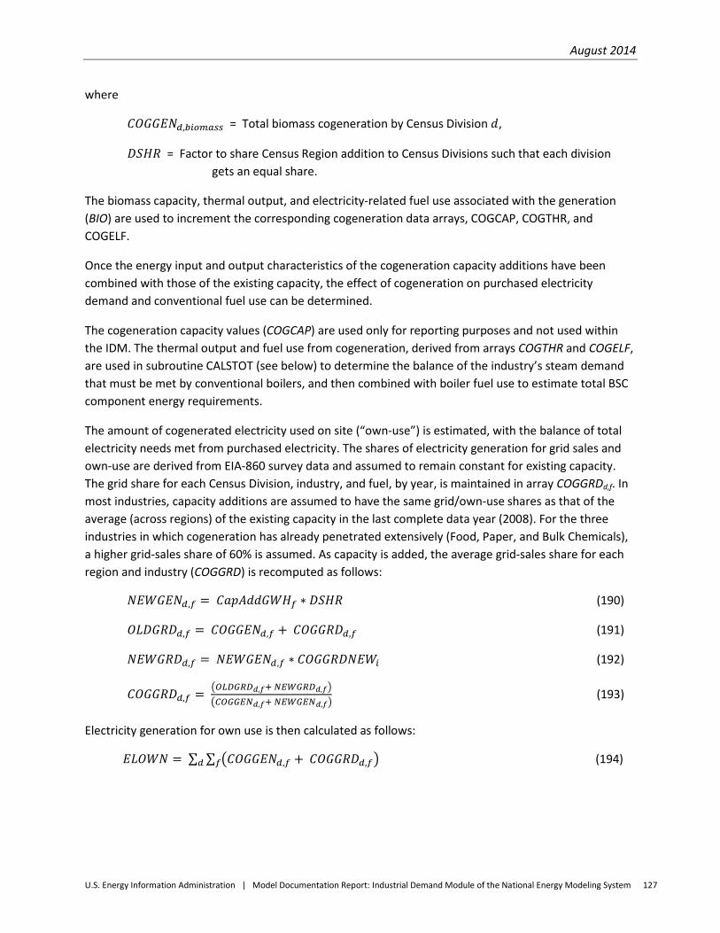
August 2014


where

𝐶𝑂𝐺𝐺𝐸𝑁𝑑,𝑏𝑖𝑜𝑚𝑎𝑠𝑠 = Total biomass cogeneration by Census Division 𝑑,

𝐷𝑆𝐻𝑅 = Factor to share Census Region addition to Census Divisions such that each division gets an equal share.

The biomass capacity, thermal output, and electricity-related fuel use associated with the generation (BIO) are used to increment the corresponding cogeneration data arrays, COGCAP, COGTHR, and COGELF.

Once the energy input and output characteristics of the cogeneration capacity additions have been combined with those of the existing capacity, the effect of cogeneration on purchased electricity demand and conventional fuel use can be determined.

The cogeneration capacity values (COGCAP) are used only for reporting purposes and not used within the IDM. The thermal output and fuel use from cogeneration, derived from arrays COGTHR and COGELF, are used in subroutine CALSTOT (see below) to determine the balance of the industry’s steam demand that must be met by conventional boilers, and then combined with boiler fuel use to estimate total BSC component energy requirements.

The amount of cogenerated electricity used on site (“own-use”) is estimated, with the balance of total electricity needs met from purchased electricity. The shares of electricity generation for grid sales and own-use are derived from EIA-860 survey data and assumed to remain constant for existing capacity. The grid share for each Census Division, industry, and fuel, by year, is maintained in array COGGRDd,f. In most industries, capacity additions are assumed to have the same grid/own-use shares as that of the average (across regions) of the existing capacity in the last complete data year (2008). For the three industries in which cogeneration has already penetrated extensively (Food, Paper, and Bulk Chemicals), a higher grid-sales share of 60% is assumed. As capacity is added, the average grid-sales share for each region and industry (COGGRD) is recomputed as follows:

𝑁𝐸𝑊𝐺𝐸𝑁𝑑,𝑓 = 𝐶𝑎𝑝𝐴𝑑𝑑𝐺𝑊𝐻𝑓 ∗ 𝐷𝑆𝐻𝑅 (190)

𝑂𝐿𝐷𝐺𝑅𝐷𝑑,𝑓 = 𝐶𝑂𝐺𝐺𝐸𝑁𝑑,𝑓 + 𝐶𝑂𝐺𝐺𝑅𝐷𝑑,𝑓 (191)

𝑁𝐸𝑊𝐺𝑅𝐷𝑑,𝑓 = 𝑁𝐸𝑊𝐺𝐸𝑁𝑑,𝑓 ∗ 𝐶𝑂𝐺𝐺𝑅𝐷𝑁𝐸𝑊𝑖 (192)

𝐶𝑂𝐺𝐺𝑅𝐷𝑑,𝑓 = �𝑂𝐿𝐷𝐺𝑅𝐷𝑑,𝑓+ 𝑁𝐸𝑊𝐺𝑅𝐷𝑑,𝑓��𝐶𝑂𝐺𝐺𝐸𝑁𝑑,𝑓+ 𝑁𝐸𝑊𝐺𝐸𝑁𝑑,𝑓�

(193)

Electricity generation for own use is then calculated as follows:

𝐸𝐿𝑂𝑊𝑁 = ∑ ∑ �𝐶𝑂𝐺𝐺𝐸𝑁𝑑,𝑓 + 𝐶𝑂𝐺𝐺𝑅𝐷𝑑,𝑓�𝑓𝑑 (194)

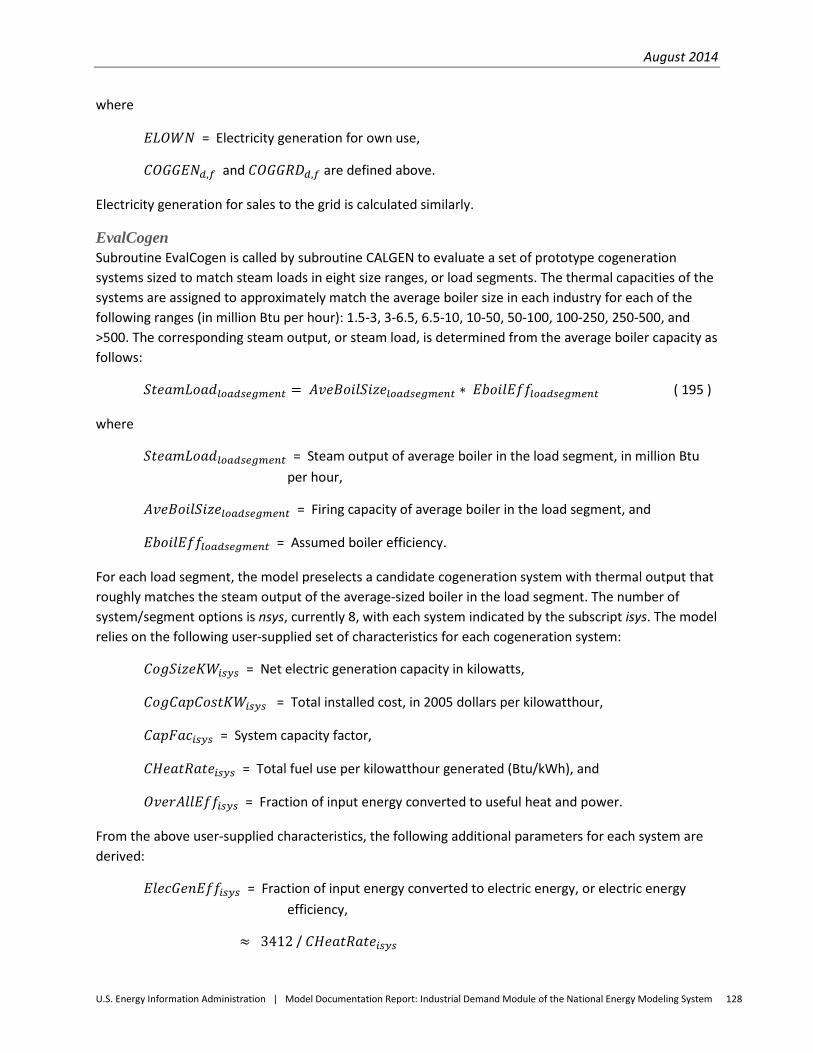
August 2014


where

𝐸𝐿𝑂𝑊𝑁 = Electricity generation for own use,

𝐶𝑂𝐺𝐺𝐸𝑁𝑑,𝑓 and 𝐶𝑂𝐺𝐺𝑅𝐷𝑑,𝑓 are defined above.

Electricity generation for sales to the grid is calculated similarly.

EvalCogen Subroutine EvalCogen is called by subroutine CALGEN to evaluate a set of prototype cogeneration systems sized to match steam loads in eight size ranges, or load segments. The thermal capacities of the systems are assigned to approximately match the average boiler size in each industry for each of the following ranges (in million Btu per hour): 1.5-3, 3-6.5, 6.5-10, 10-50, 50-100, 100-250, 250-500, and >500. The corresponding steam output, or steam load, is determined from the average boiler capacity as follows:

𝑆𝑡𝑒𝑎𝑚𝐿𝑜𝑎𝑑𝑙𝑜𝑎𝑑𝑠𝑒𝑔𝑚𝑒𝑛𝑡 = 𝐴𝑣𝑒𝐵𝑜𝑖𝑙𝑆𝑖𝑧𝑒𝑙𝑜𝑎𝑑𝑠𝑒𝑔𝑚𝑒𝑛𝑡 ∗ 𝐸𝑏𝑜𝑖𝑙𝐸𝑓𝑓𝑙𝑜𝑎𝑑𝑠𝑒𝑔𝑚𝑒𝑛𝑡 ( 195 )

where

𝑆𝑡𝑒𝑎𝑚𝐿𝑜𝑎𝑑𝑙𝑜𝑎𝑑𝑠𝑒𝑔𝑚𝑒𝑛𝑡 = Steam output of average boiler in the load segment, in million Btu per hour,

𝐴𝑣𝑒𝐵𝑜𝑖𝑙𝑆𝑖𝑧𝑒𝑙𝑜𝑎𝑑𝑠𝑒𝑔𝑚𝑒𝑛𝑡 = Firing capacity of average boiler in the load segment, and

𝐸𝑏𝑜𝑖𝑙𝐸𝑓𝑓𝑙𝑜𝑎𝑑𝑠𝑒𝑔𝑚𝑒𝑛𝑡 = Assumed boiler efficiency.

For each load segment, the model preselects a candidate cogeneration system with thermal output that roughly matches the steam output of the average-sized boiler in the load segment. The number of system/segment options is nsys, currently 8, with each system indicated by the subscript isys. The model relies on the following user-supplied set of characteristics for each cogeneration system:

𝐶𝑜𝑔𝑆𝑖𝑧𝑒𝐾𝑊𝑖𝑠𝑦𝑠 = Net electric generation capacity in kilowatts,

𝐶𝑜𝑔𝐶𝑎𝑝𝐶𝑜𝑠𝑡𝐾𝑊𝑖𝑠𝑦𝑠 = Total installed cost, in 2005 dollars per kilowatthour,

𝐶𝑎𝑝𝐹𝑎𝑐𝑖𝑠𝑦𝑠 = System capacity factor,

𝐶𝐻𝑒𝑎𝑡𝑅𝑎𝑡𝑒𝑖𝑠𝑦𝑠 = Total fuel use per kilowatthour generated (Btu/kWh), and

𝑂𝑣𝑒𝑟𝐴𝑙𝑙𝐸𝑓𝑓𝑖𝑠𝑦𝑠 = Fraction of input energy converted to useful heat and power.

From the above user-supplied characteristics, the following additional parameters for each system are derived:

𝐸𝑙𝑒𝑐𝐺𝑒𝑛𝐸𝑓𝑓𝑖𝑠𝑦𝑠 = Fraction of input energy converted to electric energy, or electric energy efficiency,

≈ 3412 / 𝐶𝐻𝑒𝑎𝑡𝑅𝑎𝑡𝑒𝑖𝑠𝑦𝑠

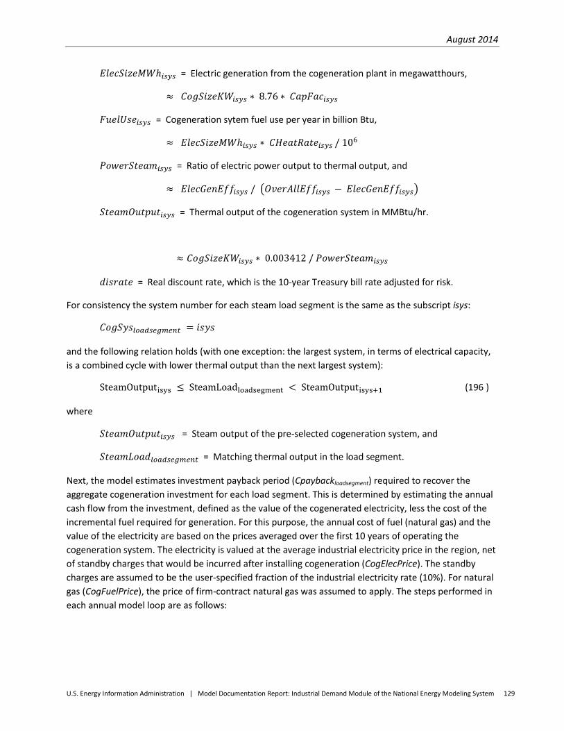
August 2014


𝐸𝑙𝑒𝑐𝑆𝑖𝑧𝑒𝑀𝑊ℎ𝑖𝑠𝑦𝑠 = Electric generation from the cogeneration plant in megawatthours,

≈ 𝐶𝑜𝑔𝑆𝑖𝑧𝑒𝐾𝑊𝑖𝑠𝑦𝑠 ∗ 8.76 ∗ 𝐶𝑎𝑝𝐹𝑎𝑐𝑖𝑠𝑦𝑠

𝐹𝑢𝑒𝑙𝑈𝑠𝑒𝑖𝑠𝑦𝑠 = Cogeneration sytem fuel use per year in billion Btu,

≈ 𝐸𝑙𝑒𝑐𝑆𝑖𝑧𝑒𝑀𝑊ℎ𝑖𝑠𝑦𝑠 ∗ 𝐶𝐻𝑒𝑎𝑡𝑅𝑎𝑡𝑒𝑖𝑠𝑦𝑠 / 106

𝑃𝑜𝑤𝑒𝑟𝑆𝑡𝑒𝑎𝑚𝑖𝑠𝑦𝑠 = Ratio of electric power output to thermal output, and

≈ 𝐸𝑙𝑒𝑐𝐺𝑒𝑛𝐸𝑓𝑓𝑖𝑠𝑦𝑠 / �𝑂𝑣𝑒𝑟𝐴𝑙𝑙𝐸𝑓𝑓𝑖𝑠𝑦𝑠 − 𝐸𝑙𝑒𝑐𝐺𝑒𝑛𝐸𝑓𝑓𝑖𝑠𝑦𝑠�

𝑆𝑡𝑒𝑎𝑚𝑂𝑢𝑡𝑝𝑢𝑡𝑖𝑠𝑦𝑠 = Thermal output of the cogeneration system in MMBtu/hr.

≈ 𝐶𝑜𝑔𝑆𝑖𝑧𝑒𝐾𝑊𝑖𝑠𝑦𝑠 ∗ 0.003412 / 𝑃𝑜𝑤𝑒𝑟𝑆𝑡𝑒𝑎𝑚𝑖𝑠𝑦𝑠

𝑑𝑖𝑠𝑟𝑎𝑡𝑒 = Real discount rate, which is the 10-year Treasury bill rate adjusted for risk.

For consistency the system number for each steam load segment is the same as the subscript isys:

𝐶𝑜𝑔𝑆𝑦𝑠𝑙𝑜𝑎𝑑𝑠𝑒𝑔𝑚𝑒𝑛𝑡 = 𝑖𝑠𝑦𝑠

and the following relation holds (with one exception: the largest system, in terms of electrical capacity, is a combined cycle with lower thermal output than the next largest system):

SteamOutputisys ≤ SteamLoadloadsegment < SteamOutputisys+1 (196 )

where

𝑆𝑡𝑒𝑎𝑚𝑂𝑢𝑡𝑝𝑢𝑡𝑖𝑠𝑦𝑠 = Steam output of the pre-selected cogeneration system, and

𝑆𝑡𝑒𝑎𝑚𝐿𝑜𝑎𝑑𝑙𝑜𝑎𝑑𝑠𝑒𝑔𝑚𝑒𝑛𝑡 = Matching thermal output in the load segment.

Next, the model estimates investment payback period (Cpaybackloadsegment) required to recover the aggregate cogeneration investment for each load segment. This is determined by estimating the annual cash flow from the investment, defined as the value of the cogenerated electricity, less the cost of the incremental fuel required for generation. For this purpose, the annual cost of fuel (natural gas) and the value of the electricity are based on the prices averaged over the first 10 years of operating the cogeneration system. The electricity is valued at the average industrial electricity price in the region, net of standby charges that would be incurred after installing cogeneration (CogElecPrice). The standby charges are assumed to be the user-specified fraction of the industrial electricity rate (10%). For natural gas (CogFuelPrice), the price of firm-contract natural gas was assumed to apply. The steps performed in each annual model loop are as follows:

August 2014


Determine annual fuel cost of the aggregated cogeneration systems in each load segment:

𝐹𝑢𝑒𝑙𝐶𝑜𝑠𝑡𝑙𝑜𝑎𝑑𝑠𝑒𝑔𝑚𝑒𝑛𝑡 = 𝐹𝑢𝑒𝑙𝑈𝑠𝑒𝑖𝑠𝑦𝑠 ∗ 𝐶𝑜𝑔𝐹𝑢𝑒𝑙𝑃𝑟𝑖𝑐𝑒 (197)

Determine the annual fuel use and cost of operating the existing system (conventional boiler):

𝐸𝑥𝑖𝑠𝑡𝐹𝑢𝑒𝑙𝑈𝑠𝑒𝑙𝑜𝑎𝑑𝑠𝑒𝑔𝑚𝑒𝑛𝑡 = 𝑆𝑡𝑒𝑎𝑚𝑂𝑢𝑡𝑝𝑢𝑡𝑖𝑠𝑦𝑠∗8.76∗𝐶𝑎𝑝𝐹𝑎𝑐𝑖𝑠𝑦𝑠𝐸𝑏𝑜𝑖𝑙𝐸𝑓𝑓𝑙𝑜𝑎𝑑𝑠𝑒𝑔𝑚𝑒𝑛𝑡

(198)

𝐸𝑥𝑖𝑠𝑡𝐹𝑢𝑒𝑙𝐶𝑜𝑠𝑡𝑙𝑜𝑎𝑑𝑠𝑒𝑔𝑚𝑒𝑛𝑡 = 𝐸𝑥𝑖𝑠𝑡𝐹𝑢𝑒𝑙𝑈𝑠𝑒𝑙𝑜𝑎𝑑𝑠𝑒𝑔𝑚𝑒𝑛𝑡 ∗ 𝐶𝑜𝑔𝐹𝑢𝑒𝑙𝑃𝑟𝑖𝑐𝑒 (199)

Determine incremental fuel cost and the value of cogenerated electricity:

𝐼𝑛𝑐𝑟𝐹𝑢𝑒𝑙𝐶𝑜𝑠𝑡𝑙𝑜𝑎𝑑𝑠𝑒𝑔𝑚𝑒𝑛𝑡 = 𝐹𝑢𝑒𝑙𝐶𝑜𝑠𝑡𝑙𝑜𝑎𝑑𝑠𝑒𝑔𝑚𝑒𝑛𝑡 − 𝐸𝑥𝑖𝑠𝑡𝐹𝑢𝑒𝑙𝐶𝑜𝑠𝑡𝑙𝑜𝑎𝑑𝑠𝑒𝑔𝑚𝑒𝑛𝑡 (200)

𝐸𝑙𝑒𝑐𝑉𝑎𝑙𝑢𝑒𝑙𝑜𝑎𝑑𝑠𝑒𝑔𝑚𝑒𝑛𝑡 = 𝐸𝑙𝑒𝑐𝑆𝑖𝑧𝑒𝑀𝑊ℎ𝑖𝑠𝑦𝑠 ∗ 𝐶𝑜𝑔𝐸𝑙𝑒𝑐𝑃𝑟𝑖𝑐𝑒 ∗ 0.003412 (201)

Determine the cash flow, or operating profit, of the investment:

𝑂𝑝𝑒𝑟𝑃𝑟𝑜𝑓𝑖𝑡𝑙𝑜𝑎𝑑𝑠𝑒𝑔𝑚𝑒𝑛𝑡 = 𝐸𝑙𝑒𝑐𝑉𝑎𝑙𝑢𝑒𝑙𝑜𝑎𝑑𝑠𝑒𝑔𝑚𝑒𝑛𝑡 − 𝐼𝑛𝑐𝑟𝐹𝑢𝑒𝑙𝐶𝑜𝑠𝑡𝑙𝑜𝑎𝑑𝑠𝑒𝑔𝑚𝑒𝑛𝑡 (202)

Determine the investment capital cost and the investment payback period:

𝐼𝑛𝑣𝑒𝑠𝑡𝑚𝑒𝑛𝑡𝑙𝑜𝑎𝑑𝑠𝑒𝑔𝑚𝑒𝑛𝑡 = 𝐶𝑜𝑔𝑆𝑖𝑧𝑒𝐾𝑊𝑙𝑖𝑠𝑦𝑠 ∗ 𝐶𝑜𝑔𝐶𝑎𝑝𝐶𝑜𝑠𝑡𝐾𝑊𝑖𝑠𝑦𝑠 (203)

𝐶𝑃𝑎𝑦𝐵𝑎𝑐𝑘𝑙𝑜𝑎𝑑𝑠𝑒𝑔𝑚𝑒𝑛𝑡 = 𝐼𝑛𝑣𝑒𝑠𝑡𝑚𝑒𝑛𝑡𝑙𝑜𝑎𝑑𝑠𝑒𝑔𝑚𝑒𝑛𝑡

𝑂𝑝𝑒𝑟𝑃𝑟𝑜𝑓𝑖𝑡𝑙𝑜𝑎𝑑𝑠𝑒𝑔𝑚𝑒𝑛𝑡 /(1+𝑑𝑖𝑠𝑟𝑎𝑡𝑒)𝑦𝑒𝑎𝑟 (204)

Given the payback for the aggregated system evaluated for each load segment, the model estimates the fraction of total technical potential considered economical. This calculation uses an assumed distribution of required investment payback periods, referred to as the payback acceptance curve. A table of assumptions is used containing acceptance rates for each integer payback period from 0 to 12 years. To obtain an acceptance fraction, or economic fraction, from a non-integer value for payback, a linear interpolation is done. The economic fraction is determined from a table lookup and interpolation function called Acceptance.

Given the table of acceptance fractions, the number of rows in the table (13), and the payback period for the load segment, the calculation is:

𝐸𝑐𝑜𝑛𝐹𝑟𝑎𝑐𝑙𝑜𝑎𝑑𝑠𝑒𝑔𝑚𝑒𝑛𝑡 = 𝐴𝑐𝑐𝑒𝑝𝑡𝑎𝑛𝑐𝑒 �𝐴𝑐𝑐𝑒𝑝𝑡𝐹𝑟𝑎𝑐, 13,𝐶𝑃𝑎𝑦𝐵𝑎𝑐𝑘𝑙𝑜𝑎𝑑𝑠𝑒𝑔𝑚𝑒𝑛𝑡� (205)

where

𝐸𝑐𝑜𝑛𝐹𝑟𝑎𝑐𝑙𝑜𝑎𝑑𝑠𝑒𝑔𝑚𝑒𝑛𝑡 = Fraction of cogeneration investments adopted based on payback period of acceptance assumptions,

𝐴𝑐𝑐𝑒𝑝𝑡𝐹𝑟𝑎𝑐 = Array of payback acceptance rates corresponding to integer payback periods ranging from 0 to 12 (13 rates altogether), and

𝐶𝑃𝑎𝑦𝐵𝑎𝑐𝑘𝑙𝑜𝑎𝑑𝑠𝑒𝑔𝑚𝑒𝑛𝑡 = Cogeneration investment payback period.

August 2014


CALSTOT CALSTOT calculates total fuel consumption in the BSC component based on total steam demand within an industry (STEMCUR). Steam demand and fuel consumption (in BTU) are allocated between cogeneration and conventional boilers. Fuel use and steam demand from cogeneration, calculated in subroutine CALGEN, are treated as inputs to this subroutine.

Steam from cogeneration (COGSTEAM) is obtained by summing the cogeneration thermal output (in array COGTHR) across fuels and Census Divisions. Steam demand to be met by conventional boilers (NonCOGSTEAM) is equal to total steam demand (STEMCUR) minus cogeneration steam (COGSTEAM) production.

The estimated consumption of fuel for cogeneration is stored in two variables: fuel used to generate electricity (COGELF) and fuel associated with the thermal output (COGTHR). The fuel associated with the thermal output assumes a hypothetical 80% efficiency, so it is computed as COGTHR divided by 0.8. Thus, total cogeneration system fuel use, FuelSysf, is given by:

𝐹𝑢𝑒𝑙𝑆𝑦𝑠𝑓 = ∑ 𝐶𝑂𝐺𝐸𝐿𝐹𝑑,𝑓𝑑 + �𝐶𝑂𝐺𝑂𝑇𝐻𝑅𝑑,𝑓/0.8� (206)

Conventional boiler fuel use is split between biomass-derived fuels and fossil fuels. The total available biomass is calculated as byproduct fuels (BYPBSCRbiofuel). Some of it is used in cogeneration; the remainder of the available biomass (AvailBiomass) is assumed to be used as boiler fuel. The amount of steam from this biomass (BIOSTEAM) is estimated based on assumed biomass boiler efficiency (0.69).

The steam demand that must be met through fossil-fired boilers is the total non-cogenerated steam (NonCogSteam) less the bio fueled steam (BIOSTEAM or NonCogFosSteam). A trial estimate for total fossil fuel for boilers is derived from NonCogFosSteam assuming average boiler efficiency across fuels.

Allocating this total to specific fuels in a manner consistent with MECS data is difficult. The MECS data indicate only the total amounts of indirect fuels associated with boilers and cogeneration, so fuel-specific boiler use cannot be computed from MECS alone. Because fuel use and thermal output data is taken from EIA Form 860, deriving an estimated conventional boiler fuel requirement consistent with MECS requires a calibration step. The model calibrates the fuel volumes to ensure that the sum of the cogeneration fuel and conventional boiler fuel (from Form 860) equals the MECS indirect fuel estimate in the base year.

The derivation of the boiler fuel calibration factor is based on the results of subroutine MecsLess860, which, as its name implies, calculates the difference between total MECS indirect fuels (BSCbsyr) and the cogeneration (or CHP) fuel use from Form 860 (CHPbsyr), and stores it in array BOILBSYR. A separate calibration is performed for biomass- and fossil-fueled boilers. The calibration factor for fossil fuels is computed as follows in model year 2010:

𝐸𝑠𝑡𝑖𝑚𝑎𝑡𝑒𝑑 = 𝑁𝑜𝑛𝐶𝑜𝑔𝐹𝑜𝑠𝑆𝑡𝑒𝑎𝑚/ 0.8

𝐼𝑚𝑝𝑙𝑖𝑒𝑑 = �𝐵𝑂𝐼𝐿𝐵𝑆𝑌𝑅𝑓𝑓

August 2014


𝐶𝐴𝐿𝐼𝐵2002_𝐹𝑂𝑆 = 𝐼𝑚𝑝𝑙𝑖𝑒𝑑/ 𝐸𝑠𝑡𝑖𝑚𝑎𝑡𝑒𝑑

where

𝐸𝑠𝑡𝑖𝑚𝑎𝑡𝑒𝑑 = Preliminary estimate of fossil fuel use from conventional boilers,

𝐼𝑚𝑝𝑙𝑖𝑒𝑑 = Conventional boiler fuel use,

𝐵𝑂𝐼𝐿𝐵𝑆𝑌𝑅𝑓 = Ratio of MECS and Form 860860 for each boiler fuel 𝑓, and

𝐶𝐴𝐿𝐼𝐵𝐵𝑆𝑌𝑅_𝐹𝑂𝑆 = Calibration factor for conventional boiler fuel use.

In the projection, the calibration factors for the base year adjust the preliminary estimates to yield the estimated non-cogeneration fossil fuel:

𝑁𝑜𝑛𝐶𝑜𝑔𝐹𝑜𝑠𝐹𝑢𝑒𝑙 = 𝑁𝑜𝑛𝐶𝑜𝑔𝐹𝑜𝑠𝑆𝑡𝑒𝑎𝑚 ∗ 𝐵𝑆𝑆𝐻𝑅𝑓 ( 207 )

where

𝑁𝑜𝑛𝐶𝑜𝑔𝐹𝑜𝑠𝐹𝑢𝑒𝑙 = Non-cogeneration (conventional) fossil fuel use in boilers, calibrated to match MECS when combined with 860 cogeneration data; and

𝐵𝑆𝑆𝐻𝑅𝑓 = Boiler fuel shares estimated in subroutine CALBSC.

𝑁𝑜𝑛𝐶𝑜𝑔𝐹𝑜𝑠𝑆𝑡𝑒𝑎𝑚 is defined above.

Conventional boiler fuel use (FuelFosSteamf) is allocated to fuels based on fuel shares adjusted for price changes since 2010 and fuel-specific efficiencies:

𝐹𝑢𝑒𝑙𝐹𝑜𝑠𝑆𝑡𝑒𝑎𝑚𝑓 = �𝑁𝑜𝑛𝐶𝑜𝑔𝐹𝑜𝑠𝐹𝑢𝑒𝑙 ÷ 𝑏𝑒𝑓𝑓𝑓� ∗ 𝐶𝐴𝐿𝐼𝐵𝐵𝑆𝑌𝑅_𝐹𝑂𝑆 ( 208 )

where

𝑏𝑒𝑓𝑓𝑓 = Boiler efficiency by fuel given in Table 10.

𝐶𝐴𝐿𝐼𝐵𝐵𝑆𝑌𝑅_𝐹𝑂𝑆 is defined above.

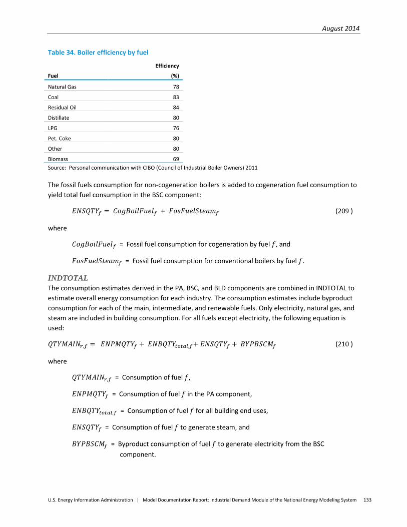
August 2014


Table 34. Boiler efficiency by fuel

Fuel

Efficiency

(%)

Natural Gas 78

Coal 83

Residual Oil 84

Distillate 80

LPG 76

Pet. Coke 80

Other 80

Biomass 69 Source: Personal communication with CIBO (Council of Industrial Boiler Owners) 2011

The fossil fuels consumption for non-cogeneration boilers is added to cogeneration fuel consumption to yield total fuel consumption in the BSC component:

𝐸𝑁𝑆𝑄𝑇𝑌𝑓 = 𝐶𝑜𝑔𝐵𝑜𝑖𝑙𝐹𝑢𝑒𝑙𝑓 + 𝐹𝑜𝑠𝐹𝑢𝑒𝑙𝑆𝑡𝑒𝑎𝑚𝑓 (209 )

where

𝐶𝑜𝑔𝐵𝑜𝑖𝑙𝐹𝑢𝑒𝑙𝑓 = Fossil fuel consumption for cogeneration by fuel 𝑓, and

𝐹𝑜𝑠𝐹𝑢𝑒𝑙𝑆𝑡𝑒𝑎𝑚𝑓 = Fossil fuel consumption for conventional boilers by fuel 𝑓.

INDTOTAL The consumption estimates derived in the PA, BSC, and BLD components are combined in INDTOTAL to estimate overall energy consumption for each industry. The consumption estimates include byproduct consumption for each of the main, intermediate, and renewable fuels. Only electricity, natural gas, and steam are included in building consumption. For all fuels except electricity, the following equation is used:

𝑄𝑇𝑌𝑀𝐴𝐼𝑁𝑟,𝑓 = 𝐸𝑁𝑃𝑀𝑄𝑇𝑌𝑓 + 𝐸𝑁𝐵𝑄𝑇𝑌𝑡𝑜𝑡𝑎𝑙,𝑓+ 𝐸𝑁𝑆𝑄𝑇𝑌𝑓 + 𝐵𝑌𝑃𝐵𝑆𝐶𝑀𝑓 (210 )

where

𝑄𝑇𝑌𝑀𝐴𝐼𝑁𝑟,𝑓 = Consumption of fuel 𝑓,

𝐸𝑁𝑃𝑀𝑄𝑇𝑌𝑓 = Consumption of fuel 𝑓 in the PA component,

𝐸𝑁𝐵𝑄𝑇𝑌𝑡𝑜𝑡𝑎𝑙,𝑓 = Consumption of fuel 𝑓 for all building end uses,

𝐸𝑁𝑆𝑄𝑇𝑌𝑓 = Consumption of fuel 𝑓 to generate steam, and

𝐵𝑌𝑃𝐵𝑆𝐶𝑀𝑓 = Byproduct consumption of fuel 𝑓 to generate electricity from the BSC component.

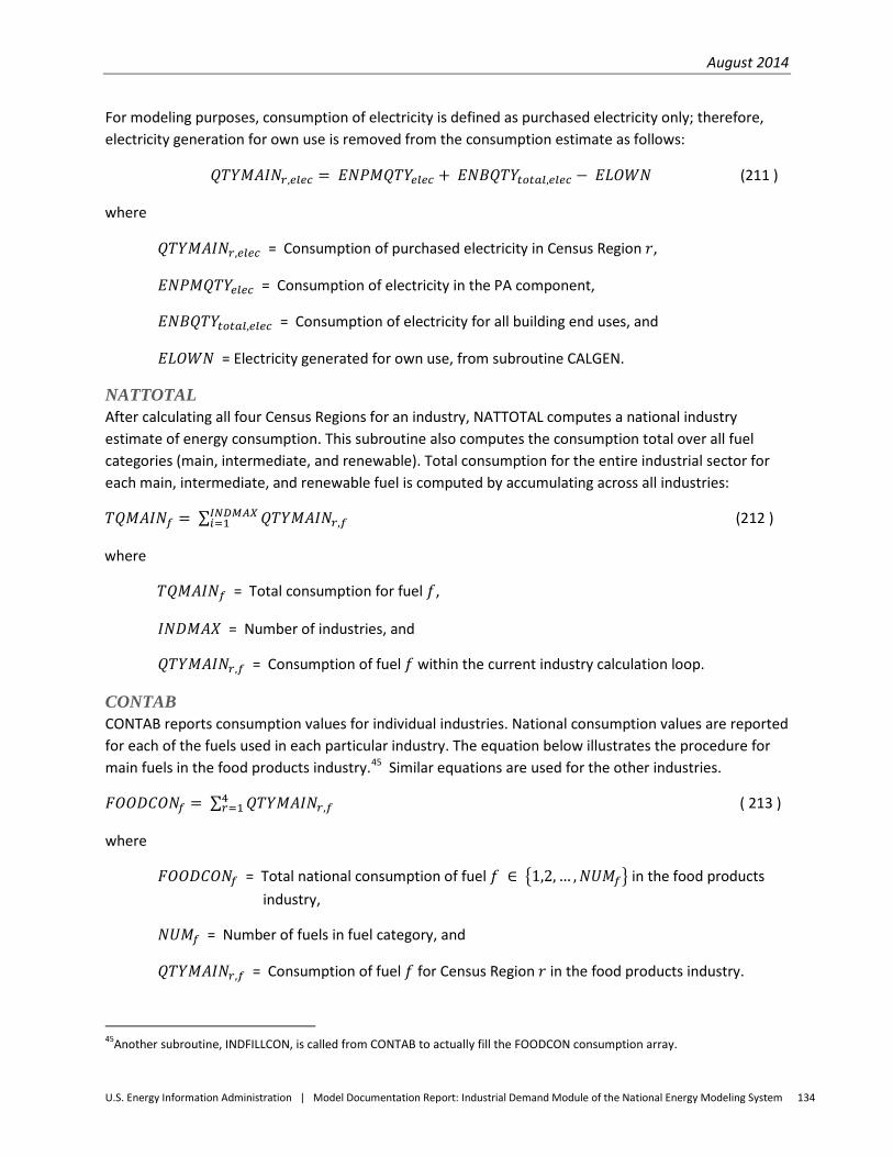
August 2014


For modeling purposes, consumption of electricity is defined as purchased electricity only; therefore, electricity generation for own use is removed from the consumption estimate as follows:

𝑄𝑇𝑌𝑀𝐴𝐼𝑁𝑟,𝑒𝑙𝑒𝑐 = 𝐸𝑁𝑃𝑀𝑄𝑇𝑌𝑒𝑙𝑒𝑐 + 𝐸𝑁𝐵𝑄𝑇𝑌𝑡𝑜𝑡𝑎𝑙,𝑒𝑙𝑒𝑐 − 𝐸𝐿𝑂𝑊𝑁 (211 )

where

𝑄𝑇𝑌𝑀𝐴𝐼𝑁𝑟,𝑒𝑙𝑒𝑐 = Consumption of purchased electricity in Census Region 𝑟,

𝐸𝑁𝑃𝑀𝑄𝑇𝑌𝑒𝑙𝑒𝑐 = Consumption of electricity in the PA component,

𝐸𝑁𝐵𝑄𝑇𝑌𝑡𝑜𝑡𝑎𝑙,𝑒𝑙𝑒𝑐 = Consumption of electricity for all building end uses, and

𝐸𝐿𝑂𝑊𝑁 = Electricity generated for own use, from subroutine CALGEN.

NATTOTAL After calculating all four Census Regions for an industry, NATTOTAL computes a national industry estimate of energy consumption. This subroutine also computes the consumption total over all fuel categories (main, intermediate, and renewable). Total consumption for the entire industrial sector for each main, intermediate, and renewable fuel is computed by accumulating across all industries:

𝑇𝑄𝑀𝐴𝐼𝑁𝑓 = ∑ 𝑄𝑇𝑌𝑀𝐴𝐼𝑁𝑟,𝑓𝐼𝑁𝐷𝑀𝐴𝑋𝑖=1 (212 )

where

𝑇𝑄𝑀𝐴𝐼𝑁𝑓 = Total consumption for fuel 𝑓,

𝐼𝑁𝐷𝑀𝐴𝑋 = Number of industries, and

𝑄𝑇𝑌𝑀𝐴𝐼𝑁𝑟,𝑓 = Consumption of fuel 𝑓 within the current industry calculation loop.

CONTAB CONTAB reports consumption values for individual industries. National consumption values are reported for each of the fuels used in each particular industry. The equation below illustrates the procedure for main fuels in the food products industry.45 Similar equations are used for the other industries.

𝐹𝑂𝑂𝐷𝐶𝑂𝑁𝑓 = ∑ 𝑄𝑇𝑌𝑀𝐴𝐼𝑁𝑟,𝑓4𝑟=1 ( 213 )

where

𝐹𝑂𝑂𝐷𝐶𝑂𝑁𝑓 = Total national consumption of fuel 𝑓 ∈ �1,2, … ,𝑁𝑈𝑀𝑓� in the food products industry,

𝑁𝑈𝑀𝑓 = Number of fuels in fuel category, and

𝑄𝑇𝑌𝑀𝐴𝐼𝑁𝑟,𝑓 = Consumption of fuel 𝑓 for Census Region 𝑟 in the food products industry.

45Another subroutine, INDFILLCON, is called from CONTAB to actually fill the FOODCON consumption array.

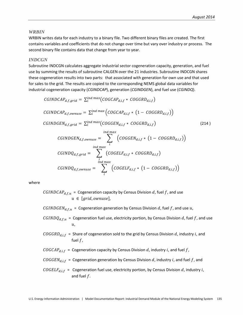
August 2014


WRBIN WRBIN writes data for each industry to a binary file. Two different binary files are created. The first contains variables and coefficients that do not change over time but vary over industry or process. The second binary file contains data that change from year to year.

INDCGN Subroutine INDCGN calculates aggregate industrial sector cogeneration capacity, generation, and fuel use by summing the results of subroutine CALGEN over the 21 industries. Subroutine INDCGN shares these cogeneration results into two parts: that associated with generation for own use and that used for sales to the grid. The results are copied to the corresponding NEMS global data variables for industrial cogeneration capacity (CGINDCAP), generation (CGINDGEN), and fuel use (CGINDQ).

𝐶𝐺𝐼𝑁𝐷𝐶𝐴𝑃𝑑,𝑓,𝑔𝑟𝑖𝑑 = ∑ �𝐶𝑂𝐺𝐶𝐴𝑃𝑑,𝑖,𝑓 ∗ 𝐶𝑂𝐺𝐺𝑅𝐷𝑑,𝑖,𝑓�𝑖𝑛𝑑 𝑚𝑎𝑥𝑖

𝐶𝐺𝐼𝑁𝐷𝐶𝐴𝑃𝑑,𝑓,𝑜𝑤𝑛𝑢𝑠𝑒 = ∑ �𝐶𝑂𝐺𝐶𝐴𝑃𝑑,𝑖,𝑓 ∗ �1 − 𝐶𝑂𝐺𝐺𝑅𝐷𝑑,𝑖,𝑓��𝑖𝑛𝑑 𝑚𝑎𝑥

𝑖

𝐶𝐺𝐼𝑁𝐷𝐺𝐸𝑁𝑑,𝑓,𝑔𝑟𝑖𝑑 = ∑ �𝐶𝑂𝐺𝐺𝐸𝑁𝑑,𝑖,𝑓 ∗ 𝐶𝑂𝐺𝐺𝑅𝐷𝑑,𝑖,𝑓�𝑖𝑛𝑑 𝑚𝑎𝑥𝑖 (214 )

𝐶𝐺𝐼𝑁𝐷𝐺𝐸𝑁𝑑,𝑓,𝑜𝑤𝑛𝑢𝑠𝑒 = � �𝐶𝑂𝐺𝐺𝐸𝑁𝑑,𝑖,𝑓 ∗ �1 − 𝐶𝑂𝐺𝐺𝑅𝐷𝑑,𝑖,𝑓��𝑖𝑛𝑑 𝑚𝑎𝑥

𝑖

𝐶𝐺𝐼𝑁𝐷𝑄𝑑,𝑓,𝑔𝑟𝑖𝑑 = � �𝐶𝑂𝐺𝐸𝐿𝐹𝑑,𝑖,𝑓 ∗ 𝐶𝑂𝐺𝐺𝑅𝐷𝑑,𝑖,𝑓�𝑖𝑛𝑑 𝑚𝑎𝑥

𝑖

𝐶𝐺𝐼𝑁𝐷𝑄𝑑,𝑓,𝑜𝑤𝑛𝑢𝑠𝑒 = � �𝐶𝑂𝐺𝐸𝐿𝐹𝑑,𝑖,𝑓 ∗ �1 − 𝐶𝑂𝐺𝐺𝑅𝐷𝑑,𝑖,𝑓��𝑖𝑛𝑑 𝑚𝑎𝑥

𝑖

where

𝐶𝐺𝐼𝑁𝐷𝐶𝐴𝑃𝑑,𝑓,𝑢 = Cogeneration capacity by Census Division 𝑑, fuel 𝑓, and use 𝑢 ∈ [𝑔𝑟𝑖𝑑, 𝑜𝑤𝑛𝑢𝑠𝑒],

𝐶𝐺𝐼𝑁𝐷𝐺𝐸𝑁𝑑,𝑓,𝑢 = Cogeneration generation by Census Division 𝑑, fuel 𝑓, and use 𝑢,

𝐶𝐺𝐼𝑁𝐷𝑄𝑑,𝑓,𝑢 = Cogeneration fuel use, electricity portion, by Census Division 𝑑, fuel 𝑓, and use 𝑢,

𝐶𝑂𝐺𝐺𝑅𝐷𝑑,𝑖,𝑓 = Share of cogeneration sold to the grid by Census Division 𝑑, industry 𝑖, and fuel 𝑓,

𝐶𝑂𝐺𝐶𝐴𝑃𝑑.𝑖.𝑓 = Cogeneration capacity by Census Division 𝑑, industry 𝑖, and fuel 𝑓,

𝐶𝑂𝐺𝐺𝐸𝑁𝑑,𝑖,𝑓 = Cogeneration generation by Census Division 𝑑, industry 𝑖, and fuel 𝑓, and

𝐶𝑂𝐺𝐸𝐿𝐹𝑑,𝑖,𝑓 = Cogeneration fuel use, electricity portion, by Census Division 𝑑, industry 𝑖, and fuel 𝑓.

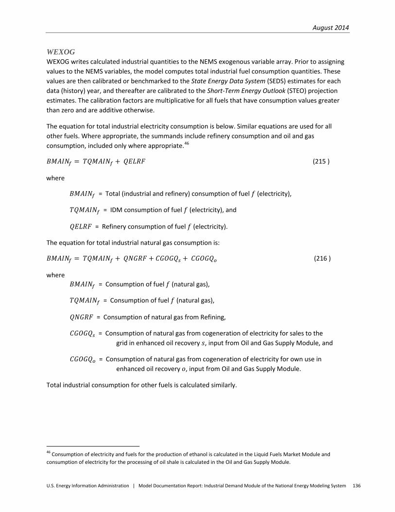
August 2014


WEXOG WEXOG writes calculated industrial quantities to the NEMS exogenous variable array. Prior to assigning values to the NEMS variables, the model computes total industrial fuel consumption quantities. These values are then calibrated or benchmarked to the State Energy Data System (SEDS) estimates for each data (history) year, and thereafter are calibrated to the Short-Term Energy Outlook (STEO) projection estimates. The calibration factors are multiplicative for all fuels that have consumption values greater than zero and are additive otherwise.

The equation for total industrial electricity consumption is below. Similar equations are used for all other fuels. Where appropriate, the summands include refinery consumption and oil and gas consumption, included only where appropriate.46

𝐵𝑀𝐴𝐼𝑁𝑓 = 𝑇𝑄𝑀𝐴𝐼𝑁𝑓 + 𝑄𝐸𝐿𝑅𝐹 (215 )

where

𝐵𝑀𝐴𝐼𝑁𝑓 = Total (industrial and refinery) consumption of fuel 𝑓 (electricity),

𝑇𝑄𝑀𝐴𝐼𝑁𝑓 = IDM consumption of fuel 𝑓 (electricity), and

𝑄𝐸𝐿𝑅𝐹 = Refinery consumption of fuel 𝑓 (electricity).

The equation for total industrial natural gas consumption is:

𝐵𝑀𝐴𝐼𝑁𝑓 = 𝑇𝑄𝑀𝐴𝐼𝑁𝑓 + 𝑄𝑁𝐺𝑅𝐹 + 𝐶𝐺𝑂𝐺𝑄𝑠 + 𝐶𝐺𝑂𝐺𝑄𝑜 (216 )

where 𝐵𝑀𝐴𝐼𝑁𝑓 = Consumption of fuel 𝑓 (natural gas),

𝑇𝑄𝑀𝐴𝐼𝑁𝑓 = Consumption of fuel 𝑓 (natural gas),

𝑄𝑁𝐺𝑅𝐹 = Consumption of natural gas from Refining,

𝐶𝐺𝑂𝐺𝑄𝑠 = Consumption of natural gas from cogeneration of electricity for sales to the grid in enhanced oil recovery 𝑠, input from Oil and Gas Supply Module, and

𝐶𝐺𝑂𝐺𝑄𝑜 = Consumption of natural gas from cogeneration of electricity for own use in enhanced oil recovery 𝑜, input from Oil and Gas Supply Module.

Total industrial consumption for other fuels is calculated similarly.

46 Consumption of electricity and fuels for the production of ethanol is calculated in the Liquid Fuels Market Module and consumption of electricity for the processing of oil shale is calculated in the Oil and Gas Supply Module.

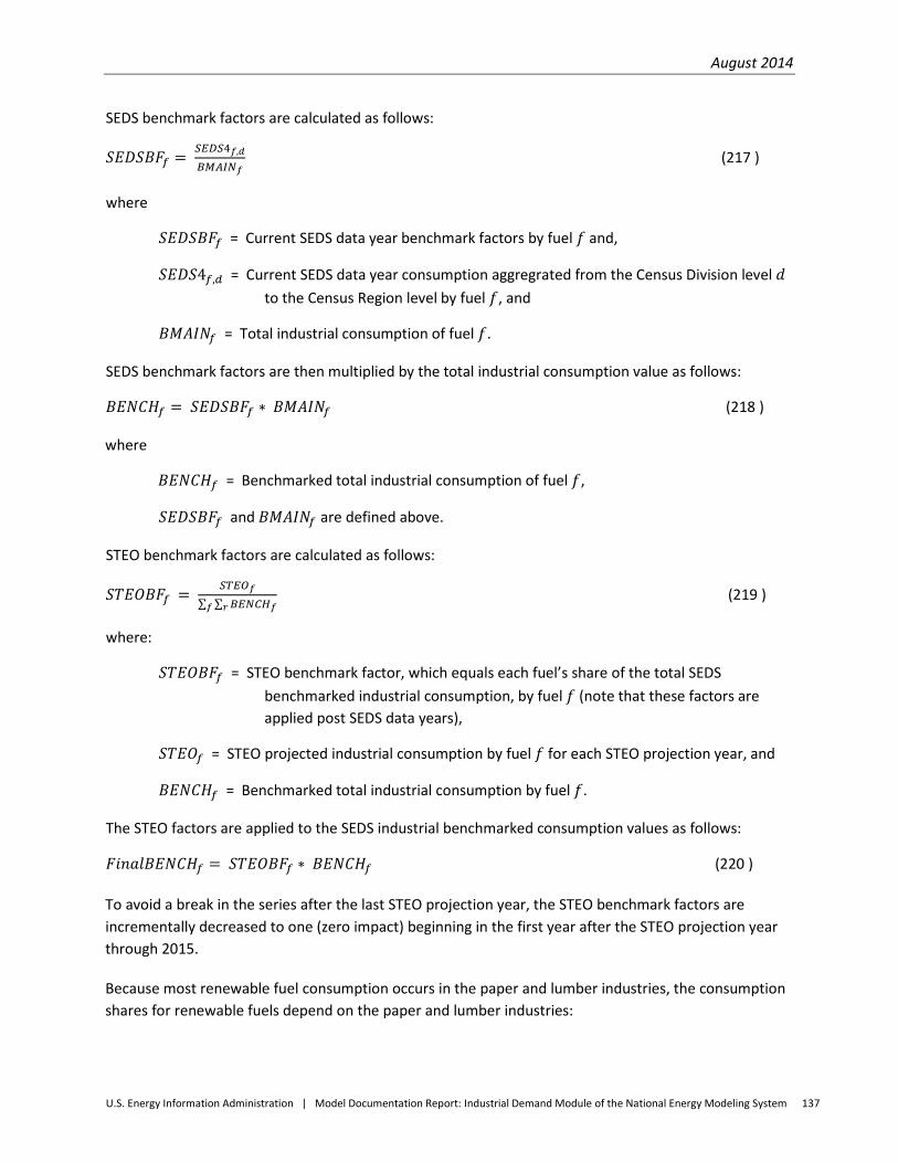
August 2014


SEDS benchmark factors are calculated as follows:

𝑆𝐸𝐷𝑆𝐵𝐹𝑓 = 𝑆𝐸𝐷𝑆4𝑓,𝑑

𝐵𝑀𝐴𝐼𝑁𝑓 (217 )

where

𝑆𝐸𝐷𝑆𝐵𝐹𝑓 = Current SEDS data year benchmark factors by fuel 𝑓 and,

𝑆𝐸𝐷𝑆4𝑓,𝑑 = Current SEDS data year consumption aggregrated from the Census Division level 𝑑 to the Census Region level by fuel 𝑓, and

𝐵𝑀𝐴𝐼𝑁𝑓 = Total industrial consumption of fuel 𝑓.

SEDS benchmark factors are then multiplied by the total industrial consumption value as follows:

𝐵𝐸𝑁𝐶𝐻𝑓 = 𝑆𝐸𝐷𝑆𝐵𝐹𝑓 ∗ 𝐵𝑀𝐴𝐼𝑁𝑓 (218 )

where

𝐵𝐸𝑁𝐶𝐻𝑓 = Benchmarked total industrial consumption of fuel 𝑓,

𝑆𝐸𝐷𝑆𝐵𝐹𝑓 and 𝐵𝑀𝐴𝐼𝑁𝑓 are defined above.

STEO benchmark factors are calculated as follows:

𝑆𝑇𝐸𝑂𝐵𝐹𝑓 = 𝑆𝑇𝐸𝑂𝑓∑ ∑ 𝐵𝐸𝑁𝐶𝐻𝑓𝑟𝑓

(219 )

where:

𝑆𝑇𝐸𝑂𝐵𝐹𝑓 = STEO benchmark factor, which equals each fuel’s share of the total SEDS benchmarked industrial consumption, by fuel 𝑓 (note that these factors are applied post SEDS data years),

𝑆𝑇𝐸𝑂𝑓 = STEO projected industrial consumption by fuel 𝑓 for each STEO projection year, and

𝐵𝐸𝑁𝐶𝐻𝑓 = Benchmarked total industrial consumption by fuel 𝑓.

The STEO factors are applied to the SEDS industrial benchmarked consumption values as follows:

𝐹𝑖𝑛𝑎𝑙𝐵𝐸𝑁𝐶𝐻𝑓 = 𝑆𝑇𝐸𝑂𝐵𝐹𝑓 ∗ 𝐵𝐸𝑁𝐶𝐻𝑓 (220 )

To avoid a break in the series after the last STEO projection year, the STEO benchmark factors are incrementally decreased to one (zero impact) beginning in the first year after the STEO projection year through 2015.

Because most renewable fuel consumption occurs in the paper and lumber industries, the consumption shares for renewable fuels depend on the paper and lumber industries:

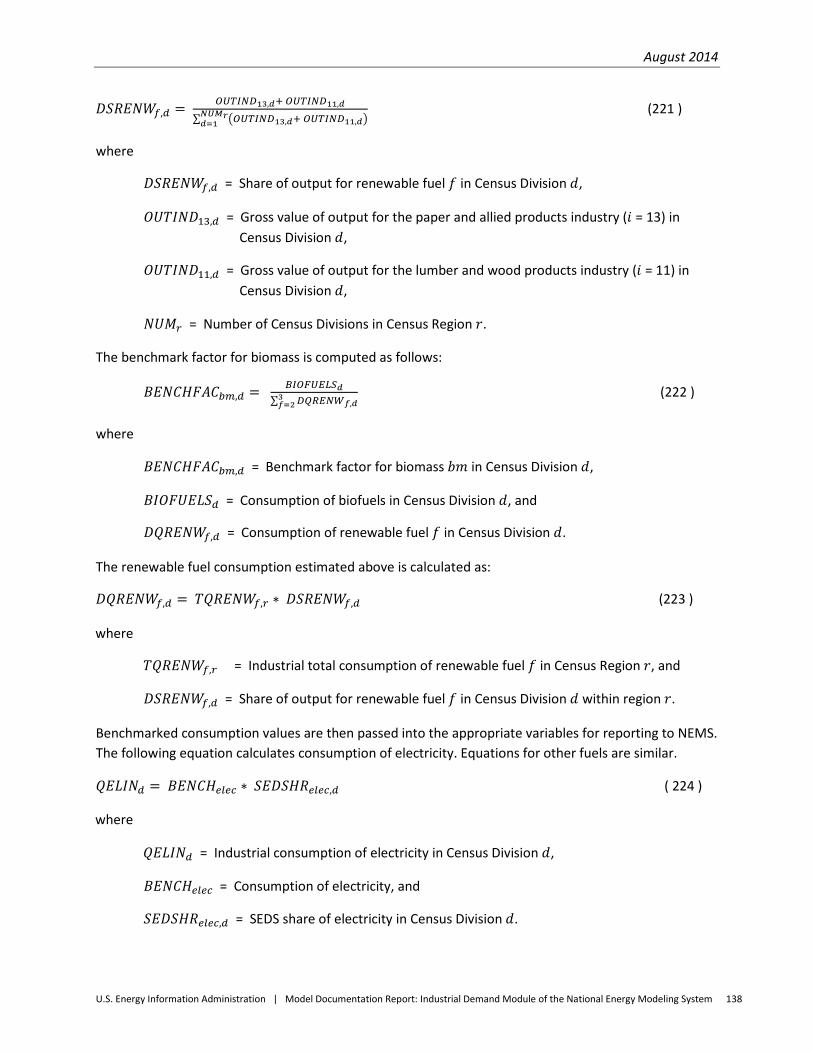
August 2014


𝐷𝑆𝑅𝐸𝑁𝑊𝑓,𝑑 = 𝑂𝑈𝑇𝐼𝑁𝐷13,𝑑+ 𝑂𝑈𝑇𝐼𝑁𝐷11,𝑑

∑ �𝑂𝑈𝑇𝐼𝑁𝐷13,𝑑+ 𝑂𝑈𝑇𝐼𝑁𝐷11,𝑑�𝑁𝑈𝑀𝑟𝑑=1

(221 )

where

𝐷𝑆𝑅𝐸𝑁𝑊𝑓,𝑑 = Share of output for renewable fuel 𝑓 in Census Division 𝑑,

𝑂𝑈𝑇𝐼𝑁𝐷13,𝑑 = Gross value of output for the paper and allied products industry (𝑖 = 13) in Census Division 𝑑,

𝑂𝑈𝑇𝐼𝑁𝐷11,𝑑 = Gross value of output for the lumber and wood products industry (𝑖 = 11) in Census Division 𝑑,

𝑁𝑈𝑀𝑟 = Number of Census Divisions in Census Region 𝑟.

The benchmark factor for biomass is computed as follows:

𝐵𝐸𝑁𝐶𝐻𝐹𝐴𝐶𝑏𝑚,𝑑 = 𝐵𝐼𝑂𝐹𝑈𝐸𝐿𝑆𝑑∑ 𝐷𝑄𝑅𝐸𝑁𝑊𝑓,𝑑3 𝑓=2

(222 )

where

𝐵𝐸𝑁𝐶𝐻𝐹𝐴𝐶𝑏𝑚,𝑑 = Benchmark factor for biomass 𝑏𝑚 in Census Division 𝑑,

𝐵𝐼𝑂𝐹𝑈𝐸𝐿𝑆𝑑 = Consumption of biofuels in Census Division 𝑑, and

𝐷𝑄𝑅𝐸𝑁𝑊𝑓,𝑑 = Consumption of renewable fuel 𝑓 in Census Division 𝑑.

The renewable fuel consumption estimated above is calculated as:

𝐷𝑄𝑅𝐸𝑁𝑊𝑓,𝑑 = 𝑇𝑄𝑅𝐸𝑁𝑊𝑓,𝑟 ∗ 𝐷𝑆𝑅𝐸𝑁𝑊𝑓,𝑑 (223 )

where

𝑇𝑄𝑅𝐸𝑁𝑊𝑓,𝑟 = Industrial total consumption of renewable fuel 𝑓 in Census Region 𝑟, and

𝐷𝑆𝑅𝐸𝑁𝑊𝑓,𝑑 = Share of output for renewable fuel 𝑓 in Census Division 𝑑 within region 𝑟.

Benchmarked consumption values are then passed into the appropriate variables for reporting to NEMS. The following equation calculates consumption of electricity. Equations for other fuels are similar.

𝑄𝐸𝐿𝐼𝑁𝑑 = 𝐵𝐸𝑁𝐶𝐻𝑒𝑙𝑒𝑐 ∗ 𝑆𝐸𝐷𝑆𝐻𝑅𝑒𝑙𝑒𝑐,𝑑 ( 224 )

where

𝑄𝐸𝐿𝐼𝑁𝑑 = Industrial consumption of electricity in Census Division 𝑑,

𝐵𝐸𝑁𝐶𝐻𝑒𝑙𝑒𝑐 = Consumption of electricity, and

𝑆𝐸𝐷𝑆𝐻𝑅𝑒𝑙𝑒𝑐,𝑑 = SEDS share of electricity in Census Division 𝑑.

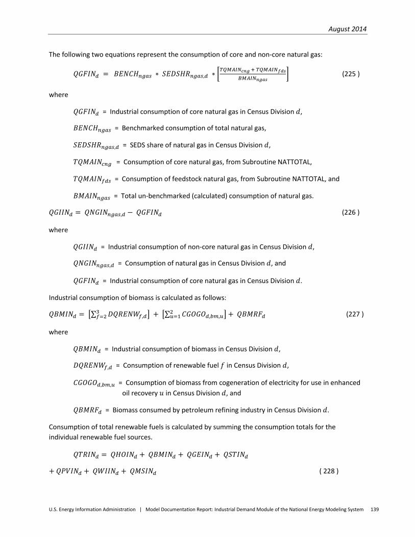
August 2014


The following two equations represent the consumption of core and non-core natural gas:

𝑄𝐺𝐹𝐼𝑁𝑑 = 𝐵𝐸𝑁𝐶𝐻𝑛𝑔𝑎𝑠 ∗ 𝑆𝐸𝐷𝑆𝐻𝑅𝑛𝑔𝑎𝑠,𝑑 ∗ �𝑇𝑄𝑀𝐴𝐼𝑁𝑐𝑛𝑔 + 𝑇𝑄𝑀𝐴𝐼𝑁𝑓𝑑𝑠𝐵𝑀𝐴𝐼𝑁𝑛𝑔𝑎𝑠

� (225 )

where

𝑄𝐺𝐹𝐼𝑁𝑑 = Industrial consumption of core natural gas in Census Division 𝑑,

𝐵𝐸𝑁𝐶𝐻𝑛𝑔𝑎𝑠 = Benchmarked consumption of total natural gas,

𝑆𝐸𝐷𝑆𝐻𝑅𝑛𝑔𝑎𝑠,𝑑 = SEDS share of natural gas in Census Division 𝑑,

𝑇𝑄𝑀𝐴𝐼𝑁𝑐𝑛𝑔 = Consumption of core natural gas, from Subroutine NATTOTAL,

𝑇𝑄𝑀𝐴𝐼𝑁𝑓𝑑𝑠 = Consumption of feedstock natural gas, from Subroutine NATTOTAL, and

𝐵𝑀𝐴𝐼𝑁𝑛𝑔𝑎𝑠 = Total un-benchmarked (calculated) consumption of natural gas.

𝑄𝐺𝐼𝐼𝑁𝑑 = 𝑄𝑁𝐺𝐼𝑁𝑛𝑔𝑎𝑠,𝑑 − 𝑄𝐺𝐹𝐼𝑁𝑑 (226 )

where

𝑄𝐺𝐼𝐼𝑁𝑑 = Industrial consumption of non-core natural gas in Census Division 𝑑,

𝑄𝑁𝐺𝐼𝑁𝑛𝑔𝑎𝑠,𝑑 = Consumption of natural gas in Census Division 𝑑, and

𝑄𝐺𝐹𝐼𝑁𝑑 = Industrial consumption of core natural gas in Census Division 𝑑.

Industrial consumption of biomass is calculated as follows:

𝑄𝐵𝑀𝐼𝑁𝑑 = �∑ 𝐷𝑄𝑅𝐸𝑁𝑊𝑓,𝑑3𝑓=2 � + �∑ 𝐶𝐺𝑂𝐺𝑂𝑑,𝑏𝑚,𝑢

2𝑢=1 �+ 𝑄𝐵𝑀𝑅𝐹𝑑 (227 )

where

𝑄𝐵𝑀𝐼𝑁𝑑 = Industrial consumption of biomass in Census Division 𝑑,

𝐷𝑄𝑅𝐸𝑁𝑊𝑓,𝑑 = Consumption of renewable fuel 𝑓 in Census Division 𝑑,

𝐶𝐺𝑂𝐺𝑂𝑑,𝑏𝑚,𝑢 = Consumption of biomass from cogeneration of electricity for use in enhanced oil recovery 𝑢 in Census Division 𝑑, and

𝑄𝐵𝑀𝑅𝐹𝑑 = Biomass consumed by petroleum refining industry in Census Division 𝑑.

Consumption of total renewable fuels is calculated by summing the consumption totals for the individual renewable fuel sources.

𝑄𝑇𝑅𝐼𝑁𝑑 = 𝑄𝐻𝑂𝐼𝑁𝑑 + 𝑄𝐵𝑀𝐼𝑁𝑑 + 𝑄𝐺𝐸𝐼𝑁𝑑 + 𝑄𝑆𝑇𝐼𝑁𝑑

+ 𝑄𝑃𝑉𝐼𝑁𝑑 + 𝑄𝑊𝐼𝐼𝑁𝑑 + 𝑄𝑀𝑆𝐼𝑁𝑑 ( 228 )

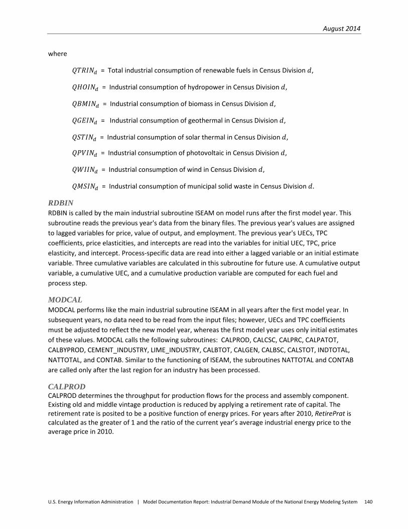
August 2014


where

𝑄𝑇𝑅𝐼𝑁𝑑 = Total industrial consumption of renewable fuels in Census Division 𝑑,

𝑄𝐻𝑂𝐼𝑁𝑑 = Industrial consumption of hydropower in Census Division 𝑑,

𝑄𝐵𝑀𝐼𝑁𝑑 = Industrial consumption of biomass in Census Division 𝑑,

𝑄𝐺𝐸𝐼𝑁𝑑 = Industrial consumption of geothermal in Census Division 𝑑,

𝑄𝑆𝑇𝐼𝑁𝑑 = Industrial consumption of solar thermal in Census Division 𝑑,

𝑄𝑃𝑉𝐼𝑁𝑑 = Industrial consumption of photovoltaic in Census Division 𝑑,

𝑄𝑊𝐼𝐼𝑁𝑑 = Industrial consumption of wind in Census Division 𝑑,

𝑄𝑀𝑆𝐼𝑁𝑑 = Industrial consumption of municipal solid waste in Census Division 𝑑.

RDBIN RDBIN is called by the main industrial subroutine ISEAM on model runs after the first model year. This subroutine reads the previous year's data from the binary files. The previous year's values are assigned to lagged variables for price, value of output, and employment. The previous year's UECs, TPC coefficients, price elasticities, and intercepts are read into the variables for initial UEC, TPC, price elasticity, and intercept. Process-specific data are read into either a lagged variable or an initial estimate variable. Three cumulative variables are calculated in this subroutine for future use. A cumulative output variable, a cumulative UEC, and a cumulative production variable are computed for each fuel and process step.

MODCAL MODCAL performs like the main industrial subroutine ISEAM in all years after the first model year. In subsequent years, no data need to be read from the input files; however, UECs and TPC coefficients must be adjusted to reflect the new model year, whereas the first model year uses only initial estimates of these values. MODCAL calls the following subroutines: CALPROD, CALCSC, CALPRC, CALPATOT, CALBYPROD, CEMENT_INDUSTRY, LIME_INDUSTRY, CALBTOT, CALGEN, CALBSC, CALSTOT, INDTOTAL, NATTOTAL, and CONTAB. Similar to the functioning of ISEAM, the subroutines NATTOTAL and CONTAB are called only after the last region for an industry has been processed.

CALPROD CALPROD determines the throughput for production flows for the process and assembly component. Existing old and middle vintage production is reduced by applying a retirement rate of capital. The retirement rate is posited to be a positive function of energy prices. For years after 2010, RetirePrat is calculated as the greater of 1 and the ratio of the current year’s average industrial energy price to the average price in 2010.

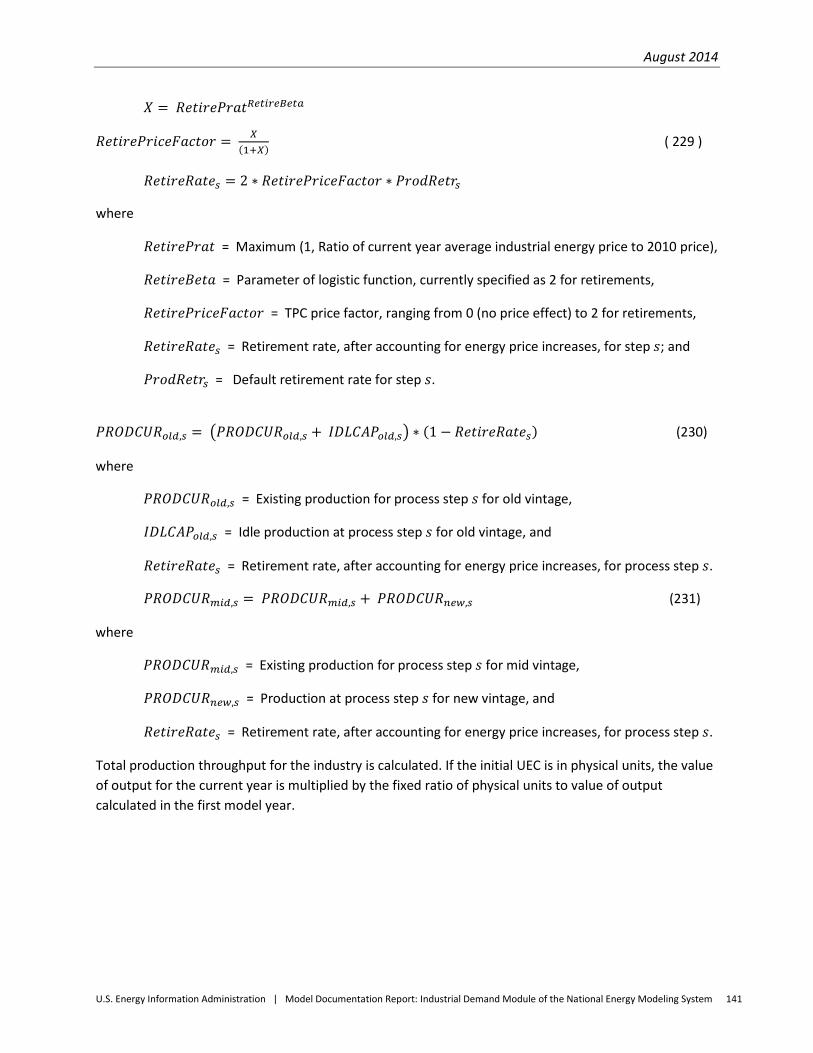
August 2014


𝑋 = 𝑅𝑒𝑡𝑖𝑟𝑒𝑃𝑟𝑎𝑡𝑅𝑒𝑡𝑖𝑟𝑒𝐵𝑒𝑡𝑎

𝑅𝑒𝑡𝑖𝑟𝑒𝑃𝑟𝑖𝑐𝑒𝐹𝑎𝑐𝑡𝑜𝑟 = 𝑋(1+𝑋) ( 229 )

𝑅𝑒𝑡𝑖𝑟𝑒𝑅𝑎𝑡𝑒𝑠 = 2 ∗ 𝑅𝑒𝑡𝑖𝑟𝑒𝑃𝑟𝑖𝑐𝑒𝐹𝑎𝑐𝑡𝑜𝑟 ∗ 𝑃𝑟𝑜𝑑𝑅𝑒𝑡𝑟𝑠

where

𝑅𝑒𝑡𝑖𝑟𝑒𝑃𝑟𝑎𝑡 = Maximum (1, Ratio of current year average industrial energy price to 2010 price),

𝑅𝑒𝑡𝑖𝑟𝑒𝐵𝑒𝑡𝑎 = Parameter of logistic function, currently specified as 2 for retirements,

𝑅𝑒𝑡𝑖𝑟𝑒𝑃𝑟𝑖𝑐𝑒𝐹𝑎𝑐𝑡𝑜𝑟 = TPC price factor, ranging from 0 (no price effect) to 2 for retirements,

𝑅𝑒𝑡𝑖𝑟𝑒𝑅𝑎𝑡𝑒𝑠 = Retirement rate, after accounting for energy price increases, for step 𝑠; and

𝑃𝑟𝑜𝑑𝑅𝑒𝑡𝑟𝑠 = Default retirement rate for step 𝑠.

𝑃𝑅𝑂𝐷𝐶𝑈𝑅𝑜𝑙𝑑,𝑠 = �𝑃𝑅𝑂𝐷𝐶𝑈𝑅𝑜𝑙𝑑,𝑠 + 𝐼𝐷𝐿𝐶𝐴𝑃𝑜𝑙𝑑,𝑠� ∗ (1 − 𝑅𝑒𝑡𝑖𝑟𝑒𝑅𝑎𝑡𝑒𝑠) (230)

where

𝑃𝑅𝑂𝐷𝐶𝑈𝑅𝑜𝑙𝑑,𝑠 = Existing production for process step 𝑠 for old vintage,

𝐼𝐷𝐿𝐶𝐴𝑃𝑜𝑙𝑑,𝑠 = Idle production at process step 𝑠 for old vintage, and

𝑅𝑒𝑡𝑖𝑟𝑒𝑅𝑎𝑡𝑒𝑠 = Retirement rate, after accounting for energy price increases, for process step 𝑠.

𝑃𝑅𝑂𝐷𝐶𝑈𝑅𝑚𝑖𝑑,𝑠 = 𝑃𝑅𝑂𝐷𝐶𝑈𝑅𝑚𝑖𝑑,𝑠 + 𝑃𝑅𝑂𝐷𝐶𝑈𝑅𝑛𝑒𝑤,𝑠 (231)

where

𝑃𝑅𝑂𝐷𝐶𝑈𝑅𝑚𝑖𝑑,𝑠 = Existing production for process step 𝑠 for mid vintage,

𝑃𝑅𝑂𝐷𝐶𝑈𝑅𝑛𝑒𝑤,𝑠 = Production at process step 𝑠 for new vintage, and

𝑅𝑒𝑡𝑖𝑟𝑒𝑅𝑎𝑡𝑒𝑠 = Retirement rate, after accounting for energy price increases, for process step 𝑠.

Total production throughput for the industry is calculated. If the initial UEC is in physical units, the value of output for the current year is multiplied by the fixed ratio of physical units to value of output calculated in the first model year.

August 2014


𝑃𝑅𝑂𝐷𝑋 = 𝑃𝐻𝐷𝑅𝐴𝑇 ∗ 𝑃𝑅𝑂𝐷𝑉𝑋 ( 232 )

where

𝑃𝑅𝑂𝐷𝑋 = Value of output in physical units,

𝑃𝐻𝐷𝑅𝐴𝑇 = Ratio of physical units to value of output (by industry but not region), and

𝑃𝑅𝑂𝐷𝑉𝑋 = Output in dollars.

If the initial UEC is in dollar units, then the current year's value of output is used to determine total production throughput. Total production throughput is calculated by determining new capacity requirements at each process step so as to meet final demand changes and replace retired capacity. This is complicated because retirement rates of some steps differ, as do the process flow rates of old and new capacity. In addition, several process steps may jointly provide output for one or more “downsteps.” The solution to the problem is simplified by formulating the process flow relationships as input-output coefficients as described in the Leontief Input-Output Model (as described in Chiang, Fundamental Methods of Mathematical Economics, pp. 123-131). In this model, the output of a process step can either be a final demand or used as input to another process step. The objective is to determine the mix of old and new productive capacity at each process step such that all final demands are met. In this case, the final demand is the industry output.

The following definitions are provided to illustrate the problem:

A = Input/Output coefficient matrix with final demand as the first column and the production steps as the other columns. The coefficients are the values in the PRODFLOW array, placed in the array according to the IPASTP step definitions,

I = Identity array,

D = Final demand vector, but only the first element in nonzero (𝐷1 is equivalent to 𝑃𝑅𝑂𝐷𝑋), and

X = Vector of productive capacity needed to meet the final demand, based on A and D (X is equivalent to 𝑃𝑅𝑂𝐷𝐶𝑈𝑅).

The input-output model is written as:

(I – A) * X = D ( 233 )

X is obtained by pre-multiplying both sides by the inverse of (I-A):

𝐗 = (𝐈 − 𝐀)−𝟏 ∗ 𝐃 ( 234 )

Since the A coefficients for old and new capacity differ, there are two such arrays: Aold and Anew. The corresponding "technology" matrices (I-Aold) and (I-Anew) will be referred to as IAold and IAnew.

Likewise, Xold and Xnew are distinguished to account for old and new productive capacity. However, to incorporate the retirement calculation, the base year productive capacity will be referred to as Xold and

August 2014


the portion of that capacity that survives to a given year is called Xsurv. The portion that is retired is called Xret. Therefore, total productive capacity (Xtot) is given by:

Xtot = Xsurv + Xnew (235 )

Or

𝐗𝐭𝐨𝐭 = 𝐗𝐨𝐥𝐝 − 𝐗𝐫𝐞𝐭 + 𝐗𝐧𝐞𝐰

Xold is defined in the base year as follows:

𝐈𝐀𝐨𝐥𝐝 ∗ 𝐗𝐨𝐥𝐝 ≡ 𝐃2010

Or (236 )

𝐗𝐨𝐥𝐝 ≡ 𝐈𝐀𝐨𝐥𝐝−𝟏 ∗ 𝐃2010

Xnew is defined as the cumulative capacity additions since the base year.

A set of retirement rates, R, is defined for each producing step. The final demand step need not have a designated retirement rate. Retired capacity is given by:

Xret = Xold ∗ (1 − 𝑅)(𝑌𝑒𝑎𝑟−2010) (237 )

Xsurv = Xold - Xret (238 )

The final demand that can be met by the surviving capacity is given by:

Dold = IAold ∗ Xsurv (239 )

The remaining demand must be met by new capacity, such that the following condition holds:

IAold ∗ Xsurv,year + IAnew ∗ Xnew,year = Dyear (240 )

where, Xnew,year is the cumulative additions to productive capacity since the base year. Xnew,year can be determined by solving the following system:

IAnew ∗ Xnew,year = Dyear – IAold ∗ Xsurv,year (241 )

Therefore,

Xnew,year = IAnew−1 ∗ �Dyear − IAold ∗ Xsurv,year� (242 )

The last equation is used to implement the approach in the model. The solution is found by calling a matrix inversion routine to determine IAnew

-1, followed by calls to intrinsic matrix multiplication functions to solve for Xnew. As a result, the amount of actual code to implement this approach is minimal.

August 2014


CALCSC CALCSC computes Unit Energy Consumption (UEC) for all industries. The current UECs for the old and new vintages are calculated as the product of the previous year’s UEC and a factor that reflects the assumed rate of intensity decline over time and the impact of energy price changes on the assumed decline rate.

𝐸𝑁𝑃𝐼𝑁𝑇𝑣,𝑓,𝑠 = 𝐸𝑁𝑃𝐼𝑁𝑇𝐿𝐴𝐺𝑣,𝑓,𝑠 ∗ (1 + 𝑇𝑃𝐶𝑅𝑎𝑡𝑒𝑣) (243 )

where

𝐸𝑁𝑃𝐼𝑁𝑇𝑣,𝑓,𝑠 = UEC of process step 𝑠 for fuel 𝑓 and vintage 𝑣,

𝐸𝑁𝑃𝐼𝑁𝑇𝐿𝐴𝐺𝑣,𝑓,𝑠 = Lagged UEC of process step 𝑠 for fuel 𝑓 and vintage 𝑣, and

𝑇𝑃𝐶𝑅𝑎𝑡𝑒𝑣 = Energy intensity decline rate for vintage 𝑣 after accounting for the impact of increased energy prices.

TPCRatev is calculated using the following relationships when TPCPrat is greater than 1.0. Otherwise, the default value for the intensity decline rate is used, BCSCv,f,s.


𝑇𝑃𝐶𝑃𝑟𝑖𝑐𝑒𝐹𝑎𝑐𝑡𝑜𝑟 = 𝑋(1+𝑋) (244 )

𝑇𝑃𝐶𝑅𝑎𝑡𝑒𝑣 = 2 ∗ 𝑇𝑃𝐶𝑃𝑟𝑖𝑐𝑒𝐹𝑎𝑐𝑡𝑜𝑟 ∗ 𝐵𝐶𝑆𝐶𝑣,𝑓,𝑠

where

𝑇𝑃𝐶𝑃𝑟𝑎𝑡 = Ratio of current year average industrial energy pruce to 2010 price,

𝑇𝑃𝐶𝐵𝑒𝑡𝑎 = Parameter of logistic function, currently specified as 4,

𝑇𝑃𝐶𝑃𝑟𝑖𝑐𝑒𝐹𝑎𝑐𝑡𝑜𝑟 = TPC price factor, ranging from 0 (no price effect) to 2 for 𝐸𝑁𝑃𝐼𝑁𝑇, and

𝐵𝐶𝑆𝐶𝑣,𝑓,𝑠 = Default intensity rate for old and new vintage 𝑣 for fuel 𝑓 and step 𝑠.

𝑇𝑃𝐶𝑅𝑎𝑡𝑒𝑣 is defined above.

The UEC for middle vintage is calculated as the ratio of cumulative UEC to cumulative production for all process steps and industries, i.e., the weighted average UEC, as follows:

𝐸𝑁𝑃𝐼𝑁𝑇𝑚𝑖𝑑,𝑓,𝑠 = 𝑆𝑈𝑀𝑃𝐼𝑁𝑇𝑓,𝑠

𝐶𝑈𝑀𝑃𝑅𝑂𝐷𝑛𝑒𝑤,𝑠 (245 )

where

𝐸𝑁𝑃𝐼𝑁𝑇𝑚𝑖𝑑,𝑓,𝑠 = UEC of process step 𝑠 for fuel 𝑓 at middle vintage,

𝑆𝑈𝑀𝑃𝐼𝑁𝑇𝑓,𝑠 = Cumulative UEC of process step 𝑠 for fuel 𝑓, and

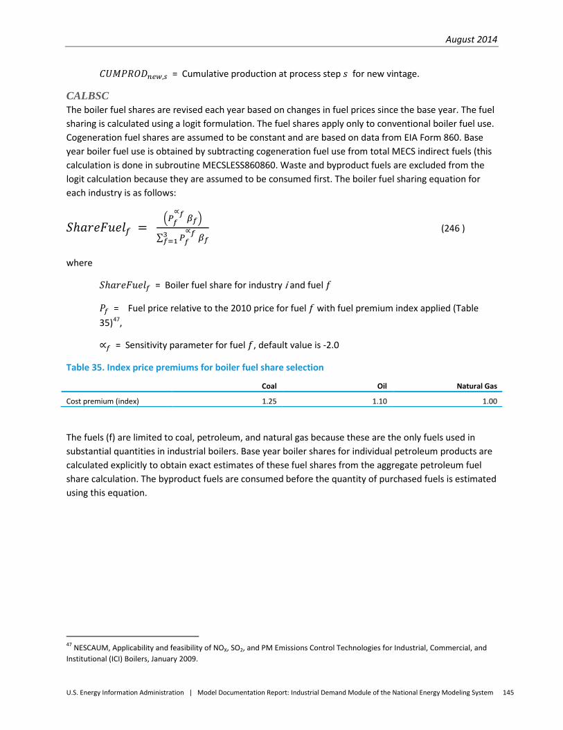
August 2014


𝐶𝑈𝑀𝑃𝑅𝑂𝐷𝑛𝑒𝑤,𝑠 = Cumulative production at process step 𝑠 for new vintage.

CALBSC The boiler fuel shares are revised each year based on changes in fuel prices since the base year. The fuel sharing is calculated using a logit formulation. The fuel shares apply only to conventional boiler fuel use. Cogeneration fuel shares are assumed to be constant and are based on data from EIA Form 860. Base year boiler fuel use is obtained by subtracting cogeneration fuel use from total MECS indirect fuels (this calculation is done in subroutine MECSLESS860860. Waste and byproduct fuels are excluded from the logit calculation because they are assumed to be consumed first. The boiler fuel sharing equation for each industry is as follows:

𝑆ℎ𝑎𝑟𝑒𝐹𝑢𝑒𝑙𝑓 = �𝑃𝑓

∝𝑓 𝛽𝑓�

∑ 𝑃𝑓∝𝑓3

𝑓=1 𝛽𝑓 (246 )

where

𝑆ℎ𝑎𝑟𝑒𝐹𝑢𝑒𝑙𝑓 = Boiler fuel share for industry i and fuel 𝑓

𝑃𝑓 = Fuel price relative to the 2010 price for fuel 𝑓 with fuel premium index applied (Table 35)47,

∝𝑓 = Sensitivity parameter for fuel 𝑓, default value is -2.0

Table 35. Index price premiums for boiler fuel share selection

Coal Oil Natural Gas

Cost premium (index) 1.25 1.10 1.00

The fuels (f) are limited to coal, petroleum, and natural gas because these are the only fuels used in substantial quantities in industrial boilers. Base year boiler shares for individual petroleum products are calculated explicitly to obtain exact estimates of these fuel shares from the aggregate petroleum fuel share calculation. The byproduct fuels are consumed before the quantity of purchased fuels is estimated using this equation.

47 NESCAUM, Applicability and feasibility of NOX, SO2, and PM Emissions Control Technologies for Industrial, Commercial, and Institutional (ICI) Boilers, January 2009.

August 2014


Appendix A. Model Abstract

Model name: Industrial Demand Module

Model acronym: IDM

Description: The Industrial Demand Module is based upon economic and engineering relationships that model industrial sector energy consumption at the Census Division level of detail. The seven most energy-intensive industries are modeled at the detailed process step level and eight other industries are modeled at a less-detailed level. The IDM incorporates three components: buildings; process and assembly; and boiler, steam, and cogeneration.

Purpose of the model: As a component of the National Energy Modeling System integrated modeling tool, the IDM generates long-term projections of industrial sector energy consumption. The IDM facilitates policy analysis of energy markets, technological development, environmental issues, and regulatory development as they impact industrial sector energy consumption.

Most recent model update: October 2013.

Part of another model: National Energy Modeling System (NEMS)

Model interfaces: The Industrial Demand Module receives inputs from the Electricity Market Module, Natural Gas Transmission and Distribution Module, Oil and Gas Supply Module, Renewable Fuels Module, Macroeconomic Activity Module (MAM), Transportation Demand Module (TDM), Commercial Demand Module (CDM), and Liquid Fuels Market Module (LFMM).

Official model representatives: Kelly Perl (202)586-1743 [email protected] Office of Energy Analysis, Office of Energy Consumption and Efficiency Analysis EI-32 1000 Independence Avenue, SW Washington, DC 20585

mailto:[email protected]

August 2014


Documentation: Model Documentation Report: Industrial Demand Module of the National Energy Modeling System, August 2014.

Archive media and installation manual(s): The model is archived as part of the National Energy Modeling System production runs used to generate AEO2014.

Energy system described: Domestic industrial sector energy consumption.

Coverage: Geographic: Nine Census Divisions: New England, Middle Atlantic, East North Central, West North Central, South Atlantic, East South Central, West South Central, Mountain, and Pacific.

Time Unit/Frequency: Annual, 2010 through 2040.

Modeling features: Structure: 15 manufacturing and 6 non-manufacturing industries. The manufacturing industries are further classified as energy-intensive or non-energy-intensive industries.

Each industry is modeled as three separate but interrelated components consisting of the process/assembly component (PA), the buildings component (BLD), and the boiler/steam/cogeneration component (BSC).

Modeling Technique: The energy-intensive industries are modeled either through the use of a detailed process flow with technology diffusion or end-use accounting procedure. The remaining industries use the same general procedure but do not include a detailed process flow.

Non-DOE input sources: Historical Dollar Value of Shipments in the Industrial Sector

Energy Expenditures in the Agriculture and Construction sectors

Energy Consumption in the Mining sector

DOE input sources: Form EIA-923 and predecessor forms: Annual Electric Generator Report

Electricity generation, total and by prime mover

Electricity generation for own use and sales

Capacity utilization

Manufacturing Energy Consumption Survey 2010, March 2013

August 2014


State Energy Data System 2011, June 2013

Monthly Energy Review, (annual data 2012) September 2013

Computing environment: Hardware Used: Intel Xeon CPU

Operating System: Microsoft Windows 7

Language/Software Used: Intel Visual Fortran 11.1

Estimated Run Time: less than one minute for a 2010-2040 run in non-iterating, stand-alone mode.

Special Features: None

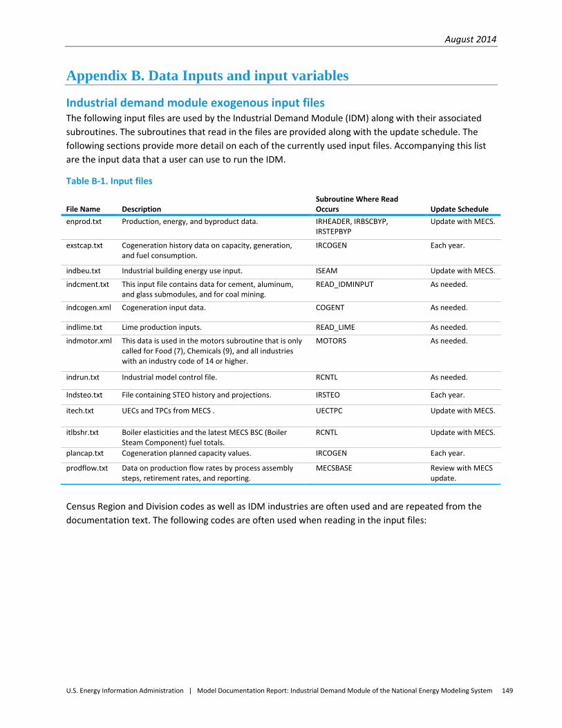
August 2014


Appendix B. Data Inputs and input variables

Industrial demand module exogenous input files The following input files are used by the Industrial Demand Module (IDM) along with their associated subroutines. The subroutines that read in the files are provided along with the update schedule. The following sections provide more detail on each of the currently used input files. Accompanying this list are the input data that a user can use to run the IDM.

Table B-1. Input files

File Name Description Subroutine Where Read Occurs Update Schedule

enprod.txt Production, energy, and byproduct data. IRHEADER, IRBSCBYP, IRSTEPBYP

Update with MECS.

exstcap.txt Cogeneration history data on capacity, generation, and fuel consumption.

IRCOGEN Each year.

indbeu.txt Industrial building energy use input. ISEAM Update with MECS.

indcment.txt This input file contains data for cement, aluminum, and glass submodules, and for coal mining.

READ_IDMINPUT As needed.

indcogen.xml Cogeneration input data. COGENT As needed.

indlime.txt Lime production inputs. READ_LIME As needed.

indmotor.xml This data is used in the motors subroutine that is only called for Food (7), Chemicals (9), and all industries with an industry code of 14 or higher.

MOTORS As needed.

indrun.txt Industrial model control file. RCNTL As needed.

Indsteo.txt File containing STEO history and projections. IRSTEO Each year.

itech.txt UECs and TPCs from MECS . UECTPC Update with MECS.

itlbshr.txt Boiler elasticities and the latest MECS BSC (Boiler Steam Component) fuel totals.

RCNTL Update with MECS.

plancap.txt Cogeneration planned capacity values. IRCOGEN Each year.

prodflow.txt Data on production flow rates by process assembly steps, retirement rates, and reporting.

MECSBASE Review with MECS update.

Census Region and Division codes as well as IDM industries are often used and are repeated from the documentation text. The following codes are often used when reading in the input files:

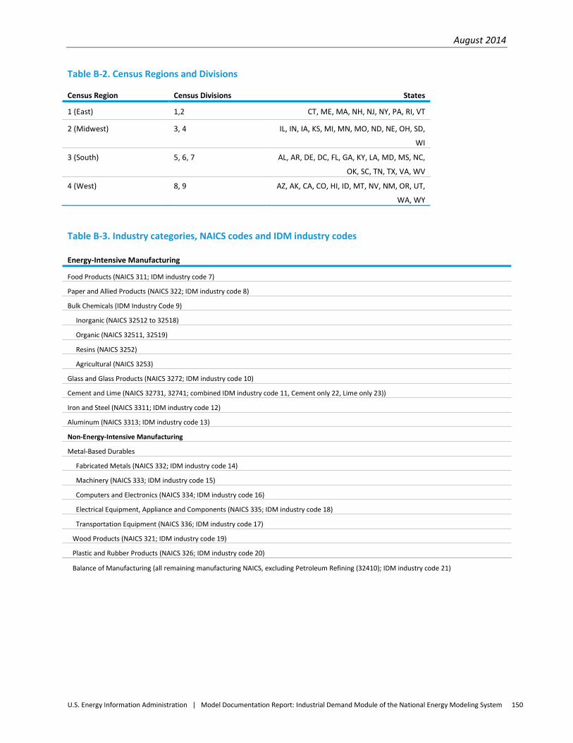
August 2014


Table B-2. Census Regions and Divisions

Census Region Census Divisions States 1 (East) 1,2 CT, ME, MA, NH, NJ, NY, PA, RI, VT

2 (Midwest) 3, 4 IL, IN, IA, KS, MI, MN, MO, ND, NE, OH, SD,

WI

3 (South) 5, 6, 7 AL, AR, DE, DC, FL, GA, KY, LA, MD, MS, NC,

OK, SC, TN, TX, VA, WV

4 (West) 8, 9 AZ, AK, CA, CO, HI, ID, MT, NV, NM, OR, UT,

WA, WY

Table B-3. Industry categories, NAICS codes and IDM industry codes

Energy-Intensive Manufacturing

Food Products (NAICS 311; IDM industry code 7)

Paper and Allied Products (NAICS 322; IDM industry code 8)

Bulk Chemicals (IDM Industry Code 9)

Inorganic (NAICS 32512 to 32518)

Organic (NAICS 32511, 32519)

Resins (NAICS 3252)

Agricultural (NAICS 3253)

Glass and Glass Products (NAICS 3272; IDM industry code 10)

Cement and Lime (NAICS 32731, 32741; combined IDM industry code 11, Cement only 22, Lime only 23))

Iron and Steel (NAICS 3311; IDM industry code 12)

Aluminum (NAICS 3313; IDM industry code 13)

Non-Energy-Intensive Manufacturing

Metal-Based Durables

Fabricated Metals (NAICS 332; IDM industry code 14)

Machinery (NAICS 333; IDM industry code 15)

Computers and Electronics (NAICS 334; IDM industry code 16)

Electrical Equipment, Appliance and Components (NAICS 335; IDM industry code 18)

Transportation Equipment (NAICS 336; IDM industry code 17)

Wood Products (NAICS 321; IDM industry code 19)

Plastic and Rubber Products (NAICS 326; IDM industry code 20)

Balance of Manufacturing (all remaining manufacturing NAICS, excluding Petroleum Refining (32410); IDM industry code 21)

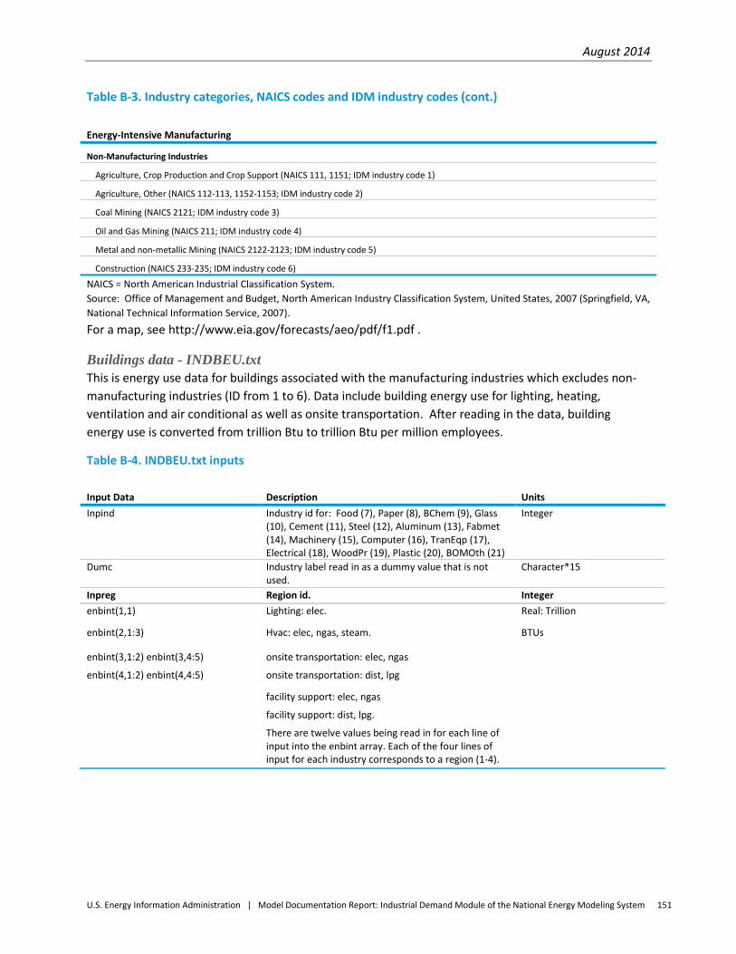
August 2014


Table B-3. Industry categories, NAICS codes and IDM industry codes (cont.)

For a map, see http://www.eia.gov/forecasts/aeo/pdf/f1.pdf .

Buildings data - INDBEU.txt This is energy use data for buildings associated with the manufacturing industries which excludes non-manufacturing industries (ID from 1 to 6). Data include building energy use for lighting, heating, ventilation and air conditional as well as onsite transportation. After reading in the data, building energy use is converted from trillion Btu to trillion Btu per million employees.

Table B-4. INDBEU.txt inputs

Input Data Description Units Inpind Industry id for: Food (7), Paper (8), BChem (9), Glass

(10), Cement (11), Steel (12), Aluminum (13), Fabmet (14), Machinery (15), Computer (16), TranEqp (17), Electrical (18), WoodPr (19), Plastic (20), BOMOth (21)

Integer

Dumc Industry label read in as a dummy value that is not used.

Character*15

Inpreg Region id. Integer enbint(1,1) Lighting: elec. Real: Trillion

enbint(2,1:3) Hvac: elec, ngas, steam. BTUs

enbint(3,1:2) enbint(3,4:5) onsite transportation: elec, ngas

enbint(4,1:2) enbint(4,4:5) onsite transportation: dist, lpg

facility support: elec, ngas

facility support: dist, lpg.

There are twelve values being read in for each line of input into the enbint array. Each of the four lines of input for each industry corresponds to a region (1-4).

Energy-Intensive Manufacturing

Non-Manufacturing Industries

Agriculture, Crop Production and Crop Support (NAICS 111, 1151; IDM industry code 1)

Agriculture, Other (NAICS 112-113, 1152-1153; IDM industry code 2)

Coal Mining (NAICS 2121; IDM industry code 3)

Oil and Gas Mining (NAICS 211; IDM industry code 4)

Metal and non-metallic Mining (NAICS 2122-2123; IDM industry code 5)

Construction (NAICS 233-235; IDM industry code 6)

NAICS = North American Industrial Classification System. Source: Office of Management and Budget, North American Industry Classification System, United States, 2007 (Springfield, VA, National Technical Information Service, 2007).

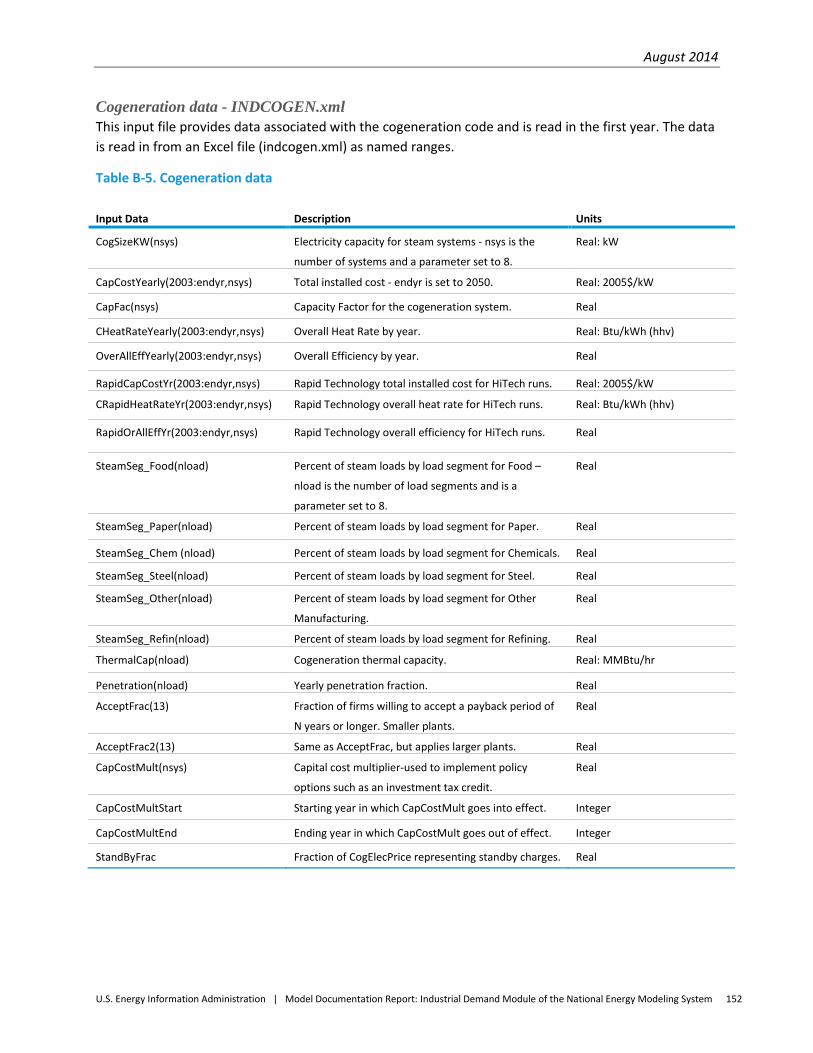
August 2014


Cogeneration data - INDCOGEN.xml This input file provides data associated with the cogeneration code and is read in the first year. The data is read in from an Excel file (indcogen.xml) as named ranges.

Table B-5. Cogeneration data

Input Data Description Units

CogSizeKW(nsys) Electricity capacity for steam systems - nsys is the

number of systems and a parameter set to 8.

Real: kW

CapCostYearly(2003:endyr,nsys) Total installed cost - endyr is set to 2050. Real: 2005$/kW

CapFac(nsys) Capacity Factor for the cogeneration system. Real

CHeatRateYearly(2003:endyr,nsys) Overall Heat Rate by year. Real: Btu/kWh (hhv)

OverAllEffYearly(2003:endyr,nsys) Overall Efficiency by year. Real

RapidCapCostYr(2003:endyr,nsys) Rapid Technology total installed cost for HiTech runs. Real: 2005$/kW

CRapidHeatRateYr(2003:endyr,nsys) Rapid Technology overall heat rate for HiTech runs. Real: Btu/kWh (hhv)

RapidOrAllEffYr(2003:endyr,nsys) Rapid Technology overall efficiency for HiTech runs. Real

SteamSeg_Food(nload) Percent of steam loads by load segment for Food –

nload is the number of load segments and is a

parameter set to 8.

Real

SteamSeg_Paper(nload) Percent of steam loads by load segment for Paper. Real

SteamSeg_Chem (nload) Percent of steam loads by load segment for Chemicals. Real

SteamSeg_Steel(nload) Percent of steam loads by load segment for Steel. Real

SteamSeg_Other(nload) Percent of steam loads by load segment for Other

Manufacturing.

Real

SteamSeg_Refin(nload) Percent of steam loads by load segment for Refining. Real

ThermalCap(nload) Cogeneration thermal capacity. Real: MMBtu/hr

Penetration(nload) Yearly penetration fraction. Real

AcceptFrac(13) Fraction of firms willing to accept a payback period of

N years or longer. Smaller plants.

Real

AcceptFrac2(13) Same as AcceptFrac, but applies larger plants. Real

CapCostMult(nsys) Capital cost multiplier-used to implement policy

options such as an investment tax credit.

Real

CapCostMultStart Starting year in which CapCostMult goes into effect. Integer

CapCostMultEnd Ending year in which CapCostMult goes out of effect. Integer

StandByFrac Fraction of CogElecPrice representing standby charges. Real

August 2014


Higher heating value (hhv)—Gross heating value—equal to the total heat obtained from combustion of a specified amount of fuel and its stoichiometrically correct amount of air, both being at 60°F when combustion starts, and after the combustion products are cooled. HHV assumes all the water component is in liquid state at the end of combustion.

Energy and production data file - ENPROD.txt There are three separate sets of data in this file that are read in by the following three separate subroutines:

• IRHEADER: Reads industry and region identifier numbers, base year values of output, physical to dollar output conversion factors, and base year steam demand. This input is required.

• IRBSCBYP: Reads byproduct fuel information for the boiler/steam/cogeneration component. These data consist of fuel identifier numbers and steam intensity values. This input is not required.

• IRSTEPBYP: Reads byproduct data for process and assembly component. These data consist of fuel identifier numbers and heat intensity values. This input is not required. The step name is limited to 8 characters since this name is placed in an 8 character matrix for steps in the enprod.txt file. Otherwise, the limit is 24 characters. The step names from the prodflow.txt file are used.

The code that reads in the IRHEADER data calculates the ratio of physical output to 2010 (most recent MECS data) value of shipments for pulp and paper, glass, cement, steel and aluminum industries. This constant ratio is applied to value of shipments for subsequent years.

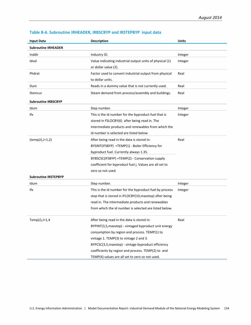
August 2014


Table B-6. Subroutine IRHEADER, IRBSCBYP and IRSTEPBYP input data


Subroutine IRHEADER

Inddir Industry ID. Integer

Idval Value indicating industrial output units of physical (1)

or dollar value (2).

Integer

Phdrat Factor used to convert industrial output from physical

to dollar units.

Real

Dum Reads in a dummy value that is not currently used. Real

Stemcur Steam demand from process/assembly and buildings. Real

Subroutine IRBSCBYP

Idum Step number. Integer

Ifx This is the id number for the byproduct fuel that is

stored in FSLOCBY(6) after being read in. The

intermediate products and renewables from which the

id number is selected are listed below.

Integer

(temp(J),J=1,2) After being read in the data is stored in:

BYSINT(IFSBYP) =TEMP(1) - Boiler Efficiency for

byproduct fuel. Currently always 1.35.

Real

BYBSCSC(IFSBYP) =TEMP(2) - Conservation supply

coefficient for byproduct fuel j. Values are all set to

zero so not used.

Subroutine IRSTEPBYP

Idum Step number. Integer

Ifx This is the id number for the byproduct fuel by process

step that is stored in IFLOCBY(10,maxstep) after being

read in. The intermediate products and renewables

from which the id number is selected are listed below.

Integer

Temp(J),J=1,4 After being read in the data is stored in:

BYPINT(3,5,maxstep) - vintaged byproduct unit energy

consumption by region and process. TEMP(1) to

vintage 1. TEMP(3) to vintage 2 and 3.

BYPCSC(3,5,maxstep) - vintage byproduct efficiency

coefficients by region and process. TEMP(2) to and

TEMP(4) values are all set to zero so not used.

Real

August 2014


THE INTERMEDIATE PRODUCTS QUANTITY ARRAY: QTYINTR(6,5)

1. STEAM (31) 2. COKE OVEN GAS (32) - currently used in enprod.txt 3. BLAST FURNACE GAS (33) – currently used in enprod.txt 4. OTHER BYPRODUCT GAS (34) 5. WASTE HEAT (35) – currently used in enprod.txt 6. COKE (36)

THE RENEWABLES QUANTITY ARRAY: QTYRENW(8,5)

1. HYDROPOWER (41) 2. BIOMASS-WOOD (42) – currently used in enprod.txt 3. BIOMASS-PULPING LIQUOR (43) – currently used in enprod.txt 4. GEOTHERMAL (44) 5. SOLAR (45) 6. PHOTOVOLTAIC (46) 7. WIND (47) 8. MUNICIPAL SOLID WASTE (48)

Industrial model control file - INDRUN.txt These values generally do not change. However, when running the Frozen Technology case the FRSTECH value is changed to 1. When running the High Technology case the HITECH value is changed to 1. Unless otherwise indicated the value used in the table is the default value.

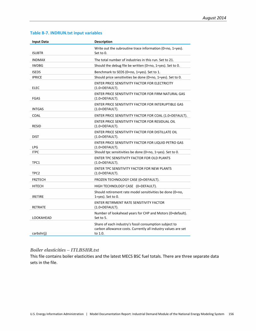
August 2014


Table B-7. INDRUN.txt input variables

Input Data Description

ISUBTR Write out the subroutine trace information (0=no, 1=yes). Set to 0.

INDMAX The total number of industries in this run. Set to 21. IWDBG Should the debug file be written (0=no, 1=yes). Set to 0.

ISEDS Benchmark to SEDS (0=no, 1=yes). Set to 1. IPRICE Should price sensitivities be done (0=no, 1=yes). Set to 0.

ELEC ENTER PRICE SENSITIVITY FACTOR FOR ELECTRICITY (1.0=DEFAULT).

FGAS ENTER PRICE SENSITIVITY FACTOR FOR FIRM NATURAL GAS (1.0=DEFAULT).

INTGAS ENTER PRICE SENSITIVITY FACTOR FOR INTERUPTIBLE GAS (1.0=DEFAULT).

COAL ENTER PRICE SENSITIVITY FACTOR FOR COAL (1.0=DEFAULT).

RESID ENTER PRICE SENSITIVITY FACTOR FOR RESIDUAL OIL (1.0=DEFAULT).

DIST ENTER PRICE SENSITIVITY FACTOR FOR DISTILLATE OIL (1.0=DEFAULT).

LPG ENTER PRICE SENSITIVITY FACTOR FOR LIQUID PETRO GAS (1.0=DEFAULT).

ITPC Should tpc sensitivities be done (0=no, 1=yes). Set to 0.

TPC1 ENTER TPC SENSITIVITY FACTOR FOR OLD PLANTS (1.0=DEFAULT).

TPC2 ENTER TPC SENSITIVITY FACTOR FOR NEW PLANTS (1.0=DEFAULT).

FRZTECH FROZEN TECHNOLOGY CASE (0=DEFAULT).

HITECH HIGH TECHNOLOGY CASE (0=DEFAULT).

IRETIRE Should retirement rate model sensitivities be done (0=no, 1=yes). Set to 0.

RETRATE ENTER RETIRMENT RATE SENSITIVITY FACTOR (1.0=DEFAULT).

LOOKAHEAD Number of lookahead years for CHP and Motors (0=default). Set to 5.

carbshr(j)

Share of each industry's fossil consumption subject to carbon allowance costs. Currently all industry values are set to 1.0.

Boiler elasticities – ITLBSHR.txt This file contains boiler elasticities and the latest MECS BSC fuel totals. There are three separate data sets in the file.

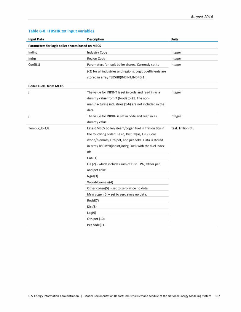
August 2014


Table B-8. ITBSHR.txt input variables


Parameters for logit boiler shares based on MECS

Indint Industry Code Integer

Indrg Region Code Integer

Coeff(1) Parameters for logit boiler shares. Currently set to Integer

(-2) for all industries and regions. Logic coefficients are

stored in array TLBSHR(INDINT,INDRG,1).

Boiler Fuels from MECS

j The value for INDINT is set in code and read in as a

dummy value from 7 (food) to 21. The non-

manufacturing industries (1-6) are not included in the

data.

Integer

j The value for INDRG is set in code and read in as

dummy value.

Integer

Temp(k),k=1,8 Latest MECS boiler/steam/cogen fuel in Trillion Btu in

the following order: Resid, Dist, Ngas, LPG, Coal,

wood/biomass, Oth pet, and pet coke. Data is stored

in array BSCIBYR(indint,indrg,Fuel) with the fuel index

of:

Real: Trillion Btu

Coal(1)

Oil (2) - which includes sum of Dist, LPG, Other pet,

and pet coke.

Ngas(3)

Wood/biomass(4)

Other cogen(5) - set to zero since no data.

Msw cogen(6) – set to zero since no data.

Resid(7)

Dist(8)

Lpg(9)

Oth pet (10)

Pet code(11)

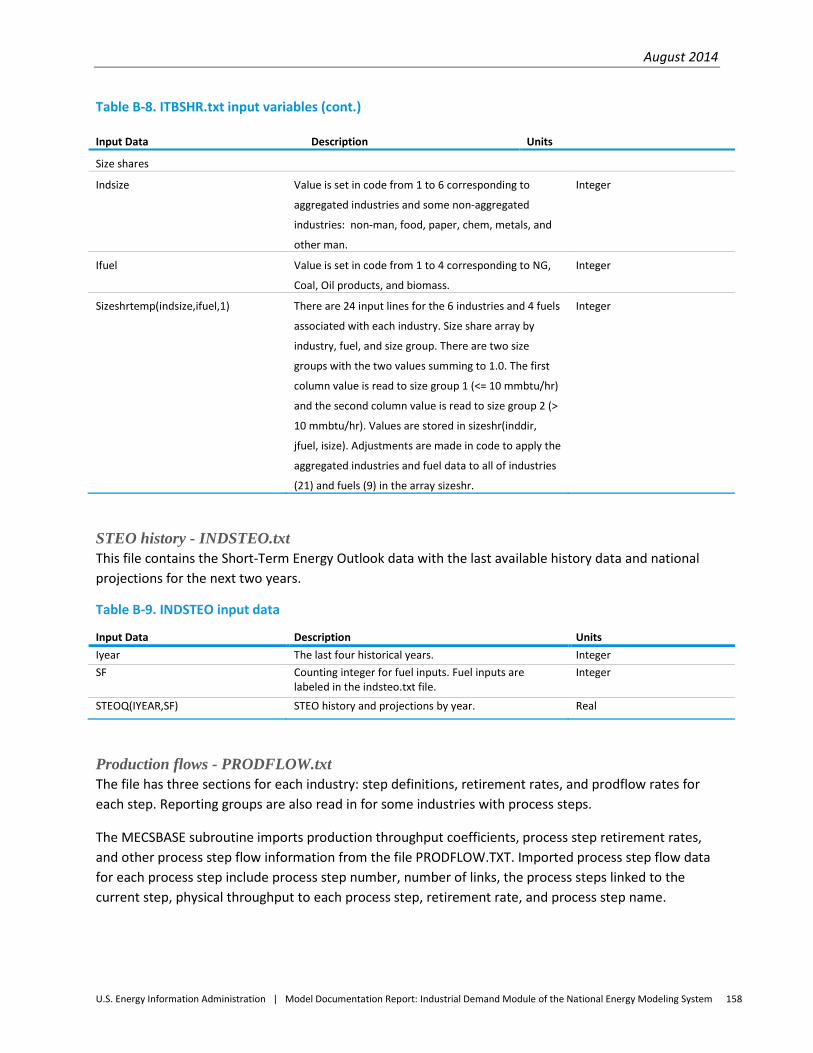
August 2014


Table B-8. ITBSHR.txt input variables (cont.)


Size shares

Indsize Value is set in code from 1 to 6 corresponding to

aggregated industries and some non-aggregated

industries: non-man, food, paper, chem, metals, and

other man.

Integer

Ifuel Value is set in code from 1 to 4 corresponding to NG,

Coal, Oil products, and biomass.

Integer

Sizeshrtemp(indsize,ifuel,1) There are 24 input lines for the 6 industries and 4 fuels

associated with each industry. Size share array by

industry, fuel, and size group. There are two size

groups with the two values summing to 1.0. The first

column value is read to size group 1 (<= 10 mmbtu/hr)

and the second column value is read to size group 2 (>

10 mmbtu/hr). Values are stored in sizeshr(inddir,

jfuel, isize). Adjustments are made in code to apply the

aggregated industries and fuel data to all of industries

(21) and fuels (9) in the array sizeshr.

Integer

STEO history - INDSTEO.txt This file contains the Short-Term Energy Outlook data with the last available history data and national projections for the next two years.

Table B-9. INDSTEO input data

Input Data Description Units Iyear The last four historical years. Integer SF Counting integer for fuel inputs. Fuel inputs are

labeled in the indsteo.txt file. Integer

STEOQ(IYEAR,SF) STEO history and projections by year. Real

Production flows - PRODFLOW.txt The file has three sections for each industry: step definitions, retirement rates, and prodflow rates for each step. Reporting groups are also read in for some industries with process steps.

The MECSBASE subroutine imports production throughput coefficients, process step retirement rates, and other process step flow information from the file PRODFLOW.TXT. Imported process step flow data for each process step include process step number, number of links, the process steps linked to the current step, physical throughput to each process step, retirement rate, and process step name.

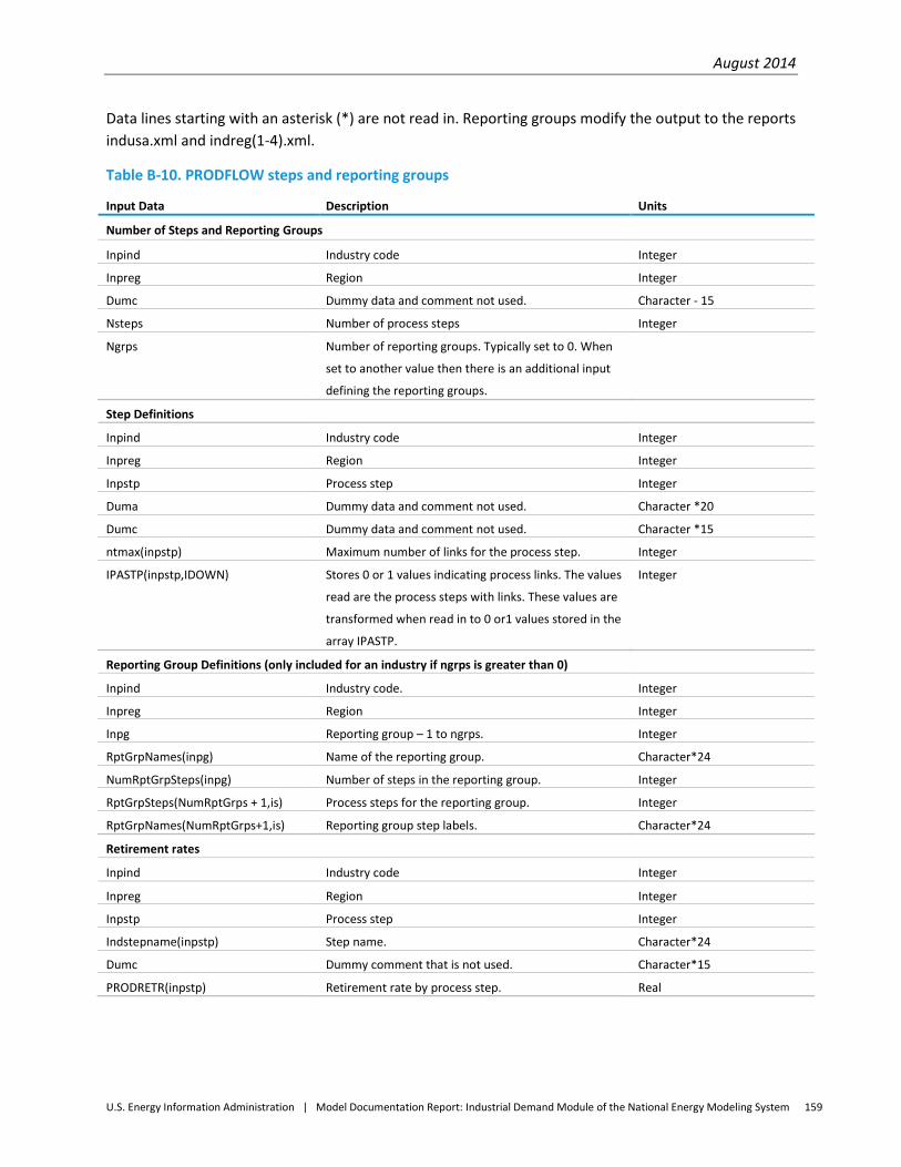
August 2014


Data lines starting with an asterisk (*) are not read in. Reporting groups modify the output to the reports indusa.xml and indreg(1-4).xml.

Table B-10. PRODFLOW steps and reporting groups


Number of Steps and Reporting Groups

Inpind Industry code Integer

Inpreg Region Integer

Dumc Dummy data and comment not used. Character - 15

Nsteps Number of process steps Integer

Ngrps Number of reporting groups. Typically set to 0. When

set to another value then there is an additional input

defining the reporting groups.

Step Definitions



Inpstp Process step Integer

Duma Dummy data and comment not used. Character *20

Dumc Dummy data and comment not used. Character *15

ntmax(inpstp) Maximum number of links for the process step. Integer

IPASTP(inpstp,IDOWN) Stores 0 or 1 values indicating process links. The values

read are the process steps with links. These values are

transformed when read in to 0 or1 values stored in the

array IPASTP.

Integer

Reporting Group Definitions (only included for an industry if ngrps is greater than 0)

Inpind Industry code. Integer


Inpg Reporting group – 1 to ngrps. Integer

RptGrpNames(inpg) Name of the reporting group. Character*24

NumRptGrpSteps(inpg) Number of steps in the reporting group. Integer

RptGrpSteps(NumRptGrps + 1,is) Process steps for the reporting group. Integer

RptGrpNames(NumRptGrps+1,is) Reporting group step labels. Character*24

Retirement rates




Indstepname(inpstp) Step name. Character*24

Dumc Dummy comment that is not used. Character*15

PRODRETR(inpstp) Retirement rate by process step. Real

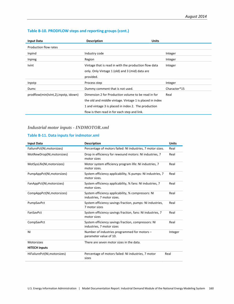
August 2014


Table B-10. PRODFLOW steps and reporting groups (cont.)


Production flow rates



Ivint Vintage that is read in with the production flow data

only. Only Vintage 1 (old) and 3 (mid) data are

provided.

Integer


Dumc Dummy comment that is not used. Character*15

prodflow(min(ivint,2),inpstp, idown) Dimension 2 for Production volume to be read in for

the old and middle vintage. Vintage 1 is placed in index

1 and vintage 3 is placed in index 2. The production

flow is then read in for each step and link.

Real

Industrial motor inputs - INDMOTOR.xml

Table B-11. Data inputs for indmotor.xml

Input Data Description Units FailurePct(NI,motorsizes) Percentage of motors failed: NI industries, 7 motor sizes. Real

MotRewDrop(NI,motorsizes) Drop in efficiency for rewound motors: NI industries, 7 motor sizes

Real

MotSysLife(NI,motorsizes) Motor system efficiency program life: NI industries, 7 motor sizes.

Real

PumpAppPct(NI,motorsizes) System efficiency applicability, % pumps: NI industries, 7 motor sizes.

Real

FanAppPct(NI,motorsizes) System efficiency applicability, % fans: NI industries, 7 motor sizes.

Real

CompAppPct(NI,motorsizes) System efficiency applicability, % compressors: NI industries, 7 motor sizes.

Real

PumpSavPct System efficiency savings fraction, pumps: NI industries, 7 motor sizes

Real

FanSavPct System efficiency savings fraction, fans: NI industries, 7 motor sizes

Real

CompSavPct System efficiency savings fraction, compressors: NI industries, 7 motor sizes

Real

NI Number of industries programmed for motors – parameter value of 10.

Integer

Motorsizes There are seven motor sizes in the data. HITECH inputs

HiFailurePct(NI,motorsizes) Percentage of motors failed: NI industries, 7 motor sizes

Real

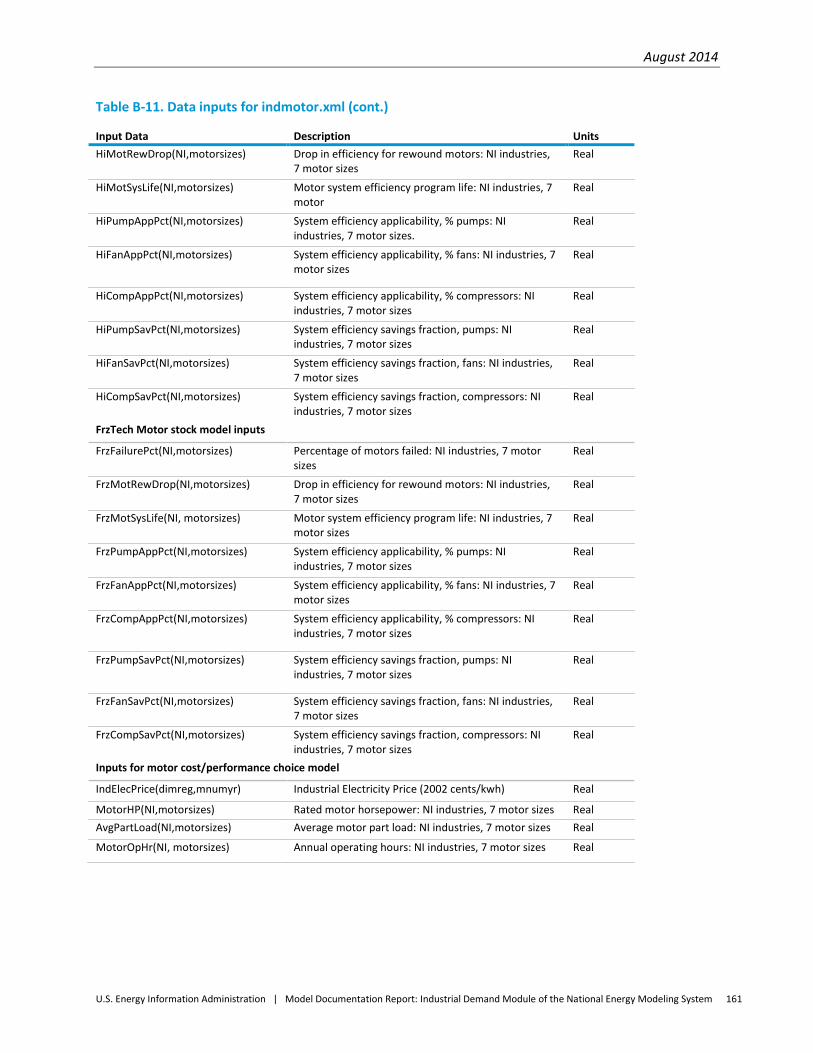
August 2014


Table B-11. Data inputs for indmotor.xml (cont.)

Input Data Description Units HiMotRewDrop(NI,motorsizes) Drop in efficiency for rewound motors: NI industries,

7 motor sizes Real

HiMotSysLife(NI,motorsizes) Motor system efficiency program life: NI industries, 7 motor

Real

HiPumpAppPct(NI,motorsizes) System efficiency applicability, % pumps: NI industries, 7 motor sizes.

Real

HiFanAppPct(NI,motorsizes) System efficiency applicability, % fans: NI industries, 7 motor sizes

Real

HiCompAppPct(NI,motorsizes) System efficiency applicability, % compressors: NI industries, 7 motor sizes

Real

HiPumpSavPct(NI,motorsizes) System efficiency savings fraction, pumps: NI industries, 7 motor sizes

Real

HiFanSavPct(NI,motorsizes) System efficiency savings fraction, fans: NI industries, 7 motor sizes

Real

HiCompSavPct(NI,motorsizes) System efficiency savings fraction, compressors: NI industries, 7 motor sizes

Real

FrzTech Motor stock model inputs

FrzFailurePct(NI,motorsizes) Percentage of motors failed: NI industries, 7 motor sizes

Real

FrzMotRewDrop(NI,motorsizes) Drop in efficiency for rewound motors: NI industries, 7 motor sizes

Real

FrzMotSysLife(NI, motorsizes) Motor system efficiency program life: NI industries, 7 motor sizes

Real

FrzPumpAppPct(NI,motorsizes) System efficiency applicability, % pumps: NI industries, 7 motor sizes

Real

FrzFanAppPct(NI,motorsizes) System efficiency applicability, % fans: NI industries, 7 motor sizes

Real

FrzCompAppPct(NI,motorsizes) System efficiency applicability, % compressors: NI industries, 7 motor sizes

Real

FrzPumpSavPct(NI,motorsizes) System efficiency savings fraction, pumps: NI industries, 7 motor sizes

Real

FrzFanSavPct(NI,motorsizes) System efficiency savings fraction, fans: NI industries, 7 motor sizes

Real

FrzCompSavPct(NI,motorsizes) System efficiency savings fraction, compressors: NI industries, 7 motor sizes

Real

Inputs for motor cost/performance choice model

IndElecPrice(dimreg,mnumyr) Industrial Electricity Price (2002 cents/kwh) Real

MotorHP(NI,motorsizes) Rated motor horsepower: NI industries, 7 motor sizes Real AvgPartLoad(NI,motorsizes) Average motor part load: NI industries, 7 motor sizes Real

MotorOpHr(NI, motorsizes) Annual operating hours: NI industries, 7 motor sizes Real

August 2014


Table B-11. Data inputs for indmotor.xml (cont.)

Input Data Description Units EEPctEff(NI,motorsizes) Efficiency rating for basic motor: NI industries, 7

motor sizes Real

PEPctEff(NI,motorsizes-1) Efficiency rating for "premium" motor: NI industries, 7 motor sizes

Real

RewindCost Cost to rewind failed motors: 7 motor sizes Real

EEListPrice(NI,motorsizes) Purchase price for EPACT minimum (up to 200 hp) or standard efficiency motors: 7 motor sizes

Real

PEListPrice(NI,motorsizes-1) Purchase price for premium efficiency motors (up to 200 hp): 5 motor sizes (2 largest n/a)

Real

DealerDisc(1,motorsizes) Dealer discount on motor purchases, both EPACT and premium efficiency: 7 motor sizes

Real

PremAccept(20) Payback acceptance curve for premium motor purchase

Real

HiTech Inputs for motor cost/performance choice model

HiEEPctEff(NI,motorsizes) Efficiency rating for basic motor: NI industries, 7 motor sizes

Real

HiPEPctEff(NI,motorsizes) Efficiency rating for "premium" motor: NI industries, 7 motor sizes

Real

HiRewindCost(NI,motorsizes) Cost to rewind failed motors: 7 motor sizes Real

HiEEListPrice(NI,motorsizes) Purchase price for EPACT minimum (up to 200 hp) or standard efficiency motors: 7 motor sizes

Real

HiPEListPrice(NI,motorsizes-1) Purchase price for premium efficiency motors (up to 200 hp): 5 motor sizes (2 largest n/a)

Real

HiDealerDisc(1,motorsizes) Dealer discount on motor purchases, both EPACT and premium efficiency: 7 motor sizes

Real

HiPremAccept(20) Payback acceptance curve for premium motor purchase

Real

FrzTech Inputs for motor cost/performance choice model.

FrzEEPctEff(NI,motorsizes) Efficiency rating for basic motor: NI industries, 7 motor sizes

Real

FrzPEPctEff(NI,motorsizes-1) Efficiency rating for "premium" motor: NI industries, 7 motor sizes

Real

FrzRewindCost(NI,motorsizes) Cost to rewind failed motors: 7 motor sizes Real

FrzEEListPrice(NI,motorsizes) Purchase price for EPACT minimum (up to 200 hp) or standard efficiency motors: 7 motor sizes

Real

FrzDealerDisc(1,motorsizes) Dealer discount on motor purchases, both EPACT and premium efficiency: 7 motor sizes

Real

FrzPremAccept(20) Payback acceptance curve for premium motor purchase

Real

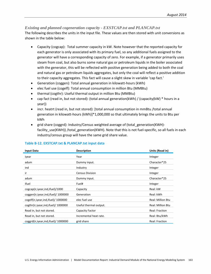
August 2014


Existing and planned cogeneration capacity - EXSTCAP.txt and PLANCAP.txt The following describes the units in the input file. These values are then stored with unit conversions as shown in the table below:

• Capacity (cogcap): Total summer capacity in kW. Note however that the reported capacity for each generator is only associated with its primary fuel, so any additional fuels assigned to the generator will have a corresponding capacity of zero. For example, if a generator primarily uses steam from coal, but also burns some natural gas or petroleum liquids in the boiler associated with the generator, this will be reflected with positive generation being added to both the coal and natural gas or petroleum liquids aggregates, but only the coal will reflect a positive addition to their capacity aggregates. This fact will cause a slight skew in variable ‘cap fact.’

• Generation (coggen): Total annual generation in kilowatt-hours (kWh) • elec fuel use (cogelf): Total annual consumption in million Btu (MMBtu) • thermal (cogthr): Useful thermal output in million Btu (MMBtu) • cap fact (read in, but not stored): (total annual generation(kWh) / (capacity(kW) * hours in a

year)) • incr. heatrt (read in, but not stored): [total annual consumption in mmBtu /total annual

generation in kilowatt-hours (kWh)]*1,000,000 so that ultimately brings the units to Btu per kWh

• grid share (coggrd): Industry/Census weighted average of (total_generation(KWH)-facility_use(KWH)) /total_generation(KWH). Note that this is not fuel-specific, so all fuels in each industry/census group will have the same grid share value.

Table B-12. EXSTCAP.txt & PLANCAP.txt input data

Input Data Description Units (Read in)

iyear Year Integer

adum Dummy input. Character*25

ind Industry Integer

ir Census Division Integer

adum Dummy input. Character*25

ifuel Fuel# Integer

cogcap(ir,iyear,ind,ifuel)/1000 Capacity Real: kW

coggen(ir,iyear,ind,ifuel)/ 1000000 Generation Real: kWh

cogelf(ir,iyear,ind,ifuel)/ 1000000 elec fuel use Real: Million Btu

cogthr(ir,iyear,ind,ifuel)/ 1000000 Useful thermal output. Real: Million Btu

Read in, but not stored. Capacity Factor Real: Fraction

Read in, but not stored. Incremental heat rate. Real: Btu/kWh

coggrd(ir,iyear,ind,ifuel)/ 1000000 grid share Real: Fraction

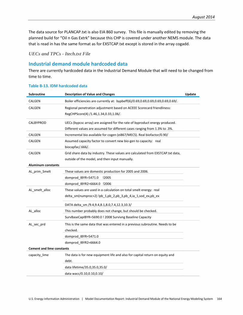
August 2014


The data source for PLANCAP.txt is also EIA 860 survey. This file is manually edited by removing the planned build for “Oil n Gas Extrk” because this CHP is covered under another NEMS module. The data that is read in has the same format as for EXSTCAP.txt except is stored in the array cogadd.

UECs and TPCs - Itech.txt File

Industrial demand module hardcoded data There are currently hardcoded data in the Industrial Demand Module that will need to be changed from time to time.

Table B-13. IDM hardcoded data

Subroutine Description of Value and Changes Update

CALGEN Boiler efficiencies are currently at: bypbeff(6)/0.69,0.69,0.69,0.69,0.69,0.69/.

CALGEN Regional penetration adjustment based on ACEEE Scorecard friendliness:

RegCHPScore(4) /1.46,1.34,0.33,1.06/.

CALBYPROD UECs (bypcsc array) are assigned for the rate of byproduct energy produced.

Different values are assumed for different cases ranging from 1.3% to .3%.

CALGEN Incremental bio available for cogen (ei867/MECS). Real biofactor/0.90/

CALGEN Assumed capacity factor to convert new bio-gen to capacity: real

biocapfac/.666/.

CALGEN Grid share data by industry. These values are calculated from EXSTCAP.txt data,

outside of the model, and then input manually.

Aluminum constants

AL_prim_Smelt These values are domestic production for 2005 and 2006.

domprod_IBYR=5471.0 !2005

domprod_IBYR2=6664.0 !2006

AL_smelt_alloc These values are used in a calculation on total smelt energy: real

delta_sm(numproc+2) !pb_1,pb_2,pb_3,pb_4,ia_1,sod_ex,pb_ex

DATA delta_sm /9.4,9.4,8.1,8.0,7.4,12.3,10.3/

AL_alloc This number probably does not change, but should be checked.

SurvBaseCapIBYR=5690.0 ! 2008 Survivng Baseline Capacity

AL_sec_prd This is the same data that was entered in a previous subroutine. Needs to be

checked.

domprod_IBYR=5471.0

domprod_IBYR2=6664.0

Cement and lime constants

capacity_lime The data is for new equipment life and also for capital return on equity and

debt.

data lifetime/35.0,35.0,35.0/

data wacc/0.10,0.10,0.10/

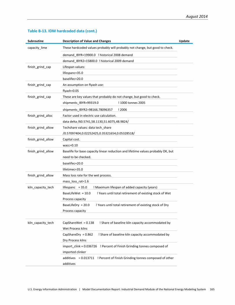
August 2014


Table B-13. IDM hardcoded data (cont.)


capacity_lime These hardcoded values probably will probably not change, but good to check.

demand_IBYR=19900.0 ! historical 2008 demand

demand_IBYR2=15800.0 ! historical 2009 demand

finish_grind_cap Lifespan values:

lifespanc=35.0

baselifec=20.0

finish_grind_cap An assumption on flyash use:

flyash=0.05

finish_grind_cap These are key values that probably do not change, but good to check.

shipments_IBYR=99319.0 ! 1000 tonnes 2005

shipments_IBYR2=98166.78096357 ! 2006

finish_grind_alloc Factor used in electric use calculation.

data delta /60.5741,58.1130,51.6075,48.9824/

finish_grind_allow Techshare values: data tech_share

/0.57097404,0.02252425,0.35321654,0.05328518/

finish_grind_allow Capital cost.

wacc=0.10

finish_grind_allow Baselife for base capacity linear reduction and lifetime values probably OK, but

need to be checked.

baselifec=20.0

lifetimec=35.0

finish_grind_allow Mass loss rate for the wet process.

mass_loss_rat=1.6

kiln_capacity_tech lifespanc = 35.0 ! Maximum lifespan of added capacity (years)

BaseLifeWet = 10.0 ! Years until total retirement of existing stock of Wet

Process capacity

BaseLifeDry = 20.0 ! Years until total retirement of existing stock of Dry

Process capacity

kiln_capacity_tech CapShareWet = 0.138 ! Share of baseline kiln capacity accommodated by

Wet Process kilns

CapShareDry = 0.862 ! Share of baseline kiln capacity accommodated by

Dry Process kilns

import_clink = 0.036726 ! Percent of Finish Grinding tonnes composed of

imported clinker

additives = 0.013711 ! Percent of Finish Grinding tonnes composed of other

additives

August 2014




kiln_capacity calibrationc=11.0

lifespanc=35.0

baselifec=20.0

import_clink=0.036726

additives=0.013711

kiln_allocation data tech_share/0.719609,0.140195,0.140195/

data heat_coeff/5.86,2.8714,3.13369,2.93/

data elec_coeff/-93.6517,183.2891,189.4978,187.0295/

data delta /105.55612,106.83334,106.09772/

kiln_allocation baselifec=20.0

lifetimec=35.0

wacc=0.10

kiln_allocation Wet and dry process shares for baseline capacity.

pwet=0.138

pdry=0.862

burner_capacity Probably OK, but good to check.

lifespanc=25.0

baselifec=20.0

burner_allocation wet_coeff/0.0022157,0.044315,0.008562,0.017124,0.5486,0.3792/ !

CIMS Data, Allocation by Burner Type (Wet Process)

data

burner_coeff/1.2611237,1.1663024,1.2137131,1.1947488,1.1947488,1.19474/

data heatd_coeff/5.86/

data

tech_share/0.0057773,0.0212896,0.0050006,0.0171243,0.7310437,0.2197645/

data calib_coeff/500.0,100000.0,2000000.0,0.0 /!fixed cost,fuel

cost,emissions,particulate emissions

burner_allocation alpha_burner(1)=-4.5852

alpha_burner(2)=-3.3306



alpha_burner(5)=0.0


August 2014




burner_allocation lifetimec=25.0

wacc=0.10

baselifec=20.0

raw_grind_capacity Values probably OK.

lifespanc=35.0

baselifeg=20.0

raw_grind_capacity Seems like a value that could change from year to year.

massloss=1.6

raw_grind_alloc data tech_split/0.489,0.511/

data wet_coeff/161.0,156.0/ ! CIMS Data, Allocation by Mill Type (Wet

Process)

data tech_share/0.43,0.57/

data calib_coeff/1.0,500.0,500.0,1000000.0/

data delta /75.29,72.44/

alpha_rg(1)=0.0

alpha_rg(2)=-0.45985411

raw_grind_alloc wacc=0.10

baselifec=20.0

lifetimec=35.0

August 2014


Appendix C. Descriptions of Major Industrial Groups and Selected Industries This appendix contains descriptions of industrial groups and selected industries taken from the North American Industry Classification System (NAICS). This appendix includes general descriptions of the 15 manufacturing and 6 non-manufacturing groups that comprise the industries modeled in the Industrial Demand Module. NAICS is the standard used by federal statistical agencies in classifying business establishments for the purpose of collecting, analyzing, and publishing statistical data related to the U.S. business economy.

NAICS 11 - The Agriculture, Forestry, Fishing and Hunting sector comprises establishments primarily engaged in growing crops, raising animals, harvesting timber, and harvesting fish and other animals from a farm, ranch, or their natural habitats.

The establishments in this sector are often described as farms, ranches, dairies, greenhouses, nurseries, orchards, or hatcheries. A farm may consist of a single tract of land or a number of separate tracts which may be held under different tenures. For example, one tract may be owned by the farm operator and another rented. It may be operated by the operator alone or with the assistance of members of the household or hired employees, or it may be operated by a partnership, corporation, or other type of organization. When a landowner has one or more tenants, renters, croppers, or managers, the land operated by each is considered a farm.

The sector distinguishes two basic activities: agricultural production and agricultural support activities. Agricultural production includes establishments performing the complete farm or ranch operation, such as farm owner-operators, tenant farm operators, and sharecroppers. Agricultural support activities include establishments that perform one or more activities associated with farm operation, such as soil preparation, planting, harvesting, and management, on a contract or fee basis.

NAICS 21 - The Mining, Quarrying, and Oil and Gas Extraction sector comprises establishments that extract naturally occurring mineral solids, such as coal and ores; liquid minerals, such as crude petroleum; and gases, such as natural gas. The term mining is used in the broad sense to include quarrying, well operations, beneficiating (e.g., crushing, screening, washing, and flotation), and other preparation customarily performed at the mine site, or as a part of mining activity.

The Mining, Quarrying, and Oil and Gas Extraction sector distinguishes two basic activities: mine operation and mining support activities. Mine operation includes establishments operating mines, quarries, or oil and gas wells on their own account or for others on a contract or fee basis. Mining support activities include establishments that perform exploration (except geophysical surveying) and/or other mining services on a contract or fee basis (except mine site preparation and construction of oil/gas pipelines).

Establishments in the Mining, Quarrying, and Oil and Gas Extraction sector are grouped and classified according to the natural resource mined or to be mined. Industries include establishments that develop

August 2014


the mine site, extract the natural resources, and/or those that beneficiate (i.e., prepare) the mineral mined. Beneficiation is the process whereby the extracted material is reduced to particles that can be separated into mineral and waste, the former suitable for further processing or direct use. The operations that take place in beneficiation are primarily mechanical, such as grinding, washing, magnetic separation, and centrifugal separation. In contrast, manufacturing operations primarily use chemical and electrochemical processes, such as electrolysis and distillation. However, some treatments, such as heat treatments, take place in both the beneficiation and the manufacturing (i.e., smelting/refining) stages. The range of preparation activities varies by mineral and the purity of any given ore deposit. While some minerals, such as petroleum and natural gas, require little or no preparation, others are washed and screened, while yet others, such as gold and silver, can be transformed into bullion before leaving the mine site.

NAICS 23 - The Construction sector comprises establishments primarily engaged in the construction of buildings or engineering projects (e.g., highways and utility systems). Establishments primarily engaged in the preparation of sites for new construction and establishments primarily engaged in subdividing land for sale as building sites also are included in this sector.

Construction work done may include new work, additions, alterations, or maintenance and repairs. Activities of these establishments generally are managed at a fixed place of business, but they usually perform construction activities at multiple project sites. Production responsibilities for establishments in this sector are usually specified in (1) contracts with the owners of construction projects (prime contracts) or (2) contracts with other construction establishments (subcontracts).

NAICS 311 - Industries in the Food Manufacturing subsector transform livestock and agricultural products into products for intermediate or final consumption. The industry groups are distinguished by the raw materials (generally of animal or vegetable origin) processed into food products.

The food products manufactured in these establishments are typically sold to wholesalers or retailers for distribution to consumers, but establishments primarily engaged in retailing bakery and candy products made on the premises not for immediate consumption are included.

NAICS 312 - Industries in the Beverage and Tobacco Product Manufacturing subsector manufacture beverages and tobacco products. The industry group, Beverage Manufacturing, includes three types of establishments: (1) those that manufacture nonalcoholic beverages; (2) those that manufacture alcoholic beverages through the fermentation process; and (3) those that produce distilled alcoholic beverages. Ice manufacturing, while not a beverage, is included with nonalcoholic beverage manufacturing because it uses the same production process as water purification.

In the case of activities related to the manufacture of beverages, the structure follows the defined production processes. Brandy, a distilled beverage, was not placed under distillery product manufacturing, but rather under the NAICS class for winery product manufacturing since the production process used in the manufacturing of alcoholic grape-based beverages produces both wines (fermented beverage) and brandies (distilled beverage).

August 2014


The industry group, Tobacco Manufacturing, includes two types of establishments: (1) those engaged in redrying and stemming tobacco and, (2) those that manufacture tobacco products, such as cigarettes and cigars.

NAICS 313 - Industries in the Textile Mills subsector group establishments that transform a basic fiber (natural or synthetic) into a product, such as yarn or fabric that is further manufactured into usable items, such as apparel, sheets, towels, and textile bags for individual or industrial consumption. The further manufacturing may be performed in the same establishment and classified in this subsector, or it may be performed at a separate establishment and be classified elsewhere in manufacturing.

NAICS 314 - Industries in the Textile Product Mills subsector group establishments that make textile products (except apparel). With a few exceptions, processes used in these industries are generally cut and sew (i.e., purchasing fabric and cutting and sewing to make nonapparel textile products, such as sheets and towels).

NAICS 315 - Industries in the Apparel Manufacturing subsector group establishments with two distinct manufacturing processes: (1) cut and sew (i.e., purchasing fabric and cutting and sewing to make a garment), and (2) the manufacture of garments in establishments that first knit fabric and then cut and sew the fabric into a garment.

NAICS 316 - Establishments in the Leather and Allied Product Manufacturing subsector transform hides into leather by tanning or curing and fabricating the leather into products for final consumption. It also includes the manufacture of similar products from other materials, including products (except apparel) made from "leather substitutes," such as rubber, plastics, or textiles. Rubber footwear, textile luggage, and plastic purses or wallets are examples of "leather substitute" products included in this group.

NAICS 321 - Industries in the Wood Product Manufacturing subsector manufacture wood products, such as lumber, plywood, veneers, wood containers, wood flooring, wood trusses, manufactured homes (i.e., mobile homes), and prefabricated wood buildings. The production processes of the Wood Product Manufacturing subsector include sawing, planing, shaping, laminating, and assembling of wood products starting from logs that are cut into bolts, or lumber that then may be further cut, or shaped by lathes or other shaping tools. The lumber or other transformed wood shapes may also be subsequently planed or smoothed, and assembled into finished products, such as wood containers. The Wood Product Manufacturing subsector includes establishments that make wood products from logs and bolts that are sawed and shaped, and establishments that purchase sawed lumber and make wood products. With the exception of sawmills and wood preservation establishments, the establishments are grouped into industries mainly based on the specific products manufactured.

NAICS 322 - Industries in the Paper Manufacturing subsector make pulp, paper, or converted paper products. The manufacturing of these products is grouped together because they constitute a series of vertically connected processes. More than one is often carried out in a single establishment. There are essentially three activities. The manufacturing of pulp involves separating the cellulose fibers from other impurities in wood or used paper. The manufacturing of paper involves matting these fibers into a sheet. Converted paper products are made from paper and other materials by various cutting and shaping techniques and include coating and laminating activities.

August 2014


The Paper Manufacturing subsector is subdivided into two industry groups, the first for the manufacturing of pulp and paper and the second for the manufacturing of converted paper products. Paper making is treated as the core activity of the subsector. Therefore, any establishment that makes paper (including paperboard), either alone or in combination with pulp manufacturing or paper converting, is classified as a paper or paperboard mill. Establishments that make pulp without making paper are classified as pulp mills. Pulp mills, paper mills and paperboard mills comprise the first industry group.

Establishments that make products from purchased paper and other materials make up the second industry group, Converted Paper Product Manufacturing. This general activity is then subdivided based, for the most part, on process distinctions. Paperboard container manufacturing uses corrugating, cutting, and shaping machinery to form paperboard into containers. Paper bag and coated and treated paper manufacturing establishments cut and coat paper and foil. Stationery product manufacturing establishments make a variety of paper products used for writing, filing, and similar applications. 0ther converted paper product manufacturing includes, in particular, the conversion of sanitary paper stock into such things as tissue paper and disposable diapers.

NAICS 323 - Industries in the Printing and Related Support Activities subsector print products, such as newspapers, books, labels, business cards, stationery, business forms, and other materials, and perform support activities, such as data imaging, platemaking services, and bookbinding. The support activities included here are an integral part of the printing industry, and a product (a printing plate, a bound book, or a computer disk or file) that is an integral part of the printing industry is almost always provided by these operations.

Processes used in printing include a variety of methods used to transfer an image from a plate, screen, film, or computer file to some medium, such as paper, plastics, metal, textile articles, or wood. The most prominent of these methods is to transfer the image from a plate or screen to the medium (lithographic, gravure, screen, and flexographic printing). A rapidly growing new technology uses a computer file to directly "drive" the printing mechanism to create the image and new electrostatic and other types of equipment (digital or nonimpact printing).

NAICS 324 - The Petroleum and Coal Products Manufacturing subsector is based on the transformation of crude petroleum and coal into usable products. The dominant process is petroleum refining that involves the separation of crude petroleum into component products through such techniques as cracking and distillation.

NAICS 325 - The Chemical Manufacturing subsector is based on the transformation of organic and inorganic raw materials by a chemical process and the formulation of products. This subsector distinguishes the production of basic chemicals that comprise the first industry group from the production of intermediate and end products produced by further processing of basic chemicals that make up the remaining industry groups.

NAICS 326 - Industries in the Plastics and Rubber Products Manufacturing subsector make goods by processing plastics materials and raw rubber. The core technology employed by establishments in this subsector is that of plastics or rubber product production. Plastics and rubber are combined in the same

August 2014


subsector because plastics are increasingly being used as a substitute for rubber; however the subsector is generally restricted to the production of products made of just one material, either solely plastics or rubber.

Many manufacturing activities use plastics or rubber, for example the manufacture of footwear or furniture. Typically, the production process of these products involves more than one material. In these cases, technologies that allow disparate materials to be formed and combined are of central importance in describing the manufacturing activity. In NAICS, such activities (the footwear and furniture manufacturing) are not classified in the Plastics and Rubber Products Manufacturing subsector because the core technologies for these activities are diverse and involve multiple materials.

NAICS 327 - The Nonmetallic Mineral Product Manufacturing subsector transforms mined or quarried nonmetallic minerals, such as sand, gravel, stone, clay, and refractory materials, into products for intermediate or final consumption. Processes used include grinding, mixing, cutting, shaping, and honing. Heat often is used in the process and chemicals are frequently mixed to change the composition, purity, and chemical properties for the intended product.

The Nonmetallic Mineral Product Manufacturing subsector includes establishments that manufacture products, such as bricks, refractories, ceramic products, and glass and glass products, such as plate glass and containers. Also included are cement and concrete products, lime, gypsum and other nonmetallic mineral products including abrasive products, ceramic plumbing fixtures, statuary, cut stone products, and mineral wool. The products are used in a wide range of activities from construction and heavy and light manufacturing to articles for personal use.

The IDM models the following three industries in NAICS 327.

NAICS 327310 - Cement Manufacturing

The Cement Manufacturing industry comprises establishments primarily engaged in manufacturing portland, natural, masonry, pozzolanic, and other hydraulic cements. Cement manufacturing establishments may calcine earths or mine, quarry, manufacture, or purchase lime.

NAICS 327410 - Lime Manufacturing

The Lime Manufacturing industry comprises establishments primarily engaged in manufacturing lime from calcitic limestone, dolomitic limestone, or other calcareous materials, such as coral, chalk, and shells. Lime manufacturing establishments may mine, quarry, collect, or purchase the sources of calcium carbonate.

NAICS 3272—Glass manufacturing

The Glass Manufacturing industry produces glass is produced by heating silica sand to the melting point sometimes combined with cullet, or recycled glass. Establishments in this industry produce flat glass, blown glass, and container glass. The IDM also includes mineral wool, or fiber glass in the glass model. Mineral wool is NAICS 32799.

August 2014


NAICS 331 - Industries in the Primary Metal Manufacturing subsector smelt and/or refine ferrous and nonferrous metals from ore, pig or scrap, using electrometallurgical and other process metallurgical techniques. Establishments in this subsector also manufacture metal alloys and superalloys by introducing other chemical elements to pure metals. The output of smelting and refining, usually in ingot form, is used in rolling, drawing, and extruding operations to make sheet, strip, bar, rod, or wire, and in molten form to make castings and other basic metal products.

Primary manufacturing of ferrous and nonferrous metals begins with ore or concentrate as the primary input. Establishments manufacturing primary metals from ore and/or concentrate remain classified in the primary smelting, primary refining, or iron and steel mill industries regardless of the form of their output. Establishments primarily engaged in secondary smelting and/or secondary refining recover ferrous and nonferrous metals from scrap and/or dross. The output of the secondary smelting and/or secondary refining industries is limited to shapes, such as ingot or billet, that will be further processed. Recovery of metals from scrap often occurs in establishments that are primarily engaged in activities such as rolling, drawing, extruding, or similar processes.

NAICS 332 - Industries in the Fabricated Metal Product Manufacturing subsector transform metal into intermediate or end products, other than machinery, computers and electronics, and metal furniture, or treat metals and metal formed products fabricated elsewhere. Important fabricated metal processes are forging, stamping, bending, forming, and machining, used to shape individual pieces of metal; and other processes, such as welding and assembling, used to join separate parts together. Establishments in this subsector may use one or a combination of these processes.

NAICS 333 - Industries in the Machinery Manufacturing subsector create end products that apply mechanical force, for example, the application of gears and levers, to perform work. Some important processes for the manufacture of machinery are forging, stamping, bending, forming, and machining that are used to shape individual pieces of metal. Processes, such as welding and assembling are used to join separate parts together. Although these processes are similar to those used in metal fabricating establishments, machinery manufacturing is different because it typically employs multiple metal-forming processes in manufacturing the various parts of the machine. Moreover, complex assembly operations are an inherent part of the production process.

NAICS 334 - Industries in the Computer and Electronic Product Manufacturing subsector group establishments that manufacture computers, computer peripherals, communications equipment, and similar electronic products, and establishments that manufacture components for such products. The Computer and Electronic Product Manufacturing industries have been combined in the hierarchy of NAICS because of the economic significance they have attained. Their rapid growth suggests that they will become even more important to the economies of all three North American countries in the future, and in addition their manufacturing processes are fundamentally different from the manufacturing processes of other machinery and equipment. The design and use of integrated circuits and the application of highly specialized miniaturization technologies are common elements in the production technologies of the computer and electronic subsector. Convergence of technology motivates this NAICS subsector. Digitalization of sound recording, for example, causes both the medium (the compact disc) and the equipment to resemble the technologies for recording, storing, transmitting, and manipulating

August 2014


data. Communications technology and equipment have been converging with computer technology. When technologically-related components are in the same sector, it makes it easier to adjust the classification for future changes, without needing to redefine its basic structure. The creation of the Computer and Electronic Product Manufacturing subsector assists in delineating new and emerging industries because the activities that will serve as the probable sources of new industries, such as computer manufacturing and communications equipment manufacturing, or computers and audio equipment, are brought together. As new activities emerge, therefore, they are less likely to cross the subsector boundaries of the classification.

NAICS 335 - Industries in the Electrical Equipment, Appliance, and Component Manufacturing subsector manufacture products that generate, distribute and use electrical power. Electric Lighting Equipment Manufacturing establishments produce electric lamp bulbs, lighting fixtures, and parts. Household Appliance Manufacturing establishments make both small and major electrical appliances and parts. Electrical Equipment Manufacturing establishments make goods, such as electric motors, generators, transformers, and switchgear apparatus. Other Electrical Equipment and Component Manufacturing establishments make devices for storing electrical power (e.g., batteries), for transmitting electricity (e.g., insulated wire), and wiring devices (e.g., electrical outlets, fuse boxes, and light switches).

NAICS 336 - Industries in the Transportation Equipment Manufacturing subsector produce equipment for transporting people and goods. Transportation equipment is a type of machinery. An entire subsector is devoted to this activity because of the significance of its economic size in all three North American countries.

Establishments in this subsector use production processes similar to those of other machinery manufacturing establishments—bending, forming, welding, machining, and assembling metal or plastic parts into components and finished products. However, the assembly of components and subassemblies and their further assembly into finished vehicles tends to be a more common production process in this subsector than in the Machinery Manufacturing subsector.

NAICS 337 - Industries in the Furniture and Related Product Manufacturing subsector make furniture and related articles, such as mattresses, window blinds, cabinets, and fixtures. The processes used in the manufacture of furniture include the cutting, bending, molding, laminating, and assembly of such materials as wood, metal, glass, plastics, and rattan. However, the production process for furniture is not solely bending metal, cutting and shaping wood, or extruding and molding plastics. Design and fashion trends play an important part in the production of furniture. The integrated design of the article for both esthetic and functional qualities is also a major part of the process of manufacturing furniture. Design services may be performed by the furniture establishments’ work force or may be purchased from industrial designers.

NAICS 339 - Industries in the Miscellaneous Manufacturing subsector make a wide range of products that cannot readily be classified in specific NAICS subsectors in manufacturing. Processes used by these establishments vary significantly, both among and within industries. For example, a variety of manufacturing processes are used in manufacturing sporting and athletic goods that include products

August 2014


such as tennis racquets and golf balls. The processes for these products differ from each other, and the processes differ significantly from the fabrication processes used in making dolls or toys, the melting and shaping of precious metals to make jewelry, and the bending, forming, and assembly used in making medical products.

August 2014


Appendix D. Bibliography American Council for an Energy-Efficient Economy, Energy-Efficient Motor Systems: A Handbook on Technology, Program, and Policy Opportunities, Second Edition, Washington, DC, 2002.

American Council for an Energy-Efficient Economy, “Challenges Facing Combined Heat and Power Today: A State-by-State Assessment,” Washington, DC, September 2011, http://aceee.org/research-report/ie111 .

Centre for the Analysis and Dissemination of Demonstrated Energy Technologies, Learning from experiences with Gas-Turbine-Based CHP in Industry, CADDET IEA/OECD, The Netherlands, April 1993.

Centre for the Analysis and Dissemination of Demonstrated Energy Technologies, Learning from experiences with Small-Scale Cogeneration, CADDET IEA/OECD, The Netherlands, November 1995.

Dahl, Carol, A Survey of Energy Demand Elasticities in Support of the Development of the NEMS, prepared for the U.S. Energy Information Administration, Washington, DC, October 1993.

Energy and Environmental Analysis, Inc., Characterization of the U.S. Industrial Commercial Boiler Population, submitted to Oak Ridge National Laboratory, Arlington, VA, May 2005.

Energy and Environmental Analysis, Inc., NEM Industrial Prototype Model Documentation (Draft), submitted to Energy Information Administration, Arlington, VA, August 2008.

Executive Office of the President, Office of Management and Budget, North American Industry Classification System, United States. Washington, DC, 2007.

FOCIS Associates, Inc., Industrial Technology and Data Analysis Supporting the NEMS Industrial Model, unpublished report prepared for the Office of Integrated Analysis and Forecasting, Energy Information Administration, Washington, DC, October 2005.

Johnson Controls Inc., 2009 Energy Efficiency Indicator IFMA Summary Report, International Facility Management Association, www.ifma.org, 2009.

NESCAUM, Applicability and Feasibility of NOX, SO2, and PM Emissions Control Technologies for Industrial, Commercial, and Institutional (ICI) Boilers, January 2009.

Portland Cement Association, “U.S. Detail Cement Plant Information.”

Roop, Joseph M. and Chris Bataille, “Modeling Climate Change Policies in the US and Canada: A Progress Report,” p. 7. Presentation to 26th USAEE/IAEE North American Conference, September 27, 2006,

SRA International, “Report on the Analysis and Modeling Approach to Characterize and Estimate Fuel Use by End-Use Applications in the Agriculture and Construction Industries,” unpublished report prepared for the U.S Energy Information Administration, March 2011.

SAIC, “Model Documentation Report the U.S. Cement Industry,” unpublished data report prepared for the Office of Energy Analysis, U.S. Energy Information Administration, Washington, DC, August 2012.



http://www.ifma.org/

August 2014


SAIC, “Model Documentation Report the U.S. Lime Industry,” unpublished data report prepared for the Office of Energy Analysis, U.S. Energy Information Administration, Washington, DC, August 2012.

SAIC, “Model Documentation Report the U.S. Aluminum Industry,” unpublished data report prepared for the Office of Energy Analysis, U.S. Energy Information Administration, Washington, DC, June 2013.

SENTECH Inc., Commercial and Industrial CHP Technology Cost and Performance Data for EIA, report prepared for the Office of Integrated Analysis and Forecasting, Energy Information Administration, Washington, DC, June 2010.

U.S. Department of Agriculture, National Agricultural Statistical Service, 2007 Census of Agriculture, Washington, DC, February 2009.

U.S. Department of Agriculture, Economic Research Service, Commodity Costs and Returns, Energy Use on Major Field Crops in Surveyed States 2001, Washington, DC, 2002.

U.S. Department of Commerce, Census Bureau, Annual Survey of Manufactures, Fuels and Electric Energy Consumed, Washington, DC, Various Years.

U.S. Department of Commerce, Census Bureau, Economic Census 2007: Construction Industry Series; Manufacturing Industry Series; Mining Industry Series, available at http://www.census.gov/econ/census07/.

U.S. Department of Energy, MotorMaster+ 4.0 software database, 2007, available at http://www1.eere.energy.gov/industry/bestpractices/pdfs/mmplus.pdf..

U.S. Department of Energy, United States Industrial Electric Motor Systems Market Opportunities Assessment, Burlington, MA, December 1998.

U.S. Department of the Interior, United States Geological Survey, Minerals Yearbook 2006 available at http://minerals.usgs.gov/minerals/pubs/commodity/cement/myb1-2006-cemen.pdf.

U.S. Department of the Interior, United States Geological Survey, Minerals Yearbook 2010 (Advance Release) available at http://minerals.usgs.gov/minerals/pubs/commodity/cement/myb1-2010-cemen.pdf

U.S. Department of the Interior, United States Geological Survey, Minerals Yearbook 2011 available at http://minerals.usgs.gov/minerals/pubs/commodity/aluminum/myb1-2011-alumi.pdf.

U.S. Energy Information Administration, Annual Energy Outlook 2014. DOE/EIA-0383(2013), Washington, DC, May 2013.

U.S. Energy Information Administration, Annual Energy Review 2013, DOE/EIA-0384 (2012), Washington, DC, June 2012.

http://www.census.gov/econ/census07/

http://www1.eere.energy.gov/industry/bestpractices/pdfs/mmplus.pdf

http://minerals.usgs.gov/minerals/pubs/commodity/cement/myb1-2006-cemen.pdf



http://minerals.usgs.gov/minerals/pubs/commodity/aluminum/myb1-2011-alumi.pdf

August 2014


U.S. Energy Information Administration, Assumptions Report to the Annual Energy Outlook 2014., (Washington, DC), June 2014. Industrial section link: http://www.eia.gov/forecasts/aeo/assumptions/pdf/industrial.pdf.

U.S. Energy Information Administration, Documentation of the Commercial Sector Demand Module (CDM), DOE/EIA-M066(2011), Washington, DC, July 2011.

U.S. Energy Information Administration, Documentation of the Oil and Gas Supply Module (OGSM), DOE/EIA-M063(2011), Washington, DC, July 2011.

U.S. Energy Information Administration, Documentation of the Transportation Sector Module (TDM), DOE/EIA-M071(2011), Washington, DC, July 2011.

U.S. Energy Information Administration, Documentation of Liquid Fuels Market Module, DOE/EIA-M059(2013), Washington, DC, December 2013.

U.S. Energy Information Administration (EIA), 2010 Manufacturing Energy Consumption Survey, http://www.eia.gov/consumption/manufacturing/, Washington, DC, March 2013.

U.S. Energy Information Administration, Short-Term Energy Outlook (Washington, DC) September 2013, http://www.eia.gov/forecasts/steo/archives/sep13.pdf.

U.S. Energy Information Administration, State Energy Data Report, Consumption Estimates 1960-2011, (Washington, DC) June 2013, http://www.eia.gov/state/seds/.

U.S. Geological Service, Mineral Commodity Summaries, (Washington, DC) 2012, http://minerals.usgs.gov/minerals/pubs/commodity/aluminum/mcs-2012-alumi.pdf

http://www.eia.gov/forecasts/aeo/assumptions/pdf/industrial.pdf

http://www.eia.gov/consumption/manufacturing/

http://www.eia.gov/forecasts/steo/archives/sep13.pdf


http://minerals.usgs.gov/minerals/pubs/commodity/aluminum/mcs-2012-alumi.pdf

Documents

Model Documentation Report: Industrial Demand Module of the National Energy Modeling ...2014).pdf · 2014-08-06 · August 2014 U.S. Energy Information Administration | Model Documentation