Model-Based Validation of QoS Properties of BiomedicalSensor Networks �

[Extended Abstract]

Simon TschirnerUppsala University

P.O. Box 337751 05 Uppsala, Sweden

simon.tschirner@it.uu.se

Liang XuedongRikshospitalet University

Hospital and University of OsloP.O. Box 1139

N-0316 Oslo, Norwayxuedongl@medisin.uio.no

Wang YiUppsala University

P.O. Box 337751 05 Uppsala, Sweden

yi@it.uu.se

ABSTRACTA Biomedical Sensor Network (BSN) is a small-size sensornetwork for medical applications, that may contain tens ofsensor nodes. In this paper, we present a formal modelfor BSNs using timed automata, where the sensor nodescommunicate using the Chipcon CC2420 transceiver (devel-oped by Texas Instruments) according to the IEEE 802.15.4standard. Based on the model, we have used UPPAAL tovalidate and tune the temporal configuration parameters ofa BSN in order to meet desired QoS requirements on net-work connectivity, packet delivery ratio and end-to-end de-lay. The network studied allows dynamic reconfigurationsof the network topology due to the temporally switchingof sensor nodes to power-down mode for energy-saving ortheir physical movements. Both the simulator and model-checker of UPPAAL are used to analyze the average-caseand worst-case behaviours. To enhance the scalability ofthe tool, we have implemented a (new text-based) versionof the UPPAAL simulator optimized for exploring symbolictraces of automata containing large data structures such asmatrices. Our experiments show that even though the mainfeature of the tool is model checking, it is also a promisingand competitive tool for efficient simulation and parame-ter tuning. The simulator scales well; it can easily handleup to 50 nodes in our experiments. The model checker in-stalled on a notebook can also deal with networks with 5up to 16 nodes within minutes depending on the proper-ties checked; these are BSNs of reasonable size for medicalapplications. Finally, to study the accuracy of our modeland analysis results, we compare simulation results by UP-PAAL for two medical scenarios with traditional simulationtechniques. The comparison shows that our analysis resultscoincide closely with simulation results by OMNeT++, awidely used simulation tool for wireless sensor networks.

�The work is supported by EC IST project CREDO.

All models for the experiments of this work can be found athttp://www.it.uu.se/research/group/darts/bsn/ including XML files for theUPPAAL models of Chipcon CC2240 transceiver and BSNs analyzed, andaslo source files for OMNeT++ simulation.

1. INTRODUCTIONWireless Sensor Networks (WSN) [2] contain hundreds orthousands of sensor nodes equipped with sensing, computingand communication devices. These sensor nodes may be dis-tributed in a large area and connected by short-range com-munication devices over wireless channels. WSNs have a lotof potential applications, e.g., battlefield surveillance, wild-life monitoring and medical applications. In these mission-critical applications, a certain set of QoS requirements onnetwork performance must be satisfied. This poses a num-ber of challenges on the design and analysis of WSNs. Due tothe severe constraints on hardware platform, dynamic work-ing environments, and self-organizing manner, a key designchallenge is to evaluate the network performance without in-vesting on the hardware platforms and the time-consumingdeployment and measurement.

In this paper, we demonstrate that model-based techniquescan be used as an alternative approach to the design andanalysis of WSNs to complement traditional simulation-basedtechniques. We shall study Biomedical Sensor Networks(BSN), which are small-size WSNs for medical applications.A BSN may contain tens of sensor nodes with a specifiedsink node, distributed over a limited area such as an opera-tion room or a nursing home. However, due to the hardwareconstraints and limited power supply, the range of wirelesscommunication for each individual node is highly bounded.Thus a packet often has to be forwarded by a number ofnodes to reach its destination. A concrete application sce-nario of BSNs is described in [15]. On an accident site diffi-cult to access, there may be many injured persons and theavailable medics are limited. In such a situation a quicklydeployed BSN on the accident victims may be used to collectand transmit vital sign data to a centralized medical serverfor diagnose and analysis so that proper and efficient medicaloperations can be carried out. For example, a sensor nodemay be used to measure the body temperature of an injuredperson with a certain period, and send the measured datato the sink node immediately or when it reaches a thresh-old value. Due to the life-critical nature of the application,certain QoS requirements on, e.g., network connectivity andpacket delivery ratio must be guaranteed.

The difficulty in designing and analyzing a BSN is not indealing with an individual sensor node in the network, which

may be running a simple software. But as the network con-tains a number of nodes, and these nodes must cooperateto achieve some common goal, the behaviour of such a net-work is extremely more complicated and difficult to analyzedue to non-determinism. For instance, the network topol-ogy may be changing dynamically. The sensor nodes maymove, disappear, and new nodes may appear from time totime. To achieve the common goal, the sensor nodes in anetwork need to follow a suitable communication protocol.The IEEE 802.15.4 [1] standard for wireless communicationis one of such protocols. It offers different modes for com-munication and algorithms for packet routing if no directconnection to the sink exists. However, the specificationof the standard covers only the logical behaviour of a sen-sor node in wireless communication. Temporal configura-tion parameters, such as the active and standby period, of anode must be determined according to the application andthe QoS requirements to be satisfied. For example, the ap-plication defines how often a sensor node should transmitmeasured data and the necessary bandwidth. The durationa node spends in the power down mode or in a mode forpacket forwarding can also be carefully set to reduce energyconsumption.

(a)

PowerDown

TXRX

AckTX

(b)

Figure 1: Timing parameters and operation statesof Chipcon CC2420 based sensor nodes.

Fig. 1(a) illustrates the main timing parameters associatedwith a sensor node. It has a main period covering three mainmodes: transmission, reception and power down (sleeping).The behaviour of a node repeats over the main periods. Itmay, for instance, represent the measurement frequency ofthe sensor. The second main parameter is the active period.Within a main period, a node may stay active for some timeand then switch to the power down mode. When it becomesactive again, the node may begin to transmit data imme-diately or after a short delay. Within the active period, ifa node is not transmitting data, it can receive data. Thereceived data may need to be forwarded, which brings thenode to the transmission mode again. The technical chal-lenge here is to tune and validate the timing parameters suchthat the desired QoS requirements are satisfied. In a morecomplicated scenario, these parameters may be changing inan adaptive manner at runtime for each individual node. Inthis paper, we shall focus on the case of fixed parameters.

As an example, we study the Chipcon CC2420 transceiver[22] developed by Texas Instruments, which is widely used asthe radio communication unit in sensor nodes. The chip im-plements wireless communication services for sensor nodes,following the IEEE 802.15.4 standard [1]. We shall developa formal model using timed automata for the transceiver. ABSN based on such chips is modelled as a network of timed

automata. The network studied allows dynamic reconfigura-tions of the network topology due to the physical movementsof sensor nodes among fixed positions and also their tempo-rally switching between active and inactive modes. We haveused UPPAAL [13] to find the timing parameters and tovalidate QoS properties of the network. Both the simula-tor and model-checker of UPPAAL are used to analyze theaverage-case and worst-case behaviours. To demonstrate theusefulness of the technique, we have focused on packet deliv-ery ratio and network connectivity. Our experiments showthat even though the main feature of UPPAAL is modelchecking, it is also a promising and competitive tool for effi-cient simulation and parameter tuning. The simulator scaleswell; it can easily handle up to 50 nodes in our experiments.We have also shown how to formalize and check QoS re-quirements on network connectivity, end-to-end delay andpacket delivery ratio using the UPPAAL query language.Compared with simulations, the model-checker may providea guarantee on whether a requirement is satisfied by all pos-sible behaviours of the network. Our experiments show thatthe model checker installed on a notebook with a Celeron1.73 GHz processor and 1.5GB main memory is able to dealwith BSNs of up to 16 nodes depending on the propertieschecked. These are BSNs of reasonable size for medical ap-plications. Finally, to study the accuracy of our model andanalysis results, we compare the simulation results by UP-PAAL with traditional simulation techniques. The compar-ison shows that our analysis results coincide closely withsimulation results by OMNeT++ [24], a widely used simu-lation tool for wireless sensor networks.

The paper is organized as follows. Section 2 provides a briefsurvey on existing validation techniques for WSNs. Section3 describes briefly the behavior of transceivers in BSNs forwireless communication. In Section 4, we presents a timedautomaton model for the Chipcon transceiver, and networksconsisting of such transceivers. Section 5 shows how themodel and UPPAAL are used for validation of QoS proper-ties. Section 6 presents compares with traditional simula-tion techniques. Section 7 summarizes results and possibledirections for future work.

2. RELATED WORKCompared with classical simulation-based techniques, for-mal techniques are much less explored for the analysis ofWSNs. Formal techniques have their limitation with scala-bility. But they can be used in the early design phase, e.g., tocheck the correctness of protocols and to identify worst-casescenarios for systems of moderate size. In [16], Olveczky andThorvaldsen describe the application of Real-Time Maudefor analysis of the OGDC algorithm [25]. The results showthat simulations with Real-Time Maude provide a more ac-curate performance estimation for OGDC than NS-2. Thepaper also shows that all performance metrics of the al-gorithm can be measured, and the analysis required muchless effort than using a specialized network simulation tool.Automata-based techniques have also been used recently foranalysis of wireless communication networks and protocols.In [9], a probabilistic timed automata model of the CSMA-CA contention resolution protocol according to the IEEE802.15.4 standard is presented, and the PRISM tool is usedto verify scenarios of data transmission in wireless networks.The work compares different configurations and abstractions

of the model. In [8], the LMAC protocol is modelled in timedautomata and a number of configurations for networks withfour and five nodes are systematically analyzed using UP-PAAL. However, to our best knowledge, there are no pub-lished works on validating the temporal parameters and QoSproperties of WSNs using a model checker and comparingwith existing simulation techniques for WSNs.

The WSN research community has developed numerous em-ulation tools such as Avrora [23], ATEMU [20], COOJA[17], EmStar [10] and TOSSIM [14]. An emulator providesa virtual operating environment to run the program (or withminor changes) written for a sensor node platform. For in-stance, Avrora can be used to emulate the execution of ap-plication program instruction-by-instruction at the level ofclock cycle accuracy for AVR microcontroller based plat-forms, e.g., Mica2 sensor node. Detailed information aboute.g., timers, radio, sensors and serial ports, and stack usagecan be investigated, and the code can be tested and fine-tuned to achieve the best performance. Moreover, AEON[12], a tool built on the top of Avrora, can be used to evalu-ate the individual sensor node energy consumption and pre-dict the lifetime of whole sensor networks. Emulators of-ten focus on evaluating the behaviours of individual nodes.For the analysis of network level performance of WSNs, cur-rently the most used validation techniques are based on Dis-crete Event Simulation. There exist well-developed simula-tors NS-2 [7], OMNeT++ [24], OPNET [5] and QualNET[21]. These simulators have been further extended with ac-curate simulation models for various physical componentsand their access interfaces in WSNs, such as sensors andwireless channels, e.g., Castalia [19] based on OMNeT++and SensorSim [18] based on NS-2. In these extended simu-lators, the simulation code (usually written in C or C++),defining the behaviour of sensor nodes and wireless channelconfigurations, can be executed in the simulation environ-ment. Due to the accurate modelling of physical compo-nents, these tools can be used to validate distributed algo-rithms and communication protocols in a realistic setting.

3. BIOMEDICAL SENSOR NETWORKSThe integration of biomedical sensors with wireless networkshas led to the emergence of BSNs [11], which have greatpotential applications in medical care. In medical applica-tions, body temperature, blood pressure, electrocardiogram(ECG), Pulse Oximeters (SpO2), and heart rate may besensed and transmitted to a medical center, where the datais used for health status monitoring, and medical analysisand treatment. The main function of BSNs is to ensure thatsensed medical data can be delivered to the medical centerreliably and efficiently without physical wire-connections.Thus a BSN may contain a number of sensor nodes witha sink node collecting packets for the medical center.

3.1 The Chipcon CC2420 TransceiverA sensor node usually consists of five parts: a microcon-troller for data processing, sensor(s) for data collection, ana-log-to-digital converter (ADC) for signal conversion, a trans-ceiver for wireless communication and a power supply unit.For the interoperability of sensor nodes from different manu-facturers, IEEE Computer Society proposed the IEEE 802.15.4standard [1] to define the protocol and compatible intercon-nection for data communication devices in WSNs.

One of the widely used hardware transceivers for wirelesscommunication is the Chipcon CC2420 transceiver, devel-oped by Texas Instruments according to the IEEE 802.15.4standard. The CC2420 is a single chip designed for low-power and low-voltage wireless applications. It provides250 kbps data rate with high receiving sensitivity (-95dBm).The reference manual of the CC2420 [22] defines the func-tionality of a CC2420 transceiver by a state machine. Fig. 1(b) is an abstract version of the state machine with four ab-stract states. The state machine may be seen as the abstractbehaviour of a sensor node. The state transitions may betriggered by either command strobes or internal events, e.g.,a timeout. Each of the abstract states represents a group ofstates in the original state machine. The PowerDown statecombines the different energy saving states of a node, whichmay be entered from any state after the active period (seeFig. 1(a)) of the node has ended. The working states of anode during an active period are abstracted as RX for recep-tion and TX for transmission. RX covers those states of anode, where it may be searching for a signal on the channeland can receive a packet at any time. The abstract stateTX covers those states of a node for transmitter calibration,preamble, and frame transmission.

The transceivers in a network communicate with each otheraccording to the protocols specified in the IEEE 802.15.4standard, including routing, medium access control (MAC),and physical layer protocols. Routing protocols are used todefine how data packets are delivered to the sink node dur-ing multi-hop communication. The physical layer is mainlyresponsible for data transmission and reception, the clearchannel assessment (CCA) for carrier sense multiple accessand collision avoidance (CSMA-CA), and activation (or de-activation) of the radio transceiver. The MAC sublayer han-dles all accesses to the physical layer channel and provides areliable link between two peer MAC entities. For detailed in-formation on these protocols, we refer to the IEEE 802.15.4standard [1].

3.2 QoS RequirementsIn medical applications where data packets usually containvital medical information on human health, the networkused for communication should guarantee that these packetsare delivered to the medical center with a certain packet de-livery ratio for a given time period. This is one of the mostcommon QoS requirements on BSNs [6]. In this paper, wewill focus on the following QoS requirements:

� Network Connectivity: Each node should have a con-nection with the sink node within a certain time pe-riod, either connected directly or through multi-hopcommunication. There should not exist isolated nodes.

� Packet Delivery Ratio: Packet loss can be caused bychannel access failure, packet collision, transmissionerror caused by thermal noise and external interfer-ence. The packet delivery ratio for a given node is theratio of the number of packets received successfully atthe sink node by the number of packets sent by thenode.

� End-to-End Delay: Data packets must be delivered tothe sink node within a given time delay. The end-to-

end delay is the time difference that a packet is readyto be sent at a sensor node until it reaches the sinknode through multi-hop communications.

4. MODELLING BSNS WITH TIMED AU-TOMATA

A timed automaton is a finite state automaton extendedwith real-time clocks. UPPAAL [13] is a tool box for timedautomata, which provides a modelling language, a simula-tor and a model checker. In UPPAAL, timed automata arefurther extended with data variables of types such as inte-ger and array etc., and networks of timed automata, whichare sets of automata communicating with synchronous chan-nels or shared variables, to ease the modelling tasks. Themodelling language allows to define templates to model com-ponents that have the same control structure, but differentparameters, which is a perfect feature for modelling of sen-sor nodes. For a tutorial of UPPAAL and timed automata,we refer to [4, 3].

In this section, we develop a UPPAAL model for a BSN, asa network of timed automata where each automaton modelsa sensor node. As all sensor nodes are implemented withthe same chip for wireless communication, running the sameprotocol, we use a template to model the node behaviourwith open timing parameters to be fixed in the validationphase. The network topology is modelled using a matrixdeclared as an array of integers in UPPAAL. Elements inthe matrix denotes the connectivity between pairs of nodes.

4.1 Modelling the TransceiversAssume that the Chipcon CC2420 transceiver as describedearlier is used for wireless communication in a sensor node.To study the network performance, we model the transceiveras a UPPAAL template based on the radio control statemachine described in the reference manual [22].

The modelled template is shown in Fig. 2. For a detailed de-scription of data, clock variables, names of states etc. usedin the template, we refer to Appendix A. Most of the statesare of the same name as the radio control states in the orig-inal state machine for the transceiver. The functionality ofthe transceiver is modelled by the state transitions accordingto the reference manual. The timing behaviours, as shownin Fig. 1, are formalized with clock constraints on transi-tions where the two important timing parameters, the mainperiod (P_M) and the active period (P_W), are used as clockbounds.

In the real hardware, the main period will be started by anexternal signal from the sensor with a fixed period P_M. Thesignal indicates that there is a packet to send. We model thissimply by a transition with a clock constraint enforcing theperiodic behaviour and a buffer assigned with the identityof the packet to be sent. Furthermore, in the real hardware,a node may send an acknowledgement after a successful re-ception of a packet depending on the configuration of thenode. This is implemented implicitly by the dynamic rout-ing scheme as described in the following subsection. Notealso that we have added two extra states (i.e. PreTX andBackoff) to the part of the model concerning packet trans-mission. These states model the CSMA-CA back-off period

in the communication protocol as described earlier.

4.2 Modelling the Network and Packet Trans-mission

The network topology – the spatial distribution of the sen-sor nodes – represents the direct connections between thenodes. It is the task of the routing protocol to find a pathfor a packet from one node to the sink. We model the net-work topology using a matrix (topology) referred as topol-ogy matrix. The dimensions of this matrix correspond to thenumber of nodes in the network. Every element stands forthe connectivity from one node (row index) to another (col-umn index). If the matrix should map the topology, negativevalues can be used, for instance, to represent that a pair ofnodes is not connected and positive values can reflect the dis-tance or signal strength between the corresponding nodes.The matrix can also be used to store routing information.In this case, some values can stand for a connection, wherea node is in range but not on a routing path.

Using the topology matrix, it is easy to model a fixed rout-ing scheme. The matrix also allows us to model dynamicreconfigurations of the network topology due to the move-ment of a node or the change of routing information at run-time. To study dynamic reconfigurations, we have modelledcontrolled flooding which is a dynamic routing scheme. Anode broadcasts a packet to all its neighbours and remem-bers every received packet to control this flooding. If a nodereceives a packet that has been forwarded earlier, it will beignored, which avoids cyclic forwarding. The model con-tains a matrix (ignore) with which every node remembersthe packets it has received so far. The same matrix is usedto remember if an acknowledgement is expected or received.In addition to dynamic routing, the flooding scheme offersthe opportunity for an implicit acknowledgement: when anode has transmitted a packet, it will most likely receive itagain after a short while, because the receiver(s) will broad-cast it again. When a defined time after transmission haspassed, a node will call a function (ack) to check if a packethas to be retransmitted.

To model packet transmission and transmission errors, wemodel only the transmission time given by the length of thepackets, but abstract away from their contents. Every nodehas an unique identifier and if a node emits a packet, it isnamed by the identifier of the node. The identifier is alsoused to determine the length of the packet (P_S[ID]). Totransmit a packet, a node uses a function named send. Thefunction walks through the topology matrix and updates theincoming signal of every node in range, where the incomingsignals are modelled by an array named signal. Packetcollisions that lead to packet losses are modelled with helpof the signal array. If a node starts a transmission whileanother node in range is receiving a signal, the correspondingelement in the signal array will be set to a negative valuemeaning that the packet is corrupted.

5. VALIDATION USING UPPAALWe consider a BSN as shown in Fig. 3, where the S-nodeis the sink node and the other nodes are modelled by theUPPAAL template presented above, with randomly choseninitial values for the timing parameters as listed in Table 1.

TX_PREAMBLE

Backoffy<=BACK[bo_cnt]and x<=P_W

TX_CALIBRATEy<=1

Initial_delay

x<=D

PreRX

PreTX

RX_FRAMEx<=P_W andy<=P_S[tmp_sig]

RX_SFD_SEARCHx<=P_W && y<=bound

TX_FRAME y<=P_S[buffer[ID]]

PowerDownx<=P_M

y>=boundbound:=ack(ID), y:=0

signal[ID]>0 andignore[ID][signal[ID]]==1go?ignore[ID][signal[ID]]:=2

y>=1send(ID)

x>=P_W bo_cnt:=0,y:=0

signal[ID]!=0 andbo_cnt >= MAX_BO

buffer[ID]:=0,bo_cnt:=0, y:=0

signal[ID]!=0 andbo_cnt < MAX_BObo_cnt++, y:=0

signal[ID]==0bo_cnt:=0,y:=0

x>=Dbuffer[ID]:=ID,x:=0, y:=0

topology[tmp][ID]<=0

topology[tmp][ID]>0tmp_sig:=signal[ID]

x>=P_Wbuffer[ID]:=0

start[ID]!y:=0

signal[ID]>=0stop[tmp]?

received[tmp_sig]++,buffer[ID]:=tmp_sig

signal[ID]<0go?buffer[ID]:=0

buffer[ID]>0go?

y:=0

i : int[0,N-1]

buffer[ID]==0 andsignal[ID]>0 andignore[ID][signal[ID]]==0

start[i]?tmp:=i,y:=0

x>=P_W and y>=P_S[buffer[ID]]stop[ID]!y:=0,reset_signal(ID)

x>=P_Mbuffer[ID]:=ID,ignore[ID][ID]:=0,x:=0, y:=0

x>=P_W

y>=P_S[buffer[ID]] and x<P_Wstop[ID]!

reset_signal(ID)

Figure 2: A UPPAAL template for wireless sensor nodes based on the Chipcon CC2420 Transceiver

The sink node is modelled as a simple automaton. It is notshown in the presentation as its essential behaviour is onlyto accept packets from the other nodes and keep track ofthe number of packets received for each node. The networktopology is chosen randomly. We shall study the networkperformance and show how to tune the timing parameterssuch that certain QoS requirements are satisfied.

5.1 Symbolic SimulationOur goal is to use UPPAAL to simulate the behaviour ofthe network based on the timed automaton model. For adetailed description of the UPPAAL simulator, we refer to[4, 3]. To enhance the scalability of the simulator, we haveimplemented a new version of the simulator optimized forexploring symbolic traces of models containing large datastructures such as matrices. We have observed that the sim-ulator scales well; for example we can easily handle networkswith 50 nodes (and more), which is a big enough number forBSNs applications. However, for the presentation, we con-sider only the network shown in Fig. 3.

The simulator may be used to explore symbolic traces of amodel. A symbolic trace is a sequence of transitions between

symbolic states, corresponding to a collection of possible ex-ecutions of the system modelled. A symbolic state containsthe current control state, current values of data variablesand possible clock values represented as clock constraints.As the symbolic states record all the changes of variables andclocks, they can be used to calculate performance metrics tovalidate all the QoS requirements summarized in section 3.For example to calculate the end-to-end delay for a packet,one may reset a clock in the original model to rememberthe time point when it is sent. When a symbolic state isfound where the packet is delivered successfully, the boundsof the same clock in the found state represent the best- andworst-case delays for the packet.

To show the usefulness of the technique, we focus on simu-lations for packet delivery ratios. We simulate the networkfor 20.000 time units in which the nodes will complete be-tween 65 and 110 main periods. The simulation takes aboutfour minutes. The results are shown as diagrams in Fig. 4,where each curve illustrates the packet delivery ratio of anode, which is changing with time.

From the diagrams, we note that after a startup period, the

7

1

105S

12

11

4

13

6

143

2

15

8

9

Figure 3: A random topology of a BSN with 15 sen-sor nodes.

Table 1: Timing parameters of the sensor nodes inFig. 3.

Initial Parameters Improved ParametersNode Main Pe-

riodActivePeriod

Main Pe-riod

ActivePeriod

1 180 120 180 1202 240 160 240 1603 240 160 240 2354 300 200 300 2005 300 200 300 2906 200 100 200 1007 200 100 200 1008 240 160 240 1609 300 200 300 20010 300 200 300 20011 180 120 180 12012 200 100 200 10013 240 160 240 16014 300 200 300 20015 300 200 300 200

packet delivery ratios for all nodes are stabilizing above acertain value, which indicates that the network performanceis stable. For example, the packet delivery ratio stays above80% for node 5, and 7 to 15, above 60% for node 6, above50% for node 2 to 4, and under 40% for node 1, which is theworst of all.

Now if some or all the packet delivery ratios are not satis-factory according to the desired QoS requirements, we maytune the timing parameters of the nodes to influence or im-prove the network performance. Consider, for example, theQoS requirement: “the delivery ratio for all nodes should beabove 60%”. If we compare the curves with the positions ofthe nodes on Fig. 3, we see that node 3 and 5 are bottle-necks for the connection of node 1,2, and 4 to the sink. Sowe may increase the duration of the active period of node3 and 5, and hopefully these nodes will be able to forwardpackets most of the time.

The two new parameters for node 3 and 5 are given in Table1 where the new ones are in boxes with the rest unchanged.

0

0.2

0.4

0.6

0.8

1

0 5000 10000 15000 20000

Pac

ket D

eliv

ery

Rat

io

Time Units

Node1Node2Node3Node4Node5

0

0.2

0.4

0.6

0.8

1

0 5000 10000 15000 20000

Pac

ket D

eliv

ery

Rat

io

Time Units

Node6Node7Node8Node9

Node10Node11Node12Node13Node14Node15

Figure 4: Simulation results for the network in Fig.3 with initial timing parameters given in Table 1.

0

0.2

0.4

0.6

0.8

1

0 5000 10000 15000 20000

Pac

ket D

eliv

ery

Rat

io

Time Units

Node1Node2Node3Node4Node5Node6Node7Node8Node9

Node10Node11Node12Node13Node14Node15

Figure 5: Simulation results for the network in Fig.3 with improved parameters in Table 1.

With the new set of parameters, the packet delivery ratiosfrom simulation are shown in Fig. 5. We notice an increaseof about 10 up to 40 percentage points for the delivery ratioof node 1 to 4, and the delivery ratios for all nodes are sta-bilizing above 60% satisfying the above requirement. How-ever, we should be aware that the increased active periodsmay lead to a higher energy consumption; one needs to findthe right trade-off. In this paper, we will not consider QoSrequirements on energy consumption.

Note that the above simulations are dealing with dynamicnetwork topology in the sense that, at any time point, someof the nodes may switch to the power-down state and discon-nect some of the connections such that the network topologychanges. The network topology may also change because ofthe movements of sensor nodes. To study the influence ofthis type of changes, we may use a timed automaton to ma-nipulates the topology matrix to model the movement ofmobile nodes.

5.2 Verification of QoS PropertiesThe networks we are dealing with are extremely nondeter-ministic; any node can communicate with any other nodedirectly or indirectly at any time. With a simulator, we canexplore only possible behaviours to study the average-caseperformance of a network. To reveal the worst-case scenariosand to check that some requirements are guaranteed by allpossible behaviours of a network, we use the model checker ofUPPAAL. However the goal here is not to show how power-ful the tool is, rather to show that model checking is a usefultechnique to complement simulations. We shall use the UP-PAAL query language [4, 3] to formalize QoS requirementsconcerning network connectivity and packet delivery ratio.

We have used UPPAAL installed on a notebook (with aCeleron 1.73 GHz processor and 1.5GB main memory) tocheck the formalized requirements. The model checker canhandle networks with 5 up to 16 nodes depending on theproperties to be checked. The verification results are sum-marized in Table 2. More examples of QoS requirements ver-ified can be found in Table 6 in the Appendix. We note thatfor most of the requirements listed, the verification times arewithin minutes.

Absence of DeadlocksIn general a deadlock means the situation when differentprocesses block each other. In a wireless network this couldbe caused, for instance, when a node is waiting for an ac-knowledgement. We should also mention that the deadlockcheck is very useful for validating the model itself. For ex-ample, timing errors in a model may result in deadlockedstates. If a clock guard or an invariant of an automaton isviolated, the automaton may reach a state where time cannot pass, and there are no enabled transitions either. Thequery for checking deadlock-freeness is: A[]!deadlock.

Network ConnectivityAs described in Section 3, for BSNs, we are interested innetwork connectivity to guarantee that each node is con-nected with the sink node. For this purpose, in the model,we have used an array received. Each element of the array(initialized with 0) is a counter associated with a node and

incremented whenever the sink receives a packet emitted bythe according node. For a node with identity X, we usethe query A<>received[X]>0 to prove or disprove, whetherX can eventually establish a connection to the sink. Thisallows us to find improper timing parameters which resultin that some nodes are isolated. As an experiment to dis-cover disconnected nodes, we change the topology matrixsuch that node 4 is disconnected; the verification results areshown in Table 6.

Note that A<>received[X]>0 states that there will be a con-nection eventually without a time bound. To estimate themaximal delay, we use the number of main periods of nodeX. We modify the model such that the counter periods[X]is reset whenever the sink receives a message from node X.Then we can use the query A[]periods[X]<Y to prove thatnode X is connected to the sink at least within Y periods.The array for the number of received packets has no impacton the properties verified here and thus it can be declaredas a meta variable.

Table 2: Example verification results.Property Network

SizeCPU Time(Sec)

Memory(MB)

Deadlock-freeness 6 Nodes 2740.44 1620.5Connectivity 11 Nodes 315.67 73.45Bounded Connec-tivity

6 Nodes 157.71 36.7

Packet DeliveryRatio

6 Nodes 252.80 38.6

Packet Delivery RatioRecall that the packet delivery ratio of a node is the ra-tio of the number of packets delivered to the sink by thenumber of packets sent from the node, and the later is thenumber of main periods. These numbers are denoted by thecounters received[X] and periods[X] in the model. Ide-ally we may want to check that over time, the packet de-livery ratio of certain packets is over 90%. Unfortunately,in UPPAAL we can not use the query language to specifysuch properties concerning mean values or duration prop-erties. However, we may run a number of checks to ap-proximate the packet delivery ratio. We may check at leastN out of M packets sent will be delivered successfully us-ing the query, A[]periods[X]>=M imply received[X]>=N.For instance, for ten packets sent, we may check whethera packet delivery ratio of at least 90% is reached usingthe query A[]periods[X]>=10 imply received[X]>=9. Wereset periods[X] and received[X] when the bounds arereached to assure that the property is not only satisfied af-ter the first ten periods, but whenever ten periods have beencompleted. We may change the bounds on the numbers ofpackets sent and received to achieve better approximations.

End-to-End DelayFor each packet, we may associate a clock which is resetwhen the packet is sent and then check the lower and upperbounds of the clock when the packet is delivered. We mayget a lower bound in this way, but as the packet may be lostthe upper bound will be infinity in general.

However, we can indeed induce an upper bound from the

analysis result on packet delivery ratio. For example, if oneout of two packets sent will be delivered successfully, theworst case delay is bounded by the length of two main pe-riods. Note that it is assumed that every main period, asensor node will send one packet. Thus if some importantdata is twice in two packets, the data will be delivered forsure within two main periods.

6. COMPARISON WITH DISCRETE EVENTSIMULATION

One of the main concerns in applying model-based tech-niques is to develop faithful models of systems to obtainfaithful analysis results. To study the accuracy of our model,we compare simulation results by UPPAAL with the tradi-tional discrete event simulator OMNeT++, which is widelyaccepted in the WSN community. We shall see that for twotypical application scenarios of BSNs, the UPPAAL simu-lation results for packet delivery ratio using our model co-incide closely with simulation results by OMNeT++. How-ever, we have also observed some minor differences due tothe simplifications in the modelling of packet transmissionsand collisions.

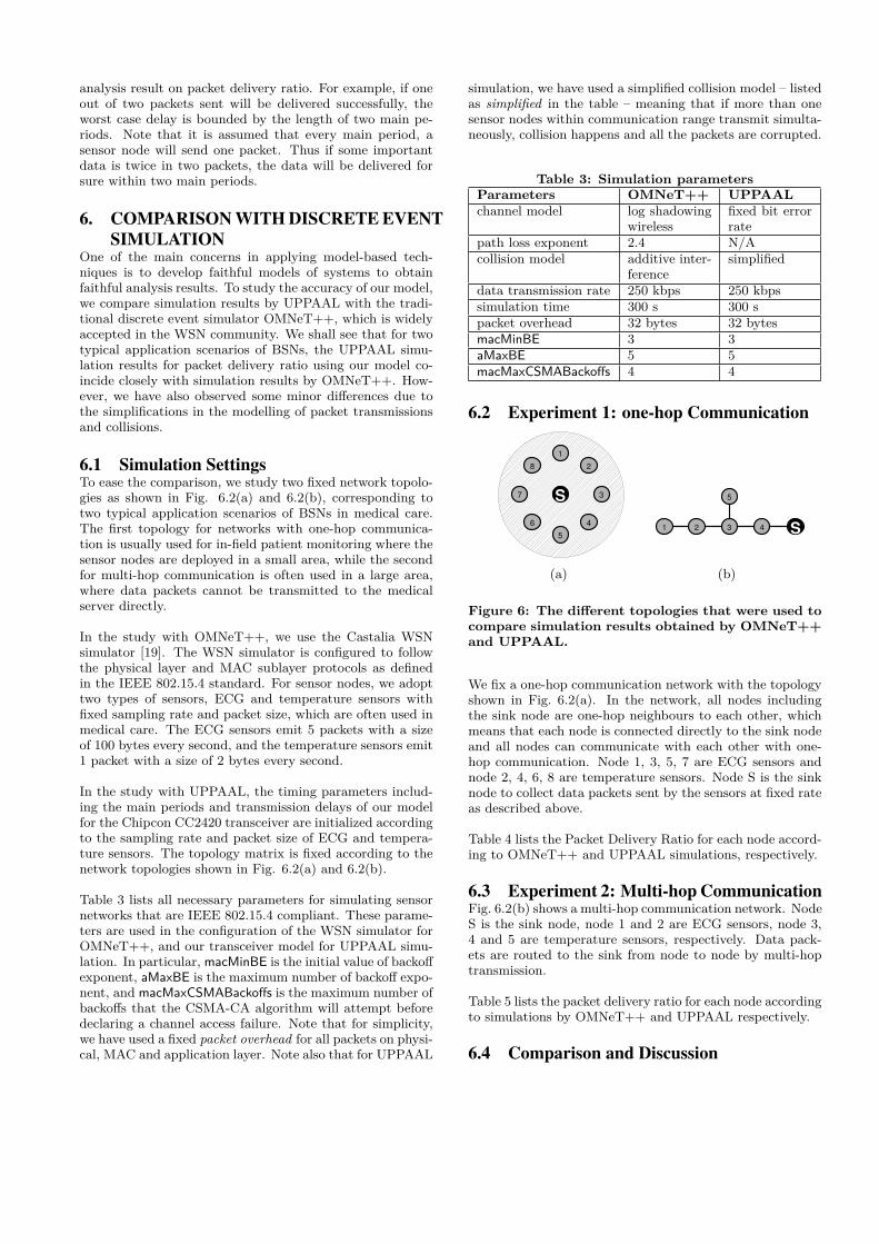
6.1 Simulation SettingsTo ease the comparison, we study two fixed network topolo-gies as shown in Fig. 6.2(a) and 6.2(b), corresponding totwo typical application scenarios of BSNs in medical care.The first topology for networks with one-hop communica-tion is usually used for in-field patient monitoring where thesensor nodes are deployed in a small area, while the secondfor multi-hop communication is often used in a large area,where data packets cannot be transmitted to the medicalserver directly.

In the study with OMNeT++, we use the Castalia WSNsimulator [19]. The WSN simulator is configured to followthe physical layer and MAC sublayer protocols as definedin the IEEE 802.15.4 standard. For sensor nodes, we adopttwo types of sensors, ECG and temperature sensors withfixed sampling rate and packet size, which are often used inmedical care. The ECG sensors emit 5 packets with a sizeof 100 bytes every second, and the temperature sensors emit1 packet with a size of 2 bytes every second.

In the study with UPPAAL, the timing parameters includ-ing the main periods and transmission delays of our modelfor the Chipcon CC2420 transceiver are initialized accordingto the sampling rate and packet size of ECG and tempera-ture sensors. The topology matrix is fixed according to thenetwork topologies shown in Fig. 6.2(a) and 6.2(b).

Table 3 lists all necessary parameters for simulating sensornetworks that are IEEE 802.15.4 compliant. These parame-ters are used in the configuration of the WSN simulator forOMNeT++, and our transceiver model for UPPAAL simu-lation. In particular, macMinBE is the initial value of backoffexponent, aMaxBE is the maximum number of backoff expo-nent, and macMaxCSMABackoffs is the maximum number ofbackoffs that the CSMA-CA algorithm will attempt beforedeclaring a channel access failure. Note that for simplicity,we have used a fixed packet overhead for all packets on physi-cal, MAC and application layer. Note also that for UPPAAL

simulation, we have used a simplified collision model – listedas simplified in the table – meaning that if more than onesensor nodes within communication range transmit simulta-neously, collision happens and all the packets are corrupted.

Table 3: Simulation parametersParameters OMNeT++ UPPAALchannel model log shadowing

wirelessfixed bit errorrate

path loss exponent 2.4 N/Acollision model additive inter-

ferencesimplified

data transmission rate 250 kbps 250 kbpssimulation time 300 s 300 spacket overhead 32 bytes 32 bytesmacMinBE 3 3aMaxBE 5 5macMaxCSMABackoffs 4 4

6.2 Experiment 1: one-hop Communication

1

4

S

5

3

2

6

8

7

(a)

1 4 S

5

32

(b)

Figure 6: The different topologies that were used tocompare simulation results obtained by OMNeT++and UPPAAL.

We fix a one-hop communication network with the topologyshown in Fig. 6.2(a). In the network, all nodes includingthe sink node are one-hop neighbours to each other, whichmeans that each node is connected directly to the sink nodeand all nodes can communicate with each other with one-hop communication. Node 1, 3, 5, 7 are ECG sensors andnode 2, 4, 6, 8 are temperature sensors. Node S is the sinknode to collect data packets sent by the sensors at fixed rateas described above.

Table 4 lists the Packet Delivery Ratio for each node accord-ing to OMNeT++ and UPPAAL simulations, respectively.

6.3 Experiment 2: Multi-hop CommunicationFig. 6.2(b) shows a multi-hop communication network. NodeS is the sink node, node 1 and 2 are ECG sensors, node 3,4 and 5 are temperature sensors, respectively. Data pack-ets are routed to the sink from node to node by multi-hoptransmission.

Table 5 lists the packet delivery ratio for each node accordingto simulations by OMNeT++ and UPPAAL respectively.

6.4 Comparison and Discussion

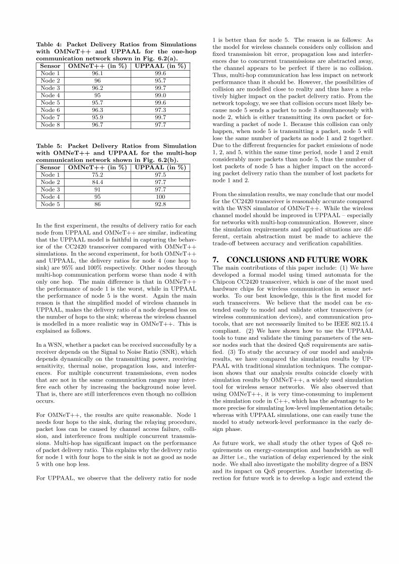
Table 4: Packet Delivery Ratios from Simulationswith OMNeT++ and UPPAAL for the one-hopcommunication network shown in Fig. 6.2(a).

Sensor OMNeT++ (in %) UPPAAL (in %)Node 1 96.1 99.6Node 2 96 95.7Node 3 96.2 99.7Node 4 95 99.0Node 5 95.7 99.6Node 6 96.3 97.3Node 7 95.9 99.7Node 8 96.7 97.7

Table 5: Packet Delivery Ratios from Simulationwith OMNeT++ and UPPAAL for the multi-hopcommunication network shown in Fig. 6.2(b).

Sensor OMNeT++ (in %) UPPAAL (in %)Node 1 75.2 97.5Node 2 84.4 97.7Node 3 91 97.7Node 4 95 100Node 5 86 92.8

In the first experiment, the results of delivery ratio for eachnode from UPPAAL and OMNeT++ are similar, indicatingthat the UPPAAL model is faithful in capturing the behav-ior of the CC2420 transceiver compared with OMNeT++simulations. In the second experiment, for both OMNeT++and UPPAAL, the delivery ratios for node 4 (one hop tosink) are 95% and 100% respectively. Other nodes throughmulti-hop communication perform worse than node 4 withonly one hop. The main difference is that in OMNeT++the performance of node 1 is the worst, while in UPPAALthe performance of node 5 is the worst. Again the mainreason is that the simplified model of wireless channels inUPPAAL, makes the delivery ratio of a node depend less onthe number of hops to the sink; whereas the wireless channelis modelled in a more realistic way in OMNeT++. This isexplained as follows.

In a WSN, whether a packet can be received successfully by areceiver depends on the Signal to Noise Ratio (SNR), whichdepends dynamically on the transmitting power, receivingsensitivity, thermal noise, propagation loss, and interfer-ences. For multiple concurrent transmissions, even nodesthat are not in the same communication ranges may inter-fere each other by increasing the background noise level.That is, there are still interferences even though no collisionoccurs.

For OMNeT++, the results are quite reasonable. Node 1needs four hops to the sink, during the relaying procedure,packet loss can be caused by channel access failure, colli-sion, and interference from multiple concurrent transmis-sions. Multi-hop has significant impact on the performanceof packet delivery ratio. This explains why the delivery ratiofor node 1 with four hops to the sink is not as good as node5 with one hop less.

For UPPAAL, we observe that the delivery ratio for node

1 is better than for node 5. The reason is as follows: Asthe model for wireless channels considers only collision andfixed transmission bit error, propagation loss and interfer-ences due to concurrent transmissions are abstracted away,the channel appears to be perfect if there is no collision.Thus, multi-hop communication has less impact on networkperformance than it should be. However, the possibilities ofcollision are modelled close to reality and thus have a rela-tively higher impact on the packet delivery ratio. From thenetwork topology, we see that collision occurs most likely be-cause node 5 sends a packet to node 3 simultaneously withnode 2, which is either transmitting its own packet or for-warding a packet of node 1. Because this collision can onlyhappen, when node 5 is transmitting a packet, node 5 willlose the same number of packets as node 1 and 2 together.Due to the different frequencies for packet emissions of node1, 2, and 5, within the same time period, node 1 and 2 emitconsiderably more packets than node 5, thus the number oflost packets of node 5 has a higher impact on the accord-ing packet delivery ratio than the number of lost packets fornode 1 and 2.

From the simulation results, we may conclude that our modelfor the CC2420 transceiver is reasonably accurate comparedwith the WSN simulator of OMNeT++. While the wirelesschannel model should be improved in UPPAAL – especiallyfor networks with multi-hop communication. However, sincethe simulation requirements and applied situations are dif-ferent, certain abstraction must be made to achieve thetrade-off between accuracy and verification capabilities.

7. CONCLUSIONS AND FUTURE WORKThe main contributions of this paper include: (1) We havedeveloped a formal model using timed automata for theChipcon CC2420 transceiver, which is one of the most usedhardware chips for wireless communication in sensor net-works. To our best knowledge, this is the first model forsuch transceivers. We believe that the model can be ex-tended easily to model and validate other transceivers (orwireless communication devices), and communication pro-tocols, that are not necessarily limited to be IEEE 802.15.4compliant. (2) We have shown how to use the UPPAALtools to tune and validate the timing parameters of the sen-sor nodes such that the desired QoS requirements are satis-fied. (3) To study the accuracy of our model and analysisresults, we have compared the simulation results by UP-PAAL with traditional simulation techniques. The compar-ison shows that our analysis results coincide closely withsimulation results by OMNeT++, a widely used simulationtool for wireless sensor networks. We also observed thatusing OMNeT++, it is very time-consuming to implementthe simulation code in C++, which has the advantage to bemore precise for simulating low-level implementation details;whereas with UPPAAL simulations, one can easily tune themodel to study network-level performance in the early de-sign phase.

As future work, we shall study the other types of QoS re-quirements on energy-consumption and bandwidth as wellas Jitter i.e., the variation of delay experienced by the sinknode. We shall also investigate the mobility degree of a BSNand its impact on QoS properties. Another interesting di-rection for future work is to develop a logic and extend the

UPPAAL model checker to fully capture QoS requirementsstudied in this paper and the other requirements on energyconsumption and network throughput for medical applica-tions [6]. The challenge is to deal with properties concern-ing mean values such as “over the life time of a network, theenergy-consumption per time unit is within a given bound”.

8. REFERENCES[1] Wireless medium access control (MAC) and physical

layer (PHY) specifications for low-rate wirelesspersonal area networks (LR-WPANs), IEEE Std.802.15.4, 2003.

[2] I. F. Akyildiz, W. Su, Y. Sankarasubramaniam, andE. Cayirci. Wireless sensor networks: a survey.Computer Networks, 38(4):393–422, 2002.

[3] G. Behrmann, A. David, and K. G. Larsen. A tutorialon uppaal. In M. Bernardo and F. Corradini, editors,Formal Methods for the Design of Real-Time Systems:4th International School on Formal Methods for theDesign of Computer, Communication, and SoftwareSystems, SFM-RT 2004, number 3185 in LNCS, pages200–236. Springer–Verlag, September 2004.

[4] J. Bengtsson and W. Yi. Timed Automata: Semantics,Algorithms and Tools. Lecture Notes on Concurrencyand Petri Nets, LNCS 3098:87–124, 2004.

[5] X. Chang. Network simulations with OPNET. InProc. of the 1999 Winter Simulation Conference(WCS’99), pages 307–314, Squaw Peak, Phoenix, AZ,December 1999.

[6] D. Chen and P. K. Varshney. QoS support in wirelesssensor networks: A survey. In Proc. of the 2004International Conference on Wireless Networks(ICWN’04), pages 227–233, Las Vegas, Nevada, USA,june 2004.

[7] Computer Science Division, University of California,Berkeley. The NS Manual, 2007.

[8] A. Fehnker, L. F. W. van Hoesel, and A. H. Mader.Modelling and verification of the lmac protocol forwireless sensor networks. Technical ReportTR-CTIT-07-09, Centre for Telematics andInformation Technology, University of Twente,Enschede, February 2007.

[9] M. Fruth. Probabilistic model checking of contentionresolution in the ieee 802.15.4 low-rate wirelesspersonal area network protocol. In T. Margaria,A. Philippou, and B. Steffen, editors, Proceedings ofthe 2nd International Symposium on LeveragingApplications of Formal Methods, Verification andValidation (ISoLA 2006), Paphos, Cyprus, November2006.

[10] L. Girod, T. Stathopoulos, N. Ramanathan, J. Elson,D. Estrin, E. Osterweil, and T. Schoellhammer. Asystem for simulation, emulation, and deployment ofheterogeneous sensor networks. In Proc. of the 2ndInternational Conference on Embedded NetworkedSensor Systems (SenSys’04), pages 201–213,Baltimore, MD, USA, November 2004.

[11] Y. Guang-Zhong, editor. Body Sensor Networks.Springer, New York, 2006.

[12] O. Landsiedel, K. Wehrle, B. Titzer, and J. Palsberg.Enabling detailed modeling and analysis of sensornetworks. Praxis der Informationsverarbeitung und

Kommunikation, 28(2):101–106, April 2005.[13] K. G. Larsen, P. Pettersson, and W. Yi. Uppaal in a

Nutshell. Int. Journal on Software Tools forTechnology Transfer, 1(1–2):134–152, Oct. 1997.

[14] P. Levis, N. Lee, M. Welsh, and D. Culler. TOSSIM:accurate and scalable simulation of entire tinyosapplications. In Proc. of the 1st internationalconference on Embedded networked sensor systems(SenSys’03), pages 126–137, Los Angeles, California,USA, November 2003.

[15] X. Liang, B. Østvold, W. Leister, and I. Balasingham.Credo: Modeling and analysis of evolutionarystructures for distributed services – user drivenrequirements, March 2007. Diliverable D6.1, EU ISTproject, number 33826.

[16] P. C. Olveczky and S. Thorvaldsen. Formal modelingand analysis of the OGDC wireless sensor networkalgorithm in Real-Time Maude. In Proc. of the 9thIFIP International Conference on Formal Methods forOpen Object-Based Distributed Systems (FMOODS’07), pages 122–140, Paphos, Cyprus, Juni 2007.

[17] F. Osterlind, A. Dunkels, J. Eriksson, and N. F. T.Voigt. Cross-level sensor network simulation withCOOJA. In Proc. of the 31st IEEE Conference onLocal Computer Networks, pages 641–648, Tampa,Florida, USA, November 2006.

[18] S. Park, A. Savvides, and M. B. Srivastava. SensorSim:a simulation framework for sensor networks. In Proc.of the 3rd ACM international workshop on Modeling,analysis and simulation of wireless and mobile systems(ACM MSWiM 2000), pages 104–111, Boston,Massachusetts, USA, August 2000.

[19] H. N. Pham, D. Pediaditakis, and A. Boulis. Fromsimulation to real deployments in WSN and back. InProc. of the 8th IEEE International Symposium on aWorld of Wireless, Mobile and Multimedia Networks(WoWMoM’07), pages 1–6, Helsinki, Finland, June2007.

[20] J. Polley, D. Blazakis, J. McGee, D.Rusk, andJ. Baras. ATEMU: a fine-grained sensor networksimulator. In Proc. of the 1st IEEE CommunicationsSociety Conference on Sensor and Ad HocCommunications and Networks (SECON’04), pages145–152, Los Angeles, California, USA, October 2004.

[21] Scalable Network Technologies, Inc. QualNet 3.9.5User’s Guide, 2006.

[22] Texas Instruments Incorporated, Dallas, Texas, USA.2.4 GHz IEEE 802.15.4 / ZigBee-Ready RFTransceiver (Rev. B), CC2420 data sheet, March 2007.

[23] B. L. Titzer, D. K. Lee, and J. Palsberg. Avrora:scalable sensor network simulation with precisetiming. In Proc. of the 4th International Symposiumon Information Processing in Sensor Networks(IPSN’05), pages 477–482, Los Angeles, California,USA, April 2005.

[24] A. Varga. The OMNeT++ discrete event simulationsystem. In Proc. of the 15th European SimulationMulticonference (ESM’01), pages 112–118, Prague,Czech Republic, Juni 2001.

[25] H. Zhang and J. C. Hou. Maintaining sensing coverageand connectivity in large sensor network. Wireless AdHoc and Sensor Networks, 1(1-2):89–123, jan 2005.

APPENDIXA. FURTHER DESCRIPTION OF THE

TRANSCEIVER MODELA.1 States

� Initial_delay: In a real system not all nodes areturned on at the same time; thus we have randomlychosen an initial delay for every node before the firstactive period. This is to model the initialization of asensor node.

� RX_SFD_SEARCH: In this state, the transceiver is listen-ing to incoming signals.

� PreRX: A node that starts packet transmission uses abroadcasting channel provided by UPPAAL to informnodes in state RX_SFD_SEARCH of a beginning trans-mission. UPPAAL does not allow to broadcast onlyto a limited number of nodes, thus the PreRX-state isneeded. If the notification (i.e. the broadcast) comesfrom a node out of range, it will be ignored.

� RX_FRAME: A node will enter this state when it receivesa valid signal, and then it will leave the state if thewhole packet is successfully transmitted or corrupted.

� PowerDown: This state represents the power saving modeof the transceiver.

� Backoff: In this state, a node waits for a random back-off concerning the IEEE 802.15.4 CSMA-CA.

� PreTX: This state is to model that the transceiver isperforming the clear channel assessment.

� TX_CALIBRATE: This state models the delay that occursin the real hardware to set up a transmission.

� TX_PREAMBLE: The frame preamble is transmitted dur-ing this state. It is modelled by the broadcast channelmentioned above.

� TX_FRAME: In this state, the transceiver is transmittingthe payload of a packet.

A.2 Constants and Parameters� ID: Each node has a unique ID. This ID is used to

identify messages progressing through the network.� P_M: It denotes the main period of a sensor node.� P_W: It denotes the active period of a sensor node.� D: In a BSN, nodes are usually not activated at exactly

the same time. This is modelled using an initial delayD.

� P_S[]: This array contains the duration of a transmis-sion for every packet type. It can be derived from thepacket size.

� BACK[]: The bounds for the length of a backoff perioddepend on the number of re-transmissions, accordingto the IEEE 802.15.4 standard.

� MAX_BO: The maximum number of backoff periods be-fore declaring a channel access failure.

A.3 Global Variables� buffer[]: This is the buffer for outgoing packets of a

node. It is globally accessible for statistical purposes.

� signal[]: This array models the incoming signal of anode. It is set by the sending nodes in range. If it is0, it indicates that no node in range is transmitting.If two nodes in range are transmitting, the value forthe corresponding receiving node is set to be negative.Otherwise it is set to the packet that is being transmit-ted.

� topology[][]: This is the topology matrix.

� ignore[X][Y]: This is to model the controlled dynamicrouting scheme with acknowledgement. Each elementmay have three values: 0; 1 and 2 denoting the threesituations respectively: node X has not received packetY , node X has received Y for forwarding, and node Xhas forwarded Y and it has been acknowledged.

� meta periods[]: This array contains a counter for thenumber of main periods of each sensor node. In general,its value is equivalent to the number of packets emittedby a node.

� meta received[]: This array contains counters for thenumber of different packets received by the sink.

A.4 Local Variables and Clocks� Clock X: It is used to model the main period of a sensor

node.

� Clock Y: It is used to model the transmission times forpackets, the back-off period, and the timeout period foracknowledgements.

� bound: If a node waits for an acknowledgement, thisvariable is set to the period for the timeout. Otherwiseit is set to be the main period of a sensor node.

� tmp: This variable is used to store the ID of the sendingnode during packet reception.

� tmp_sig: This variable is used to store the incommingsignal during packet reception.

� bo_cnt: This is a counter for the number of passedbackoff periods, i.e. the number of failed transmissionattempts.

A.5 Channels� start[]: This is a broadcast channel to model the be-

ginning of a packet transmission.

� stop[]: This is a broadcast channel to model the endof a packet transmission.

� go: This is an urgent channel to model urgent transi-tions.

A.6 Functions� send: This function is called, when a node wants to

start a packet transmission. It check through the topol-ogy matrix and updates the incoming signals of allnodes in transmission range. In addition the func-tion implements the functionality needed to model col-lisions.

� reset_signal: This function is the complement to thesend-function. It sets back the value of the incomingsignal for each node in transmission range.

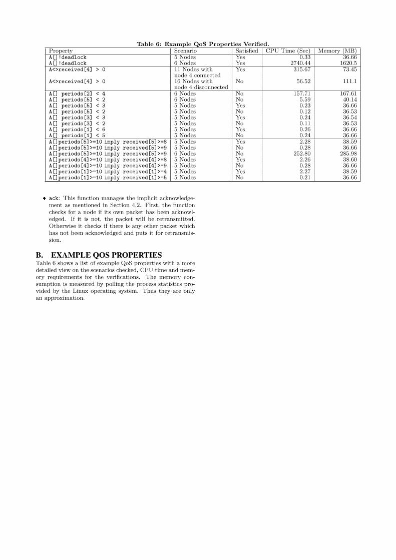
Table 6: Example QoS Properties Verified.Property Scenario Satisfied CPU Time (Sec) Memory (MB)A[]!deadlock 5 Nodes Yes 0.33 36.66A[]!deadlock 6 Nodes Yes 2740.44 1620.5A<>received[4] > 0 11 Nodes with Yes 315.67 73.45

node 4 connectedA<>received[4] > 0 16 Nodes with No 56.52 111.1

node 4 disconnectedA[] periods[2] < 4 6 Nodes No 157.71 167.61A[] periods[5] < 2 6 Nodes No 5.59 40.14A[] periods[5] < 3 5 Nodes Yes 0.23 36.66A[] periods[5] < 2 5 Nodes No 0.12 36.53A[] periods[3] < 3 5 Nodes Yes 0.24 36.54A[] periods[3] < 2 5 Nodes No 0.11 36.53A[] periods[1] < 6 5 Nodes Yes 0.26 36.66A[] periods[1] < 5 5 Nodes No 0.24 36.66A[]periods[5]>=10 imply received[5]>=8 5 Nodes Yes 2.28 38.59A[]periods[5]>=10 imply received[5]>=9 5 Nodes No 0.28 36.66A[]periods[5]>=10 imply received[5]>=9 6 Nodes No 252.80 285.98A[]periods[4]>=10 imply received[4]>=8 5 Nodes Yes 2.26 38.60A[]periods[4]>=10 imply received[4]>=9 5 Nodes No 0.28 36.66A[]periods[1]>=10 imply received[1]>=4 5 Nodes Yes 2.27 38.59A[]periods[1]>=10 imply received[1]>=5 5 Nodes No 0.21 36.66

� ack: This function manages the implicit acknowledge-ment as mentioned in Section 4.2. First, the functionchecks for a node if its own packet has been acknowl-edged. If it is not, the packet will be retransmitted.Otherwise it checks if there is any other packet whichhas not been acknowledged and puts it for retransmis-sion.

B. EXAMPLE QOS PROPERTIESTable 6 shows a list of example QoS properties with a moredetailed view on the scenarios checked, CPU time and mem-ory requirements for the verifications. The memory con-sumption is measured by polling the process statistics pro-vided by the Linux operating system. Thus they are onlyan approximation.