Model-based Reasoning

‘Traditional’ knowledge systems:

Rule based (heuristic rules)if conditions then actions/conclusions fi

...

Reasoning:forward chaining: reasoning from facts toconclusionsbackward chaining: reasoning from goals to facts

Recent: business rules

Model-based systems: reasoning with understandablemodel, i.e., they have intuitive semantics

– p. 1/30

Heuristic rules and their disadvantages

Problem solving based on heuristic rules:

category

category category category

category(feature1 ∧ · · · ∧ featuren)

→ category

Disadvantages:

no use of knowledge about structure and workings

knowledge maintenance and updating is hard

– p. 2/30

Model use

problemdomain

declarativeknowledge

knowledgebase

problemsolving method

inferenceengine

Models:usually designed for handling multiple problems⇒reusecapture instantaneous behaviour, temporalbehaviour, structure

Methods: diagnosis, decision making, prediction,planning

– p. 3/30

Medical diagnosis of facial palsy

internalmeatus

facial canal

IV: herpes meatus

V: deafness

III: hyperacusis

II: taste

I: drooping mouth angle

level

n. stapedius

Diagnosis:Symptoms-leveli+1 =

Symptoms-leveli ∪New-symptoms

– p. 4/30

Drilling Automation for Mars

Autonomous drillwith sensors

Fault diagnosis

– p. 5/30

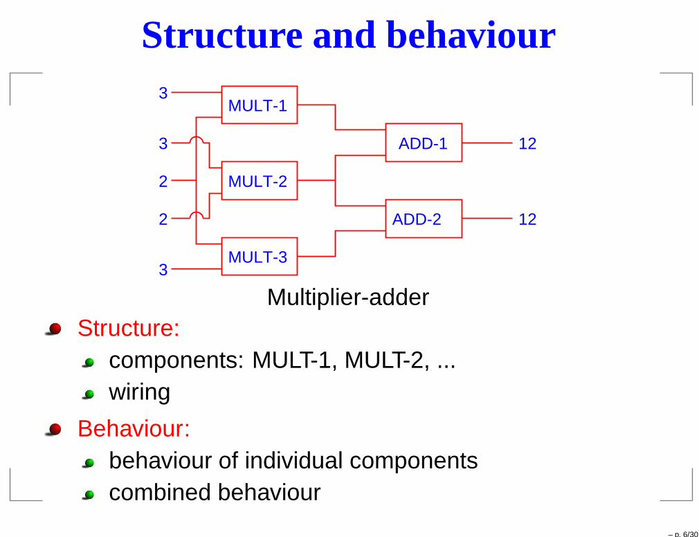
Structure and behaviour

MULT-1

MULT-2

ADD-1

ADD-2

3

3

2

2

3

12

12

MULT-3

Multiplier-adderStructure:

components: MULT-1, MULT-2, ...wiring

Behaviour:behaviour of individual componentscombined behaviour

– p. 6/30

Method: model-based diagnosis

system

comparison

diction‘

pre−

ation

observ−actual

behaviourstructure/model of

behaviourpredicted

observedbehaviour

Model: representation of normal or abnormal behaviourand, possibly, internal structure

Formalisation:consistency-based diagnosis, andabductive diagnosis

– p. 7/30

OCC’M

– p. 8/30

Consistency-based diagnosis

ation

observ−

predicted

discrepancy

observedbehaviour

diction

normalmodel ofstructure/behaviour

actualsystem

behaviour

pre−

Difference between predicted behaviour and observedbehaviour⇒ defect!

Originators:R. Reiter, “A Theory of diagnosis from first principles”, Artificial Intelligence, vol. 32,57–95, 1987.

J. de Kleer, A.K. Macworth, and R. Reiter, “Characterising diagnoses and systems”,Artificial Intelligence, vol. 52, 197–222, 1992.

– p. 9/30

Normal behaviour

M1

M2

M3

A1

A 2

SYStem specification SYS = (SD,COMPS):

Components that may be defective (faulty):COMPS = {M1,M2,M3, A1, A2}

SD (System Description):generic description of component behaviour (whatthe component does)declaration of components: MUL(M1), ADD(A1)

connection between components

– p. 10/30

Normal behaviour: formalM1

M2

M3

A1

A 2

SYStem specification SYS = (SD,COMPS):SD (System Description):∀x(MUL(x)→ in1(x)× in2(x) = out(x))∀x(ADD(x)→ in1(x) + in2(x) = out(x))

MUL(M1),MUL(M2),MUL(M3),ADD(A1),ADD(A2)in1(A1) = out(M1), in2(A1) = out(M2)in1(A2) = out(M2), in2(A2) = out(M3)

COMPS = {M1,M2,M3, A1, A2}

– p. 11/30

Ab predicateAb(c): component c is abnormal

¬Ab(c): component c is not abnormal, i.e. normal

Example (Inverter I):

I1 0[1]

SD = {∀x((INV(x) ∧ ¬Ab(x))→ ¬(out(x) = in(x))), INV(I)}

Input: in(I) = 1; observed output: out(I) = 1

SD ∪ {in(I) = 1, out(I) = 1} ∪ {¬Ab(I)} � ⊥

SD ∪ {in(I) = 1, out(I) = 1} ∪ {Ab(I)} 2 ⊥

(assumption that I is (ab)normal is (in)consistent)

– p. 12/30

Normal behaviour formalM1

M2

M3

A1

A 2

3

3

2

2

3

12

12

SYStem specification SYS = (SD, COMPS):SD (System Description):∀x((MUL(x) ∧ ¬Ab(x))→ in1(x)× in2(x) = out(x))∀x((ADD(x) ∧ ¬Ab(x))→ in1(x) + in2(x) = out(x))

MUL(M1),MUL(M2),MUL(M3),ADD(A1),ADD(A2)in1(A1) = out(M1), in2(A1) = out(M2)in1(A2) = out(M2), in2(A2) = out(M3)

COMPS = {M1,M2,M3, A1, A2}

– p. 13/30

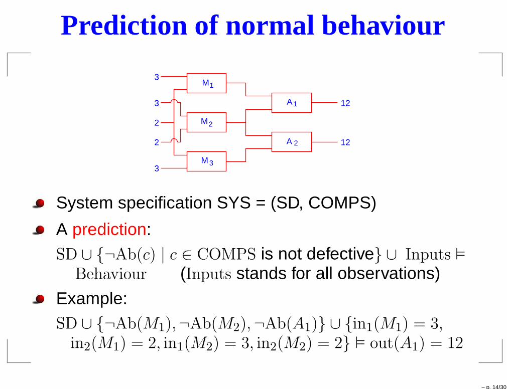
Prediction of normal behaviour

M1

M2

M3

A1

A 2

3

3

2

2

3

12

12

System specification SYS = (SD, COMPS)

A prediction:SD ∪ {¬Ab(c) | c ∈ COMPS is not defective} ∪ Inputs �

Behaviour (Inputs stands for all observations)

Example:SD ∪ {¬Ab(M1),¬Ab(M2),¬Ab(A1)} ∪ {in1(M1) = 3,

in2(M1) = 2, in1(M2) = 3, in2(M2) = 2} � out(A1) = 12

– p. 14/30

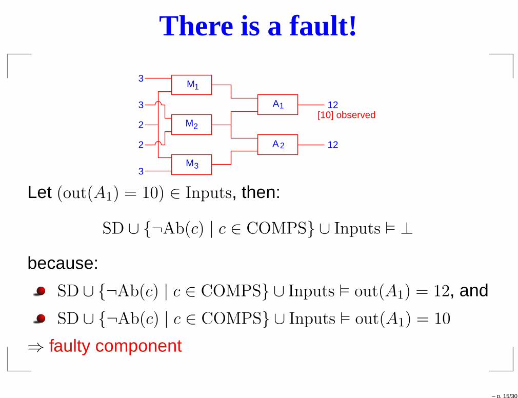
There is a fault!

M1

M2

M3

A1

A2

3

3

2

2

3

12

12[10] observed

Let (out(A1) = 10) ∈ Inputs, then:

SD ∪ {¬Ab(c) | c ∈ COMPS} ∪ Inputs � ⊥

because:

SD ∪ {¬Ab(c) | c ∈ COMPS} ∪ Inputs � out(A1) = 12, and

SD ∪ {¬Ab(c) | c ∈ COMPS} ∪ Inputs � out(A1) = 10

⇒ faulty component

– p. 15/30

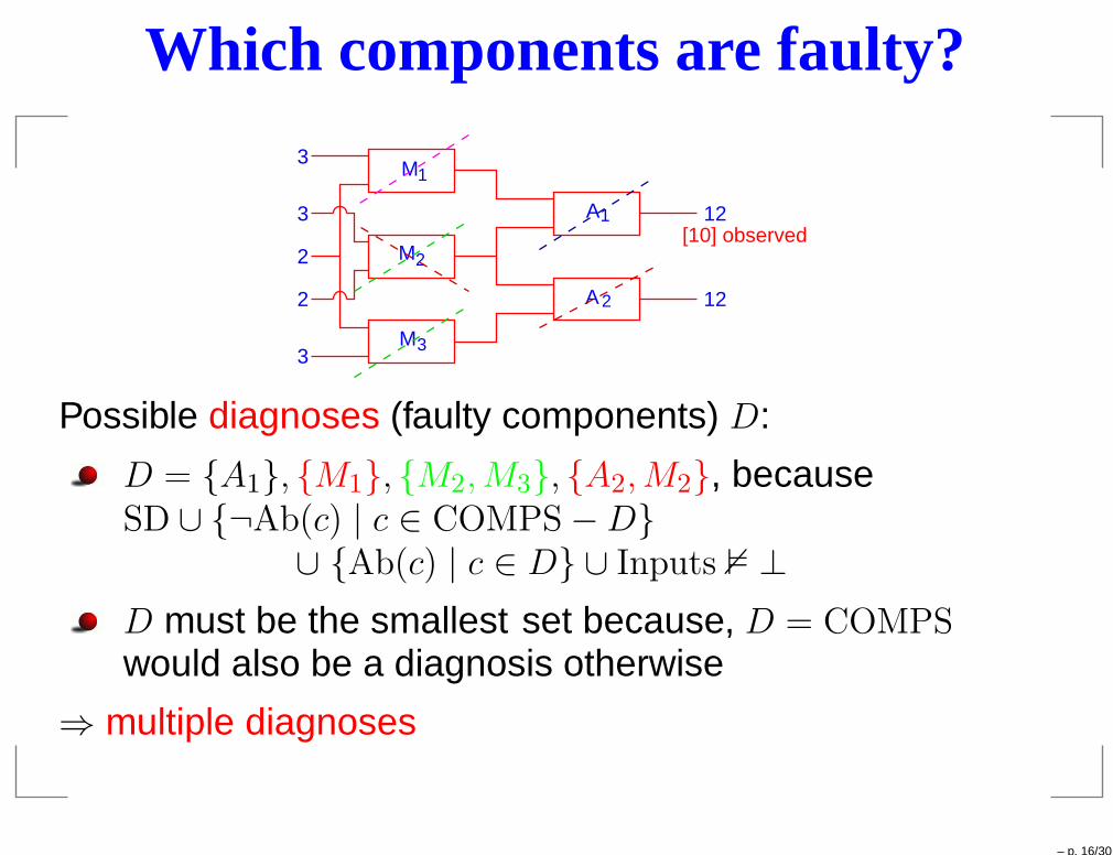
Which components are faulty?

M1

M2

M3

A1

A2

3

3

2

2

3

12

12[10] observed

Possible diagnoses (faulty components) D:

D = {A1}, {M1}, {M2,M3}, {A2,M2}, becauseSD ∪ {¬Ab(c) | c ∈ COMPS−D}

∪ {Ab(c) | c ∈ D} ∪ Inputs 2 ⊥

D must be the smallest set because, D = COMPSwould also be a diagnosis otherwise

⇒ multiple diagnoses

– p. 16/30

Diagnostic problem

System specification SYS = (SD, COMPS)

Diagnostic problem DP = (SYS, OBS), with OBS a set ofobservations

A diagnosis D: smallest (subset minimal) set ofcomponents, such that

SD ∪ OBS ∪ {Ab(c) | c ∈ D} ∪ {¬Ab(c) | c ∈ COMPS−D}

is consistent

Example:OBS = {in1(M1) = 3, in2(M1) = 2, in1(M2) = 3, in2(M2) = 2,

in1(M3) = 2, in2(M3) = 3, out(A1) = 10, out(A2) = 12}

– p. 17/30

AlgorithmsEnumerate all diagnoses: #P complete (NP hard forenumeration):

Ab(A1) ∧ ¬Ab(A2) ∧ ¬Ab(M1) ∧ ¬Ab(M2) ∧ ¬Ab(M3)Ab(A1) ∧ Ab(A2) ∧ ¬Ab(M1) ∧ ¬Ab(M2) ∧ ¬Ab(M3)Ab(A1) ∧ Ab(A2) ∧ Ab(M1) ∧ ¬Ab(M2) ∧ ¬Ab(M3)

...

Heuristic methods:hitting set algoritme (Reiter)assumption-based truth maintenance system(ATMS, De Kleer)

Restrictions: for example, only maximally 2 defects,then complexity upperbound

Basic problem: which idea should underly such algorithms?

– p. 18/30

Conflict set

Let CS ⊆ COMPS be a set of components, then CS is called aconflict set iff

SD ∪ OBS ∪ {¬Ab(c) | c ∈ CS}

is inconsistent (SD ∪ OBS ∪ {¬Ab(c) | c ∈ CS} � ⊥)

Proposition: For each D ⊆ COMPS that is a diagnosis andeach conflict set CS it holds that: D ∩ CS 6= ∅

Proof: SD ∪ OBS ∪ {¬Ab(c) | c ∈ COMPS−D} 2 ⊥, with Dsubset minimal⇒ COMPS−D is subset maximal, hence

SD ∪ OBS ∪ {¬Ab(c) | c ∈ COMPS−D} ∪ {¬Ab(c′)}︸ ︷︷ ︸

CS

� ⊥

for c′ in CS

– p. 19/30

Basic ideas: hitting sets

Determine conflict sets of the diagnostic problem DP

Each conflict set CS has at least one element incommon with a diagnosis D:

D = {c1, c2, . . . , cm}/ \

CS1 = {. . . , c1, . . .} CSm = {. . . , cm, . . .}

Compute so-called hitting sets:Let F be a set of sets, andH ⊆

⋃

S∈FS,

H is a hitting set if for all S ∈ F : H ∩ S 6= ∅

Example: F = {{1, 2}, {3, 4}}, then H = {2, 4} is a(non-unique) hitting set (H = {1, 3} is also a hitting set)

– p. 20/30

Diagnosis as hitting set

Theorem: D is a diagnosis for diagnostic problemDP = (SYS, OBS) iff D is a minimal hitting set for all conflictsets of DP

Proof (sketch):

Prop. page 19: for all conflict sets CS: CS ∩D 6= ∅.Thus, D is a hitting set

D is also a minimal hitting set, as COMPS−D is noconflict set, whereas {c} ∪ (COMPS−D) is a conflict setfor any c ∈ D

– p. 21/30

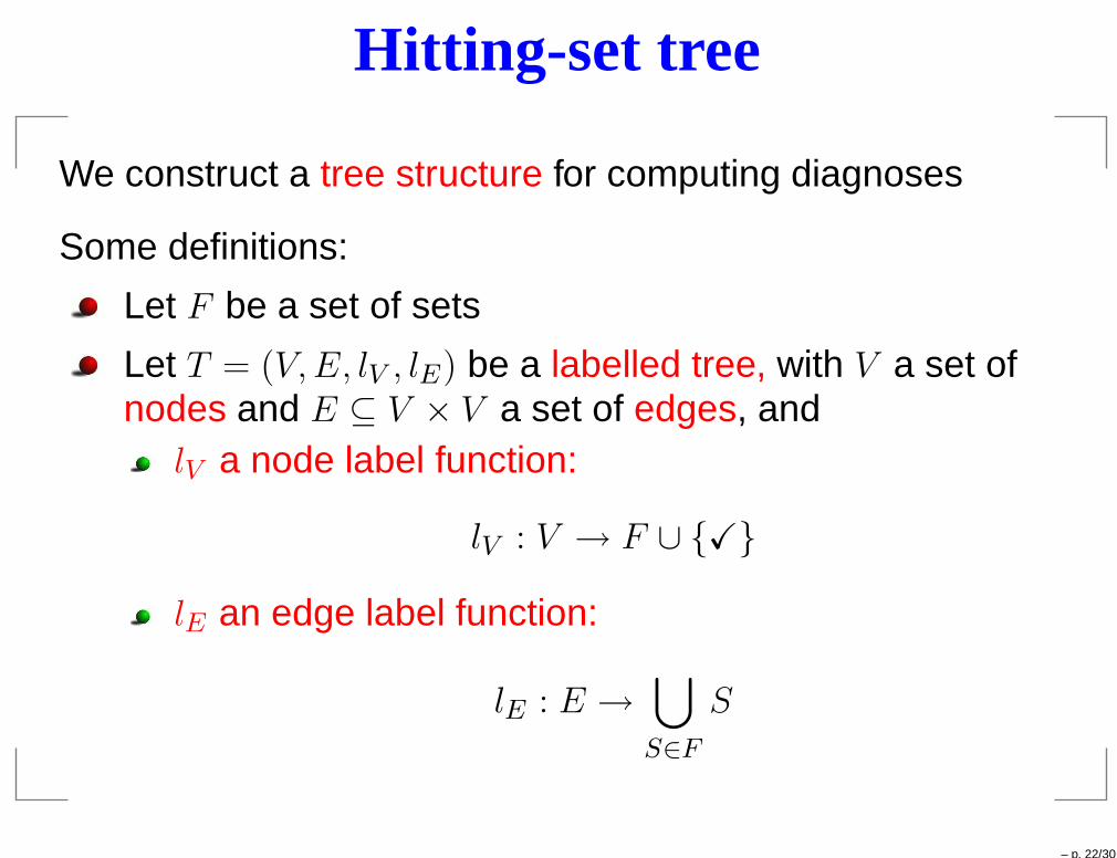
Hitting-set tree

We construct a tree structure for computing diagnoses

Some definitions:

Let F be a set of sets

Let T = (V,E, lV , lE) be a labelled tree, with V a set ofnodes and E ⊆ V × V a set of edges, and

lV a node label function:

lV : V → F ∪ {X}

lE an edge label function:

lE : E →⋃

S∈F

S

– p. 22/30

Node label function

Let F be a set of sets:

lV a node label function:

lV : V → F ∪ {X}

with

lV (v) =

{

S if S ∈ F , S 6= ∅

X otherwise

Example: F = {{1, 2}, {4, 5}}

Nodes V = {u, v, w}

lV (u) = {1, 2}, lV (v) = {4, 5}, and lV (w) = X

– p. 23/30

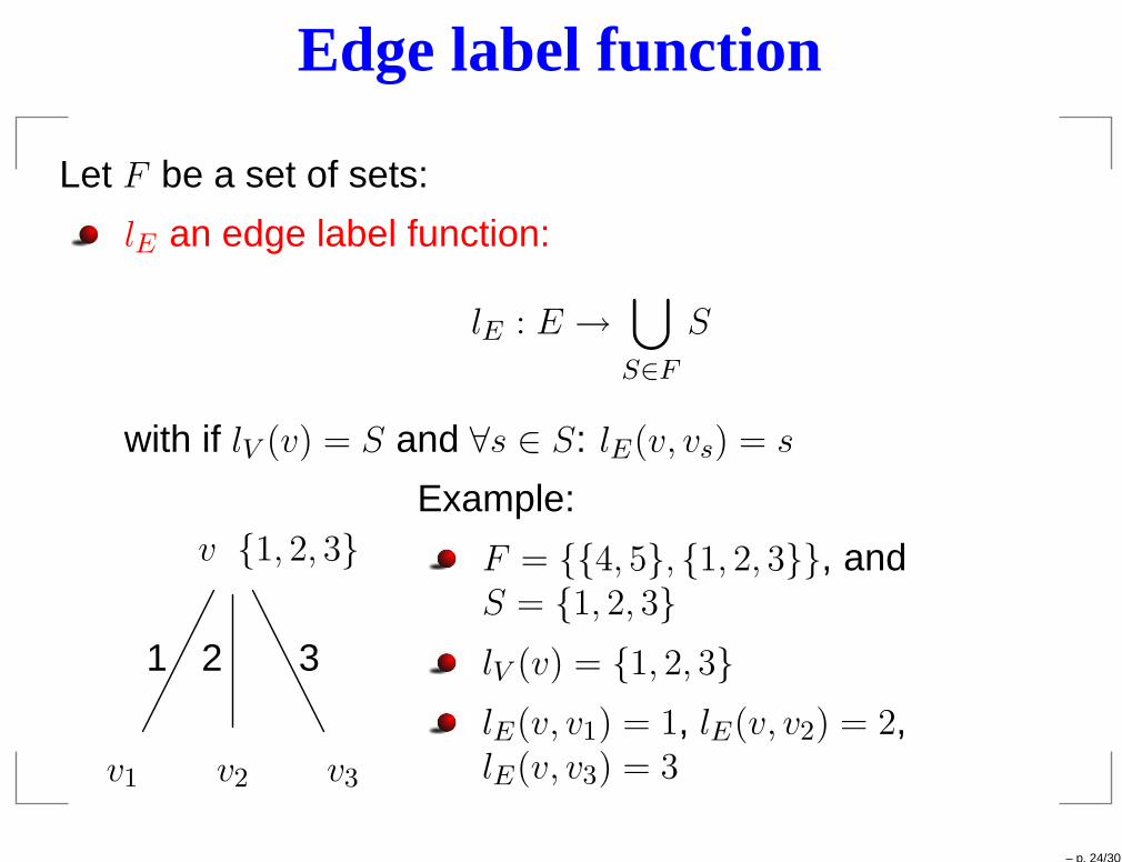
Edge label function

Let F be a set of sets:

lE an edge label function:

lE : E →⋃

S∈F

S

with if lV (v) = S and ∀s ∈ S: lE(v, vs) = s

v {1, 2, 3}

v2v1 v3

21 3

Example:

F = {{4, 5}, {1, 2, 3}}, andS = {1, 2, 3}

lV (v) = {1, 2, 3}

lE(v, v1) = 1, lE(v, v2) = 2,lE(v, v3) = 3

– p. 24/30

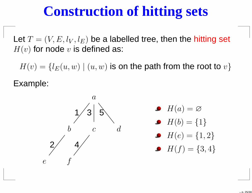
Construction of hitting sets

Let T = (V,E, lV , lE) be a labelled tree, then the hitting setH(v) for node v is defined as:

H(v) = {lE(u,w) | (u,w) is on the path from the root to v}

Example:

a

cb d

e f

31 5

2 4

H(a) = ∅

H(b) = {1}

H(e) = {1, 2}

H(f) = {3, 4}

– p. 25/30

Hitting-set algorithm

F is the set of conflict sets, which is initially empty

Let node vs be a child of node v, then lV (vs) = CS ifthere is exists a CS ∈ F with

CS ∩H(vs) = ∅

(CS is not yet covered by H(vs) and we have to extendthe path)

If no suitable CS ∈ F , call logical reasoning program TP:Call: TP(SD, COMPS−H(vs), OBS)Returns: conflict set CS if

SD ∪ OBS ∪ {¬Ab(c) | c ∈ COMPS−H(vs)} � ⊥, withCS ∩H(vs) = ∅ and CS ⊆ COMPS−H(vs)

otherwise, X (consistent)

– p. 26/30

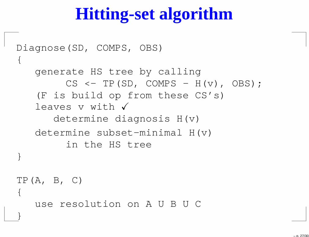
Hitting-set algorithm

Diagnose(SD, COMPS, OBS){

generate HS tree by callingCS <- TP(SD, COMPS - H(v), OBS);

(F is build op from these CS’s)leaves v with X

determine diagnosis H(v)

determine subset-minimal H(v)in the HS tree

}

TP(A, B, C){

use resolution on A U B U C}

– p. 27/30

Example: full-adder

X1

A1

A2

X2

O1

10

1

0 predicted[1] observed

1 predicted[0] observed

SD:∀x((ANDG(x) ∧ ¬Ab(x))→ (out(x) = in1(x) ∧ in2(x)))∀x((ORG(x) ∧ ¬Ab(x))→ (out(x) = in1(x) ∨ in2(x)))

...ORG(O1), ANDG(A1), XORG(X1), . . .

COMPS = {A1, A2, X1, X2, O1}

– p. 28/30

Example HS tree

v1 {X1, X2}

v2 v3 {X1, A2, O1}

v4 v5 v6

X

X X

X1 X2

X1 A2 O1

1. CS1 ← TP(SD, COMPS, OBS);CS1 ← {X1, X2}

2. CS2 ← TP(SD, COMPS −{X1}, OBS);CS2 ← X (diagnosis found)

3. CS3 ← TP(SD, COMPS −{X2}, OBS);CS3 ← {X1, A2, O1}

4....

Diagnoses D: {X1}, {X2, A2}, {X2, O1}(note that {X2, X1} not subset minimal)

– p. 29/30

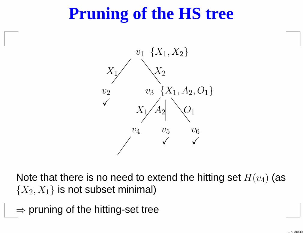
Pruning of the HS tree

v1 {X1, X2}

v2 v3 {X1, A2, O1}

v4 v5 v6

X

X X

X1 X2

X1 A2 O1

Note that there is no need to extend the hitting set H(v4) (as{X2, X1} is not subset minimal)

⇒ pruning of the hitting-set tree

– p. 30/30