Model-Based Geostatistics for

Prevalence Mapping in Low-Resource Settings

Peter J Diggle1,2 and Emanuele Giorgi1

Lancaster University1 and University of Liverpool2

combininghealth information,

computation and statistics

CHICAS

References

Diggle, P.J., Moyeed, R.A. and Tawn, J.A. (1998). Model-based Geostatistics(with Discussion). Applied Statistics 47 299–350.

Diggle, P.J., Thomson, M.C., Christensen, O.F., Rowlingson, B., Obsomer, V.,Gardon, J., Wanji, S., Takougang, I., Enyong, P., Kamgno, J., Remme, H.,Boussinesq, M. and Molyneux, D.H. (2007). Spatial modelling and predictionof Loa loa risk: decision making under uncertainty. Annals of Tropical Medicineand Parasitology, 101, 499–509.

Giorgi, E., Sesay, S.S., Terlouw, D.J. and Diggle, P.J. (2014). Combining datafrom multiple spatially referenced prevalence surveys using generalized lineargeostatistical models. Journal of the Royal Statistical Society A (to appear)

Rodrigues, A. and Diggle, P.J. (2010). A class of convolution-based models forspatio-temporal processes with non-separable covariance structure.Scandinavian Journal of Statistics, 37, 553–567.

Zoure, H.G.M., Noma, M., Tekle, A.H., Amazigo, U.V., Diggle, P.J., Giorgi, E.and Remme, J.H.F. (2014). The geographic distribution of onchocerciasis inthe 20 participating countries of the African Programme for OnchocerciasisControl: 2. Pre-control endemicity Levels and estimated number infected.Parasites and Vectors, 7, 326

Acknowledgements

CHICAS, Lancaster: Ole Christensen, Barry Rowlingson, MichelleStanton, Ben Taylor, Rachel Tribbick

MLW, Blantyre, Malawi Sanie Sesay, Anja Terlouw

APOC, Ouagadougou: Hans Remme, Honorat Zoure, Sam Wanji

IRI, Columbia University: Madeleine Thomson

...and many others

Outline

introduction

general remarks on statistical modelling

the standard binomial geostatistical model: Loa loa

low-rank approximations: river blindness

combining data from multiple surveys: malaria

spatially structured zero-inflation: river blindness re-visited

implementation

closing remarks

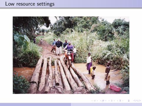
Low resource settings

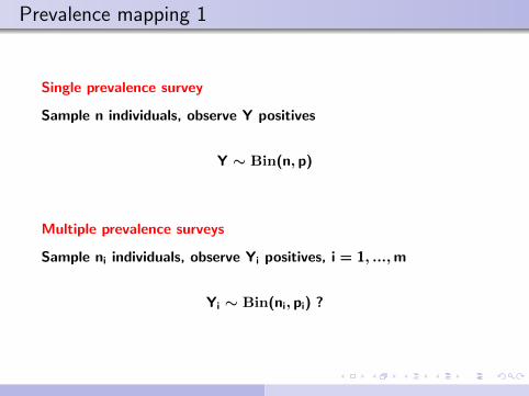
Prevalence mapping 1

Single prevalence survey

Sample n individuals, observe Y positives

Y ∼ Bin(n, p)

Multiple prevalence surveys

Sample ni individuals, observe Yi positives, i = 1, ...,m

Yi ∼ Bin(ni, pi) ?

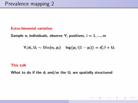
Prevalence mapping 2

Extra-binomial variation

Sample ni individuals, observe Yi positives, i = 1, ...,m

Yi|di,Ui ∼ Bin(ni, pi) log{pi/(1− pi)} = d′iβ + Ui

This talk

What to do if the di and/or the Ui are spatially structured

Geostatistics

traditionally, a self-contained methodology for spatialprediction, developed at Ecole des Mines,Fontainebleau, France

nowadays, that part of spatial statistics which isconcerned with data obtained by spatially discretesampling of a spatially continuous process

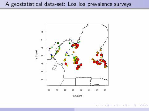
A geostatistical data-set: Loa loa prevalence surveys

8 9 10 11 12 13 14 15

23

45

67

8

X Coord

Y C

oord

Model-based Geostatistics(Diggle, Moyeed and Tawn, 1998)

the application of general principles of statisticalmodelling and inference to geostatistical problems

− formulate a model for the data

− use likelihood-based methods of inference

− answer the scientific question

Statistical modelling principles

models are devices to answer questions

models should:

be not demonstrably inconsistent with the data;

incorporate the underlying science, where this is well understood

be as simple as possible, within the above constraints

“Too many notes, Mozart”

Emperor Joseph II

“Only as many as there needed to be”

Mozart (apochryphal?)

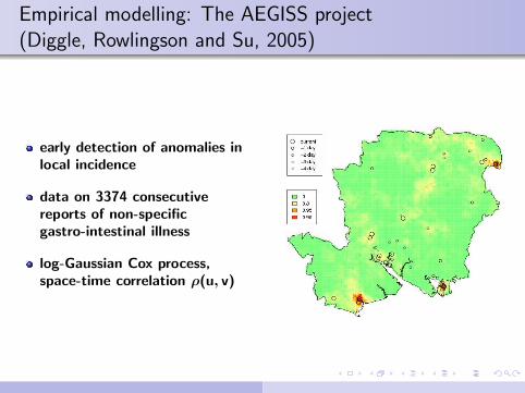
Empirical modelling: The AEGISS project(Diggle, Rowlingson and Su, 2005)

early detection of anomalies inlocal incidence

data on 3374 consecutivereports of non-specificgastro-intestinal illness

log-Gaussian Cox process,space-time correlation ρ(u, v)

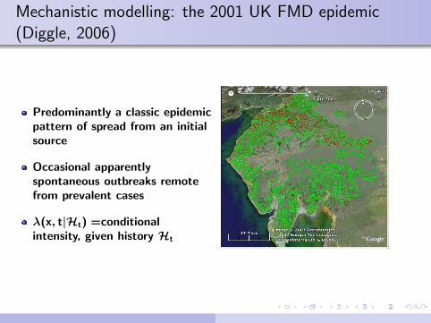
Mechanistic modelling: the 2001 UK FMD epidemic(Diggle, 2006)

Predominantly a classic epidemicpattern of spread from an initialsource

Occasional apparentlyspontaneous outbreaks remotefrom prevalent cases

λ(x, t|Ht) =conditionalintensity, given history Ht

Onchocerciasis (River Blindness)

APOC

AfricanProgramme forOnchocerciasisControl

“river blindness” – endemic in wet tropical regions

donation programme of mass treatment with ivermectin

approximately 60 million treatments to date, in 19 countries

serious adverse reactions experienced by some patients highlyco-infected with Loa loa parasites

precautionary measures put in place before masstreatment in areas of high Loa loa prevalence

http://www.who.int/pbd/blindness/onchocerciasis/en/

Loa loa young

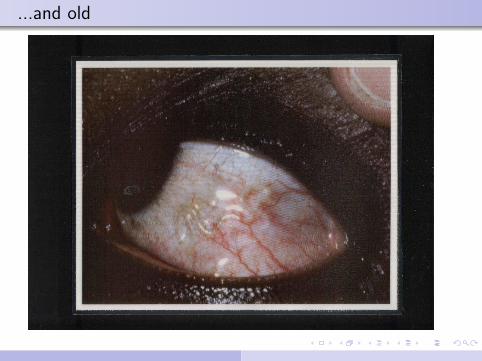
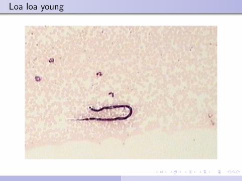
...and old

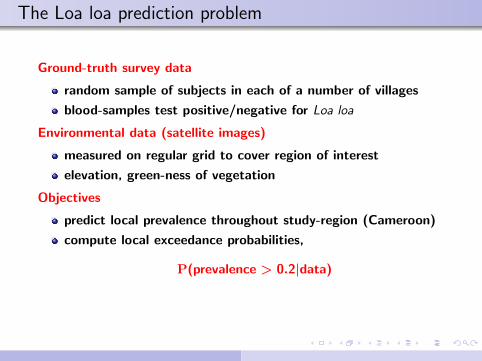
The Loa loa prediction problem

Ground-truth survey data

random sample of subjects in each of a number of villages

blood-samples test positive/negative for Loa loa

Environmental data (satellite images)

measured on regular grid to cover region of interest

elevation, green-ness of vegetation

Objectives

predict local prevalence throughout study-region (Cameroon)

compute local exceedance probabilities,

P(prevalence > 0.2|data)

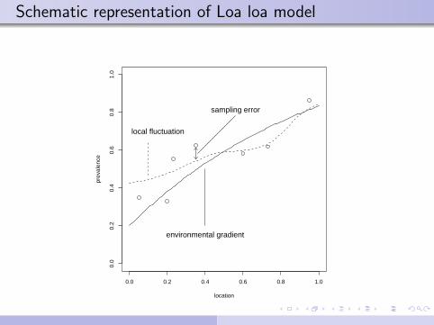
Schematic representation of Loa loa model

0.0 0.2 0.4 0.6 0.8 1.0

0.0

0.2

0.4

0.6

0.8

1.0

location

prev

alen

ce

environmental gradient

local fluctuation

sampling error

The Loa loa modelling strategy

use relationship between environmental variables andground-truth prevalence to construct preliminarypredictions via logistic regression

use local deviations from regression model to estimate smoothresidual spatial variation

model-based approach acknowledges uncertainty in predictions

“The answer to any prediction problem is a probability distribution”

Peter McCullagh

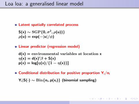
Loa loa: a generalised linear model

Latent spatially correlated process

S(x) ∼ SGP{0, σ2, ρ(u))}ρ(u) = exp(−|u|/φ)

Linear predictor (regression model)

d(x) = environmental variables at location xη(x) = d(x)′β + S(x)p(x) = log[η(x)/{1− η(x)}]

Conditional distribution for positive proportion Yi/ni

Yi|S(·) ∼ Bin{ni, p(xi)} (binomial sampling)

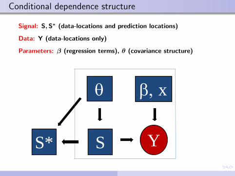
Conditional dependence structure

Signal: S, S∗ (data-locations and prediction locations)

Data: Y (data-locations only)

Parameters: β (regression terms), θ (covariance structure)

b, x q

Y S S*

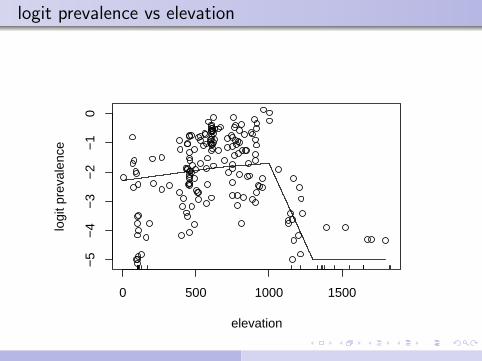
logit prevalence vs elevation

0 500 1000 1500

−5

−4

−3

−2

−1

0

elevation

logi

t pre

vale

nce

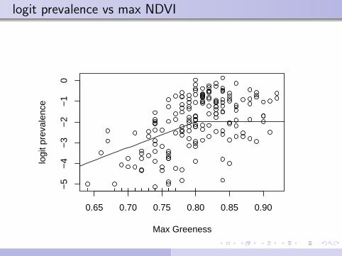
logit prevalence vs max NDVI

0.65 0.70 0.75 0.80 0.85 0.90

−5

−4

−3

−2

−1

0

Max Greeness

logi

t pre

vale

nce

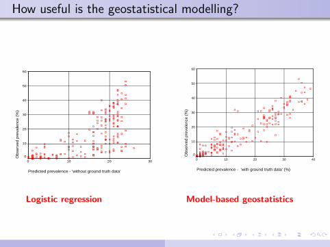
How useful is the geostatistical modelling?

Predicted prevalence - 'without ground truth data'

3020100

Ob

serv

ed

pre

vale

nce

(%

)

60

50

40

30

20

10

0

Predicted prevalence - 'with ground truth data' (%)

403020100

Obs

erve

d pr

eval

ence

(%

)

60

50

40

30

20

10

0

Logistic regression Model-based geostatistics

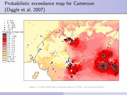
Probabilistic exceedance map for Cameroon(Diggle et al, 2007)

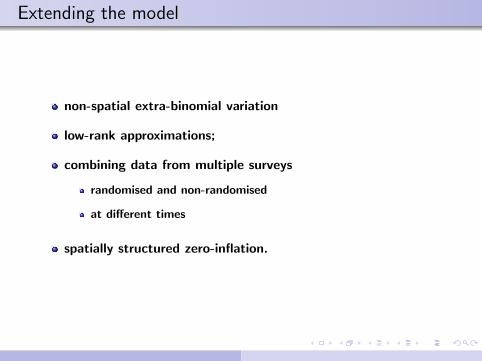
Extending the model

non-spatial extra-binomial variation

low-rank approximations;

combining data from multiple surveys

randomised and non-randomised

at different times

spatially structured zero-inflation.

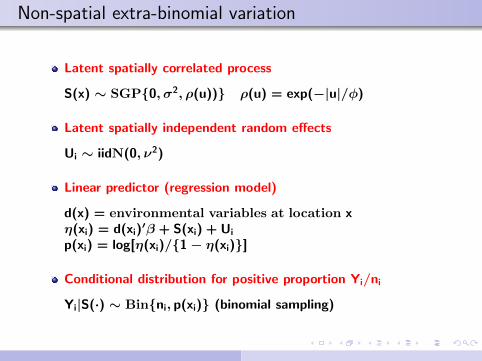
Non-spatial extra-binomial variation

Latent spatially correlated process

S(x) ∼ SGP{0, σ2, ρ(u))} ρ(u) = exp(−|u|/φ)

Latent spatially independent random effects

Ui ∼ iidN(0, ν2)

Linear predictor (regression model)

d(x) = environmental variables at location xη(xi) = d(xi)′β + S(xi) + Ui

p(xi) = log[η(xi)/{1− η(xi)}]

Conditional distribution for positive proportion Yi/ni

Yi|S(·) ∼ Bin{ni, p(xi)} (binomial sampling)

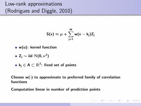
Low-rank approximations(Rodrigues and Diggle, 2010)

S(x) ≈ µ +M∑

j=1

w(x− kj)Zj

w(u): kernel function

Zj ∼ iid N(0, ν2)

kj ∈ A ⊂ IR2: fixed set of points

Choose w(·) to approximate to preferred family of correlationfunctions

Computation linear in number of prediction points

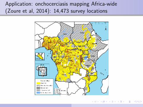
Application: onchocerciasis mapping Africa-wide(Zoure et al, 2014): 14,473 survey locations

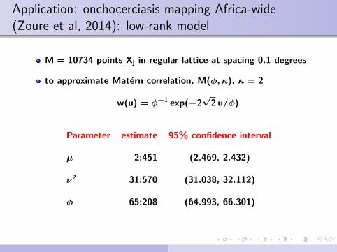
Application: onchocerciasis mapping Africa-wide(Zoure et al, 2014): low-rank model

M = 10734 points Xj in regular lattice at spacing 0.1 degrees

to approximate Matern correlation, M(φ, κ), κ = 2

w(u) = φ−1 exp(−2√

2 u/φ)

Parameter estimate 95% confidence interval

µ 2:451 (2.469, 2.432)

ν2 31:570 (31.038, 32.112)

φ 65:208 (64.993, 66.301)

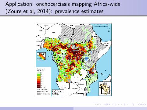
Application: onchocerciasis mapping Africa-wide(Zoure et al, 2014): prevalence estimates

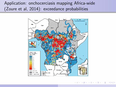
Application: onchocerciasis mapping Africa-wide(Zoure et al, 2014): exceedance probabilities

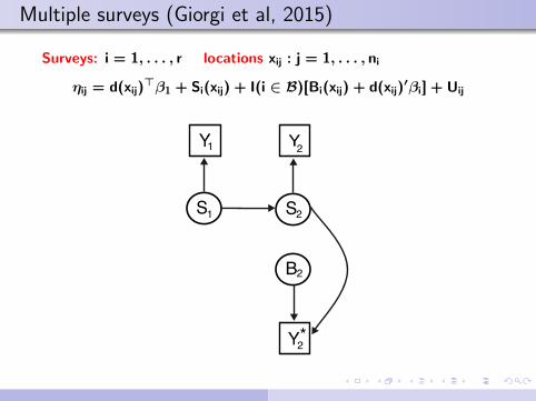
Multiple surveys (Giorgi et al, 2015)

Surveys: i = 1, . . . , r locations xij : j = 1, . . . , ni

ηij = d(xij)>β1 + Si(xij) + I(i ∈ B)[Bi(xij) + d(xij)

′βi] + Uij

1

S1

2*

B2

2

S2

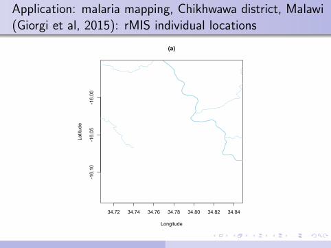
Application: malaria mapping, Chikhwawa district, Malawi(Giorgi et al, 2015): rMIS individual locations

34.72 34.74 34.76 34.78 34.80 34.82 34.84

-16.10

-16.05

-16.00

(a)

Longitude

Latitude

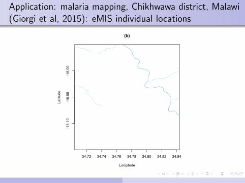
Application: malaria mapping, Chikhwawa district, Malawi(Giorgi et al, 2015): eMIS individual locations

34.72 34.74 34.76 34.78 34.80 34.82 34.84

-16.10

-16.05

-16.00

(b)

Longitude

Latitude

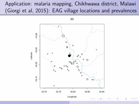
Application: malaria mapping, Chikhwawa district, Malawi(Giorgi et al, 2015): EAG village locations and prevalences

34.70 34.75 34.80 34.85 34.90

-16.10

-16.05

-16.00

-15.95

(c)

Longitude

Latitude

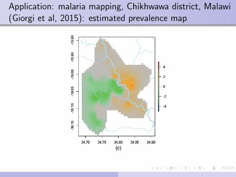
Application: malaria mapping, Chikhwawa district, Malawi(Giorgi et al, 2015): estimated prevalence map

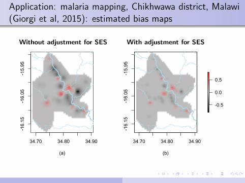
Application: malaria mapping, Chikhwawa district, Malawi(Giorgi et al, 2015): estimated bias maps

Without adjustment for SES With adjustment for SES

34.70 34.80 34.90

-16.15

-16.05

-15.95

(a)

34.70 34.80 34.90

-16.15

-16.05

-15.95

(b)

-0.5

0.0

0.5

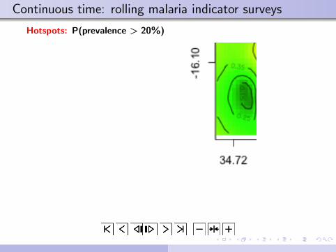
Continuous time: rolling malaria indicator surveys

Hotspots: P(prevalence > 20%)

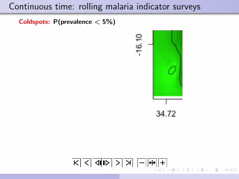
Continuous time: rolling malaria indicator surveys

Coldspots: P(prevalence < 5%)

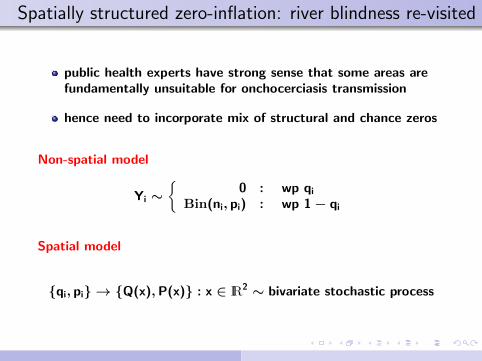
Spatially structured zero-inflation: river blindness re-visited

public health experts have strong sense that some areas arefundamentally unsuitable for onchocerciasis transmission

hence need to incorporate mix of structural and chance zeros

Non-spatial model

Yi ∼{

0 : wp qi

Bin(ni, pi) : wp 1− qi

Spatial model

{qi, pi} → {Q(x),P(x)} : x ∈ IR2 ∼ bivariate stochastic process

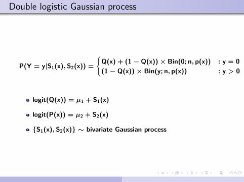
Double logistic Gaussian process

P(Y = y|S1(x), S2(x)) =

{Q(x) + (1− Q(x))× Bin(0; n, p(x)) : y = 0

(1− Q(x))× Bin(y; n, p(x)) : y > 0

logit(Q(x)) = µ1 + S1(x)

logit(P(x)) = µ2 + S2(x)

{S1(x), S2(x)} ∼ bivariate Gaussian process

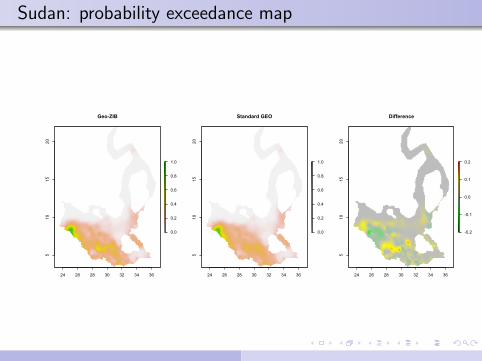
Sudan: probability exceedance map

24 26 28 30 32 34 36

510

1520

Geo-ZIB

0.0

0.2

0.4

0.6

0.8

1.0

24 26 28 30 32 34 36

510

1520

Standard GEO

0.0

0.2

0.4

0.6

0.8

1.0

24 26 28 30 32 34 36

510

1520

Difference

-0.2

-0.1

0.0

0.1

0.2

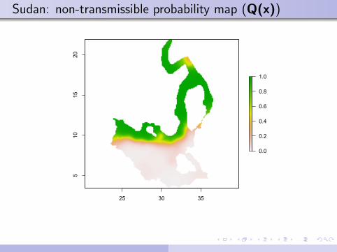
Sudan: non-transmissible probability map (Q(x))

25 30 35

510

1520

0.0

0.2

0.4

0.6

0.8

1.0

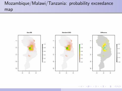
Mozambique/Malawi/Tanzania: probability exceedancemap

30 35 40

-25

-20

-15

-10

-5

Geo-ZIB

0.0

0.2

0.4

0.6

0.8

1.0

30 35 40

-25

-20

-15

-10

-5

Standard GEO

0.0

0.2

0.4

0.6

0.8

1.0

30 35 40

-25

-20

-15

-10

-5

Difference

-0.2

-0.1

0.0

0.1

0.2

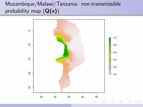
Mozambique/Malawi/Tanzania: non-transmissibleprobability map (Q(x))

25 30 35 40 45

-25

-20

-15

-10

-5

0.0

0.2

0.4

0.6

0.8

1.0

Implementation

Monte Carlo maximum likelihood

Plug-in prediction

R package PrevMap

Bayesian version?

Closing remarks

principled statistical methods

− make assumptions explicit

− deliver optimal estimation within the declared model

− make proper allowance for predictive uncertainty

but there is no such thing as a free lunch

“We buy information with assumptions”

C H Coombs

which is why statistics is at its most effective when conductedas a dialogue with substantive science

and this should guide the way we teach statistics ...especiallyto science students