Embed Size (px)
Citation preview

MODEL BASED DYNAMIC ANALYSIS
OF HUMAN SLEEP
ELECTROENCEPHALOGRAM
Thesis submitted for the degree of Doctor of
Philosophy at the University of Leicester
by
Yuehe Wang
Engineering Department
Leicester University
March 1997

UMI Number: U090574
All rights reserved
INFORMATION TO ALL USERS The quality of this reproduction is dependent upon the quality of the copy submitted.
In the unlikely event that the author did not send a complete manuscript and there are missing pages, these will be noted. Also, if material had to be removed,
a note will indicate the deletion.
Dissertation Publishing
UMI U090574Published by ProQuest LLC 2013. Copyright in the Dissertation held by the Author.
Microform Edition © ProQuest LLC.All rights reserved. This work is protected against
unauthorized copying under Title 17, United States Code.
ProQuest LLC 789 East Eisenhower Parkway
P.O. Box 1346 Ann Arbor, Ml 48106-1346

... O sleep, O gentle sleep,Nature’s soft nurse, how have I frighted thee, That thou no more wilt weight my eyelids down and sleep my senses in forgetfulness...
Shakespeare
{it has been considered that he suffered from insomnia)

MODEL BASED DYNAMIC ANALYSIS OF HUMAN SLEEP
ELECTROENCEPHALOGRAM
by
Yuehe Wang
Declaration of Originality
A thesis submitted in fulfilment of the requirements for the degree of Doctor of
Philosophy in the Department of Engineering, The University of Leicester, UK. All
work recorded in this thesis is original unless otherwise acknowledged in the text or
by references. No part of it has been submitted for any degree, either to the
University of Leicester or to any other university.
Yuehe Wang
March 1997

Acknowledgements
Firstly, I would like to express my thanks to Professor Barry Jones for his
kindness and his appreciation of my abilities (capabilities). Deepest thanks go to him
and to Dr. Chris D. Hanning (General Hospital, Leicester, UK.) for their
encouragement, advice and kindly help both academic and financial during my
Ph.D. studies in Leicester University. Without their support it would be impossible
for me to finish.
Particular thanks also go to Dr. John C. Fothergill and Dr. F.S. Schlindwein for
their extremely beneficial advice and supervision of my work.
I would like to express my gratitude to Dr.Chris Idzikowski (NCE Brainwaves,
N. Ireland), Dr. Stephen Roberts (Dept, of Engineering Science, Oxford University)
and James Pardey (Dept, of Engineering Science, Oxford University) for their
kindness in supplying the EEG data used and for their helpful advice. Many thanks
also go to Mrs. Jane Jones (NCE Brainwaves, N. Ireland) for staging sleep recording
used and teaching me the rudiments of EEG recording.
My research was made enjoyable by all members of the Biomedical Engineering
Group in the Dept, of Engineering at Leicester University. Thanks must go to Mr.
Yuhua Li, Dr. Paul Goodyer, Dr. Michael J. Pont, and Dr. Manho Kim, to name but
a few.
Thanks are also due to Dr. Zhonghe Wang, Dr. Lu Xiaoyun, Dr. Sun Wei and
Mr. Lou Zuhua for their valuable comments on my work and their enthusiastic
support.
Finally, very special thanks go to my wife Hao Wang and my parents who so
encouraged and supported me throughout the period of my stay in Leicester. I want
to thank Jeffrey, my son, for being bom.

Abstract
MODEL BASED DYNAMIC ANALYSIS OF
HUMAN SLEEP ELECTROENCEPHALOGRAM
Yuehe Wang Ph.D. thesisEngineering Department March 1997Leicester University
For sleep classification, automatic electroencephalogram (EEG) interpretation techniques are of interest because they are labour saving, in contrast to manual (visual) methods. More importantly, some automatic methods, which offer a less subjective approach, can provide additional information which it is not possible to obtain by manual analysis.
An extensive literature review has been undertaken to investigate the background of automatic EEG analysis techniques. Frequency domain and time domain methods are considered and their limitations are summarised. The weakness in the R & K rules for visual classification and from which most of the automatic systems borrow heavily are discussed.
A new technique — model based dynamic analysis — was developed in an attempt to classify the sleep EEG automatically. The technique comprises of two phases, these are the modelling of EEG signals and the analysis of the model’s coefficients using dynamic systems theory. Three techniques of modelling EEG signals are compared: the implementation of the non-linear prediction technique of Schaffer and Tidd (1990) based on chaos theory; Kalman filters and a recursive version of a radial basis function for modelling and forecasting the EEG signals during sleep. The Kalman filter approach produced good results and this approach was used in an attempt to classify the EEG automatically. For classifying the model’s (Kalman filter’s) coefficients, a new technique was developed by a state- space approach. A ‘state variable’ was defined based on the state changes of the EEG and was shown to be correlated with the depth of sleep. Furthermore it is shown that this technique may be useful for automatic sleep staging. Possible applications include automatic staging of sleep, detection of micro-arousals, anaesthesia monitoring, and monitoring the alertness of workers in sensitive or potentially dangerous environments.

vi
Contents
TABLE OF CONTENTS viLIST OF ABBREVIATIONS AND SYMBOLS ix
1. INTRODUCTION 1
1.1 Background 1
1.2 Signal acquisition 3
1.3 Sleep related signals 8
1.3.1 EEG signals 8
1.3.2 EMG signals 10
1.3.3 EOG signals 11
1.4 Sleep staging techniques 12
1.5 Sleep stage definitions 14
1.5.1 wakefulness 16
1.5.2 NREM sleep 16
1.5.3 REM sleep 18
2. REVIEW OF AUTOMATIC EEG ANALYSIS 25
2.1 Introduction 25
2.2 EEG interpretation 26
2.2.1 Interpretation in the frequency domain 26
2.2.2 Interpretation in the time domain 29
2.2.3 Fractal and deterministic chaos theory in EEG analysis 32
2.3 EEG feature classification 35
2.3.1 Techniques for automatic EEG feature classification 36

vii
2.3.2 EEG feature classification for sleep staging 38
2.4 Controversies over classification rules 39
3. DIFFERENTIAL TOPOLOGY 42
3 1 Basic topology 42
3.2 Quotient space and quotient topology 45
3.3 Tangent Bundles and Tangent Space 46
3.4 Vector fields and solutions 49
4. BACKGROUND THEORIES FOR MODELLING THE EEG 52
4.1 Introduction 52
4.2 Kalman filtering 54
4.2.1 Introduction 54
4.2.2 State-space representations 58
4.2.3 Kalman filter algorithm 61
4.3 Non-linear modelling techniques 70
4.3.1 Introduction 70
4.3.2 State space reconstruction (Method of delays) 73
4.3.3 Global prediction techniques 78
4.3.4 Local prediction techniques 79
4.3.5 Radial Basis Functions 81
5. MODELLING OF EEG 84
5.1 Introduction 84
5.2 EEG modelling using local prediction technique 86
5.3 EEG modelling using Kalman filter 91
5.3.1 Introduction 91
5.3.2 Model order 92
5.3.3 EEG modelling 96

viii
5.4 EEG modelling using Radial Basis Functions
- Adaptive non-linear modelling by a modified Kalman Filtering
approach 99
5.4.1 Introduction 99
5.4.2 Outline of the algorithm 100
5.4.3 EEG modelling 104
5.5 Performance comparison 109
6. A METHOD FOR CLASSIFYING THE COEFFICIENTS OF THE
MODEL 1216.1 Introduction 121
6.2 Embedding the model’s coefficients into their state space 124
6.3 Classifying the model’s coefficients 127
7. RESULTS 140
8. CONCLUSIONS AND FURTHER WORK 172
8.1 EEG interpretation 172
8.2 EEG feature classification 177
8.3 Discussion 178
8.4 Further work 180
REFERENCE
APPENDICES
A. Akaike’s Final Prediction Error criterion
B. Details of the EEG signals used

LIST OF ABBREVIATIONS AND SYMBOLS
ANFIS Adaptive-Network-based Fuzzy Inference System
APs Action potentials
AR Autoregressive model
ARMA Autoregressive moving-average model
ARMAX Autoregresive moving-average model with exogenous
inputs
ARX Autoregressive model with exogenous input
ED Embedding dimension
EEG Electroencephalogram
EKF Extended Kalman filter
EMG Electromyogram
EOG Electrooculogram
FFT F ast F ourier transform
FIR Finite impulse response model
FPE Akaike’s Final Prediction Error

HR
MA
ME
MT
MU
MUAP
NLF
NPE
NREM
PA
PSPs
R & K rules (criteria)
RBF
REM
Infinite impulse response model
Moving-average model
Burg's maximum entropy
Movement time
Motor units
Motor unit action potential
A package of Non-linear Forecasting For Dynamical
Systems
Normalized prediction error
Non-rapid eye movement sleep
Atlas points or points used for embedding
Post-synaptic potentials
Rechtschaffen and Kales scoring system for sleep
Stages of human subjects
Radial Basis Functions
Rapid eye movement sleep

Chapter 1
INTRODUCTION
This chapter contains some historical and technical vignettes, as a modicum of
background knowledge which is necessary in order to show how a small plant has
grown into a remarkable tree.
1.1 Background
The nature of sleep has been a topic of constant interest since antiquity (over
2000 years), but systematic research on sleep and sleep mechanisms began only in
the 19th century and it is only in recent years that the true importance of sleep
studies both in clinical and scientific applications has been recognised.
In 1929, Hans Berger first recorded the electrical activity, termed the
electroencephalogram (EEG), of the human brain. Since then, the application of
EEG in characterizing different levels of sleep by Loomis paved the way to the

Chapter 1. INTRODUCTION 2
discovery by Aserinsky and Kleitman that sleep consisted of two distinct phases
rather than a single one which merely varied along a continuum in depth. In Loomis’
time, EEG patterns were classified from wakefulness to sleep into five stages, (A,
B l, B2, C, D, and E). This classification was widely adopted, until some years later
(in 1953), Aserinsky and Kleitman discovered rapid eye movement (REM) sleep.
Dement and Kleitman then (in 1953) proposed a classification system, in which
REM was differentiated from non-rapid eye movement (NREM) sleep. This system
was modified by Rechtschaffen and Kales in 1968 (R & K rules) and has been the
most widely used since then.
Traditionally, the most important aspect of sleep analysis is sleep staging by
visual assessment of the EEG, electrooculogram (EOG) and electromyogram (EMG)
by trained observers using a set of standardised rules (i.e. R & K rules).
Computerised analysis of sleep recordings was first tried in 1968 (Lacroix, 1984).
Since then, a number of automated systems have been developed for EEG analysis,
but few of them have been designed for routine sleep staging in a clinical
environment (Stanus, 1987). Automatic sleep staging and automatic EEG
interpretation techniques are of interest not only because they are labour saving, but
also because they can be made consistent and quantitative in contrast to manual
methods. More importantly, automatic methods may provide additional information
which is not obtainable by manual analysis

Chapter 1. INTRODUCTION 3
Although a great deal of work has been done on sleep since the 1930s, there is
still much that we do not know and there are many controversies that have not been
resolved.
1.2 Signal acquisition
In order to identify and classify sleep, it is necessary to monitor simultaneously
the electrical activity of three systems: the brain (by means of EEG), the movement
of the eyes (by means of EOG), and the muscles tone (by means of EMG). The
recording of the EEG is a very important technique in studies on sleep. Much of our
current knowledge concerning sleep has been made possible by the use of EEG
recording techniques. The EEG, EMG and EOG have provided an apparently
"objective" basis for the study of sleep and sleep related phenomena.
There are two techniques that can be used for EEG aquisition, invasive or
non-invasive recording. The most widely used is that non-invasive method from the
scalp by means of surface electrodes. Obviously, the advantage of non-invasive
procedures in the sleep environment is that it does not cause significant patient
discomfort, so that there is little risk of disrupting the sleep process.
As the activity recorded differs from one region of the scalp to another, in a full
EEG recording session, up to 20 channels are recorded simultaneously with the
electrodes distributed widely over the head. In contrast, sleep EEG recordings use 1

Chapter 1. INTRODUCTION 4
to 4 channels and are recorded in parallel with EOG and/or EMG recordings. EEG
signals may be measured in three ways: (i) from single electrodes each with
reference to a common electrode (usually on the mastoid or preauricular point); (ii)
between pairs of electrodes; or (iii) from single electrodes with respect to the
average of all the other electrodes.
The first step for the electrode attachment is the measurement of electrode
positions according to the so called international 10-20 system of electrode
placement. Figure 1.1 illustrates the 10-20 placement system and the reliable
recording of EEG relies on accurate measurement of the skull according to this
system.
After measurements are made, the skin or superficial dermis, where the
electrodes will be placed, needs to be degreased and cleansed thoroughly by brisk
rubbing with gauze or cotton wool on which acetone or now, more commonly, skin
prep has embedded, (skin prep contains some impedance reducing electrolyte
material.) This is generally sufficient to ensure adequate conduction when the
electrode is applied. EEG electrodes should be non-polarisable and of the
silver/silver chloride type (or gold type) attached to the scalp with collodion. The
electrolyte under the electrode should be scooped into the electrode before the
electrode is glued in place. While by using Montreal Neurological Institute type of
electrode, which has a hole in the back, the electrolyte can be added after the
electrode is glued tightly on the head. Moreover this electrode is very helpful for
long time, such as over night sleep, recording (10 - 12 hours), as it has a hole in the

Chapter 1. INTRODUCTION 5
back of the electrode through which further electrolyte paste may be added during
the recording. Electrode impedance must be carefully checked before recording. It
should be less than 5 kilohms.
N asion '
P re a u r ic u la rP o in t
In io n
Figure 1.1 Schematic diagram showing measurements for the
international 10-20 electrode placement system.
For routine recording of EOG, the R and K manual recommends referential
recordings from each outer canthus to the ipsilateral ear (or side of neck). The
electrodes should be offset from horizontal, one slightly above and one slightly
below the horizontal plane. These derivations have the advantage of showing
horizontal and vertical eye movements as out-of-phase potentials in the two
channels. However, they have the disadvantage of containing much EEG artifact in

Chapter 1. INTRODUCTION 6
the leads, especially in slow wave sleep when the EEG reaches maximum amplitude.
The eye movement electrodes should be non-polarisable and of stick-on type.
Regular EEG electrodes could be used. The skin need to be cleansed as in
preparation for EEG leads. It is recommended that they are kept in place by
microporous adhesive tape or sticky discs which retains its adhesion well over long
recording. As the upper limit of the EOG frequency band is much lower than that of
EEG, an EEG recording channel can be used without further modification.
The EMG is taken as the potential between two electrodes, one on each side of
the neck beneath the chin over the mylohyoid and digastric muscles. Stick-on
silver/silver chloride electrodes may be used, and regular EEG electrodes could be
used. As in the case of EEG and EOG recording, the skin is thoroughly cleansed
before applying the electrodes. General requirement of impedance for each electrode
need to be less than 5 kilohms. Sticky discs and flexible adhesive tape are
recommended to place the electrodes firmly on the skin. The electrodes are
connected by bipolar linkage to a single channel. It is often adequate for indicating
the presence of muscular activity by using an EEG channel with the highest possible
frequency response (usually 70 - 100 Hz) for recording of EMG activity in most
instances.
In sleep studies, the most commonly used placement of the electrodes for the
EEG, EMG, and EOG recording is shown in Figure 1.2, by which the upper drawing
represents recommendations for placement of electrodes (El, E2, A1 and A2) for

Chapter 1. INTRODUCTION 7
recording eye movements (EOG) and electrodes for recording EMG; lower drawing
shows recommendations for placement of C3/A2, and/or C4/A1 electrodes for
recording EEG. In some laboratories an occipital EEG (usually 01 /A2 or 02/A1) is
record routinely as an adjunct to the central EEG. It is particularly useful for
assessing sleep onset or arousals during sleep.
LEFT EYE - A1
RIGHT EYE - A1
EMG
C4 - A1
Figure 1.2 Electrode placement in sleep research. (From
Rechtschaffen and Kales, 1968)

Chapter 1. INTRODUCTION 8
1.3 Sleep related signals
1.3.1 EEG signals
EEG analysis is concerned with the study of a small, constantly changing
electrical potentials form the brain which can be collected from scalp electrode. The
electrode, with about 100 mm2 in area, converges the averaged electrical activity
from a substantial volume of underlying cortex through the thickness of skull and
meninges. It was originally thought that EEG waves might be made up of summated
action potentials, but because their short duration ( 1 - 2 ms) tend to overlap much
less than do Post-synaptic potentials (PSPs). PSPs are of electrical changes in the
post-synaptic membrane with lower amplitude than the action potential and last
longer, 10 - 250 ms. Enough evidence, exists to state that the EEG on the scalp is
mainly composed by synchronously occurring PSPs, (for example, the research of
simultaneous recordings o f the activity of individual neurones and of the overlying
EEG achieved by O.D. Creutzfeldt, et al. 1966). It has been estimated that
synchronous PSPs in only 1% of cortical neurones would be sufficient to account for
the signals normally seen in the EEG.
The frequency range of the scalp EEG has a fuzzy lower and upper limit. The
major power distributes in the range of 0.5 to 60 Hz in which most EEG studies for
clinical and research purposes are carried out. This may reflect the limitations of the
recording systems rather than the actual range of activity present. There is for

Chapter 1. INTRODUCTION 9
instance evidence that EEG contains information at over 200 Hz. However, the ultra-
slow and ultra-fast frequency components play no significant role in the clinical
analysis. By convention, and partly for historical reasons, the frequency range is
subdivided into four frequency bands which are:
Delta (8) — below 4 Hz;
Theta (0) — not less than 4 but less than 8 Hz;
Alpha (a) — 8 to 13 Hz inclusive;
Beta (p) — More than 13 Hz.
Amplitudes of the scalp EEG range from 10 to lOOpV rarely exceeding 150 pV in a
normal waking subject. EEG amplitudes vary with many factors, such as age,
electrode placement and skull morphology, therefore the precise determination of the
voltage of each wave is unnecessary and should be discouraged.
The EEG signal, which reflects the general functional state of the brain, has
become a standard measurement made in clinical neurophysiology. In sleep studies,
EEG is the core measurement in polysomnography. The four stages of NREM sleep
are distinguished from one another principally along this signal.
The EEG changes continually in a random manner, and in association with
wakefulness and sleep cycle. It also changes gradually over the lifetime of the
individual and shows marked differences between one person and another.

Chapter 1. INTRODUCTION 10
1.3.1 EMG signals
EMG is the study of electrical activity in the muscles. With electrodes placed on
the skin surface, the signal recorded when a muscle contracts is known as the surface
EMG. EMG is one of the largest and most easily measured bioelectrical signals.
When quantified in some way it is very reliable indicator of whether a muscle is
active.
Muscle fibres are organised into functional units within a muscle, which are
called motor units (MU). The fibres belonging to one MU are spread over a certain
area of the muscle cross-section, and are thus intermingled with fibres from several
other MUs. A MU consisting of several muscle fibres is innervated by a single
motor neuron. Roughly at the midpoint along the length of each muscle fibre is an
endplate, where action potentials (APs) are generated after synaptic transmission
from the motor nerve. The muscle fibres as well as the nerves obey the “all-or-
nothing” law, i.e. they have two states: inactive and excited. When the motor neuron
is activated, all muscle fibres in the MU respond, producing a motor unit action
potential (MUAP) which is the temporal and spatial summation of the APs of all
muscle fibres in the MU. At low contraction levels few motor units are active. With
increasing contraction strength, the firing rate of these motor units increases and
new, larger motor units are recruited. Even at moderate contraction levels single
MUAPs tend to overlap, producing a random like signal, the interference (quite
complex) EMG.

Chapter 1. INTRODUCTION 11
The EMG signal is composed of a mixture of different frequency components,
with most of the signal energy falling within the 10 to 1000 Hz range.
EMG recording is essential for the study of certain types of muscle activity
during sleep. In the standard polysomnographic recording, the EMG is used as a
criterion for staging REM sleep. The level of tonic EMG is normally absent in REM
sleep. In addition of NREM sleep, the level of EMG usually decreases from
wakefulness through stages 1, 2, 3 and 4.
1.3.1 EOG signals
The EOG records the electrical potential generated within the eye, and is made
simply to document the presence or absence of eye movements.
The EOG recordings are based on the small electrical potential difference, often
over 200 pV, from the front to the back of the eye. The cornea is positively-charged
with respect to the negatively-charged retina. Therefore, the eye ball acts as a
potential field within a volume conductor in the head. Because of this essentially
constant potential difference between the retina and the cornea, movement of the
eyes can be measured from electrodes placed beside the eyes. An electrode nearest
the cornea will register a positive potential; an electrode nearest the retina will
register a negative potential. As the eye moves, the positions of the cornea and retina
change relative to a fixed position of the electrode, and a potential change will
registered by the electrode.

Chapter 1. INTRODUCTION 12
The EOG has an amplitude of about 20 pV per degree of rotation of the eyeball,
and frequency response up to about 30 Hz is adequate for the recording most of the
rapid eye movements
In sleep research, for the recognition of sleep stages, eye movement recording is
necessary for sleep staging and it is required by the R and K criteria. That is the
rolling eye movements of stage 1 and the rapid eye movement of stage REM. Eye
movement recording by means of EOG is also useful in EEG recording for the
identification of eye movement artifacts.
1.4 Sleep staging techniques
Conventionally, sleep stage is visually assessed from a paper record by an
expert human observer. Three parameters (EEG, EOG and EMG) to assess sleep
according to internationally standardized criteria (R & K. rules) are needed, and
EEG is the core measurement among them. This classification of different sleep
stages is based on patterns of EEG waveforms (i.e., delta waves, K-complexes, theta,
alpha, beta waves, and sleep spindles in the EEG channels), combined with eye
movement in the EOG channel, and the bursts of muscle activity in the EMG
channel when available.
The R. & K. rules provide detailed guidelines and criteria for staging normal
human sleep. When staging a sleep recording, it is necessary and convenient to
Chapter 1. INTRODUCTION 13
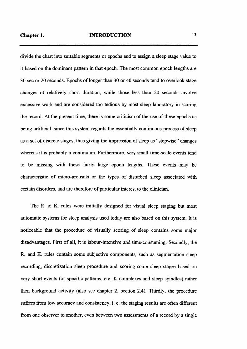
divide the chart into suitable segments or epochs and to assign a sleep stage value to
it based on the dominant pattern in that epoch. The most common epoch lengths are
30 sec or 20 seconds. Epochs of longer than 30 or 40 seconds tend to overlook stage
changes of relatively short duration, while those less than 20 seconds involve
excessive work and are considered too tedious by most sleep laboratory in scoring
the record. At the present time, there is some criticism of the use of these epochs as
being artificial, since this system regards the essentially continuous process of sleep
as a set of discrete stages, thus giving the impression of sleep as “stepwise” changes
whereas it is probably a continuum. Furthermore, very small time-scale events tend
to be missing with these fairly large epoch lengths. These events may be
characteristic of micro-arousals or the types of disturbed sleep associated with
certain disorders, and are therefore of particular interest to the clinician.
The R. & K. rules were initially designed for visual sleep staging but most
automatic systems for sleep analysis used today are also based on this system. It is
noticeable that the procedure of visually scoring of sleep contains some major
disadvantages. First of all, it is labour-intensive and time-consuming. Secondly, the
R. and K. rules contain some subjective components, such as segmentation sleep
recording, discretization sleep procedure and scoring some sleep stages based on
very short events (or specific patterns, e.g. K complexes and sleep spindles) rather
then background activity (also see chapter 2, section 2.4). Thirdly, the procedure
suffers from low accuracy and consistency, i. e. the staging results are often different
from one observer to another, even between two assessments of a record by a single

Chapter 1. INTRODUCTION 14
scorer. Therefore, an alternative, rapid and objective assessment of sleep recording is
desirable in a clinical environment.
Automatic sleep staging and/or automatic EEG analysis are becoming important
tools in this field because they are labour saving and can be made consistent and
quantitative in contrast to manual methods. More importantly, automatic methods
may provide additional information which are not obtainable by manual analysis,
such as the detection of brief arousals. Although a number of automated systems
have been developed for EEG analysis during the last 20 years, few of them have
been designed for routine sleep staging in a clinical environment (Stanus, 1987).
The techniques used in visual sleep staging are relatively unchanged from
Rechtschaffen and Kales time (1968) and an overall review can be found in papers
of Hasan (1983), Binnie (1982), and Cox Jr. (1972).
1.5 Sleep stage definitions
Traditionally the most important aspect of sleep analysis is sleep staging. Based
on a collection of physiological parameters (i.e. EEG, EOG, and EMG), two separate
states have been defined within sleep. These are the states of non-rapid eye
movement (NREM) and rapid eye movement (REM), NREM and REM exist
virtually in all mammals and birds.
NREM sleep is conventionally subdivided into four stages (i.e., stage 1, 2, 3 and
4), which are mainly defined along one measure of EEG. The EEG pattern in NREM

Chapter 1. INTRODUCTION 15
sleep is commonly described as synchronous, with such characteristic waveforms as
sleep spindles, K complexes, and high-voltage slow waves. REM sleep generally is
not divided into stages, and it is, by contrast, defined by episodic bursts of rapid eye
movements, muscle atonia, and EEG activation. NREM sleep and REM sleep
continue to alternate through the night in cyclic fashion with a period of about 90 to
110 minutes. The normal adult human enters sleep through NREM sleep (begins
with sleep stage 1), and REM sleep does not occur until about 80 minutes or later.
REM sleep episodes generally become longer across the night. Sleep stages 3 and 4
occupy less time in the second cycle and may disappear altogether from later cycles,
as the sleep stage 2 expands to occupy the NREM portion of the cycle.
The hypnogram, see figure 1.3, is a plot of sleep stage against time. Movement
time (MT) and wakefulness as additional stages may be added into the hypnogram.
According to R. and K. rules, large body movements are associated with high
amplitude EMG activity which commonly also involves EEG and EOG channels.
When the EEG and EOG are obscured by such muscle tension and/or amplifier
blocking artefacts for more than half of an epoch it is impossible to stage it and the
epoch is scored as movement time (MT). For a normal young adult the hypnogram
typically takes the form shown in figure 1.3.
In summary, sleep stages may be defined as follows:

Chapter 1. INTRODUCTION 16
1.5.1 Wakefulness
An overnight recording usually contains a period of wakefulness before sleep
onset in which the individual normally is in a relaxed state with eyes closed. During
this relaxed wakefulness, the EEG is composed predominantly of sinusoidal alpha
activity (8 -13 Hz inclusive) intermixed with lower amplitude irregular beta waves
(more than 13 Hz). Alpha activity is the most important feature though this may be
suppressed by attention and anxiety or blocked if the subject is looking about.
Muscle tone is generally high, and eye movements may be present, such as eyelid
blinks or slow rolling movements. As the subject becomes more drowsy, alpha
activity decreases with accompanying relatively slow activity.
1.5.2 NREM sleep
The NREM state is often called “quiet sleep” because of the slow, regular
breathing, the general absence of body movement, and the slow, regular brain
activity shown in the EEG.
Sleep stage 1
Stage 1 is characterized by the great decrease of alpha activity (less than 50% of
the record), some increase in beta which is a low-amplitude mixed-ffequency signal
and the slower theta ( 4 - 7 Hz) activity. In the EOG channel slow lateral eye
movements may appear. As the subject progresses toward stage 2, the slower

Chapter 1. INTRODUCTION 17
activity predominates and vertex sharp waves may appear with an increase in slow
components especially in younger subjects.
Stage 1 in the normal young adult occupies approximately 2 - 5% of total night
time sleep and often occurs as a transition from wakefulness or body movements
during sleep to other sleep stages.
Sleep stage 2
This is composed of largely a theta and beta background with some low-
amplitude delta components comprising less than 20% of the record, and is
characterized by the appearance of two types of intermittent events; the spindles and
K-complexes. Spindles are brief bursts of rhythmic 12-14 Hz waves, lasting at least
0.5 second. K-complexes are composed of a high-amplitude negative wave followed
by a positive wave. Sometimes brief bursts of low-amplitude 12-14 Hz activity may
be superimposed on the K-complex. It should be noted that in addition to its
spontaneous appearance during stage 2 sleep, the K-complex can occur at other
times in the sleeping person in response to auditory stimuli. The EMG shows some
tonic activity but this is less than in stage 1 and significantly less than in the waking
stage.
Stage 2 occupies the greatest amount of total sleep time in the normal young
adult about 45 - 55%.

Chapter 1. INTRODUCTION 18
Sleep stage 3
This stage is characterized by the appearance in between 20 -50 % of the epoch
of slow wave activity (at less than 2 Hz), which are high amplitude (at least 75 pV
from peak to peak). Collectively, stage 3 and stage 4 are often referred to as slow-
wave sleep.
Sleep stage 4
In stage 4 slow wave activity makes up more than 50% of the epoch. Sleep
spindles may or may not be present during stage 3 or 4.
Stage 3 normally occupies about 3 - 8% and stage 4 occupies 10 - 15% of
normal over-night sleep in the young adult.
1.5.3 REM sleep
REM sleep, which has been called “active sleep” is an entirely different sleep.
A REM sleep period is characterised by three main features. The first is the
presence of conjugate rapid eye movements. The second that is during REM sleep
the EEG returns to a mixed frequency pattern with medium amplitude, and similar to
stage 1 except that vertex sharp waves are not prominent. In contrast to stage 2, there
are no sleep spindles or K-complexes in REM sleep. The third is that the EMG drops
to very low amplitude, indicating the decrease in tone of the submental muscles.

Chapter 1. INTRODUCTION 19
Under regular EEG laboratory conditions, the observation of REM sleep
requires a long waiting period, since the first phase of REM does not appear prior to
60 to 90 minutes after sleep onset in a normal night time sleep.
Figure 1.4 shows the typical EEG patterns, eye movement in right and left
EOG, and chin EMG patterns for different sleep stages and wakefulness.

Chapter 1. INTRODUCTION 20
Wake
MT
REM
10050 150 2500 200 300 350Time (Minutes)
Figure 1.3 The hypnogram for a normal young adult.
MT = Movement Time.
REM = Rapid eye movement.

Chapter 1. INTRODUCTION 21
L. EOG
R. EOG
EMG
1. Sec.
I = 50 p.V WAKE
(a)L. EOG
- - - - - - - - 1-— | —“ * y — * " ' j
R. EOG
EMG , I
^ V V v ^ v 1
1 Sec.
= 50HV STAGE 1
(b)
Figure 1.4. Stages of sleep as recorded on the EOG, EMG and EEG. (a)
Wakefulness; (b) sleep stage 1. (Stages 2, 3 ,4 and REM are shown on the next
pages.)

Chapter 1. INTRODUCTION 22
L EOG
R. EOG
EM G
EEG
= 50 HV STAGE 21 Sec.
(c)
L. EOG
R. EOG
1 Sec.
I = 50 HV STAGE 3
(d)Figure 1.4 continue. Stages of sleep as recorded on the EOG, EMG and EEG. (c)
Sleep stage 2; (d) sleep stage 3. (Stage 4 and REM are shown on the next page.)

Chapter 1. INTRODUCTION 23
R. EOG
EEG
MJ = 50 p.V
1 Sec.
STAGE 4
(e)
L. EOG
R EOG
EMG
EEG *
W VV'WM
J = 50 nV1 Sec.
STAGEREM
(f)
Figure 1.4 continue. Stages of sleep as recorded on the EOG, EMG and
EEG. (e) Sleep stage 4; (f) REM sleep. Note the high EMG and

Chapter 1. INTRODUCTION 24
eye movements during wakefulness, Sleep stage 2 is
characterized by sleep spindles and K-complexes as showed
underline. The EEG is similar during stage 1 and stage REM,
but the EMG is high and REMs are absent in stage 1. Stage 3
and 4 are characterized by slowing of frequency and increase in
amplitude of the EEG. (From Mendelson W.B. et al., 1977.)

Chapter 2
REVIEW OF AUTOMATIC EEG
ANALYSIS
2.1 Introduction
Most of the automatic procedures for sleep EEG staging include feature
extraction from the EEG followed by the use of these features for classification of
the EEG into various stages (EEG classification).
This chapter will present the background and traditional methods of EEG
analysis based on its interpretation and classification in the context of sleep studies.
Frequency domain and time domain methods are considered and their limitations are
summarised briefly. The novel techniques of fractal and deterministic chaos theory
used for EEG analysis are included. Consequently, the EEG feature classification
techniques are reviewed. Finally, the weaknesses in the R & K criteria for visual
classification and from which most of the automatic systems borrow heavily will be

Chapter 2 REVIEW OF AUTOMATIC EEG ANALYSIS 26
discussed. No attempt has been made in this chapter to provide a comprehensive list
of references, but a sufficiently representative sample of the recent literature is
included.
2.2 EEG interpretation
Many methods of EEG interpretation have been developed in the last few
decades. These methods can be broadly grouped into the two main categories of
frequency domain and time domain methods. Frequency domain analysis is based on
the assumption that the EEG can be interpreted as a collection of periodical signals,
whilst in time domain analysis the consecutive EEG waves are treated as a series of
aperiodic phenomena. In addition, time domain methods normally tend to mimic the
non-automatic interpretation process of a human operator.
2.2.1 Interpretation in the frequency domain
The most used frequency domain method in EEG study is spectral analysis,
which is effective in characterizing dominant quasi-periodic rhythms (Lim A. J. and
Winters W. E., 1980). This method is mainly used for the analysis of background
electrical activity and spectra are computed from fixed-length signal segments
(epochs) of about 30s duration. This yields good results when the background
activity is abnormal but the short time structure of the EEG is lost in this approach
(Bodenstein, 1977). Spectral analysis based on parametric (autoregressive

Chapter 2 REVIEW OF AUTOMATIC EEG ANALYSIS 27
modelling) or non-parametric methods (e.g. fast Fourier transform) have been major
tools for the representation of the EEG signal segments.
In the parametric method based on linear predictive filtering there are several
approaches using autoregressive moving average (ARMA) and autoregressive (AR)
algorithms (Sanderson, 1980; Bodenstein, 1977; Balocchi, 1987; Lopes da Silva,
1981). An evaluation of these simple algorithms was carried out by W. D. Smith
(1986). The AR method, which was reportedly able to provide high resolution
spectral estimates from short time intervals, has already been applied to EEG
spectral estimation, EEG simulation, transient detection, and the detection of
segment boundaries in several ways (Bodenstein, 1977). The use of a Kalman filter
algorithm (which can be treated as an adaptive AR model) for EEG analysis was
originally introduced by Bohlin (1971) and has been employed by several
researchers (Roberts, 1991; Skagen, 1988; Bartoli and Cerutti, 1982). Jansen (Jansen
et al., 1981) found that the Kalman filter coefficients gave a qualitatively better
description of the spectral properties of the EEG over a longer period of time than
other non-adaptive AR models. However, when the EEG signal is highly non-
stationary, such as in the case of the occurrence of a large artifact, the artifact will
influence the filter coefficients for several seconds thereafter and thus produce
inaccurate spectral estimates for the current epoch. The Burg's maximum entropy
(ME) algorithm avoids this problem by using data only in the interval being
analysed. In Jansen's studies a comparison of spectral analyses from a Kalman filter,
a stationary AR model (derived from the Yule-Walker equations) and Burg's method

Chapter 2 REVIEW OF AUTOMATIC EEG ANALYSIS 28
was described. Because the Yule-Walker approach sometimes results in unstable
models Jansen et al suggested that it should not be used.
Of the non-parametric methods, the Fourier transform, which may have first
been used in EEG analysis by Dietsch (1932), has been most widely applied
(Scheuler, 1990; Pigeau, 1981; Jervis, 1989; Lacroix and Hanus, 1984; Dumermuth,
1983). It has provided good results and has become more easily implemented with
the introduction of the fast Fourier transform (FFT). There are, however, some well-
known drawbacks related to the Fourier analysis of EEG signals, such as the
enhancement of low-frequency components connected with the shape of the epoch
window (Daskalova, 1988). There seems to be a tendency for the use of the FFT to
be superseded to some extent by AR techniques in recent years, especially as their
computation time (about three times that of a comparable FFT) is no longer a
problem with fast modem computers.
Other approaches to non-parametric methods include: the Walsh transformation
(Li, 1990), power spectral density (Torbjom, 1986; Saltzberg, 1985), individual
frequency band analysis (Laurian, 1984; Barcaro, 1983; Scheuler, 1988), coherence
analysis (Sterman, 1977), and EEG variance (Hiroyoshi, 1991). Hao (1992) used
complex demodulation (the Hilbert transform), which enables the amplitude and
phase of particular frequency components to be described as functions of time so
that the instantaneous frequencies of sleep spindles in the EEG may be estimated.
Several of the methods for detection of sleep spindles are in the frequency domain

Chapter 2 REVIEW OF AUTOMATIC EEG ANALYSIS 29
(Pivik, 1982; Fish, 1988). Recently, Sauter (1991) used an asymptotic local
approach for the detection of spindles together with an AR model.
The analysis methods in the frequency domain have proved very useful. Most
EEG spectra exhibit a distinctive structure in which peaks and valleys can be clearly
distinguished and it is the peaks (corresponding to ’’rhythms") to which most
attention has been devoted.
2.2.2 Interpretation in the time domain
Although spectral analysis of EEG has provided a considerable amount of
information, some of the significant EEG patterns are aperiodic, e.g. K-complexes
and spike waves. The identification of these aperiodic events is critical to both
diagnostic EEG and to sleep stage EEG. To detect these aperiodic waveforms
different data-processing techniques (many in the time domain) may be employed.
The method of visual interpretation of the EEG is considered as a time domain
classification in which the electroencephalographer sees the paper record as a series
of waves of varying duration ("period", "interval", or "wave duration"). As already
mentioned, many methods of automatic EEG interpretation in the time domain
mimic the visual process. Thus, there is a family of techniques of "period analysis".
This family has two groups: the first one defines individual waves by the points at
which the signal passes through a base-line or near zero threshold and is known as

Chapter 2 REVIEW OF AUTOMATIC EEG ANALYSIS 30
the level-crossing technique; the second defines the waves by peaks and troughs, the
so-called peak detection technique.
One of the first methods of period analysis was proposed by Cohn (1963). He
used a level-crossing technique to obtain a histogram of the number of pulses with
respect to inter-pulse interval. The other approaches at that time were by Legewie
(1969, zero-crossing technique) and Leader (1967, peak detection method). In 1980,
Lim combined zero-crossing and peak detection algorithms for sleep stage analysis.
Methods based on level-crossing detection tend to favour slow waves, while
those based on peak detection tend to favour fast waves (Lim, 1980; Kuwahara,
1988). This family of techniques suffers from problems associated with the
uncertainty in base line position and its fluctuations; these affect the accuracy of the
period measurements. Sometimes a high-pass filter or a complicated method of
finding the waveform midpoints or inflection points is used. Leader (1967) tried to
overcome the problem by the use of waveform midpoint detection. Daskalova
(1988,) used the alternative technique of finding the minima and maxima of
successive waves, which does not depend on the base line position. The method of
period analysis has been further improved by taking into account both the period and
the peak amplitudes of the EEG waves by Carrie (1971), Dascalov (1974), and
Palem (1982).
A novel approach was described by Hjorth (1970), who proposed a description
of the EEG in terms of three normalized slope descriptors: “activity”, “mobility” and
Chapter 2 REVIEW OF AUTOMATIC EEG ANALYSIS 31
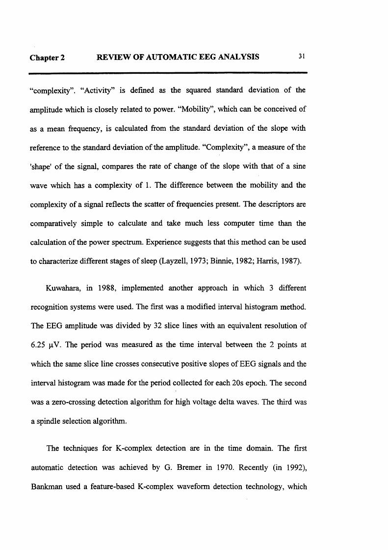
“complexity”. “Activity” is defined as the squared standard deviation of the
amplitude which is closely related to power. “Mobility”, which can be conceived of
as a mean frequency, is calculated from the standard deviation of the slope with
reference to the standard deviation of the amplitude. “Complexity”, a measure of the
'shape' of the signal, compares the rate of change of the slope with that of a sine
wave which has a complexity of 1. The difference between the mobility and the
complexity of a signal reflects the scatter of frequencies present. The descriptors are
comparatively simple to calculate and take much less computer time than the
calculation of the power spectrum. Experience suggests that this method can be used
to characterize different stages of sleep (Layzell, 1973; Binnie, 1982; Harris, 1987).
Kuwahara, in 1988, implemented another approach in which 3 different
recognition systems were used. The first was a modified interval histogram method.
The EEG amplitude was divided by 32 slice lines with an equivalent resolution of
6.25 pV. The period was measured as the time interval between the 2 points at
which the same slice line crosses consecutive positive slopes of EEG signals and the
interval histogram was made for the period collected for each 20s epoch. The second
was a zero-crossing detection algorithm for high voltage delta waves. The third was
a spindle selection algorithm.
The techniques for K-complex detection are in the time domain. The first
automatic detection was achieved by G. Bremer in 1970. Recently (in 1992),
Bankman used a feature-based K-complex waveform detection technology, which

Chapter 2 REVIEW OF AUTOMATIC EEG ANALYSIS 32
involved neural networks and provided good agreement with visual K-complex
recognition.
Possibly because these so-called time-domain techniques have a less formal
mathematical basis, a multiplicity of different methods has been devised and,
therefore, it is harder to divide them into mathematical categories than it is for those
in the frequency domain.
2.2.3 Fractal and deterministic chaos theory in EEG analysis
From the mid-1980s new methods of signal processing which involve the
techniques of fractal and deterministic chaos theory have emerged. Conventional
signal processing or time series analysis has been limited for many years by the
underlying assumption of linearity. In the real world, of course, this assumption is
often far from reasonable (Kearney, 1992). Thus, there has been an explosion of
interest in non-linear dynamic systems and fractal analysis techniques after the
realization that a very simple non-linear system can lead to extremely complex
behaviours.
The term "fractal" was introduced by B. B. Mandelbrot (1982) to describe
objects (e.g. sets, functions or physical objects) that are too irregular to describe
using traditional geometry. Fractal geometry provides a general framework for the
study of such irregular sets. One of the main parameters used in fractal geometry is
the fractal dimension, which indicates geometrical properties such as scaling

Chapter 2 REVIEW OF AUTOMATIC EEG ANALYSIS 33
properties and self-similarity. The fractal dimension, dp which is non-integer, relates
a body's volume, V, (assuming it to be a homogeneous solid) to its linear dimension,
L, by V oc Ldf ■ The next highest integer value above ^indicates how many spatial
dimensions would be filled by the object.
Systems in the real world are often non-linear and likely to have several degrees
of freedom and their state space will thus be multi-dimensional. Even a very simple
such system can lead to extremely complex behaviour and its orbits may appear to
move about at random, but always remaining close to a certain set in the multi
dimensional phase space. This particular set is called as an attractor. If this attractor
appears as a fractal, i.e. having a non-integer dimension, it is called a strange
attractor (or a fractal attractor). If a system has a strange attractor then it is exhibits
chaotic behaviour. A "box-counting" method (or other method) can be used to
estimate its fractal dimension from its attractor, this is usually established
approximately by the correlation dimension. The correlation dimension is a very
important parameter since it represents how complex the behaviour of the dynamic
system is. A correlation dimension of unity (or integer) indicates the system is
periodic, a correlation dimension of infinity indicates a truly random (totally
unpredictable) system. Any system with this dimension much larger than about 10
may be indistinguishable from a truly random system (Keamey, 1992).
In signal processing, an analysis, analogous to the linear predictive filtering of
the Kalman filter, may be carried out on a time series describing a parameter of a
Chapter 2 REVIEW OF AUTOMATIC EEG ANALYSIS 34
system which exhibits deterministic chaos. Such a technique is used to predict the
next value(s) in the time series on the basis of the previous values; the number of
previous values, typically 2 to 8, depends on the complexity (or auto-correlation) of
the series. The state of the system at any time may be represented by a co-ordinate in
multi-dimensional space where each orthogonal axis represents either an
independent parameter or a previous point in the time series. In a chaotic system,
successive points will align themselves in orbits or patterns in this multi
dimensional space. The number of dimensions required, the so-called embedding
dimension, m, is related to the number of degrees of freedom, d, by m>2d+l. The
path of successive points is not possible to predict exactly (unless the system can be
accurately physically modelled) but approximate predictions can be made whose
accuracy deteriorates exponentially with the prediction interval. For any system the
pattern of points is known as a means of detecting the attractor.
Much work has been done to estimate the correlation dimension of the EEG on
the assumption that the brain is a complex dynamic system. Many researchers, such
as Abu-Faraj (1991), Xu and Xu (1988), Jan Pieter Pijn (1991), have used
correlation dimension to implement the characterization of the EEG. The
mammalian brain is certainly one of the most complex systems encountered in
nature. Many researches have shown that the EEG is generated by a complex
dynamical system (a high dimensional system) and has features of deterministic
chaos (e.g. Abu-Faraj, 1991, Doyon, 1992). The correlation dimension is a measure
of the complexity of a dynamic system. Mayer-Kress and layne (1988) used the

Chapter 2 REVIEW OF AUTOMATIC EEG ANALYSIS 35
correlation dimension to evaluate depth of anaesthesia and discussed problems
associated with this dimensional analysis of the EEG. Babloyantz and Salazer (1985)
used non-linear dynamical methods for the study of brain activity during the sleep
cycle. They found the existence of chaotic attractors for sleep stage four and stage
two, but failed to find them in the awake stage and REM stage. Babloyantz and
Salazer also studied the correlation dimension and found that the correlation
dimension is near 4 when the subject is in deep sleep (stage four), 5 in sleep stage
two and about 6-7 in awakening. Awakening with opened eyes and REM sleep were
difficult to estimate (> 8-9 ?) (Doyon, 1992).
Fractal and deterministic chaos theory have thus made a claim of future clinical
value for characterising of complex or irregular data sets that defy interpretation by
conventional analytic tools. At present, however, it seems unclear whether this claim
is true. It may be that the use of the Kalman filter for predicting values in a time
series would give similar results, in practice, to a deterministic chaos approach even
though the underlying assumptions are not necessarily true (for example see Fowler,
1988).

Chapter 2 REVIEW OF AUTOMATIC EEG ANALYSIS 36
2.3 EEG feature classification
Initially, automatic interpretation of the EEG was largely based on numerical
procedures that extracted certain features from the EEG segments; these features
were used in subsequent pattern classification stages.
2.3.1 Techniques for automatic EEG feature classification
Many different techniques for automatic EEG classification have been used
including: 1) rule-based systems (Baas, 1984; FFT was employed for spectral
estimation), 2) artificial neural networks (Jando, 1986; with FFT as the numerical
scheme to extract features), 3) fuzzy logic (Hu, 1991; Gath, 1980; using frequency
characteristics from FFT and AR model respectively), and 4) Bayesian filtering
(Lacroix and Hanus, 1984; also FFT was employed).
Most of the systems have had limited success because they have not taken into
account contextual information. This information relates to important spatio-
temporal relationships that exist in intrachannel and interchannel EEG data. In the
analysis of EEG, spatio-temporal information is of considerable importance.
Syntactic analysis (the analysis of temporal and spatial patterns within the EEG) has
been suggested as a possible approach since it can utilise contextual information and
therefore has good potential for EEG analysis (Cohen A., 1986; Gath 1989). Jansen
and Dawant (1989) employed a knowledge-based blackboard-system approach to
automated sleep EEG analysis in which spatio-temporal information was used. The

Chapter 2 REVIEW OF AUTOMATIC EEG ANALYSIS 37
system consisted of five units: a blackboard, a collection of object descriptions, a set
of specialists, a scheduler and an object detection module. The object detection
module was used to identify what features need to be extracted and to fire
specialized signal processing modules. One of the advantages of this system is that it
achieves an opportunistic approach which allows the extraction of quantitative
information from the EEG signal only when needed by the reasoning processes.
Another approach, which utilised the contextual information, was implemented by
Jagannathan et al. in 1982 with programs which used rule-based logic with backward
chaining and a simple implementation of fuzzy logic in premise clauses comprising
IFTH EN rules.
Groups from the Johns Hopkins University and Hospital, USA, have used
neural networks for EEG waveform classification (Miller 1992). They are
developing this system by using CASENET, a flexible neural network simulation
package (Ebertart et al, 1989). The purpose of this work is to produce a portable
device for spike/seizure detection using low-cost hardware. Principe (1989) and his
colleagues (Chang et al., 1989) used different methods of EEG signal classification
for automatic sleep scoring by means of a rule-based expert system and a neural
network respectively (Miller, 1992).
In recent years, symbolic processing (including expert systems and co-operative
knowledge-based systems) and neural networks have attracted special attention
because of the novel approach; knowledge (sometimes "deep knowledge") of the

Chapter 2 REVIEW OF AUTOMATIC EEG ANALYSIS 38
system leading to pseudo-intelligent decision making; and because of their success
in other medical fields.
2.3.2 EEG feature classification for sleep staging
Most of automatic sleep staging systems first extract certain features from EEG
segments (as mentioned in section 2.2), and then map these features into a certain
sleep stage. In sleep staging, feature classification techniques can be any of those
described above. As an example, the most recent automatic systems which involve
modem techniques for sleep EEG analysis will be very briefly discussed in the
following section.
In 1992, Roberts and Tarassenko published their work for automatic analysis of
human sleep EEG which mainly employed the Kalman filter as the EEG features
extractor and a self-organising neural network for clustering these high dimensional
features (the Kalman filter coefficients are treated as a vector, the numbers of entries
in this vector can be treated as dimensions of these features) into a high dimensional
space (100-dimensional space in this approach) called the output space or feature
map. The Kalman filter is an adaptive method which updates the initial estimates of
the AR model coefficients based on every new observation of the signal. The self
organised neural network is a modified Kohonen network which is a two layered
network with two-way connections between the layers providing the capability of
self-organisation. In this the weight vectors, associated with the feature map, are
updated according to an adaptive gain parameter (learning rate parameter), as well as

Chapter 2 REVIEW OF AUTOMATIC EEG ANALYSIS 39
a decreasing function of distance between the selected unit and other units within the
neighbourhood in the feature map. It is implemented such that not all weight vectors
within the neighbourhood around the selected unit are updated equally. In addition,
the neighbourhood is no longer just a decreasing function of time but also decreases
linearly with the number of prior visits to that unit. One of the results is that there are
8 halting states in the feature map which should relate to the time course of the sleep
process itself. None of the states, however, has a one-to-one correspondence with the
6 main stages of sleep according to the R & K rules. Roberts and Tarassenko
suggested that the set of halting states is more closely related to the bulk cortical
action during sleep and argued that a better description of the state of the EEG would
be a probability density function with 8 components, one for each of the halting
states. In order to classify sleep into 6 stages based on standard rules (R & K), a
multi-layer neural network architecture was used in which the modified Kohonen
network works as a hidden-layer. Three likelihoods were generated according to the
probability density of the 8 halting stages and were linearly mapped to the output
layer.
2.4 Controversies over classification rules
Computerised analysis of sleep recordings was first investigated in 1968
(Lacroix, 1984). Since then, numerous attempts have been undertaken (Jansen and
Chapter 2 REVIEW OF AUTOMATIC EEG ANALYSIS 40
Dawant, 1989; Lim and winters, 1980; Principe et al., 1989; Lacroix, 1984; Chang et
al., 1989; Smith J. R. et al., 1969; etc.), and many of the technical problems have
been solved. It is, however, unlikely that complete agreement between human and
machine sleep scoring can be achieved (Christine, 1989).
There have always been problems associated with computer scored results
because they do not correlate with the results of human analysis. Many advanced
methods have been developed and have considerable potential. The results however
still do not completely correlate with the R & K standard, although the rules which
most of these systems use borrow heavily from the R & K manual. Several
publications have mentioned that the rules contain a number of weaknesses, produce
sub-optimal decisions, and their application breaks down if sleep is disturbed,
abnormal or is in very young or elderly subjects. Serious objections have been raised
against the rules by Lairy (1977) and Kubicki et al. (1982).
The rules in fact contain many subjective components and do not always
provide an unequivocal basis for decision. They regard the essentially continuous
process of sleep as a set of discrete stages, and impose a coarse temporal resolution
(20-3Os). Their definition of these stages relies explicitly upon measures of the
absolute amplitude and frequency of the EEG. (Amplitude is not a true sleep related
variable, since it depends upon such factors as age, electrode placement and skull
morphology.) Scoring some sleep stages is based on very short events rather than on
background activity. The criteria are known to break down when applied to

Chapter 2 REVIEW OF AUTOMATIC EEG ANALYSIS 41
abnormal, elderly or very young subjects, as mentioned before. All of these may
contribute to the insufficient reliability of automatic sleep staging systems.
Of course there are some other reasons that contribute to the insufficient
reliability of automatic sleep staging. The first is poor understanding of the physical
mechanisms by which the EEG is generated. The second is inter and intra - observer
variation. The third is that the most automated methods are objective but arbitrary.
In spite of these limitations, the R & K rules still find much acceptance of use
among clinicians. They have virtually become a standard all over the world,
enabling easy international comparison of sleep research. It should be mentioned,
however, that, in Europe at least, the obsession with adherence to the visual scoring
format is beginning to wane. Indeed, in 1989 the Commission of the European
Communities set up an initiative with the aim of providing a re-definition of, and
proposals for analysis of the sleep-wake continuum (Roberts, 1991). It is now a good
time to refine the definitions used in sleep research to enable modem automatic
procedures to be used effectively. This may result in an acceleration of research and
provide tools for the advancement of diagnosis and therapy in sleep disorders.

Chapter 3
DIFFERENTIAL TOPOLOGY
The aim of this chapter is to look at some aspects of differential topology which
is a mathematical language widely used in dynamic systems that will be used in the
following chapters. We start by mentioning, without very much detail, some
terminology and ideas in the theory of differential topology. More detailed
explanations can be found in many textbooks on differential topology or differential
manifolds (e.g. Chillingworth, 1976).
3.1 Basic topology
Topological space: Topological space is a set S on which a topological structure
(or just topology) is given. A topological structure on S is a collection of subsets of
S, called open sets, satisfying:

Chapter 3 DIFFERENTIAL TOPOLOGY 43
a. The union of any number of open sets is open.
b. The intersection of any finite number of open sets is open.
c. Both S itself and the empty set 0 are open.
Banach space'. A normed linear space which is also complete when viewed as a
metric space is known as a Banach space. Every finite-dimensional normed linear
space is automatically a Banach space.
Domain and co-domain: A function / i n a set A with values in a set B may be
written a s / A -» B. The subset of A on w hich/is defined is defined as domain, and
the set of all values of / i s the co-domain (range) of /
Injection: Given a function / A —» B and any subset V c B, we denote by
/ _1: V the set of all elements a £ A such that fa e V. / is an injection when
f a = f a x only if a =
Bijection: An injection/ A -> B whose domain is A and whose co-domain is B
is called a bijection.
Isomorphism: A bijective map / : A —» B is called isomorphic if for any
a, a x € A, one has/ ( a +ax) - f a + f a h o r f ( a x a x) = f a x f a x. Thus, A and B can
be called as isomorphic. If a map L : V -> F is a linear isomorphism, the linear
structure of V corresponds precisely to that of F, via L. Thus the two given linear
spaces V and F are indistinguishable as linear spaces and they are called isomorphic.

Chapter 3 DIFFERENTIAL TOPOLOGY 44
Homeomorphism: Let S, T be two topological spaces, and suppose/ S -> T is a
bijection. If / is continuous, and at the same time its inverse f ' x: T -> S is
continuous, then / is called a homeomorphism. If there exists a homeomorphism
/ S T then, as far as their topological structure is concerned, S and T are
indistinguishable. We say that S and T are topologically equivalent or, more usually,
homeomorphic.
Diffeomorphism: A differentiable map with differentiable inverse is called a
diffeomorphism. If M, N are two Cr differentiable manifolds and there exists a
diffeomorphism/ : M -> N, the manifolds M and N are said to be diffeomorphic or
differential equivalent and are indistinguishable as far as their topologies and
differentiable structures are concerned.
In general, two Cr vector fields, / and g are said to be Ck equivalent (k < r) if
there exists a Ck diffeomorphism O, such that O / = g O. O is an invertible,
possibly non-linear, change of coordinates, which will do so smoothly though
distorting the flow and will not confuse the order in which the points on the
trajectory are visited.
Embedding: A smooth map / : M N is an embedding if it is a
diffeomorphism from M to a smooth submanifold N. Therefore, an embedding of M
in N can be regarded as a realization of M as a submanifold of N.

Chapter 3 DIFFERENTIAL TOPOLOGY 45
3.2 Quotient space and quotient topology
Let S be a topological space, and suppose that S is expressed as the disjoint
union of a family of sets S^. The elements of S are objects which we are attempting
to classify and each represents a collection of objects having a certain property
in common. Now let us regard two objects as the same if they belong to the same S^.
Consider a new set S . The elements of this new set S are themselves the S^, and the
new set S inherits a topology from that of S. For example, given any set W c S let
W denote the subset of S consisting of the union of all those which belong to
W . Then W is open in S if W is open in S. See Figure 3.1. Now if we let R
indicate some equivalence relation defined on S, then R gives a decomposition of S
into disjoint subsets S^. If we denote the set of equivalence classes by S/R, and S/R
corresponds to S , we have a map
^ :S -> S /R
taking each x e S to its equivalence class. Then S/R = S is called the quotient
space and the topology on it is called the quotient topology.

Chapter 3 DIFFERENTIAL TOPOLOGY 46
w w
Figure 3.1. Quotient space § is obtained from the classifying of elements
in S based on certain properties.
3.3 Tangent bundles and tangent space
To perform the analysis of an evolving dynamical system which is represented
by a point moving on a manifold M, we are likely to be interested not only in the
position but also in some sense of the velocity of the point. The tangent bundle of M
is the space of all positions and velocities o f points moving on M.
Let E, F be Banach spaces (e.g. Euclidean spaces Rn) and U, V to be open sets in E
and F respectively, if / : U —> V is a differentiable smooth map at p in U, then the

Chapter 3 DIFFERENTIAL TOPOLOGY 47
derivative D /(p ):E —» F is characterized by the effect of / on smooth paths in U
based at p. The smooth path in U based at p means a smooth map c : J —» U . J is an
open interval (a, b) with a < 0 < b and c(0) = p. See figure 3.2. By the Chain Rule,
the composition / • c : J -» V is a smooth path in V base at ftp), and
D ( / - c)(0) = D / ( c(0 ) ) -D c(0 ) :R —» F
( / * c )'(0) = D /(p ) -c ' (O )
Thus the derivative D/{p) takes the tangent to the path c at p to the tangent to the
path / • c at f(p).
J c(oyf<p)
Figure 3.2. The derivative D/(p) of a differentiable smooth
map f. U—»V at p in U.
Tangency is an equivalence relation of the set of all paths in U based at p, and
the equivalence classes are called tangency classes at p. We use [c] to denote

Chapter 3 DIFFERENTIAL TOPOLOGY 48
tangency class of c, and TpU to denote the set of tangency classes of smooth paths in
U based at p. We can regard TpU as a normed linear space isomorphic to E, and
Tf(P)V as an isomorphic copy of F. To construct an explicit isomorphism requires
choosing a chart around p, but the linear structure induced on TpU does not depend
on the chart. The linear space TpU is that of tangent space to U at the point p.
Elements of TpU can be called tangent vectors to U at p. The linear map
D / (p): E -» F becomes the linear map
T p / : T p U - > T / (p)V<
Now, define the tangent bundle TU of U to be the union of all the linear spaces
TpU as p runs through U. Equivalently, TU is the set of all tangent vectors
everywhere on U. The topology obtained for TU does not depend on the choice of
the chart as well. If U has dimension n then TU has dimension 2n. Any smooth map
/ :U —» V induces a tangent map
Tf : TU TV
defined as TpF on each linear space TpU. We regard TU, TV as UxE, VxF. If f is a
diffeomorphism then so is Tf.
Because TU itself is a smooth open set, it has its own tangent bundle denoted as
T(TU) or T2U of dimension 4n.

Chapter 3 DIFFERENTIAL TOPOLOGY 49
The definition of Tangent map and tangent bundle on a smooth manifold are
similar to the above (replace U and V with two manifolds) and it is the formal way
of capturing the idea of velocities of a point moving on the manifold.
3.4 Vector fields and solutions
If a system S is governed by a set of first order autonomous ordinary differential
equations, we can write the system as
i = X(x)
where x=(x1? *2 , x3, ...... *n) ^es *n some °Pen subset U of Rn and X is a map from U
to a set c Rn. The set U is called the phase space of S.
If we have some initial conditions, then we can expect a solution which is a path
d J U satisfying c(0) = p and
c( t ) = X(c ( t ) )
for all t in the interval J if Ms regarded here as a measure of time. It should be
mentioned that X(x) is not an element of Rn in which x lies, but an element of the
tangent space TXU for every x in U, and X is a map of
X : U - » T U = U x R n

Chapter 3 DIFFERENTIAL TOPOLOGY 50
Such a map is called as a vector field on U and X-1 is called a natural projection TU
-» U. See figure 3.3.
TUTPU
X(PimageofX
'i
P
Figure 3.3. Vector field X and its inverse — natural
projection X '1.
A non-autonomous equation means a system of first order equations which
contains t explicitly on the right-hand side. It is equivalent to saying that the vector
field on a manifold M is varying with t, and can be written as X,. By introducing
another variable u = t one can interpret the vector fields X, as just one vector field X
on the product manifold M x R. At a point (x, u) of M x R the tangent space to M x
R is TXM x TmR = TXM x R, and the element of X(x,w) in the second factor is 1
since u = 1.

Chapter 3 DIFFERENTIAL TOPOLOGY 51
For higher order equations, there is a standard trick for converting an nth order
equation in one variable
d" v , d d""1 ,x = X(x,— jc ,—,------- x)1 - - n - 1d t m dt d t
into a system of n first order equations in n variables. That is to write xl for x, and
x 2 = x i ,x 3 =X 2 ,•••, Xn = F(xi ,X2 ,-**,x«-1 ) , gives a first order system on r ”. It
is equivalent to saying that from the nth order equation on an open interval U in Rn-1
we obtain a vector field (described by first order equations) on T U.

Chapter 4
BACKGROUND THEORIES FOR
MODELLING THE EEG
4.1 Introduction
Given a set of observations of a system, it is often necessary to condense and
summarise the data by fitting it to a model that depends on adjustable parameters.
The models can be a class of functions, and the parameters (or coefficients) come
from some underlying theory that the data are supposed to satisfy. There are many
theories and criteria for the choice of the models and fitting of the appropriate
coefficients, (e.g. FFT, MA model, ARMA model, AR model, etc. are different
models and least-squares criterion, Maximum likelihood, Maximum entropy, etc. are
different parameter estimation theories). It may be reasonable to divide the models
into two groups according to assumption of linearity or nonlinearity of the system.

Chapter 4 BACKGROUND THEORY FOR MODELLING THE EEG 53
Conventionally signal modelling has been limited by the underlying assumption
of linearity for many years. This assumption conveys many advantages, (such as it
makes computation easier and, in some cases, feasible rather than impossible) but in
the real world this assumption is often far from reasonable. The realization that a
very simple non-linear system can show extremely complex or chaotic behaviour has
lead to an explosion of interest in trying to extend our understanding of non-linear
systems and, therefore, lead to a development of the so called deterministic chaos
theory recently. Chaos occurs in many different non-linear mechanical systems and
the observed behaviour appears to be random. However, in principle, it is often
possible to predict chaotic sequences over short timescales if the time series is
deterministic.
The aim of this chapter is to describe some background theories for modelling
stochastic and chaotic processes which are useful in this project for modelling EEG
signals in the context of linear and non-linear assumptions. We will mainly focus on
some state space estimate techniques from stochastic processes. First of all, a linear
model of Kalman filtering will be briefly introduced, which is then followed by a
synopsis of non-linear modelling techniques.

Chapter 4 BACKGROUND THEORY FOR MODELLING THE EEG 54
4.2 Kalman filtering
4.2.1 Introduction
In many applications, people are frequently faced with the problems of
measuring a quantity to infer specific information about some phenomenon. The
quantity one measures in practice is often a random signal or stochastic processes
with attached noise. In linear modelling techniques, the random signals are fitted to
linear systems, then spectral representations can be used to describe the process. A
typical linear system is depicted in figure 4.1. It is well known that random inputs
u(t) applied to a linear time invariant casual system with impulse response g(t) yields
convolution and frequency relations as:
oo
y ( t ) = g { t ) * u { t ) = £ g ( / M r - 0;=0
where y(t) is output of the system. Taking the Fourier transform of this relation
gives:
T O ) = G(co)U(o))
and the output spectral density Sy(a>) will be
Sy(co) = G(co)G* O ) Su( co) = | G(co)\2 Su(co)
where Su(co) is input spectral density and G*(co) is the complex conjugate of G(co).

Chapter 4 BACKGROUND THEORY FOR MODELLING THE EEG 55
«(/)
U(oj)
y{t) = g{t) * u(t) (Convolution)Y{co) = G{a>) UifiS) (Multiplication)
Figure 4.1 Linear system model in time or frequency domain.
The fundamental result used in modelling stochastic processes is that when a
white noise input is applied to a system, and the system is a linear time-invariant and
asymptotically stable (poles inside the unit circle) with rational pulse transfer
function G(co), then the output spectral density is also rational. Given these
constraints, there exists a rational G such that
Sy(co) = G(co) G* ( a ) .
This means that if we can represent spectral densities in factored form, then all
stationary processes can be thought of as the outputs of dynamical systems with
white noise inputs.
One way to generate (or simulate) such a sequence is by using the input-output
model (or transfer-function model), which primarily operates on the input and output
variables (y(/)} and (w(/)}, that is

C h a p t e r 4 B A C K G R O U N D T H E O R Y F O R M O D E L L IN G T H E E E G 56
G(s) = -------U(s)
where G(s) is the Laplace transform of the impulse response of the system and s is a
complex variable in the Laplace transform domain. Thus G(s) could be termed as a
transfer-function (also called system function) and the models could be transfer-
function models. These models are very familiar to engineers and have the
advantage of being easy to use. In the discrete time case, the transfer function is
given as
rv % BA ( z )
where A and B are the polynomials
A ( z ) = 1 + Y J c i kZ~kk = 1
N h- kB(z) = Y Jb„z
k=0
Going back to the time domain representation we have a difference equation relating
the output sequence {y(ri)} to the input sequence {«(/?)}.
Nby ( n ) - ' £ ia ‘y ( n - i ) = '£lb j u ( n - j ) .
i=1 j =0
If a backward-shift operator (p with the property that <p~ky(n)=y(n-k)is used and
supposing that the system is excited by random inputs with exogenous inputs as

Chapter 4 BACKGROUND THEORY FOR MODELLING THE EEG 57
shown in figure 4.2, we have the so-called autoregresive moving-average model with
exogenous inputs (ARMAX):
A(<p~1)y(n) = B(<p~')u(n) + C(<p~])e(n)
where A, B, and C are polynomials and {e(t)} is white noise.
whitenoise e(n)
inputu(n)
1 -A iV 1)
A{VA)y(n) = B{<PA)u{n)+
Figure 4.2 ARMAX input-output model, where (p is the
backward shift operator, A, B, C are polynomials.
ARMAX model represents the general form for popular time-series and digital-
filter models. Kalman filter could be treated as an (adaptive) AR model in which B =
0 and C = 1. Among others, there are HR model (C = 0), FIR model

Chapter 4 BACKGROUND THEORY FOR MODELLING THE EEG 58
(A = 1, C = 0), MA model (A = 1, B = 0), ARMA model (B = 0), and ARX model (C
= 1).
4.2.2 State-space representations
The alternative way to generate (or simulate) the sequence is that of the so -
called state-space model or the state-variable method.
There are many theories developed for linear and non-linear representations of a
system in the state variable form. (For non-linear modelling see section 4.3). In
linear representation, a time-variant system, such as the one shown in figure 4.3, is
given by the state equation
A X ( t ) = - A c X « ) + B' U( t ) (4.1)at
with a measurement (or output) equation
y ( t ) = C ' X ( t )
where X, w, and y are the n state, m input, and p output vectors (normally
m —p = 1, that is a single-input, single-output system) and Ac, Bc, and Cc are the (n x
n) system, (n x m) input, and (px n) measurement matrices. It can be shown that the
solution of the state differential equation (4.1) is given by
X ( t ) = ¥(?,?<> ) X( to ) + j ' i , U , r ) B c u ( T ) d r (4.2)to

C h a p t e r 4 B A C K G R O U N D T H E O R Y F O R M O D E L L IN G T H E E E G 59
if we know the initial state X(t0), where the n x n matrix ^(t, t0) is called the state-
transition matrix of the system characterized by the triple (Ac, Bc, Cc). The
corresponding output equation will be given as
iy ( t ) = CcX ( t ) = o ) X( t o ) + JcV V ( t , T)Bcu(T)dz
c
“(f)Y* \
I_____ \
r A-\\
\
H
__ /~ i- L ___ J
/\ ! /
x{f)
y(t)
state variables (Voltages, currents)
state variables
Figure 4.3 State variable description of a system

Chapter 4 BACKGROUND THEORY FOR MODELLING THE EEG 60
For sampled continuous systems (or discrete time systems) with the sampling
interval T, we are interested in the solution of the state at particular sampling
instants. If we have the value at t0 = kT, we would like to know the value of the state
vector at time t = (k+ \)T. Thus, substituting for t and t0 in equation 4.2 we have
(* + 1) 7'
X((k+\ )T)='¥[ (k+\ )Tt f ]X(kT)+ ^ [ { k + ^ T ,T]Bcu(t)dTkT
If we assume that u(t) is piecewise constant between sampling instants, i.e.
u ( t ) = u(kT) for kT< t < (k+l)T
we obtain the sampled (or discrete) state space representation
X( ( k + 1 )T) = AaX( k T) + Bau(kT) (4.3)
with
Aa = ¥ [ ( * + l ) r , kT]
and
( * + 1 ) 7
Ba = J'FK* + \ ) T , t ) B c d rkT
therefore the discrete output equation is given by
y(kT) = C( k T) X( k T) (4.4)

Chapter 4 BACKGROUND THEORY FOR MODELLING THE EEG 61
The state variables can also be used to reconstruct the input-output description,
thus, in this sense, the state-variable method is equivalent to the input-output
description. However, state space analysis has many advantages over input-output
description, and is, therefore, quite popular.
The classical transfer function approach does not carry all the information about
the system (e.g., neglecting the initial conditions) and typically requires that the
model be linear and time-invariant in order to apply Laplace or z-transform
techniques. State-space representation is easily generalized and competent to deal
with non-linear, time-variant or even nonstationary random systems.
The Kalman filter uses this kind of approach and can be thought as a state
estimator or reconstructor, that is, it reconstructs estimates of the state X(t) from
noisy measurements y{t).
4.2.3 Kalman filter algorithm
The Kalman filter utilizes the state-space representation and measurement
equation to estimated random process in a recursive fashion. Let us begin with
rewriting the discrete state equation (equation 4.3) but simplifying the notation of
letting T = 1 and dropping the subscript, thus giving the state equation as
X ( k + 1) = AX( k ) + Bu(k) (4.5)

Chapter 4 BACKGROUND THEORY FOR MODELLING THE EEG 62
where X{k) is state vector at time th A and B are appropriately dimensioned system
matrices, and u{k) is random input or excitation signal. By using a recursive process,
we can obtain the solution of equation 4.5 if we have the initial state X(0), that is
X ( \ ) = AX(0) + Bu(0)
X( 2 ) = AX( l ) + Bu(l) = A2X( 0) + ABu(0) + Bu(l)
X( 3) = AX(2) + Bu(2) = A3X( 0) + A2Bu(0) + ABu(l) + Bu(2)
X { k ) = Ak X{ 0 ) + YJAk-'-> Bu{j ) .7=0
Let 'VQz, 0) = A , the equation 4.6 will be
jt-iX ( k ) = 4»(*.0)AT(0) + £ '* '[ ( * - 1 - 7 ) .0 ]5«(7) (4.7)
7= 0
If Icq represent the initial value of k, the recursive process of equation 4.7 will begin
from X(ko), then we have
k - 1
X ( k ) = ' ¥ ( k , k o )X(ko ) + '£1' ¥ ( k , j + 1 ) Bu( j ) (4.8)j =k o
where ¥(&, k0) could be interpreted as a state-transition matrix from k0 state to k
state. If we let k$ = k -1 , then we get a one-step recursive process as
X( k ) = - 1 ) X( k - 1) + 'F(0)Bi/(* - 1). (4.9)

Chapter 4 BACKGROUND THEORY FOR MODELLING THE EEG 63
Because 4^(0) =A°= 1, the equation 4.9 has the form
X( k) = ̂ ( k , k - 1 ) X( k - 1) + Bu(k - 1). (4.10)
We further assume that the excitation is a white sequence with known covariance
structure, thus Bu(k - 1) = w(k - 1), and the system could be a time-variant system,
that is 'i'ik, k - 1) = A(k), then the equation 4.10 could be rewritten as
X{ k ) = A( k) X( k - 1) + w(k - 1).
Further simplifying the notation, we have
X k ~~ A k X k —\ + "Wk-1 (4.11)
Thus, we get a simple one-step recursive state function, and by using this we can
estimate the state Xk at some point in time tk based on all of our knowledge about the
process at time tkA.
Now rewriting the simplified measurement equation (4.4) as
y k = C k X k (4.12)
and we make a further generalization at this point by assuming that the signal yk can
not be measured exactly, but, as shown in figure 4.4, is always associated with
measurement error or noise in observation, therefore, we have
Zk = yk + v*
or

C h a p t e r 4 BACKGROUND THEORY FOR MODELLING THE EEG 64
Z k — C k X k + V k (4.13)
where zk is the observation, vk is the measurement error and assumed to be a white
sequence with known covariance structure and uncorrelated with the wk sequence.
X k
Figure 4.4 Model of Kalman filter.
The covariance matrices for the w k and v* vectors are given by
E[yn wf] = j j *
E[vk vf] =R;
/ = k i * k
i - k i * k
E [ w k vf] = 0, for all A: and i, (4.14)
and assume that both w k and v* have zero mean, that is E[wk] = 0, and E[vjf\ = 0.

Chapter 4 BACKGROUND THEORY FOR MODELLING THE EEG 65
Suppose at some point in time th we have an initial estimate of the process
based on all of our knowledge about the process prior to tk. This prior estimate is
A
denoted as X k and is our best estimate when neglecting wk of the state function
(equation 4.11) because it has zero mean and is uncorrelated with the previous w’s,
that is let
Xk = A* Xk-x (4-15)
where x k-\ the updated estimation of XkA. Similarly the estimated observation
has the form
Z k Ct Xk = C t A t Xk-x- (4-16)
To obtain the optimal in some sense of the estimate x k, it is necessary to use the
measurement z k and a coefficient vector K k to improve the x k > that is
X k = x k + ( Zk - Zk)
= A k X k - i + K k ( z k - C k A k X k - 1 ) (4.17)
Substituting equation 4.11 and equation 4.13 in to the above equation, we have
X k = A k X k - i + K k [ C k X k + V k — Ck Ak X k - l ]
= ( I - K k C k ) A k X k -1 + K k C k ( A k X k - i + w*-i ).+ K k V k (4.18)

Chapter 4 BACKGROUND THEORY FOR MODELLING THE EEG 66
Now we use minimum mean-square error as the performance criterion and define the
estimation error to be
ek — X k — X k
and substituting equations 4.11 and 4.18 into above equation, we have
A
€ k — Ak X k -1 + Wk - 1 — X k
= ( / - K k C k ) [ A t ( X k -1 - X k -1 ) + WA-i ] - K k V k (4.19)
The associated mean square error matrix (or error covariance matrix) can be written
as
Pk = E [ e t e t T] = E [ ( X k - X „ X I* - X t ) r ]. (4.20)
Let
Pk = E [ ( X k - x k ) ( X k - x k) T] (4.21)
and substituting equations 4.11, 4.14, and 4.15 into the above equation 4.21, we
have
P k = E [ ( A k ek-i + w*_i ) ( A k e k - i + wk-i ) r ]
= A k P k - x A l + Qk-i . (4.22)
By substituting equations 4.14, and 4.19 into equation 4.20, we get the error
covariance matrix as

Chapter 4 BACKGROUND THEORY FOR MODELLING THE EEG 67
Pk = ( / - K k C k ) / > * ( / - K k C k f + K k R k K l
= Pk - Kk Ck Pk ~ Pk Cl K l + Kk(Ck Pk Cl + Rk ) K l ■ (4.23)
Because ( CkPkCl + Rk ) is positive definite, it can be expressed as
CkPkCl + Rk = SST,
We let
H = Pk C Tk
and because
Pk = P [ ,
we have
H T = ( P k C l ) = CkPk-
Therefore the equation 4.23 can be rewritten as
Pk = Pk - K k H T - HKl + K t S S T K l
= [ K k S - H ( s T) ' ' U K k S - H ( s tY ' ] T + Pk
- Pk Cl ( Ck P\ Cl + Rk )■' Ck p \ (4.24)
It is obvious that only the first term in the above equation involves Kh and it is
positive semi-definite, thus, to minimize the optimum Kk should satisfy
K k S - H ( s Ty ' = 0
that is

Chapter 4 BACKGROUND THEORY FOR MODELLING THE EEG 68
Kk = H ( s T)~l S~l = H ( S S T) ' 1
= Pk c l (Ck p \ Cl + Rk y l (4.25)
This particular Kh namely the one that minimizes the mean square estimation error,
is called the Kalman gain.
The covariance matrix associated with the optimal gain may now be rewritten
as
Pk = P k - Pk Ck (Ck Pk c l + Rk )■' Ck Pk
= Pk - KkCkPk = ( / - Kk Ck ) P \ (4.26)
Now we get the final form of the Kalman filter, and equation 4.15, 4.17, 4.22,
4.25, and 4.26 comprise the Kalman filter recursive equations. The Kalman filter
loop is shown in figure 4.5 and it should be clear that once the loop is entered, it can
be continued ad infinitum. For more ditails please refer Brown R.G. and Hwang
P.Y.C., 1983 and Candy J.V., 1986.

Chapter 4 BACKGROUND THEORY FOR MODELLING THE EEG 69
Project ahead
Xk - AkXk-i , Pk -AkP/c.iAk + Qk-i
Kalman gain
Kk = P'kC Tk(CkP'kCl+Rk)
Update estimate
Xk = AkXk-i+Kk(zk-CicAjcXjc-\ )
Initialize Xo = E [X d , Po,
Figure 4.5 Kalman filter loop.
Chapter 4 BACKGROUND THEORY FOR MODELLING THE EEG 70
4.3 Non-linear modelling techniques
4.3.1 Introduction
Many techniques exist for the analysis of chaotic systems. Most of them are
algorithms for calculating geometric and dynamical invariance of an underlying
strange attractor such as the largest Lyapunov exponent which gives an indication of
how far into the future reliable predictions can be made. Dimensional analysis (e.g.
correlation) may be used to give an indication of how complex a model must be.
These techniques leave much to be desired from an experimentalist’s point of view
and are of limited practical use in many projects. It is desired, in many cases, to
reconstruct the state space or a predictive model from the time series. If this can be
done consistently, then the underlining dynamic system has in some sense been
modelled and it will be a great advantage for analysing such a system. In this section
the principles behind the techniques of invariant analyses will be omitted, but a brief
discussion of how to construct a predictive model directly from time series data will
be presented.
To reconstruct a predictive model directly form a time series, state space
reconstruction is necessarily the first step, followed by use of the techniques which
essentially involve interpolating or approximating unknown functions from scattered
data points.

Chapter 4 BACKGROUND THEORY FOR MODELLING THE EEG 71
It is believed that the past and/or future of a time series x(t) contain information
about unobserved state variables that can be used to define a state at the present time
of the underlining dynamic system. If only the past of the time series is used the
reconstruction is predictive. Consider the dynamic system with a ^-dimensional
strange attractor M formally as:
s = f ( s ) (4.27)
where the vector field / i s in general a non-linear smooth map, s = (sj, s2, ... 5m)
which represents a state of the system, and m is the number of a priori degrees of
freedom of the system (where d < m, as the system evolves the flow contracts
normally onto sets of lower dimension). Given an initial value s0 e M, the solution
at time t will be:
S = g So( t ) (4.28)
with Sq = g$o(0). The time evolution corresponding to an initial position s0 will be
denoted as where \|/,: M -»M. If solutions to all possible initial value
problems for the system are considered, the map \\ft will represent a flow on M.
The time series is related to the dynamical system by a measurement function:
*(0 = A(*4, ( 0 ) . (4.29)

Chapter 4 BACKGROUND THEORY FOR MODELLING THE EEG 72
In general, h is a smooth dimension reduction measurement function, and in our case
x(t) is 1-dimensional time series, therefore h: M -> R.
State space reconstruction is the problem of reconstructing the ^-dimensional
manifold M. In most cases, / and h are both unknown, so that it is not possible to
reconstruct state space in its original form. However, it is possible to reconstruct a
state space that is in some sense equivalent to the original. This will be described in
section 4.3.2.
In practice, with a sampled data set {x(t-J}, i = 1,..., N, the re-established states
s'n are sequential in the reconstructed manifold M \ The number in the sequence is
normally finite and is related to N and embedding dimension m' (< N - m', with
m' > 2d+\ to satisfy the Whitney embedding theorem (Whitney H. 1936)). With
these states s 'n what remains is to construct a predictive model / : Rm —> Rm, for
which s 'n+ l = / (s'n), or more general, particularly when the time series is affected by
noise, s 'n+1 « / (s'n). This is a standard problem in approximation theory, and many
suitable interpolation techniques exist. In the case of m ' > 1, the interpolation
problem amounts geometrically to fitting m' smooth functions or “hypersurfaces”
Kjf: Rm —» R through the data points (s'n, ^ s 'n+1), 1 < n< N - m', where 7t} denotes
the projection onto the jth coordinate with j = 1, ..., m'. In practice, / does not
necessarily have to be a smooth function. There are a variety of numerical
techniques for doing this, including Local Prediction Techniques, Radial Basis

Chapter 4 BACKGROUND THEORY FOR MODELLING THE EEG 73
Functions (RBF) and Global Prediction Techniques. These techniques are briefly
discussed in sections 4.3.3, 4.3.4 and 4.3.5 respectively. Some of their known
advantages and limitations will be also listed.
In order to evaluate how good / is as a predictor, a normalized prediction error
is defined as
a2 (f) = §cpred{‘) ~ * ( ') f ) / (j|*0) - « 0 » |2) (4.30)
with “< )” means average and “|| ||” denotes a norm. If <?2( / ) = 0, the predictions are
perfect; a 2( / ) = 1 then the performance is no better than a constant predictor
*pred(0=<*(W-
4.3.2 State space reconstruction (method of delays)
It is already clear that much could be learned about the dynamical behaviour of
a system from an analysis of system trajectories in a multi-dimensional state space in
which a single point characterizes the state of the entire system at an instant of time.
However, for most real-world systems it is often difficult to identify all of the state
variables as they are generally embedded in a more complex, higher-dimensional
system. Very often we only have a time series of discrete measurements of a single
observable variable.

Chapter 4 BACKGROUND THEORY FOR MODELLING THE EEG 74
In 1980 Packard et al. first suggested that qualitative information about the
dynamics could nevertheless be recovered from the time series. One year latter, a
similar method of state space reconstruction was suggested independently by Takens
(1981). Packard et al. and Takens demonstrated that it is possible to preserve
geometrical invariants, such as the eigenvalues of a fixed point, the fractal
dimension of an attractor, or the Lyapunov exponents of a trajectory. This was
demonstrated numerically by Packard et al. and was proven by Takens.
The basic idea behind state space reconstruction is that the past and future of a
time series contain information about unobserved state variables that can be used to
define a state at the present time. There are a number of techniques currently used
for state space reconstruction which differ in the method of extracting this useful
information from the time series. These techniques may include delay coordinates,
derivative coordinates, and global principal value decomposition and may make a
big difference in the quality of the resulting coordinates. It is not clear, in general,
which method is the best. However, the well-known and the most widely used
method, which we shall discuss below, is the technique of delay coordinates or the
so called “method of delays”.
In fact, state space reconstruction is an embedding of differential manifolds. In
our case, it is an embedding of M in M' and can be regarded as a ‘realization’ of M
as a submanifold of M'. In other words, an embedding is a smooth map, say O, from
the manifold M to M' such that the image <I>(M) = M' is a smooth submanifold and

Chapter 4 BACKGROUND THEORY FOR MODELLING THE EEG 75
that O is a diffeomorphism between M and 0(M). Thus one can think of this as
meaning that diffeomorphism O gives an important differentiable equivalence
relation between M and M \ A general existence theorem for embeddings in
Euclidean space was given by Whitney (1936). He proved that any Cr-m-manifold
M may be Cr-embedded in Euclidean space E2m+1. This theorem is the basis of state
space reconstruction from time series. Takens (1981) further developed the
embedding theory by considering that the flow corresponding to a physical process
of the underlying dynamics systems. In the present notation his theorem (theorem 2)
states:
Let M be a compact manifold of dimension d. For pairs (f, h),fa. smooth vector field
and h a smooth function on M, it is a generic property that
a:M —> R2fl!+1, defined by
= (Ks% WWite)), ••• > (4.31)
is an embedding, where vj// is the flow off
It is easy to relate the equation 4.31 to a time series of measurements made on
the system: i = 1,..., N, by makingx(t-J = /z(vj/j(s)). Therefore, in practice state
space reconstruction could be achieved by implementing this delay reconstruction
map <$>f h, and this method is the so called the method of delays. The space which
contains the image of <Dy h will be called the embedding space and its dimension will
be regarded as the embedding dimension. The above discussion is illustrated in

Chapter 4 BACKGROUND THEORY FOR MODELLING THE EEG 76
figure 4.6, in which a dynamic system of an experimental system is assumed to be
evolved in an m-dimensional submanifold M of space Rm. A sequence of real-valued
j i I
measurements, h, is used to construct a map of <£y A:M —» R . Based on the
Taken’s theorem, the evolution on M and Oy A(M) is diffeomorphism (C1-
equivalent).
Di ffeomorph ism<P:
Figure 4.6. Illustration of the state space reconstruction using
the method of delays.

Chapter 4 BACKGROUND THEORY FOR MODELLING THE EEG 77
It is obvious that in practice, the dimension d of the manifold M is not known a
priori so that the embedding dimension has to be systematically increased, normally
until the trajectories no longer appear to intersect. Therefore the embedding
dimension m' is denoted as m' > 2d+\ to satisfy the Whitney embedding theorem.
Taken’s theorem does not give any clue to what is the “best” delay lag, and the
“best” sampling rate. Clearly, too high the sampling rate and too small the delay lag
will give coordinates which are too strongly correlated. This will introduce an
artificial symmetry into the phase portrait and cause the trajectory to lie close to the
diagonal in the embedding space. For too large a delay lag, particular with the
presence of noise in the time series, the sequences of the trajectory will show no
causal connection. Picking a good lag time is critical in practice.
In brief, one way of embedding a time series, {x(t-J}, i = 1,..., N, in a state space
is by setting coordinates Xj(/) = jc(^), x2(t) = x(tr r), ..., = x(fr (nT-l)r), and,
thus, creating a state vector X(t)
X(t ) = [Xi(0 ,x2( 0 , ........» x m (0]T (4.32)
where r is a time delay. In practice, there will be cases where it will be desirable to
have rmuch larger than the original sampling interval of the time series.

Chapter 4 BACKGROUND THEORY FOR MODELLING THE EEG 78
4.3.3 Global prediction techniques
Global prediction utilizes a single function / to predict the behaviour of the
whole time series. In this approach the coordinate functions, 7Zj / : Rm -» R,
j = 1, m', are chosen from a standard function basis, such as a Afh-order
polynomial, and the coefficients are fitted to the data set using a conventional linear
least squares criterion, by minimizing
t,(^jX„+]-7rjT(x„))2 (4 '3 3 -*rt* I J *
Therefore, the predictor / will be a Ath-order polynomial in m' dimensions.
One advantage is that the predictor is in a "standard form". The disadvantage is
that there is a very large number ((k+ m')!/k! m'f) of free parameters which need to
be chosen, therefore it is extremely computational resource consuming when m', k
and the amount of data points are large and may be intractable for very large m \
A related approach is to construct rational predictors by considering the ratio of
two polynomials, where . ^ f is chosen to be a ratio p / q of polynomials, and the
coefficients ofp and q are chosen to minimize:
'£(7TjXn + \ q ( x n) - p ( x n)yn * \

Chapter 4 BACKGROUND THEORY FOR MODELLING THE EEG 79
This approach shares the same advantages and disadvantages. However, there
are known to be distinct advantages of rational approximation over polynomial
approximation if m' = 1 (M. Casdagli, 1989).
Global approximation techniques only work well for smooth functions and
higher iterates of chaotic mappings are not smooth.
4.3.4 Local prediction techniques
The technique of so called “local prediction” is a method which first embeds
one part of the time series, as mentioned in 4.3.2, as a manifold in the state space
and then uses only nearby states on the manifold to make predictions for the
remaining data.
As shown in figure 4.7, the prediction of the value of the signal x(M-T), which
could be equal to state vector KjX(t+T) with a given j (e.g. j = 1), is based on the
current position of the state vector X(t) as equation 4.32, the positions of the K
nearest neighbours of X(t), which may be denoted as X(f) where f < t and the
future K values x(t'+T) (equal to 7ixX(t'+T)) corresponding to these neighbours
(where T is the interval over which forecasts are to be made). The region used for
the forecast is defined as a sphere of radius epsilon s about the point to be
predicted. Each neighbour X(f) is regarded by the local predictor n- f̂ \ Rm R (j
= 1) as a point in the domain and, each x(/’+T) as the corresponding point in the
co-domain. A first order polynomial is fitted to the pairs (X(t9), x(t’+Tj). To

Chapter 4 BACKGROUND THEORY FOR MODELLING THE EEG 80
ensure stability of the solution it is frequently advantageous to take K > m'+l
(J.D. Farmer and Sidorowich, 1987), which implies that epsilon should not be
chosen to be arbitrarily small. In practice, choosing a larger K may improve the
prediction error a 2(^ j/) . A polynomial with Mi-order (k > 1, but small) could be
used, and in this case K must be at least as big as (k+ m’)!/k! m7 (M. Casdagli,
1989). However, J.D. Farmer and Sidorowich (1987) suggest that there are no
significantly better results obtained by using higher-order polynomials than those
of first order.
M’
m*
Figure 4.7. A schematic diagram of the formation of the state
vectors and neighbourhoods.

Chapter 4 BACKGROUND THEORY FOR MODELLING THE EEG 81
As a contrast, local techniques consume much less computational resource
than that of global technique and this feature can be improved even more if data
trees are used to organize nearest neighbour searches. The disadvantage is
obviously that the resulting predictor n^f is in general a discontinuous function,
and is not in any standard form.
4.3.5 Radial Basis Functions
Radial Basis Functions, which have been related to interpolation theory, are a
well-known tool for multivariate approximation and for scattered data interpolating.
This technique is, in fact, a global interpolation technique, but with good localization
properties. For given N different points {Xx i = 1, 2, ... N} in Rm, the radial basis
function interpolation selects 7t}f : Rm -> R as the linear combination of N radial
basis functions, i.e.
Xjftx) = £ a,«K\x - Rra’/= ]
(4.34)
where || • || denotes the Euclidean norm on Rm, and the coefficients A, (i = 1, 2 ... N)
are defined by the interpolation conditions:
x j f ( . X , ) = X j { X M), j = 1 ,2 , . . . ,m'. (4.35)

Chapter 4 BACKGROUND THEORY FOR MODELLING THE EEG 82
^ is a fixed function from R+ to R, and it could be one of the expressions of:
<p(r) = r linear
^ (r) = r cubic
(j> (r) = r2log r thin plate spline
(j> (r) = exp(-r2) Gaussian
o “7 i n .<f> (r) = (r + c )' inverse multiquadric
(j) (r) = (r2 + c2)m multiquadric
where c is a positive constant and r > 0. All of the above are radially symmetric,
non-linear (except linear one) basis functions, hence the term radial basis functions.
It has been proved (Micchelli, 1986) that the matrix
Ay = ^ ( || Aj - || ), i,j = l , 2 , . . . ,N
is non-singular if the data points are all distinct, therefore the interpolation
conditions of equation (4.35) define the coefficients {^; i = 1,2, ... , N} uniquely.
The multiquadric and the Gaussian methods are of this type and highly successful
results in practice have been achieved in a number of applications by using these
techniques, thus, multiquadric and Gaussian are often the choice in the engineering
environment.
Radial basis functions, as predictors in non-linear system analysis, provide a
global smooth interpolation of scattered data in an arbitrary dimension. As they have
a linear structure in the parameters, they allow fast convergence and have a general
Chapter 4 BACKGROUND THEORY FOR MODELLING THE EEG 83
modelling capability. The advantage of this technique is that it is easy to implement
and can reach very high fitting accuracy. However, disadvantages exist: If the
number of the data points N is large, the standard matrix inversion algorithms have
large memory requirements and are very time consuming. This can be improved by
"localizing" the technique, and sacrificing smoothness.
In addition, strict interpolation does not guarantee high predictive accuracy. For
example, when the matrix A is nearly singular (which occurs if the time series is
roughly cyclical), or if there is some noise, then predictive accuracy will be poor (X.
He and Lapedes, 1993).
Chapter 5
MODELLING OF EEG
5.1 Introduction
Quantitative analysis of the EEG often involves, as the first step, the extraction
of features that adequately describe the state of the underlying system. Two models,
transfer-function and state space models, could be used for extracting useful
information (for details, see Chapter 4, section 4.2). Among the transfer-function
models, Fourier series representation, which contains many frequency components,
has been a very popular technique for modelling EEG signals in the past decades.
However, a large number of Fourier series coefficients will generally be required to
represent a time series, albeit at the cost of losing phase information when a power
spectral density representation is used. This technique (and all of the other transfer-
function methods) is based on linear modelling and does not carry all the
information about a system (e.g., by neglecting the initial conditions). Furthermore,
it starts from the assumption that the underlying systems are time invariant systems

Chapter 5 MODELLING OF EEG 85
or stationary random processes. This is often far from reasonable in the case of EEG
signals.
State space approaches have many advantages over transfer-function methods.
Perhaps it is fair to say that one of the most important advantages is that state space
methods can be easily generalized. Therefore they might be more suitable to
characterize a wider range of systems, such as non-linear systems, time-varying
systems and nonstationary random processes. Thus, they are superior, in principle, to
transfer-function methods for the analysis of nonstationary, time-varying or even
chaotic signals such as the EEG signals.
In this chapter we will investigate the performance of implementations of state
space approaches, linear and non-linear models for modelling and forecasting the
electroencephalogram (EEG) during sleep. Firstly in section 5.2, a non-linear local
prediction technique of Schaffer and Tidd (1990) will be investigated. Secondly in
section 5.3, a linear state space version of the Kalman filtering technique will be
implemented. Thirdly, an adaptive non-linear modelling technique which involves a
modified Kalman filtering approach using Radial Basis functions will be considered
in section 5.4. Finally, all the resulting performances will be compared in section
5.5. No attempt has been made of trying to model the whole night sleep EEG by
using a non-linear global technique as this would obviously be unreasonable.

Chapter 5 MODELLING OF EEG 86
5.2 EEG modelling using local prediction technique
Many studies have shown that EEG signals exhibit chaotic behaviour (A.
Babloyantz and Salazar 1985; N. Xu and J. Xu 1988; G. Mayer-Kress and Layne
1988; B. Doyon 1992; Jan Pieter Pijn et al 1991; etc.). The realization that
deterministic chaos may be generated from rather simple deterministic dynamics led
to the search for non-linear dynamic systems for EEG analysis. Modelling sleep
EEG based on non-linear prediction was performed with the assumption that the
EEG is generated by a non-linear dynamical system (complex and high
dimensional).
The modelling of sleep EEG by using the non-linear local prediction technique
was obtained by using a package of Non-linear Forecasting For Dynamical Systems,
known as NLF, produced by W. M. Schaffer and C. W. Tidd, 1990. The technique
behind this package is the, so called, local prediction technique which, first, embeds
one part of the time series as a manifold in a state space and then uses only nearby
states on the manifold to make predictions for the remaining data. As more data
become available they are added to the manifold and used for the next prediction, i.e.
future behaviour is predicted from situations when the system was observed to be in
a similar dynamic situation. The principles behind this technique are introduced in
detail in Chapter 4, section 4.3.

Chapter 5 MODELLING OF EEG 87
There are various parameter settings which need to be selected before the NLF
package (W. M. Schaffer and C. W. Tidd, 1990) can be put into use. The main
parameters of the model are:
• number of Atlas Points (PA) - determines the number of points used to make the
first forecast. A typical value (used as the default in this package) is 20% of the
number of data points.
• embedding dimension (ED) - NLF uses Takens’ (1981) method of delays to
represent a univariate time series as a m -dimensional trajectory. From the
original time series x(t) the program constructs the vectors
X( t ) = x ( t ) , x ( t - T ) , x ( t - 2 r ) , . . . , x [ t - ( m - 1 ) t ] (5.1)
where m ’ is the embedding dimension and t is the time or embedding delay. The
trajectory of the vector X(t) completely characterises the dynamic system
provided that m ’ is large enough.
• embedding delay (x) - The time delay, r in equation 5.1, used in reconstruction
trajectories in the state space.
• prediction epsilon (s) - NLF uses all points in the reconstructed phase space
within a radius epsilon of the point for which a forecast is to be made for its
prediction. Epsilon is normalised on the interval [0,1], so if all the data is to be
used, s = l . When choosing the value of epsilon, the data was re-scaled on the
interval [0,1].

Chapter 5 MODELLING OF EEG 88
• prediction interval - the interval over which forecasts are to be made. The
default setting is also 1 sample.
In order to evaluate how good the p red ictor / is, we adopt the notation of
normalized prediction error (NPE) defined as in Chapter 4 of equation 4.30 and
rewritten as follows
(where “( )” means average over time and xpred(t) is the predicted value for the
signal), to estimate the accuracy of the predictor / . I f NPE( f ) = 0 the predictions
are all perfect, while NPE( f ) = 1 would indicate that the performance of the
predictor / is no better than that of a constant predictor - for which
x pred ( t ) = ( x ( t ) ) . The results of the application of the NLF to segments of EEG
in different sleep stages is summarised in table 5.1 (10,000 samples or approx. 78
seconds worth of EEG signal with 8 bits resolution were used).
If the normalised prediction error were the only criterion for setting the
parameters of the package the embedding dimension would be only 2 for all sleep
stages (which is far from reasonable) and the embedding delay and prediction
interval would be 1 (NPE increases sharply as the embedding delay and prediction
interval increase). The fact that the error was least for an embedding dimension of 2
NPE( f ) = (5.2)

Chapter 5 MODELLING OF EEG 89
seems to contradict what was expected (that a higher dimension would produce a
smaller forecasting error). The main reasons for this behaviour are the unstable,
noisy properties of the EEG signals and the limited capacity of the package (which
limits the maximum number of points to 10,000) which results in the state vectors
X( t ) being scattered in the state space. To ensure stability, the number of previous
vector positions considered for the forecast should be greater than the embedding
dimension (J. D. Farmer and Sidorowich, 1987) and to achieve this with so few
samples of the EEG the prediction s has to be set to more than 4% of the peak-to-
peak value of the EEG signal. The greater the value of epsilon, the lower the
prediction accuracy. As the embedded dimension was increased, the vectors
scattered further for the EEG and the prediction error increased. This was not
expected initially.
Based on the evidence from other investigations that the EEG is generated by a
much higher dimensional system, (the correlation dimension is near 4 in sleep stage
four and 5 in sleep stage two according to B. Doyon (1992)), four more trials, with
higher dimension settings, were made, and the results are also listed in table 5.1.
To evaluate the performance of this package further and to obtain a subjective
measure of prediction error and complexity, two simple predictors were
implemented. The first is the zero order interpolator for which
X p r e d ( t ) = x( t - T ) and the second is the straight line predictor for which
Xpred(t) = x( t - T) + [ x ( t - T) — x ( t - 2 T)]. The results are listed in

Chapter 5 MODELLING OF EEG 90
table 5.1. Figure 5.1 and figure 5.2 show us about 2 seconds of sleep stage 4 and 2
EEG data and its prediction which is immediately after the embedding of EEG time
series into the state space. It is guaranteed that no significant state changes happened
in the EEG at that moment, and the unsatisfactory performance is obvious.
TA BLE 5.1 N orm alized P redictor Error (NPE) for D ifferent Sleep Stages and D ifferent Param eter Settings.
Sleep stage 4 PARAM ETER N P E (x 10~3>
N on-linear P rediction ED=2, PA =2000 7.2
N on-linear P rediction ED=5, PA =4000 11.8
N on-linear P rediction ED=5, PA =8000 11.7
Horizontal Line Prediction
/ 14.3
Straight Line Prediction / 7.3
Sleep stage 2
N on-linear P red iction ED=2, PA =2000 33.
N on-linear P red iction ED=8, PA=4000 88.5
N on-linear P red iction ED=8, PA =8000 69.0
Horizontal Line Prediction
/ 59.2
Straight Line Prediction / 38.6
ED = Embedding Di mens ion , PA = Atlas Points or Points used for Embedding.

Chapter 5 MODELLING OF EEG 91
5.3 EEG modelling using a Kalman filter
5.3.1 Introduction
Conventionally, linear approximation is an important tool for analysing a non
linear system, By using such an approximation we lose accuracy but gain linearity,
which allows relative ease of calculation and even, in some cases, makes analysis
possible rather than impossible.
For non-linear dynamical systems there are many approximated optimal filters
developed (Mous and Johan, 1993 and references therein). A more traditional
method to estimate parameters and states of a dynamical system is the Kalman
filtering technique. Some research results suggest that Kalman-type filters can
sometimes be quite well behaved when applied to chaotic systems, and they have
been widely applied in various areas to estimate the states of non-linear systems
(e.g., Mous, 1993; Bockman, 1991; Myers et. al., 1992).
Since Bohliris time (1971), Kalman filters have been used for EEG analysis by
many researchers (Roberts, 1991; Bartoli and Cerutti, 1982; Jansen, 1981). Most of
them used Kalman filters for spectral estimation and then used the results of the
spectral estimation for the classification (Skagen, 1988; Jansen 1981; Woolfson,
1991; Bohlin, 1971). Numbers of promising results have been reported since then,
including that the Kalman filters have the ability to reduce muscular noise
superimposed to the EEG signals (F. Bartoli and Cerutti, 1982).

Chapter 5 MODELLING OF EEG 92
As mentioned in Chapter 2, section 2.1.1., Kalman filters can be treated as
adaptive AR models. Indeed a major advantage of the AR modelling over the
traditional Fourier technique is that it allows the use of short data segments that
fulfill the stationarity requirements. Moreover, as Kalman filters have the ability of
adaptation along changes of signal properties, they are superior, in principle, to other
models (e.g. non-adaptive AR model) in such an unstable EEG environment. But, in
practice, because spectral estimation needs a higher model order and when the order
of the Kalman filter is too high, spurious detail in the spectra may result, the superior
potential of Kalman filter have been given full play in few EEG analyses up to now.
In Chapter 4, section 4.2 we briefly introduced the principles behind the
Kalman filter, and in the following sections we will deal with details about the
choice of model order and other specific issues in EEG modelling.
5.3.2 Model order
Kalman filter modelling requires, as part of the implementation procedure, the
choice of the model order to be used for prediction in the same way as non-adaptive
autoregressive modelling (Schlindwein, 1990). In principle, the performance of the
resulting AR models is evaluated by calculating their "prediction errors" or the
prediction mean square error, defined as
E r2 (AR) = i^Xpnd ( 0 - x ( 0 |2 ) (5-3)
Chapter 5 MODELLING OF EEG 93
which is a function of the order of the model and monotonically decreases with the
order. This would seem to indicate that the higher the order the better the prediction,
but the reality is not so simple. In most cases, the model order will be influenced
heavily by many different factors. With too high an order, the bias of the estimate
towards the current realisation of the process (and the noise in it) increases.
Therefore, several criteria are used for model order setting. Among them, the
simplest is finding a point where the curve of prediction error (or normalized
prediction error) versus model order becomes “flat”. It is widely believed that when
the curve becomes flat the performance of the AR models will have no remarkable
improvement with increased model order. But most of the time, this criterion often
gives a sub-optimal (or too low) model order for power spectrum estimation. That is
the spectrum, as a classifier, obtained from AR model, on the one hand needs higher
model order. The choice of the model order should be made with great care, and it is
recommended that some experimentation with varying model orders be carried out
for spectrum estimation. There have been extensive investigations of topics which
are very closely related to this subject. Among the objective techniques to find the
optimal AR model order, the most successful and the most widely used, is that of
Akaike's (1970) Final Prediction Error (FPE) criterion.
The principle behind the FPE criterion is to take the change of AR model
coefficients into account to find a higher model order to fit to the time series up to
some upper limit. It was proved that the FPE has the form

Chapter § MODELLING OF EEG 94
M MFPE = Rh + • t e( i y\E[x( t - m) ■ x( t - /)]. (5.4)
m=\ 1=1
Where, the first term, R2M, which is defined as
/ M \ 2 R2m = E [ { x ( t ) - ]T<zO,m) • x ( t - m ) ) ]m = 1
is the variance of the residuals of the Mh-order AR model fit to the realization of a
given stochastic process x(t), if a(x, m) denote the mth AR coefficients. In the sense
of the least mean squared error criterion, R2M is expected to be a minimum with
respect to any other criteria (such as Maximum likelihood, Maximum entropy, and
etc.) and is a monotonically decreasing function with the model order M The second
term in equation 5.4, corresponds to the statistical variation of the AR coefficients
and is increases with the order M. The sum of these two terms should have a
minimum which will indicate a model order for which the bias is not very significant
and at the same time would not produce a too big mean square prediction error. It
may be fair to say, at this stage, that the FPE criterion evaluates a successively
higher-order for an AR model to fit the time series. For more details about FPE
criterion please see Appendix A.
Many remarkable results by using Akaike's FPE criterion for spectrum
estimates have been achieved since then, and many researchers have mentioned that
too high an AR model order compared with Akaike's final prediction error criterion
will introduce spurious details into the spectrum.

Chapter 5 MODELLING OF EEG 95
It is clear now that the FPE criterion is a kind of "upper limit" for the AR model
order setting. It seems to give optimum model order only in the sense that the
classifier based on spectral estimation gives better results for higher model orders.
Therefore, it is natural to conclude that FPE might not be the indicator of best
model order for modelling the time series in the most efficient way for prediction.
Based on our experience, we suggest that, for Kalman filter modelling, the
preferred order is somewhat lower than the “best order” required for non-adaptive
AR spectral estimation. As Kalman’s approach allows the coefficients to vary with
the signal, the Kalman filter technique seems to perform better with a lower model
order compared to that using the FPE criterion. Jansen (1981) suggested that using
an order higher than that indicated by the FPE criterion may result in spurious peaks
in the spectra, especially when calculated using the Kalman filter method. We
suggest here a different approach for EEG classification which is not based on
spectral estimation and does not favour any particular model order, but is based on
the Kalman coefficients (for details please see Chapter 6). We intended to model the
EEG in the time-domain and to track the behaviour of the signal by using the
shortest segment length possible. This is fundamentally different to the approach
used for obtaining spectrum estimates, where normally a segment corresponding to
around 1 second of data must be used since the spectral resolution is related to the
length of the data frame. In this sense our ‘best’ model order is different to that used
for spectrum estimation since our number of samples is much smaller. A model

Chapter 5 MODELLING OF EEG 96
order somewhat lower than the “best order” for the spectral estimation criterion was
used therefore.
Figure 5.3. shows the behaviour of the Kalman filter predictor error
against model order M for 1.5 minute sections for sleep EEG of sleep stage 1,2,3,4
and REM. From these results it is clear that there is no great improvement in using
orders higher than M = 5, this value was therefore chosen for this work.
5.3.3 EEG Modelling
For modelling EEG by using Kalman filtering, we consider the discrete
dynamic system (equation 4.11 in Chapter 4) with the state vector X k of dimension
M = 5, which develops according to
Here, A is a M x M matrix which for our purpose may be considered constant, i.e.
A = 1. The vector w kA is a white noise series with zero mean and with covariance
matrix
Er 2 (KALMAN) = <|x pnd ( f ) - x ( 0 |2>
X k — A X k - l + W k- 1 .
i = ki k

Chapter 5 MODELLING OF EEG 97
The relationship between the state vector Xk and the observation zk from
equation 4.13, Chapter 4, is rewritten as
Zk = CkXk + Vk (5.4)
again, vk is assumed to be a white noise series with zero mean and variance
To apply a Kalman filter to the problem of estimating the coefficient in the AR
model, we let Ck be a vector of the previous M members of measurement zh that is
Ck = [ Z k - 1 , Z k - 2 , Z k - 3 , Z k - 4 , Z k - 5 ]^.
Therefore the state vector Xk will be the AR model’s coefficients, and the equation
5.4 will equivalent to the autoregressive model of order M, that is
Mz( t ) = akz( t - k) + v( t )
k=1
with X = [fli , 0 2 , ••• om ].
To evaluate how well the coefficient vector Xk adapts to non-stationarities, D.
Skagen (1988) derives an expression of the “adaptive ability” for Kalman filtering,
which can be expressed as the relative reduction in error variance due to adaptation

Chapter 5 MODELLING OF EEG 98
To adjust the state vector X k efficiently, we let Q and R be set at the value of 1 for
all of the further work, based on the work of S. Roberts (1991).
Figure 5.4 and figure 5.5 show us the same segments of EEG time series x(t)
and its prediction xpre£j(t) as figure 5.1 and figure 5.2. Table 5.2. lists normalized
predictor error of sleep stages 2 and 4 for the comparison between the Kalman filter
and the non-linear local prediction techniques.
TABLE 5.2 N orm alized P redictor E rror (NPE) for D ifferent Sleep Stages and D ifferen t P red iction m odels.
Sleep stage 4 PARAM ETER N P E (x lO -3)
N on-linear m odel ED = 5, PA = 4000 11.8
KALMAN filte r 1.5
Sleep stage 2
N on-linear model ED = 8, PA = 4000 88.5
KALMAN filte r Af= 5 6.8
ED = Embedding Dimension, PA = Atlas Points or Points used for Embedding.

Chapter 5 MODELLING OF EEG 99
5.4 EEG modelling using Radial Basis Functions
—Adaptive non-linear modelling by a modified Kalman filtering approach
5.4.1 Introduction
Due to the non-linear nature of the EEG phenomena, non-linear EEG modelling
has received considerable attention in the past few years. The Kalman filter is a
linear (discrete-time , finite-dimensional, time variant) system, but, due to the fact
that the Kalman filter is described in terms of state space representation difference
equations (in the case of discrete-time systems), non-linearities can be introduced
onto it in a variety of ways. By incorporating some form of nonlinearity in the
structure of the adaptive filter, it is possible to account for the non-linear behaviour
of physical phenomena responsible for generating the data and overcome some
limitations with a hope of broadening of application areas.
The resulting filter by introducing non-linearities onto the Kalman filter is
naturally referred to as the extended Kalman filter (EKF). There are many papers
related to this topic, and most of the EKFs have the form of non-linear vector
difference equation in state space as
X( t ) = a[ X( t - 1)] + b[u( t - 1)] + w( t ) (5.5)
with the corresponding measurement model

Chapter 5 MODELLING OF EEG 100
z ( t ) = c [X( t ) ] + v ( 0 (5.6)
where #[•], 6[], and/or c[-] are non-linear functions of X and u, and w and v are white
and gaussian. Generally, as a part of the requirement for implementation of non
linear filtering algorithms, explicit non-linear difference equations 5.5 and/or 5.6
characterizing of the underlying system are required. This seems to make no sense in
EEG environment. Therefore in this section, we will describe a new technique of
using Radial Basis Functions with the modified Kalman Filtering approach for non
linear modelling of EEG.
5.4.2 Outline of the algorithm
In linear representations of stochastic processes the EEG time series z(k), z(k -
1), ..., z(k - M), can be represented as a realization of an autoregressive process of
order M in the form
where ah i = 1,2, ..., M, are AR parameters, and v(k) is a white noise process. That
is, z(k) equals a finite linear combination of past values of the process, z(k - i),
i = 1, 2, ..., M, plus an error term under the assumption of linearity. It is equally
acceptable to say that z{k) could be treated as a dependent variable of the previous
values of itself, i.e.
M
z (k) = a , z {k - i) + v(£) (5.7)i=l
z {k) = f ( { z ( k - z),z = 1,2, ••• M}) + v(£) (5.8)

Chapter 5 MODELLING OF EEG 101
with the linearity imposed on f It is only under this linear assumption that the AR
model can make sense for classical transfer-function techniques. Because we will
use state space analysis rather than the techniques involving convolution, Laplace or
z-transform, it is possible to release this limitation by introducing Radial Basis
Functions into an AR model of equation 5.8.
In the literature of approximation theory, the scattered data interpolation by
using Radial Basis Function interpolation is the following problem. Given M
different points { £ i = 1, 2, . . . , M } in Rn, and A/real numbers {df. i = 1,2, ..., M),
one has to calculate a function / : Rn -> R that satisfies the interpolation conditions
of
/ ( £ , ) = rf/ i = 1 ,2 , .» , A/. (5.9)
As introduced in Chapter 4, section 4.3.5, a Radial Basis Function approximation
has the form
M
d, = - Zj I) i = 1,2, — , M (5.10)j = 1
where (j) is from R+ to R and Xj are the coefficients of the RBF approximation. It is
important that the matrix
V, J = K \ 4 , - 4 j ) ||) i , j = 1, 2 , •••, M (5. 11)

Chapter 5 MODELLING OF EEG 102
is proved to be non-singular, therefore the set ofcoefficients j = 1, 2, , M]
defined by the interpolation conditions of equation 5.9 is unique. This approach is
considered as providing a highly promising way of dealing with irregularly
positioned data points and is particularly well behaved in multivariable interpolation
problems. It should be an advantage in the EEG environment.
Under our assumption, the EEG signal {*,} is generated from a dynamical
system with a finite degree of freedom. According to Takens Embedding Theorem,
for such a system, there is some finite integer m and a function /"such that
Xi+1 = r ( x i , •••, X/-/.I-1 ) (5.12)
and the dynamics generated by /"is equivalent to the original dynamics which gave
rise to {*,}. The function /"is generally a non-linear map in contrast to traditional
AR models of equation 5.7. Unfortunately, Takens’ theorem merely ensures the
existence of some /"and m, but does not show us how to get the map /" nor the value
of m.
In chapter 4, section 4.3, we considered several techniques to construct the
dynamics /"from the time series {xt}. Among them, one is Radial Basis Functions.
In other words, we want to construct an approximation to the function /" such that
the equation 5.12 hold by using Radial Basis Functions. Thus, the state space
reconstruction is necessarily the first step. Again, we will use the method of delays
to reconstruct the state space. Therefore, with the embedding dimension m’ and the

Chapter 5 MODELLING OF EEG 103
embedding delay r, the system state will be written as a state vector Sf = (xh x,-.r,
xHm'-i)T) at the moment f,. If we plot the point (x/+1, S,) of all our data points {x„ i = 1,
2, N} concerned, they will lie on a surface in the m'+l dimension space and it is
Radial Basis Functions we will use to approximate this surface. In this case, we let dt
= xi+l of equation 5.10, and S, = £ r Thus we have
MXM = - 5 ; II) (5.13)
j = 1
with M = N - m! - (w '-l)(r-l). In above equation || *S/ - Sj || = r is the Euclidean
norm between two different state vectors and (f> (r) is the so-called Radial Basis
Function. The Aj are unknown parameters and their values could be determined by
the interpolation conditions of equation 5.9.
In practice, however, the time series {xh i = 1, 2, ..., N} are often combined
with additional noise. The above procedure is no help in decomposing a signal from
a noisy environment. Moreover, the Aj have to be calculated once and for all and this
computation can be quite time consuming. Therefore, to overcome this, we consider
here a recursive version of the above scheme by involving the Kalman filtering
technique, treating equation 5.13 as a non-linear AR model and updating the Aj by
using incoming values of the time series xt.
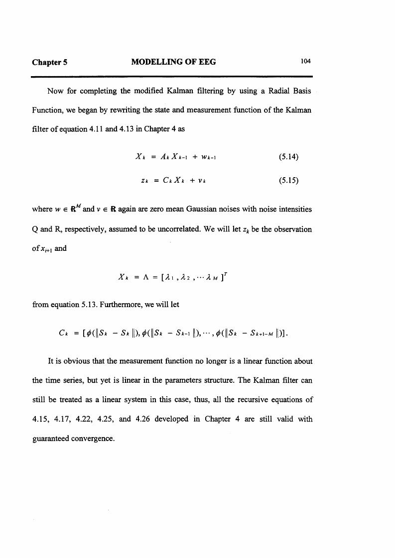
Chapter 5 MODELLING OF EEG 104
Now for completing the modified Kalman filtering by using a Radial Basis
Function, we began by rewriting the state and measurement function of the Kalman
filter of equation 4.11 and 4.13 in Chapter 4 as
X k = Ak X k - 1 + W k - \ (5.14)
Zk = Ck X k + Vk (5.15)
where w e RM and v e R again are zero mean Gaussian noises with noise intensities
Q and R, respectively, assumed to be uncorrelated. We will let zk be the observation
of :t/+I and
X k = A = [ A 1 , A 2 A m Y
from equation 5.13. Furthermore, we will let
Ck = [*(||5* -5 * | | ) , * ( | | 5 * - 5 * - i | | ) , . . . , * ( | | 5 * - 5 * +i-a#||)].
It is obvious that the measurement function no longer is a linear function about
the time series, but yet is linear in the parameters structure. The Kalman filter can
still be treated as a linear system in this case, thus, all the recursive equations of
4.15, 4.17, 4.22, 4.25, and 4.26 developed in Chapter 4 are still valid with
guaranteed convergence.

Chapter 5 MODELLING OF EEG 105
5.4.3 EEG Modelling
There are many possible choices for Radial Basis Functions as mentioned in
Chapter 4, section 4.3.5. Among them, the so called multiquadric is often the choice
in the engineering environment. That is
4>{r) = ( r 2 + c )1'2
for some constant c > 0. Gaussian and inverse multiquadric Radial Basis Function
were also under our investigation, but they do not perform so well as the
multiquadric function. Thus, in this section we will mainly discuss the performance
of multiquadric function when modelling EEG signals.
At first glance, we know that the constant c needs to be settled. Our experience
suggest that the constant c shouldn’t be too big nor too small compared with r2.
Selecting too small a value for c, the system tends to be unstable and the prediction
error increases, while too big a c setting will remarkably reduce the influence of the
Euclidean norm r between two state vectors. It is believed also that c could have a
wide range of choice if the system stability is the main consideration. Thus, we
simply select
with “( )” means average.
Chapter 5 MODELLING OF EEG 106
There are obviously other three parameters which need to be carefully selected
in this scheme. These are the order of the Kalman filter M, the embedding delay r
and the embedding dimension m'. A variety of techniques exist for the estimation of
embedding dimension, among them the most convenient technique could be via the
correlation dimension, which is a measure of the complexity and/or number of
variables required to describe the underlying dynamic system. But with the presence
of noise, this technique may not give an accurate result. Thus, based on the
performance of the scheme, we will use the prediction accuracy to estimate the
embedding dimension m' and the model order M. The mean square prediction error
for sleep stages 2 and 4 of the scheme are listed in table 5.3 and plotted in figure 5.6
and figure 5.7 for different model orders M and embedding dimensions m' settings
with r = 1. The definition of the prediction error is
£ r 2 (RBF) = <|* ( 0 - x ( 0 | 2>.
Two minutes of data, with 12 bits resolution of sleep stage 2 and sleep stage 4, are
used. To make sense of the performance, the linear Kalman filtering prediction
errors of different model order setting are also listed in table 5.3 (III) with the same
segment of EEG signals.
Finally, the performance against the embedding delay is depicted in figure 5.8
with model order M - 5 and embedding dimension m! - 5.

Chapter 5 MODELLING OF EEG 107
It is interesting to notice from figure 5.6 and figure 5.7 (or from table 5.3) that
the prediction error improves faster with embedding dimension than with model
order. It is not recommended, however, to use too low a model order, although in the
sense of the prediction error, the performance of the scheme is quite good with low
model order and high embedding dimension. That is because with too low a model
order the system tends to be unstable (adjust itself too frequently). Furthermore from
figure 5.8, it appears that the performance of the scheme wouldn’t be improved
along with the increase of the embedding delay r.

Chapter 5 MODELLING OF EEG 108
Table 5.3 (I). Mean square error of the Radial Basis Function against the model
order M and Embedding dimension m' for sleep stage 2. (See figure 5.6.)
Sleep stage 2
Order Embedding dimension rri
M 2 3 4 5 6 7 8 9 10
2 7617 5778 4596 4328 3887 3722 3691 3667 3664
3 5958 4695 4064 3798 3717 3647 3631 3599 3572
4 5434 4350 4012 3677 3646 3605 3597 3558 3520
5 5044 4374 3911 3682 3637 3610 3588 3542 3488
6 4971 4312 3896 3706 3653 3621 3587 3530 3500
7 : 4807 4245 3899 3709 3655 3620 3580 3540 3501
8 4690 4195 3869 3697 3647 3612 3587 3537 3500
9 4605 4120 3819 3680 3637 3613 3577 3526 3495
10 4468 4029 3768 3645 3652 3600 3560 3514 3489

Chapter 5 MODELLING OF EEG 109
Table 5.3 (II). Mean square error of the Radial Basis Function against the model
order M and Embedding dimension m! for sleep stage 4. (See figure 5.6.)
Sleep stage 4
Order Embedding dimension m'
M 2 Q W m 4 5 6 7 8 9 10
2 8907 6325 5549 4932 4594 4350 4146 3940 3829
3 6847 5300 4625 4277 4078 3887 3800 3605 3454
4 6081 4848 4320 3996 3847 3722 3639 3478 3419
5 5571 4602 4132 3914 3747 3653 3551 3409 3383
6 5314 4564 4033 3849 3709 3598 3501 3389 3369
7 5151 4452 4051 3837 3682 3574 3487 3389 3369
8 4921 4389 4032 3824 3683 3564 3480 3397 3381
9 4839 4342 3982 3812 3689 3576 3477 3405 3386
10 4765 4291 3978 3812 3732 3605 3496 3417 3403
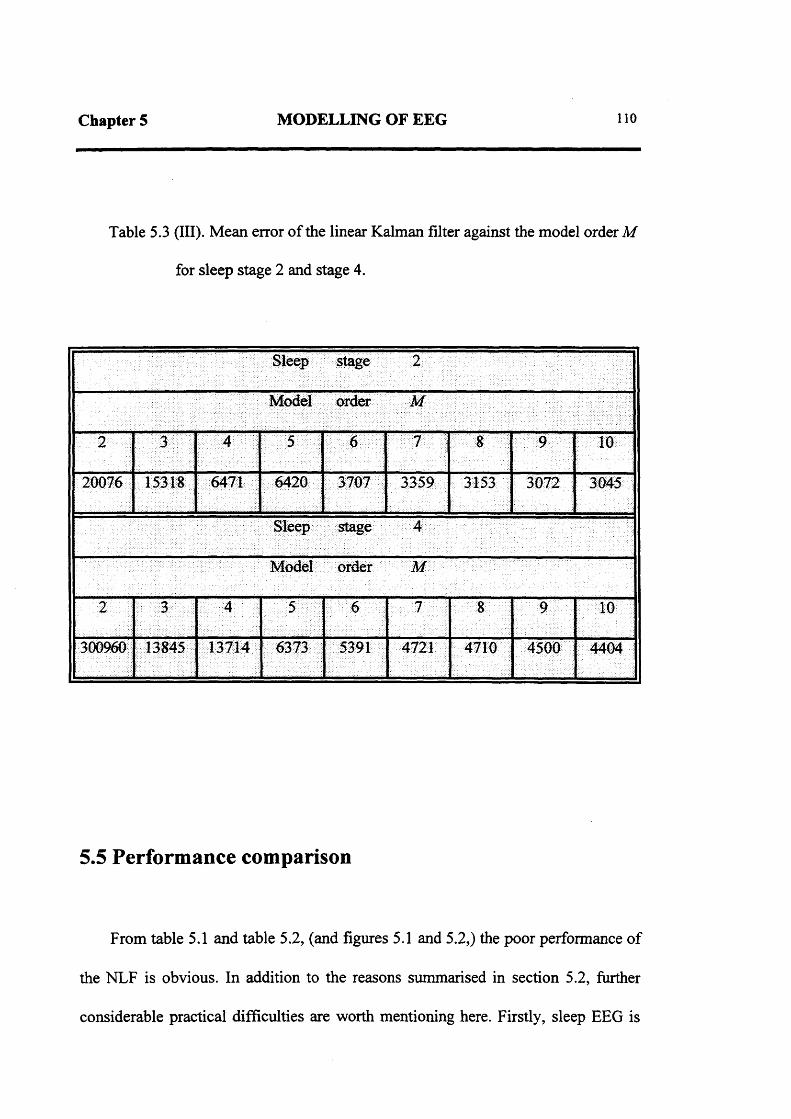
Chapter 5 MODELLING OF EEG 110
Table 5.3 (III). Mean error of the linear Kalman filter against the model order M
for sleep stage 2 and stage 4.
Sleep stage 2
Model order M
2 3 4 5 6 1 8 9 10
20076 15318 6471 6420 3707 3359 3153 3072 3045
Sleep stage 4
Model order M
2 3 5 6 8 9 10
300960 13845 13714 6373 5391 4721 4710 4500 4404
5.5 Performance comparison
From table 5.1 and table 5.2, (and figures 5.1 and 5.2,) the poor performance of
the NLF is obvious. In addition to the reasons summarised in section 5.2, further
considerable practical difficulties are worth mentioning here. Firstly, sleep EEG is

Chapter 5 MODELLING OF EEG i l l
widely believed to be unstable. In terms of dynamic systems theories, the sleep EEG
may have multi-attractors, or no definable attractors at all. That means, the
underlying dynamics evolve on the variant manifolds in a changeable dimensional
space. This violates the assumption that the attractor has an ergodic natural invariant
measure. Furthermore, there is not enough evidence for the existence of chaotic
attractors at all in some sleep stages, for example Babloyantz (1985) failed to find
them in the awake stage and the REM stage. In such a case, most non-linear analysis
of EEG signals achieved recently are dimensional (such as correlation dimension,
information dimension and etc.) and Lyapunov exponents analysis. Studies by phase
portraits can only be implemented in very short segments (only about severed tens of
seconds duration), in which the EEG can be treated as stable. Secondly, there are
difficulties of limited computer capacity. On the one hand, for example, by using
package of NLF, it costs about 20 minutes to model 1 minute EEG of sleep stage 2
(ED = 8) on a 386 personal computer. It amounts to showing that about one week
computing time would necessary to model a whole night sleep EEG (say, 8 hours),
and this is obviously unacceptable. On the other hand, memory capacity may
become unmanageable when increasing Embedding Dimension and number of Atlas
Points or using other techniques of non-linear analysis (such as global techniques
which have a very large number of free parameters to be estimated) for precise
modelling of a whole night sleep EEG. Thus it is unrealistic to precisely model a
whole night sleep EEG by using this NLF package. Table 5.2 and figures 5.1, 5.2,

Chapter 5 MODELLING OF EEG 112
5.4 and 5.5 show that the Kalman filter is much better than the Non-linear
Forecasting package for prediction.
Our results by using Radial Basis Functions are promising. As shown in table
5.3, this scheme has more or less the same prediction error as that of the Kalman
filter. Thus it could be said that the scheme seems to perform as well as the Kalman
filter in the sense of prediction error. It worth mentioning here that the scheme’s
prediction error will improve further if the multiquadric constant c is increased. But
it must be admitted at this stage that this technique is very much in its infancy. Only
the prediction errors are used for evaluation of the performance here and nothing
more. Thus, much more investigation are needed before enough confidence can be
obtained and the scheme can be used in practice.
The results of the comparative study between the non-linear prediction
technique and Kalman filtering showed that, as a predictor, the Kalman filter
approach was superior and this approach is the only choice used for the further
analysis in an attempt to classify the EEG automatically.

Chapter 5 MODELLING OF EEG 113
150
100
50
0
-50
Observed-100
Predicted
-150500 100 150 200 250
Data points
Figure 5.1. Two seconds of EEG and its prediction by using Non-linear
Forecasting package of NLF for sleep stage 4 with ED=5, PA=8000. The
ordinates are in arbitrary units.

Chapter 5 MODELLING OF EEG 114
100
-20Observed
-40 Predicted
- 60,100 150 200 250
Data points
Figure 5.2. Two seconds of EEG and its prediction by using Non-linear
Forecasting package of NLF for sleep stage 2 with ED=5, PA=8000. The
ordinates are in arbitrary units.

Chapter 5 MODELLING OF EEG 115
1.6
1.5
1.4
1.3
1.2
1.1
1
0.9
0.8
0.7
log10 (Er (KALMAN))
Sleep stage 4
Sleep stage 3
Sleep stage 2
Sleep stage 1
REM
, - L p20
Figure 5.3. Kalman filter prediction error against model order
M for 1.5 minute sections of EEG during sleep.

Chapter 5 MODELLING OF EEG 116
150
100
-50
Observed-100
Predicted
- 150,150
Data points
100 200 250
Figure 5.4. Two seconds of EEG and its prediction by using Kalman
filter modelling for sleep stage 4. The ordinates are in arbitrary units.

Chapter 5 MODELLING OF EEG 117
40
-20
Observed-40 Predicted
- 60 . 100 150
Data points
200 250
Figure 5.5. Two seconds of EEG and its prediction by using Kalman
filter modelling for sleep stage 2. The ordinates are in arbitrary units.

Chapter 5 MODELLING OF EEG 118
8000
7000
6000
5000
4000
3000
Model orderEmbedding dimension
Figure 5.6. The mean square prediction error of the modified Kalman
filter by using RBF for 2 minute section of EEG during sleep stage 2
against model order Mand embedding dimension m’ setting with
embedding delay z= 1.

Chapter 5 MODELLING OF EEG 119
9000
8000
7000
6000
5000
4000
3000
Model orderEmbedding dimension
Figure 5.7. Figure 5.6. The mean square prediction error of the modified
Kalman filter by using RBF for 2 minute section of EEG during sleep
stage 4 against model order M and embedding dimension m' setting with
embedding delay r = 1.

Chapter 5 MODELLING OF EEG 120
4800
4600
4400
4200
Sleep stage 24000
Sleep stage 4
3800
3600
T (embedding delay)
Figure 5.8. The mean square prediction error of the modified Kalman
filter by using RBF for 2 minute sections of EEG during sleep stage 2
and 4 the embedding delay with model order M - 5 and embedding
dimension rri = 5.

Chapter 6
A METHOD FOR CLASSIFYING THE
COEFFICIENTS OF THE MODEL
6.1 Introduction
As mentioned in previous chapters, the most widely used classifier following a
linear AR model is via spectrum estimation. Another widely used approach is the
use of neural networks.
The spectrum may be obtained by z-transforminf the AR model coefficients,
and all information contained in the coefficients will be transferred into the form of a
spectrum from a theoretical point of view. For sleep EEG analysis, the construction
of such a spectrum does not seem to make the analysis easier in many occasions.
The reason for this is that EEG signals, which are generated from one of the most
complicated dynamic systems, the human brain, are composed of substantial
numbers of averaged post-synaptic potentials. Thousands or even millions of

Chapter 6 A METHOD FOR CLASSIFYING THECOEFFICIENTS OF THE MODEL
122
neurones in the underlying cortex may be involved. There are good reasons to
believe that the EEG contains a vast amount of information and much of it is not just
related to sleep events. To interpret the EEG, the most important and the most
difficult job, is to extract events related information and "filter out" irrelevant
features. It seems that the main reasons for unsuccessful automatic sleep EEG
analysis are due to the failure to extract useful or relevant information and filtering
out the irrelevant features. Spectrum estimation fails to do this and it is widely
believed that no frequency band in the spectrum is actually a true sleep variable.
After spectrum estimation, researchers are still facing how to reduce the amount of
information.
Artificial neural networks seem capable of doing a good job in many practical
applications, and it seems there is a surge of interest among researchers, engineers
and industrialists. This interest is motivated by some important properties of neural
networks, such as: nonlinearity, learning capability, generalization, fault tolerance
and the ability to approximate prescribed input-output mapping of a continuous
nature. However, some of the limitations of the neural networks need to be
considered: First of all, there is much less understanding of the theory behind the
networks. Because neural networks operate as “black boxes”, i.e. their rules of
operation are completely unknown, it sometimes makes it difficult to explain the
results that are obtained from the networks. Secondly for network architecture, there
are no theoretical results nor satisfactory empirical rules suggesting how a network
should be dimensioned to solve a particular problem, such as the overall size of the

Chapter 6 A METHOD FOR CLASSIFYING THECOEFFICIENTS OF THE MODEL
123
network, the number of hidden layers and the number of neurons in each of the
hidden layers. Thirdly, convergence may also be a problem. There is no theoretical
proof at all of the convergence of the algorithm to find the coefficients, and in
practice, the most serious problem with the neural networks approach is usually the
speed of its convergence. Finally, the implementation of networks consume large
quantities of computing time as the majority of networks are simulated on sequential
machines. It is particularly true when attempting to increase the size of the networks
that the processing time requirements will increase very rapidly. Because of this
operational problem, present techniques only allow neural networks to solve fairly
small problems. In the EEG environment, there is another concern about the use of
neural networks for the classification of the different sleep stages. As mentioned in
section 2.4 of chapter 2, the criteria (i.e. R & K. rules) used contain many subjective
components and do not always provide an unequivocal basis for decision. It is a fact
that many advanced methods have been developed and have considerable potential,
the results however still do not completely correlate with the R & K standard. Thus,
it is questionable, at the present time, whether the results could be improved
significantly for classification of different sleep stages by using the input-output
mapping property of neural networks directly.
In this chapter a novel technique will be described which can provide additional
information not obtainable by manual analysis or by automatic techniques that
merely mimic the process of visual sleep staging. In this approach, dynamic systems
theory (or state-space methods) is involved for classifying AR model (Kalman filter)

Chapter 6 A METHOD FOR CLASSIFYING THECOEFFICIENTS OF THE MODEL
124
coefficients. In section 6.2, the coefficients will be embedded in a reconstructed state
space. Following this a classification of the tangent bundle will be made based on
the state changes in the EEG signals. Finally, the so called “state variable” will be
derived in section 6.4. It is considered that this state variable is generally related to
the sleep stage classified by the R & K rules.
6.2 Embedding the model’s coefficients into their state
space
After applying a Kalman filter to the EEG, it was felt reasonable to believe that
the behaviour of the five coefficients {oL(tJ} along time contained most of the useful
information in the EEG. Each coefficient was treated as a coordinate of a phase
space E = R5 (5th order Kalman filtering) and the output of the Kalman filter was
seen as a dynamic system with a point evolving on a manifold U in E. Suppose this
system is governed by an rth order differential equation, r > 1, then it can be written
as
* = X k (*)
with

Chapter 6 A METHOD FOR CLASSIFYING THECOEFFICIENTS OF THE MODEL
125
x e I I E = R 5r r
As a map, this rth order differential equation on U is a vector field
X w : T r_1 U -> T r U
on Tr_1U c R5r, after converting the original equation into a set of first order
differential equations, with T( • ) defined a tangent bundle of ( • ). This differential
equation is certainly non-autonomous as the Kalman filter is just a linear
approximation to the EEG signals and secondly, the EEG itself is an unstable signal.
A variable u e R was introduced as a measure of time to indicate that the vector
field Xu is variable with time. Thus, the differential equation can be rewritten as
X = X ( x , u )
u — 1
or X = X ( x ) (6.1)
with X = ( x , u ) .
As a map, the rth order differential equation on U can be written as a static vector
field
X :T r l U x R —>-T(Tr’ 1U x R ) = T r U x R (6.2)
o n T M U x R c R 5,+l.

Chapter 6 A METHOD FOR CLASSIFYING THECOEFFICIENTS OF THE MODEL
126
To obtain information about this dynamic system, the state space reconstruction
is necessarily the first step. As mentioned in section 4.3.2 of chapter 4, with too high
a sampling rate and too small a delay lag the method of time delays will make the
coordinates strongly correlated. This introduces an artificial symmetry into the phase
portrait and causes the trajectory to lie close to the diagonal in the embedding space.
Unfortunately this happens to be the case here. To overcome this, the method
developed in the work of Takens (1981), theorem 3 will be used. In the notation of
section 4.3.2, his theorem states that (for the dynamic systems with one observable):
Let M be a compact manifold of dimension d. For pairs f t h\fa . smooth vector field
and h a smooth function on M, it is a generic property that the map
O / ,h : M -» R2̂ 1, defined by
(5) = (* (* ) , T r W ' i ' ' (* )» . (»))) )i=o d t ,=0
(6.3)
is an embedding, Here vp/ (again) denotes the flow of/; this time, smooth means at
least C2̂ 1.
This theorem tells us that state space reconstruction could be achieved by
implementing this derivative map O / ,h. Thus, in our case, to reconstruct the state
space of the dynamic system of equation 6.1, one can embed the model’s
coefficients {aft)}, in a space of

Chapter 6 A METHOD FOR CLASSIFYING THECOEFFICIENTS OF THE MODEL
127
d d2r( « ( t i ) > T T a ( n )>•• >------7 7 a ( ?i ) ) x R ( 6 -4 )At d t 2
with a(^) being a vector of dimension 5. For convenience, the state space will be
represented as the form of tangent bundle. Thus, the state space of equation 6.4 can
qbe written as T UxR with q = 2r.
6.3 Classifying the model’s coefficients
The derivative mapping O gives an important equivalent relation between the
manifold in the state space and the original dynamic system (equation 6.1). Thus, it
is reasonable to say that the state space contains all the information which Kalman
coefficients have if q is fairly high. Therefore it is possible to find some way of
classifying a model’s coefficients in state space according to some state changes of
EEG signals. That is, to find some equivalence relation Q defined on T UxR based
qon some sleep events, then Q gives a decomposition of T UxR into a quotient space
(T ,UxR)/Q.
It was found that the manifold U c E i s kept unchanged along the whole night
sleep, except during the wake stage and movement arousal. However, the system
image in the space of TUxR (i.e. q = 1) or more efficiently in (TUxR)/V does vary

Chapter 6 A METHOD FOR CLASSIFYING THECOEFFICIENTS OF THE MODEL
128
with the deepness of the sleep if V denotes the relation of all points p in the manifold
U that are equivalent. Space (TUxR)/V in fact comes from a projection n from TUx
R onto an arbitrary tangent space TpUxR, as shown in figure 6.1 below and it gives
ideas only about the velocity (a vector) of the point moving round in the manifold U.
(TUXR)/V
Projection
71
TUXR
TPUXR
XUXR
Figure 6.1. Space (TUxR)/V is a quotient space of TUxR. V denotes
the equivalent relation of all points p in the manifold U.
Statistics analyses were carried out in the space TU/V for different sleep stages
and it was turn out that the direction of the velocity appear to be random. As an
example, figure 6.2 shows how the system behaved in the space TU/V of dimension
5. One and half minute of data are used in this example and only three projections
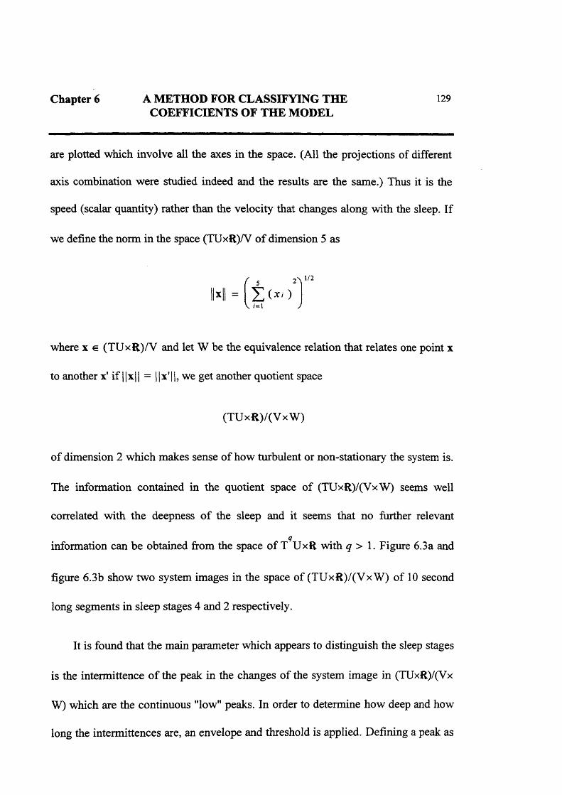
Chapter 6 A METHOD FOR CLASSIFYING THECOEFFICIENTS OF THE MODEL
129
are plotted which involve all the axes in the space. (All the projections of different
axis combination were studied indeed and the results are the same.) Thus it is the
speed (scalar quantity) rather than the velocity that changes along with the sleep. If
we define the norm in the space (TUxR)/V of dimension 5 as
x =2\ 1/2
where x e (TUxR)/V and let W be the equivalence relation that relates one point x
to another x’ if ||x || = ||x '||, we get another quotient space
(TUxR)/(VxW )
of dimension 2 which makes sense of how turbulent or non-stationary the system is.
The information contained in the quotient space of (TUxR)/(VxW) seems well
correlated with the deepness of the sleep and it seems that no further relevant
qinformation can be obtained from the space of T UxR with q > 1. Figure 6.3a and
figure 6.3b show two system images in the space of (TUxR)/(VxW ) of 10 second
long segments in sleep stages 4 and 2 respectively.
It is found that the main parameter which appears to distinguish the sleep stages
is the intermittence of the peak in the changes of the system image in (TUxR)/(Vx
W) which are the continuous "low" peaks. In order to determine how deep and how
long the intermittences are, an envelope and threshold is applied. Defining a peak as
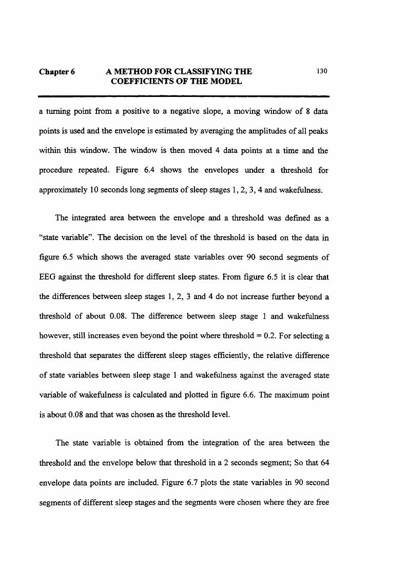
Chapter 6 A METHOD FOR CLASSIFYING THECOEFFICIENTS OF THE MODEL
130
a turning point from a positive to a negative slope, a moving window of 8 data
points is used and the envelope is estimated by averaging the amplitudes of all peaks
within this window. The window is then moved 4 data points at a time and the
procedure repeated. Figure 6.4 shows the envelopes under a threshold for
approximately 10 seconds long segments of sleep stages 1, 2, 3, 4 and wakefulness.
The integrated area between the envelope and a threshold was defined as a
“state variable”. The decision on the level of the threshold is based on the data in
figure 6.5 which shows the averaged state variables over 90 second segments of
EEG against the threshold for different sleep states. From figure 6.5 it is clear that
the differences between sleep stages 1, 2, 3 and 4 do not increase further beyond a
threshold of about 0.08. The difference between sleep stage 1 and wakefulness
however, still increases even beyond the point where threshold = 0.2. For selecting a
threshold that separates the different sleep stages efficiently, the relative difference
of state variables between sleep stage 1 and wakefulness against the averaged state
variable of wakefulness is calculated and plotted in figure 6.6. The maximum point
is about 0.08 and that was chosen as the threshold level.
The state variable is obtained from the integration of the area between the
threshold and the envelope below that threshold in a 2 seconds segment; So that 64
envelope data points are included. Figure 6.7 plots the state variables in 90 second
segments of different sleep stages and the segments were chosen where they are free

Chapter 6 A METHOD FOR CLASSIFYING THECOEFFICIENTS OF THE MODEL
131
from noise and artifacts, such as the high frequency noise from EMG channel and
movement artifact.

Chapter 6 A METHOD FOR CLASSIFYING THECOEFFICIENTS OF THE MODEL
132
axis2
1.5
1
0.5
0
-0.5
-1
-1.5
-2 -1.5 -1 -0.5 0 0.5 1 a x is l(a)
ax is4
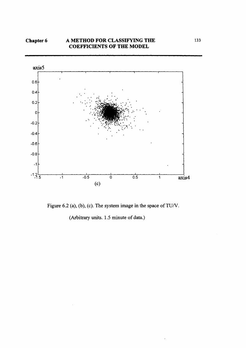
Chapter 6 A METHOD FOR CLASSIFYING THECOEFFICIENTS OF THE MODEL
133
axis5
0.6
0.4
0.2
0
- 0.2
-0.4
- 0.6
- 0.8
-1
"1- .̂5 -1 -0.5 o 0.5 1 axis4(c)
Figure 6.2 (a), (b), (c). The system image in the space of TU/V.
(Arbitrary units. 1.5 minute of data.)

Chapter 6 A METHOD FOR CLASSIFYING THECOEFFICIENTS OF THE MODEL
134
Data points1200
Figure 6.3a. The system image in the space of
(TUxR)/(Vx W) for sleep stage 4 in arbitrary units. (10 seconds of data.)
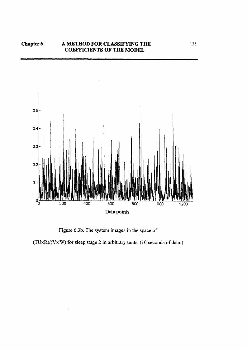
Chapter 6 A METHOD FOR CLASSIFYING THE 135COEFFICIENTS OF THE MODEL
0.5
0.4
0.3
Data points
Figure 6.3b. The system images in the space of
(TUxR)/(VxW) for sleep stage 2 in arbitrary units. (10 seconds of data.)
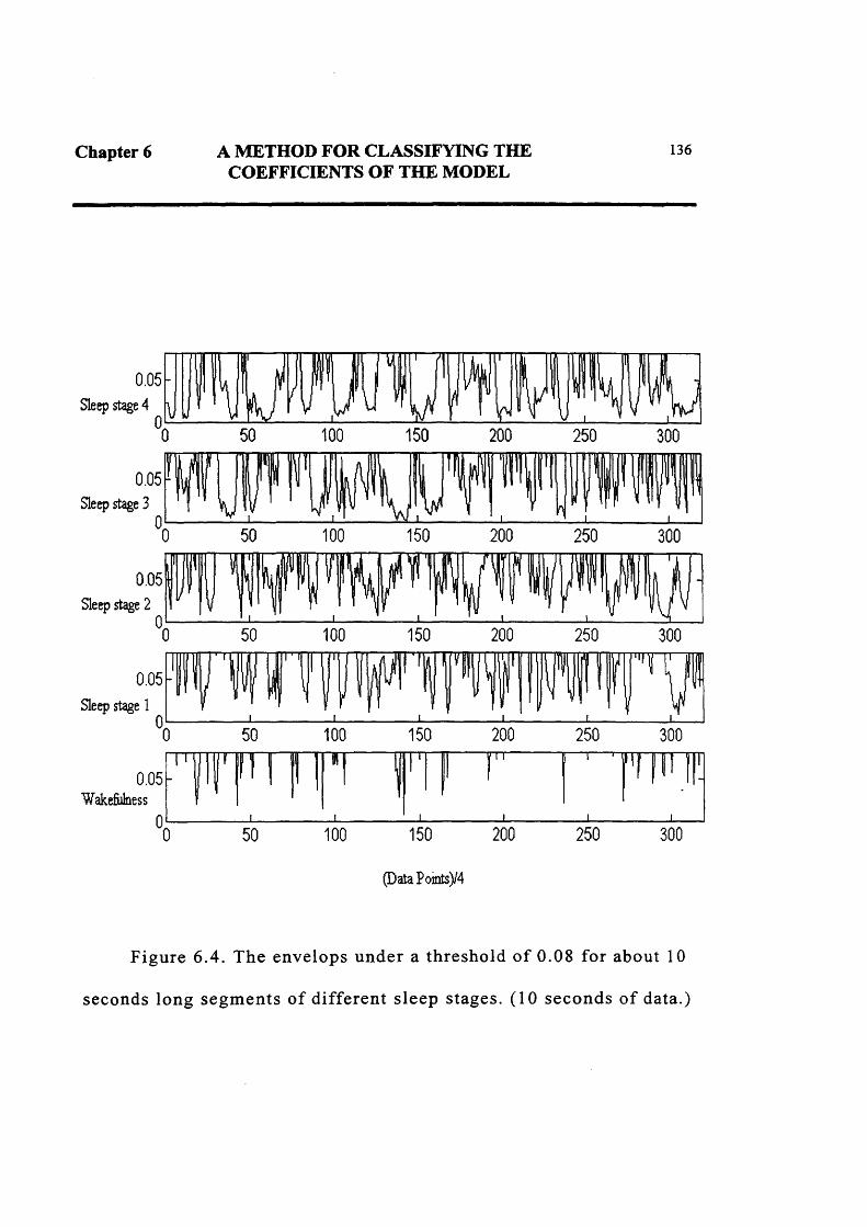
Chapter 6 A METHOD FOR CLASSIFYING THECOEFFICIENTS OF THE MODEL
136
0.05Sleep stage 4
100 150 200 250 300
0.05 Sleep stage 3
150100 200 250 300
0.05 Sleep stage 2
0 50 100 150 200 250 300
Sleep stage 1
*0 50 100 150 200 250 300
(DataPoints)/4
Figure 6.4. The envelops under a threshold o f 0.08 for about 10
seconds long segm ents o f d ifferen t sleep stages. (10 seconds o f data.)

Chapter 6 A METHOD FOR CLASSIFYING THECOEFFICIENTS OF THE MODEL
137
6 Wakefulness
Sleep stage 1
Sleep stage 2
++ +++ Sleep stage 3
Sleep stage 4
5
4
3
2
1
0.0.1 0.150.050 0.2 0.25
Threshold level
Figure 6.5. Averaged state variable (in arbitrary units) over one and half
minutes long EEG segments against threshold level.

Chapter 6 A METHOD FOR CLASSIFYING THECOEFFICIENTS OF THE MODEL
138
0.5
- 0.5
0.05 0.1 0.15 0.2 0.25
Threshold level
Figure 6.6. Relative difference of state variables between
sleep stage 1 and wakefulness in arbitrary units.

Chapter 6 A METHOD FOR CLASSIFYING THECOEFFICIENTS OF THE MODEL
139
40
Stage 4
20
0
Stage 4
40
Stage 3
20
0
40
Stage 2
20
0
Stage 1
0 10 20 30 40
40
WakefulnessArtifact
20
0
1.5 minute segments
F ig u re 6 .7 . T he s ta te v a r ia b le s fo r d if f e re n t s leep
s ta g e s . (E ach d a ta is g e n e ra te d from a 2 sec o n d s ep o ch .)

Chapter 7
RESULTS
A pilot study of analysis of the human sleep continuum has been numerically
presented in previous chapters — Model based dynamic analysis, in which the EEG
signal is first characterized by using adaptive AR model (Kalman filter), and then
the model coefficients are analysed dynamically. In figure 6.6 (in chapter 6), the
state variable appears to vary with different sleep stages. To demonstrate the
potential usefulness of the approach, the behaviour of the state variable across a
whole night will be analysed in this chapter.
Figure 7.1 presents the performance of the state variable for the whole night
recording from which the method was developed (i.e. the same sleep EEG of figure
6.6 ). Figure 7.2 indicates the manually scored hypnogram of the same sleep as of
figure 7.1. It is encouraging to observe that the state variable appears to be correlated
with the depth o f the sleep.
A further method of demonstration the correlation is to average the state
variable in each (30 or 20 second) epoch, as shown in figure 7.3, and then to analyse

Chapter 7 RESULTS 141
the distribution of the averaged state variable within each manually scored sleep
stage. To check this pilot study a different record (of subject 2 if the subject 1 was
used for the pilot study) from the same data source is also used for the further studies
(see APPENDIX B for more details about each record). Figure 7.4 shows the
averaged state variable with the whole night sleep of the subject 2 and the visually
scored hypnogram. To analyse the distribution of the state variable within each sleep
stage, the averaged state variable of subject 1 and 2 against the manually scored
sleep stage for the same epoch are plotted in figure 7.5. For a perfect agreement, one
would expect that the points in figure 7.5 would fall on a diagonal line. There are
three reasons why this is not the case. Firstly, the state variable is a continuous
parameter, whilst the manually scored sleep stages are discrete. Thus it is inevitable
that the image in figure 7.5 has an cascade-like structure. Discretization of human
sleep has been considered as one of the major shortcomings of the rules used in sleep
analysis. Secondly, the rules used to score the sleep stages have arbitrarily-defined
thresholds. For example, scoring of sleep stage 2 is mainly based on very short
duration events such as K-complexes and sleep spindles (each of which are about
half second duration). Scoring of stage 3 requires 20 - 50% of the delta activity
during an epoch with a frequency of 2 Hz or lower and a peak-to-peak amplitude of
75 fiV or higher in the EEG channel. A subjective assessment of the EEG is
therefore required when applying the rules and this can lead to unreliable results and
poor agreement between scorers (Kelley et al. 1985). Thirdly, the noise contained in
the EEG channel contributes to the scatter of the points in figure 7.5. Close study

Chapter 7 RESULTS 142
shows that most, if not all, of the outlying peaks and troughs in figure 7.1, 7.3 and
7.4(a) are caused by noise. When a low frequency artifact appeared in the EEG
channel caused by a body movement, there will be a considerable high peak in these
figures. When there is high frequency noise, such as in a case of a micro-arousal, a
significant trough will present. It may also worth to note that the manual observer
tends to assume that a state persists when he/she assesses a sleep record, i.e.
“expected stage” depends upon previous decisions. While, the model based dynamic
analysis makes no such assumption and evaluates each epoch independently. This
may also contribute to the scatter of the points in figure 7.5.
Figure 7.5 indicates also that the state variable has better agreement within
stages of NREM sleep than during REM sleep and MT (Movement Time) stages.
This may happen because REM sleep is mainly characterized by bursts of rapid eye
movement and suppression of EMG activity, whilst the EEG pattern resembles that
of the stage 1. In MT stage the EEG tracing is normally obscured for at least half the
epoch by muscle tension and/or amplifier blocking artifacts associated with
movement of the subject. Thus the state variable is expected to be scattered over a
wide range.
For further analysis of the distribution of the state variable in each sleep stage, a
group of figures are produced. Figure 7.6 and 7.8 demonstrate the distribution, non
normalized and normalized, of the averaged state variable for different NREM sleep
stages (sleep stage 1, 2, 3 and 4) of subject 1 and 2, followed by figure 7.7 and 7.9,

Chapter 7 RESULTS 143
in which the normalized distributions of the averaged state variable are separately
plotted again in different NREM sleep stages. It appears that the means of the state
variable for each sleep stage can be distinguished but there are overlaps of the
distribution among them. It is believed that the arbitrary way the R and K rules are
defined, the subjective assessment of the EEG, as mentioned above, and the noise
contained in it may be among the main reasons for the overlapping. To further
demonstrate the consistency of the technique over different subjects, the state
variable against each subject in each sleep stage are plotted in figure 7.10. It appears
the technique has a good consistency within these two subjects.
Four more overnights’ sleep from different data source have been analysed in
this way to gain more insight into the distribution and overlaps of the state variable.
This makes a total of six night’s sleep altogether and it may be enough to examine
overall values of the technique. The records are divided into two groups based on the
two data sources. The two records in the first group, i.e. subject 1 and 2, are visually
staged in the Department of Engineering Science, Oxford University and 30 second
epochs are used. The second group of records of subject 3 to 6 are manually assessed
by Jane Jones (NCE Brainwaves, N. Ireland) and 20 second segments are employed.
The way the EEG signals are digitized is also different in these two groups (for more
details see Appendix B). In the first group, the EEG signals were digitized using 8
bit resolution and the remainder were digitized in 12 bit. Thus the second group of
data has the following characteristics; it is of better amplitude resolution, better time

Chapter 7 RESULTS 144
resolution and more consistent scoring (four sleeps were staged by one scorer). All
the results are presented in the following figures (figure 7.11- 7.24).
Figure 7.11, 7.12, 7.13, and 7.14 show the averaged state variable for the whole
night sleeps of the 4 additional subjects (subject 3 to 6) and their manually scored
hypnogram s. The averaged state variable of each subject against sleep stages are
plotted in figure 7.15, (the terms “U”, “N” and “C” are described below) and the
distribution and normalized distribution of the state variable for subject 3 to 6 are
presented in figure 7.16, 7.18, 7.20, and 7.22. Again, the normalized distribution in
different NREM sleep stages are separately displayed in figure 7.17, 7.19, 7.21 and
7.23. The consistency of the distribution of the state variable against each subject in
each sleep stage are plotted in figure 7.24. Comparing the two groups of sleep, it
appears that the image of the averaged' state variable in the second group (in figure
7.11(a), 7.12(a), 7.13(a) and 7.14(a)) have more hair-like peaks than that of the first
group (figure 7.3 and 7.4(a)). The main reason is that a 20 second epoch is used in
the second group, whilst a 30 second epoch is used for the first.
A confidence factor is also given in scoring the second group of sleep along
with sleep stages. For each epoch, not only is a sleep stage attached by the scorer,
but also a factor o f confidence. As shown in figure 7.15 the factor involves three
levels, in which U means “uncertain”, N means “normal”, and C means “certain”.
Only the epoch with confident factors of certain are used in the following analysis of
the state variable distribution. Because of the difference in digitized resolution, the

Chapter 7 RESULTS 145
ranges of the state variable therefore are different in the two groups of sleep. This
would not appear to be a problem as only relative values of the state variable are of
interest in this analysis. If many different sources were used then a normalization
procedure on the raw data could be used to make all data comparable.
The results shown in the figures mentioned above suggest that the state variable
behaved in the same manner in the six different sleeps, and it is well correlated with
the depth of the sleep. The distributions of the state variable did not appear to be
significantly different in different sleeps. If there are differences, they may be in the
mean distribution of state variable in stage 3 and the range in stage 2. The mean
distribution in stage 3 seems slightly closer to that of sleep stage 2 in the first group
of sleeps, and the distribution range in stage 2 in second group seems wider than that
in first group. The reason for this is not clear, but it is believed that the reason is the
arbitrarily-defined thresholds on sleep stage 2 and subjective assessment of the EEG
when applying the rules.
It is notable that the sleeps of subject 5 and 6 have very little sleep stage 4 (two
epochs of sleep stage 4 for subject 5 and none for subject 6), Thus these may not be
normal sleeps, but the technique still works well. Since there is not enough stage 4 in
subjects 5 and 6, it is hard to evaluate the consistency of the state variable in this
stage. But based on the previous analysis, it seems to have a good ability to separate
sleep stage 4 from other stages, as shown in figure 7.6, 7.8, 7.16, and 7.18. The
consistency in sleep stage 2 and 3 as shown in figure 7.24 appears good, although it

Chapter 7 RESULTS 146
appears that the state variable has a wider range in the second group of stage 2. The
consistency among the different subjects in sleep stage 1 appears not so good in the
second group of recordings. Obviously, stage 1 is a light sleep, more noise is caused
by movement and arousals in this stage, therefore the distribution of the state
variable scattered by the noise contained in the EEG leads to poor consistency
among different subjects.

Chapter 7 RESULTS 147
State variable
Time (minutes)
F igure 7.1. State variab le for a whole n ig h t’s sleep o f
sub ject 1. (Each data is generated from a 2 seconds
epoch.)

Chapter 7 RESULTS 148
Stage 4
Stage 3
Stage 2
Stage 1
REM
MT
Wake
10050 150Time (minutes)
200 250
F igure 7.2. V isually scored hypnogram o f the same sleep as
figure 7.1. (30 seconds epoch.)

Chapter 7 RESULTS 149
State variable
35
30
25
20
15
10
5
Epoch =
6000.
1000 200 300 400 500
Figure 7.3. Averaged state variable within the same sleep as o f
figure 7.1.

Chapter 7 RESULTS 150
State variable
30
25
20
100 200 300 400 500 600 700 800 900
Sleep stage
Stage 4
Stage 3 -
Stage 2
Stage 1
REM
W ake
Epoch = 30s
900200 300 4000 100 500 600 700 800
Figure 7.4. (a) Averaged state variable for a whole n ig h t’s
sleep of subject 2 and (b) its v isually scored hypnogram .

Chapter 7 RESULTS 151
- State variable0
5
-10
-15
-20
-25
-30
Sleep stage- 35.0 WakeMTStage 4 Stage 3 Stage 2 Stage 1 REM
- State variable
-10
-15
-20
-25
-30
Sleep stage-35
WakeMTStage 4 Stage 3 Stage 2 Stage 1 REM
Figure 7.5. Averaged state variable against sleep stages for subject 1 (a)
and subject 2 (b).

Chapter 7 RESULTS 152
Number45 Stage 2
40
35
30
25
20 Stage 4
Stage 3
10
Stage 1
20 2515 30State variable
Normalized distributionState 20.25
State 3State 1 -I
0.2
State 4
0.15
0.1
0.05
0, 10 2015 255 300 35State variable
Figure 7.6. Distribution (a) and normalized distribution (b) of averaged
state variable for different NREM sleep stages of subject 1.
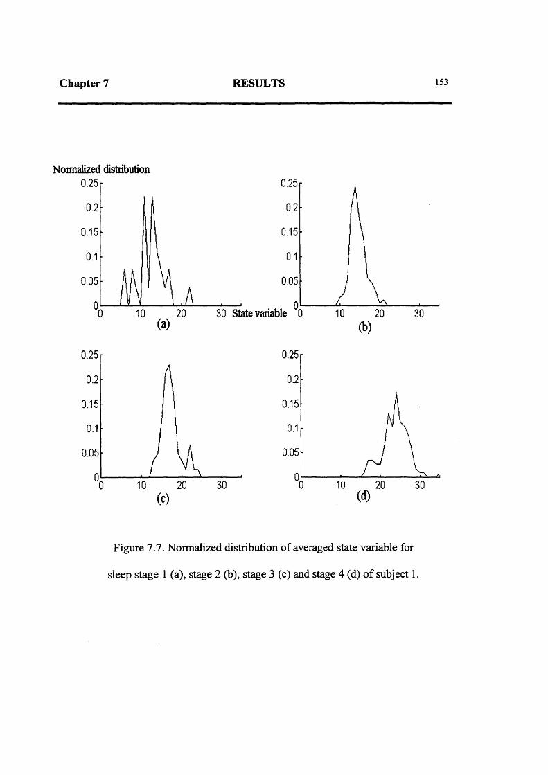
Chapter 7 RESULTS 153
Normalized distribution0.250.25
0.150.15
0.050.05
30 State variable 0(a)
0.25 r
0.15
0.05
0.25r
0.2
0.15
0.05
Figure 7.7. Normalized distribution of averaged state variable for
sleep stage 1 (a), stage 2 (b), stage 3 (c) and stage 4 (d) of subject 1.

Chapter 7 RESULTS 154
Number
140Stage 2
120
100
80
60
40 -
Stage 4Stage 320
Stage 1v -
10 20 25 30 35State variable
Normalized distribution
Stage 20.35 r
0.3
Stage 30.25
0.2Stage 4
0.15Stage 1
0.05
20 30 35State variable
Figure 7.8. Distribution (a) and normalized distribution (b) of averaged
state variable for different NREM sleep stages of subject 2.

Chapter 7 RESULTS 155
Normalized distribution
0.250.25
0.150.15
0.050.05
30 State variable 0(a) <b)
0.25
0.15
0.05
0.25-
0.15
0.05
Figure 7.9. Normalised distribution of averaged state variable for sleep
stage 1 (a), stage 2 (b), stage 3 (c) and stage 4 (d) of subject 2.
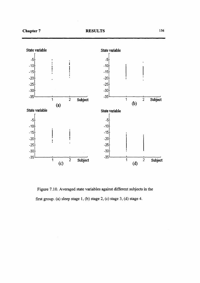
Chapter 7 RESULTS 156
State variable
-5 -10
-15 -20
-25 -30 -35
(a)Subject
State variable
-10
-15-20-25-30-35
2 Subject
State variable
-5 -10
-15 -20 -25 -30 -35
(b)Subject
State variable
-5 -10
-15 -20 -25 -30 -35
1 2 Subject
Figure 7.10. Averaged state variables against different subjects in the
first group, (a) sleep stage 1, (b) stage 2, (c) stage 3, (d) stage 4.

Chapter 7 RESULTS 157
State variable
Sleep stage
Stage 4
Stage 3
Stage 2
Stage 1
REM
MT
W ake
0
Epoch = 20s
I]
Epoch = 20s
500(b)
1000 1500
Figure 7.11. (a) Averaged state variable for a whole night’s sleep of
subject 3 and (b) its visually scored hypnogram.

Chapter 7 RESULTS 158
State variable60
1000
Epoch = 20s
1400
Sleep stage
MT
Wake
Epoch = 20s
200 400 600 800(b)
1000 1200 1400
Figure 7.12. (a) A veraged sta te variable for a whole n ig h t’s
sleep of subject 4 and (b) its v isua lly scored hypnogram .

Chapter 7 RESULTS 159
State variable
60 r
50 -
0<------------ 1-------------1------------ 1-------------1------------ 1________ i________ i0 200 400 600 800 1000 1200 1400
(a)Sleep stage
Stage 4
Stage 3
Stage 2
Stage 1
REM
M T
W ake
800200 400 600 10000 1200(b)
Figure 7.13. (a) A veraged sta te variab le for a w hole n ig h t’s
sleep of subject 5 and (b) its v isually scored hypnogram .
20s
= 20s

Chapter 7 RESULTS 160
State variable
Sleep stage
400 600 800 (a)
1000 1200
Epoch = 20s
1400
Stage 4
Stage 3
Stage 2
Stage 1
REM
MT
Wake
0 200 400 600 800 1000 1200 1400(b)
Figure 7.14. (a) A veraged state variable for a whole n ig h t’s
sleep of subject 6 and (b) its v isually scored hypnogram .

Chapter 7 RESULTS 161
- State variable
-10 U N C
-20
-30
-40 UncertainNormalCertain
-50
Sleep stage-60
WakeStage 4 Stage 3 Stage 2 Stage 1 REM MT
- State variable
-10
-20
-30
-40U — Uncertain N — Normal C — Certain
-50
Sleep stage-60
WakeStage 4 Stage 3 Stage 2 Stage 1 REM MT
Figure 7.15. Averaged state variable against sleep stages, (a) subject 3, (b) subject 4.
(Subjects 5 and 6 are shown on the next page.)

Chapter 7 RESULTS 162
- State variable
-10
-15
-20
-25
-30
-35 UncertainNormalCertain-40
-45Sleep
-50WakeStage 4 Stage 3 Stage 2 Stage 1 REM MT
- State variable
-10
-20
-30
-40U — Uncertain N — Normal C — Certain-50
-60WakeStage 4 Stage 3 Stage 2 Stage 1 REM MT
Figure 7.15 contiune. Averaged state variable against sleep stages,
subject 4, (c) subject 5, (d) subject 6.

Chapter 7 RESULTS 163
Number60
Stage 250
40
20Stage 3
Stage 4Stage 110
4020 50State variable
Normalized distribution
0.18
0.16Stage 4Stage 1
0.14
Stage 30.12
0.1Stage 2
0.08
0.06
0.04
0.02
40 50State variable
Figure 7.16. (a) Distribution and (b) normalized distribution of
averaged state variable for different NREM sleep stages of subject 3.

Chapter 7 RESULTS 164
Normalized distribution0.1
0.08
0.06
0.04
0.02
0,0 20 6040
0.15
0.05
State variable
0.2
0.1
00 20 40 60
0.12
0.08
0.06
0.04
0.02
Figure 7.17. Normalized distribution of averaged state variable for sleep
stage 1 (a), stage 2 (b), stage 3 (c) and stage 4 (d) of subject 3.

165r e s u l t s _
Chapter 7 _------ .--------- '
Stage 2
45
40
Stage 3Stage 4
Stage 1
State variable
Normalized DistributionStage 3
Stage 4
Stage 2
S tagel
0.08
0.06
0.04
0.02
State variable40
Figure 7.18. (a) Distribution and (2) no
state variable for
irmalized distribution of averaged
different NREM sleep stages of subject 4.

Chapter 7 RESULTS 166
Normalized distribution0.12
0.1
0.08
0.06
0.04
0.02
00 20 40 60
0.08
0.06
0.04
0.02State variable
0.15
0.1
0.05
00 20 40 60
0.15
0.05
Figure 7.19. Normalized distribution of averaged state variable for sleep
stage 1 (a), stage 2 (b), stage 3 (c) and stage 4 (d) of subject 4.

Chapter 7 RESULTS 167
Number60
50 Stage 2
40
30
20
Stage 1Sleep stage 4
Stage 3 / V
4020 50 60(a) State variable
Normalized distributionStage 4
0.9
0.8
0.7
0.6
0.5
0.4
0.3 Stage 1;;Stage 3
0.2
Stage 2
20 30 40 5010 60State variable
Figure 7.20. (a) Distribution and (b) normalized distribution of averaged
state variable for different NREM sleep stages of subject 5.

Chapter 7 RESULTS 168
Normalized distribution
0.4 r
0.3
0.2
State avriable
0.08
0.06
0.04
0.02
0.2 1
0.8
0.6
0.4
0.2
00 20 (d) 40 60
Figure 7.21. Normalized distribution of averaged state variable for sleep
stage 1 (a), stage 2 (b), stage 3 (c) and stage 4 (d) of subject 5.

Chapter 7 RESULTS 169
Number60 r
Stage 250
40
Stage 1
Stage 3
40 50State variable
NormaHzed distribution
Stage 3
Stage 10.1
0.08
Stage 20.06
0.04
0.02
30 40 50Stage variable
Figure 7.22. (a) Distribution and (b) normalized distribution of averaged
state variable for different NREM sleep stages of subject 6.

Chapter 7 RESULTS 170
Normalized distribution0.08
0.06
0.04-
0.02
0.12
0.08
0.06
0.04
0.02State variable
0.12
0.08-
0.06
0.04
0.02
Figure 7.23. Normalized distribution of averaged state variable for
sleep stage 1 (a), stage 2 (b) and stage 3 (c) of subject 6.
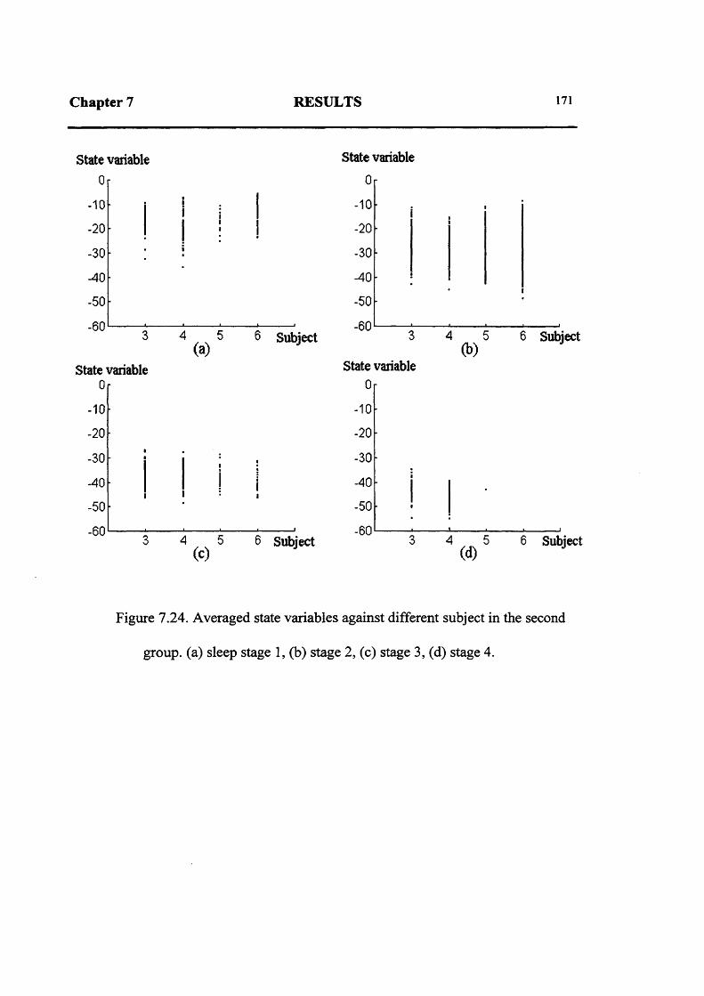
Chapter 7 RESULTS 171
State variable0
-10
-20
-30
-40
-50
-60
State variable
4 5(a)
6 Subject
-10
-20
-30
-40
-50
-606 Subject
State variable
Or
-10
-20
-30
-40
-50
-60
State variable
4 5(b)
6 Subject
-10
-20
-30
-40
-50
-606 Subject
Figure 7.24. Averaged state variables against different subject in the second
group, (a) sleep stage 1, (b) stage 2, (c) stage 3, (d) stage 4.

Chapter 8
CONCLUSIONS AND FURTHER WORK
Traditionally, the most important aspect of sleep analysis is sleep staging. For
sleep staging, EEG signals are usually recorded in order to obtain relevant
information about the process of the sleep. However, inevitably, this information is
hidden in noise. These neurophysiological signals are recorded at a rate of over a
hundred samples per second and sometimes over a number of channels together with
the EMG and/or EOG signals. Both data reduction and extraction of the relevant
information are therefore common goals of most automatic analysis methods. To
achieve these, feature extraction from the EEG (EEG interpretation) followed by
features classification are the procedures included in most of the automatic methods.
8.1 EEG interpretation
There are many existing techniques for the interpretation of EEG signals.
Among them, the most commonly used in EEG processing are the frequency domain

Chapter 8 CONCLUSIONS AND FURTHER WORK 173
methods (or transfer-function models). In frequency domain analysis the EEG waves
are treated as a collection of periodic signals, with an assumption that the underlying
system is linear and time invariant system. This is often far from reasonable in the
EEG environment. The realization that deterministic chaos may be generated from
rather simple deterministic dynamics led to the search for non-linear dynamic
systems in the area of EEG analysis.
To release these assumptions imposed on the frequency analysis, a state space
approach (rather than transfer-function modelling) for EEG interpretation has been
used in this project, since state space modelling has many distinct advantages over
transfer-function techniques. One of the most important advantages may be that the
state space methods can be easily generalized. Thus they have the capability to
characterize a non-linear, time varying, or nonstationary random system.
In this project, the performance of three kinds of state space approaches
(described in chapter 5) was investigated, i.e. one linear and two non-linear models
for modelling and forecasting the electroencephalogram (EEG) during sleep. Firstly
in section 5.2, the non-linear local prediction technique of Schaffer and Tidd (1990),
known as NLF, was investigated. This technique treated the EEG signals as
generated from a non-linear but stationary system. Secondly in section 5.3, a linear
state space approach of the so called Kalman filtering technique was implemented.
As Kalman filters have the ability of self-adaptation along changes of signal
properties, they have the capability to characterize time varying systems. Finally, a

Chapter 8 CONCLUSIONS AND FURTHER WORK 174
recursive version of the Radial Basis function scheme was considered in section 5.4.
In the scheme developed here, the structure of a Kalman filter was adopted, but
Radial Basis Functions were introduced into the measurement function. It could
therefore be treated as a non-linear, time varying approach.
To evaluate the performance of NLF in EEG analysis, the Normalised Predictor
Error (NPE) of NLF with different parameter settings of sleep stage 4 and 2 were
compared in chapter 5 along with two simple predictors (zero and first order
polynomial analysis). It was clear that the NLF, with the embedding dimension set
to 2, is only marginally better than the first order linear predictor. It was expected
that NLF would perform better with higher settings of the embedding dimension as
EEG signals are considered to have high dimensional properties (B. Doyon, 1992).
However, this was not the case as performance worsened as the embedding
dimension was increased. The results also suggest that increasing the Atlas Points
would not be o f any benefit. This behaviour of the NLF is mainly because of the
unstable and noisy properties of the EEG signals. NLF treated the signals as
generated from a stationary system and it had no ability to filter out any noise which
corrupted the signals. As many non-linear system analysis techniques are very
susceptible to noise, it may be the main reason that the success of applying chaos
theory (non-linear system analysis) to most natural phenomena has been much
slower than that of well-controlled and somewhat artificial laboratory experiments
and why many algorithms available for analysis of chaotic time series are of limited
practical use. Among other reasons may be the limited capacity of the NLF package

Chapter 8 CONCLUSIONS AND FURTHER WORK 175
which limits the maximum number of points to 10000. Compared with Kalman
filtering of order 5 the unsatisfactory performance of the NLF is evident.
Linear approximation is an important tool for analysing a non-linear system.
Kalman filters, as linear state space representations, have an advantage over classical
transfer function methods, i.e. they have the ability of adaptation to changes of
signal properties. Thus they are superior, in principle, to other AR models, can
sometimes be quite well behaved when applied to chaotic systems, and they have
been widely applied in various areas to estimate the states of non-linear systems
(e.g., Mous and Grasman, 1983; Bockman, 1991; Myers et. al., 1992). But it seems
that the superior potential of Kalman filters have not been fully exploited in EEG
analyses. In practice, most researchers have used Kalman filters as a first step toward
spectrum estimation, for spectrum estimation however higher model orders are
needed while Kalman filters are sensitive to the model order and with too high a
model order (indicated by the FPE criterion) Kalman filters may produce spurious
peaks in the spectra. It is suggested in this work that a different approach for EEG
classification can be used which is not based on spectral estimation and does not
favour any particular model order. In this way, a model order somewhat lower than
the “best order” for the spectral estimation approach can be used and it is shown that
such low model order Kalman filters are used for analysing EEG signals, making it
possible to use a short segment length. Thus from an engineering point of view,
there is an advantage in using such a short segment length to deal with unstable

Chapter 8 CONCLUSIONS AND FURTHER WORK 176
system like EEG and in clinical point of view, it makes possible the unmasking of
micro-arousals.
The use of Radial basis functions for modelling EEG signals was also
considered. In the literature of approximation theory, Radial basis function
techniques are solutions to real multivariable interpolation problems. This approach
to multivariable interpolation provides a highly promising way of dealing with
irregularly positioned data points. One disadvantage of this procedure is that the
parameters have to be calculated once and for all and this was shown to be quite
time consuming. Therefore this algorithm is not particularly suited for real-time
application. Another major disadvantage of this procedure is that it has no ability for
modelling signals with noise superimposed. Therefore, a modified Kalman filtering
approach was proposed in which Radial Basis Functions were introduced and led to
a recursive version of the scheme that continuously updated the parameters using
incoming values of the time series. This resulted in an algorithm much more
appropriate to on-line forecasting. At the same time, the scheme had the potential to
account for some non-linear behaviour of EEG signals, and also to reduce noise.
Although the scheme is a non-linear model, it has a linear parameters’ structure
which allows fast convergence as well as a general modelling capability.
The performance of the modified Kalman filter was considered in terms of
model order, embedding dimension and embedding delay together with the
performance of the linear Kalman filter. It seems that the scheme is well behaved in
the EEG environment in the sense of prediction error and could perform even better

Chapter 8 CONCLUSIONS AND FURTHER WORK 177
than the linear Kalman filter if the multiquadric constant could be increased further.
It is also concluded that increasing the embedding dimension will reduce the
prediction error more efficiently than increasing the model order, and the results also
suggested that increasing the embedding delay will not be of any benefit.
Since the scheme was only evaluated in the EEG environment and only in the
sense of prediction error, many more investigations are needed before enough
confidence can be obtained so that the algorithm can be used in practice.
8.2 EEG feature classification
After applying a Kalman filter to the EEG, it was felt reasonable to believe that
the behaviour of the coefficients with time contained most of the information in the
EEG (except some high frequency noise). It was also reasonable to believe that
classification of the coefficients via spectrum estimation will be of little help for data
reduction and relevant information extraction, particularly when using such a low
model order. Therefore, a novel technique was developed with the view that it can
easily be used for data reduction and relevant information extraction, and can
provide additional information which is not obtainable by manual analysis or some
automatic techniques.
Each coefficient was treated as a coordinate of Euclidean space of dimension 5.
Therefore the output of the Kalman filter could be seen as a dynamic system with a

Chapter 8 CONCLUSIONS AND FURTHER WORK 178
point evolving in a manifold U in this phase space. This is a non-autonomous system
with order not smaller than 1. It is always possible to convert an ftth order equation
in one variable into a system of n first order equations in n variables, and
interpreting a non-autonomous equation as a static vector field on a product
manifold. For de-correlating adjacent samples, the method used was that developed
in the work of Takens (1981), theorem 3 for the state space reconstruction for such
an autonomous system (rather than the method of delays), i.e. embedding the system
into the tangent bundle of the product manifold.
The image in the tangent bundle TU x R appears to vary with the depth of sleep.
Further analysis showed that it was the speed (scalar) of the point moving round in
the manifold U that changed with sleep. A quotient space, which contains
information about the speed of the point moving round the manifold U was defined,
and it makes sense of how turbulent or non-stationary the system is. For further
relevant information extraction, a state variable was defined based on state change in
the system.
8.3 Discussion
The results o f the application of Kalman filter coefficients classification using
this new technique and the definition of the state variable to EEG analysis are very
encouraging because: it is clear that the state variable is correlated with sleep stage
as defined by the R & K rules. Further analysis of the distribution of the state

Chapter 8 CONCLUSIONS AND FURTHER WORK 179
variable shows that the state variable behaves well in NREM sleep (e.g. in sleep
stages 1 to 4). It is believed that the poor agreement in REM sleep, MT and
wakefulness stages is due to the way in which the stages are defined and the noise
contained in the EEG channel. Indeed only the four stages of NREM sleep are
distinguished from one another principally along the EEG signal. The main
advantage of the technique is that it provides a continuous parameter which
correlates with the depth of the sleep. The use o f 2 second epochs (or even shorter),
should permit the fine structure of each sleep stage to be displayed and to detect
transient changes in sleep state.
Possible applications include automatic sleep staging, anaesthesia monitoring,
and monitoring the alertness of workers in sensitive or potentially dangerous
environments. Previous techniques of EEG analysis using the Kalman filter
approach (e.g.: B. H. Jansen, Bourne and Ward, 1981; T. Bohlin, 1971), have relied
on spectral analysis as a part of the classification procedure and, because spectral
estimation needs a high order model, it was not as attractive as the method here
proposed. Another point is that the methods of analysis used make the problem
mathematically tractable under the theory of dynamic systems and the results
obtained are based on the state changes in the EEG. The method makes possible a
less subjective approach in the interpretation of the EEG.
The results of the present study indicate that the technique of model based
dynamic analysis of EEG can be used to obtain useful information. However more
work is needed before automatic sleep staging or anaesthesia monitoring, micro

Chapter 8 CONCLUSIONS AND FURTHER WORK 180
arousal detecting and monitoring the ‘state of vigilance’ can be made. It is believed
that further studies concerning sleep as a continuous process may contribute to
achieving reliable automatic sleep analysis systems.
8.4 Further work
Before proceeding with any further analysis, some improvements may need to
be considered. This scheme, like many other sleep analysers, is sensitive to both
high and low frequency noise contained in the EEG signals. Thus, a band pass filter
is often necessary to filter out the noise. For doing this, one should take a caution on
the resolution when the signal digitized. When the resolution is low, such as 8 bit
resolution, a high gain in the amplifier section is often employed to reduce digitizing
distortion at low amplitude of the EEG. Thus, the A to D converter is often blocked
by high amplitude EEG signals or artifacts, e.g. when subject is in movement arousal
or in movement time. Filtering out low frequency noise will make the clipped
signals appear similar to that of the delta wave often appearing in sleep stage 3 and
4, and therefore, reducing the accuracy of the method. For this reason, eliminating
the A to D converter blocking may become necessary before filtering out low
frequency noise. One way to do this would be to decrease the gain in the amplifier
section before the A to D converter. However, this would relatively increase the
quantization distortion. It appears that using 8 bits binary numbers to digitize EEG

Chapter 8 CONCLUSIONS AND FURTHER WORK 181
signals is not accurate enough, thus 12 bit or even 16 bit resolution is recommended
for the further analysis.
The method described in previous chapters appears to be able to provide a
continuous indication of the depth of the sleep. Thus it should be possible to
construct a sleep EEG analyser for sleep staging, micro-arousal detection and
abnormal sleep analysing. As the state variable is continuous and correlated with
depth of sleep, the method could be used for continuous sleep staging and therefore
it may more accurately reflect the process of sleep. If the standard criteria (R & K
rules) are to be used, there are several points that should be kept in mind. These
include, first of all, sleep is a biological phenomenon in which two separate states
have been defined, i.e. REM sleep and NREM sleep. NREM sleep is conventionally
subdivided into four stages (i.e., stage 1, 2, 3 and 4), which characterize the depth of
sleep. REM sleep is not subdivided into stages and appears to be a different
phenomenon to NREM sleep. It is defined mainly on the appearance of rapid eye
movements and the diminution in EMG activity. So, EOG signals are necessary for
separating REM from other sleep stages. The second point is that, according to R
and K rules, sleep stage 2 is separated from sleep stage 1 mainly by very short
events, (i.e. by sleep spindles and K-complexes which are about only 0.5 to 1 second
long) rather than by the background activity of the EEG signals. This may well
explain the results shown particularly in the second group of records that the state
variable have a wider range in stage 2 than other sleep stage. Therefore for sleep
staging in the strict sense of R and K rules, some techniques which can detect sleep

Chapter 8 CONCLUSIONS AND FURTHER WORK 182
spindles and K-complexes may be useful. But in fact, one may doubt if the sleep
spindles and K-complexes can more accurately reflect the sleep than the state
variable, especially when it is known that sleep spindles and K complexes may be
absent from some subjects' whole night sleep or they may appear during rapid eye
movement. Finally, because the tonic of EEG activity is helpful for scoring of stage
REM, wakefulness and movement time, the EMG recording from muscle areas on
and beneath the chin is recommended.
Fuzzy logic, neural-network or neuro-fuzzy synergisms would be suitable
techniques to achieve the final phase of automatic sleep staging. Since on the one
hand, the (normalized) distribution of the state variable in each stage can be treated
as fuzzy sets, and on the other hand, it would be fairly easy for a neural network to
achieve sleep staging by using the state variable accompanied be the EMG and EOG
signals or even the detected spindles and K-complexes if possible. The essential part
of neuro-fuzzy synergisms comes from a common framework called adaptive
networks, which unifies both neural networks and fuzzy models. The fuzzy models
under the framework of adaptive networks are called Adaptive-Network-based
Fuzzy Inference System (ANFIS), which possesses certain advantages over neural
networks (Jang J. and Sun C-T., 1995).
The potential of the scheme for micro arousal detecting is also promising.
Normally a micro arousal is defined as any clearly visible EEG arousal lasting two
seconds or longer (but not associated with any stage or stage change in the epoch

Chapter 8 CONCLUSIONS AND FURTHER WORK 183
scoring). The state variable, fortunately, is just obtained in two seconds long
segments and even shorter segments could be used if necessary. Whenever micro
arousal happens, the state variable goes down. But, most of the time, micro arousal
may combined with subject's movement (which could be defined as a movement
arousal). If that happened some artifact (very low frequency noise or clipped signals)
will be in the time series which makes the state variable go up again. Figure 8.1
shows how the state variable varies with some micro-arousals. This is demonstrated
by the scheme’s ability to pinpoint micro-arousals and the micro-arousals are of
particular interest to the clinician because they may used to highlight periods of
severely disturbed sleep caused by certain sleep disorders. Further works may
include analysing the abnormal sleep associated with frequent arousals, drug , sleep
related breathing disorders and etc.. To achieve accurate detecting of micro-arousal
it may be necessary, as a first step, to eliminate the A to D converter blocking and
filter out low frequency noise caused by the body movement.
There is still insufficient evidence to say that the state variable is a true sleep
variable, but it is almost certain that the R and K rules result in a “sleep state” that is
not a “true sleep variable”. The results suggest that the state variable is well
correlated with the depth of sleep as classified using the R & K rules. The methods
of the analysis used make the problem mathematically tractable and are consistent
with methods used in dynamic systems and it is important to note that the result
achieved is based on the state changes in the EEG. It is therefore possible to use less
subjective methods to interpret the sleep EEG. Many analysis schemes include

Chapter 8 CONCLUSIONS AND FURTHER WORK 184
problems and compromises, for example those associated with the spectrum analysis
of EEG signals and the compromise between the model order setting and the setting
up of the spectrum. The method suggested in this thesis overcomes these
weaknesses.

Chapter 8 CONCLUSIONS AND FURTHER WORK 185
Artifact
13 minutes long segments
Figure 8.1. The state variable varies with micro arousal (indicated
by the arrows).

REFERENCES
Abu-Faraj Z., Ropella K., Myklebust J. and Goldstein M., "Characterization of the
electroencephalogram as a chaotic time series", Annual International Conference
of the IEEE Engineering in Medicine and Biology Society, Vol. 13, No. 5,1991.
Akaike H., “Statistical predictor identification”, Ann. Inst. Statist. Math. Vol 22,
P. 203-217, 1970.
Aserinsky, E., and Kleitman N.: “Regularly occurring periods of eye motility and
concomitant phenomena during sleep”, Science Vol. 118, P. 273, 1953.
Baas L. and Bourne J.R., "A rule-based microcomputer system for
electroencephalogram evaluation", IEEE Transactions on Biomedical
Engineering, Vol. BME-31, No. 10, October 1984.
Babloyantz A. and Salazar J.M., “Evidence of chaotic dynamics of brain activity
during the sleep cycle”, Physics Letters, Vol. 111 A, No. 3, September 1985.
Balocchi R., Macerata A., Marchesi C., Biagini A., Emdin M. and Donato L., "A
global polar diagram of the zeroes of the characteristic function of an
autoregressive process to describe the EEG pattern", Mathmatical Modelling,
Vol. 8, P. 633-638, 1987.
Bankman I.N., Sigillito S.G., Wise R.A. and Smith P.L., "Feature-based
detection of the K-complex wave in the human electroencephalogram using
neural networks", IEEE Transactions on Biomedical Engineering, Vol. BME-
39. No. 12, December 1992.

REFERENCES 2
Barcaro U., Denoth F., Navona C., Muratorio A., Murri L. and Stefanini A., "On
the amplitude modulation in the various frequency bands of sleep EEG",
Research Communications in Psychology, Psychiatry and Behaviour, Vol. 8,
No. 3, 1983.
Bartoli Furio and Cerutti Sergio, “A Kalman filter procedure for the processing
of the electroencephalogram”, IEEE ICASSP 82 PARIS, P. 721, 1982.
Berger, H., “Uber das Elektroenkephalogramm des Menschen”, Arch Psychiat
Nervenkr, Vol. 87, P. 527-570, 1929.
Binnie C.D., Rowan A.J. and Gutter Th., A manual o f Electroencephalographic
technology, Cambridge University Press, 1982.
Bockman Stuart F., “Asymptotic behaviour of Kalman-type filters applied to
chaotic plants”, Proceedings o f 1991 American control conference. P. 2843-
2844, Jun. 26-28th 1991.
Bodenstein G. and Praetorius H.M., “feature extraction from the
electroencephalogram by adaptive segmentation”, Proceedings of the IEEE,
Vol. 65, No. 5, P. 642-652, May 1977.
Bohlin T., “Analysis of EEG signals with changing spectra”, Technical Report
18.212, IBM Nordic Lab, Sweden, 1971.
Bremer G., Smitj K.R. and Karacan I., "Automatic detection of the K-complex
in sleep electroencephalograms", IEEE Transactions on Biomedical
Engineering Vol. BME-17, No. 4, Oct. 1970.
Brown R.G. and Hwang P.Y.C., “Introduction to random signals and applied
Kalman filtering”, John Wiley & Sons, Inc., 1983.
Candy J.V., Signal Processing—The model-based approach, Mcgraw-Hill, Inc.,
1986.

REFERENCES 3
Carrie J.R.G., and Frost J.D.Jr. "A small computer system for EEG wavelength
— amplitude profile analysis”, Int. J. Bio-Med. Comput., Vol. 2, P. 251-263,
1971.
Casdagli Martin, "Nonlinear prediction of chaotic time series”, Physica D, Vol.
35, P. 335-356, 1989.
Chang T.G., Smith J.R., Principe J.C., “An expert system for multichannel sleep
EEG/EOG signal analysis”, ISA Transactions, Vol. 28, No. 1, 1989.
Chillingworth D.R.J, “Differential topology with a view to applications”, Research
notes in Mathematics, Pitman Publishing Ltd, 1976.
Chon R., "A method for obtaining frequency distribution of brain waves",
Electroencephalography and clinical Neurophysiology, Vol. 15, P. 901-902,
1963.
Christine J.G. and Christopher M.S., "A microcomputer-based sleep stage
analyzer”, Computer Methods and Programs in Biomedicine, Vol. 29, P. 31-
36, 1989.
Cohen A., Biomedical Signal Processing, Vol. II, 1986.
Chon R., "A method for obtaining frequency distribution of brain waves”,
Electroencephalography and clinical Neurophysiology, Vol. 15, P. 901-902,
1963.
Cox Jr. J.R., Nolle F.M. and Arthur R.M., "Digital analysis of the
electroencephalogram, the blood pressure wave, and the electrocardiogram",
Proceedings o f the IEEE, Vol. 60, No. 10, 1972.
Creutzfeldt O.D., Watanabe S. and Lux H.D., “Relations between EEG phenomena
and potentials of single cortical cells. II Spontaneous and convulsoid activity”,
Electroencephalography and clinical Neurophysiology, Vol. 20, P. 19-37,
1966.

REFERENCES 4
Dascalov I.K. and Chavdarov D.B., "EEG preprocessing by an on-line
amplitude-and-frequency analyser", Med. and Biol Eng. and comp. Vol. 12,
P. 335-339, 1974.
Daskalova M.I., “Wave analysis of the electroencephalogram”, Medical and
Biological Engineering and Computing, Vol. 26, P. 425-428, 1988.
Dietsch G. “Fourier-analyse von Elektrencephalogrammen des Menschen”,
Pfluegers Arch., Vol. 230, P. 106-112, 1932.
Doyon B., “On the existence and the role of chaotic processes in the nervous
system”, Acta Biotheoretica, Vol. 40, P. 113-119, 1992.
Dumermuth G., Lange B., Lehmann D., Meier C.A. and Dinkelmann R.,
"Spectral analysis o f all-night sleep EEG in healthy adults", Eur. Neurol.,
Vol. 22, P. 322-339, 1983.
Ebertart, R.C., Dobbins, R.E. & Webber, W.R.S., "CASENET a neural network
tool for EEG waveform classification" Proc IEEE Symp. Computer-based
medical systems, 25-27, Minneapolis, Minnesota, USA, 60-68 (June 1989).
Farmer J. Doyne and Sidorowich John J., “Predicting Chaotic time series”,
Physica review Letters, Vol. 59, P. 845-848. 1987.
Fish D.R., Allen P.J. and Blackie J.D., "A new method for the quantitative
analysis o f sleep spindles during continuous overnight EEG recordings",
Electroencephalography and clinical Neurophysiology, Vol. 70, P. 273-277,
1988.
Fowler, T.B.: "Stochastic control techniques applied to chaotic nonlinear
systems" Proc IEEE Int. Symp. Circuits and Systems (Espoo, Finland), IEEE
Cat. No. 88CH2458-8, Vol. 1, p. 5-9, 7-9 June 1988.
Gath I. and Bar-on E., "Computerized method for scoring of polygraphic sleep
recordings", Computer Programs in Biomedicine, Vol. 11, P 217-223, 1980.

REFERENCES 5
Gath I. and Schwartz L., "Syntactic pattern recognition applied to sleep EEG
staging", Pattern Recognition Letters, Vol. 10, P. 265-272, 1989.
Hao Y-L., Ueda Y. and Ishii N., "Improved procedure of complex demodulation
and an application to frequency analysis of sleep spindles in EEG", Medical
and Biological Engineering and Computing, Vol. 30, P. 406-412, 1992.
Harris Q.L.G., Lewis S.J., Young N.A., Vajda F.J.E. and Jarrott B.,
"Microcomputer analysis techniques for evaluation o f benzodiazepine effects
on rat electrocorticogram", Electroencephalography and clinical
Neurophysiology, Vol. 66, P. 331-334, 1987.
Hasan J., "Differentiation of normal and disturbed sleep by automatic analysis",
ACTA Physiological Scandinavica Supplementum, Vol. 526, 1983.
He Xiangdong, and Lapedes A., “Successive Approximation Radial Basis Function
Networks for Nonlinear Modeling and Prediction”, 1993 International joint
conference on neural networks (IJCNN 93-NAGOYA), PROCEEDINGS OF 1993
INTERNATIONAL JOINT CONFERENCE ON NEURAL NETWORKS, CH.718.
P. 1997-2000, 1993.
Hiroyoshi Sei, Hiromasa S. and Yusuke M., "Real-time monitoring of slow-
wave sleep by electroencephalogram variance", Chronobiology International,
Vol. 8, No. 3, P. 161-167, 1991.
Hjorth B., "EEG analysis based on time domain properties",
Electroencephalography and clinical Neurophysiology, Vol. 29, 1970.
Hu Jung and Benjamin K., "Electroencephalogram pattern recognition using
fuzzy logic", IEEE, 1991.
Jagannathan V., Bourne J.R., Jansen B.H. and Ward J.W., "Artificial intelligence
methods in quantitative electroencephalogram analysis", Computer Programs
in Biomedicine, Vol. 15, P. 249-258, 1982.

REFERENCES 6
Jan Pieter Pijn, Jan Van Neerven, Andre Noest and Fernando H. Lopes da Silva,
"Chaos or noise in EEG signals; dependence on state and brain site",
Electroencephalography and clinical Neurophysiology, Vol. 79, P. 371-381,
1991.
Jando G., Siegel R.M., Horvath Z. and Buzsaki G., "Pattern recognition of the
electroencephalogram by artificial neural networks", Electroencephalography
and clinical Neurophysiology, Vol. 86, P. 100-109, 1993.
Jang J-S. R., and Sun C-T., “Neuro-fuzzy modeling and control”, Proceedings of
the IEEE, Vol. 83, No. 3, March 1995.
Jansen B.H., Bourne J.R. and Ward J.W., “Autoregressive estimation of short
segment spectra for computerized EEG analysis”, IEEE Transactions on
Biomedical Engineering, Vol. BME-28, No. 9, Sept. 1981.
Jansen B.H. and Dawant B.M., “Knowledge-based approach to sleep EEG
analysis ------ A feasibility study”, IEEE Transactions on Biomedical
Engineering, Vol. 36, No. 5, May 1989.
Jervis B.W. and Coelho M., "Spectral analysis of EEG responses", Medical and
Biological Engineering and Computing, Vol. 27, P. 230-238, 1989.
Kearney M.J. and Stark J., "An introduction to chaotic signal processing", GEC
Journal o f Research, Vol. 10, No. 1, 1992.
Kelley J.T., Reed K., Reilly E.L. and Overall J.E., “Reliability of rapid clinical
staging of all-night sleep EEG.”, Clin. Electroenceph., Vol. 16(1), P. 16 -20,
1985.
Kubicki St., Herrmann W.M. and Holler L., “Critical comments on the rules by
Rechtschaffen and Kales concerning the visual evaluation of EEG sleep
records”, EEG-EMG-Zeitschrift fur Elektroenzephalographie
Elektromyographie und Verwandte Gebiete Vol. 13, No. 2, P. 51-60, 1982.

REFERENCES 7
Kuwahara H., Higashi H., Mizuki Y., Matsunari S., Tanaka M. and Inanaga K.,
"Automatic real-time analysis of human sleep stages by an interval histogram
method", Electroencephalography and clinical Neurophysiology, Vol. 70, P.
220-229, 1988.
Lacroix B. and Hanus R., “On-line automatic sleep scoring system involving
Bayesian filtering”, Measurement, Vol. 2, No. 3, 1984.
Lairy G.C., “Critical Survey of Sleep Stages: In Sleep”, S.Karger, Basel, 1977.
Laurian S., Le P.K. and Gaillard J.M., "Spectral analysis of sleep stages as a
function of clocktime or sleep cycles", Research Communications in
Psychology, Psychiatry and Behaviour, Vol. 9, No. 1, 1984.
Layzell J., Smith K. and Binnie C.D., "Automatic staging of sleep by spectral
descriptors", Electroencephalography and clinical Neurophysiology, Vol. 35,
1973.
Leader H.S., Cohn R., Wehrer A.L. and Caceres C.A., "Pattern reading of the
clinical EEG with a digital computer", Electroencephalography and clinical
Neurophysiology, Vol. 23, 1967.
Legewie H., and Probst W., "On-line analysis of EEG with a small computer
(period-amplitude analysis)", Electroenchphalography and clinical
Neurophysiology, Vol. 27, P. 533.- 535, 1969.
Li Guo-Min, "Processing of electroencephalogram signals by use of fast Walsh
transform", Proceedings ofICSP'90, P. 169-171.
Lim A.J. and Winters W.D., “A practical method for automatic real-time EEG
sleep stage analysis”, IEEE Transactions on Biomedical Engineering, Vol.
BME-27, No. 4, April 1980.
Lopes da Silva F.H., "Pattern recognition and automatic EEG analysis", TINS-
December, 1981.

REFERENCES 8
Mandelbrot, B.B., "The fractal geometry of nature", W. Freeman, New York,
1982.
Mayer-Kress G. and Layne S.P., “Dimensionality of the human
electroencephalogram”, Annals New York Academy o f Sciences, P. 62-87,
1988.
Mendelson W.B., Gillin J.C. and Wyatt R.J., “Human sleep and its disorders”,
Plenum Press, New Youk, 1977.
Micchelli, C.A., “Interpolation of scattered data: distance matrices and conditionally
positive definite functions”, Constructive Approximation, Vol. 2, P. 11-22,
1986.
Miller A.S., Blott B.H. and Hames T.K., "Review of neural network applications
in medical imaging and signal processing", Medical and Biological
Engineering and Computing, Vol. 30, P. 449-464, 1992.
Mous Sipko L. and Grasman Johan, “Two methods for assessing the size of
external perturbations in chaotic processes”, Mathematical Models and
Methods in Applied Sciences, Vol. 3, No. 4 P.577-593, 1993.
Myers Cory, Kay Steven and Richard Michael, “Signal separation for Nonlinear
Dynamical Systems”, IEEE, P. IV-129, 1992.
Packard N. H., Crutchfield J. P., Farmer J. D. and Shaw R. S. “Geometry form a
time series”, Physical Review Letters, Vol. 45, No. 9, P. 712-716, 1980.
Palem K. and Barr R.E. "Period-peak analysis of the EEG with microprocessor
applications", Prog. Biomed., Vol. 14, P. 145-156, 1982.
Pardey J., Roberts S, Tarassenko L and Stradling J. “A new approach to the
analysis of the human sleep/wakefulness continuum”, Journals of Sleep
Research, European Sleep Research Society, Vol. 5, P. 201-210, 1996.

REFERENCES 9
Pigeau R.A., Hoffmann R.F. and Moffitt A.R., "A multivariate comparison
between two EEG analysis techniques: period analysis and fast Fourier
transform", Electroencephalography and clinical Neurophysiology, Vol. 52,
P. 656-658, 1981.
Pijn Jan Pieter, Jan Van Neerven, Andre Noest and Fernando H. Lopes da Silva,
“Chaos or noise in EEG signals; dependence on state and brain site”,
Electroencephalography and clinical Neurophysiology, Vol. 79, P. 371-381,
1991.
Pivik R.T., Bylsma F.W. and Nevins R.J., "A new device for automatic sleep
spindle analysis: The 'spindicator'", Electroencephalography and clinical
Neurophysiology, Vol. 54, P. 711-713, 1982.
Principe J.C., Gala S.K. and Chang T-G., “Sleep staging automaton based on the
theory of evidence”, IEEE Transactions on Biomedical Engineering, Vol. 36,
No. 5, May 1989.
Rechtschaffen, A. and Kales, A. “A manual of standardized terminology,
techniques and scoring system for sleep stages of human subjects”, National
Institute Of Health Publication no. 204, US Government Printing Office,
Washington DC, 1968
Roberts S.J., “Analysis of the Human Sleep Electroencephalogram Using a Self-
Organising Neural Network”, Thesis, Oxford University, UK, 1991.
Roberts S.J. and Tarassenko L., "New method of automated sleep
quantification", Medical and Biological Engineering and Computing, Vol. 30,
P. 509-517, 1992.

REFERENCES 10
Saltzberg B., Burton, JR. W.D., Barlow J.S. and Burch N.R., "Moments of the
power spectral density estimated from samples of the autocorrelation function
(a robust procedure for monitoring changes in the statistical properties of
lengthy non-stationary time series such as the EEG)",
Electroencephalography and clinical Neurophysiology, Vol. 61, P. 89-93,
1985.
Sanderson A.C., Segen J. and Richey E., "Hierarchical modeling of EEG
signals", IEEE Transactions on Pattern Analysis and Machine Intelligence,
Vol. PAMI-2, No. 5, September 1980.
Sauter D., Cecchin T., Dorr C., Amady M.M. and Renzo N.DI, "Isolation of
spindle in sleep EEG using the asymptotic local approach", Processing o f
Biological Signals, Annual International Conference o f the IEEE Engineering
in Medicine and Biology Society, Vol. 13, No. 1, 1991.
Schaffer W. M. and Tidd C. W., “Nonlinear Forecasting for Dynamical
Systems”, Dynamical Systems, Inc. Tucson, Arizona, 1990.
Scheuler W., Kubicki St., Marquardt J., Scholz G., Weib K.H., Henkes H. and
Gaeth L., "The alpha sleep pattern — Quantitative analysis and functional
aspects", Free communications and posters, P. 284-286, Gustav Fischer
Verlag, Stuttgart, New York, 1988.
Scheuler W., Rappelsberger P., Schmatz F., Pastelak-Price C., Petsche H. and
Kubicki S., "Periodicity analysis of sleep EEG in the second and minute ranges
— example of application indifferent alpha activities in sleep",
Electroencephalography and clinical Neurophysiology, Vol. 76, P. 222-234,
1990.
Schlindwein F.S. and Evans D.H., “Selection of the order of autoregressive
models for spectral analysis of Doppler ultrasound signals”, Ultrasound in
Med & Biol, Vol. 16, No. 1, P. 81-91, 1990.

REFERENCES 11
Skagen D.W., "Estimation of running frequency spectra using a Kalman filter
algorithm", Journals o f biomedical engineering, Vol. 10, P. 275, May 1988.
Smith J.R., Negin M. and Nevis A.H., “Automatic analysis of sleep
electroencephalograms by hybrid computation”, IEEE Transactions on
systems science and cybernetics, Vol. SSC-5, No. 4, Oct. 1969.
Smith W.D. and Lager D.L., "Evaluation of simple algorithms for spectral
parameter analysis of the electroencephalogram", IEEE Transactions on
Biomedical Engineering. Vol. BME-33, No. 3, March 1986.
Skagen D.W., “Estimation of running frequency spectra using a Kalman filter
algorithm”, Journals o f biomedical engineering, Vol. 10, P. 275, May 1988.
Stanus E., Lacroix B., Kerkhofs M. and Mendlewicz J., "Automated sleep scoring: a comparative reliability study of two algorithms",Electroencephalography and clinical Neurophysiology, Vol. 66, P. 448-456,1987.
Sterman M.B., Harper R.M., Havens B., Hoppenbrouwers T., McGinty D.J. and
Hodgman J.E., "Quantitative analysis of infant EEG development during
quiet sleep", Electroencephalography and clinical Neurophysiology, Vol. 43,
P .371-385, 1977.
Takens Floris, "Detecting strange attractors in turbulence", Lecture Notes in
Math.", Vol. 898, P. 366-381, 1981.
Torbjom Akerstedt and Mats Gillberg, "Sleep duration and the power spectral
density o f the EEG", Electroencephalography and clinical Neurophysiology,
Vol. 64, P. 119-122, 1986.
Whitney H., “Differentiable Manifolds”, Annals o f Mathematics, Vol. 3 7 ,No.3 ,P.
645-680, July 1936.
Woolfson M. S., “Study of cardiac arrhythmia using the Kalman filter”, Medical
& Biological Engineering & Computing, Vol. 29, P. 398-405, July 1991.

REFERENCES 12
Xu Nan and Xu Jinghua, “The fractal dimension of EEG as a physical measure
of conscious human brain activities”, Bulletin o f Mathematical Biology, Vol.
50, P. 559-565, 1988.

APPENDIX A
Akaike’s Final Prediction Error Criterion
We present here a brief outline of the Akaike’s Final Prediction Error criterion.
The FPE is defined as the mean square prediction error. If y(t) is a realization
for a given AR process, the FPE will be
FPE = E [0 >(t) -y p red W )2]-
Now considering another realization x(t) of the same AR process (that means
the processes x(t) and y(t) are statistically equivalent), and jcpred(t) is generated by
the predictor which is determined by using the process of y(t), then
FPE = E[(x(t) - x prei( t) )2] (A .l)
If let a(x, m) and a(y, m) denote the mth AR coefficients that have been estimated
from realizations of the Mh-order AR processes x(t) and y(t) respectively, then:
M
jcpred (t) = ^ a(y, m) • x(t - m) (A .2)OT = 1

APPENDIX A b
and let
Aa(m) = a (y , m) - a(x, m) (A .3)
Now substituting A.l into A.2 and then a(y, m) by A.3 we get
FPE = ( x(t) - 'Z(Aa(m) + a(x, m)) • x(t - m)
Since Aa(m) is not correlated with neither a(x, m) nor x(t), the FPE reduces to
It is clear that two items contribute to the FPE. The first one is the minimum
expectation of square residual of the Mth-order AR model fit to x(t), it can be
denoted by RM2. It is minimum because a(x, m) is established by means of the least
mean squared error criterion. The second one corresponds to the statistical deviation
of a(y, m) from a(x, m). Normally the first item RM2 decreases when M is increased,
whereas the second item increases. Therefore, in some sense (e.g. for spectrum
estimates), The value of M which minimizes the FPE is the optimum for the setting
of a model order.
FPE = E (x(t) - m) ■ x(t - mj'j + eT^ £ Aa(m) • x(t - m) j
)21 m m
+ S E E[ Aa(m) • Aa(l)] E[x(t - m) • x(t - I)]
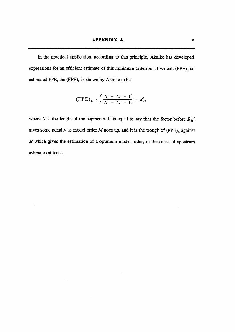
APPENDIX A c
In the practical application, according to this principle, Akaike has developed
expressions for an efficient estimate of this minimum criterion. If we call (FPE)e as
estimated FPE, the (FPE)e is shown by Akaike to be
< F P E > ' ■ ( % ! £ ! } ) • ^
where N is the length of the segments. It is equal to say that the factor before RM2
gives some penalty as model order M goes up, and it is the trough of (FPE)e against
M which gives the estimation of a optimum model order, in the sense of spectrum
estimates at least.

APPENDIX B
Details of the EEG signals used
The EEG data and the hypnograms of the first group records (subject 1 and 2)
used were kindly provided by Dr. S.J. Roberts of Oxford University. The EEG data
were obtained from healthy volunteers with no history of sleep disorders and
recorded on analogue cassette tape recorder (Medilog 9000-11 recorder, Oxford
Medical Ltd, Oxford.). The analogue bandwidth of the recorder is 0.5 - 40 Hz with
roll-of at -40 dB/decade. The EEG data was digitalized in 8 bit (0 - 255) with
sampling rate of 128 Hz and a low-pass digital filter of linear-phase was used with
the passband cut-off frequency of 30 Hz, a passband gain of 1±0.01 and a stopband
gain of -50 dB at 50 Hz.
The second group of records (e.i., subjects 3, 4, 5 and 6) were kindly supplied
by Dr. Chris Idzikowski (NCE Brainwaves, N. Ireland). The EEG signals were
obtained from healthy subjects with no history of sleep disorders and recorded on an
analogue recorder (Store 14 DS, Racal Recorders,). The EEG signals were
digitalized in 12 bit resolution with 122 Hz sampling rate and digitally filtered with

APPENDIX B b
a bandpass filter. The centre frequency of the filter is 17.8 Hz with bandwidth of
34.4 Hz and stopband attenuation of -50 dB. Left transition band was set to 0.3 Hz
and the right was set to 5 Hz.