Model-Based Clustering and Classification of Functional Data · approaches for model-based clustering and classification of functional data. We present well-grounded statistical models

ADVANCED REV I EW

Model-based clustering and classification of functional data

Faicel Chamroukhi1 | Hien D. Nguyen2

1Department of Mathematics and ComputerScience, Normandie University, UNICAEN, UMRCNRS LMNO, Caen, France2Department of Mathematics and Statistics, LaTrobe University, Melbourne, Victoria, Australia

CorrespondenceFaicel Chamroukhi, Department of Mathematicsand Computer Science, Normandie University,UNICAEN, UMR CNRS LMNO, 14000 Caen,France.Email: [email protected]

Funding informationAustralian Research Council, Grant/AwardNumbers: DP180101192, DE170101134; RégionNormandie, Grant/Award Number: RINAStERiCs; ANR, Grant/Award Number: SMILESANR-18-CE40-0014

Complex data analysis is a central topic of modern statistics and learning systemswhich is becoming of broader interest with the increasing prevalence of high-dimensional data. The challenge is to develop statistical models and autonomousalgorithms that are able to discern knowledge from raw data, which can beachieved through clustering techniques, or to make predictions of future data viaclassification techniques. Latent data models, including mixture model-basedapproaches, are among the most popular and successful approaches in both super-vised and unsupervised learning. Although being traditional tools in multivariateanalysis, they are growing in popularity when considered in the framework of func-tional data analysis (FDA). FDA is the data analysis paradigm in which each datumis a function, rather than a real vector. In many areas of application, including sig-nal and image processing, functional imaging, bioinformatics, etc., the analyzeddata are indeed often available in the form of discretized values of functions,curves, or surfaces. This functional aspect of the data adds additional difficultieswhen compared to classical multivariate data analysis. We review and presentapproaches for model-based clustering and classification of functional data. Wepresent well-grounded statistical models along with efficient algorithmic tools toaddress problems regarding the clustering and the classification of these functionaldata, including their heterogeneity, missing information, and dynamical hiddenstructures. The presented models and algorithms are illustrated via real-world func-tional data analysis problems from several areas of application.

This article is categorized under:Fundamental Concepts of Data and Knowledge > Data ConceptsAlgorithmic Development > StatisticsTechnologies > Statistical FundamentalsTechnologies > Structure Discovery and Clustering

KEYWORDS

algorithms, classification, clustering, EM, functional data analysis, mixturemodels

1 | INTRODUCTION

Complex data analysis is a central topic of modern statistics and statistical learning systems of broader interest, from both amethodological and a practical points of view, in particular within the big data context. The objective is to develop well-grounded statistical models and efficient algorithms that aim at discerning knowledge from raw data, while addressing prob-lems regarding the data complexity, including heterogeneity, high dimensionality, dynamical behaviors, and missing informa-tion. We can distinguish methods for exploratory analysis, which rely on clustering and segmentation techniques, and

Received: 3 April 2018 Revised: 17 November 2018 Accepted: 9 December 2018

DOI: 10.1002/widm.1298

WIREs Data Mining Knowl Discov. 2019;e1298. wires.wiley.com/dmkd © 2019 Wiley Periodicals, Inc. 1 of 36https://doi.org/10.1002/widm.1298

https://orcid.org/0000-0002-5894-3103

https://orcid.org/0000-0002-9958-432X

http://wires.wiley.com/dmkd

https://doi.org/10.1002/widm.1298

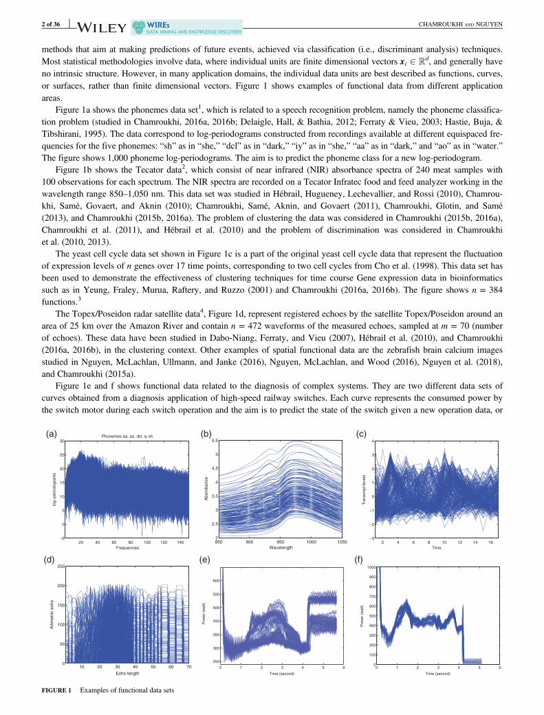
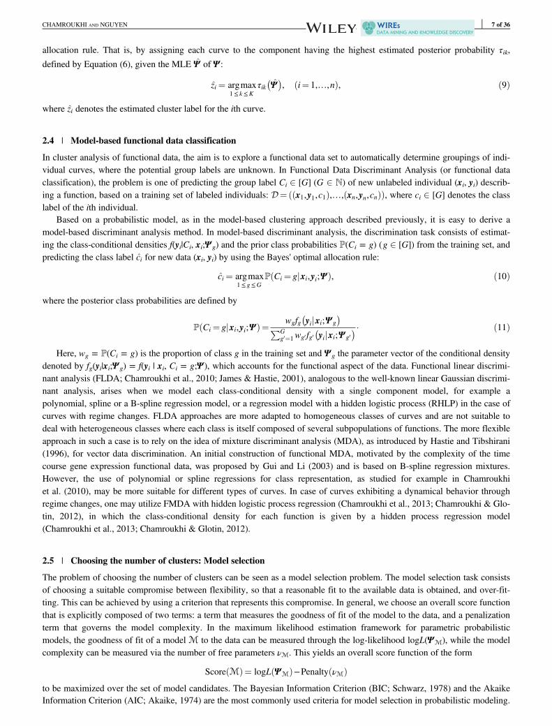
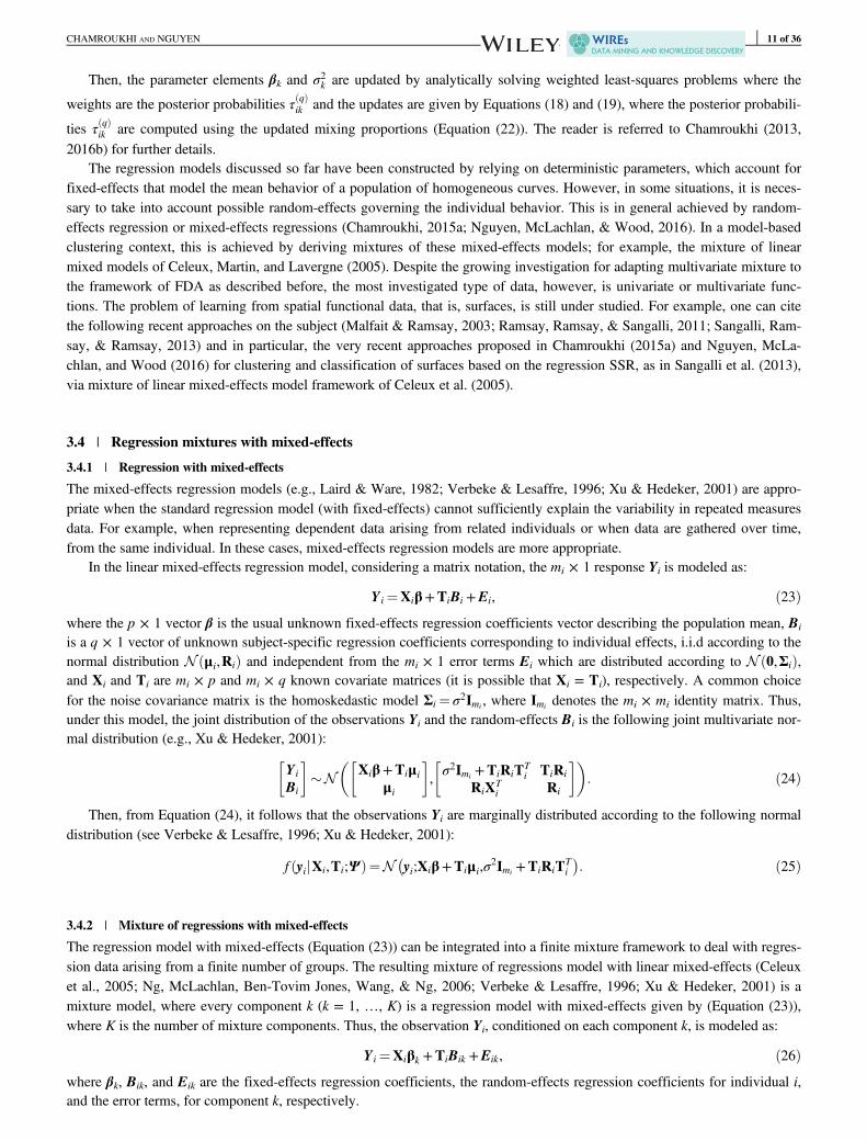
methods that aim at making predictions of future events, achieved via classification (i.e., discriminant analysis) techniques.Most statistical methodologies involve data, where individual units are finite dimensional vectors xi 2 Rd, and generally haveno intrinsic structure. However, in many application domains, the individual data units are best described as functions, curves,or surfaces, rather than finite dimensional vectors. Figure 1 shows examples of functional data from different applicationareas.

Figure 1a shows the phonemes data set1, which is related to a speech recognition problem, namely the phoneme classifica-tion problem (studied in Chamroukhi, 2016a, 2016b; Delaigle, Hall, & Bathia, 2012; Ferraty & Vieu, 2003; Hastie, Buja, &Tibshirani, 1995). The data correspond to log-periodograms constructed from recordings available at different equispaced fre-quencies for the five phonemes: “sh” as in “she,” “dcl” as in “dark,” “iy” as in “she,” “aa” as in “dark,” and “ao” as in “water.”The figure shows 1,000 phoneme log-periodograms. The aim is to predict the phoneme class for a new log-periodogram.

Figure 1b shows the Tecator data2, which consist of near infrared (NIR) absorbance spectra of 240 meat samples with100 observations for each spectrum. The NIR spectra are recorded on a Tecator Infratec food and feed analyzer working in thewavelength range 850–1,050 nm. This data set was studied in Hébrail, Hugueney, Lechevallier, and Rossi (2010), Chamrou-khi, Samé, Govaert, and Aknin (2010); Chamroukhi, Samé, Aknin, and Govaert (2011), Chamroukhi, Glotin, and Samé(2013), and Chamroukhi (2015b, 2016a). The problem of clustering the data was considered in Chamroukhi (2015b, 2016a),Chamroukhi et al. (2011), and Hébrail et al. (2010) and the problem of discrimination was considered in Chamroukhiet al. (2010, 2013).

The yeast cell cycle data set shown in Figure 1c is a part of the original yeast cell cycle data that represent the fluctuationof expression levels of n genes over 17 time points, corresponding to two cell cycles from Cho et al. (1998). This data set hasbeen used to demonstrate the effectiveness of clustering techniques for time course Gene expression data in bioinformaticssuch as in Yeung, Fraley, Murua, Raftery, and Ruzzo (2001) and Chamroukhi (2016a, 2016b). The figure shows n = 384functions.3

The Topex/Poseidon radar satellite data4, Figure 1d, represent registered echoes by the satellite Topex/Poseidon around anarea of 25 km over the Amazon River and contain n = 472 waveforms of the measured echoes, sampled at m = 70 (numberof echoes). These data have been studied in Dabo-Niang, Ferraty, and Vieu (2007), Hébrail et al. (2010), and Chamroukhi(2016a, 2016b), in the clustering context. Other examples of spatial functional data are the zebrafish brain calcium imagesstudied in Nguyen, McLachlan, Ullmann, and Janke (2016), Nguyen, McLachlan, and Wood (2016), Nguyen et al. (2018),and Chamroukhi (2015a).

Figure 1e and f shows functional data related to the diagnosis of complex systems. They are two different data sets ofcurves obtained from a diagnosis application of high-speed railway switches. Each curve represents the consumed power bythe switch motor during each switch operation and the aim is to predict the state of the switch given a new operation data, or

20 40 60 80 100 120 140−5

0

5

10

15

20

25

30

Frequencies

log

−p

erio

do

gra

ms

Phonemes aa, ao, dcl, iy sh

850 900 950 1000 10502

2.5

3

3.5

4

4.5

5

5.5

Wavelength

Ab

sro

ba

nce

2 4 6 8 10 12 14 16−3

−2

−1

0

1

2

3

4

Tra

nscrip

t le

ve

ls

Time

(a) (b) (c)

10 20 30 40 50 60 700

50

100

150

200

250

Echo length

Altim

etr

ic e

ch

o

0 1 2 3 4 5 60

100

200

300

400

500

600

700

800

900

1000

Time (second)

0 1 2 3 4 5 6

Time (second)

Po

we

r (w

att

)

250

600

550

500

450

350

300

Po

we

r (w

att

)

(d) (e) (f)

FIGURE 1 Examples of functional data sets

2 of 36 CHAMROUKHI AND NGUYEN

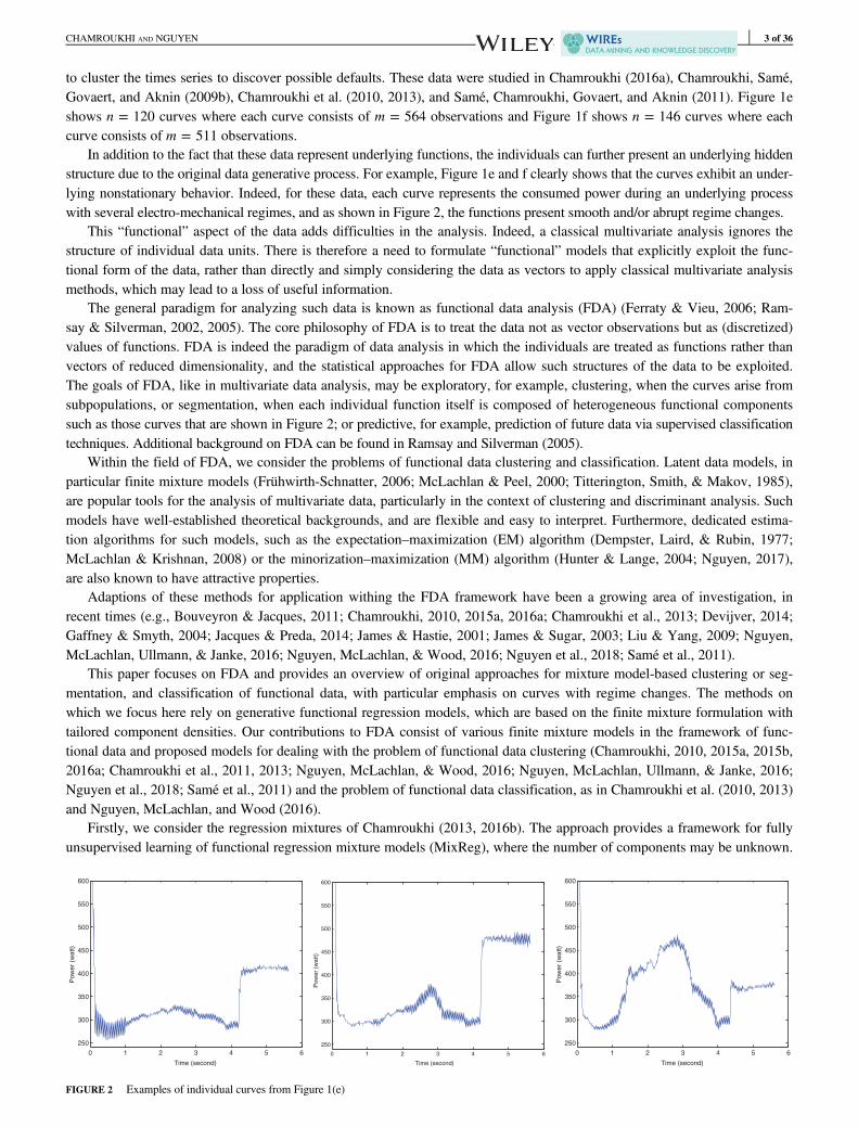
to cluster the times series to discover possible defaults. These data were studied in Chamroukhi (2016a), Chamroukhi, Samé,Govaert, and Aknin (2009b), Chamroukhi et al. (2010, 2013), and Samé, Chamroukhi, Govaert, and Aknin (2011). Figure 1eshows n = 120 curves where each curve consists of m = 564 observations and Figure 1f shows n = 146 curves where eachcurve consists of m = 511 observations.

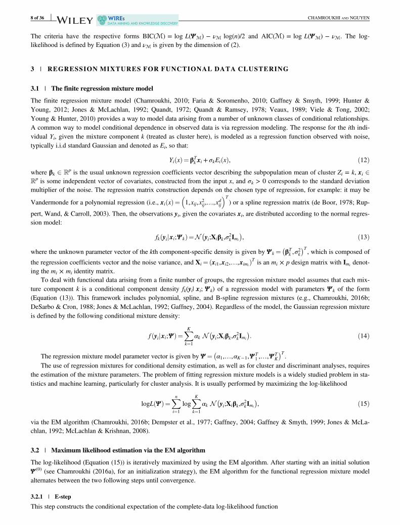
In addition to the fact that these data represent underlying functions, the individuals can further present an underlying hiddenstructure due to the original data generative process. For example, Figure 1e and f clearly shows that the curves exhibit an under-lying nonstationary behavior. Indeed, for these data, each curve represents the consumed power during an underlying processwith several electro-mechanical regimes, and as shown in Figure 2, the functions present smooth and/or abrupt regime changes.

This “functional” aspect of the data adds difficulties in the analysis. Indeed, a classical multivariate analysis ignores thestructure of individual data units. There is therefore a need to formulate “functional” models that explicitly exploit the func-tional form of the data, rather than directly and simply considering the data as vectors to apply classical multivariate analysismethods, which may lead to a loss of useful information.

The general paradigm for analyzing such data is known as functional data analysis (FDA) (Ferraty & Vieu, 2006; Ram-say & Silverman, 2002, 2005). The core philosophy of FDA is to treat the data not as vector observations but as (discretized)values of functions. FDA is indeed the paradigm of data analysis in which the individuals are treated as functions rather thanvectors of reduced dimensionality, and the statistical approaches for FDA allow such structures of the data to be exploited.The goals of FDA, like in multivariate data analysis, may be exploratory, for example, clustering, when the curves arise fromsubpopulations, or segmentation, when each individual function itself is composed of heterogeneous functional componentssuch as those curves that are shown in Figure 2; or predictive, for example, prediction of future data via supervised classificationtechniques. Additional background on FDA can be found in Ramsay and Silverman (2005).

Within the field of FDA, we consider the problems of functional data clustering and classification. Latent data models, inparticular finite mixture models (Frühwirth-Schnatter, 2006; McLachlan & Peel, 2000; Titterington, Smith, & Makov, 1985),are popular tools for the analysis of multivariate data, particularly in the context of clustering and discriminant analysis. Suchmodels have well-established theoretical backgrounds, and are flexible and easy to interpret. Furthermore, dedicated estima-tion algorithms for such models, such as the expectation–maximization (EM) algorithm (Dempster, Laird, & Rubin, 1977;McLachlan & Krishnan, 2008) or the minorization–maximization (MM) algorithm (Hunter & Lange, 2004; Nguyen, 2017),are also known to have attractive properties.

Adaptions of these methods for application withing the FDA framework have been a growing area of investigation, inrecent times (e.g., Bouveyron & Jacques, 2011; Chamroukhi, 2010, 2015a, 2016a; Chamroukhi et al., 2013; Devijver, 2014;Gaffney & Smyth, 2004; Jacques & Preda, 2014; James & Hastie, 2001; James & Sugar, 2003; Liu & Yang, 2009; Nguyen,McLachlan, Ullmann, & Janke, 2016; Nguyen, McLachlan, & Wood, 2016; Nguyen et al., 2018; Samé et al., 2011).

This paper focuses on FDA and provides an overview of original approaches for mixture model-based clustering or seg-mentation, and classification of functional data, with particular emphasis on curves with regime changes. The methods onwhich we focus here rely on generative functional regression models, which are based on the finite mixture formulation withtailored component densities. Our contributions to FDA consist of various finite mixture models in the framework of func-tional data and proposed models for dealing with the problem of functional data clustering (Chamroukhi, 2010, 2015a, 2015b,2016a; Chamroukhi et al., 2011, 2013; Nguyen, McLachlan, & Wood, 2016; Nguyen, McLachlan, Ullmann, & Janke, 2016;Nguyen et al., 2018; Samé et al., 2011) and the problem of functional data classification, as in Chamroukhi et al. (2010, 2013)and Nguyen, McLachlan, and Wood (2016).

Firstly, we consider the regression mixtures of Chamroukhi (2013, 2016b). The approach provides a framework for fullyunsupervised learning of functional regression mixture models (MixReg), where the number of components may be unknown.

0 1 2 3 4 5 6

250

300

350

400

450

500

550

600

Time (second)

Pow

er

(watt)

0 1 2 3 4 5 6

250

300

350

400

450

500

550

600

Time (second)

Po

we

r (w

att

)

0 1 2 3 4 5 6

250

300

350

400

450

500

550

600

Time (second)

Pow

er

(watt)

FIGURE 2 Examples of individual curves from Figure 1(e)

CHAMROUKHI AND NGUYEN 3 of 36

The developed approach consists of a penalized maximum likelihood estimation problem that can be solved by a robust EM-like algorithm. Polynomial, spline, and B-spline versions of the approach are described.

Secondly, we consider the mixed-effects regression framework for FDA of Nguyen, McLachlan, and Wood (2016) andChamroukhi (2015a). In particular, we consider the application of such a framework for clustering spatial functional data. Weintroduce both the spatial spline regression (SSR) model with mixed-effects and the Bayesian SSR (BSSR) for modeling spa-tial function data. The SSR models are based on nodal basis functions (NBF) for spatial regression and accommodate bothcommon mean behavior for the data through a fixed-effects component, and interindividual variability via a random-effectscomponent. Then, in order to model populations of spatial functional data sampled from heterogeneous groups, we introducemixtures of SSRs with mixed-effects (MSSR) and Bayesian MSSR (BMSSR). Note that the term spatial in the presentedmodels only refers to data collected over a two-dimensional domain, with spatial dependence only implicitly accounted for viathe nature of the spline bases.

Thirdly, we consider the analysis of unlabeled functional data that might present a hidden longitudinal structure. More spe-cifically, we propose mixture-model based cluster and discriminant analyzes based on latent processes, to deal with functionaldata presenting smooth and/or abrupt regime changes. The heterogeneity of a population of functions arising in several sub-populations is naturally accommodated by a mixture distribution, and the dynamic behavior within each subpopulation, gener-ated by a nonstationary process typically governed by a regime change, is captured via a dedicated latent process. Here, thelatent process is modeled by either a Markov chain, a logistic process, or as a deterministic process with piecewise segments.We present a mixture model with piecewise regression mixture components (PWRM) for simultaneous clustering and segmen-tation of univariate regime changing functions (Chamroukhi, 2016a). Then, we formulate the problem from a fully generativeperspective by proposing the mixture of hidden Markov model regressions (MixHMMR) (Chamroukhi, 2015b; Chamroukhiet al., 2011) and the mixture of regressions with hidden logistic processes (MixRHLP) (Chamroukhi, 2010; Chamroukhiet al., 2013; Samé et al., 2011), which offers additional attractive features including the possibility to deal with smooth dynam-ics within the curves. We also present discriminant analyzes for homogeneous groups of functions (Chamroukhi et al., 2010),as well as for heterogeneous groups (Chamroukhi et al., 2013). The discriminant analysis is adapted for functions that mightbe organized in homogeneous or heterogeneous groups and further exhibit a nonstationary behavior due to regime changes.

The remainder of this paper is organized as follows. In Section 2, we present the general mixture modeling framework forfunctional data clustering and classification. Then, in Section 3, we present the regression mixture models for functional dataclustering, including the standard regression mixture, the regularized regression mixture, and the regression mixture with fixedand mixed-effects, which may be applied to both longitudinal and spatial data. We then present finite mixtures for simulta-neous functional data clustering and segmentation. Here, we consider three main models. The first is the PWRM model, pre-sented in Section 4.1. In Section 4.2, we then present the mixture of MixHMMR model. Section 4.3 is dedicated to themixture of regression models with hidden logistic processes (MixRHLP). Finally, in Section 5, we present some formulationsfor functional discriminant analysis, in particular, the functional mixture discriminant analysis (FMDA) with hidden processregression. The time complexities of the presented algorithms are discussed in Section 6. Numerous illustrative examples ofthe presented models and algorithms are provided throughout the article.

2 | MIXTURE MODELING FRAMEWORK FOR FUNCTIONAL DATA

Let (Y1(x), Y2(x), …, Yn(x)), x2T �R, be a random sample of n independently and identically distributed (i.i.d) functions,where Yi(x) is the response for the ith individual, given some input x, which can be the sampling time in a time series, or exog-enous covariates. The ith individual function (i = 1, …, n) is supposed to be observed at the independent abscissa valuesxi1,…,ximið Þ, with xij 2T for j = 1, …, mi and xi1 <…< ximi . The analyzed data are often available in the form of discretizedvalues of functions, curves (e.g., time series or waveforms), or surfaces (e.g., 2D-images or spatiotemporal data). Let D¼x1,y1ð Þ,…, xn,ynð Þð Þ be an observed sample of these functions, where each individual curve (xi, yi) consists of the mi responses

yi ¼ yi1,…,yimið Þ, over the covariate values xi1,…,ximið Þ.

2.1 | The functional mixture model

Consider the finite mixture modeling framework (Frühwirth-Schnatter, 2006; McLachlan & Peel, 2000; Titterington et al.,1985) for analysis of functional data. The finite mixture model decomposes the probability density of the observed data into aconvex sum of a finite number of component densities. The mixture model for functional data, which will be referred tohenceforth as the “functional mixture model,” has components that are dedicated to functional data modeling. It assumes thatthe observed pairs (x, y) are generated from K 2 N (where K is possibly unknown) functional probability density components,and are governed by a hidden categorical random variable Z 2 [K] = {1, …, K} that indicates the component from which a


particular observed pair is drawn. Thus, the functional mixture model can be defined by the following parametric densityfunction:

f yijxi;Ψð Þ¼XKk¼1

αkfk yi j xi;Ψ kð Þ� ð1Þ

The functional mixture model is parameterized by the parameter vector Ψ 2RνΨ (νΨ 2 N), defined by

Ψ ¼ α1,…,αK−1,Ψ T1 ,…,Ψ T

K

� �T, ð2Þ

where the αks, defined by αk = P(Zi = k), are the mixing proportions such that αk > 0 for each k andPK

k¼1αk ¼ 1, and Ψ k

(k = 1, …, K) is the parameter vector of the kth component density. In mixture modeling for FDA, each of the componentdensities fk(yi | xi;Ψ k), which denotes f(yi | x, Zi = k;Ψ ), can be chosen to adequately represent the functions for each group k.

Finite mixture models have been thoroughly studied in the multivariate analysis literature. There has been a strong empha-sis on incorporating aspects of functional data analytics into the construction of such models. The resulting models are betterable to handle functional data structures than vector-valued mixture models, and are referred to as functional mixture models(e.g., Chamroukhi, 2010, 2015a, 2016a; Chamroukhi et al., 2009b, 2010, 2013; Devijver, 2014; Gaffney, 2004; Gaffney &Smyth, 1999, 2004; Jacques & Preda, 2014; James & Hastie, 2001; James & Sugar, 2003; Liu & Yang, 2009; Nguyen, McLa-chlan, & Wood, 2016; Nguyen, McLachlan, Ullmann, & Janke, 2016; Samé et al., 2011). In the case of model-based curveclustering, there are a variety of modeling approaches such as the regression mixture approaches (Gaffney, 2004; Gaffney &Smyth, 1999), including polynomial regression, spline regression, and random-effects polynomial regression, as in Gaffneyand Smyth (2004), or B-spline regression as in Liu and Yang (2009).

When clustering sparsely sampled curves, one may use the mixture approach based on splines as in James and Sugar(2003). In Devijver (2014) and Giacofci, Lambert-Lacroix, Marot, and Picard (2013), the clustering is performed by filteringthe data via a wavelet basis instead of a B-spline basis. Another alternative, which concerns mixture model-based clustering ofmultivariate functional data, is that in which the clustering is performed in the space of reduced functional principal compo-nents (Jacques & Preda, 2014). Other alternatives are the K-means-based clustering of functional data by using B-spline bases(Abraham, Cornillon, Matzner-Lober, & Molinari, 2003) or wavelet bases as in Antoniadis, Brossat, Cugliari, and Poggi(2013). Autoregressive moving average mixtures have also been considered in Xiong and Yeung (2004) for time series clus-tering. Beyond these (semi-)parametric approaches, one can also find nonparametric statistical methods (Ferraty & Vieu,2003) using kernel density estimators (Delaigle et al., 2012), using mixture of Gaussian processes regression (Shi & Choi,2011; Shi, Murray-Smith, & Titterington, 2005; Shi & Wang, 2008), or using hierarchical Gaussian process mixtures forregression (Shi et al., 2005; Shi & Choi, 2011).

In functional data discrimination, the generative approaches for functional data related to this work are essentially basedon functional linear discriminant analysis using splines, including B-splines as in James and Hastie (2001), or are based onMDA (Hastie & Tibshirani, 1996) in the context of functional data, by relying on B-spline bases (Gui & Li, 2003). Delaigleet al. (2012) have also addressed the functional data discrimination problem from a nonparametric perspective using a kernel-based method.

2.2 | Maximum likelihood estimation framework via the EM algorithm

The parameter vector Ψ of the FunMM (1) can be estimated by maximizing the observed data log-likelihood thanks to thedesirable asymptotic properties of the maximum likelihood estimator (MLE), and the effectiveness of the available algorithmictools to compute such estimators, such as the EM algorithm. Given an i.i.d sample of n observed functionsD¼ x1,y1ð Þ,…, xn,ynð Þð Þ, the log-likelihood of Ψ , given the observed data D, is given by:

logL Ψð Þ¼Xni¼1

logXKk¼1

αkfk yijxi;Ψ kð Þ: ð3Þ

The maximization of this log-likelihood cannot be performed in a closed form. By using the EM algorithm, we can obtaina root of Equation (3). The EM algorithm (Dempster et al., 1977; McLachlan & Krishnan, 2008) or its extensions have manydesirable properties including stability and convergence guarantees (see Dempster et al., 1977; McLachlan & Krishnan, 2008for more details), and can be used to iteratively maximize the log-likelihood function. The EM algorithm for the maximizationof Equation (3) firstly requires the construction of the complete-data log-likelihood


logLc Ψð Þ¼Xni¼1

XKk¼1

Zik log αkfk yijxi;Ψ kð Þ½ �, ð4Þ

where Zik is an indicator binary-valued variable such that Zik = 1 if Zi = k (i.e., if the ith curve (xi, yi) is generated from thekth mixture component) and Zik = 0 otherwise. Thus, the EM algorithm for the FunMM, in its general form, runs as follows.After starting with an initial solution Ψ (0), the EM algorithm for the functional mixture model alternates between the two fol-lowing steps, until convergence (e.g., when there is no longer a significant change in the values of the log-likelihood). Thereare a number of ways in which the initial solution Ψ (0) can be obtained. The simplest of which, as suggested in McLachlanand Peel (2000), is to randomly partition the data and to utilize this partitioning to compute an initial solution. When appropri-ate, a pair of alternative methods is to utilize the K-means algorithm or a hierarchical clustering algorithm in order to obtain aninitial partition, and thus an initial solution for Ψ . These solutions are implemented in the popular software packages Emmixs-kew of Wang, Ng, and McLachlan (2009) and mclust of Scrucca, Fop, Murphy, and Raftery (2016). For the specific mixturemodels presented here, initialization strategies are provided and implemented in Chamroukhi (2010, 2016a), Chamroukhiet al. (2011), and Samé et al. (2011).

2.2.1 | E-step

This step computes the expectation of the complete-data log-likelihood (Equation (4)), given the observed data D, using thecurrent parameter vector Ψ (q):

Q Ψ ;Ψ qð Þ� �

¼E logLc Ψð ÞjD;Ψ qð Þh i

¼Xni¼1

XKk¼1

τ qð Þik log αkfk yijxi;Ψ kð Þ½ �, ð5Þ

where

τ qð Þik ¼P Zi ¼ kjyi,xi;Ψ qð Þ

� �¼α qð Þk fk yijxi;Ψ

qð Þk

� �f yijxi;Ψ qð Þ� � , ð6Þ

is the posterior probability that the curve (xi, yi) is generated by the kth cluster. This step therefore only requires the computa-

tion of the posterior probabilities of component membership τ qð Þik (i = 1, …, n), for each of the K components.

2.2.2 | M-step

This step updates the value of the parameter vector Ψ by maximizing the Q-function (Equation (5)) with respect to (w.r.t) Ψ ,that is, by computing the parameter vector update

Ψ q+1ð Þ ¼ argmaxΨ


: ð7Þ

The updates of the mixing proportions correspond to those of the standard mixture model:

α q+1ð Þk ¼ 1

n

Xni¼1

τ qð Þik , ð8Þ

while the mixture components parameters' updates Ψ q+1ð Þk depend on the chosen functional mixture components fk(yi|xi;Ψ k).

The EM algorithm monotonically increases the log-likelihood (Dempster et al., 1977; McLachlan & Krishnan, 2008). Fur-thermore, the sequence of parameter estimates generated by the EM algorithm converges toward a local maximum of the log-likelihood function (Wu, 1983). The EM algorithm has a number of advantages, including its numerical stability, simplicity ofimplementation, and reliable convergence. In addition, by using adapted initialization, one may attempt to globally maximizethe log-likelihood function.

In general, both the E- and M-steps have simple forms when the complete-data probability density function is from theexponential family (McLachlan & Krishnan, 2008). Some of the drawbacks of the EM algorithm are that it is sometimes slowto converge, and in some problems, the E- or M-step may be analytically intractable. Fortunately, there exist extensions of theEM framework that can tackle these problems (McLachlan & Krishnan, 2008).

2.3 | Model-based functional data clustering

Once the model parameters have been estimated, a soft partition of the data into K clusters, represented by the estimated poste-

rior probabilities τik ¼P Zi ¼ kjxi,yi; Ψ� �

, is obtained. A hard partition can also be computed according to the Bayes' optimal


allocation rule. That is, by assigning each curve to the component having the highest estimated posterior probability τik,

defined by Equation (6), given the MLE Ψ of Ψ :

zi ¼ argmax1≤ k≤K

τik Ψ� �

, i¼ 1,…,nð Þ, ð9Þ

where zi denotes the estimated cluster label for the ith curve.

2.4 | Model-based functional data classification

In cluster analysis of functional data, the aim is to explore a functional data set to automatically determine groupings of indi-vidual curves, where the potential group labels are unknown. In Functional Data Discriminant Analysis (or functional dataclassification), the problem is one of predicting the group label Ci 2 [G] (G 2 N) of new unlabeled individual (xi, yi) describ-ing a function, based on a training set of labeled individuals: D¼ x1,y1,c1ð Þ,…, xn,yn,cnð Þð Þ, where ci 2 [G] denotes the classlabel of the ith individual.

Based on a probabilistic model, as in the model-based clustering approach described previously, it is easy to derive amodel-based discriminant analysis method. In model-based discriminant analysis, the discrimination task consists of estimat-ing the class-conditional densities f(yi|Ci, xi;Ψ g) and the prior class probabilities P(Ci = g) (g 2 [G]) from the training set, andpredicting the class label ci for new data (xi, yi) by using the Bayes' optimal allocation rule:

ci ¼ argmax1≤ g≤G

P Ci ¼ gjxi,yi;Ψð Þ, ð10Þ

where the posterior class probabilities are defined by

P Ci ¼ gjxi,yi;Ψð Þ¼wgfg yijxi;Ψ g

� �PG

g0¼1wg0 fg0 yijxi;Ψ g0� � � ð11Þ

Here, wg = P(Ci = g) is the proportion of class g in the training set and Ψ g the parameter vector of the conditional densitydenoted by fg(yi|xi;Ψ g) = f(yi | xi, Ci = g;Ψ ), which accounts for the functional aspect of the data. Functional linear discrimi-nant analysis (FLDA; Chamroukhi et al., 2010; James & Hastie, 2001), analogous to the well-known linear Gaussian discrimi-nant analysis, arises when we model each class-conditional density with a single component model, for example apolynomial, spline or a B-spline regression model, or a regression model with a hidden logistic process (RHLP) in the case ofcurves with regime changes. FLDA approaches are more adapted to homogeneous classes of curves and are not suitable todeal with heterogeneous classes where each class is itself composed of several subpopulations of functions. The more flexibleapproach in such a case is to rely on the idea of mixture discriminant analysis (MDA), as introduced by Hastie and Tibshirani(1996), for vector data discrimination. An initial construction of functional MDA, motivated by the complexity of the timecourse gene expression functional data, was proposed by Gui and Li (2003) and is based on B-spline regression mixtures.However, the use of polynomial or spline regressions for class representation, as studied for example in Chamroukhiet al. (2010), may be more suitable for different types of curves. In case of curves exhibiting a dynamical behavior throughregime changes, one may utilize FMDA with hidden logistic process regression (Chamroukhi et al., 2013; Chamroukhi & Glo-tin, 2012), in which the class-conditional density for each function is given by a hidden process regression model(Chamroukhi et al., 2013; Chamroukhi & Glotin, 2012).

2.5 | Choosing the number of clusters: Model selection

The problem of choosing the number of clusters can be seen as a model selection problem. The model selection task consistsof choosing a suitable compromise between flexibility, so that a reasonable fit to the available data is obtained, and over-fit-ting. This can be achieved by using a criterion that represents this compromise. In general, we choose an overall score functionthat is explicitly composed of two terms: a term that measures the goodness of fit of the model to the data, and a penalizationterm that governs the model complexity. In the maximum likelihood estimation framework for parametric probabilisticmodels, the goodness of fit of a model ℳ to the data can be measured through the log-likelihood logL(Ψℳ), while the modelcomplexity can be measured via the number of free parameters νℳ. This yields an overall score function of the form

Score ℳð Þ¼ logL Ψℳð Þ−Penalty νℳð Þ

to be maximized over the set of model candidates. The Bayesian Information Criterion (BIC; Schwarz, 1978) and the AkaikeInformation Criterion (AIC; Akaike, 1974) are the most commonly used criteria for model selection in probabilistic modeling.


The criteria have the respective forms BIC(ℳ) = log L(Ψℳ) − νℳ log(n)/2 and AIC(ℳ) = log L(Ψℳ) − νℳ. The log-likelihood is defined by Equation (3) and νℳ is given by the dimension of (2).

3 | REGRESSION MIXTURES FOR FUNCTIONAL DATA CLUSTERING

3.1 | The finite regression mixture model

The finite regression mixture model (Chamroukhi, 2010; Faria & Soromenho, 2010; Gaffney & Smyth, 1999; Hunter &Young, 2012; Jones & McLachlan, 1992; Quandt, 1972; Quandt & Ramsey, 1978; Veaux, 1989; Viele & Tong, 2002;Young & Hunter, 2010) provides a way to model data arising from a number of unknown classes of conditional relationships.A common way to model conditional dependence in observed data is via regression modeling. The response for the ith indi-vidual Yi, given the mixture component k (treated as cluster here), is modeled as a regression function observed with noise,typically i.i.d standard Gaussian and denoted as Ei, so that:

Yi xð Þ¼βTk xi + σkEi xð Þ, ð12Þ

where βk 2 Rp is the usual unknown regression coefficients vector describing the subpopulation mean of cluster Zi = k, xi 2Rp is some independent vector of covariates, constructed from the input x, and σk > 0 corresponds to the standard deviationmultiplier of the noise. The regression matrix construction depends on the chosen type of regression, for example: it may be

Vandermonde for a polynomial regression (i.e., xi xð Þ¼ 1,xij,x2ij,…,xdij� �T

) or a spline regression matrix (de Boor, 1978; Rup-

pert, Wand, & Carroll, 2003). Then, the observations yi, given the covariates xi, are distributed according to the normal regres-sion model:

fk yijxi;Ψ kð Þ¼N yi;Xiβk,σ2kImi

� �, ð13Þ

where the unknown parameter vector of the kth component-specific density is given by Ψ k ¼ βTk ,σ

2k

� �T, which is composed of

the regression coefficients vector and the noise variance, and Xi ¼ xi1,xi2,…,ximið ÞT is an mi × p design matrix with Imi denot-ing the mi × mi identity matrix.

To deal with functional data arising from a finite number of groups, the regression mixture model assumes that each mix-ture component k is a conditional component density fk(yi| xi; Ψ k) of a regression model with parameters Ψ k of the form(Equation (13)). This framework includes polynomial, spline, and B-spline regression mixtures (e.g., Chamroukhi, 2016b;DeSarbo & Cron, 1988; Jones & McLachlan, 1992; Gaffney, 2004). Regardless of the model, the Gaussian regression mixtureis defined by the following conditional mixture density:


αk N yi;Xiβk,σ2kImi

� �: ð14Þ

The regression mixture model parameter vector is given by Ψ ¼ α1,…,αK−1,Ψ T1 ,…,Ψ T

K

� �T.

The use of regression mixtures for conditional density estimation, as well as for cluster and discriminant analyses, requiresthe estimation of the mixture parameters. The problem of fitting regression mixture models is a widely studied problem in sta-tistics and machine learning, particularly for cluster analysis. It is usually performed by maximizing the log-likelihood


logXKk¼1

αk N yi;Xiβk,σ2kImi

� �, ð15Þ

via the EM algorithm (Chamroukhi, 2016b; Dempster et al., 1977; Gaffney, 2004; Gaffney & Smyth, 1999; Jones & McLa-chlan, 1992; McLachlan & Krishnan, 2008).

3.2 | Maximum likelihood estimation via the EM algorithm

The log-likelihood (Equation (15)) is iteratively maximized by using the EM algorithm. After starting with an initial solutionΨ (0) (see Chamroukhi (2016a), for an initialization strategy), the EM algorithm for the functional regression mixture modelalternates between the two following steps until convergence.

3.2.1 | E-step

This step constructs the conditional expectation of the complete-data log-likelihood function



¼Xni¼1

XKk¼1

τ qð Þik log αkN yi;Xiβk,σ2kImi

� �� , ð16Þ

which only requires computing the posterior probabilities of component membership τ qð Þik (i = 1, …, n) for each of the

K components. That is, the posterior probability that the curve (xi, yi) is generated by the kth cluster, as defined inEquation (6):

τ qð Þik ¼ α qð Þ

k N yi;XiβT qð Þk ,σ2 qð Þ

k Imi

� �=XKh¼1

α qð Þh N yi;Xiβ qð Þ

h ,σ2 qð Þh Imi

� �: ð17Þ

3.2.2 | M-step

This step updates the value of the parameter vector Ψ by maximizing Equation (16) w.r.t Ψ . That is, by computing the param-eter vector update Ψ (q + 1), given by Equation (7). The mixing proportions updates are given by Equation (8). Then, theregression parameters are updated by maximizing Equation (16) w.r.t βk,σ2k

� �. This corresponds to analytically solving

K weighted least-squares problems, where the weights are the posterior probabilities τ qð Þik and the updates are given by:

β q+1ð Þk ¼

Xni¼1

τ qð Þik XT

i Xi

" #−1Xni¼1

τ qð Þik XT

i yi, ð18Þ

σ2 q+1ð Þk ¼ 1Pn

i¼1 τqð Þik mi

Xni¼1

τ qð Þik k yi−Xiβ q+1ð Þ

k k2: ð19Þ

Then, once the model parameters have been estimated, a soft partition of the data into K clusters, represented by the esti-mated posterior cluster probabilities τik, is obtained. A hard partition can also be computed according to the Bayes' optimalallocation rule (Equation (9)).

Selecting the number of mixture components can be addressed by using some model selection criteria (e.g., AIC or BIC asdiscussed in Section 2.5), to choose one model from a set of preestimated candidate models.

In the next section, we revisit these functional mixture models and their estimation from another prospective by consider-ing regularized MLE rather than standard MLE. This particularly attempts to address the issue of initialization, and allows formodel selection via regularization. Indeed, it is well-known that care is required when initializing any EM algorithm. The EMalgorithm also requires the number of mixture component to be given a priori. Here we propose a penalized MLE approach,carried out via a robust EM-like algorithm, which simultaneously infers the model parameters, the model structure and the par-tition (Chamroukhi, 2013, 2016b), and in which the initialization is simple. This results in a fully unsupervised algorithm forfitting regression mixtures.

3.3 | Regularized regression mixtures for functional data

It is well-known that care is required when initializing any EM algorithm. If the initialization is not carefully performed, thenthe EM algorithm may lead to unsatisfactory results (See for example Biernacki, Celeux, & Govaert, 2003; Reddy, Chiang, &Rajaratnam, 2008; Yang, Lai, & Lin, 2012 for discussions). Thus, fitting regression mixture models with the standard EMalgorithm may yield poor estimations if the model parameters are not initialized properly.

EM algorithm initialization in general can be performed via random partitioning of the data, or by computing a partitionfrom another clustering algorithm such as K-means, Classification EM (Celeux & Diebolt, 1985; McLachlan, 1982, CEM),Stochastic EM (Celeux & Govaert, 1992), etc, or by initializing the EM algorithm via randomization, followed by a numberof iterations of the EM algorithm, itself.

Several approaches have been proposed in the literature in order to overcome the initialization problem, and to make theEM algorithm for Gaussian mixture models robust to initialization (e.g., Biernacki et al., 2003; Reddy et al., 2008; Yanget al., 2012). Further details about choosing starting values for the EM algorithm for Gaussian mixtures can be found in Bier-nacki et al. (2003). In addition to sensitivity regarding the initialization, the EM algorithm requires the number of mixturecomponents to be known. Some authors have considered alternative approaches in order to estimate the unknown number ofmixture components in Gaussian mixture models, for example by an adapted EM algorithm such as in Figueiredo and Jain(2000) and Yang et al. (2012), or from a Bayesian prospective (Richardson & Green, 1997), by reversible jump Markov ChainMonte Carlo (MCMC). However, in general, these two issues have been considered separately.


Among the approaches that consider the problem of robustness with regard to initial values and estimating the number ofmixture components, in the same algorithm, there is the EM algorithm proposed by Figueiredo and Jain (2000). The aforemen-tioned EM algorithm is capable of selecting the number of components and attempts to reduce the sensitivity with regard toinitial values by optimizing a minimum message length criterion, which is a penalized log-likelihood. It starts by fitting a mix-ture model with a large number of components and discards invalid components as the learning proceeds.

The degree of validity of each component is measured through the penalization term, which includes the mixing propor-tions, to deduce whether the associated cluster is small or not, to be discarded. More recently, in Yang et al. (2012), theauthors developed a robust EM-like algorithm for model-based clustering of multivariate data using Gaussian mixture modelsthat simultaneously addresses the problem of initialization and estimation of the number of mixture components. That algo-rithm overcomes some initialization drawback of the EM algorithm proposed in Figueiredo and Jain (2000). As shown inYang et al. (2012), the problem regarding initialization is more serious for data with a large number of clusters.

However, these presented model-based clustering approaches, including those in Yang et al. (2012) and Figueiredo andJain (2000), are concerned with vector-valued data. When the data are curves or functions, such methods are not appropriate.The functional mixture models of form (Equation (1)), are better able to handle functional data structures. By using such func-tional mixture models, we can overcome the limitations of the EM algorithm for model-based functional data clustering byregularizing the estimation objective (Equation (15)).

The presented approach, as developed in Chamroukhi (2013, 2016b), is in the same spirit of the EM-like algorithm pre-sented in Yang et al. (2012), but extends the the idea to functional data clustering, rather than multivariate data clustering. Thisleads to a regularized estimation of the regression mixture models (including splines or B-splines) of form (Equation (14)),and the resulting EM-like algorithm is robust to initialization and automatically estimates the optimal number of clusters asthe learning proceeds.

Rather than maximizing the standard log-likelihood (Equation (15)), we presented, in Chamroukhi (2013, 2016b), a penal-ized log-likelihood function constructed by penalizing the log-likelihood by a regularization term related to the model com-plexity, defined by:

J λ,Ψð Þ¼ logL Ψð Þ−λH Zð Þ, λ≥ 0, ð20Þ

where logL(Ψ ) is the log-likelihood maximized by the standard EM algorithm for regression mixtures (see Equation (15)),λ ≥ 0 is a parameter that controls the complexity of the fitted model, and Z = (Z1, …, Zn). This penalized log-likelihood func-tion allows for the control of the complexity of the model fit, through the roughness penalty H(Z). As the model complexity isrelated to the number of mixture components and therefore the structure of the hidden variables Zi (recall that Zi represents theclass label of the ith curve), we chose to use the entropy of the hidden variable Zi as penalty. The framework of selecting thenumber of mixture components in model-based clustering by using an entropy-based regularization of the log-likelihood isdiscussed in Baudry (2015). The penalized log-likelihood criterion is as follows. The (differential) entropy of Zi is defined by:

H Zið Þ¼ −PK

k¼1P Zi ¼ kð Þ logP Zi ¼ kð Þ¼ −PK

k¼1αk logαk and the total entropy for Z is therefore additive and equates to

H Zð Þ¼ −Xni¼1

XKk¼1

αk logαk� ð21Þ

The penalized log-likelihood function (Equation (20)) allows for simultaneous control of the complexity of the model fit,through the roughness penalty λ H(Z). The entropy term H(Z) measures the complexity of a fitted model for K clusters. Whenthe entropy is large, the fitted model is rougher, and when it is small, the fitted model is smoother. The nonnegative smoothingparameter λ establishes a trade-off between closeness of fit to the data and the smoothness of fit. As λ increases, the fittedmodel tends to be less complex, and we get a smoother fit.

The proposed robust EM-like algorithm to maximize the penalized log-likelihood J λ,θð Þ for regression mixture densityestimation and model-based curve clustering appears in Chamroukhi (2013, 2016b). The E-step computes the posterior proba-bilities of component membership according to Equation (17). Then, the M-step updates the value of the parameter vector Ψ .The mixing proportions updates are given by (e.g., Appendix B in Chamroukhi, 2016b, for details):

α q+1ð Þk ¼ 1

n

Xni¼1

τ qð Þik + λα qð Þ

k logα qð Þk −

XKh¼1

α qð Þh logα qð Þ

h

!� ð22Þ

We remark here that the update of the mixing proportions (Equation (22)) is close to the standard EM algorithm update fora mixture model (Equation (8)) for very small value of λ. However, for a large value of λ, the penalization term will play a rolein penalizing small clusters and thus allows for the reduction of complexity.


Then, the parameter elements βk and σ2k are updated by analytically solving weighted least-squares problems where the

weights are the posterior probabilities τ qð Þik and the updates are given by Equations (18) and (19), where the posterior probabili-

ties τ qð Þik are computed using the updated mixing proportions (Equation (22)). The reader is referred to Chamroukhi (2013,

2016b) for further details.The regression models discussed so far have been constructed by relying on deterministic parameters, which account for

fixed-effects that model the mean behavior of a population of homogeneous curves. However, in some situations, it is neces-sary to take into account possible random-effects governing the individual behavior. This is in general achieved by random-effects regression or mixed-effects regressions (Chamroukhi, 2015a; Nguyen, McLachlan, & Wood, 2016). In a model-basedclustering context, this is achieved by deriving mixtures of these mixed-effects models; for example, the mixture of linearmixed models of Celeux, Martin, and Lavergne (2005). Despite the growing investigation for adapting multivariate mixture tothe framework of FDA as described before, the most investigated type of data, however, is univariate or multivariate func-tions. The problem of learning from spatial functional data, that is, surfaces, is still under studied. For example, one can citethe following recent approaches on the subject (Malfait & Ramsay, 2003; Ramsay, Ramsay, & Sangalli, 2011; Sangalli, Ram-say, & Ramsay, 2013) and in particular, the very recent approaches proposed in Chamroukhi (2015a) and Nguyen, McLa-chlan, and Wood (2016) for clustering and classification of surfaces based on the regression SSR, as in Sangalli et al. (2013),via mixture of linear mixed-effects model framework of Celeux et al. (2005).

3.4 | Regression mixtures with mixed-effects

3.4.1 | Regression with mixed-effects

The mixed-effects regression models (e.g., Laird & Ware, 1982; Verbeke & Lesaffre, 1996; Xu & Hedeker, 2001) are appro-priate when the standard regression model (with fixed-effects) cannot sufficiently explain the variability in repeated measuresdata. For example, when representing dependent data arising from related individuals or when data are gathered over time,from the same individual. In these cases, mixed-effects regression models are more appropriate.

In the linear mixed-effects regression model, considering a matrix notation, the mi × 1 response Yi is modeled as:

Y i ¼Xiβ+TiBi +Ei, ð23Þ

where the p × 1 vector β is the usual unknown fixed-effects regression coefficients vector describing the population mean, Bi

is a q × 1 vector of unknown subject-specific regression coefficients corresponding to individual effects, i.i.d according to thenormal distribution N μi,Rið Þ and independent from the mi × 1 error terms Ei which are distributed according to N 0,Σið Þ,and Xi and Ti are mi × p and mi × q known covariate matrices (it is possible that Xi = Ti), respectively. A common choicefor the noise covariance matrix is the homoskedastic model Σi ¼ σ2Imi , where Imi denotes the mi × mi identity matrix. Thus,under this model, the joint distribution of the observations Yi and the random-effects Bi is the following joint multivariate nor-mal distribution (e.g., Xu & Hedeker, 2001):

Y i

Bi

� �N Xiβ+Tiμi

μi

� , σ2Imi +TiRiTT

i TiRi

RiXTi Ri

� �: ð24Þ

Then, from Equation (24), it follows that the observations Yi are marginally distributed according to the following normaldistribution (see Verbeke & Lesaffre, 1996; Xu & Hedeker, 2001):

f yijXi,Ti;Ψð Þ¼N yi;Xiβ+Tiμi,σ2Imi +TiRiTT

i

� �: ð25Þ

3.4.2 | Mixture of regressions with mixed-effects

The regression model with mixed-effects (Equation (23)) can be integrated into a finite mixture framework to deal with regres-sion data arising from a finite number of groups. The resulting mixture of regressions model with linear mixed-effects (Celeuxet al., 2005; Ng, McLachlan, Ben-Tovim Jones, Wang, & Ng, 2006; Verbeke & Lesaffre, 1996; Xu & Hedeker, 2001) is amixture model, where every component k (k = 1, …, K) is a regression model with mixed-effects given by (Equation (23)),where K is the number of mixture components. Thus, the observation Yi, conditioned on each component k, is modeled as:

Y i ¼Xiβk +TiBik +Eik, ð26Þ

where βk, Bik, and Eik are the fixed-effects regression coefficients, the random-effects regression coefficients for individual i,and the error terms, for component k, respectively.


The random-effect coefficients Bik are i.i.d according to N μki,Rkið Þ and are independent from the error terms Eik, whichfollow the distribution N 0,σ2kImi

� �. Thus, conditional on the component Zi = k, the observation Yi and the random effects Bi

have the following joint multivariate normal distribution:

Y i

Bi

� ��Zi¼k

�N Xiβ+Tiμkμk

� , σ2kImi +TiRkiTT

i TiRki

RkiXTi Rki

� �, ð27Þ

and thus the observations Yi are marginally distributed according to the following normal distribution:

f yijXi,Ti,Zi ¼ k;Ψ kð Þ¼N yi;Xiβk +Tiμki,TiRkiTTi + σ2kImi

� �� ð28Þ

The unknown parameter vector of Equation (28) is given by: Ψ k ¼ βTk ,σ

2k ,μT

k1,…,μTkn,vech Rk1ð ÞT ,…,vech Rknð ÞT

� �T, where

vech(�) is the vectorization of the lower triangle of a matrix. Thus, the marginal distribution of Yi, unconditional on componentmemberships, is given by the following SSRM model with mixed-effects, defined by:

f yijXi,Ti;Ψð Þ¼XKk¼1

αkN yi;Xiβk +Tiμki,TiRkiTTi + σ2kImi

� �� ð29Þ

3.4.3 | Model inference

The unknown mixture model parameter vector Ψ ¼ α1,…,αK−1,Ψ T1 ,…,Ψ T

K

� �Tis estimated by maximizing the log-likelihood


logXKk¼1

αkN yi;Xiβk +Tiμki,TiRkiTTi + σ2kImi

� �, ð30Þ

via the EM algorithm as in Verbeke and Lesaffre (1996), Xu and Hedeker (2001), Celeux et al. (2005), Ng et al. (2006), andNguyen, McLachlan, and Wood (2016), or by the common Bayesian inference alternative, that is, the maximum a posteriori(MAP) estimation (Chamroukhi, 2015a) which can avoid singularities and degeneracies of the MLE as highlighted namely inStephens (1997), Snoussi and Mohammad-Djafari (2002, 2005), and Fraley and Raftery (2005, 2007) by regularizing the like-lihood through a prior distribution over the model parameter space.

The MAP estimator is in general constructed by using MCMC sampling, such as the Gibbs sampler (e.g., Bensmail, Cel-eux, Raftery, & Robert, 1997; Marin, Mengersen, & Robert, 2005; Neal, 1993; Raftery & Lewis, 1992; Robert & Casella,2011). For the Bayesian analysis of regression data, Lenk and DeSarbo (2000) introduced a Bayesian inference for finite mix-tures of generalized linear models with random effects. In their mixture model, each component is a regression model with arandom-effects component constructed for the analysis of multivariate regression data. The EM algorithm for MLE can befound in Nguyen, McLachlan, and Wood (2016) and the Bayesian inference technique via Gibbs sampling can be found inChamroukhi (2015a).

3.5 | Choosing the order of regression and spline knots number and locations

In polynomial regression mixtures (PRMs), the order of regression can be chosen by cross-validation techniques as in Gaffney(2004). However, in some situations, the PRM model may be too simple to capture the full structure of the data, in particular,for curves with high nonlinearity or with regime changes, even if the PRM can provide a useful first-order approximation ofthe data structure. B-spline regression models can provide a more flexible alternative. In such models, one may need to choosethe spline order as well as the number of knots and their locations. The most widely used orders are M = 1, 2, and 4 (Hastie,Tibshirani, & Friedman, 2010). For smooth function approximation, cubic B-splines, which correspond to an order of 4, aresufficient to approximate smooth functions.

When the data contain irregularities, such as nonsmooth piecewise functions, a linear spline (of order 2) is more suitable.The order 1 can be chosen for piecewise constant data. Concerning the choice of the number of knots and their locations, acommon choice is to place knots uniformly over the domain of x. In general, more knots are needed for functions with highvariability or regime changes. One can also use automatic techniques for the selection of the number of knots and their loca-tions, such as the method that is reported in Gaffney (2004).

In Kooperberg and Stone (1991), the knots are placed at selected order statistics of the sample data, and the number ofknots is determined by minimizing a variant of the AIC. The general goal is to use a sufficient number of knots to fit the datawhile at the same time to avoid over-fitting and to not make the computing demand excessive.

The presented EM-like algorithm for unsupervised fitting of regression mixtures can be easily extended to handle this typeof automatic selection of spline knots placement, but as the unsupervised clustering problem itself requires much attention and


is difficult, it is wiser to fix the number and location of knots prior to analysis of the data. In our analyses, knot sequences areuniformly placed over the domain of x. The studied problems are insensitive to the number and location of knots.

3.6 | Experiments

The proposed unsupervised algorithm for fitting regression mixtures was evaluated in Chamroukhi (2013, 2016b), for the threeregression mixture models (i.e., polynomial, spline, and B-spline regression mixtures that are abbreviated as PRM, SRM, andbSRM, respectively). We performed experiments on several data sets, including Breiman waveform benchmark (Breiman, Fried-man, Olshen, & Stone, 1984) and three real-world data sets covering three different application areas: phoneme recognition inspeech recognition, clustering gene expression time course data for bioinformatics, and clustering radar waveform data. The eval-uation is performed in terms of estimating the actual partition by considering the estimated number of clusters and the clusteringaccuracy when the true partition is known. In such case, since the context is unsupervised, we compute the misclassification errorrate by comparing the true labels to each of the K! permutations of the obtained labels, and by retaining the permutation corre-sponding to the minimum error. Here, we illustrate the algorithm for clustering some simulated and real-world data sets.

3.6.1 | Simulations

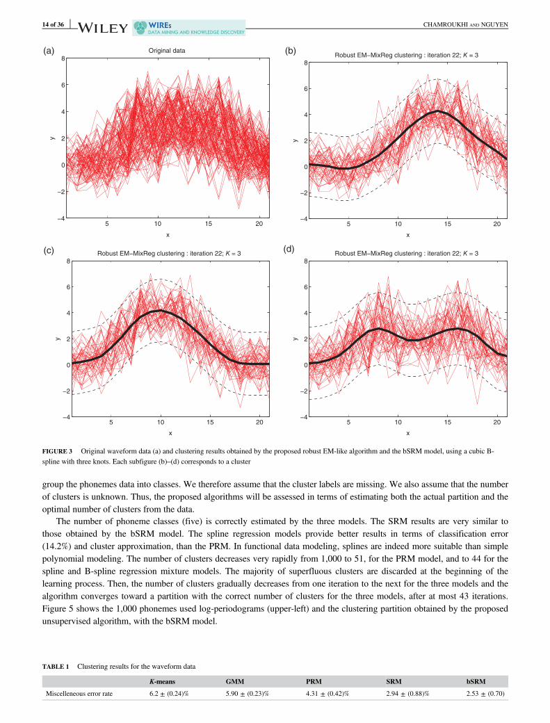
We consider the waveform curves of Breiman et al. (1984) that has also been studied in Hastie and Tibshirani (1996) and else-where. The waveform data is a three-class problem, where each curve is generated as follows: Yi(t) = uhk(t) + (1 − u)hk(t) +Ei(t) for class k where u is a uniform random variable on (0, 1), h1(t) = max(6−| t − 11| , 0); h2(t) = h1(t − 4); h3(t) =h1(t + 4); and Ei(t) is a zero-mean unit-variance Gaussian noise variable. The temporal interval considered for each curve is[1, 21], with a constant period of sampling of 1. Figure 3 shows the corresponding clustering of the waveform data via the B-spline regression mixtures. Each subfigure corresponds to a cluster.

The solid line corresponds to the estimated mean curve and the dashed lines correspond to the approximate normal confi-dence interval, computed as plus and minus twice the estimated standard deviation of the regression point estimates. The num-ber of clusters is correctly estimated by the proposed algorithm. For these data, the spline regression models provide slightlybetter results in terms of clusters approximation than the PRM (here p = 4).

Table 1 presents the clustering results, averaged over 20 different samples of 500 curves. It includes the estimated numberof clusters, the misclassification error rate, and the absolute error between the true cluster proportions and variances, and theestimated values.

We compared the algorithm for the proposed models to two standard clustering algorithms: K-means clustering, and clus-

tering using GMMs. The GMM density of the observations was assumed to have the form f yið Þ¼PK

k¼1αkN yi;μk;σ2kImi

� �.

The number of clusters was fixed to the true value (i.e., K = 3). For GMMs, the number of clusters can be chosen by usingmodel selection criteria such as the BIC.

For all the models, the true number of clusters is correctly retrieved. The misclassification error rate as well as the parame-ter estimation errors are slightly better for the spline regression models, in particular the B-spline regression mixture. On theother hand, it can be seen that the regression mixture models, with the proposed EM-like algorithm, outperform the standardK-means and standard GMM algorithms. Unlike the GMM algorithm, which requires a two-step procedure to estimate boththe number of clusters and the model parameter, the proposed algorithm simultaneously infers the model parameter values andits optimal number of components.

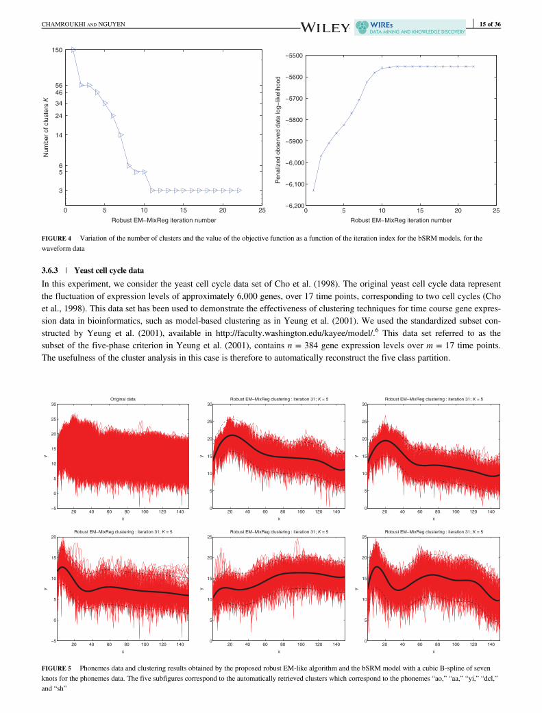
In Figure 4, one can see the variation of the estimated number of clusters as well as the value of the objective functionfrom one iteration to another. These results highlight the capability of the proposed algorithm to provide an accurate partition-ing, with an optimal number of clusters.

In summary, the number of clusters is correctly estimated by the proposed algorithm for three proposed models. Furthermore, theregression mixture models with the proposed EM-like algorithm outperform the standard K-means and GMM clustering methods.

3.6.2 | Phonemes data

The phonemes data set used in Ferraty and Vieu (2003)5 is a subset of the data available from https://web.stanford.edu/~hastie/ElemStatLearn/datasets/ and is described and used in Hastie et al. (1995). The application context related to this dataset is a phoneme classification problem. The phonemes data correspond to log-periodograms y, constructed from recordingsavailable at different equispaced frequencies x, for different phonemes. The data set contains five classes corresponding to thefollowing five phonemes: “sh” as in “she,” “dcl” as in “dark,” “iy” as in “she,” “aa” as in “dark,” and “ao” as in “water”.

For each phoneme, we have 400 log-periodograms at a 16-kHz sampling rate. We only retain the first 150 frequenciesfrom each subject as to conform with the analysis by Ferraty and Vieu (2003). This data set has been considered in a phonemediscrimination problem by Hastie et al. (1995) and Ferraty and Vieu (2003), where the aim was to predict the phoneme classfor a new log-periodogram. Here, we reformulate the problem into a clustering problem, where the aim is to automatically


https://web.stanford.edu/~hastie/ElemStatLearn/datasets/

https://web.stanford.edu/~hastie/ElemStatLearn/datasets/

group the phonemes data into classes. We therefore assume that the cluster labels are missing. We also assume that the numberof clusters is unknown. Thus, the proposed algorithms will be assessed in terms of estimating both the actual partition and theoptimal number of clusters from the data.

The number of phoneme classes (five) is correctly estimated by the three models. The SRM results are very similar tothose obtained by the bSRM model. The spline regression models provide better results in terms of classification error(14.2%) and cluster approximation, than the PRM. In functional data modeling, splines are indeed more suitable than simplepolynomial modeling. The number of clusters decreases very rapidly from 1,000 to 51, for the PRM model, and to 44 for thespline and B-spline regression mixture models. The majority of superfluous clusters are discarded at the beginning of thelearning process. Then, the number of clusters gradually decreases from one iteration to the next for the three models and thealgorithm converges toward a partition with the correct number of clusters for the three models, after at most 43 iterations.Figure 5 shows the 1,000 phonemes used log-periodograms (upper-left) and the clustering partition obtained by the proposedunsupervised algorithm, with the bSRM model.

5 10 15 20−4

−2

0

2

4

6

8y

x

Original data

5 10 15 20−4

−2

0

2

4

6

8

y

x

Robust EM−MixReg clustering : iteration 22; K = 3

5 10 15 20−4

−2

0

2

4

6

8

y

x


5 10 15 20−4

−2

0

2

4

6

8

y

x


(a) (b)

(c) (d)

FIGURE 3 Original waveform data (a) and clustering results obtained by the proposed robust EM-like algorithm and the bSRM model, using a cubic B-spline with three knots. Each subfigure (b)–(d) corresponds to a cluster

TABLE 1 Clustering results for the waveform data

K-means GMM PRM SRM bSRM

Miscelleneous error rate 6.2 ± (0.24)% 5.90 ± (0.23)% 4.31 ± (0.42)% 2.94 ± (0.88)% 2.53 ± (0.70)


3.6.3 | Yeast cell cycle data

In this experiment, we consider the yeast cell cycle data set of Cho et al. (1998). The original yeast cell cycle data representthe fluctuation of expression levels of approximately 6,000 genes, over 17 time points, corresponding to two cell cycles (Choet al., 1998). This data set has been used to demonstrate the effectiveness of clustering techniques for time course gene expres-sion data in bioinformatics, such as model-based clustering as in Yeung et al. (2001). We used the standardized subset con-structed by Yeung et al. (2001), available in http://faculty.washington.edu/kayee/model/.6 This data set referred to as thesubset of the five-phase criterion in Yeung et al. (2001), contains n = 384 gene expression levels over m = 17 time points.The usefulness of the cluster analysis in this case is therefore to automatically reconstruct the five class partition.

0 5 10 15 20 25

3

56

14

24

34

4656

150

Robust EM−MixReg iteration number

Num

ber

of clu

ste

rs K

0 5 10 15 20 25−6,200

−6,100

−6,000

−5900

−5800

−5700

−5600

−5500

Robust EM−MixReg iteration number

Penaliz

ed o

bserv

ed d

ata

log−

likelih

ood

FIGURE 4 Variation of the number of clusters and the value of the objective function as a function of the iteration index for the bSRM models, for thewaveform data

20 40 60 80 100 120 140−5

0

5

10

15

20

25

30

y

x

Original data

20 40 60 80 100 120 1400

5

10

15

20

25

30

y

x


20 40 60 80 100 120 1400

5

10

15

20

25

30

y

x


20 40 60 80 100 120 140−5

0

5

10

15

20

y

x


20 40 60 80 100 120 1400

5

10

15

20

25

y

x


20 40 60 80 100 120 1400

5

10

15

20

25

y

x


FIGURE 5 Phonemes data and clustering results obtained by the proposed robust EM-like algorithm and the bSRM model with a cubic B-spline of sevenknots for the phonemes data. The five subfigures correspond to the automatically retrieved clusters which correspond to the phonemes “ao,” “aa,” “yi,” “dcl,”and “sh”


http://faculty.washington.edu/kayee/model/

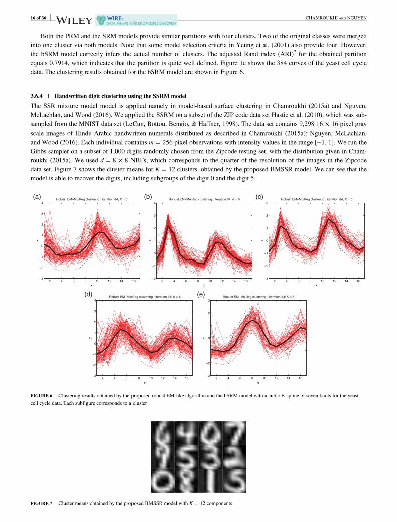
Both the PRM and the SRM models provide similar partitions with four clusters. Two of the original classes were mergedinto one cluster via both models. Note that some model selection criteria in Yeung et al. (2001) also provide four. However,the bSRM model correctly infers the actual number of clusters. The adjusted Rand index (ARI)7 for the obtained partitionequals 0.7914, which indicates that the partition is quite well defined. Figure 1c shows the 384 curves of the yeast cell cycledata. The clustering results obtained for the bSRM model are shown in Figure 6.

3.6.4 | Handwritten digit clustering using the SSRM model

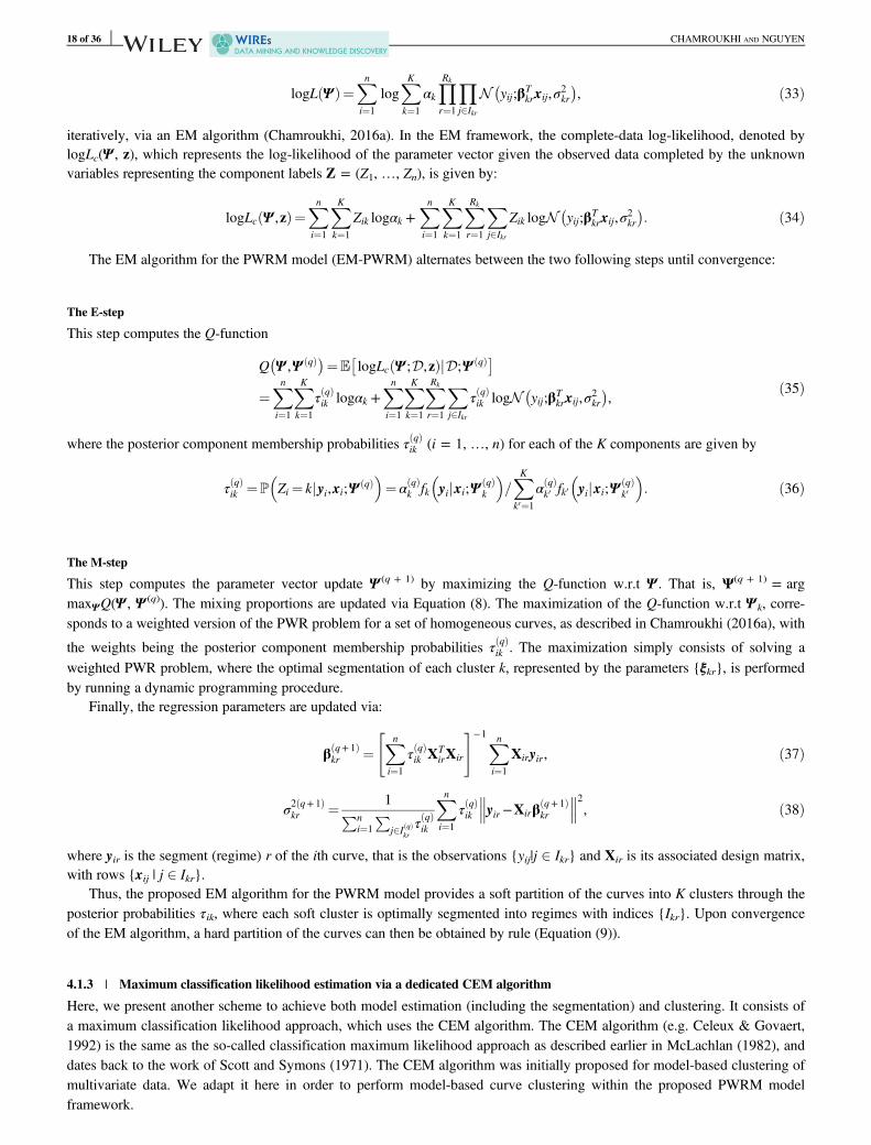
The SSR mixture model model is applied namely in model-based surface clustering in Chamroukhi (2015a) and Nguyen,McLachlan, and Wood (2016). We applied the SSRM on a subset of the ZIP code data set Hastie et al. (2010), which was sub-sampled from the MNIST data set (LeCun, Bottou, Bengio, & Haffner, 1998). The data set contains 9,298 16 × 16 pixel grayscale images of Hindu-Arabic handwritten numerals distributed as described in Chamroukhi (2015a); Nguyen, McLachlan,and Wood (2016). Each individual contains m = 256 pixel observations with intensity values in the range [−1, 1]. We run theGibbs sampler on a subset of 1,000 digits randomly chosen from the Zipcode testing set, with the distribution given in Cham-roukhi (2015a). We used d = 8 × 8 NBFs, which corresponds to the quarter of the resolution of the images in the Zipcodedata set. Figure 7 shows the cluster means for K = 12 clusters, obtained by the proposed BMSSR model. We can see that themodel is able to recover the digits, including subgroups of the digit 0 and the digit 5.

2 4 6 8 10 12 14 16−3

−2

−1

0

1

2

3

4

y

x


2 4 6 8 10 12 14 16−2

−1

0

1

2

3

4

y

x


2 4 6 8 10 12 14 16−3

−2

−1

0

1

2

3

y

x


2 4 6 8 10 12 14 16−3

−2

−1

0

1

2

3

4

y

x


2 4 6 8 10 12 14 16−3

−2

−1

0

1

2

3

y

x


(a) (b) (c)

(d) (e)

FIGURE 6 Clustering results obtained by the proposed robust EM-like algorithm and the bSRM model with a cubic B-spline of seven knots for the yeastcell cycle data. Each subfigure corresponds to a cluster

FIGURE 7 Cluster means obtained by the proposed BMSSR model with K = 12 components


4 | LATENT PROCESS REGRESSION MIXTURES FOR FUNCTIONAL DATA CLUSTERINGAND SEGMENTATION

In the previous section, we presented regression mixtures models for clustering unlabeled functions. We now focus on func-tions with regime changes, possibly smooth, for which the previous methods are unsuitable.

In the models we present, the mixture component density fk(y|x) in Equation (1) is itself assumed to exhibit a complexstructure consisting of subcomponents, each one associated with a regime. In what follows, we investigate three choices forthis component-specific density. That is, first a piecewise regression (PWR) density, then a hidden Markov regression(HMMR) density, and finally a regression model with hidden logistic process (RHLP) density.

4.1 | Mixture of PWRs for functional data clustering and segmentation

The idea described here and proposed in Chamroukhi (2016a) is in the same spirit of the one proposed by Hébrailet al. (2010) for curve clustering and optimal segmentation based on a PWR model that allows for fitting several constant(or polynomial) models to each cluster of functional data with regime changes. However, unlike the distance-based approachof Hébrail et al. (2010), which uses a K-means-like algorithm, the proposed model provides a general probabilistic frameworkto address the problem. Indeed, in the proposed approach, the PWR model is included in a mixture framework, to generalizethe deterministic K-means-like approach. As a result, both soft clustering and hard clustering are possible. We also providetwo algorithms for learning the model parameters.

4.1.1 | The model

The PWRM model assumes that each discrete curve sample (xi, yi) is generated by a PWR model, among K models, with aprior probability αk. That is, each component density in Equation (1) is a PWR model, defined by:

fk yijxi;Ψ kð Þ¼YRk

r¼1

Yj2Ikr

N yij;βTkrxij,σ

2kr

� �ð31Þ

where Ikr = (ξkr, ξk, r + 1] represents the element indices of segment (regime) r (r = 1, …, Rk) for component k, Rk is the corre-sponding number of segments, βkr is the vector of polynomial coefficients, and σ2kr is the associated Gaussian noise variance.Thus, the PWRM density is defined by:


αkYRk

r¼1

Yj2Ikr

N yij;βTkrxij,σ

2kr

� �, ð32Þ

where the parameter vector is given by Ψ ¼ α1,…,αK−1,θT1 ,…,θTK ,ξT1 ,…,ξTK

� �T, and θk ¼ βT

k1,…,βTkRk

,σ2k1,…,σ2kRk

� �Tand

ξk ¼ ξk1,…,ξk,Rk +1

� �T are the vector of all the polynomial coefficients and noise variances, and the vector of transition pointswhich define the segmentation of cluster k, respectively.

The proposed mixture model is therefore suitable for clustering and optimal segmentation of complex-shaped curves. Morespecifically, by integrating the piecewise polynomial regression into the mixture framework, the resulting model is able toapproximate curves from different clusters. Furthermore, the regime changes within each cluster of curves are addressed aswell, due to the optimal segmentation provided by dynamic programming for each PWR component. These two simultaneousoutputs are clearly not provided by the standard regression mixtures. On the other hand, the PWRM is a probabilistic modeland as it will be shown in the sequel that it generalizes the deterministic K-means-like algorithm.

We presented two approaches for learning the model parameters. The former is a dedicated EM algorithm for MLE. A softpartition of the curves into K clusters is then obtained by maximizing the posterior component probabilities. The latter, how-ever, focuses on the classification and optimizes a specific classification likelihood criterion through a dedicated CEM algo-rithm. The optimal curve segmentation is performed via dynamic programming.

In the classification approach, both the curve clustering and the optimal segmentation are performed simultaneously as theCEM algorithm proceeds. We show that the classification approach using the PWRM model with the CEM algorithm is theprobabilistic generalization of the deterministic K-means-like algorithm proposed in Hébrail et al. (2010).

4.1.2 | Maximum likelihood estimation via a dedicated EM algorithm

In MLE approach, the parameter estimation is performed by monotonically maximizing the log-likelihood



logXKk¼1

αkYRk

r¼1

Yj2Ikr

N yij;βTkrxij,σ

2kr

� �, ð33Þ

iteratively, via an EM algorithm (Chamroukhi, 2016a). In the EM framework, the complete-data log-likelihood, denoted bylogLc(Ψ , z), which represents the log-likelihood of the parameter vector given the observed data completed by the unknownvariables representing the component labels Z = (Z1, …, Zn), is given by:

logLc Ψ ,zð Þ¼Xni¼1

XKk¼1

Zik logαk +Xni¼1

XKk¼1

XRk

r¼1

Xj2Ikr

Zik logN yij;βTkrxij,σ

2kr

� �: ð34Þ

The EM algorithm for the PWRM model (EM-PWRM) alternates between the two following steps until convergence:

The E-step

This step computes the Q-function

Q Ψ ,Ψ qð Þ� �¼E logLc Ψ ;D,zð ÞjD;Ψ qð Þ� �

¼Xni¼1

XKk¼1

τ qð Þik logαk +

Xni¼1

XKk¼1

XRk

r¼1

Xj2Ikr

τ qð Þik logN yij;βT

krxij,σ2kr

� �,

ð35Þ

where the posterior component membership probabilities τ qð Þik (i = 1, …, n) for each of the K components are given by

τ qð Þik ¼P Zi ¼ kjyi,xi;Ψ qð Þ

� �¼ α qð Þ

k fk yijxi;Ψqð Þk

� �=XKk0¼1

α qð Þk0 fk0 yijxi;Ψ

qð Þk0

� �: ð36Þ

The M-step

This step computes the parameter vector update Ψ (q + 1) by maximizing the Q-function w.r.t Ψ . That is, Ψ(q + 1) = argmaxΨQ(Ψ , Ψ (q)). The mixing proportions are updated via Equation (8). The maximization of the Q-function w.r.t Ψ k, corre-sponds to a weighted version of the PWR problem for a set of homogeneous curves, as described in Chamroukhi (2016a), with

the weights being the posterior component membership probabilities τ qð Þik . The maximization simply consists of solving a

weighted PWR problem, where the optimal segmentation of each cluster k, represented by the parameters {ξkr}, is performedby running a dynamic programming procedure.

Finally, the regression parameters are updated via:

β q+1ð Þkr ¼

Xni¼1

τ qð Þik XT

irXir

" #−1Xni¼1

Xiryir, ð37Þ

σ2 q+1ð Þkr ¼ 1Pn

i¼1

Pj2I qð Þ

krτ qð Þik

Xni¼1

τ qð Þik yir−Xirβ q+1ð Þ

kr

2, ð38Þ

where yir is the segment (regime) r of the ith curve, that is the observations {yij|j 2 Ikr} and Xir is its associated design matrix,with rows {xij | j 2 Ikr}.

Thus, the proposed EM algorithm for the PWRM model provides a soft partition of the curves into K clusters through theposterior probabilities τik, where each soft cluster is optimally segmented into regimes with indices {Ikr}. Upon convergenceof the EM algorithm, a hard partition of the curves can then be obtained by rule (Equation (9)).

4.1.3 | Maximum classification likelihood estimation via a dedicated CEM algorithm

Here, we present another scheme to achieve both model estimation (including the segmentation) and clustering. It consists ofa maximum classification likelihood approach, which uses the CEM algorithm. The CEM algorithm (e.g. Celeux & Govaert,1992) is the same as the so-called classification maximum likelihood approach as described earlier in McLachlan (1982), anddates back to the work of Scott and Symons (1971). The CEM algorithm was initially proposed for model-based clustering ofmultivariate data. We adapt it here in order to perform model-based curve clustering within the proposed PWRM modelframework.


The resulting CEM algorithm simultaneously estimates the PWRM parameters and the cluster allocations, by maximizingthe complete-data log-likelihood (34) w.r.t both the model parameters Ψ and the partition represented by the vector of clusterlabels z, in an iterative manner, by alternating between the two following steps:

Step 1

Update the cluster labels given the current model parameter Ψ (q), by maximizing the complete-data log-likelihood (34) w.r.tthe cluster labels z: z(q + 1) = arg maxz log Lc(Ψ

(q), z).

Step 2

Given the estimated partition defined by z(q + 1), update the model parameters by maximizing Equation (34) w.r.t to Ψ : Ψ (q + 1) =arg maxΨ log Lc(Ψ , z(q + 1)). Equivalently, the CEM algorithm consists in integrating a classification step (C-step) between theE- and the M-steps of the EM algorithm, presented previously. The C-step computes a hard partition of the n curves intoK clusters by applying rule (Equation (9)).

The difference between this CEM algorithm and the EM algorithm is that the posterior probabilities τik in the case of theEM-PWRM algorithm are replaced by the cluster label indicators Zik in the CEM-PWRM algorithm. That is the curves areassigned in a hard way, rather than in a soft way. By doing so, the CEM monotonically maximizes the complete-data log-likelhood (Equation (34)). Another attractive feature of the proposed PWRM model is that when it is estimated by the CEMalgorithm, as shown in Chamroukhi (2016a), it is a probabilistic generalization of the K-means-like algorithm of Hébrailet al. (2010). Indeed, maximizing the complete-data log-likelihood (Equation (34)) optimized by the proposed CEM algorithmfor the PWRM model, is equivalent to minimizing the following distortion criterion w.r.t the cluster labels z, the segmentsindices Ikr and the segments constant means μkr, which is exactly the criterion optimized by the K-means-like algorithm:

J z, μkr ,Ikrf gð Þ¼PK

k¼1

PRkr¼1

PijZi¼k

Pj2Ikr yij−μkr� �2, if the constraints αk ¼ 1

K.

8K (identical mixing proportions), and σ2kr ¼ σ2 for all r = 1, …, Rk and k = 1, …, K (isotropic and homoskedastic model)are imposed, in addition to the use of a piecewise constant approximation of each segment rather than a polynomial approxi-mation. The proposed CEM algorithm for piecewise PRM is therefore the probabilistic version for hard curve clustering andoptimal segmentation of the K-means-like algorithm.

4.1.4 | Experiments

The performance of the PWRM with both the EM and CEM algorithms has been studied in Chamroukhi (2016a) by compar-ing it to the PRM models (Gaffney, 2004), the standard polynomial spline regression mixture model (PSRM) (Gaffney, 2004;Gui & Li, 2003; Liu & Yang, 2009) and the PWR model implemented via the K-means-like algorithm (Hébrail et al., 2010).Comparisons with standard model-based clustering methods for multivariate data, including the GMM, were also considered.

Simulation results

The considered evaluation criteria are the classification error rate between the true partition and the estimated partition, andthe intracluster inertia. In these simulation studies, in the situations where all the considered algorithms have close clusteringaccuracy, the standard model-based clustering approach using the GMM have poor performance in terms of curves approxi-mation. This is due to the fact that using the GMM is not appropriate for this context as it does not take into account the func-tional structure of the curves and computes an overall mean curve. On the other hand, the proposed probabilistic model, whentrained with the EM algorithm (EM-PWRM) or with the CEM algorithm (CEM-PWRM) as well as the K-means-like algo-rithm of Hébrail et al. (2010), as expected, provide nearly identical results in terms of clustering and segmentation. This isattributed to the fact that the K-means PWRM approach is a particular case of the proposed probabilistic approach.

The best curve approximations, however, are those provided by the PWRM models. The GMM curves are simply means,and the PRM and the PSRM models, as they are based on continuous curve models, do not account for the segmentation,unlike the PWRM models, which are better suited for simultaneous curve clustering and segmentation.

When we increased the noise level, the misclassification error rate increases faster for the other models, compared to thoseof the proposed PWRM model. The EM and the CEM algorithm for the proposed approach provide very similar results, witha slight advantage for the CEM version, which can be attributed to the fact that CEM is by construction tailored to classifica-tion. When the proposed PWRM approach is used, the misclassification error can be improved by 4% compared to the K-means-like approach, about 7% compared to both the PRM and the PSRM, and more that 15% compared to the standard multi-variate GMM. In addition, when the data have nonuniform mixing proportions, the K-means-like approach, can fail namely interms of segmentation. This is attributed to the fact that the K-means-like approach for PWRM is constrained, as it assumesthe same proportion for each cluster, and does not sufficiently take into account the heteroskedasticity within each cluster.


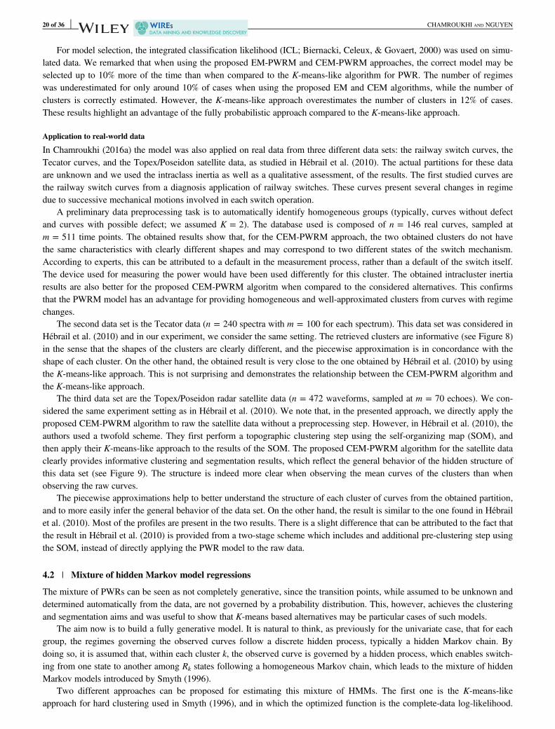
For model selection, the integrated classification likelihood (ICL; Biernacki, Celeux, & Govaert, 2000) was used on simu-lated data. We remarked that when using the proposed EM-PWRM and CEM-PWRM approaches, the correct model may beselected up to 10% more of the time than when compared to the K-means-like algorithm for PWR. The number of regimeswas underestimated for only around 10% of cases when using the proposed EM and CEM algorithms, while the number ofclusters is correctly estimated. However, the K-means-like approach overestimates the number of clusters in 12% of cases.These results highlight an advantage of the fully probabilistic approach compared to the K-means-like approach.

Application to real-world data

In Chamroukhi (2016a) the model was also applied on real data from three different data sets: the railway switch curves, theTecator curves, and the Topex/Poseidon satellite data, as studied in Hébrail et al. (2010). The actual partitions for these dataare unknown and we used the intraclass inertia as well as a qualitative assessment, of the results. The first studied curves arethe railway switch curves from a diagnosis application of railway switches. These curves present several changes in regimedue to successive mechanical motions involved in each switch operation.

A preliminary data preprocessing task is to automatically identify homogeneous groups (typically, curves without defectand curves with possible defect; we assumed K = 2). The database used is composed of n = 146 real curves, sampled atm = 511 time points. The obtained results show that, for the CEM-PWRM approach, the two obtained clusters do not havethe same characteristics with clearly different shapes and may correspond to two different states of the switch mechanism.According to experts, this can be attributed to a default in the measurement process, rather than a default of the switch itself.The device used for measuring the power would have been used differently for this cluster. The obtained intracluster inertiaresults are also better for the proposed CEM-PWRM algoritm when compared to the considered alternatives. This confirmsthat the PWRM model has an advantage for providing homogeneous and well-approximated clusters from curves with regimechanges.

The second data set is the Tecator data (n = 240 spectra with m = 100 for each spectrum). This data set was considered inHébrail et al. (2010) and in our experiment, we consider the same setting. The retrieved clusters are informative (see Figure 8)in the sense that the shapes of the clusters are clearly different, and the piecewise approximation is in concordance with theshape of each cluster. On the other hand, the obtained result is very close to the one obtained by Hébrail et al. (2010) by usingthe K-means-like approach. This is not surprising and demonstrates the relationship between the CEM-PWRM algorithm andthe K-means-like approach.

The third data set are the Topex/Poseidon radar satellite data (n = 472 waveforms, sampled at m = 70 echoes). We con-sidered the same experiment setting as in Hébrail et al. (2010). We note that, in the presented approach, we directly apply theproposed CEM-PWRM algorithm to raw the satellite data without a preprocessing step. However, in Hébrail et al. (2010), theauthors used a twofold scheme. They first perform a topographic clustering step using the self-organizing map (SOM), andthen apply their K-means-like approach to the results of the SOM. The proposed CEM-PWRM algorithm for the satellite dataclearly provides informative clustering and segmentation results, which reflect the general behavior of the hidden structure ofthis data set (see Figure 9). The structure is indeed more clear when observing the mean curves of the clusters than whenobserving the raw curves.

The piecewise approximations help to better understand the structure of each cluster of curves from the obtained partition,and to more easily infer the general behavior of the data set. On the other hand, the result is similar to the one found in Hébrailet al. (2010). Most of the profiles are present in the two results. There is a slight difference that can be attributed to the fact thatthe result in Hébrail et al. (2010) is provided from a two-stage scheme which includes and additional pre-clustering step usingthe SOM, instead of directly applying the PWR model to the raw data.

4.2 | Mixture of hidden Markov model regressions

The mixture of PWRs can be seen as not completely generative, since the transition points, while assumed to be unknown anddetermined automatically from the data, are not governed by a probability distribution. This, however, achieves the clusteringand segmentation aims and was useful to show that K-means based alternatives may be particular cases of such models.

The aim now is to build a fully generative model. It is natural to think, as previously for the univariate case, that for eachgroup, the regimes governing the observed curves follow a discrete hidden process, typically a hidden Markov chain. Bydoing so, it is assumed that, within each cluster k, the observed curve is governed by a hidden process, which enables switch-ing from one state to another among Rk states following a homogeneous Markov chain, which leads to the mixture of hiddenMarkov models introduced by Smyth (1996).

Two different approaches can be proposed for estimating this mixture of HMMs. The first one is the K-means-likeapproach for hard clustering used in Smyth (1996), and in which the optimized function is the complete-data log-likelihood.


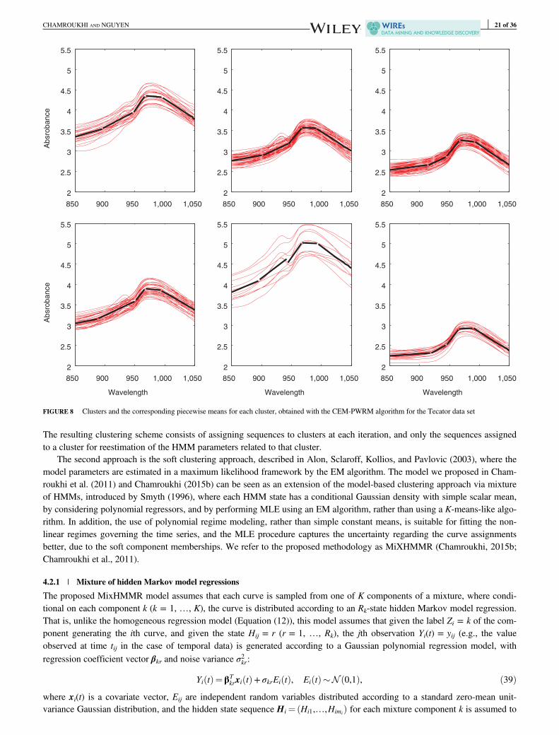
The resulting clustering scheme consists of assigning sequences to clusters at each iteration, and only the sequences assignedto a cluster for reestimation of the HMM parameters related to that cluster.

The second approach is the soft clustering approach, described in Alon, Sclaroff, Kollios, and Pavlovic (2003), where themodel parameters are estimated in a maximum likelihood framework by the EM algorithm. The model we proposed in Cham-roukhi et al. (2011) and Chamroukhi (2015b) can be seen as an extension of the model-based clustering approach via mixtureof HMMs, introduced by Smyth (1996), where each HMM state has a conditional Gaussian density with simple scalar mean,by considering polynomial regressors, and by performing MLE using an EM algorithm, rather than using a K-means-like algo-rithm. In addition, the use of polynomial regime modeling, rather than simple constant means, is suitable for fitting the non-linear regimes governing the time series, and the MLE procedure captures the uncertainty regarding the curve assignmentsbetter, due to the soft component memberships. We refer to the proposed methodology as MiXHMMR (Chamroukhi, 2015b;Chamroukhi et al., 2011).

4.2.1 | Mixture of hidden Markov model regressions

The proposed MixHMMR model assumes that each curve is sampled from one of K components of a mixture, where condi-tional on each component k (k = 1, …, K), the curve is distributed according to an Rk-state hidden Markov model regression.That is, unlike the homogeneous regression model (Equation (12)), this model assumes that given the label Zi = k of the com-ponent generating the ith curve, and given the state Hij = r (r = 1, …, Rk), the jth observation Yi(t) = yij (e.g., the valueobserved at time tij in the case of temporal data) is generated according to a Gaussian polynomial regression model, withregression coefficient vector βkr and noise variance σ2kr:

Yi tð Þ¼βTkrxi tð Þ+ σkrEi tð Þ, Ei tð Þ�N 0,1ð Þ, ð39Þ

where xi(t) is a covariate vector, Eij are independent random variables distributed according to a standard zero-mean unit-variance Gaussian distribution, and the hidden state sequence Hi ¼ Hi1,…,Himið Þ for each mixture component k is assumed to

850 900 950 1,000 1,050

2

2.5

3

3.5

4

4.5

5

5.5A

bsro

bance

850 900 950 1,000 1,050

2

2.5

3

3.5

4

4.5

5

5.5

850 900 950 1,000 1,050

2

2.5

3

3.5

4

4.5

5

5.5

850 900 950 1,000 1,050

2

2.5

3

3.5

4

4.5

5

5.5

Absro

bance

Wavelength

850 900 950 1,000 1,050

2

2.5

3

3.5

4

4.5

5

5.5

Wavelength

850 900 950 1,000 1,050

2

2.5

3

3.5

4

4.5

5

5.5

Wavelength

FIGURE 8 Clusters and the corresponding piecewise means for each cluster, obtained with the CEM-PWRM algorithm for the Tecator data set


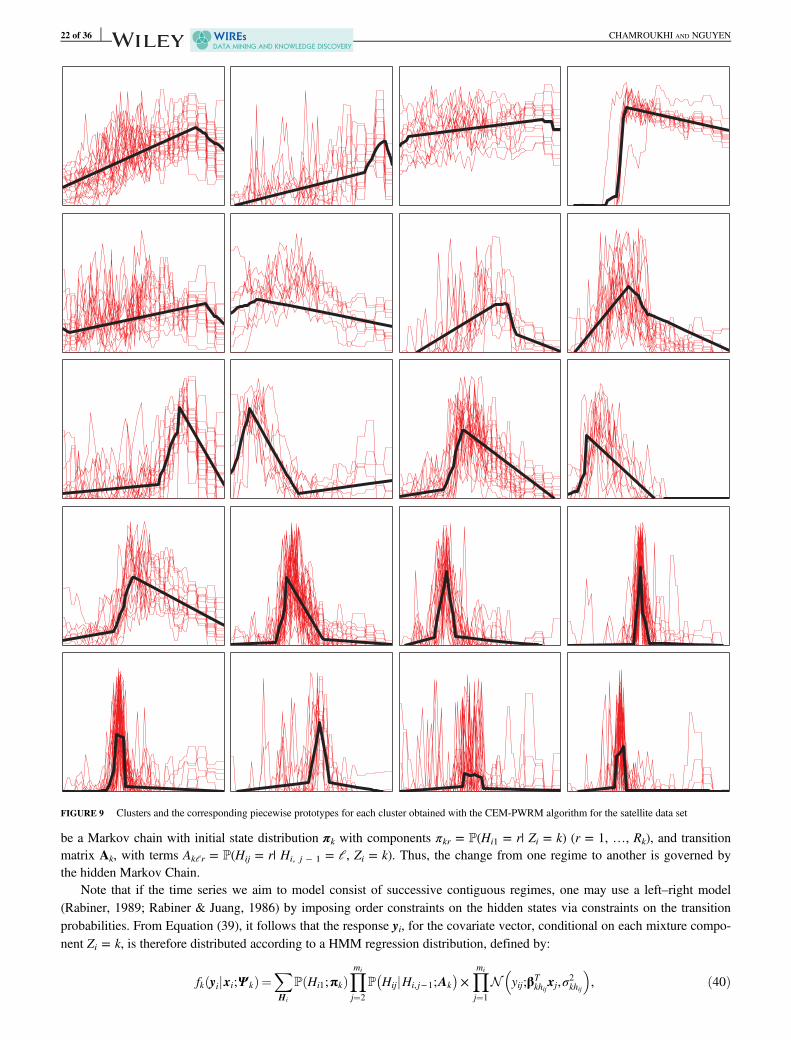
be a Markov chain with initial state distribution πk with components πkr = P(Hi1 = r| Zi = k) (r = 1, …, Rk), and transitionmatrix Ak, with terms Akℓr = P(Hij = r| Hi, j − 1 = ℓ, Zi = k). Thus, the change from one regime to another is governed bythe hidden Markov Chain.

Note that if the time series we aim to model consist of successive contiguous regimes, one may use a left–right model(Rabiner, 1989; Rabiner & Juang, 1986) by imposing order constraints on the hidden states via constraints on the transitionprobabilities. From Equation (39), it follows that the response yi, for the covariate vector, conditional on each mixture compo-nent Zi = k, is therefore distributed according to a HMM regression distribution, defined by:

fk yijxi;Ψ kð Þ¼XHi

P Hi1;πkð ÞYmi

j¼2

P HijjHi, j−1;Ak� �

×Ymi

j¼1

N yij;βTkhijxj,σ

2khij

� �, ð40Þ

FIGURE 9 Clusters and the corresponding piecewise prototypes for each cluster obtained with the CEM-PWRM algorithm for the satellite data set


with parameter vector Ψ k ¼ πTk ,vec Akð ÞT ,βT

k1,…,βTkR,σ

2k1,…,σ2kR

� �Twhere vec(�) is the vectorization of a matrix. Finally, the

distribution of a curve (xi, yi) is defined by the following MixHMMR density:


αkfk yijxi;Ψ kð Þ, ð41Þ

described by the parameter vector Ψ ¼ α1,…,αK−1,Ψ T1 ,…,Ψ T

K

� �T.


The MixHMMR parameter vector Ψ is estimated by monotonically maximizing the log-likelihood


logXKk¼1

αkXHi

P Hi1;πkð ÞYmi

j¼2

P HijjHi, j−1;Ak� �

×Ymi

j¼1

N yij;βTkhijxj,σ

2khij

� �, ð42Þ

using a dedicated EM algorithm as devoloped in Chamroukhi et al. (2011) and Chamroukhi (2015b). By introducing the twoindicator binary variables for indicating the cluster memberships and the regime memberships for a given cluster, that is, Zik =1 if Zi = k (i.e., yi belongs to cluster k) and Zik = 0 otherwise, and Hijr = 1 if Hij = r (i.e., the ith time series yi belongs tocluster k and its jth observation yij at time tj belongs to regime r) and Hijr = 0 otherwise, the complete-data likelihood of Ψcan be written as:

logLc Ψð Þ¼XKk¼1

Xi

Zik logαk +Xi,r

ZikHi1r logπkr +X

i, j¼2,r,ℓZikHijrHi j−1ð Þℓ logAkℓr

"

+Xi, j,r

ZikHijr logN yij;βTkrxj,σ

2kr

� �#�

ð43Þ

The EM algorithm for the MixHMMR model starts from an initial parameter Ψ (0) (see Chamroukhi et al. (2011) for an ini-tialization strategy) and alternates between the two following steps until convergence:

4.2.3 | The E-Step

This step computes the conditional expected complete-data log-likelihood: Q Ψ ,Ψ qð Þ� �¼E logLc Ψð ÞjD;Ψ qð Þ� �

which isgiven by:

Q Ψ ,Ψ qð Þ� �

¼Xk, i


Xk

Xr, i

τ qð Þik γ qð Þ

i1r logπkr +Xj¼2,ℓ

ξ qð Þijℓr logAkℓr

" #+Xmi

r, i, jτ qð Þik γ qð Þ

ijr logN yij;βTkrxj,σ

2kr

� �" #ð44Þ

and therefore only requires the computation of the posterior probabilities τ qð Þik , γ qð Þ

ijr , and ξ qð Þijℓr , where

• τ qð Þik ¼P Zi ¼ kjyi,xi;Ψ qð Þ� �

is the posterior probability that the ith curve belongs to the kth mixture component;

• γ qð Þijr ¼P Hij ¼ rjyi,xi;Ψ

qð Þk

� �is the posterior probability of the rth polynomial regime in the mixture component k; and

• ξ qð Þijℓr ¼P Hij ¼ r,Hi j−1ð Þ ¼ℓjyi,xi;Ψ

qð Þk

� �is the joint posterior probability of having the regime r at time tj and the regime ℓ

at time tj − 1, in component k.

The E-step probabilities γ qð Þijr and ξ qð Þ

ijℓr for each time series yi (i = 1, …, n) are computed recursively by using the forward-

backward algorithm (see Chamroukhi et al., 2011; Rabiner, 1989; Rabiner & Juang, 1986). The posterior probabilities τ qð Þik are

given by:

τ qð Þik ¼ α qð Þ


� �=XKk0¼1


qð Þk0

� �, ð45Þ

where the conditional probability distribution fk yijxi;Ψqð Þk

� �is that of a HMM regression likelihood (given by Equation (40)),

and is obtained after the forward procedure when fitting a standard HMM.


4.2.4 | The M-Step

This step computes the parameter vector update Ψ (q + 1), by maximizing the expected complete-data log-likelihood(i.e., Ψ (q + 1) = arg maxΨQ(Ψ , Ψ (q))). The maximization w.r.t the mixing proportions is same as for a standard mixture modelgiven by Equation (8). The maximization w.r.t the Markov chain parameters πk and Ak correspond to a weighted version ofupdating the parameters of the Markov chain in a standard HMM, where the weights in this case are the posterior component

membership probabilities τ qð Þik . The updates are given by:

π q+1ð Þkr ¼

Pni¼1 τ

qð Þik γ qð Þ

i1rPni¼1 τ

qð Þik

,

A q+1ð Þkℓr ¼

Pni¼1

Pmij¼2 τ

qð Þik ξ qð Þ

ijℓrPni¼1

Pmij¼2 τ

qð Þik γ qð Þ

ijr

�

Finally, the maximization w.r.t the regression parameters βkr consists of analytically solving weighted least-squares prob-lems and the update w.r.t the noise variances σ2kr is a weighted variant of the problem of estimating the variance of a univariateGaussian density.

The weights consist of both the posterior cluster probabilities τik and the posterior regime probabilities γ qð Þijr for each cluster

k. The parameter updates are given by:

β q+1ð Þkr ¼

Xni¼1

τ qð Þik XT

i Wqð ÞikrXi

" #−1Xni¼1

τ qð Þik XT

i Wqð Þikr yi, ð46Þ

σ2 q+1ð Þkr ¼

Pni¼1 τ

qð Þik

ffiffiffiffiffiffiffiffiffiffiW qð Þ

ikr

qyi−Xiβ q+1ð Þ

kr

� � 2

Pni¼1 τ

qð Þik trace W qð Þ

ikr

� � , ð47Þ

where W qð Þikr is an mi × mi diagonal matrix whose diagonal elements are the weights γ qð Þ

ijr ;j¼ 1,…,mi

n o. It can be seen that the

parameters for each regime are updated from the whole curve weighted by the posterior regime memberships {γijr}, while inthe previously presented PWR models, they are only updated from the observations assigned to that regime, that is, in a hardmanner. This better takes into account possible uncertainty regarding whether the regime change in abrupt or not.

4.2.5 | Experiments

The performance of the MixHMMR model was studied in Chamroukhi et al. (2011) by comparing it to the regression mixturemodel, the standard mixture of HMMs, as well as the GMM and K-means algorithms.

4.2.6 | Simulation results

The evaluation criteria used in the simulations are the misclassification error rate between the true simulated partition and theestimated partition, and the intracluster inertia. From the obtained results, it was observed that the proposed approach providesmore accurate classification results and smaller intraclass inertias compared to the considered alternatives. For example, theMixHMMR provides a clustering error 3% less than the standard mixture of HMMs, which is the most competitive model,and more than 10% less compared to the GMM and K-means methods. Applying the MixHMMR for clustering time serieswith regime changes also provided accurate results in terms of clustering and approximation of each cluster of time series.This can be attributed to the fact that the proposed MixHMMR model, with its flexible generative formulation, addresses boththe problems of time series heterogeneity and the dynamical aspect within each homogeneous set of time series, via the under-lying Markov chain.

4.2.7 | Clustering real time series of switch operations

The model was also applied in Chamroukhi et al. (2011) to a real problem of clustering time series for a railway diagnosisapplication. The data set contains n = 115 curves, each resulting from R = 6 electromechanical processes. The model withcubic polynomials (which was enough to approximate each regime) was applied with K = 2 clusters in order to separatecurves that would correspond to a defective operating state and curves corresponding to a normal operating state.

Since the true class labels are unknown, we only considered the intraclass inertias as well as a graphical inspection byobserving the obtained partitions and each cluster approximation. The algorithm provided a partition of curves, where the clus-ter shapes are clearly different (see Figure 10) and may correspond to two different states of the switch mechanism. According


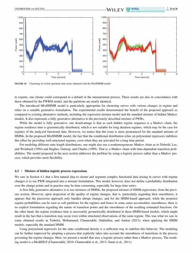
to experts, one cluster could correspond to a default in the measurement process. These results are also in concordance withthose obtained by the PWRM model, and the partitions are nearly identical.

The introduced MixHMMR model is particularly appropriate for clustering curves with various changes in regime andrelies on a suitable generative formulation. The experimental results demonstrated the benefit of the proposed approach ascompared to existing alternative methods, including the regression mixture model and the standard mixture of hidden Markovmodels. It also represents a fully generative alternative to the previously described mixture of PWRs.

While the model is fully generative, one disadvantage is that as each hidden regime sequence is a Markov chain, theregime residence time is geometrically distributed, which is not suitable for long duration regimes, which may be the case forregimes of the analyzed functional data. However, we notice that this issue is more pronounced for the standard mixture ofHMMs. In the proposed MixHMMR model, the fact that the conditional distribution relies on polynomial regressors stabilizesthis effect by providing well-structured regimes, even when they are activated for a long time period.

For modeling different state length distributions, one might also use a nonhomogeneous Markov chain as in Diebold, Lee,and Weinbach (1994) and Hughes, Guttorp, and Charles (1999). That is, a Markov chain with time-dependent transition prob-abilities. The model proposed in the next section addresses the problem by using a logistic process rather than a Markov pro-cess, which provides more flexibility.

4.3 | Mixture of hidden logistic process regressions

We saw in Section 4.1 that a first natural idea to cluster and segment complex functional data arising in curves with regimechanges is to use PWR integrated into a mixture formulation. This model, however, does not define a probability distributionover the change points and in practice may be time consuming, especially for large time series.

A first fully generative alternative is to use mixtures of HMMs, the proposed mixture of HMM regressions, from the previ-ous section. However, upon inspection of the quality of regime changes, that is, particularly regarding their smoothness, itappears that the piecewise approach only handles abrupt changes, and for the HMM-based approach, while the posteriorregime probabilities can be seen as soft partitions for the regimes and hence in some sense accomodates smoothness, there isno explicit formulation regarding the nature of transition points and the smoothness of the resulting estimated functions. Onthe other hand, the regime residence time is necessarily geometrically distributed in these HMM-based models, which mightresult in the fact that a transition may occur even within structured observations of the same regime. This was what we saw insome obtained results in Trabelsi, Mohammed, Chamroukhi, Oukhellou, and Amirat (2013), when applying the HMMmodels, especially the standard HMM.

Using polynomial regressors for the state conditional density is a sufficient way to stabilize this behavior. The modelingcan be further improved by adopting a process that explicitly takes into account the smoothness of transitions in the processgoverning the regime changes. Here, we present a model that uses a logistic process rather than a Markov process. The result-ing model is a MixRHLP (Chamroukhi, 2010; Chamroukhi et al., 2013; Samé et al., 2011).

0 1 2 3 4 5 60

100

200

300

400

500

600

700

800

900

1,000

Time (second)

Po

we

r (w

att)

0 1 2 3 4 5 60

100

200

300

400

500

600

700

800

900

1,000

Time (second)

Po

we

r (w

att)

FIGURE 10 Clustering of switch operation time series obtained with the MixHMMR model


4.3.1 | The model

In the proposed MixRHLP model (Chamroukhi, 2010; Chamroukhi et al., 2013; Samé et al., 2011), each of the functionalmixture components (Equation (1)) is an RHLP (Chamroukhi et al., 2009b, 2010). As presented in Chamroukhi et al. (2009b)and Chamroukhi (2015b), the conditional distribution of a curve is defined by an RHLP:

fk yijxi;Ψ kð Þ¼Ymi

j¼1

XRk

r¼1

πkr xj;wk� �

N yij;βTkrxj,σ

2kr

� �ð48Þ

whose parameter vector is Ψ k ¼ wTk ,β

Tk1,…,βT

kRk,σ2k1,…,σ2kRk

� �Tand where the distribution of the discrete variable Hij govern-

ing the hidden regimes is assumed to be logistic:

πkr xj;wk� �

¼P Hij ¼ rjZi ¼ k,xj;wk� �

¼exp wkr0 +wkr1xj� �

PRk

r0¼1exp wkr00 +wkr01xj� � , ð49Þ

whose parameter vector is wk ¼ wTk1,…,wT

kRk−1

� �T, where wkr = (wkr0, wkr1)

T is the two-dimensional coefficient vector for the

rth logistic component with wkRk being the null vector. This choice is due to the flexibility of the logistic function in bothdetermining the regime transition points and accurately modeling abrupt and/or smooth regime changes. Indeed, as shown inChamroukhi et al. (2009b, 2010), the logistic function (Equation (49)) parameters wkr0 and wkr1 control the regime transitionpoints and the quality of regime (smooth or abrupt).

We remark that a linear logistic function was used for contiguous regime segmentation. The RHLP model can be seen as amixture of experts (Nguyen & Chamroukhi, 2018), where the experts are polynomial regressors and the gating network is alogistic transformation of a linear function of the input x (e.g., the time t in time series). As such, with sufficiently large num-bers of regimes, a RHLP model can model any continuous family of curves (Nguyen, Lloyd-Jones, & McLachlan, 2016). Tohighlight the flexibility of the RHLP model, Figure 11 shows the RHLP model (Equation (48)) fitted to each of the three rail-way switch operation curves, shown in Figure 2, where each operation signal is composed of five successive movements, eachof which is associated with a regime in the RHLP model. The provided results show both flexible segmentation via the logisticprobabilities (middle) and the approximation (top and bottom).

Given the defined model for each of the K components, the resulting density of a curve has the following MixRHLP form:


αkYmi

j¼1

XRk

r¼1

πkr xj;wk� �

N yij;βTkrxj,σ

2kr

� �, ð50Þ

with parameter vector Ψ ¼ α1,…,αK−1,Ψ T1 ,…,Ψ T

K

� �T. Notice that the key difference between the MixRHLP and the standard

regression mixture model is that the proposed model uses a generative hidden process regression model (RHLP) for each com-ponent, rather than polynomial or spline components. The RHLP is itself based on a dynamic mixture formulation. Thus, theproposed approach is more suitable for accomodating regime changes within curves during time.


The unknown parameter vector Ψ is estimated from an i.i.d sample of unlabeled curves D¼ x1,y1ð Þ,…, xn,ynð Þð Þ by monoton-ically maximizing the following log-likelihood


logXKk¼1

αkYmi

j¼1

XRk

r¼1

πkr xj;wk� �

N yij;βTkrxj,σ

2kr

� �,

via a dedicated EM algorithm. The EM scheme requires the definition of the complete-data log-likelihood. The complete-datalog-likelihood for the proposed MixRHLP model, given the observed data which we denote by D, the hidden componentlabels Z, and the hidden process {Hk} for each of the K components, is given by:

logLc Ψð Þ¼Xni¼1

XKk¼1

Zik logαk +Xni¼1

Xmi

j¼1

XKk¼1

XRk

r¼1

ZikHijr log πkr xj;wk� �

N yij;βTkrxj,σ

2kr

� �� : ð51Þ

The EM algorithm for the MixRHLP model (EM-MixRHLP) starts with an initial parameter Ψ (0) (see Chamroukhi, 2010and Samé et al., 2011, for an initialization strategy) and alternates between the two following steps until convergence:


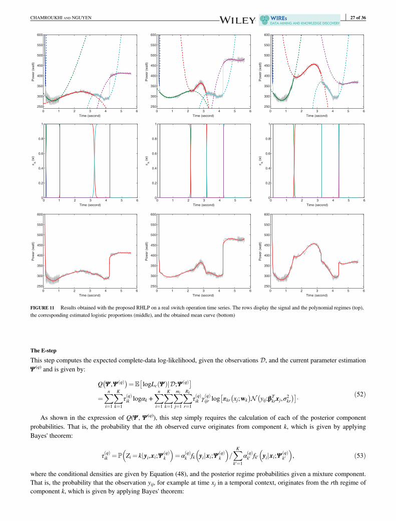
The E-step

This step computes the expected complete-data log-likelihood, given the observations D, and the current parameter estimationΨ (q) and is given by:

Q Ψ ,Ψ qð Þ� �¼E logLc Ψð ÞjD;Ψ qð Þ� �

¼Xni¼1

XKk¼1


Xni¼1

XKk¼1

Xmi

j¼1

XRk

r¼1

τ qð Þik γ qð Þ

ijr log πkr xj;wk� �

N yij;βTkrxj,σ

2kr

� �� ð52Þ

As shown in the expression of Q(Ψ , Ψ (q)), this step simply requires the calculation of each of the posterior componentprobabilities. That is, the probability that the ith observed curve originates from component k, which is given by applyingBayes' theorem:

τ qð Þik ¼P Zi ¼ kjyi,xi;Ψ

qð Þk

� �¼ α qð Þ


� �=XKk0¼1


qð Þk0

� �, ð53Þ

where the conditional densities are given by Equation (48), and the posterior regime probabilities given a mixture component.That is, the probability that the observation yij, for example at time xj in a temporal context, originates from the rth regime ofcomponent k, which is given by applying Bayes' theorem:

0 1 2 3 4 5 6

250

300

350

400

450

500

550

600

Time (second)

Po

we

r (w

att

)

0 1 2 3 4 5 6

250

300

350

400

450

500

550

600

Time (second)

Po

we

r (w

att

)

0 1 2 3 4 5 6

250

300

350

400

450

500

550

600

Time (second)

Po

we

r (w

att

)

0 1 2 3 4 5 60

0.2

0.4

0.6

0.8

1

πik (

w)

Time (second)

0 1 2 3 4 5 60

0.2

0.4

0.6

0.8

1

πik (

w)

Time (second)

0 1 2 3 4 5 60

0.2

0.4

0.6

0.8

1

πik (

w)

Time (second)

0 1 2 3 4 5 6

250

300

350

400

450

500

550

600

Time (second)

Po

we

r (w

att

)

0 1 2 3 4 5 6

250

300

350

400

450

500

550

600

Time (second)

Po

we

r (w

att

)

0 1 2 3 4 5 6

250

300

350

400

450

500

550

600

Time (second)

Po

we

r (w

att

)

FIGURE 11 Results obtained with the proposed RHLP on a real switch operation time series. The rows display the signal and the polynomial regimes (top),the corresponding estimated logistic proportions (middle), and the obtained mean curve (bottom)


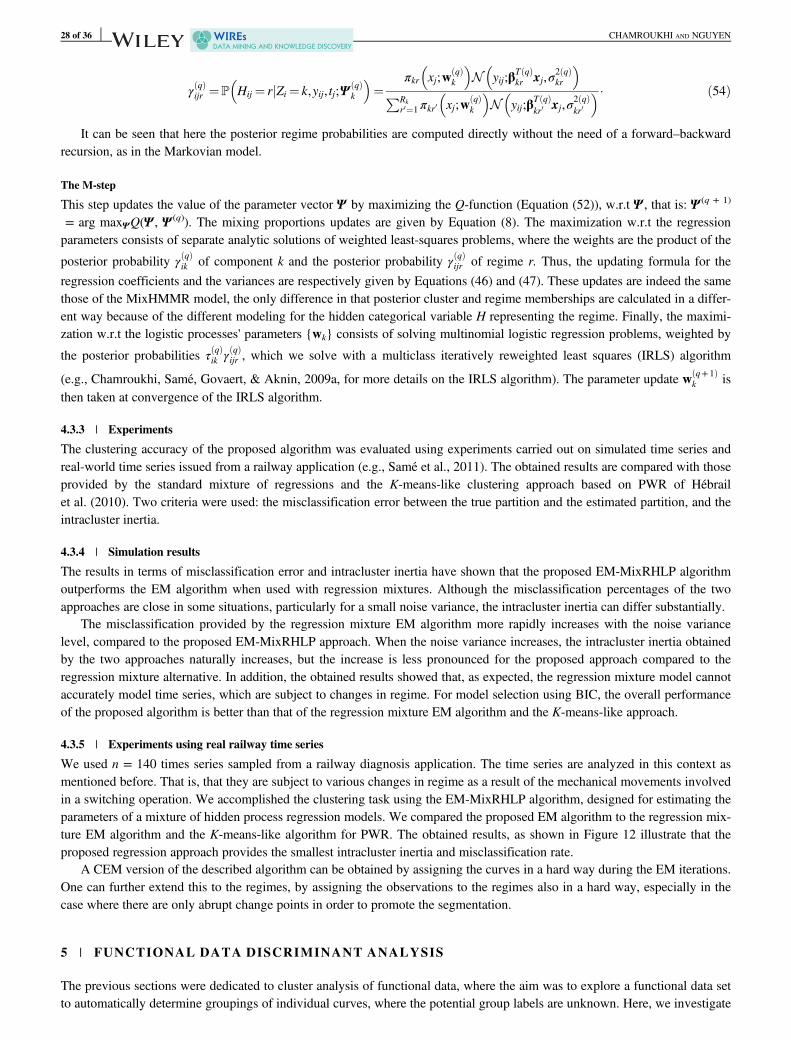
γ qð Þijr ¼P Hij ¼ rjZi ¼ k,yij, tj;Ψ

qð Þk

� �¼

πkr xj;wqð Þk

� �N yij;βT qð Þ

kr xj,σ2 qð Þkr

� �PRk

r0¼1πkr0 xj;wqð Þk

� �N yij;βT qð Þ

kr0 xj,σ2 qð Þkr0

� � � ð54Þ

It can be seen that here the posterior regime probabilities are computed directly without the need of a forward–backwardrecursion, as in the Markovian model.

The M-step

This step updates the value of the parameter vector Ψ by maximizing the Q-function (Equation (52)), w.r.t Ψ , that is: Ψ (q + 1)

= arg maxΨQ(Ψ , Ψ (q)). The mixing proportions updates are given by Equation (8). The maximization w.r.t the regressionparameters consists of separate analytic solutions of weighted least-squares problems, where the weights are the product of the

posterior probability γ qð Þik of component k and the posterior probability γ qð Þ

ijr of regime r. Thus, the updating formula for the

regression coefficients and the variances are respectively given by Equations (46) and (47). These updates are indeed the samethose of the MixHMMR model, the only difference in that posterior cluster and regime memberships are calculated in a differ-ent way because of the different modeling for the hidden categorical variable H representing the regime. Finally, the maximi-zation w.r.t the logistic processes' parameters {wk} consists of solving multinomial logistic regression problems, weighted by

the posterior probabilities τ qð Þik γ qð Þ

ijr , which we solve with a multiclass iteratively reweighted least squares (IRLS) algorithm

(e.g., Chamroukhi, Samé, Govaert, & Aknin, 2009a, for more details on the IRLS algorithm). The parameter update w q+1ð Þk is

then taken at convergence of the IRLS algorithm.

4.3.3 | Experiments

The clustering accuracy of the proposed algorithm was evaluated using experiments carried out on simulated time series andreal-world time series issued from a railway application (e.g., Samé et al., 2011). The obtained results are compared with thoseprovided by the standard mixture of regressions and the K-means-like clustering approach based on PWR of Hébrailet al. (2010). Two criteria were used: the misclassification error between the true partition and the estimated partition, and theintracluster inertia.


The results in terms of misclassification error and intracluster inertia have shown that the proposed EM-MixRHLP algorithmoutperforms the EM algorithm when used with regression mixtures. Although the misclassification percentages of the twoapproaches are close in some situations, particularly for a small noise variance, the intracluster inertia can differ substantially.

The misclassification provided by the regression mixture EM algorithm more rapidly increases with the noise variancelevel, compared to the proposed EM-MixRHLP approach. When the noise variance increases, the intracluster inertia obtainedby the two approaches naturally increases, but the increase is less pronounced for the proposed approach compared to theregression mixture alternative. In addition, the obtained results showed that, as expected, the regression mixture model cannotaccurately model time series, which are subject to changes in regime. For model selection using BIC, the overall performanceof the proposed algorithm is better than that of the regression mixture EM algorithm and the K-means-like approach.

4.3.5 | Experiments using real railway time series

We used n = 140 times series sampled from a railway diagnosis application. The time series are analyzed in this context asmentioned before. That is, that they are subject to various changes in regime as a result of the mechanical movements involvedin a switching operation. We accomplished the clustering task using the EM-MixRHLP algorithm, designed for estimating theparameters of a mixture of hidden process regression models. We compared the proposed EM algorithm to the regression mix-ture EM algorithm and the K-means-like algorithm for PWR. The obtained results, as shown in Figure 12 illustrate that theproposed regression approach provides the smallest intracluster inertia and misclassification rate.

A CEM version of the described algorithm can be obtained by assigning the curves in a hard way during the EM iterations.One can further extend this to the regimes, by assigning the observations to the regimes also in a hard way, especially in thecase where there are only abrupt change points in order to promote the segmentation.

5 | FUNCTIONAL DATA DISCRIMINANT ANALYSIS

The previous sections were dedicated to cluster analysis of functional data, where the aim was to explore a functional data setto automatically determine groupings of individual curves, where the potential group labels are unknown. Here, we investigate


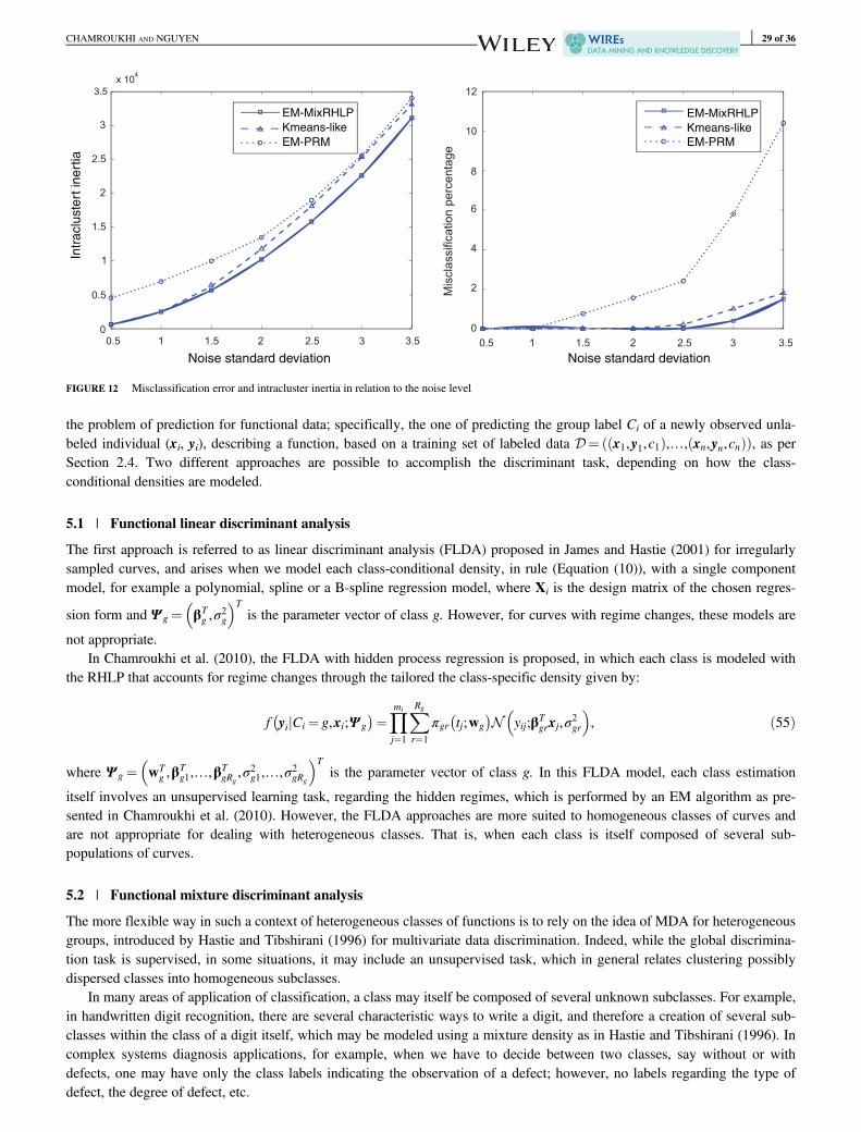
the problem of prediction for functional data; specifically, the one of predicting the group label Ci of a newly observed unla-beled individual (xi, yi), describing a function, based on a training set of labeled data D¼ x1,y1,c1ð Þ,…, xn,yn,cnð Þð Þ, as perSection 2.4. Two different approaches are possible to accomplish the discriminant task, depending on how the class-conditional densities are modeled.

5.1 | Functional linear discriminant analysis

The first approach is referred to as linear discriminant analysis (FLDA) proposed in James and Hastie (2001) for irregularlysampled curves, and arises when we model each class-conditional density, in rule (Equation (10)), with a single componentmodel, for example a polynomial, spline or a B-spline regression model, where Xi is the design matrix of the chosen regres-

sion form and Ψ g ¼ βTg ,σ

2g

� �Tis the parameter vector of class g. However, for curves with regime changes, these models are

not appropriate.In Chamroukhi et al. (2010), the FLDA with hidden process regression is proposed, in which each class is modeled with

the RHLP that accounts for regime changes through the tailored the class-specific density given by:

f yijCi ¼ g,xi;Ψ g� �

¼Ymi

j¼1

XRg

r¼1

πgr tj;wg� �

N yij;βTgrxj,σ

2gr

� �, ð55Þ

where Ψ g ¼ wTg ,β

Tg1,…,βT

gRg,σ2g1,…,σ2gRg

� �Tis the parameter vector of class g. In this FLDA model, each class estimation

itself involves an unsupervised learning task, regarding the hidden regimes, which is performed by an EM algorithm as pre-sented in Chamroukhi et al. (2010). However, the FLDA approaches are more suited to homogeneous classes of curves andare not appropriate for dealing with heterogeneous classes. That is, when each class is itself composed of several sub-populations of curves.

5.2 | Functional mixture discriminant analysis

The more flexible way in such a context of heterogeneous classes of functions is to rely on the idea of MDA for heterogeneousgroups, introduced by Hastie and Tibshirani (1996) for multivariate data discrimination. Indeed, while the global discrimina-tion task is supervised, in some situations, it may include an unsupervised task, which in general relates clustering possiblydispersed classes into homogeneous subclasses.

In many areas of application of classification, a class may itself be composed of several unknown subclasses. For example,in handwritten digit recognition, there are several characteristic ways to write a digit, and therefore a creation of several sub-classes within the class of a digit itself, which may be modeled using a mixture density as in Hastie and Tibshirani (1996). Incomplex systems diagnosis applications, for example, when we have to decide between two classes, say without or withdefects, one may have only the class labels indicating the observation of a defect; however, no labels regarding the type ofdefect, the degree of defect, etc.

EM-MixRHLP

Noise standard deviation Noise standard deviation

Kmeans-like

EM-PRM

EM-MixRHLP

Kmeans-like

EM-PRM

Intr

aclu

ste

rt in

ert

ia

FIGURE 12 Misclassification error and intracluster inertia in relation to the noise level


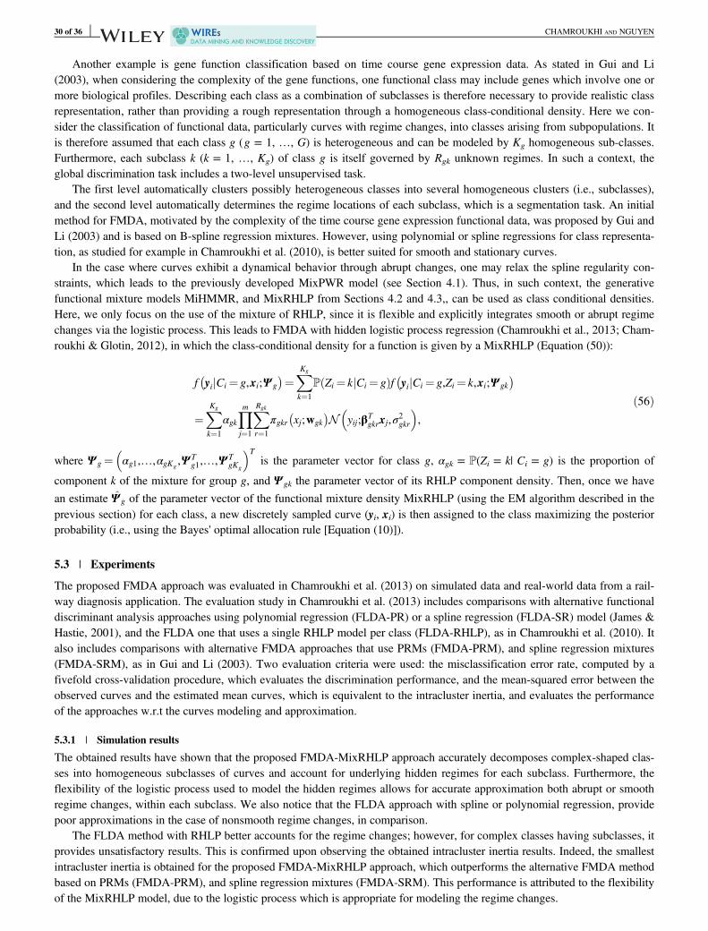
Another example is gene function classification based on time course gene expression data. As stated in Gui and Li(2003), when considering the complexity of the gene functions, one functional class may include genes which involve one ormore biological profiles. Describing each class as a combination of subclasses is therefore necessary to provide realistic classrepresentation, rather than providing a rough representation through a homogeneous class-conditional density. Here we con-sider the classification of functional data, particularly curves with regime changes, into classes arising from subpopulations. Itis therefore assumed that each class g (g = 1, …, G) is heterogeneous and can be modeled by Kg homogeneous sub-classes.Furthermore, each subclass k (k = 1, …, Kg) of class g is itself governed by Rgk unknown regimes. In such a context, theglobal discrimination task includes a two-level unsupervised task.

The first level automatically clusters possibly heterogeneous classes into several homogeneous clusters (i.e., subclasses),and the second level automatically determines the regime locations of each subclass, which is a segmentation task. An initialmethod for FMDA, motivated by the complexity of the time course gene expression functional data, was proposed by Gui andLi (2003) and is based on B-spline regression mixtures. However, using polynomial or spline regressions for class representa-tion, as studied for example in Chamroukhi et al. (2010), is better suited for smooth and stationary curves.

In the case where curves exhibit a dynamical behavior through abrupt changes, one may relax the spline regularity con-straints, which leads to the previously developed MixPWR model (see Section 4.1). Thus, in such context, the generativefunctional mixture models MiHMMR, and MixRHLP from Sections 4.2 and 4.3,, can be used as class conditional densities.Here, we only focus on the use of the mixture of RHLP, since it is flexible and explicitly integrates smooth or abrupt regimechanges via the logistic process. This leads to FMDA with hidden logistic process regression (Chamroukhi et al., 2013; Cham-roukhi & Glotin, 2012), in which the class-conditional density for a function is given by a MixRHLP (Equation (50)):

f yijCi ¼ g,xi;Ψ g� �

¼XKg

k¼1

P Zi ¼ kjCi ¼ gð Þf yijCi ¼ g,Zi ¼ k,xi;Ψ gk� �

¼XKg

k¼1

αgkYmj¼1

XRgk

r¼1

πgkr xj;wgk� �

N yij;βTgkrxj,σ

2gkr

� �,

ð56Þ

where Ψ g ¼ αg1,…,αgKg,Ψ T

g1,…,Ψ TgKg

� �Tis the parameter vector for class g, αgk = P(Zi = k| Ci = g) is the proportion of

component k of the mixture for group g, and Ψ gk the parameter vector of its RHLP component density. Then, once we have

an estimate Ψ g of the parameter vector of the functional mixture density MixRHLP (using the EM algorithm described in theprevious section) for each class, a new discretely sampled curve (yi, xi) is then assigned to the class maximizing the posteriorprobability (i.e., using the Bayes' optimal allocation rule [Equation (10)]).

5.3 | Experiments

The proposed FMDA approach was evaluated in Chamroukhi et al. (2013) on simulated data and real-world data from a rail-way diagnosis application. The evaluation study in Chamroukhi et al. (2013) includes comparisons with alternative functionaldiscriminant analysis approaches using polynomial regression (FLDA-PR) or a spline regression (FLDA-SR) model (James &Hastie, 2001), and the FLDA one that uses a single RHLP model per class (FLDA-RHLP), as in Chamroukhi et al. (2010). Italso includes comparisons with alternative FMDA approaches that use PRMs (FMDA-PRM), and spline regression mixtures(FMDA-SRM), as in Gui and Li (2003). Two evaluation criteria were used: the misclassification error rate, computed by afivefold cross-validation procedure, which evaluates the discrimination performance, and the mean-squared error between theobserved curves and the estimated mean curves, which is equivalent to the intracluster inertia, and evaluates the performanceof the approaches w.r.t the curves modeling and approximation.


The obtained results have shown that the proposed FMDA-MixRHLP approach accurately decomposes complex-shaped clas-ses into homogeneous subclasses of curves and account for underlying hidden regimes for each subclass. Furthermore, theflexibility of the logistic process used to model the hidden regimes allows for accurate approximation both abrupt or smoothregime changes, within each subclass. We also notice that the FLDA approach with spline or polynomial regression, providepoor approximations in the case of nonsmooth regime changes, in comparison.

The FLDA method with RHLP better accounts for the regime changes; however, for complex classes having subclasses, itprovides unsatisfactory results. This is confirmed upon observing the obtained intracluster inertia results. Indeed, the smallestintracluster inertia is obtained for the proposed FMDA-MixRHLP approach, which outperforms the alternative FMDA methodbased on PRMs (FMDA-PRM), and spline regression mixtures (FMDA-SRM). This performance is attributed to the flexibilityof the MixRHLP model, due to the logistic process which is appropriate for modeling the regime changes.


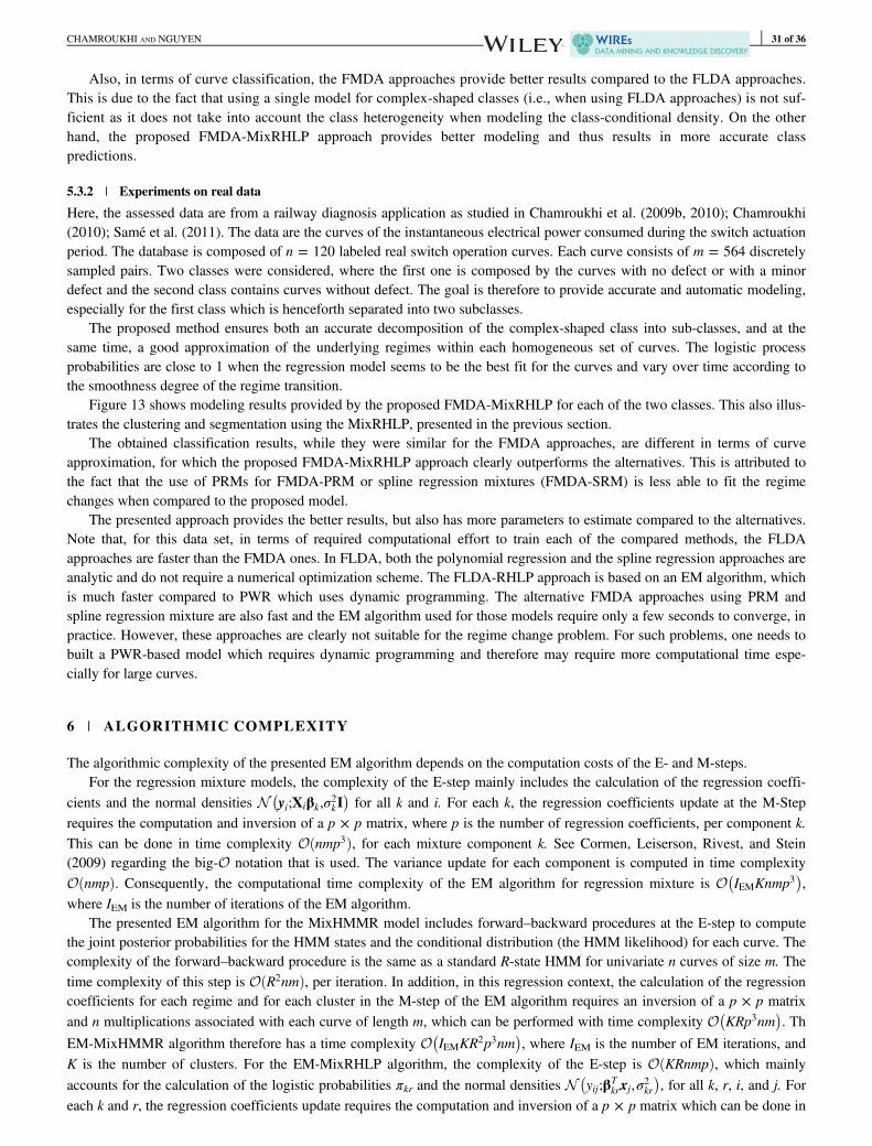
Also, in terms of curve classification, the FMDA approaches provide better results compared to the FLDA approaches.This is due to the fact that using a single model for complex-shaped classes (i.e., when using FLDA approaches) is not suf-ficient as it does not take into account the class heterogeneity when modeling the class-conditional density. On the otherhand, the proposed FMDA-MixRHLP approach provides better modeling and thus results in more accurate classpredictions.

5.3.2 | Experiments on real data

Here, the assessed data are from a railway diagnosis application as studied in Chamroukhi et al. (2009b, 2010); Chamroukhi(2010); Samé et al. (2011). The data are the curves of the instantaneous electrical power consumed during the switch actuationperiod. The database is composed of n = 120 labeled real switch operation curves. Each curve consists of m = 564 discretelysampled pairs. Two classes were considered, where the first one is composed by the curves with no defect or with a minordefect and the second class contains curves without defect. The goal is therefore to provide accurate and automatic modeling,especially for the first class which is henceforth separated into two subclasses.

The proposed method ensures both an accurate decomposition of the complex-shaped class into sub-classes, and at thesame time, a good approximation of the underlying regimes within each homogeneous set of curves. The logistic processprobabilities are close to 1 when the regression model seems to be the best fit for the curves and vary over time according tothe smoothness degree of the regime transition.

Figure 13 shows modeling results provided by the proposed FMDA-MixRHLP for each of the two classes. This also illus-trates the clustering and segmentation using the MixRHLP, presented in the previous section.

The obtained classification results, while they were similar for the FMDA approaches, are different in terms of curveapproximation, for which the proposed FMDA-MixRHLP approach clearly outperforms the alternatives. This is attributed tothe fact that the use of PRMs for FMDA-PRM or spline regression mixtures (FMDA-SRM) is less able to fit the regimechanges when compared to the proposed model.

The presented approach provides the better results, but also has more parameters to estimate compared to the alternatives.Note that, for this data set, in terms of required computational effort to train each of the compared methods, the FLDAapproaches are faster than the FMDA ones. In FLDA, both the polynomial regression and the spline regression approaches areanalytic and do not require a numerical optimization scheme. The FLDA-RHLP approach is based on an EM algorithm, whichis much faster compared to PWR which uses dynamic programming. The alternative FMDA approaches using PRM andspline regression mixture are also fast and the EM algorithm used for those models require only a few seconds to converge, inpractice. However, these approaches are clearly not suitable for the regime change problem. For such problems, one needs tobuilt a PWR-based model which requires dynamic programming and therefore may require more computational time espe-cially for large curves.

6 | ALGORITHMIC COMPLEXITY

The algorithmic complexity of the presented EM algorithm depends on the computation costs of the E- and M-steps.For the regression mixture models, the complexity of the E-step mainly includes the calculation of the regression coeffi-

cients and the normal densities N yi;Xiβk,σ2kI� �

for all k and i. For each k, the regression coefficients update at the M-Steprequires the computation and inversion of a p × p matrix, where p is the number of regression coefficients, per component k.This can be done in time complexity O nmp3ð Þ, for each mixture component k. See Cormen, Leiserson, Rivest, and Stein(2009) regarding the big-O notation that is used. The variance update for each component is computed in time complexityO nmpð Þ. Consequently, the computational time complexity of the EM algorithm for regression mixture is O IEMKnmp3

� �,

where IEM is the number of iterations of the EM algorithm.The presented EM algorithm for the MixHMMR model includes forward–backward procedures at the E-step to compute

the joint posterior probabilities for the HMM states and the conditional distribution (the HMM likelihood) for each curve. Thecomplexity of the forward–backward procedure is the same as a standard R-state HMM for univariate n curves of size m. Thetime complexity of this step is O R2nmð Þ, per iteration. In addition, in this regression context, the calculation of the regressioncoefficients for each regime and for each cluster in the M-step of the EM algorithm requires an inversion of a p × p matrixand n multiplications associated with each curve of length m, which can be performed with time complexity O KRp3nm

� �. Th

EM-MixHMMR algorithm therefore has a time complexity O IEMKR2p3nm� �

, where IEM is the number of EM iterations, andK is the number of clusters. For the EM-MixRHLP algorithm, the complexity of the E-step is O KRnmpð Þ, which mainlyaccounts for the calculation of the logistic probabilities πkr and the normal densities N yij;βT

krxj,σ2kr

� �, for all k, r, i, and j. For

each k and r, the regression coefficients update requires the computation and inversion of a p × p matrix which can be done in


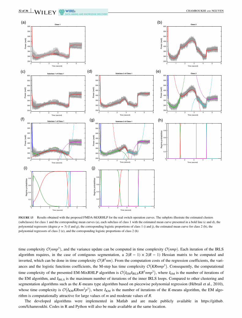
time complexity O nmp3ð Þ, and the variance update can be computed in time complexity O nmpð Þ. Each iteration of the IRLSalgorithm requires, in the case of contiguous segmentation, a 2(R − 1) × 2(R − 1) Hessian matrix to be computed andinverted, which can be done in time complexity O R3nmð Þ. From the computation costs of the regression coefficients, the vari-ances and the logistic functions coefficients, the M-step has time complexity O KRnmp3

� �. Consequently, the computational

time complexity of the presented EM-MixRHLP algorithm is O IEMIIRLSKR3nmp3� �

, where IEM is the number of iterations ofthe EM algorithm, and IIRLS is the maximum number of iterations of the inner IRLS loops. Compared to other clustering andsegmentation algorithms such as the K-means type algorithm based on piecewise polynomial regression (Hébrail et al., 2010),whose time complexity is O IKMKRnm2p3

� �, where IKM is the number of iterations of the K-means algorithm, the EM algo-

rithm is computationally attractive for large values of m and moderate values of R.The developed algorithms were implemented in Matlab and are made publicly available in https://github.

com/fchamroukhi. Codes in R and Python will also be made available at the same location.

0 1 2 3 4 5 6

250

300

350

400

450

500

550

600

Time (second)

Po

we

r (w

att

)Class 1

(a)

0 1 2 3 4 5 6

250

300

350

400

450

500

550

600

Time (second)

Po

we

r (w

att

)

Class 2(b)

0 1 2 3 4 5 6

250

300

350

400

450

500

550

600

Time (second)

Po

we

r (w

att

)

Subclass 1 of Class 1(c)

0 1 2 3 4 5 6

250

300

350

400

450

500

550

600

Time (second)

Po

we

r (w

att

)

Subclass 2 of Class 1(d)

0 1 2 3 4 5 6

250

300

350

400

450

500

550

600

Time (second)

Po

we

r (w

att

)

Class 2(e)

0 1 2 3 4 5 6

250

300

350

400

450

500

550

600

Time (second)

Po

we

r (w

att

)

Subclass 1 of Class 1(f)

0 1 2 3 4 5 6

250

300

350

400

450

500

550

600

Time (second)

Po

we

r (w

att

)

Subclass 2 of Class 1(g)

0 1 2 3 4 5 60

0.2

0.4

0.6

0.8

1

Time (second)R

egim

e p

robabili

ties

(h)

0 1 2 3 4 5 60

0.2

0.4

0.6

0.8

1

Time (second)

Regim

e p

robabili

ties

(i)

0 1 2 3 4 5 60

0.2

0.4

0.6

0.8

1

Time (second)

Regim

e p

robabili

ties

(j)

FIGURE 13 Results obtained with the proposed FMDA-MiXRHLP for the real switch operation curves. The subplots illustrate the estimated clusters(subclasses) for class 1 and the corresponding mean curves (a), each subclass of class 1 with the estimated mean curve presented in a bold line (c and d), thepolynomial regressors (degree p = 3) (f and g), the corresponding logistic proportions of class 1 (i and j), the estimated mean curve for class 2 (b), thepolynomial regressors of class 2 (e), and the corresponding logistic proportions of class 2 (h)


https://github.com/fchamroukhi

https://github.com/fchamroukhi

7 | CONLUSIONS

FDA is an important topic in statistics. Latent data modeling is a powerful paradigm for the analysis of complex data withunknown hidden structures, and thus for the cluster and the discriminant analyses of heterogeneous data. We presented mix-ture model-based approaches and demonstrated the inferential capabilities of such models for the analysis of functional data.We demonstrated how clustering, classification, and regression could be conducted, in such situations.

We studied the regression mixtures and presented a new robust EM-like algorithm for fitting regression mixtures andmodel-based curve clustering. The approach optimizes a penalized log-likelihood and overcomes both the problems of sensi-tivity to initialization and uncertainty of the number of clusters in standard EM algorithms for regression mixtures. This consti-tutes an interesting fully unsupervised approach that simultaneously infers the model and its optimal number of components.We also considered the problem of modeling and clustering of spatial functional data, using dedicated regression mixturemodel with mixed-effects. The experimental results on simulated data and real-world data demonstrate the benefit of the pro-posed approach for applications in curve and surface clustering.

We then studied the problem of simultaneous clustering and segmentation of functions governed by regime changes. Weintroduced a new probabilistic approach, based on a PWRM for simultaneous clustering and optimal segmentation of curveswith regime changes. We provided two algorithms for parameter estimation. The first (EM-PWRM) consists of using the EMalgorithm to maximize the observed data log-likelihood and the latter (CEM-PWRM) is a CEM algorithm to maximize thecomplete-data log-likelihood. We showed that the CEM-PWRM algorithm is a probabilistic generalization of the K-means-like algorithm of Hébrail et al. (2010). However, it is worth mentioning that if the aim is density estimation, the EM version issuggested since the CEM provides biased estimators but is suitable for segmentation and clustering. The obtained results dem-onstrated the benefits of the proposed approaches in terms of both curve clustering, and piecewise approximation and segmen-tation of the regimes of each cluster. In particular, the comparisons with the K-means-like algorithm approach confirm that theproposed CEM-PWRM is an interesting probabilistic alternative.

We note that in some practical situations involving continuous functions the proposed PWRM, in its current formulation,may lead to discontinuities between segments for the piecewise approximation. This may be avoided by slightly modifyingthe algorithm by adding an interpolation step as performed in Hébrail et al. (2010).

The introduced mixture of polynomial regression models, governed by hidden Markov chains, is particularly appropriatefor clustering curves with various changes in regime and that rely on a suitable generative formulation. The experimentalresults demonstrated the benefit of the proposed approach as compared to existing methods, including the regression mixturemodel and the standard mixture of hidden Markov models. It also represents a fully generative alternative to the previouslydescribed mixture of PWRs. While the model in its current form only concerns univariate time series, we believe that its exten-sion to the multivariate case is immediately possible.

We then presented a new mixture model-based approach for clustering and segmentation of univariate functional data,with changes in regime. This approach involves modeling each cluster using a particular regression model whose polynomialcoefficients vary across the range of the inputs, typically time, according to a discrete hidden process. The transition betweenregimes is smoothly controlled by logistic functions. The maximum likelihood estimate of the model parameter is conductedvia a dedicated EM algorithm. The proposed approach can also be regarded as a clustering approach, which operates by find-ing groups of time series having common changes in regime. The experimental results, both from simulated time series andfrom a real-world application, show that the proposed approach is an efficient means for clustering univariate time series withchanges in regime.

Note that a CEM derivation of the current version immediately possible, and consists of assigning the curves in a hardway during the EM iterations. One can further extend this to the regimes, by assigning the observations to the regimes also ina hard way, especially in the case, where there are only abrupt change points in order to promote the segmentation.

Finally, the presented mixture model-based approach for functional data discrimination includes unsupervised tasks thatrelate clustering heterogeneous classes and determining possible underlying unknown regimes for each subclass. It is suitablefor the classification of curves, organized in subgroups, and presenting a nonstationary behavior arising in regime changes.Furthermore, the proposed functional discriminant analysis approach, as it uses a hidden logistic process regression model foreach class, is particularly suitable for modeling abrupt or smooth regime changes. Each class is trained in an unsupervisedway by a dedicated EM algorithm.

ACKNOWLEDGMENTS

The authors would like to very much thank the anonymous reviewers and the editor for their very helpful comments whohelped to improve the manuscript. Faicel Chamroukhi is supported by ANR via the grant SMILES ANR-18-CE40-0014 and


the Région Normandie via the grant RIN AStERiCs. Hien Nguyen is funded by Australian Research Council grantsDE170101134 and DP180101192.

CONFLICT OF INTEREST

The authors have declared no conflicts of interest for this article.

ENDNOTES1Phonemes data from http://www.math.univ-toulouse.fr/staph/npfda/ is a part of the original one available at http://www-stat.stanford.edu/ElemStatLearn.2Tecator data are available at http://lib.stat.cmu.edu/datasets/tecator.3We consider the standardized subset constructed by Yeung et al. (2001) available in http://faculty.washington.edu/kayee/model/. The complete data are available from http://genome-www.stanford.edu/cellcycle/.4Satellite data are available at http://www.lsp.ups-tlse.fr/staph/npfda/npfda-datasets.html.5Data from http://www.math.univ-toulouse.fr/staph/npfda/6The complete data are from http://genome-www.stanford.edu/cellcycle/.7The adjusted Rand index measures the similarity between two data clusterings, and consists of a randomness adjusted modifi-cation of the index of Rand (1971). It was first proposed by Hubert and Arabie (1985) and has an optimal value of 1 (withhigher values indicating better correspondence between labelings).

RELATED WIREs ARTICLES

Practical and theoretical aspects of mixture-of-experts modeling: An overview

ORCID

Faicel Chamroukhi https://orcid.org/0000-0002-5894-3103

Hien D. Nguyen https://orcid.org/0000-0002-9958-432X

REFERENCES

Abraham, C., Cornillon, P. A., Matzner-Lober, E., & Molinari, N. (2003). Unsupervised curve clustering using B-splines. Scandinavian Journal of Statistics, 30(3), 581–595.Akaike, H. (1974). A new look at the statistical model identification. IEEE Transactions on Automatic Control, 19(6), 716–723.Alon, J., Sclaroff, S., Kollios, G., & Pavlovic, V. (2003). Discovering clusters in motion time-series data. Paper presented at the Proceedings of the 2003 I.E. Computer

Society Conference on Computer Vision and Pattern Recognition (CVPR) (pp. 375–381), Los Alamitos, CA.Antoniadis, A., Brossat, X., Cugliari, J., & Poggi, J.-M. (2013). Functional clustering using wavelets. International Journal of Wavelets, Multiresolution and Informa-

tion Processing, 11(1). Retrieved from https://www.worldscientific.com/doi/10.1142/S0219691313500033Baudry, J.-P. (2015). Estimation and model selection for model-based clustering with the conditional classification likelihood. Electronic Journal of Statistics, 9(1),

1041–1077.Bensmail, H., Celeux, G., Raftery, A. E., & Robert, C. P. (1997). Inference in model-based cluster analysis. Statistics and Computing, 7(1), 1–10.Biernacki, C., Celeux, G., & Govaert, G. (2000). Assessing a mixture model for clustering with the integrated completed likelihood. IEEE Transactions on Pattern

Analysis and Machine Intelligence, 22(7), 719–725.Biernacki, C., Celeux, G., & Govaert, G. (2003). Choosing starting values for the EM algorithm for getting the highest likelihood in multivariate gaussian mixture

models. Computational Statistics and Data Analysis, 41, 561–575.Bouveyron, C., & Jacques, J. (2011). Model-based clustering of time series in group-specific functional subspaces. Advances in Data Analysis and Classification, 5(4),

281–300.Breiman, L., Friedman, J. H., Olshen, R. A., & Stone, C. J. (1984). Classification and regression trees. New York: Wadsworth.Celeux, G., & Diebolt, J. (1985). The SEM algorithm a probabilistic teacher algorithm derived from the EM algorithm for the mixture problem. Computational Statistics

Quarterly, 2(1), 73–82.Celeux, G., & Govaert, G. (1992). A classification EM algorithm for clustering and two stochastic versions. Computational Statistics and Data Analysis, 14, 315–332.Celeux, G., Martin, O., & Lavergne, C. (2005). Mixture of linear mixed models for clustering gene expression profiles from repeated microarray experiments. Statistical

Modelling, 5, 1–25.Chamroukhi, F. (2010). Hidden process regression for curve modeling, classification and tracking. (Ph.D. thesis). Université de Technologie de Compiègne.Chamroukhi, F. (2013). Robust EM algorithm for model-based curve clustering. Paper presented at the Proceedings of the International Joint Conference on Neural Net-

works (IJCNN) (pp. 1–8), IEEE, Dallas, TX.Chamroukhi, F. (2015a). Bayesian mixtures of spatial spline regressions. arXiv:1508.00635.Chamroukhi, F. (2015b). Statistical learning of latent data models for complex data analysis. (Accreditation to Supervise Research Thesis (HDR)), Université de Toulon.Chamroukhi, F. (2016a). Piecewise regression mixture for simultaneous functional data clustering and optimal segmentation. Journal of Classification, 33(3), 374–411.Chamroukhi, F. (2016b). Unsupervised learning of regression mixture models with unknown number of components. Journal of Statistical Computation and Simulation,

86, 2308–2334.


http://www.math.univ-toulouse.fr/staph/npfda/

http://www-stat.stanford.edu/ElemStatLearn

http://www-stat.stanford.edu/ElemStatLearn

http://lib.stat.cmu.edu/datasets/tecator



http://genome-www.stanford.edu/cellcycle/

http://www.lsp.ups-tlse.fr/staph/npfda/npfda-datasets.html

http://www.math.univ-toulouse.fr/staph/npfda/

http://genome-www.stanford.edu/cellcycle/


https://orcid.org/0000-0002-5894-3103

https://orcid.org/0000-0002-5894-3103

https://orcid.org/0000-0002-9958-432X

https://orcid.org/0000-0002-9958-432X

https://www.worldscientific.com/doi/10.1142/S0219691313500033

Chamroukhi, F. & Glotin, H. (2012). Mixture model-based functional discriminant analysis for curve classification. Paper presented at the Proceedings of the Interna-tional Joint Conference on Neural Networks (IJCNN) (1–8), IEEE, Brisbane, Australia.

Chamroukhi, F., Glotin, H., & Samé, A. (2013). Model-based functional mixture discriminant analysis with hidden process regression for curve classification. Neuro-computing, 112, 153–163.

Chamroukhi, F., Samé, A., Aknin, P., & Govaert, G. (2011). Model-based clustering with hidden markov model regression for time series with regime changes. Paperpresented at the Proceedings of the International Joint Conference on Neural Networks (IJCNN) (pp. 2814–2821), IEEE, San Jose, California.

Chamroukhi, F., Samé, A., Govaert, G., & Aknin, P. (2009a). A regression model with a hidden logistic process for feature extraction from time series. Paper presentedat the International Joint Conference on Neural Networks (IJCNN) (pp. 489–496), Atlanta, GA.

Chamroukhi, F., Samé, A., Govaert, G., & Aknin, P. (2009b). Time series modeling by a regression approach based on a latent process. Neural Networks, 22(5–6), 593–602.Chamroukhi, F., Samé, A., Govaert, G., & Aknin, P. (2010). A hidden process regression model for functional data description. Application to curve discrimination.

Neurocomputing, 73(7–9), 1210–1221.Cho, R. J., Campbell, M. J., Winzeler, E. A., Steinmetz, L., Conway, A., Wodicka, L., … Davis, R. W. (1998). A genome-wide transcriptional analysis of the mitotic

cell cycle. Molecular Cell, 2(1), 65–73.Cormen, T. H., Leiserson, C. E., Rivest, R. L., & Stein, C. (2009). Introduction to algorithms (3rd ed.). Cambridge, Massachusetts: MIT Press.Dabo-Niang, S., Ferraty, F., & Vieu, P. (2007). On the using of modal curves for radar waveforms classification. Computational Statistics & Data Analysis, 51(10),

4878–4890.de Boor, C. (1978). A practical guide to splines. Berlin: Springer-Verlag.Delaigle, A., Hall, P., & Bathia, N. (2012). Componentwise classification and clustering of functional data. Biometrika, 99(2), 299–313.Dempster, A. P., Laird, N. M., & Rubin, D. B. (1977). Maximum likelihood from incomplete data via the EM algorithm. Journal of The Royal Statistical Society, Series

B, 39(1), 1–38.DeSarbo, W., & Cron, W. (1988). A maximum likelihood methodology for clusterwise linear regression. Journal of Classification, 5(2), 249–282.Devijver, E. (2014). Model-based clustering for high-dimensional data. Application to functional data (Technical Report No. hal-01060063). Département de Mathéma-

tiques, Université Paris-Sud.Diebold, F., Lee, J.-H., & Weinbach, G. (1994). Regime switching with time-varying transition probabilities. In C. Hargreaves (Ed.), Nonstationary Time Series Analy-

sis and Cointegration Advanced Texts in Econometrics (pp. 283–302). Oxford, England: Oxford University Press.Faria, S., & Soromenho, G. (2010). Fitting mixtures of linear regressions. Journal of Statistical Computation and Simulation, 80(2), 201–225.Ferraty, F., & Vieu, P. (2003). Curves discrimination: A nonparametric functional approach. Computational Statistics & Data Analysis, 44(1–2), 161–173.Ferraty, F., & Vieu, P. (2006). Nonparametric functional data analysis: Theory and practice Springer series in statistics (). Springer-Verlag Berlin, Heidelberg: Springer.Figueiredo, M. A. T., & Jain, A. K. (2000). Unsupervised learning of finite mixture models. IEEE Transactions Pattern Analysis and Machine Intelligence, 24, 381–396.Fraley, C. & Raftery, A. E. (2005). Bayesian regularization for normal mixture estimation and model-based clustering (Technical Report No. 486). Seattle, WA, Depar-

tament of Statistics, University of Washington Seattle.Fraley, C., & Raftery, A. E. (2007). Bayesian regularization for normal mixture estimation and model-based clustering. Journal of Classification, 24(2), 155–181.Frühwirth-Schnatter, S. (2006). Finite mixture and Markov switching models Springer Series in Statistics (). New York: Springer Verlag.Gaffney, S. & Smyth, P. (1999). Trajectory clustering with mixtures of regression models. Paper presented at the Proceedings of the fifth ACM SIGKDD international

conference on Knowledge discovery and data mining (pp. 63–72), ACM Press.Gaffney, S. J. (2004). Probabilistic Curve-Aligned Clustering and Prediction with Regression Mixture Models. (Ph.D. Thesis), Department of Computer Science, Uni-

versity of California, Irvine.Gaffney, S. J. & Smyth, P. (2004). Joint probabilistic curve clustering and alignment. Paper presented at the Advances in Neural Information Processing Systems

(NIPS), Vancouver, BC.Giacofci, M., Lambert-Lacroix, S., Marot, G., & Picard, F. (2013). Wavelet-based clustering for mixed-effects functional models in high dimension. Biometrics, 69(1),

31–40.Gui, J. & Li, H. (2003). Mixture functional discriminant analysis for gene function classification based on time course gene expression data. Paper presented at the Pro-

ceedings of the Joint Statistical Meeting (Biometric Section).Hastie, T., Buja, A., & Tibshirani, R. (1995). Penalized discriminant analysis. Annals of Statistics, 23, 73–102.Hastie, T., & Tibshirani, R. (1996). Discriminant analysis by gaussian mixtures. Journal of the Royal Statistical Society, Series B, 58, 155–176.Hastie, T., Tibshirani, R., & Friedman, J. (2010). The elements of statistical learning. In Data mining, inference, and prediction Springer series in statistics (2nd ed.).

New York: Springer.Hébrail, G., Hugueney, B., Lechevallier, Y., & Rossi, F. (2010). Exploratory analysis of functional data via clustering and optimal segmentation. Neurocomputing,

73(7–9), 1125–1141.Hubert, L., & Arabie, P. (1985). Comparing partitions. Journal of Classification, 2(1), 193–218.Hughes, J. P., Guttorp, P., & Charles, S. P. (1999). A non-homogeneous hidden Markov model for precipitation occurrence. Applied Statistics, 48, 15–30.Hunter, D., & Young, D. (2012). Semiparametric mixtures of regressions. Journal of Nonparametric Statistics, 24(1), 19–38.Hunter, D. R., & Lange, K. (2004). A tutorial on MM algorithms. The American Statistician, 58(1), 30–37.Jacques, J., & Preda, C. (2014). Model-based clustering for multivariate functional data. Computational Statistics & Data Analysis, 71, 92–106.James, G. M., & Hastie, T. J. (2001). Functional linear discriminant analysis for irregularly sampled curves. Journal of the Royal Statistical Society, Series B, 63, 533–550.James, G. M., & Sugar, C. (2003). Clustering for sparsely sampled functional data. Journal of the American Statistical Association, 98(462), 397–408.Jones, P. N., & McLachlan, G. J. (1992). Fitting finite mixture models in a regression context. The Australian Journal of Statistics, 34(2), 233–240.Kooperberg, C., & Stone, C. J. (1991). A study of logspline density estimation. Computational Statistics & Data Analysis, 12(3), 327–347.Laird, N. M., & Ware, J. H. (1982). Random-effects models for longitudinal data. Biometrics, 38(4), 963–974.LeCun, Y., Bottou, L., Bengio, Y., & Haffner, P. (1998). Gradient-based learning applied to document recognition. Proceedings of the IEEE, 86(11), 2278–2324.Lenk, P., & DeSarbo, W. (2000). Bayesian inference for finite mixtures of generalized linear models with random effects. Psychometrika, 65(1), 93–119.Liu, X., & Yang, M. (2009). Simultaneous curve registration and clustering for functional data. Computational Statistics and Data Analysis, 53(4), 1361–1376.Malfait, N., & Ramsay, J. O. (2003). The historical functional linear model. The Canadian Journal of Statistics, 31(2), 115–128.Marin, J.-M., Mengersen, K. L., & Robert, C. (2005). Bayesian modelling and inference on mixtures of distributions. In D. Dey & C. Rao (Eds.), Handbook of statistics

(Vol. 25). Amsterdam: Elsevier.McLachlan, G. J. (1982). The classification and mixture maximum likelihood approaches to cluster analysis. In P. Krishnaiah & L. Kanal (Eds.), Handbook of Statistics

(Vol. 2, pp. 199–208). Amsterdam, The Netherlands: North-Holland.McLachlan, G. J., & Krishnan, T. (2008). The EM algorithm and extensions (2nd ed.). New York: Wiley.McLachlan, G. J., & Peel, D. (2000). Finite mixture models. New York: Wiley.Neal, R. M. (1993). Probabilistic inference using Markov Chain Monte Carlo methods (Technical Report No. CRG-TR-93-1). Department of Computer Science, Uni-

versity of Toronto.


Ng, S. K., McLachlan, G. J., Ben-Tovim Jones, L., Wang, K., & Ng, S.-W. (2006). A mixture model with random-effects components for clustering correlated gene-expression profiles. Bioinformatics, 22(14), 1745–1752.

Nguyen, H. D. (2017). An introduction to Majorization-Minimization algorithms for machine learning and statistical estimation. WIREs Data Mining and KnowledgeDiscovery, 7(2), e1198.

Nguyen, H. D., & Chamroukhi, F. (2018). Practical and theoretical aspects of mixture-of-experts modeling: An overview. WIREs Data Mining and Knowledge Discov-ery, 8(4), e1246.

Nguyen, H. D., Lloyd-Jones, L. R., & McLachlan, G. J. (2016). A universal approximation theorem for mixture-of-experts models. Neural Computation, 28(12),2585–2593.

Nguyen, H. D., McLachlan, G. J., Ullmann, J. F. P., & Janke, A. L. (2016). Spatial clustering of time series via mixture of autoregressions models and markov randomfields. Statistica Neerlandica, 70(4), 414–439.

Nguyen, H. D., McLachlan, G. J., & Wood, I. A. (2016). Mixtures of spatial spline regressions for clustering and classification. Computational Statistics & Data Analy-sis, 93, 76–85.

Nguyen, H. D., Ullmann, J. F. P., McLachlan, G. J., Voleti, V., Li, W., Hillman, E. M. C., … Janke, A. L. (2018). Whole-volume clustering of time series data fromzebrafish brain calcium images via mixture modeling. Statistical Analysis and Data Mining, 11(1), 5–16.

Quandt, R. E. (1972). A new approach to estimating switching regressions. Journal of the American Statistical Association, 67(338), 306–310.Quandt, R. E., & Ramsey, J. B. (1978). Estimating mixtures of normal distributions and switching regressions. Journal of the American Statistical Association, 73(364), 730–738.Rabiner, L. R. (1989). A tutorial on hidden Markov models and selected applications in speech recognition. Proceedings of the IEEE, 77(2), 257–286.Rabiner, L. R., & Juang, B. H. (1986). An introduction to hidden Markov models. IEEE ASSP Magazine, 3(1), 4–16.Raftery, A. E., & Lewis, S. (1992). How many iterations in the Gibbs sampler? Bayesian Statistics, 4, 763–773.Ramsay, J., Ramsay, T., & Sangalli, L. (2011). Spatial functional data analysis. In F. Ferraty (Ed.), Recent advances in functional data analysis and related topics

(pp. 269–275). Berlin: Springer.Ramsay, J. O., & Silverman, B. W. (2002). Applied functional data analysis: Methods and case studies (Springer series in statistics). Berlin: Springer.Ramsay, J. O., & Silverman, B. W. (2005). Functional data analysis (Springer series in statistics). New York: Springer.Rand, W. (1971). Objective criteria for the evaluation of clustering methods. Journal of the American Statistical Association, 66(336), 846–850.Reddy, C. K., Chiang, H.-D., & Rajaratnam, B. (2008). Trust-tech-based expectation maximization for learning finite mixture models. IEEE Transactions on Pattern

Analysis and Machine Intelligence, 30(7), 1146–1157.Richardson, S., & Green, P. J. (1997). On bayesian analysis of mixtures with an unknown number of components. Journal of the Royal Statistical Society, 59(4), 731–792.Robert, C., & Casella, G. (2011). A short history of Markov chain Monte Carlo: Subjective recollections from incomplete data. Statistical Science, 26(1), 102–115.Ruppert, D., Wand, M., & Carroll, R. (2003). Semiparametric regression. Cambridge, Massachusetts: Cambridge University Press.Samé, A., Chamroukhi, F., Govaert, G., & Aknin, P. (2011). Model-based clustering and segmentation of time series with changes in regime. Advances in Data Analysis

and Classification, 5, 301–321.Sangalli, L., Ramsay, J., & Ramsay, T. (2013). Spatial spline regression models. Journal of the Royal Statistical Society, Series B, 75, 681–703.Schwarz, G. (1978). Estimating the dimension of a model. Annals of Statistics, 6, 461–464.Scott, A. J., & Symons, M. J. (1971). Clustering methods based on likelihood ratio criteria. Biometrics, 27, 387–397.Scrucca, L., Fop, M., Murphy, T. B., & Raftery, A. E. (2016). mclust 5: Clustering, classification and density estimation using gaussian finite mixture models. The R

Journal, 8(1), 289–317.Shi, J. Q., & Choi, T. (2011). Gaussian process regression analysis for functional data. Boca Raton, FL: Chapman & Hall/CRC Press.Shi, J. Q., Murray-Smith, R., & Titterington, D. M. (2005). Hierarchical gaussian process mixtures for regression. Statistics and Computing, 15(1), 31–41.Shi, J. Q., & Wang, B. (2008). Curve prediction and clustering with mixtures of gaussian process functional regression models. Statistics and Computing, 18(3), 267–283.Smyth, P. (1996). Clustering sequences with hidden markov models. Paper presented at the Advances in Neural Information Processing Systems (pp. 648–654), 9, NIPS.Snoussi, H. & Mohammad-Djafari, A. (2002). Penalized maximum likelihood for multivariate Gaussian mixture., In R. L. Fry (Ed.), Bayesian Inference and Maximum

Entropy Methods (pp. 36 -46). College Park, Maryland: American Institute of Physics.Snoussi, H. & Mohammad-Djafari, A. (2005). Degeneracy and likelihood penalization in multivariate gaussian mixture models. Technical report, ISTIT/M2S, Univer-

sity of Technology of Troyes.Stephens, M. (1997). Bayesian methods for mixtures of normal distributions. (Ph.D. thesis), University of Oxford.Titterington, D., Smith, A., & Makov, U. (1985). Statistical analysis of finite mixture distributions. Hoboken, New Jersey: John Wiley & Sons.Trabelsi, D., Mohammed, S., Chamroukhi, F., Oukhellou, L., & Amirat, Y. (2013). An unsupervised approach for automatic activity recognition based on hidden mar-

kov model regression. IEEE Transactions on Automation Science and Engineering, 10(3), 829–335.Veaux, R. D. D. (1989). Mixtures of linear regressions. Computational Statistics and Data Analysis, 8(3), 227–245.Verbeke, G., & Lesaffre, E. (1996). A linear mixed-effects model with heterogeneity in the random-effects population. Journal of the American Statistical Association,

91(433), 217–221.Viele, K., & Tong, B. (2002). Modeling with mixtures of linear regressions. Statistics and Computing, 12, 315–330.Wang, K., Ng, S., & McLachlan, G. J. (2009). Multivariate skew t mixture models: Applications to fluorescence-activated cell sorting data. Paper presented at the 2009

Digital Image Computing: Techniques and Applications (pp. 526–531), Melbourne, Australia.Wu, C. F. J. (1983). On the convergence properties of the EM algorithm. The Annals of Statistics, 11(1), 95–103.Xiong, Y., & Yeung, D.-Y. (2004). Time series clustering with ARMA mixtures. Pattern Recognition, 37(8), 1675–1689.Xu, W., & Hedeker, D. (2001). A random-effects mixture model for classifying treatment response in longitudinal clinical trials. Journal of Biopharmaceutical Statis-

tics, 11(4), 253–273.Yang, M.-S., Lai, C.-Y., & Lin, C.-Y. (2012). A robust EM clustering algorithm for Gaussian mixture models. Pattern Recognition, 45(11), 3950–3961.Yeung, K. Y., Fraley, C., Murua, A., Raftery, A. E., & Ruzzo, W. L. (2001). Model-based clustering and data transformations for gene expression data. Bioinformatics,

17(10), 977–987.Young, D., & Hunter, D. (2010). Mixtures of regressions with predictor-dependent mixing proportions. Computational Statistics and Data Analysis, 55(10),

2253–2266.

How to cite this article: Chamroukhi F, Nguyen HD. Model-based clustering and classification of functional data.WIREs Data Mining Knowl Discov. 2019;e1298. https://doi.org/10.1002/widm.1298



Documents

Model-Based Clustering and Classification of Functional Data · approaches for model-based clustering and classification of functional data. We present well-grounded statistical models