Model-based analysis of disease states of the brain using generative embedding

Kay H. Brodersen1,2

1 Translational Neuromodeling Unit (TNU), Department of Biomedical Engineering, University of Zurich & ETH Zurich 2 Machine Learning Laboratory, Department of Computer Science, ETH Zurich

2

Schizophrenia, depression, mania, etc.

genetically based diagnoses impossible (diverse genetic basis, strong gene-environment interactions)

even when symptoms are similar, causes can differ across patients (multiple pathophysiological mechanisms)

large variability in treatment response

Psychiatric spectrum diseases

Consequences need to infer on pathophysiological mechanisms in individual patients!

3

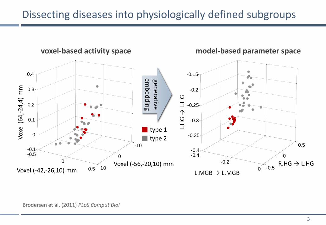
Dissecting diseases into physiologically defined subgroups

-10

0

10

-0.5

0

0.5

-0.1

0

0.1

0.2

0.3

0.4

-0.4

-0.2

0 -0.5

0

0.5-0.4

-0.35

-0.3

-0.25

-0.2

-0.15

-10

0

10

-0.5

0

0.5

-0.1

0

0.1

0.2

0.3

0.4

-0.4

-0.2

0 -0.5

0

0.5-0.4

-0.35

-0.3

-0.25

-0.2

-0.15generative

emb

ed

din

g L.

HG

→ L

.HG

Vo

xel (

64

,-2

4,4

) m

m

L.MGB → L.MGB Voxel (-42,-26,10) mm Voxel (-56,-20,10) mm R.HG → L.HG

type 2

type 1

voxel-based activity space model-based parameter space

Brodersen et al. (2011) PLoS Comput Biol

4

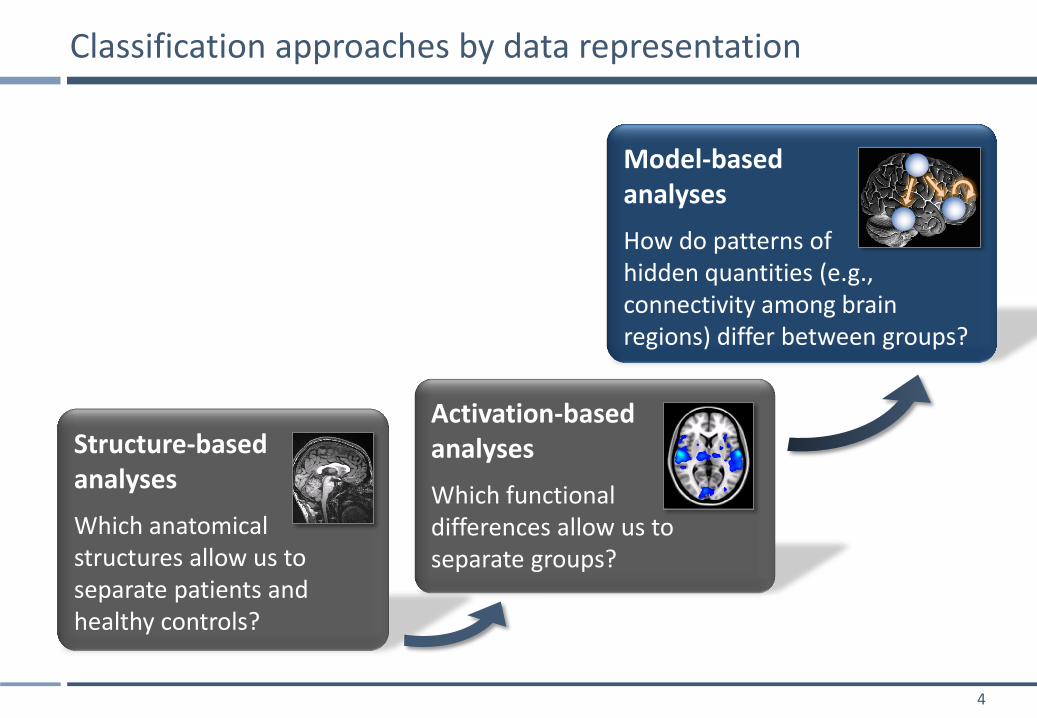
Model-based analyses

How do patterns of hidden quantities (e.g., connectivity among brain regions) differ between groups?

Classification approaches by data representation

Structure-based analyses

Which anatomical structures allow us to separate patients and healthy controls?

Activation-based analyses

Which functional differences allow us to separate groups?

5

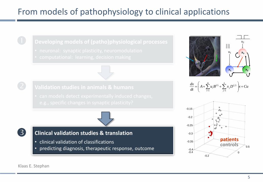
From models of pathophysiology to clinical applications

Developing models of (patho)physiological processes

• neuronal: synaptic plasticity, neuromodulation • computational: learning, decision making

Validation studies in animals & humans

• can models detect experimentally induced changes, e.g., specific changes in synaptic plasticity?

Clinical validation studies & translation

• clinical validation of classifications • predicting diagnosis, therapeutic response, outcome

x1 x2

x3

CuxDxBuAdt

dx n

j

j

j

m

i

i

i

1

)(

1

)(

u1

u2

-10

0

10

-0.5

0

0.5

-0.1

0

0.1

0.2

0.3

0.4

-0.4

-0.2

0 -0.5

0

0.5-0.4

-0.35

-0.3

-0.25

-0.2

-0.15

-10

0

10

-0.5

0

0.5

-0.1

0

0.1

0.2

0.3

0.4

-0.4

-0.2

0 -0.5

0

0.5-0.4

-0.35

-0.3

-0.25

-0.2

-0.15

gen

era

tive

em

bed

din

g

L.H

G

L.H

G

Vo

xel (

64,-

24,4

) m

m

L.MGB L.MGBVoxel (-42,-26,10) mm

Voxel (-56,-20,10) mm R.HG L.HG

controlspatients

Voxel-based feature space Generative score space

patients controls

Klaas E. Stephan

6

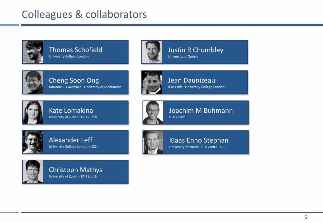
Colleagues & collaborators

Joachim M Buhmann ETH Zurich

Klaas Enno Stephan University of Zurich · ETH Zurich · UCL

Kate Lomakina University of Zurich · ETH Zurich

Alexander Leff University College London (UCL)

Cheng Soon Ong National ICT Australia · University of Melbourne

Thomas Schofield University College London

Justin R Chumbley University of Zurich

Jean Daunizeau ICM Paris · University College London

Christoph Mathys University of Zurich · ETH Zurich

7

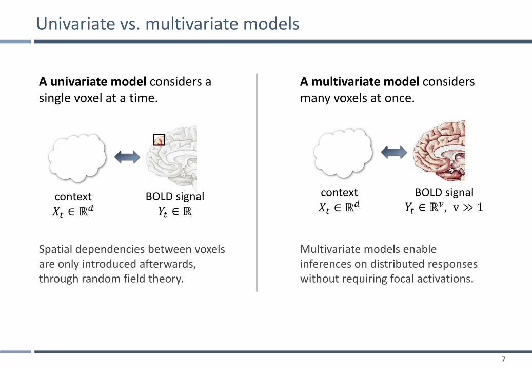
Univariate vs. multivariate models

BOLD signal 𝑌𝑡 ∈ ℝ𝑣, v ≫ 1

context 𝑋𝑡 ∈ ℝ𝑑

A univariate model considers a single voxel at a time.

A multivariate model considers many voxels at once.

Spatial dependencies between voxels are only introduced afterwards, through random field theory.

BOLD signal 𝑌𝑡 ∈ ℝ

context 𝑋𝑡 ∈ ℝ𝑑

Multivariate models enable inferences on distributed responses without requiring focal activations.

8

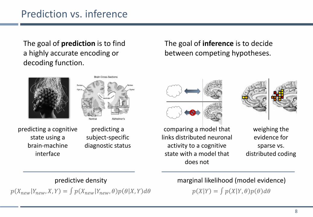
Prediction vs. inference

The goal of prediction is to find a highly accurate encoding or decoding function.

The goal of inference is to decide between competing hypotheses.

predicting a cognitive state using a

brain-machine interface

predicting a subject-specific

diagnostic status

predictive density

𝑝 𝑋𝑛𝑒𝑤 𝑌𝑛𝑒𝑤 , 𝑋, 𝑌 = ∫ 𝑝 𝑋𝑛𝑒𝑤 𝑌𝑛𝑒𝑤 , 𝜃 𝑝 𝜃 𝑋, 𝑌 𝑑𝜃

marginal likelihood (model evidence)

𝑝 𝑋 𝑌 = ∫ 𝑝 𝑋 𝑌, 𝜃 𝑝 𝜃 𝑑𝜃

comparing a model that links distributed neuronal

activity to a cognitive state with a model that

does not

weighing the evidence for

sparse vs. distributed coding

9

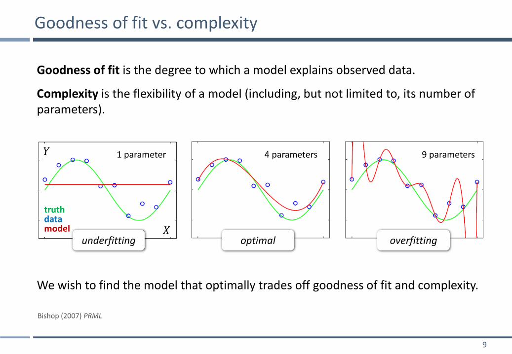
Goodness of fit vs. complexity

Goodness of fit is the degree to which a model explains observed data.

Complexity is the flexibility of a model (including, but not limited to, its number of parameters).

4 parameters 9 parameters

Bishop (2007) PRML

1 parameter

𝑋

𝑌

We wish to find the model that optimally trades off goodness of fit and complexity.

underfitting overfitting optimal

truth data model

10

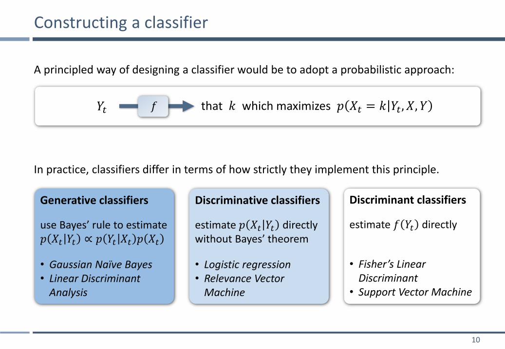
A principled way of designing a classifier would be to adopt a probabilistic approach:

Constructing a classifier

Generative classifiers

use Bayes’ rule to estimate 𝑝 𝑋𝑡 𝑌𝑡 ∝ 𝑝 𝑌𝑡 𝑋𝑡 𝑝 𝑋𝑡

• Gaussian Naïve Bayes • Linear Discriminant

Analysis

Discriminative classifiers

estimate 𝑝 𝑋𝑡 𝑌𝑡 directly without Bayes’ theorem

• Logistic regression • Relevance Vector

Machine

Discriminant classifiers

estimate 𝑓 𝑌𝑡 directly

• Fisher’s Linear Discriminant

• Support Vector Machine

𝑓 𝑌𝑡 that 𝑘 which maximizes 𝑝 𝑋𝑡 = 𝑘 𝑌𝑡, 𝑋, 𝑌

In practice, classifiers differ in terms of how strictly they implement this principle.

11

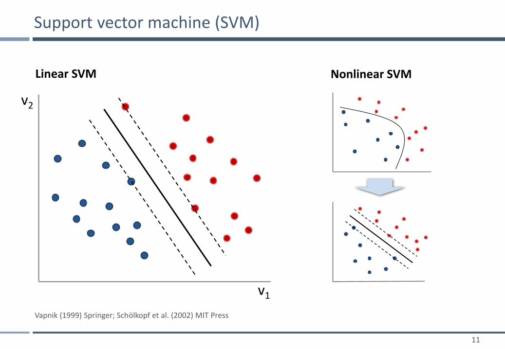
Support vector machine (SVM)

Vapnik (1999) Springer; Schölkopf et al. (2002) MIT Press

Nonlinear SVM Linear SVM

v1

v2

12

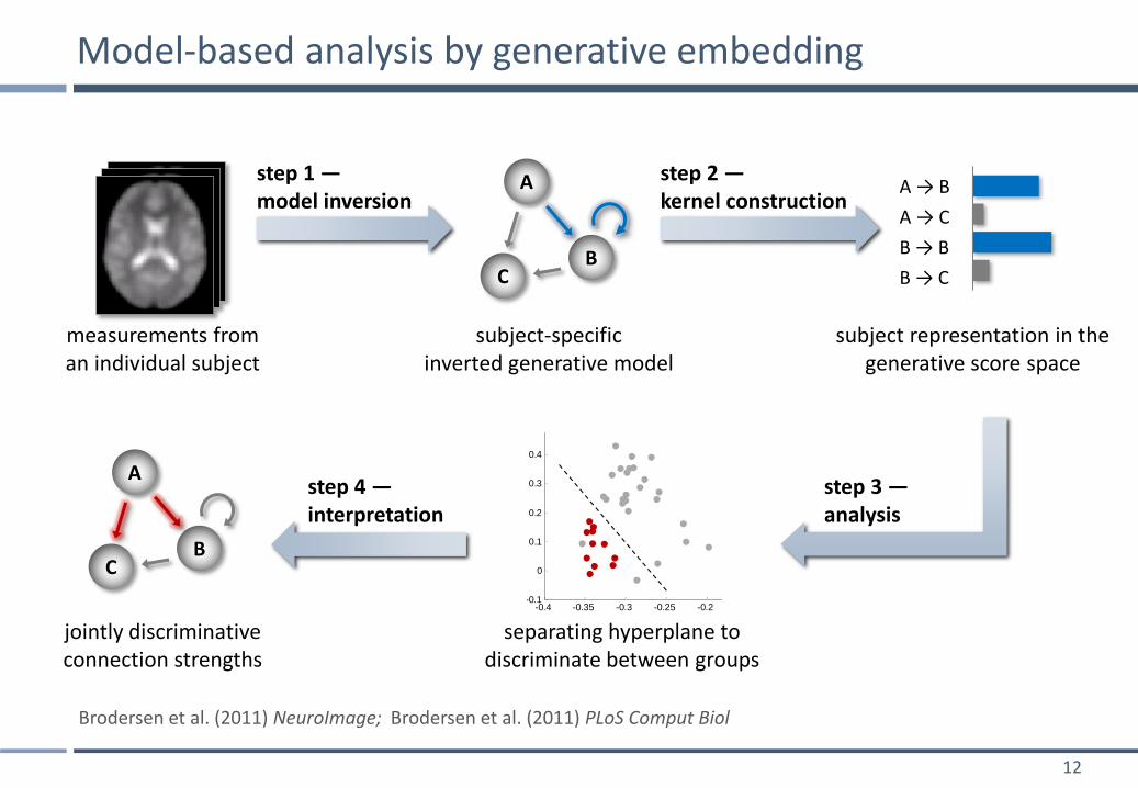
Model-based analysis by generative embedding

step 2 — kernel construction

step 1 — model inversion

measurements from an individual subject

subject-specific inverted generative model

subject representation in the generative score space

A → B

A → C

B → B

B → C

A

C B

step 3 — analysis

separating hyperplane to discriminate between groups

A

C B

jointly discriminative connection strengths

step 4 — interpretation

-2 0 2 4 6 8-1

0

1

2

3

4

5

Voxel 1

Voxe

l 2

-0.4 -0.35 -0.3 -0.25 -0.2 -0.15-0.1

0

0.1

0.2

0.3

0.4

0.5

0.6

(1) L.MGB -> L.MGB

(14)

R.H

G -

> L

.HG

Brodersen et al. (2011) NeuroImage; Brodersen et al. (2011) PLoS Comput Biol

13

activity 𝑧1(𝑡)

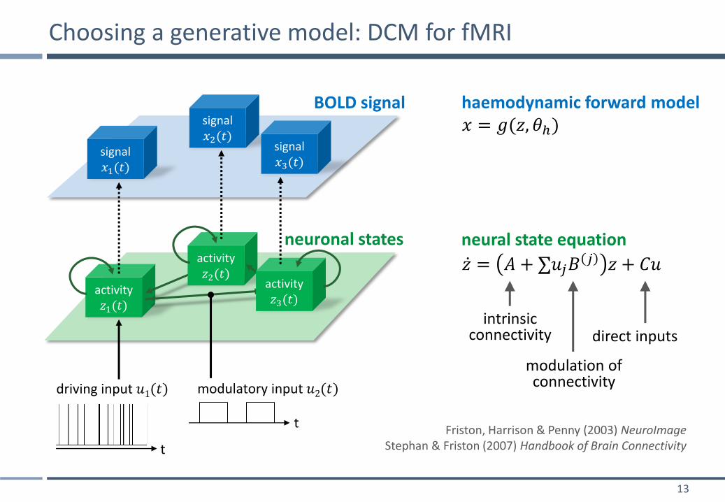
Choosing a generative model: DCM for fMRI

intrinsic connectivity direct inputs

modulation of connectivity

neural state equation

haemodynamic forward model 𝑥 = 𝑔(𝑧, 𝜃ℎ)

BOLD signal

neuronal states

t

driving input 𝑢1(𝑡) modulatory input 𝑢2(𝑡)

t

activity 𝑧2(𝑡)

activity 𝑧3(𝑡)

signal 𝑥1(𝑡)

signal 𝑥2(𝑡)

signal 𝑥3(𝑡)

Friston, Harrison & Penny (2003) NeuroImage Stephan & Friston (2007) Handbook of Brain Connectivity

𝑧 = 𝐴 + ∑𝑢𝑗𝐵𝑗 𝑧 + 𝐶𝑢

14

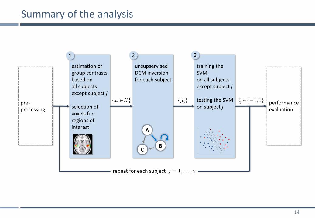
Summary of the analysis

pre-processing

estimation of group contrasts based on all subjects except subject j selection of voxels for regions of interest

unsupservised DCM inversion for each subject

training the SVM on all subjects except subject j testing the SVM on subject j

performance evaluation

1 2 3

repeat for each subject

A

C B

15

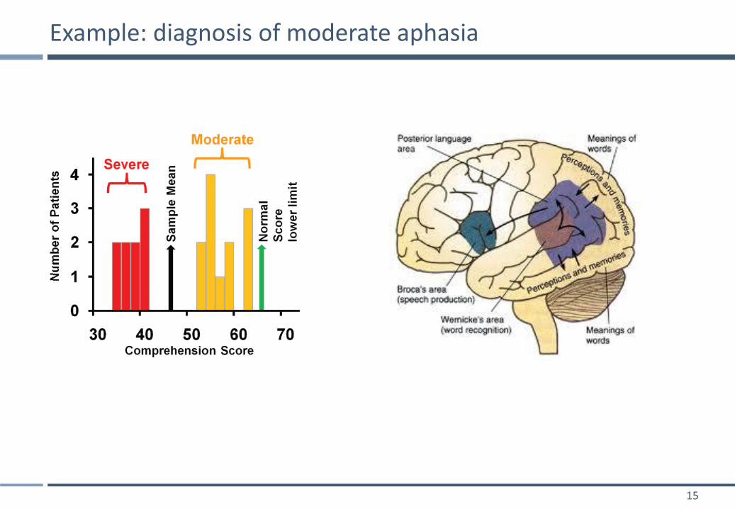
Example: diagnosis of moderate aphasia

16

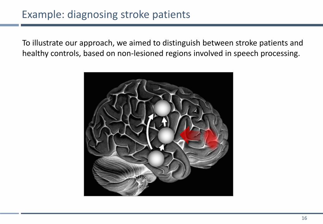
Example: diagnosing stroke patients

To illustrate our approach, we aimed to distinguish between stroke patients and healthy controls, based on non-lesioned regions involved in speech processing.

17

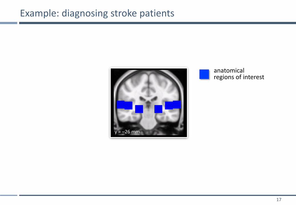
Example: diagnosing stroke patients

anatomical regions of interest

y = –26 mm

18

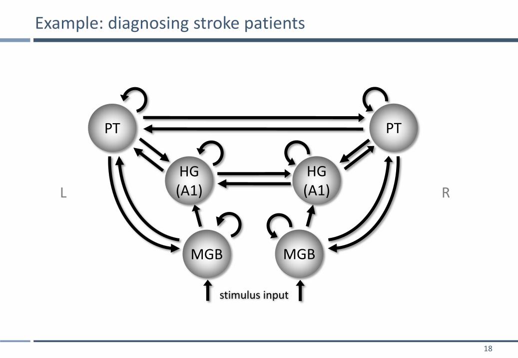
Example: diagnosing stroke patients

MGB

PT

HG (A1)

MGB

PT

HG (A1)

stimulus input

L R

19

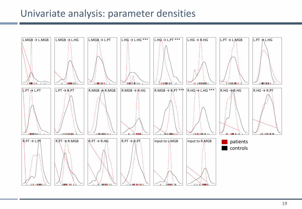
Univariate analysis: parameter densities

range(d1$x, d2$x) range(d1$x, d2$x) range(d1$x, d2$x) range(d1$x, d2$x) range(d1$x, d2$x) range(d1$x, d2$x) range(d1$x, d2$x) range(d1$x, d2$x)

range(d1$x, d2$x) range(d1$x, d2$x) range(d1$x, d2$x) range(d1$x, d2$x) range(d1$x, d2$x) range(d1$x, d2$x) range(d1$x, d2$x) range(d1$x, d2$x)

L.MGB → L.MGB L.MGB → L.HG L.MGB → L.PT L.HG → L.HG *** L.HG → L.PT *** L.HG → R.HG L.PT → L.MGB L.PT → L.HG

L.PT → L.PT L.PT → R.PT R.MGB → R.MGB R.MGB → R.HG R.MGB → R.PT *** R.HG → L.HG *** R.HG → R.HG R.HG → R.PT

R.PT → L.PT R.PT → R.MGB R.PT → R.HG R.PT → R.PT input to L.MGB input to R.MGB patients controls

20

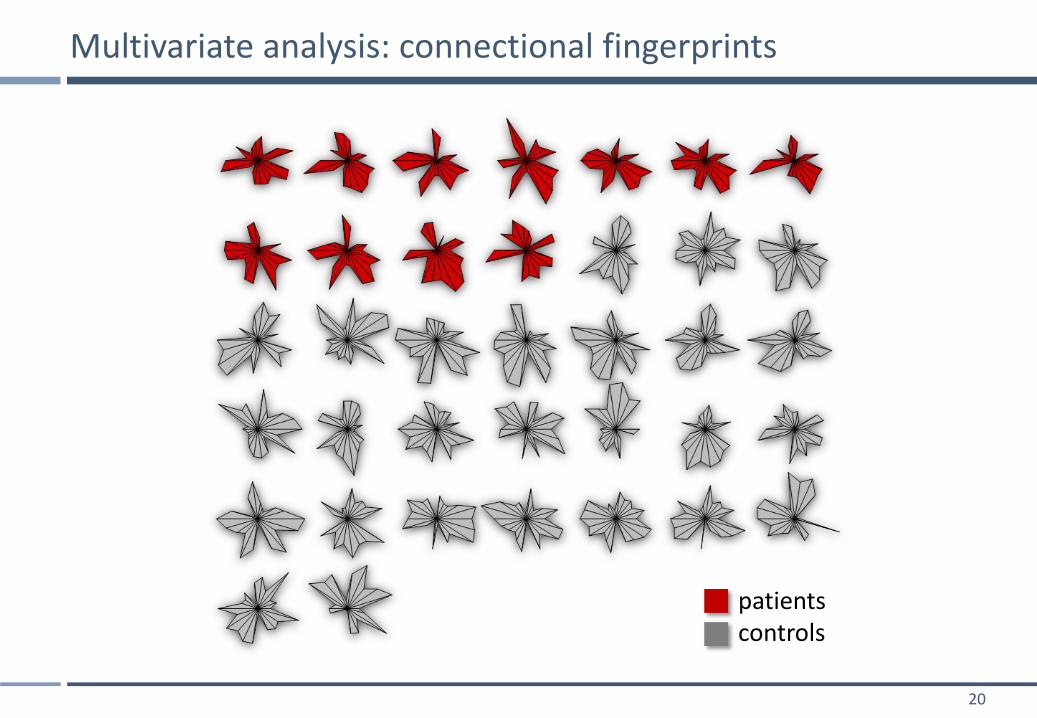
Multivariate analysis: connectional fingerprints

patients controls

21

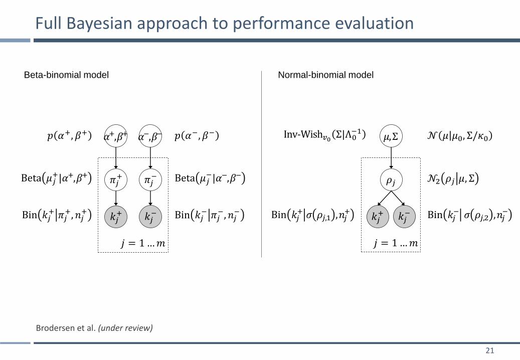
Full Bayesian approach to performance evaluation

Brodersen et al. (under review)

Beta-binomial model

𝑘𝑗+ 𝑘𝑗

−

𝜋𝑗+ 𝜋𝑗

−

𝛼+,𝛽+ 𝛼−,𝛽−

𝑘𝑗+ 𝑘𝑗

−

𝜌𝑗

𝜇,Σ

𝑗 = 1…𝑚

Bin 𝑘𝑗− 𝜎 𝜌𝑗,2 ,𝑛𝑗

− Bin 𝑘𝑗

+ 𝜎 𝜌𝑗,1 ,𝑛𝑗+

𝒩2 𝜌𝑗 𝜇, Σ

𝒩 𝜇 𝜇0, Σ/𝜅0

Bin 𝑘𝑗+ 𝜋𝑗

+, 𝑛𝑗+

Bin 𝑘𝑗− 𝜋𝑗

−, 𝑛𝑗−

Beta 𝜇𝑗−|𝛼−,𝛽− Beta 𝜇𝑗

+|𝛼+,𝛽+

𝑝 𝛼−, 𝛽− 𝑝 𝛼+, 𝛽+

𝑗 = 1…𝑚

Inv-Wish𝑣0 Σ|Λ0−1

Normal-binomial model

22

16218917734729133230781 24338936050

60

70

80

90

100

bala

nced

accu

racy

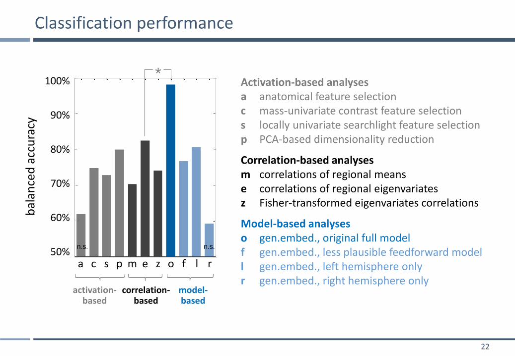
Classification performance

Activation-based analyses a anatomical feature selection c mass-univariate contrast feature selection s locally univariate searchlight feature selection p PCA-based dimensionality reduction

Correlation-based analyses m correlations of regional means e correlations of regional eigenvariates z Fisher-transformed eigenvariates correlations

Model-based analyses o gen.embed., original full model f gen.embed., less plausible feedforward model l gen.embed., left hemisphere only r gen.embed., right hemisphere only

activation- based

correlation- based

model- based

a c s p m e z o f l r

bal

ance

d a

ccu

racy

100%

50%

90%

80%

70%

60%

n.s. n.s.

*

23

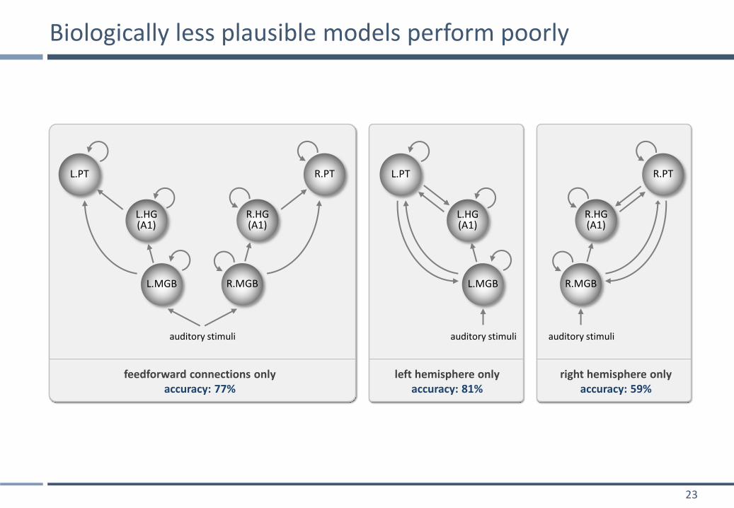
Biologically less plausible models perform poorly

L.MGB

L.PT

L.HG (A1)

R.MGB

R.PT

R.HG (A1)

L.MGB

L.PT

L.HG (A1)

R.MGB

R.PT

R.HG (A1)

auditory stimuli auditory stimuli auditory stimuli

feedforward connections only accuracy: 77%

left hemisphere only accuracy: 81%

right hemisphere only accuracy: 59%

24

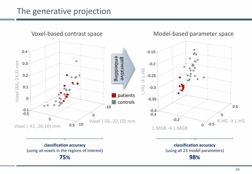
The generative projection

-10

0

10

-0.5

0

0.5

-0.1

0

0.1

0.2

0.3

0.4

-0.4

-0.2

0 -0.5

0

0.5-0.4

-0.35

-0.3

-0.25

-0.2

-0.15

-10

0

10

-0.5

0

0.5

-0.1

0

0.1

0.2

0.3

0.4

-0.4

-0.2

0 -0.5

0

0.5-0.4

-0.35

-0.3

-0.25

-0.2

-0.15

generative

emb

ed

din

g

L.H

G →

L.H

G

Vo

xel (

64

,-2

4,4

) m

m

L.MGB → L.MGB Voxel (-42,-26,10) mm Voxel (-56,-20,10) mm R.HG → L.HG

controls

patients

Voxel-based contrast space Model-based parameter space

classification accuracy (using all 23 model parameters)

98%

classification accuracy (using all voxels in the regions of interest)

75%

25

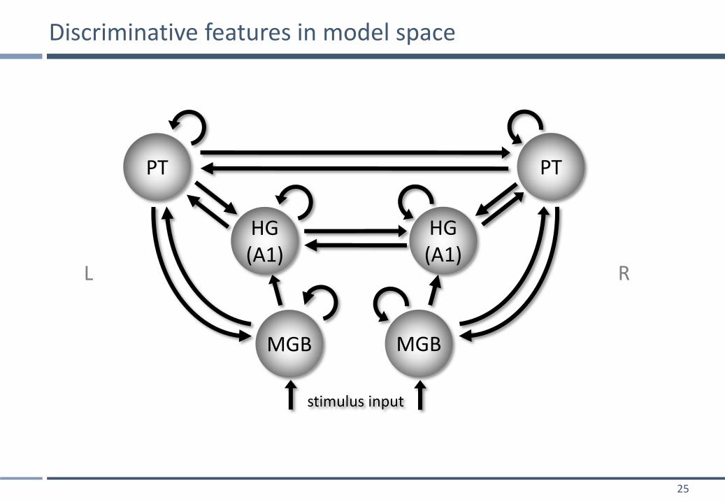
Discriminative features in model space

MGB

PT

HG (A1)

MGB

PT

HG (A1)

stimulus input

L R

26

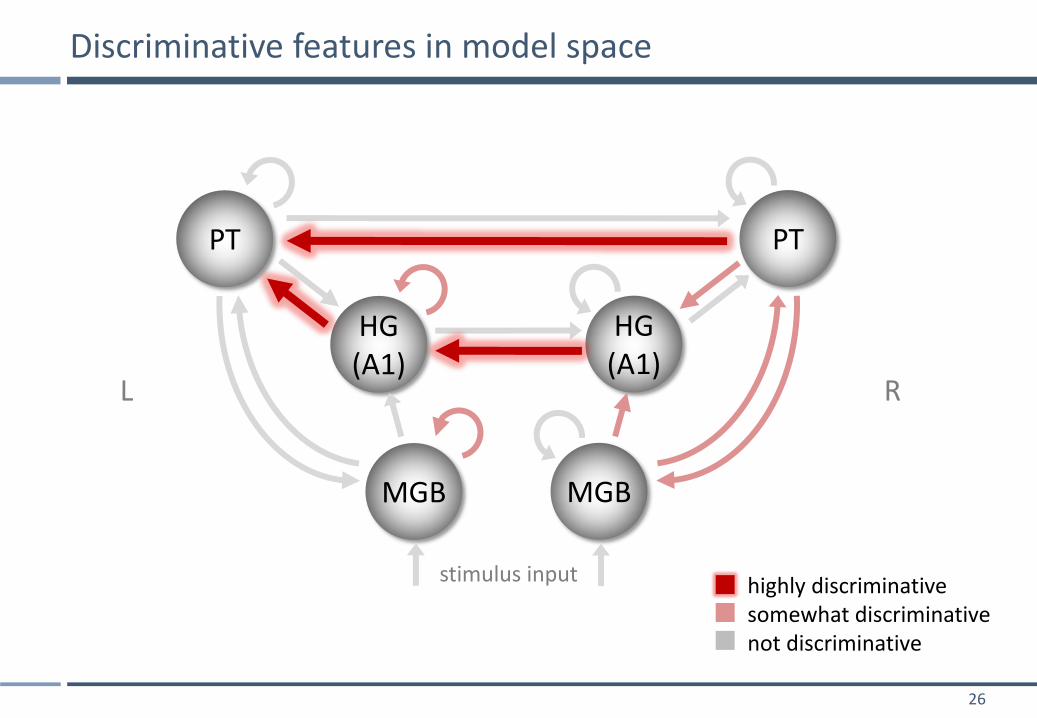
Discriminative features in model space

MGB

PT

HG (A1)

MGB

PT

HG (A1)

stimulus input

L R

highly discriminative somewhat discriminative not discriminative

27

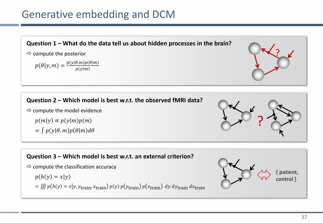
Question 1 – What do the data tell us about hidden processes in the brain?

compute the posterior

𝑝 𝜃 𝑦,𝑚 =𝑝 𝑦 𝜃,𝑚 𝑝 𝜃 𝑚

𝑝 𝑦 𝑚

Generative embedding and DCM

?

?

Question 2 – Which model is best w.r.t. the observed fMRI data?

compute the model evidence

𝑝 𝑚 𝑦 ∝ 𝑝 𝑦 𝑚 𝑝(𝑚)

= ∫ 𝑝 𝑦 𝜃,𝑚 𝑝 𝜃 𝑚 𝑑𝜃

Question 3 – Which model is best w.r.t. an external criterion?

compute the classification accuracy

𝑝 ℎ 𝑦 = 𝑥 𝑦

= 𝑝 ℎ 𝑦 = 𝑥 𝑦, 𝑦train, 𝑥train 𝑝 𝑦 𝑝 𝑦train 𝑝 𝑥train 𝑑𝑦 𝑑𝑦train 𝑑𝑥train

{ patient, control }

28

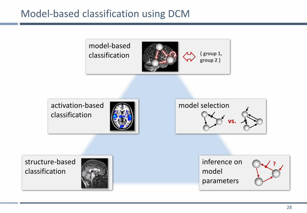
Model-based classification using DCM

structure-based classification

activation-based classification

model-based classification

model selection

inference on model parameters

vs.

?

{ group 1, group 2 }

29

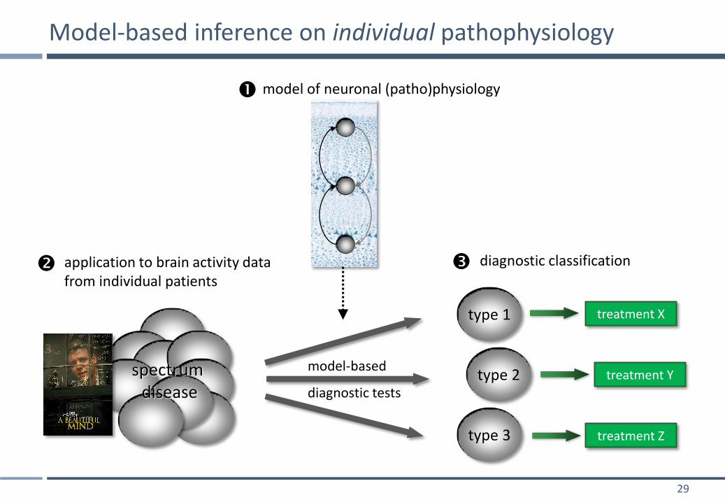
Model-based inference on individual pathophysiology

model-based

diagnostic tests

application to brain activity data from individual patients

model of neuronal (patho)physiology

spectrum disease

type 2

type 3

type 1

diagnostic classification

treatment X

treatment Y

treatment Z