Embed Size (px)
Citation preview

Model Assessment and Selection
Chapter 7
Neil Weisenfeld, et al.
Introduction
Generalization performance of a learning method:– Measure of prediction capability on
independent test data– Guide model selection– Give quantitative assessment of chosen
model
Chapter shows key methods and how to apply them to model selection
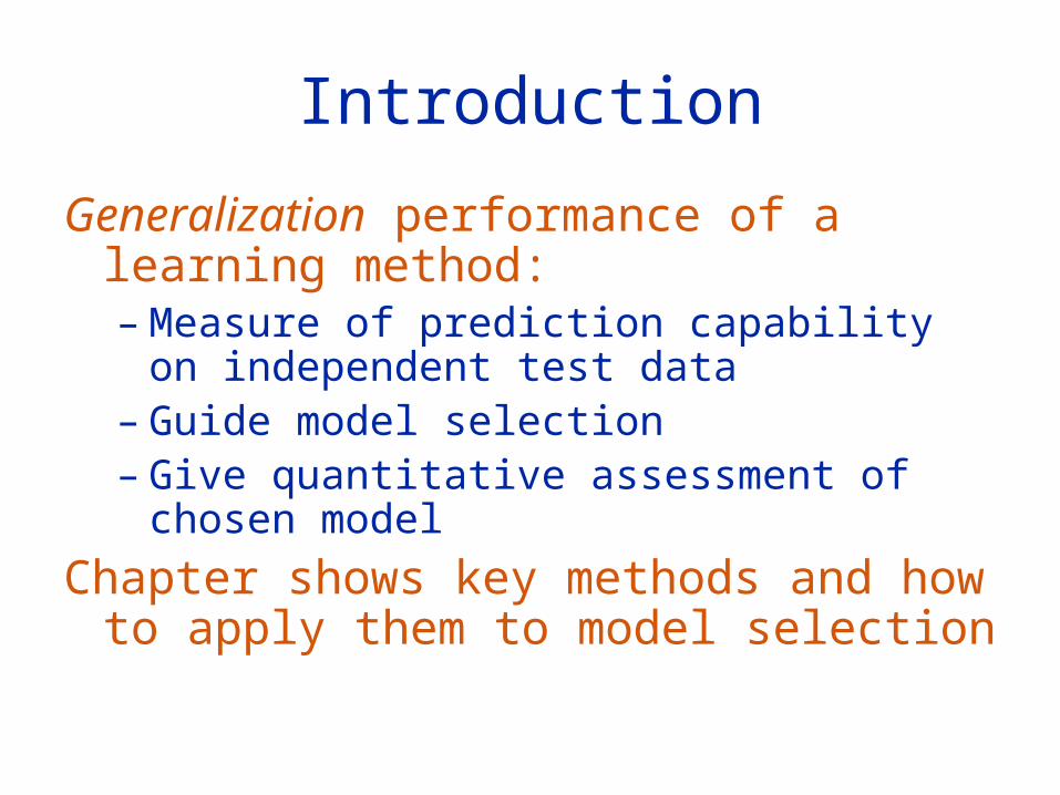
Bias, Variance, and Model Complexity
•Bias-Variance trade-off again•Generalization: test sample vs. training sample performance
– Training data usually monotonically increasing performance with model complexity
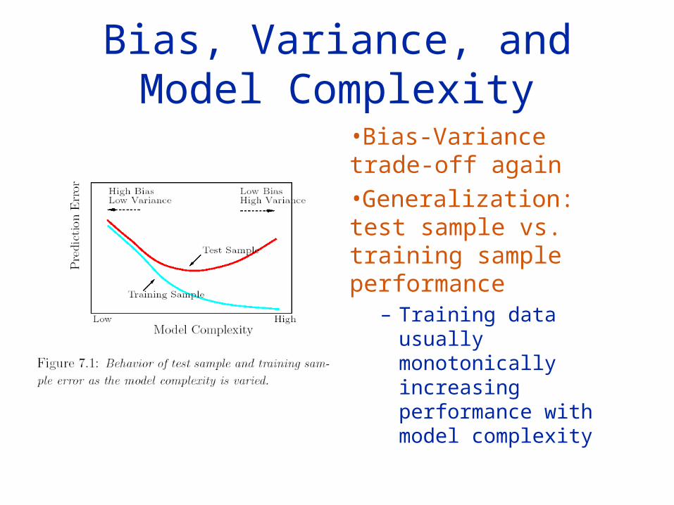
Measuring Performance
target variable
Vector of inputs
Prediction model
Typical Choices of Loss function
2ˆˆ,
ˆ
Y f X squared errorL Y f X
Y f X absolute error
YX
f X
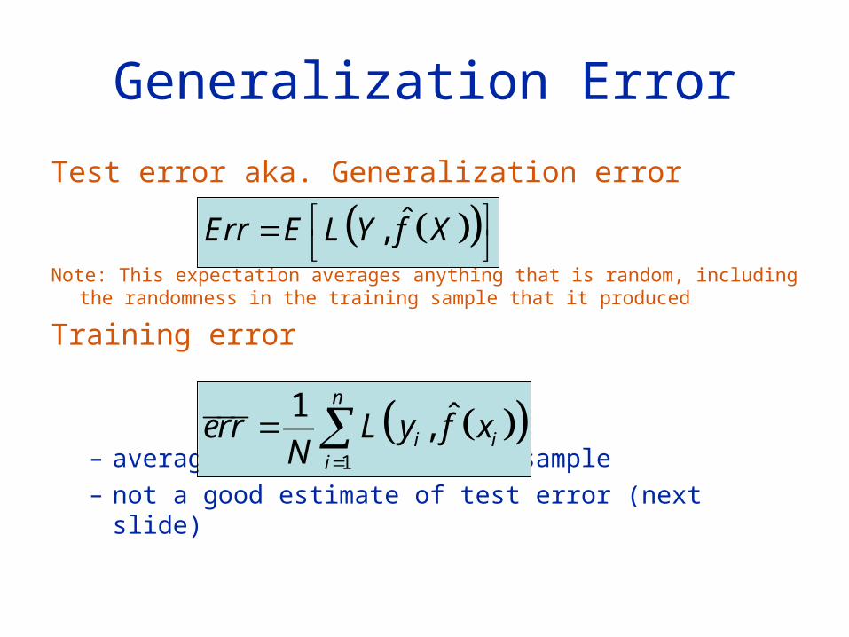
Test error aka. Generalization error
Note: This expectation averages anything that is random, including the randomness in the training sample that it produced
Training error
– average loss over training sample– not a good estimate of test error (next slide)
ˆ,Err E L Y f X
1
1 ˆ,n
i ii
err L y f xN
Generalization Error
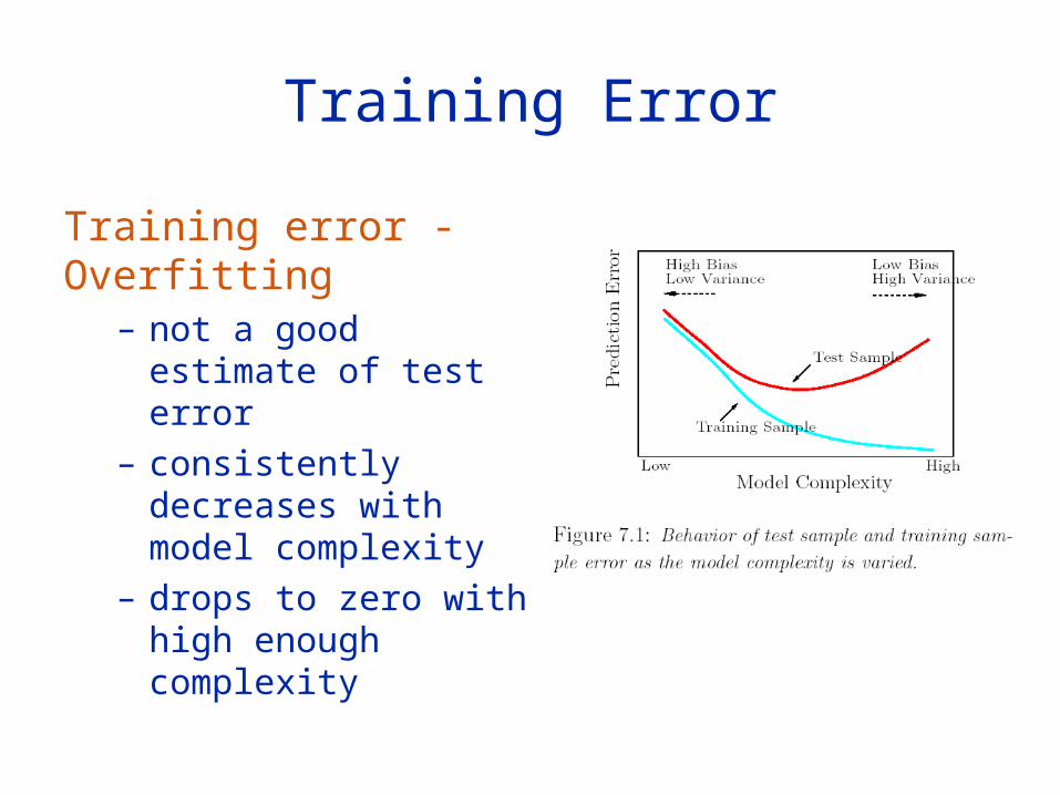
Training Error
Training error - Overfitting– not a good estimate of
test error– consistently decreases
with model complexity– drops to zero with high
enough complexity
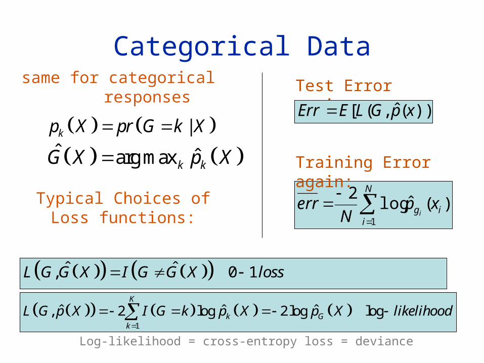
Categorical Datasame for categorical
responses
Typical Choices of Loss functions:
|kp X pr G k X
ˆ ˆarg maxk kG X p X
ˆ ˆ, 0 1 L G G X I G G X loss
1
ˆ ˆ ˆ, 2 log 2log logK
k Gk
L G p X I G k p X p X likelihood
Log-likelihood = cross-entropy loss = deviance
)(ˆlog2
1i
N
ig xp
Nerr
i
Training Error again:
Test Error again:
))](ˆ,([ xpGLEErr
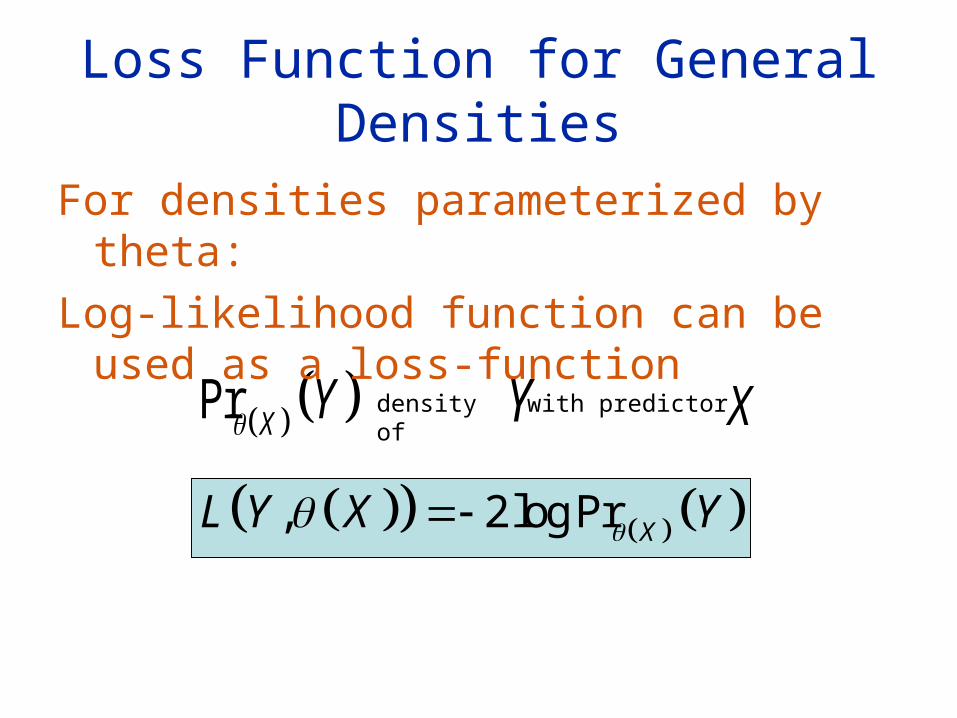
with predictor Pr X Y Ydensity of X
Loss Function for General Densities
For densities parameterized by theta:
Log-likelihood function can be used as a loss-function
, 2 log Pr XL Y X Y
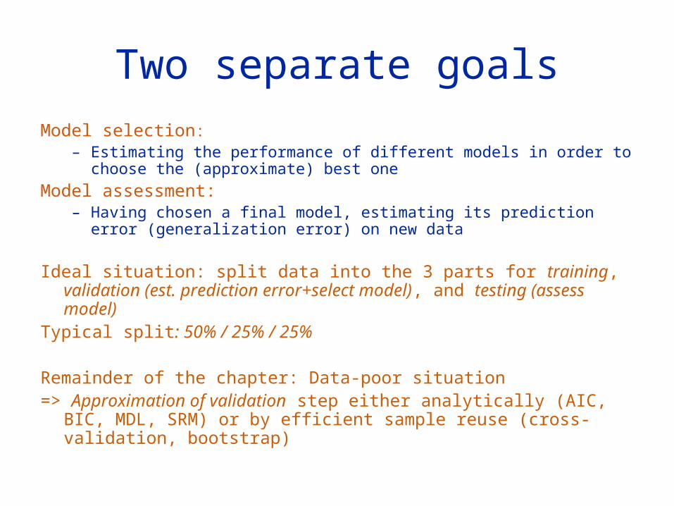
Two separate goals
Model selection:– Estimating the performance of different models in order to choose the
(approximate) best one
Model assessment:– Having chosen a final model, estimating its prediction error
(generalization error) on new data
Ideal situation: split data into the 3 parts for training, validation (est. prediction error+select model), and testing (assess model)
Typical split: 50% / 25% / 25%
Remainder of the chapter: Data-poor situation=> Approximation of validation step either analytically (AIC, BIC, MDL,
SRM) or by efficient sample reuse (cross-validation, bootstrap)
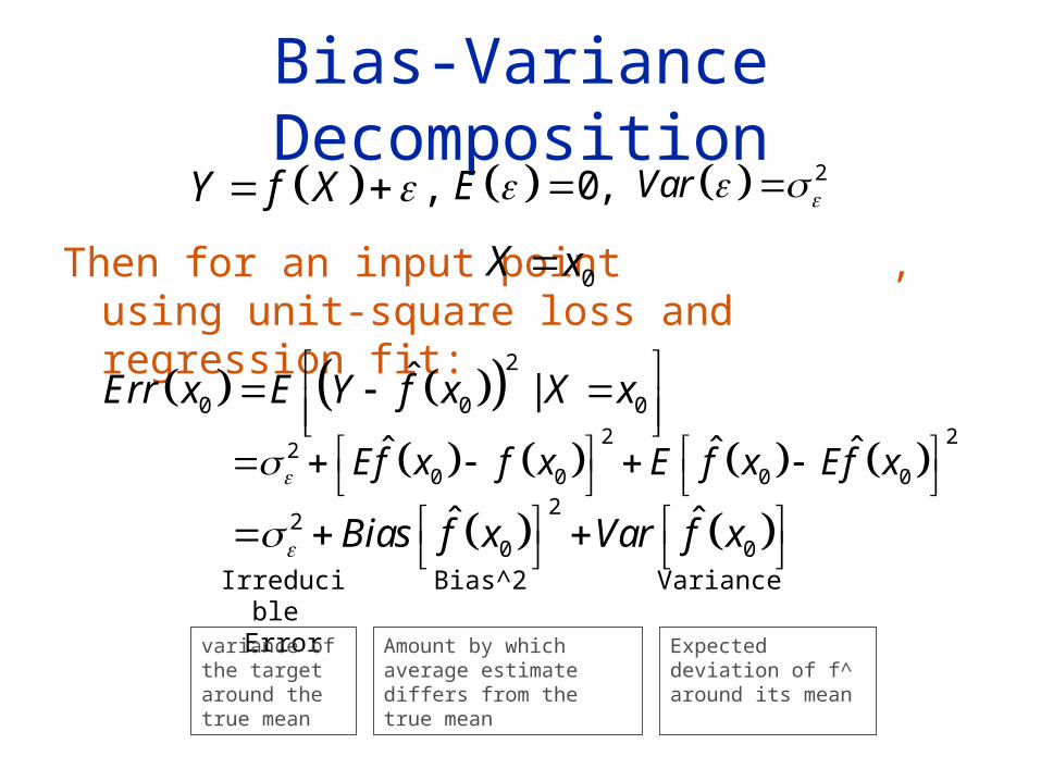
Bias-Variance Decomposition
Then for an input point , using unit-square loss and regression fit:
,Y f X 0,E 2Var
0X x
2
0 0 0ˆ |Err x E Y f x X x
2 22
0 0 0 0ˆ ˆ ˆEf x f x E f x Ef x
2
20 0
ˆ ˆBias f x Var f x Irreducible
ErrorBias^2 Variance
variance of the target around the true mean
Amount by which average estimate differs from the true mean
Expected deviation of f^ around its mean
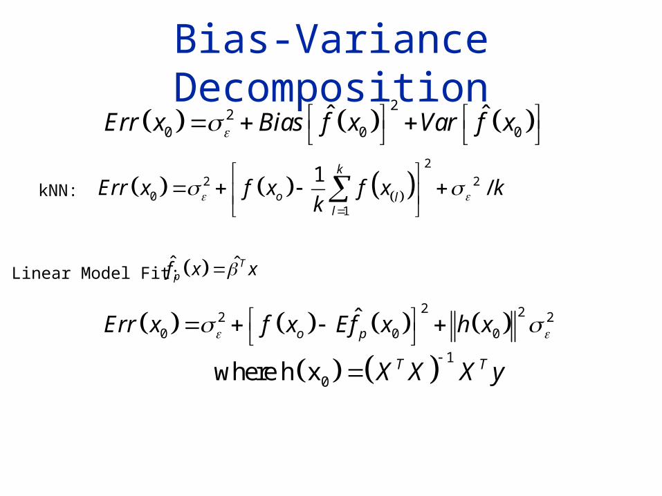
Bias-Variance Decomposition
22
0 0 0ˆ ˆErr x Bias f x Var f x
kNN: 2
2 20
1
1/
k
o ll
Err x f x f x kk
Linear Model Fit: ˆ ˆTpf x x
2 22 2
0 0 0ˆ
o pErr x f x Ef x h x
1
0where h x T TX X X y
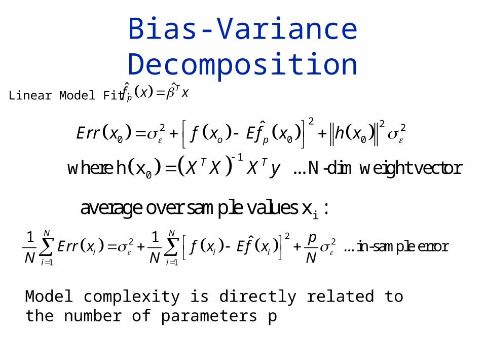
Bias-Variance Decomposition
Linear Model Fit: ˆ ˆTpf x x
2 22 2
0 0 0ˆ
o pErr x f x Ef x h x
1
0where h x ... N-dim weight vectorT TX X X y
iaverage over sample values x :
2
2 2
1 1
1 1 ˆ ... in-sample errorN N
i i ii i
pErr x f x Ef x
N N N
Model complexity is directly related to the number of parameters p
Bias-Variance Decomposition
22
0 0 0ˆ ˆErr x Bias f x Var f x
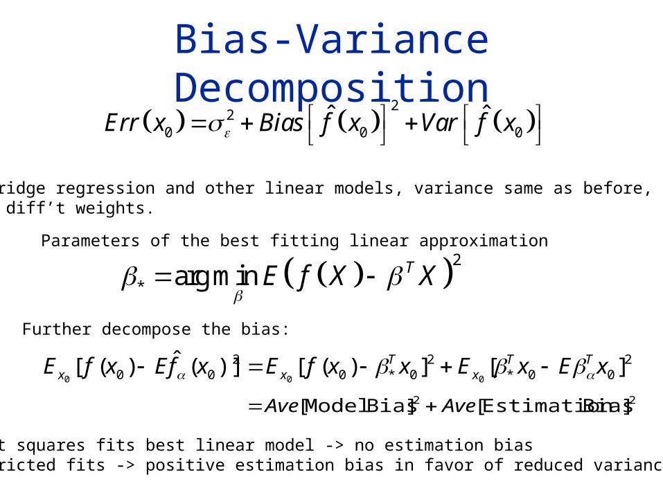
For ridge regression and other linear models, variance same as before, butwith diff’t weights.
2
* arg min TE f X X
Parameters of the best fitting linear approximation
Further decompose the bias:
200*
20*0
200 ][])([)](ˆ)([
000xExExxfExfExfE TT
xT
xx 22 ]Bias Estimation[]Bias Model[ AveAve
Least squares fits best linear model -> no estimation biasRestricted fits -> positive estimation bias in favor of reduced variance
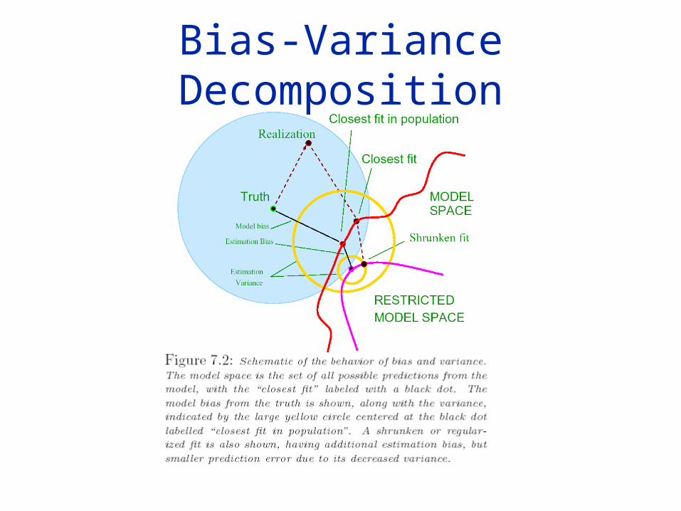
Bias-Variance Decomposition
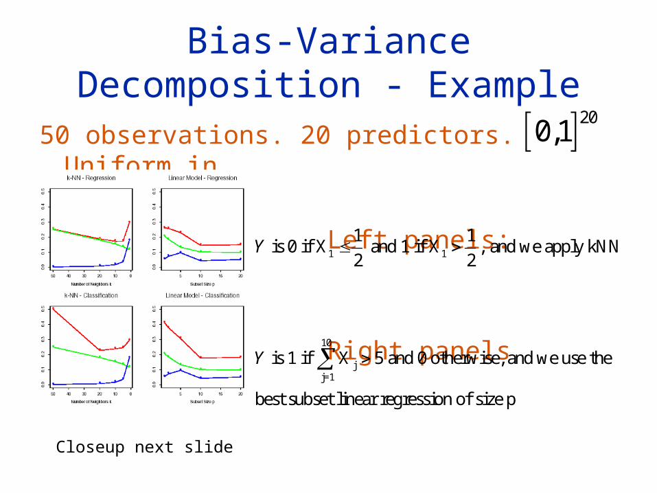
Bias-Variance Decomposition - Example
50 observations. 20 predictors. Uniform in
Left panels:
Right panels
200,1
1 1
1 1 is 0 if X and 1 if X , and we apply kNN
2 2Y
10
jj=1
is 1 if X 5 and 0 otherwise, and we use the
best subset linear regression of size p
Y
Closeup next slide
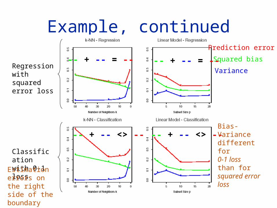
Example, continued
Regression with squared error loss
Classification with 0-1 loss
Prediction error
Squared bias
Variance
-- + -- = -- -- + -- = --
-- + -- <> -- -- + -- <> --Bias-Variance different for 0-1 loss than for squared error lossEstimation errors
on the right side of the boundary don’t hurt!
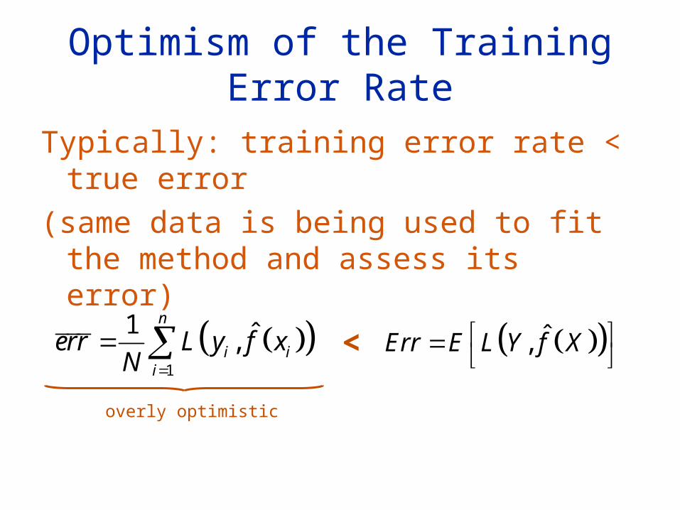
Optimism of the Training Error Rate
Typically: training error rate < true error
(same data is being used to fit the method and assess its error)
ˆ,Err E L Y f X 1
1 ˆ,n
i ii
err L y f xN
<
overly optimistic
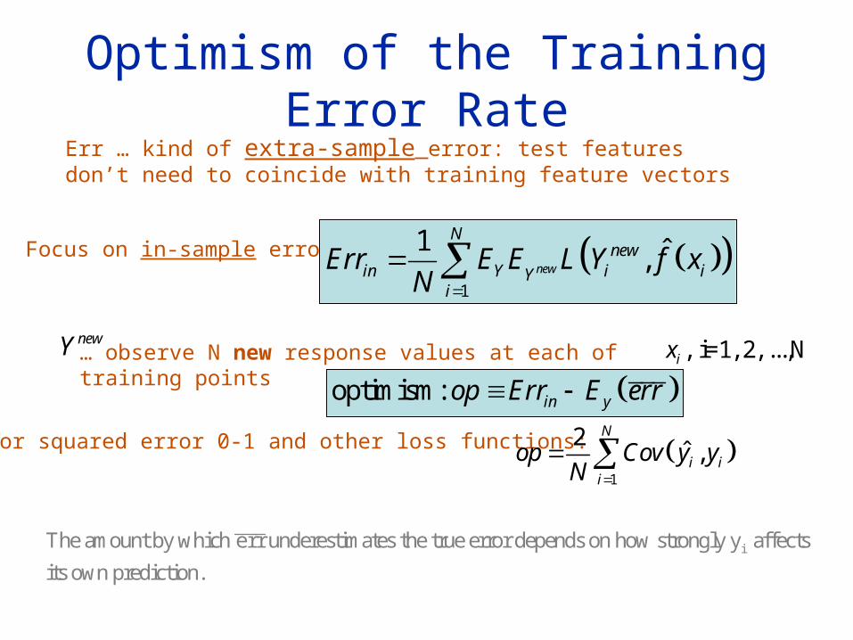
Optimism of the Training Error RateErr … kind of extra-sample error: test features don’t need to coincide with training feature vectors
Focus on in-sample error: 1
1 ˆ,new
Nnew
in Y i iYi
Err E E L Y f xN
newY … observe N new response values at each of training points , i=1, 2, ...,Nix
optimism: in yop Err E err
for squared error 0-1 and other loss functions: 1
2ˆ ,
N
i ii
op Cov y yN
iThe amount by which err underestimates the true error depends on how strongly y affects
its own prediction.
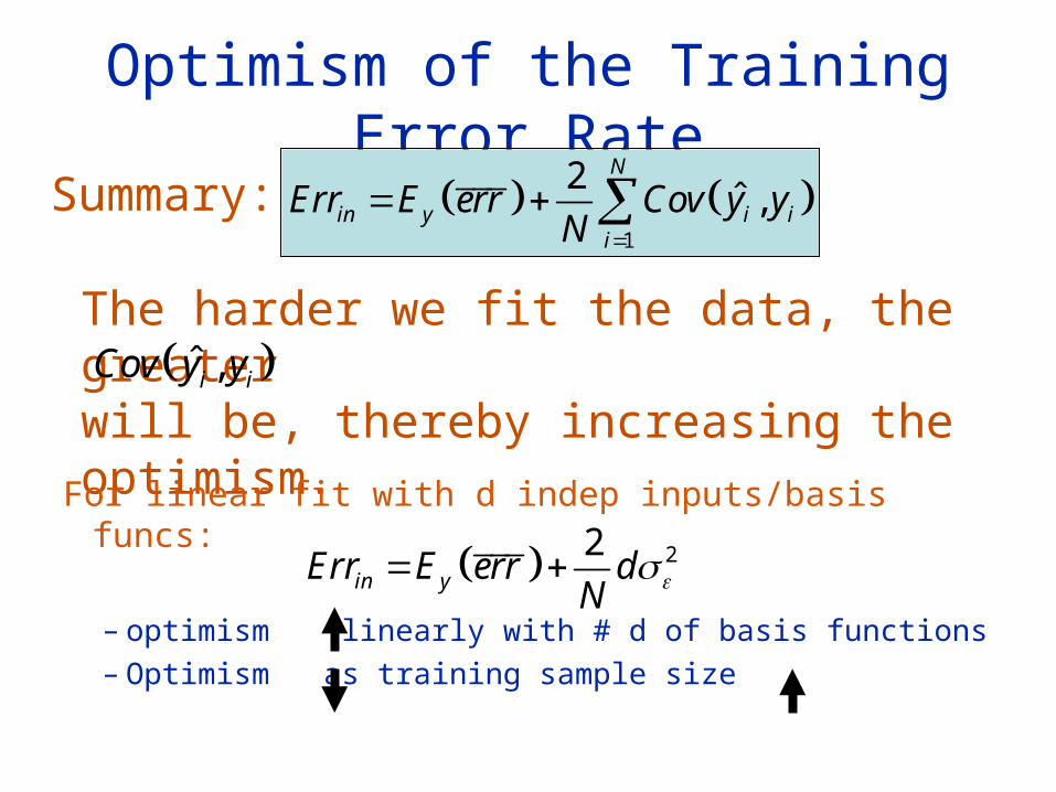
Optimism of the Training Error Rate
Summary: 1
2ˆ ,
N
in y i ii
Err E err Cov y yN
The harder we fit the data, the greater will be, thereby increasing the optimism.
ˆ ,i iCov y y
For linear fit with d indep inputs/basis funcs:
– optimism linearly with # d of basis functions– Optimism as training sample size
22in yErr E err d
N
Optimism of the Training Error Rate
Ways to estimate prediction error:– Estimate optimism and then add it to training error
rate • AIC, BIC, and others work this way, for a special class of
estimates that are linear in their parameters
– Direct estimates of the sample error • Cross-validation, bootstrap• Can be used with any loss function, and with nonlinear,
adaptive fitting techniques
err
Err
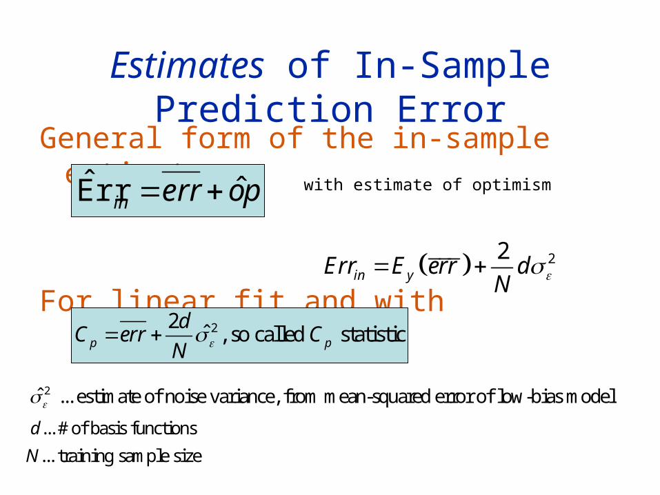
Estimates of In-Sample Prediction Error
General form of the in-sample estimate:
For linear fit and with : 22in yErr E err d
N
22ˆ , so called statisticp p
dC err C
N
2ˆ ... estimate of noise variance, from mean-squared error of low-bias model
... # of basis functionsd
... training sample sizeN
poerrin ˆrrE with estimate of optimism
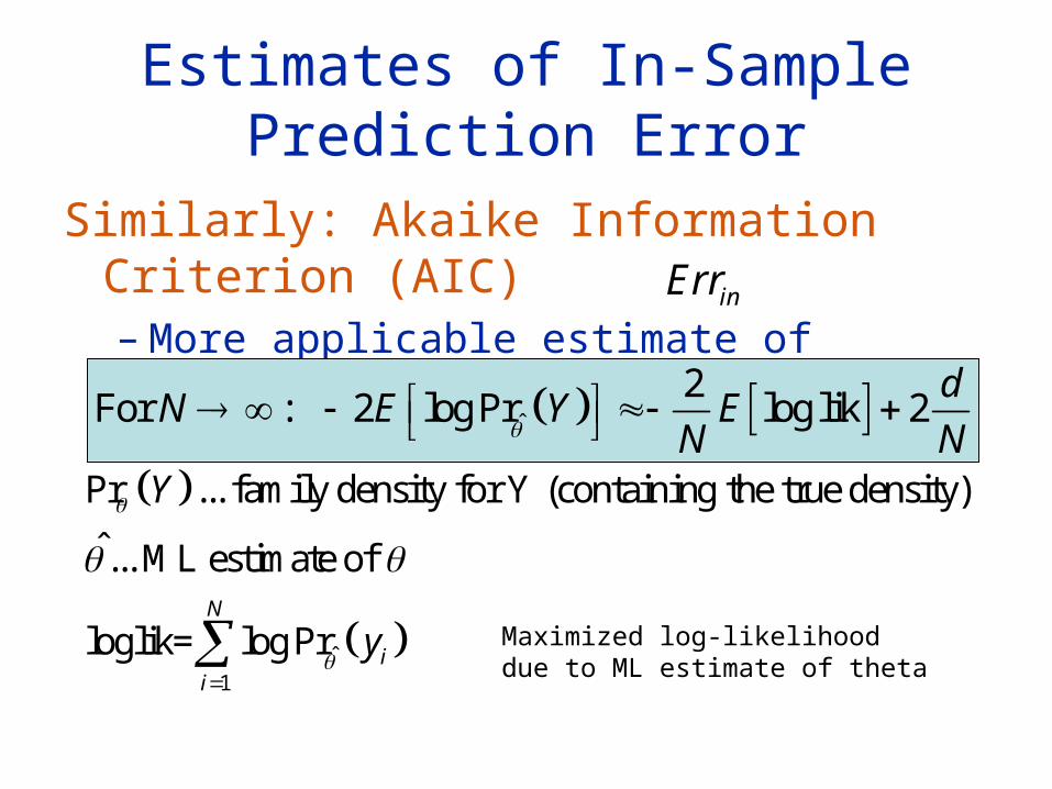
Estimates of In-Sample Prediction Error
Similarly: Akaike Information Criterion (AIC)– More applicable estimate of , when log-
likelihood function is usedinErr
ˆ
2For : 2 log Pr log lik 2
dN E Y E
N N
ˆ1
Pr ... family density for Y (containing the true density)
ˆ... ML estimate of
loglik= log PrN
ii
Y
y
Maximized log-likelihood due to ML
estimate of theta
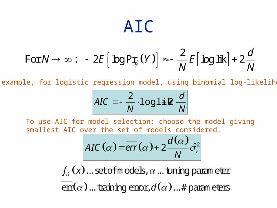
AIC
ˆ
2For : 2 log Pr log lik 2
dN E Y E
N N
For example, for logistic regression model, using binomial log-likelihood:
To use AIC for model selection: choose the model giving smallest AIC over the set of models considered.
2ˆ2d
AIC errN
ˆ ... set of models, ... tuning parameter
err ... training error, ... # parameters
f x
d
N
d
NAIC 2loglik
2
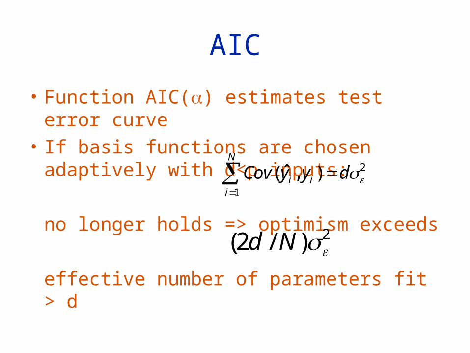
AIC
• Function AIC() estimates test error curve
• If basis functions are chosen adaptively with d<p inputs:
no longer holds => optimism exceeds
effective number of parameters fit > d
2
1
),ˆ( dyyCov i
N
ii
2)/2( Nd
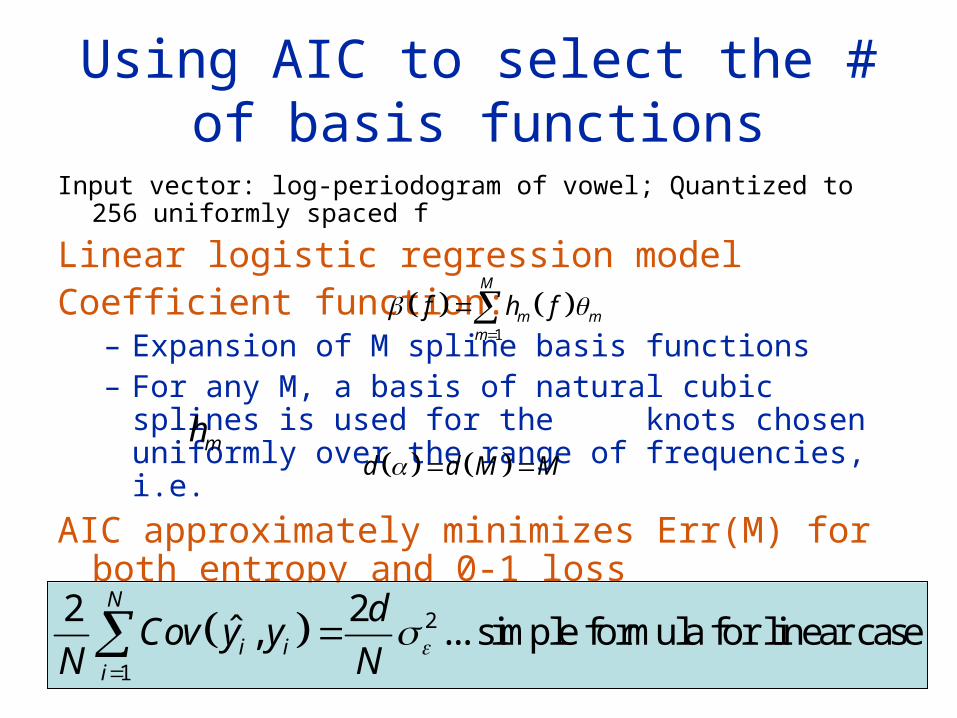
Using AIC to select the # of basis functions
Input vector: log-periodogram of vowel; Quantized to 256 uniformly spaced f
Linear logistic regression model Coefficient function:
– Expansion of M spline basis functions– For any M, a basis of natural cubic splines is used for
the knots chosen uniformly over the range of frequencies, i.e.
AIC approximately minimizes Err(M) for both entropy and 0-1 loss
1
M
m mm
f h f
mh d d M M
2
1
2 2ˆ , ... simple formula for linear case
N
i ii
dCov y y
N N
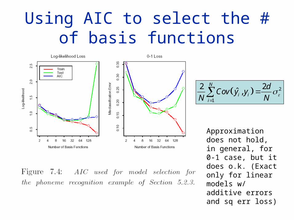
Using AIC to select the # of basis functions
2
1
2 2ˆ ,
N
i ii
dCov y y
N N
Approximation does not hold, in general, for 0-1 case, but it does o.k. (Exact only for linear models w/ additive errors and sq err loss)
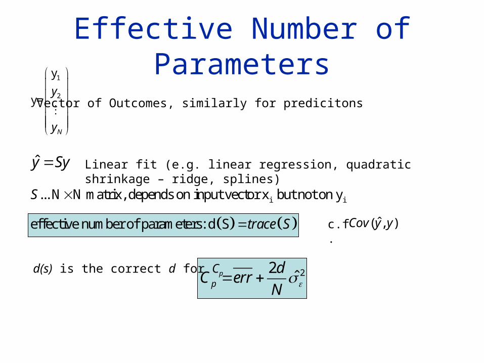
Effective Number of Parameters1
2
y
y=
N
y
y
Vector of Outcomes, similarly for predicitons
y Sy Linear fit (e.g. linear regression, quadratic shrinkage – ridge, splines)
i i... N N matrix, depends on input vector x but not on yS
effective number of parameters: d S trace S
22ˆp
dC err
N
c.f. ),ˆ( yyCov
d(s) is the correct d for Cp
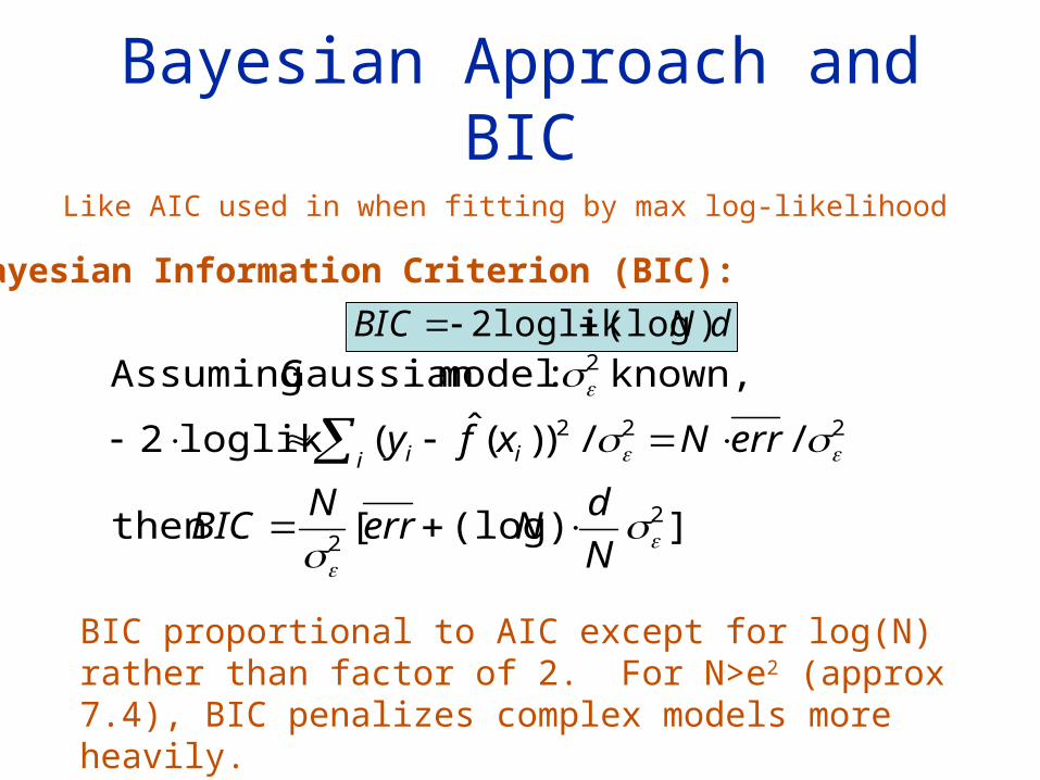
Bayesian Approach and BIC
Like AIC used in when fitting by max log-likelihood
BIC proportional to AIC except for log(N) rather than factor of 2. For N>e2 (approx 7.4), BIC penalizes complex models more heavily.
Bayesian Information Criterion (BIC):
])(log[then
//))(ˆ(loglik2
known, :modelGaussian Assuming
22
222
2
N
dNerr
NBIC
errNxfyi ii
dNCBI )(logloglik2
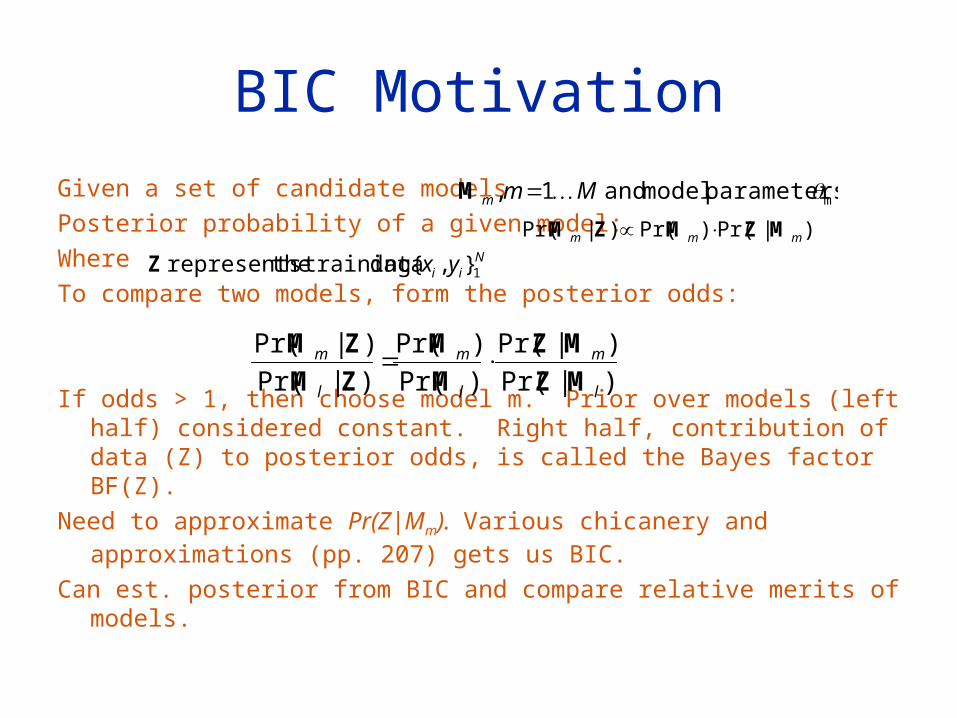
BIC Motivation
Given a set of candidate models
Posterior probability of a given model:
Where
To compare two models, form the posterior odds:
If odds > 1, then choose model m. Prior over models (left half) considered constant. Right half, contribution of data (Z) to posterior odds, is called the Bayes factor BF(Z).
Need to approximate Pr(Z|Mm). Various chicanery and approximations (pp. 207) gets us BIC.
Can est. posterior from BIC and compare relative merits of models.
m parameters model and 1, Mmm Μ
)|Pr()Pr()|Pr( mmm MZMZM N
ii yx 1},{ data training therepresents Z
)|Pr(
)|Pr(
)Pr(
)Pr(
)|Pr(
)|Pr(
l
m
l
m
l
m
MZ
MZ
M
M
ZM
ZM

BIC: How much better is a model?
But we may want to know how various models stack up (not just ranking) relative to one another:
Once we have the BIC:
Denominator normalizes the result and now we can assess the relative merits of each model
M
l
BIC
BIC
ml
m
e
e
12
1
2
1
)|Pr( of estimate ZM
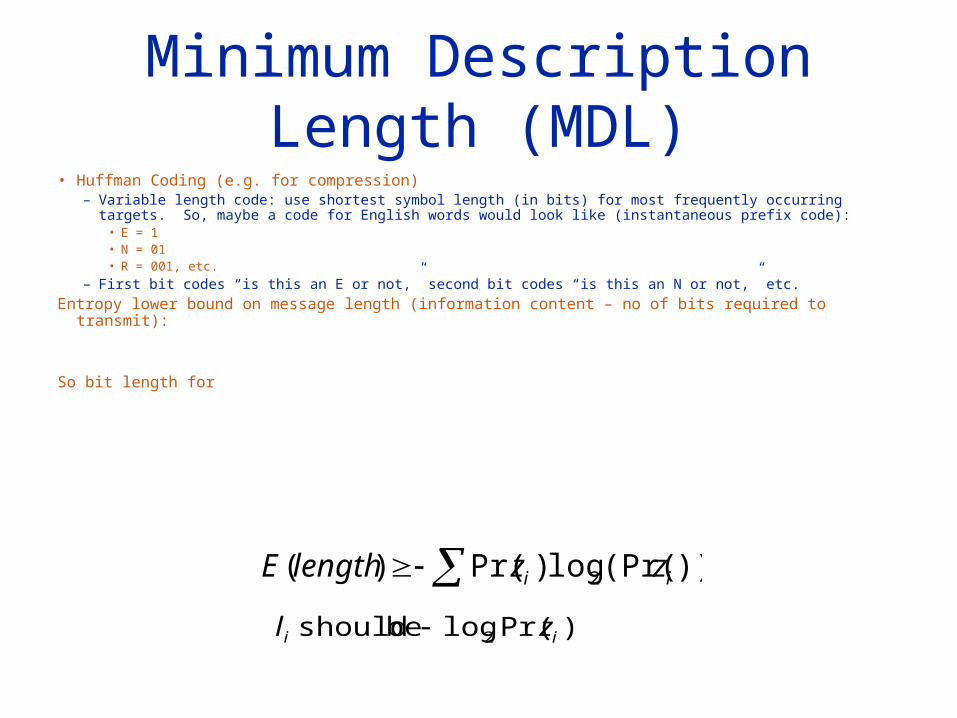
Minimum Description Length (MDL)
• Huffman Coding (e.g. for compression)– Variable length code: use shortest symbol length (in bits) for most frequently occurring targets. So, maybe a
code for English words would look like (instantaneous prefix code):• E = 1• N = 01• R = 001, etc.
– First bit codes “is this an E or not,” second bit codes “is this an N or not,” etc.
Entropy lower bound on message length (information content – no of bits required to transmit):
So bit length for
))(Pr(log)Pr()( 2 ii zzlengthE
)Pr(log be should 2 ii zl
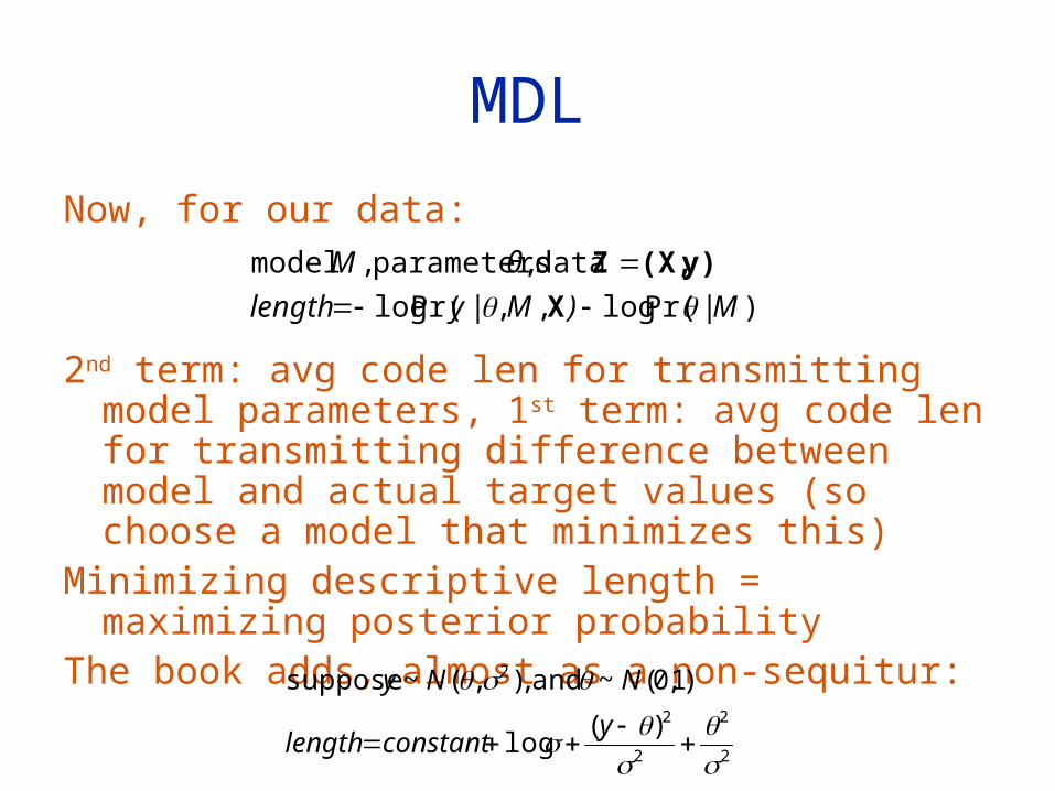
MDL
Now, for our data:
2nd term: avg code len for transmitting model parameters, 1st term: avg code len for transmitting difference between model and actual target values (so choose a model that minimizes this)
Minimizing descriptive length = maximizing posterior probability
The book adds, almost as a non-sequitur:
)|Pr(log,,|Pr(log
data , parameters , model
M)Mylength
θM
X
y)(X,Z
2
2
2
2
2
)(log
)1,0(~ and ,),(~ suppose
y
constantlength
NNy