Embed Size (px)
Citation preview
1 /14 | P a g e
MODEL ANSWER
AU-6423
Master of Business Administration (First Semester) Examination, 2014
Paper : Second
QUANTITATIVE METHODS
Time Allowed : Three Hours
Maximum Marks : 70
Minimum Pass Marks : 28
Note: Attempt both the sections as directed.
Note: Attempt all the questions. This section contains Ten short answer type questions having 2 Marks
each.
(10x2 = 20 Marks)
1. CONCURRENT DEVIATION METHOD
The method of studying correlation is the simplest of all the methods. The only thing that is
required under this method is to find out the direction of change of X variable and Y variable.
The formula applicable is:
rc = +√+ (2C-n)/n
Where rc stands for coefficient of correlation by the concurrent deviation method; C stands
for the number of concurrent deviations or the number of positive signs obtained after
multiplying
Dx with Dy; n = Number of pairs of observations compared.
Steps are as follows:
(i) Find out the direction of change of X variable, i.e., as compared with the first value,
whether the second value is increasing or decreasing or is constant. If it is increasing put (+)
sign; if it is decreasing put (-) sign (minus) and if it is constant put zero. Similarly, as
compared to second value find out whether the third value is increasing, decreasing or
constant. Repeat the same process for other values. Denote this column by Dx.
(ii) In the same manner as discussed above find out the direction of change of Y variable and
denote this column by Dy
(iii) Multiply Dx with Dy, and determine the value of c, i.e., the number of positive signs.
(iv) Apply the above formula, i.e.,
rc = +√+ (2C-n)/n
2. A graphical representation is a visual display of data and statistical results. It is often
more effective than presenting data in tabular form. There are many different types of
Section – A
2 /14 | P a g e
graphical representation and which is used depends on the nature of the data and the type
of statistical results.
a. Pie chart: An appropriate graphical representation of category frequencies is
a pie chart, where each slice represents a different category and slice angles are
proportional to the frequencies of the categories.
b. Bar chart: Another graphical method used for category frequencies is a bar chart,
where each bar represents a different category and the heights of the bars are
proportional to the frequencies of the categories.
c. Histogram and Frequency Polygram: For frequency distribution of continuous
quantitative data convenient graphs are a histogram, frequency polygon, and/or.
Some other common and suitable graphical representations are Stem-and-leaf plot,
Ogive Curve, Lorenz Curve, Line Chart etc.
3. A problem can be realistically represented as a linear program if the following
assumptions hold:
a. The constraints and objective function are linear.
b. This requires that the value of the objective function and the response of each
resource expressed by the constraints is proportional to the level of each
activity expressed in the variables.
c. Linearity also requires that the effects of the value of each variable on the
values of the objective function and the constraints are additive. In other
words, there can be no interactions between the effects of different activities;
i.e., the level of activity X1 should not affect the costs or benefits associated
with the level of activity X2.
d. Divisibility -- the values of decision variables can be fractions. Sometimes
these values only make sense if they are integers; then we need an extension of
linear programming called integer programming.
e. Certainty -- the model assumes that the responses to the values of the variables
are exactly equal to the responses represented by the coefficients.
f. Data -- formulating a linear program to solve a problem assumes that data are
available to specify the problem.
g. Non-negativity requirements as resources can’t hold negative values.
3 /14 | P a g e
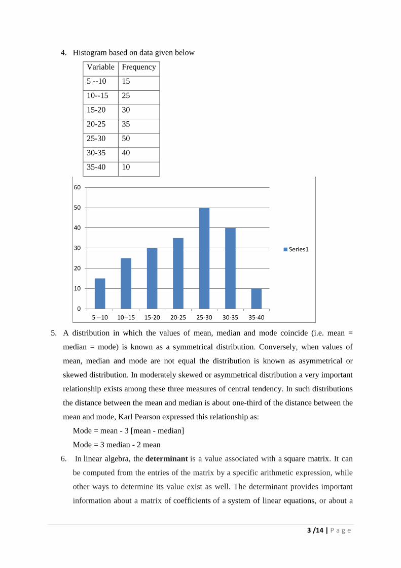
4. Histogram based on data given below
Variable Frequency
5 --10 15
10--15 25
15-20 30
20-25 35
25-30 50
30-35 40
35-40 10
5. A distribution in which the values of mean, median and mode coincide (i.e. mean =
median = mode) is known as a symmetrical distribution. Conversely, when values of
mean, median and mode are not equal the distribution is known as asymmetrical or
skewed distribution. In moderately skewed or asymmetrical distribution a very important
relationship exists among these three measures of central tendency. In such distributions
the distance between the mean and median is about one-third of the distance between the
mean and mode, Karl Pearson expressed this relationship as:
Mode = mean - 3 [mean - median]
Mode = 3 median - 2 mean
6. In linear algebra, the determinant is a value associated with a square matrix. It can
be computed from the entries of the matrix by a specific arithmetic expression, while
other ways to determine its value exist as well. The determinant provides important
information about a matrix of coefficients of a system of linear equations, or about a
0
10
20
30
40
50
60
5 --10 10--15 15-20 20-25 25-30 30-35 35-40
Series1
4 /14 | P a g e
matrix that corresponds to a linear transformation of a vector space. The determinant
of a matrix A is denoted det(A), det A, or |A|.[1]
In the case where the matrix entries are
written out in full, the determinant is denoted by surrounding the matrix entries by
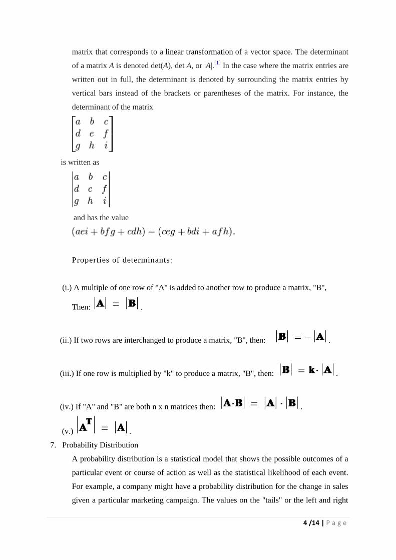
vertical bars instead of the brackets or parentheses of the matrix. For instance, the
determinant of the matrix
is written as
and has the value
Properties of determinants:
(i.) A multiple of one row of "A" is added to another row to produce a matrix, "B",
Then: .
(ii.) If two rows are interchanged to produce a matrix, "B", then: .
(iii.) If one row is multiplied by "k" to produce a matrix, "B", then: .
(iv.) If "A" and "B" are both n x n matrices then: .
(v.) .
7. Probability Distribution
A probability distribution is a statistical model that shows the possible outcomes of a
particular event or course of action as well as the statistical likelihood of each event.
For example, a company might have a probability distribution for the change in sales
given a particular marketing campaign. The values on the "tails" or the left and right
5 /14 | P a g e
end of the distribution are much less likely to occur than those in the middle of the
curve.
Importance of Probability distribution
a. Scenario Analysis: Probability distributions can be used to create scenario
analyses. A scenario analysis uses probability distributions to create several,
theoretically distinct possibilities for the outcome of a particular course of
action or future event. For example, a business might create three scenarios:
worst-case, likely and best-case.
b. Sales Forecasting: One practical use for probability distributions and scenario
analysis in business is to predict future levels of sales. It is essentially
impossible to predict the precise value of a future sales level; however,
businesses still need to be able to plan for future events.
c. Risk Evaluation: In addition to predicting future sales levels, probability
distribution can be a useful tool for evaluating risk.
d. Replacement Planning : Replacement of machines can be planned through
probability distribution
Similarly many other applications can be sighted by students.
8. To make decisions about everything from hiring to manufacturing volume, businesses
must engage in some level of forecasting. The area where most businesses employ
forecasting is sales. Forecasts, however, are made in a gray area that lacks certainty.
The absence of certainty stems from a number of factors that affect forecasts for
which the business cannot account or from problems with the available data.
Two important bases for forecasting are:
a. Historical data
b. Suitable mathematical model for forecasting
9. Periodic function is a function that repeats its values in regular intervals or periods.
The most important examples are the trigonometric functions, which repeat over
intervals of 2π radians. Periodic functions are used throughout science to
describe oscillations, waves, and other phenomena that exhibit periodicity. In business
administration product life cycle, business cycle are common example of periodic
functions.
10. 10. Number of ways taking 5 flags out of 8-flags = 8P5
= 8!/(8-5)!
= 8 x 7 x 6 x 5 x 4 = 6720
6 /14 | P a g e
Note: Attempt any five questions. This section contains Eight long- answer type questions carrying 10
marks each. (5x10=50 Marks).
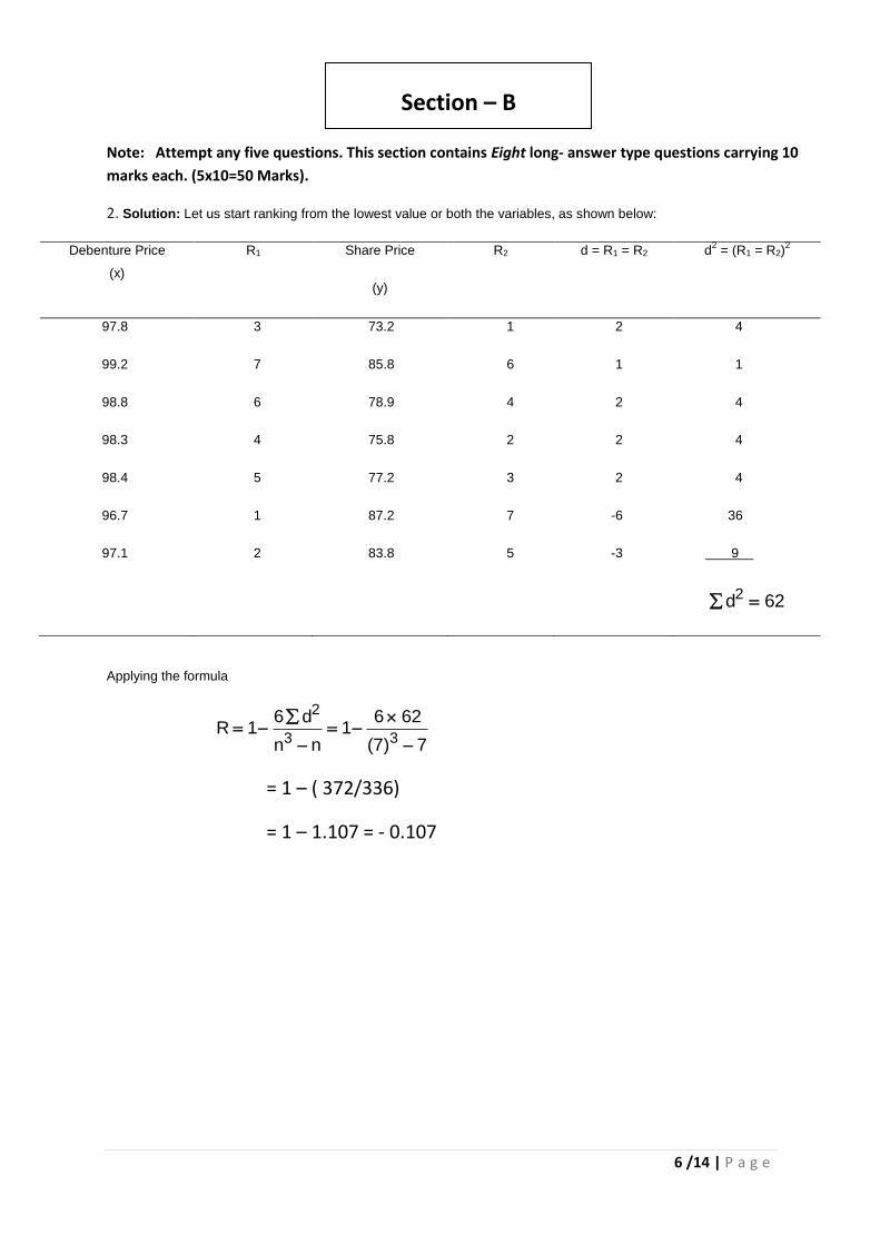
2. Solution: Let us start ranking from the lowest value or both the variables, as shown below:
Debenture Price
(x)
R1 Share Price
(y)
R2 d = R1 = R2 d2 = (R1 = R2)
2
97.8
99.2
98.8
98.3
98.4
96.7
97.1
3
7
6
4
5
1
2
73.2
85.8
78.9
75.8
77.2
87.2
83.8
1
6
4
2
3
7
5
2
1
2
2
2
-6
-3
4
1
4
4
4
36
9 .
d2 62
Applying the formula
Rd
n n
1
61
6 62
7 7
2
3 3( )
= 1 – ( 372/336)
= 1 – 1.107 = - 0.107
Section – B
7 /14 | P a g e
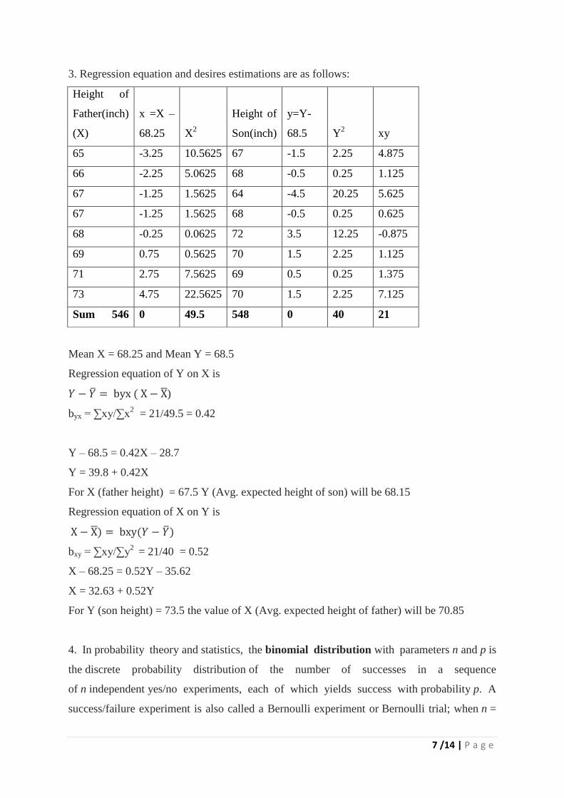
3. Regression equation and desires estimations are as follows:
Height of
Father(inch)
(X)
x =X –
68.25 X2
Height of
Son(inch)
y=Y-
68.5 Y2 xy
65 -3.25 10.5625 67 -1.5 2.25 4.875
66 -2.25 5.0625 68 -0.5 0.25 1.125
67 -1.25 1.5625 64 -4.5 20.25 5.625
67 -1.25 1.5625 68 -0.5 0.25 0.625
68 -0.25 0.0625 72 3.5 12.25 -0.875
69 0.75 0.5625 70 1.5 2.25 1.125
71 2.75 7.5625 69 0.5 0.25 1.375
73 4.75 22.5625 70 1.5 2.25 7.125
Sum 546 0 49.5 548 0 40 21
Mean X = 68.25 and Mean Y = 68.5
Regression equation of Y on X is
𝑌 − �̅� = byx ( X − X̅)
byx = ∑xy/∑x2
= 21/49.5 = 0.42
Y – 68.5 = 0.42X – 28.7
Y = 39.8 + 0.42X
For X (father height) = 67.5 Y (Avg. expected height of son) will be 68.15
Regression equation of X on Y is
X − X̅) = bxy(𝑌 − �̅�)
bxy = ∑xy/∑y2
= 21/40 = 0.52
X – 68.25 = 0.52Y – 35.62
X = 32.63 + 0.52Y
For Y (son height) = 73.5 the value of X (Avg. expected height of father) will be 70.85
4. In probability theory and statistics, the binomial distribution with parameters n and p is
the discrete probability distribution of the number of successes in a sequence
of n independent yes/no experiments, each of which yields success with probability p. A
success/failure experiment is also called a Bernoulli experiment or Bernoulli trial; when n =
8 /14 | P a g e
1, the binomial distribution is a Bernoulli distribution. The binomial distribution is the basis
for the popular binomial test of statistical significance.
The binomial distribution is frequently used to model the number of successes in a sample of
size n drawn with replacement from a population of size N. If the sampling is carried out
without replacement, the draws are not independent and so the resulting distribution is
a hypergeometric distribution, not a binomial one. However, for N much larger than n, the
binomial distribution is a good approximation, and widely used.
Hence an example of binomial distribution is as follows
Suppose we have n = 40 patients who will be receiving an experimental therapy which is
believed to be better than current treatments which historically have had a 5-year survival rate
of 20%, i.e. the probability of 5-year survival is
p = .20. Thus the number of patients out of 40 in our study surviving at least 5 years has a
binomial distribution, i.e. X ~ BIN(40,.20).
5. SYSTAT is a powerful statistical analysis and graphics software. Simplify your research
and enhance your publications with SYSTAT’s comprehensive suite of statistical functions
and brilliant 2D and 3D charts and graphs. In 1995 SYSTAT was sold to SPSS Inc., who
marketed the product to a scientific audience under the SPSS Science division. By 2002,
SPSS had changed its focus to business analytics and decided to sell SYSTAT to Cranes
Software in Bangalore, India. Cranes formed Systat Software, Inc. to market and distribute
SYSTAT in the US, and a number of other divisions for global distribution. The headquarters
are in Chicago, Illinois.
By 2005, SYSTAT was in its eleventh version having a revamped codebase completely
changed from Fortran into C++. Version 13 came out in 2009, with improvements in the user
interface and several new features.
Major functions of SYSTAT
ARCH and GARCH for Time Series
Best Subsets Regression
Confirmatory Factor Analysis
New data editor, gives faster computation
NEW SYSTAT 13 with Exact Tests Product
Major Elements of SYSTAT
File menu, Analysis, Data Sheet, Variable view, Help are major components of SYSTAT.
9 /14 | P a g e
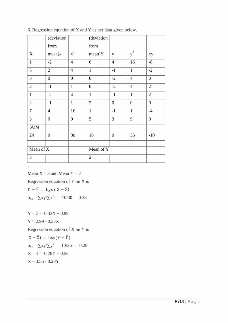
6. Regression equation of X and Y as per data given below.
X
(deviation
from
mean)x x2
(deviation
from
mean)Y y y2 xy
1 -2 4 6 4 16 -8
5 2 4 1 -1 1 -2
3 0 0 0 -2 4 0
2 -1 1 0 -2 4 2
1 -2 4 1 -1 1 2
2 -1 1 2 0 0 0
7 4 16 1 -1 1 -4
3 0 0 5 3 9 0
SUM
24 0 30 16 0 36 -10
Mean of X
Mean of Y
3
2
.
Mean X = 3 and Mean Y = 2
Regression equation of Y on X is
𝑌 − �̅� = byx ( X − X̅)
byx = ∑xy/∑x2
= -10/30 = -0.33
Y – 2 = -0.33X + 0.99
Y = 2.99 - 0.33X
Regression equation of X on Y is
X − X̅) = bxy(𝑌 − �̅�)
bxy = ∑xy/∑y2
= -10/36 = -0.28
X – 3 = -0.28Y + 0.56
X = 3.56 - 0.28Y
10 /14 | P a g e
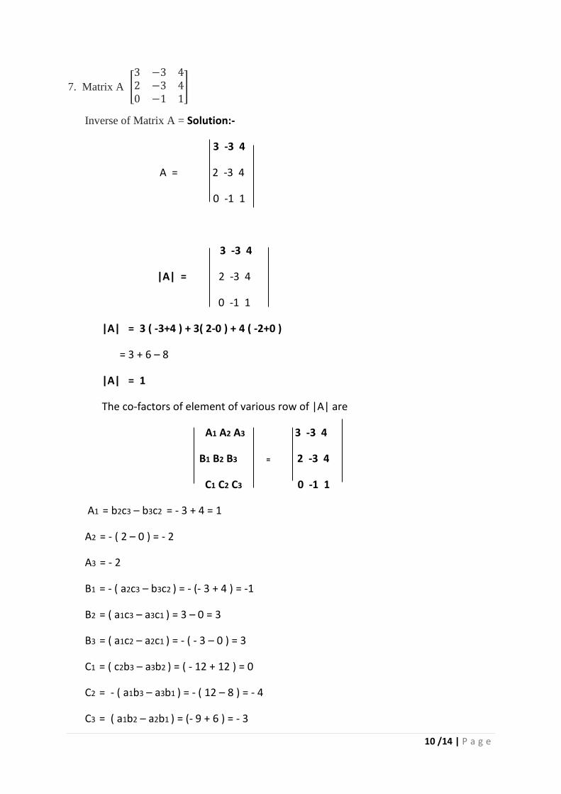
7. Matrix A [
3 −3 42 −3 40 −1 1
]
Inverse of Matrix A = Solution:-
3 -3 4
A = 2 -3 4
0 -1 1
3 -3 4
|A| = 2 -3 4
0 -1 1
|A| = 3 ( -3+4 ) + 3( 2-0 ) + 4 ( -2+0 )
= 3 + 6 – 8
|A| = 1
The co-factors of element of various row of |A| are
A1 A2 A3 3 -3 4
B1 B2 B3 = 2 -3 4
C1 C2 C3 0 -1 1
A1 = b2c3 – b3c2 = - 3 + 4 = 1
A2 = - ( 2 – 0 ) = - 2
A3 = - 2
B1 = - ( a2c3 – b3c2 ) = - (- 3 + 4 ) = -1
B2 = ( a1c3 – a3c1 ) = 3 – 0 = 3
B3 = ( a1c2 – a2c1 ) = - ( - 3 – 0 ) = 3
C1 = ( c2b3 – a3b2 ) = ( - 12 + 12 ) = 0
C2 = - ( a1b3 – a3b1 ) = - ( 12 – 8 ) = - 4
C3 = ( a1b2 – a2b1 ) = (- 9 + 6 ) = - 3
11 /14 | P a g e
1 -2 - 2
-1 3 3
0 -4 -3
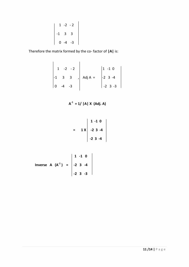
Therefore the matrix formed by the co- factor of |A| is:
1 -2 - 2 1 -1 0
-1 3 3 , Adj A = -2 3 -4
0 -4 -3 -2 3 -3
A-1 = 1/ |A| X (Adj. A)
1 -1 0
= 1 X -2 3 -4
-2 3 -4
1 -1 0
Inverse A (A-1 ) = -2 3 -4
-2 3 -3
12 /14 | P a g e
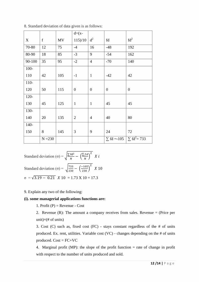
8. Standard deviation of data given is as follows:
X f MV
d=(x-
115)/10 d2 fd fd
2
70-80 12 75 -4 16 -48 192
80-90 18 85 -3 9 -54 162
90-100 35 95 -2 4 -70 140
100-
110 42 105 -1 1 -42 42
110-
120 50 115 0 0 0 0
120-
130 45 125 1 1 45 45
130-
140 20 135 2 4 40 80
140-
150 8 145 3 9 24 72
N =230
∑ fd =-105 ∑ fd2= 733
Standard deviation (σ) = √∑ fd2
𝑁− (
∑ 𝑓𝑑
𝑁)
2
𝑋 𝑖
Standard deviation (σ) = √733
230− (
−105
230)
2
𝑋 10
σ = √3.19 − 0.21 𝑋 10 = 1.73 X 10 = 17.3
9. Explain any two of the following:
(i). some managerial applications functions are:
1. Profit (P) = Revenue - Cost
2. Revenue (R): The amount a company receives from sales. Revenue = (Price per
unit)×(# of units)
3. Cost (C) such as, fixed cost (FC) - stays constant regardless of the # of units
produced. Ex. rent, utilities. Variable cost (VC) - changes depending on the # of units
produced. Cost = FC+VC
4. Marginal profit (MP): the slope of the profit function = rate of change in profit
with respect to the number of units produced and sold.
13 /14 | P a g e
5. Marginal cost (MC): the slope of the cost function.
6. Marginal revenue (MR): the slope of the revenue function.
7. A firm’s breakeven point occurs when P (x) = 0, or when R(x) = C(x).
Examples:
1. Total Cost, Revenue, and Profit- The profit a firm makes in a product is the
difference between the revenue (amount received in sales) and its costs (amount spent
by firm to produce the product). If x units are produced and sold, it is written: P(x) =
R(x)-C(x)
Where: P(x) = profit from x sale of units; R(x) = total revenue from sale of x units;
C(x) = total cost of production and sale of x units. Examples of fixed costs include
depreciation, rent, utilities, and so on. Variable costs, VC, are those directly related to
the number of units produced. Thus, the total cost is found by using the equation: C=
FC + VC.
(ii) Some illustrations of business applications of forecasting are as follows:
1. A telephone company may use forecast to customers equipment purchase enabling
it to cut cost and improve profitability
2. A gas company may use exponential smoothing model to forecast future demand
and overcome issues of over or under production eliminating shortage and
wastage.
3. Banks may use exponential smoothing to forecast loan demand.
4. Car manufacturing company may forecast demand of various models hence
optimizing the resources.
5. A hospital can use forecast to depute pathologist based on forecast of blood tests.
(iii). Utility of Time series in studying managerial problems
1. It helps in understanding the past behavior
2. Helps in planning future behaviors
3. It helps in evaluating current achievements and accomplishments
4. It facilitates comparisons.
(iv) Application of arithmetic and geometric progression:
14 /14 | P a g e
1. Manage volatility in investment: Geometric progression lowers volatility in
investment returns. Arithmetic and geometric averages serve different purposes and
only geometric averages will accurately reflect compounded investment returns.
Arithmetic averages will always over state investment returns unless there is zero
volatility. The greater the volatility the greater the difference will be between
arithmetic and geometric averages. When it comes to investment returns and
retirement planning it is compounded (geometric) averages that matter.
2. Retirement planning is another important area of application of geometric
progression. Following example explains the role of AP and GP
Arithmetic Average of a firm Total Returns in period 2000 – 2012 is:
(-9.2) + (-11.9) + (-22.1) + 28.7 + 10.9 + 4.9 +15.8 + 5.5 + (-37.0) + 26.5 + 15.1 +
2.1 + 15.8) / 13 = 4.89%
Geometric Average Total Returns (2000 – 2012):
[ .908 x .881 x .779 x 1.287 x 1.109 x 1.049 x 1.158 x 1.055 x .63 x 1.265 x 1.151 x
1.021 x 1.158) ^(1/13)] – 1 = 1.64%
Some problems that could be solved through AP and GP are:
a. In investigating different job opportunities, you find that firm A will start you at
$25,000 per year and guarantee you a raise of $1,200 each year while firm B will
start you at $28,000 per year but will guarantee you a raise of only $800 each
year. Over a period of 15 years, how much would you receive from each firm?
b. In investigating different job opportunities, you find that firm A will start you at
$25,000 per year and guarantee you a raise of $1,200 each year while firm B will
start you at $28,000 per year but will guarantee you a raise of only $800 each
year. Over a period of 15 years, how much would you receive from each firm?
c. In investigating different job opportunities, you find that firm A will start you at
$25,000 per year and guarantee you a raise of $1,200 each year while firm B will
start you at $28,000 per year but will guarantee you a raise of only $800 each
year. Over a period of 15 years, how much would you receive from each firm?