Embed Size (px)
Citation preview
Politecnico di Milano
Scuola di Ingegneria Industriale e dell’InformazioneCorso di Laurea Magistrale in Ingegneria Elettronica
Dipartimento di Elettronica, Informazione e Bioingegneria
MODEL AND CONTROL OF AN IN-WHEELBRUSHLESS MOTOR
Relatore: Prof. Giambattista GRUOSSO
Tesi di laurea di:Stefano BIANCHI Matr. 851038
Anno Accademico 2016–2017


For my family,who always supports meto reach my dreams. . .
-Stefano Bianchi -


Curiosity is all you need in life and if you are curious enough, you’regonna find your passions. And results who you get are just a logicalconsequence of how much passion you put on your life.
-Alex Zanardi-

Ringraziamenti
Questi sei anni universitari sono stati per me molto formativi, sia scolasticamente,che personalmente e umanamente. Nonostante una facoltà tecnica e scientifica basatasui numeri ho potuto capire che nella vita la differenza la fanno le persone cheincontriamo.
Vorrei quindi ringraziare i professori Giambattista Gruosso e Luca Bascetta per lapazienza con cui mi hanno seguito e per tutte le indicazioni necessarie per completarequesto lavoro.
Ringrazio anche Arturo Montúfar per gli insegnamenti nei mesi in cui abbiamocollaborato al progetto.
Vorrei ringraziare i miei genitori per essere sempre stati i miei sostenitori numerouno, per avermi dato la possibilità di arrivare fino a questo punto e perchè so che misupporteranno sempre e comunque; sperando che possa ripagare almeno in piccolaparte i vostri sacrifici rendendovi orgogliosi di me, e di ciò che grazie a voi ho potutorealizzare.
Un ringraziamento anche a tutta la mia famiglia: dai nonni, agli zii e ai cugini,ognuno di voi ha contribuito a suo modo al raggiungimento di questo mio traguardo.
Un grazie speciale alla mia sorellina, da quel 19 Giugno ne abbiamo passate tante,sono stati molti i litigi ma anche i bei momenti che ci hanno permesso di crescereinsieme. Sono contento di averti avuto al mio fianco tutti questi anni, e so che nonte lo dico abbastanza: ti voglio bene.
Tornando a casa ogni giorno dall’università è sempre bello trovare un amico che tisupporti e sopporti nei giorni peggiori o con cui festeggiare in quelli migliore, graziea tutti i miei coinquilini, sia a quelli attuali (Casone, Bomby, Zio Dam, Nico e Cat)che a quelli degli anni passati (Mathias, Salino, Marco e Rik).
Un gruppo di amici speciali, che fin da piccoli ti sono sempre stati accanto, èdifficile da trovare. Grazie per esserci sempre stati a Ricky, Spesly, Bonda, Pulkas,Montre e Manu.
Importante è stato anche l’imparare a lavorare in un team, ringrazio tutti colorocon cui ho condiviso attività e progetti: il gruppo degli animatori, le ragazze e iragazzi di CurtaTune, gli amici del karate e tutti i membri del Team DynamiΣ.

Abstract
The purpose of this thesis is to realize a MATLAB/Simulink model of an in-wheel motor: the system includes a motor inside the wheel, electronics necessaryto energize the motor and the control strategy to make it move at desired speed orwith a specific torque. There was applied two different control strategy on the wheel:one considering the motor with sinusoidal back electromotive Force and the otherconsidering the motor with Trapezoidal BEMF. The real motor, after a simple test,has proven to have sinusoidal BEMF. However both strategy can be still used.
Chapter 1 is about Brushless motor, it is explained its principle of operationand 2 kinds of motors are distinguished; furthermore control strategy most used areintroduced. In Chapter 2 it is analyzed the problem of calculation and estimation ofmotor’s parameters. After determination of parameters needed for simulation, theyare validated through some simulation. Chapter 3 is about field oriented control, itis shown the model and it is compared to experimental data. Established that themodel is an enough good approximation of the real system, parameters of controllersare calculated and compared. Chapter 4 is structured as Chapter 3 but relatively tothe Trapezoidal Control. Finally in Chapter 5 there is a short comparison betweencontrol strategy seen in chapters before to define which is better.
Results showed that Simulink model has a behavior very similar to the real motordespite simplifications mandatory in modeling process. This kind of result is validwith both control strategy. Comparisons between control strategy show that Focshould be preferable to 6-Step commutation, as expected by BEMF shapes. Moreconsideration can be done with the real motor: sensors in simulation (to read currentsand position) are considered ideal, in real word sensors introduce delays and noisenot yet considered in this simulation.

Sommario
L’obiettivo di questa tesi è quello di realizzare un modello in MATLAB/Simulinkdi una motoruota: un sistema che comprendente un motore brushless «in-wheel»,l’elettronica necessaria al funzionamento del motore e il sistema di controllo che cipermette di far ruotare la motoruota ad una determinata velocita o di applicareuna determinata coppia. Sono state attuate due diverse strategia di controllo con-siderando le due principali forme di forza controelettromotrice nei motori brushless:sinusoidale e trapezoidale. Il profilo della forza controelettromotrice del motore èstato verificato essere sinusoidale, ma entrambe le strategie di controllo rimangonoattuabili.
Il Capitolo 1 è dedicato al motore brushless: viene spiegato il principio di funzion-amento e vengono distinti i due tipi di motore brushless comunemente usati; vengonoinoltre presentate le due tecniche utilizzate per controllarli. Nel Capitolo 2 viene trat-tato il problema della determinazione e della stima dei parametri del motore. Dopoaver determinato i parametri necessari per la simulazione questi vengono validatianche tramite simulazione. Il Capitolo 3 è dedicato al sistema di controllo vettoriale,viene presentato il modello utilizzato e viene confrontato con i dati sperimentali. Unavolta appurato che il modello approssima correttamente il funzionamento del motorereale vengono calcolati i parametri dei controllori e simulati. Il Capitolo 4 è analogoal terzo ma la strategia di controllo utilizzata sarà invece quella trapezoidale. Infinenel capitolo 5 vengono confrontate le simulazioni utilizzando le 2 tecniche trattatenei capitoli precedenti per poter definire quale tecnica è più conveniente.
I risultati ottenuti mostrano che il modello Simulink ha un comportamento moltosimile a quello del motore reale nonostante le semplificazioni risultate obbligatorienella fase di modellazione. Questo è risultato valido con entrambe le tecniche dicontrollo. Il confronto tra queste in fase di simulazione mostra che è preferibile uncontrollo vettoriale, come ci si può aspettare conoscendo le forme delle forze con-troelettromotrici. Ulteriori considerazioni possono essere fatte utilizzando il motorereale: i sensori utilizzati nella simulazione (per correnti e posizione) sono ideali, isensori reali introducono invece ritardi e rumore non considerati.

Contents
Introduction 1
1 Brushless Motor 51.1 Operating principle . . . . . . . . . . . . . . . . . . . . . . . . . . . . 51.2 Trapezoidal Brushless Motor . . . . . . . . . . . . . . . . . . . . . . . 6
1.2.1 6-Step BLDC motor control . . . . . . . . . . . . . . . . . . . 61.2.2 Hall Effect Sensor . . . . . . . . . . . . . . . . . . . . . . . . 61.2.3 Torque generated by the Motor . . . . . . . . . . . . . . . . . 7
1.3 Sinusoidal Brushless Motor . . . . . . . . . . . . . . . . . . . . . . . 101.3.1 Torque generated by the Motor . . . . . . . . . . . . . . . . . 101.3.2 6-step Commutation applied on a sinusoidal motor . . . . . . 121.3.3 Current Control in a Brushless Motor . . . . . . . . . . . . . 12
2 Estimation and Validation of parameters 172.1 Resistance and Inductance of the Motor . . . . . . . . . . . . . . . . 172.2 Flux Linkage . . . . . . . . . . . . . . . . . . . . . . . . . . . . . . . 202.3 Friction of the Motor . . . . . . . . . . . . . . . . . . . . . . . . . . . 212.4 Inertia of the Motor . . . . . . . . . . . . . . . . . . . . . . . . . . . 212.5 Parameters with Load . . . . . . . . . . . . . . . . . . . . . . . . . . 25
2.5.1 Friction with Load . . . . . . . . . . . . . . . . . . . . . . . . 252.5.2 Inertia with Load . . . . . . . . . . . . . . . . . . . . . . . . . 26
3 Field Oriented Control Model 273.1 Simulink Model . . . . . . . . . . . . . . . . . . . . . . . . . . . . . . 27
3.1.1 Mechanical . . . . . . . . . . . . . . . . . . . . . . . . . . . . 273.1.2 Electrical . . . . . . . . . . . . . . . . . . . . . . . . . . . . . 283.1.3 Control . . . . . . . . . . . . . . . . . . . . . . . . . . . . . . 29
3.2 Simplified Model . . . . . . . . . . . . . . . . . . . . . . . . . . . . . 303.3 Validation of the Model . . . . . . . . . . . . . . . . . . . . . . . . . 323.4 Controller Parameters . . . . . . . . . . . . . . . . . . . . . . . . . . 39
3.4.1 Current Loop . . . . . . . . . . . . . . . . . . . . . . . . . . . 393.4.2 Speed Loop . . . . . . . . . . . . . . . . . . . . . . . . . . . . 41
i
Contents
4 Brushless DC Control Model 454.1 Simulink Model . . . . . . . . . . . . . . . . . . . . . . . . . . . . . . 45
4.1.1 Control . . . . . . . . . . . . . . . . . . . . . . . . . . . . . . 454.2 Simplified Model . . . . . . . . . . . . . . . . . . . . . . . . . . . . . 474.3 Validation of the Model . . . . . . . . . . . . . . . . . . . . . . . . . 494.4 Controller Parameters . . . . . . . . . . . . . . . . . . . . . . . . . . 63
4.4.1 Current Loop . . . . . . . . . . . . . . . . . . . . . . . . . . . 634.4.2 Speed Loop . . . . . . . . . . . . . . . . . . . . . . . . . . . . 65
5 Comparison between FOC and 6-Step 675.1 Speed Step Response Comparison . . . . . . . . . . . . . . . . . . . . 675.2 Comparison at Regime . . . . . . . . . . . . . . . . . . . . . . . . . . 695.3 Choise of Control Strategy . . . . . . . . . . . . . . . . . . . . . . . . 69
Conclusions 71
Bibliography 72
Bibliography 73
ii
List of Figures
1 The first Davenport motor . . . . . . . . . . . . . . . . . . . . . . . . 12 Division of electric motors . . . . . . . . . . . . . . . . . . . . . . . . 2
1.1 Brushless Motor . . . . . . . . . . . . . . . . . . . . . . . . . . . . . 51.2 Comparison BEMF in Sinusoidal and Trapezoidal Brushless Motor . 61.3 Currents flowing through coils with 6-step commutation sequence . 71.4 Windings in BLDC motor . . . . . . . . . . . . . . . . . . . . . . . . 81.5 Current and BEMF with 6-step commutation sequence . . . . . . . 91.6 6-step commutation applied on a sinusoidal motor . . . . . . . . . . . 131.7 Clarke Transformation . . . . . . . . . . . . . . . . . . . . . . . . . . 141.8 Park Transforamtion . . . . . . . . . . . . . . . . . . . . . . . . . . . 151.9 FOC Control Scheme . . . . . . . . . . . . . . . . . . . . . . . . . . . 16
2.1 Current Loop scheme to estimate Rphase and Lphase . . . . . . . . . . 172.2 Quadrature Current Step Response to calculate Rphase . . . . . . . . 182.3 Phase Currents with Rphase=186mΩ and Lphase=386µH . . . . . . . 192.4 Phase Currents with Rphase=80mΩ and Lphase=380µH . . . . . . . . 192.5 Phase Currents with Rphase=113.8mΩ and Lphase=79.7µH . . . . . . 202.6 Quadrature Currents Comparison to Validate Rphase and Lphase . . . 202.7 Polynomial curve that approximate the Friction of the Motor . . . . 212.8 Constant Acceleration of 3 A to compare Inertia . . . . . . . . . . . 242.9 Constant Acceleration with different Current Reference . . . . . . . . 242.10 Motor stopped by Friction to compare Inertia . . . . . . . . . . . . . 252.11 Polynomial curve that approximate the Friction of the Motor with Load 262.12 Constant Acceleration to Validate Inertia with Load . . . . . . . . . 26
3.1 Model of the System . . . . . . . . . . . . . . . . . . . . . . . . . . . 273.2 Friction Model . . . . . . . . . . . . . . . . . . . . . . . . . . . . . . 283.3 Model of Inverter . . . . . . . . . . . . . . . . . . . . . . . . . . . . . 293.4 Model of Controller . . . . . . . . . . . . . . . . . . . . . . . . . . . . 293.5 FOC and Speed Controller . . . . . . . . . . . . . . . . . . . . . . . . 303.6 Model of the System Simplified . . . . . . . . . . . . . . . . . . . . . 30
iii
List of Figures
3.7 Model of Controller Simplified . . . . . . . . . . . . . . . . . . . . . . 313.8 Comparison between complete and simplified models . . . . . . . . . 313.9 Phase currents step response to quadrature current reference . . . . . 323.10 Quadrature current step response to current reference . . . . . . . . 333.11 Speed step response to current reference 1A . . . . . . . . . . . . . . 333.12 Speed step response to current reference 2A . . . . . . . . . . . . . . 343.13 Speed step response to current reference 3A . . . . . . . . . . . . . . 343.14 Speed step response to current reference 3A with Load . . . . . . . . 353.15 Regime phase current with iq=2.5A . . . . . . . . . . . . . . . . . . . 353.16 Regime phase currents with iq=2.5A . . . . . . . . . . . . . . . . . . 363.17 Regime phase current with iq=2.8A . . . . . . . . . . . . . . . . . . . 363.18 Regime phase currents with iq=2.8A . . . . . . . . . . . . . . . . . . 373.19 Step Response 100 rpm . . . . . . . . . . . . . . . . . . . . . . . . . 383.20 Step Response 200 rpm . . . . . . . . . . . . . . . . . . . . . . . . . 383.21 Step Response 300 rpm . . . . . . . . . . . . . . . . . . . . . . . . . 393.22 Current control loop . . . . . . . . . . . . . . . . . . . . . . . . . . . 403.23 Step Response of quadrature current with different P and I values . . 413.24 Speed and Current Loop Nested . . . . . . . . . . . . . . . . . . . . . 413.25 Speed and Current Loop Nested . . . . . . . . . . . . . . . . . . . . . 423.26 Speed Step Response . . . . . . . . . . . . . . . . . . . . . . . . . . . 433.27 Speed Step Response . . . . . . . . . . . . . . . . . . . . . . . . . . . 43
4.1 Model of the System . . . . . . . . . . . . . . . . . . . . . . . . . . . 454.2 Model of Controller . . . . . . . . . . . . . . . . . . . . . . . . . . . . 464.3 Speed Control BLDC . . . . . . . . . . . . . . . . . . . . . . . . . . . 464.4 Speed Control BLDC with Current Loop . . . . . . . . . . . . . . . . 474.5 Model of the System Simplified . . . . . . . . . . . . . . . . . . . . . 474.6 Model of Controller Simplified . . . . . . . . . . . . . . . . . . . . . . 484.7 Current Phase with Duty Cycle 10% . . . . . . . . . . . . . . . . . . 504.8 Comparison Current Phases with Duty Cycle 10% . . . . . . . . . . 504.9 Voltage Phase with Duty Cycle 10% . . . . . . . . . . . . . . . . . . 514.10 Comparison of Voltage Phases with Duty Cycle 10% . . . . . . . . . 514.11 Tests with Duty Cycle 50% . . . . . . . . . . . . . . . . . . . . . . . 524.12 Tests with Duty Cycle 90% . . . . . . . . . . . . . . . . . . . . . . . 524.13 Current Phase with Duty Cycle 10% - With Load . . . . . . . . . . . 534.14 Comparison Current Phases with Duty Cycle 10% -With Load . . . 534.15 Voltage Phase with Duty Cycle 10% - With Load . . . . . . . . . . . 544.16 Comparison of Voltage Phases with Duty Cycle 10% - With Load . . 544.17 Tests with Duty Cycle 50% - With Load . . . . . . . . . . . . . . . . 554.18 Current Phase with Speed 100rpm . . . . . . . . . . . . . . . . . . . 56
iv
List of Figures
4.19 Comparison Current Phases with Speed 100 rpm . . . . . . . . . . . 564.20 Voltage Phase with Speed 100rpm . . . . . . . . . . . . . . . . . . . 574.21 Comparison of Voltage Phases with Speed 100 rpm . . . . . . . . . . 574.22 Tests with Speed 200 rpm . . . . . . . . . . . . . . . . . . . . . . . . 584.23 Tests with Speed 400 rpm . . . . . . . . . . . . . . . . . . . . . . . . 584.24 Current Phase with Speed 100rpm - With Load . . . . . . . . . . . . 594.25 Comparison Current Phases with Speed 100 rpm - With Load . . . . 594.26 Voltage Phase with Speed 100rpm - With Load . . . . . . . . . . . . 604.27 Comparison of Voltage Phases with Speed 100 rpm - With Load . . . 604.28 Tests with Speed 200 rpm - With Load . . . . . . . . . . . . . . . . . 614.29 Speed Step Response 100 rpm . . . . . . . . . . . . . . . . . . . . . . 624.30 Speed Step Response 200 rpm . . . . . . . . . . . . . . . . . . . . . . 624.31 Step Response of current with different P and I values . . . . . . . . 644.32 Speed Step Response with different PI Parameters . . . . . . . . . . 664.33 Speed Step Response with different PI Parameters - Detail . . . . . . 66
5.1 Speed Step Response with FOC and 6-Step . . . . . . . . . . . . . . 675.2 Torque during Step Response with FOC and 6-Step . . . . . . . . . . 685.3 Current phase during Speed Step Response with FOC and 6-Step . . 685.4 Torque at regime with FOC and 6-Step . . . . . . . . . . . . . . . . 695.5 Current Phase at regime with FOC and 6-Step . . . . . . . . . . . . 70
v

List of Figures
vi
Introduction
Electric motors provide the driving power for a large and still increasing part ofour modern industrial economy. The range of sizes and types of motors is large andthe number and diversity application continues to expand. [2]
The electric motor was first developed in the 1830s, around 30 years after thefirst battery.
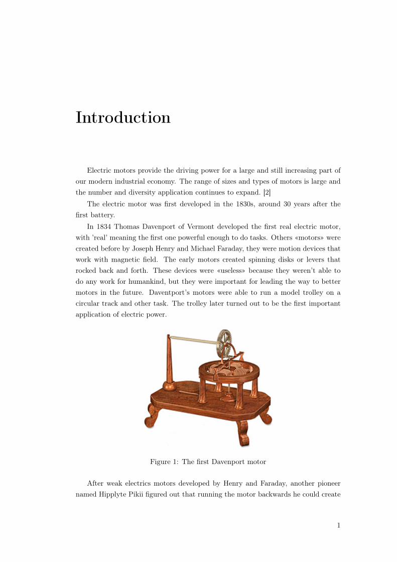
In 1834 Thomas Davenport of Vermont developed the first real electric motor,with ’real’ meaning the first one powerful enough to do tasks. Others «motors» werecreated before by Joseph Henry and Michael Faraday, they were motion devices thatwork with magnetic field. The early motors created spinning disks or levers thatrocked back and forth. These devices were «useless» because they weren’t able todo any work for humankind, but they were important for leading the way to bettermotors in the future. Daventport’s motors were able to run a model trolley on acircular track and other task. The trolley later turned out to be the first importantapplication of electric power.
Figure 1: The first Davenport motor
After weak electrics motors developed by Henry and Faraday, another pioneernamed Hipplyte Pikii figured out that running the motor backwards he could create
1
Introduction
pulses of electricity. By 1860s powerful generators were being developed. Withoutgenerators electrical industry could not begin because batteries were not an econom-ical way to power society’s needs.
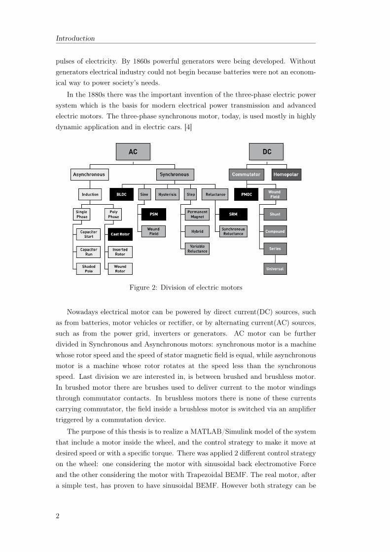
In the 1880s there was the important invention of the three-phase electric powersystem which is the basis for modern electrical power transmission and advancedelectric motors. The three-phase synchronous motor, today, is used mostly in highlydynamic application and in electric cars. [4]
Figure 2: Division of electric motors
Nowadays electrical motor can be powered by direct current(DC) sources, suchas from batteries, motor vehicles or rectifier, or by alternating current(AC) sources,such as from the power grid, inverters or generators. AC motor can be furtherdivided in Synchronous and Asynchronous motors: synchronous motor is a machinewhose rotor speed and the speed of stator magnetic field is equal, while asynchronousmotor is a machine whose rotor rotates at the speed less than the synchronousspeed. Last division we are interested in, is between brushed and brushless motor.In brushed motor there are brushes used to deliver current to the motor windingsthrough commutator contacts. In brushless motors there is none of these currentscarrying commutator, the field inside a brushless motor is switched via an amplifiertriggered by a commutation device.
The purpose of this thesis is to realize a MATLAB/Simulink model of the systemthat include a motor inside the wheel, and the control strategy to make it move atdesired speed or with a specific torque. There was applied 2 different control strategyon the wheel: one considering the motor with sinusoidal back electromotive Forceand the other considering the motor with Trapezoidal BEMF. The real motor, aftera simple test, has proven to have sinusoidal BEMF. However both strategy can be
2

Introduction
still used.In Chapter it 1 is explained the theory about Brushless motor and the way they
are controlled, including difference between Trapezoidal and Sinusoidal motor. InChapter 2 it is showed how parameters of the motor were calculated and estimated.In Chapter 3 is shown Field Oriented Control model and its validation with sometests. Chapter 4 is structured as Chapter 3 but relatively to the Trapezoidal Control.Finally in Chapter 5 there is a short comparison between these 2 strategy of control.
3

Introduction
4
Chapter 1
Brushless Motor
1.1 Operating principle
Figure 1.1: Brushless Motor
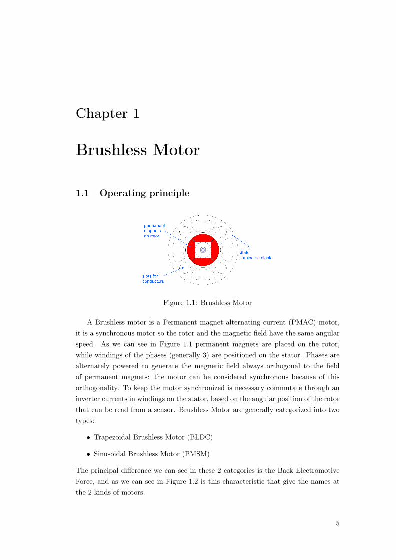
A Brushless motor is a Permanent magnet alternating current (PMAC) motor,it is a synchronous motor so the rotor and the magnetic field have the same angularspeed. As we can see in Figure 1.1 permanent magnets are placed on the rotor,while windings of the phases (generally 3) are positioned on the stator. Phases arealternately powered to generate the magnetic field always orthogonal to the fieldof permanent magnets: the motor can be considered synchronous because of thisorthogonality. To keep the motor synchronized is necessary commutate through aninverter currents in windings on the stator, based on the angular position of the rotorthat can be read from a sensor. Brushless Motor are generally categorized into twotypes:
• Trapezoidal Brushless Motor (BLDC)
• Sinusoidal Brushless Motor (PMSM)
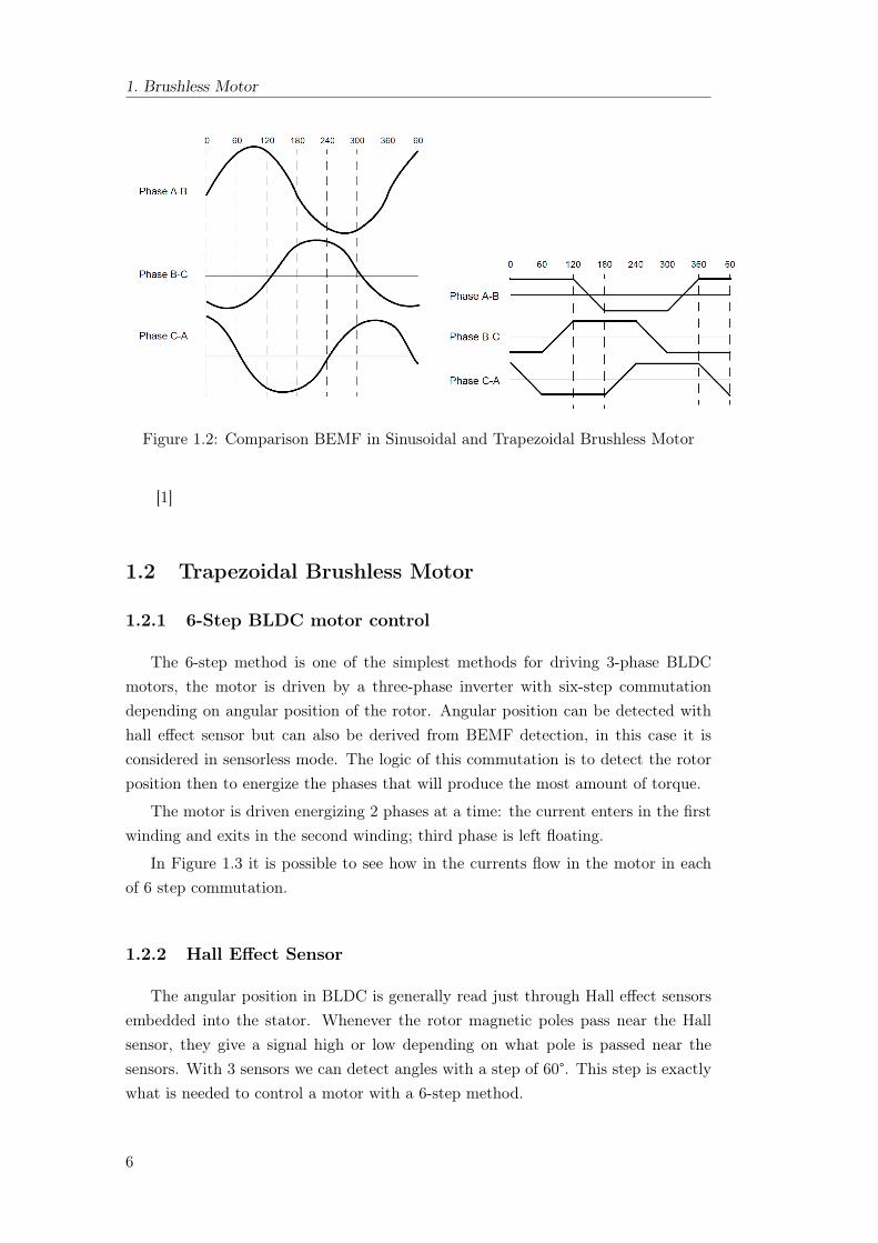
The principal difference we can see in these 2 categories is the Back ElectromotiveForce, and as we can see in Figure 1.2 is this characteristic that give the names atthe 2 kinds of motors.
5
1. Brushless Motor
Figure 1.2: Comparison BEMF in Sinusoidal and Trapezoidal Brushless Motor
[1]
1.2 Trapezoidal Brushless Motor
1.2.1 6-Step BLDC motor control
The 6-step method is one of the simplest methods for driving 3-phase BLDCmotors, the motor is driven by a three-phase inverter with six-step commutationdepending on angular position of the rotor. Angular position can be detected withhall effect sensor but can also be derived from BEMF detection, in this case it isconsidered in sensorless mode. The logic of this commutation is to detect the rotorposition then to energize the phases that will produce the most amount of torque.
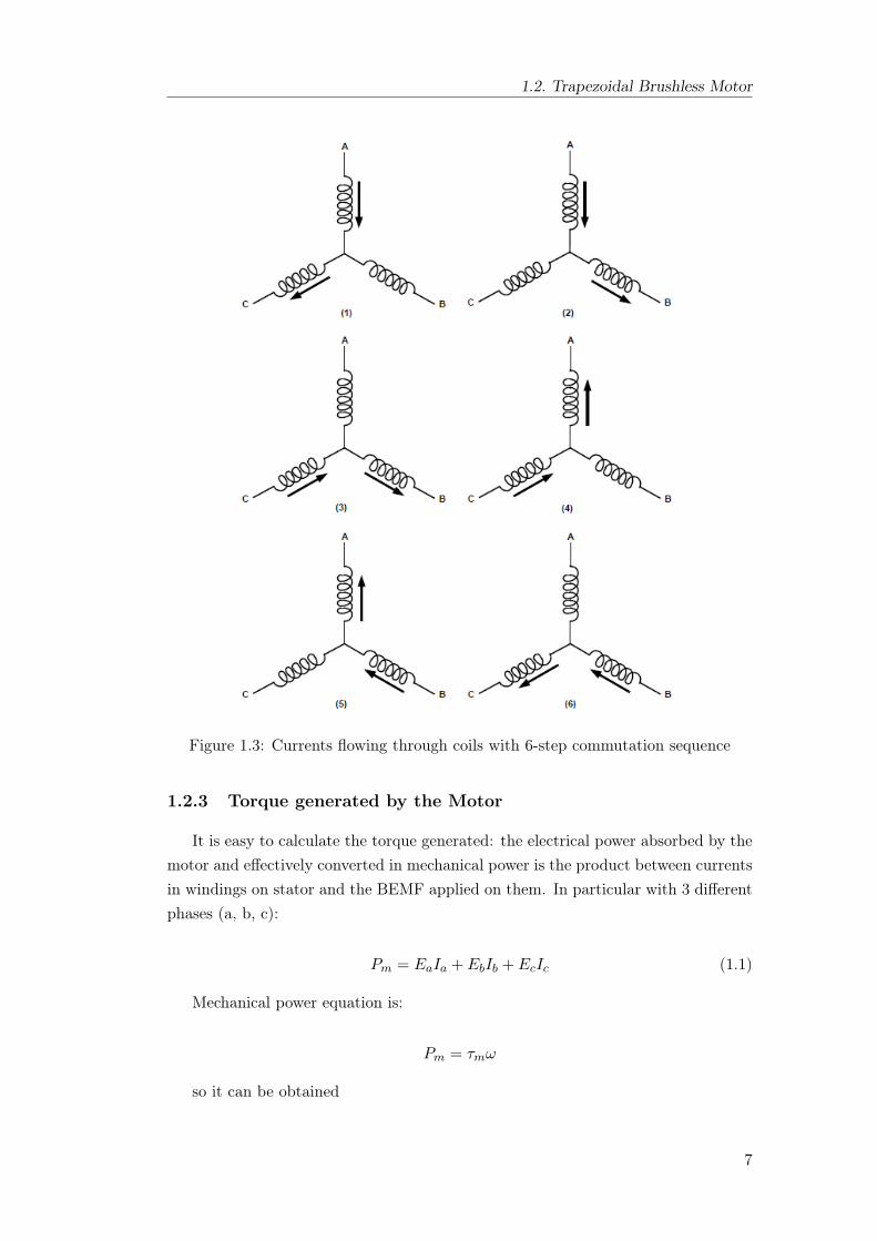
The motor is driven energizing 2 phases at a time: the current enters in the firstwinding and exits in the second winding; third phase is left floating.
In Figure 1.3 it is possible to see how in the currents flow in the motor in eachof 6 step commutation.
1.2.2 Hall Effect Sensor
The angular position in BLDC is generally read just through Hall effect sensorsembedded into the stator. Whenever the rotor magnetic poles pass near the Hallsensor, they give a signal high or low depending on what pole is passed near thesensors. With 3 sensors we can detect angles with a step of 60°. This step is exactlywhat is needed to control a motor with a 6-step method.
6
1.2. Trapezoidal Brushless Motor
Figure 1.3: Currents flowing through coils with 6-step commutation sequence
1.2.3 Torque generated by the Motor
It is easy to calculate the torque generated: the electrical power absorbed by themotor and effectively converted in mechanical power is the product between currentsin windings on stator and the BEMF applied on them. In particular with 3 differentphases (a, b, c):
Pm = EaIa + EbIb + EcIc (1.1)
Mechanical power equation is:
Pm = τmω
so it can be obtained
7
1. Brushless Motor
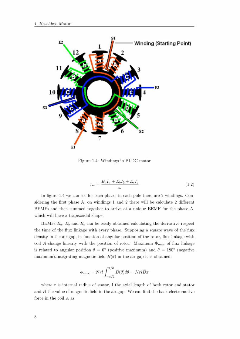
Figure 1.4: Windings in BLDC motor
τm =EaIa + EbIb + EcIc
ω(1.2)
In figure 1.4 we can see for each phase, in each pole there are 2 windings. Con-sidering the first phase A, on windings 1 and 2 there will be calculate 2 differentBEMFs and then summed together to arrive at a unique BEMF for the phase A,which will have a trapezoidal shape.
BEMFs Ea, Eb and Ec can be easily obtained calculating the derivative respectthe time of the flux linkage with every phase. Supposing a square wave of the fluxdensity in the air gap, in function of angular position of the rotor, flux linkage withcoil A change linearly with the position of rotor. Maximum Φmax of flux linkageis related to angular position θ = 0 (positive maximum) and θ = 180 (negativemaximum).Integrating magnetic field B(θ) in the air gap it is obtained:
φmax = Nrl
∫ π/2
−π/2B(θ)dθ = NrlBπ
where r is internal radius of stator, l the axial length of both rotor and statorand B the value of magnetic field in the air gap. We can find the back electromotiveforce in the coil A as:
8
1.2. Trapezoidal Brushless Motor
EA = −dφm1
dt= −dφmi
dθ
dθ
dt= −ωdφm1
dθ
Expressing the derivative of the flux linkage respect the angle in function ofmaximum flux linkage it is obtained a square wave BEMF, which amplitude is:
EA =2φmaxπ|ω|
BEMF in coil a has the same expression but it is out of phase of 30°. When bothcoils are connected in series, the resulting BEMF will become trapezoidal. With realwindings it is obtained for each phase a trapezoidal BEMF Ei(θ), with amplitude
Ei =4φmaxpi|ω|
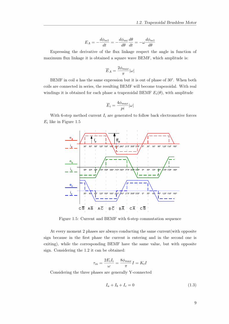
With 6-step method current Ii are generated to follow back electromotive forcesEi like in Figure 1.5
Figure 1.5: Current and BEMF with 6-step commutation sequence
At every moment 2 phases are always conducting the same current(with oppositesign because in the first phase the current is entering and in the second one isexiting), while the corresponding BEMF have the same value, but with oppositesign. Considering the 1.2 it can be obtained:
τm =2EiIiω
=8φmaxπ
I = KtI
Considering the three phases are generally Y-connected
Ia + Ib + Ic = 0 (1.3)
9
1. Brushless Motor
the brushless motor model, relatively of electrical parameters, is defined by theequation 1.3 and by the following:
Va
Vb
Vc
=
R 0 0
0 R 0
0 0 R
Ia
Ib
Ic
+d
dt
La Mab Mac
Mba Lb Mbc
Mca Mcb Lc
Ia
Ib
Ic
+
Ea
Eb
Ec
+
Vn
Vn
Vn
(1.4)
where Vi are voltages applied to phases having as reference the ground of theinverter, Vn is the potential of neutral, R is the phase resistance, Ei are the backelectromotive force and Li , Mij are respectively auto and mutual inductances ofphase. Assuming reluctances of motors don’t change with the angle, so Li are equaland the same for Mij , the considered equation 1.4 becomes: Va
Vb
Vc
= R
Ia
Ib
Ic
+ Ld
dt
Ia
Ib
Ic
+
Ea
Eb
Ec
+
Vn
Vn
Vn
(1.5)
where L = Li −Mij .
1.3 Sinusoidal Brushless Motor
1.3.1 Torque generated by the Motor
Principal difference between a brushless trapezoidal motor and a sinusoidal oneconsist in the different shape function obtained in the back electromotive forces. Inboth cases the BEMFs can be expressed as a product of the angular speed by a shapefunction Ki(θ), so:
Ei = ωKi(θ)
Configuring appropriately permanent magnets on the rotor is possible to obtaina sinusoidal distribution of the magnetic field, having the direction of maximum am-plitude which rotate at the speed of the rotor. Considering the direction of maximumamplitude of the magnetic field as a reference mobile axis to measure the angles:
B(ϕ, θ) = Bcos(ϕ− θ)
where ϕ represent a generic point in the air gap and θ is the rotation of the rotor.Considering a sinusoidal distribution for conductors of each phase, in which in
an infinitesimal angle dϕ are contained a number of conductor
dn =Ns
2sin(ϕ)dϕ
10
1.3. Sinusoidal Brushless Motor
where Ns is the number of turns in the coil. We can calculate the flux linkage φmwith the coil composed by dn conductor, furthermore we consider conductors returnwith an angle −ϕ
φm =
∫ ϕ
−ϕB(σ, θ)rldσ = 2Brlsinϕcosθ
Back electromotive force dE inducted by the coil composed by dn conductorswill be
dE = −dφmdt
dn = BrlωNssin2ϕsinθdϕ
Overall back electromotive force E will be
E =
∫ π
0dE = ω
BrlNSπ
2sinθ = ωKsinθ
Three phase have 23π of phase displacement, and considering the generic case
having p polar pairs:
Ka(α) = pKsin(pθ) = pKsin(α)
Kb(α) = pKsin(pθ − 2π/3) = pKsin(α− 2π/3)
Kc(α) = pKsin(pθ − 4π/3) = pKsin(α− 4π/3)
To obtain a constant torque independent from the angle we have to impose cur-rents
Ia = Ia(α) = Isin(α)
Ib = Ib(α) = Isin(α− 2π/3)
Ic = Ic(α) = Isin(α− 4π/3)
Considering the equation 1.2 :
τm = pKIsin2α+ pKIsin2(α− 2π/3) + pKIsin2(α− 4π/3) =2
3pKI = KtI
Dynamic of electrical quantities is still descripted by equations 1.3 and 1.5 .
11
1. Brushless Motor
1.3.2 6-step Commutation applied on a sinusoidal motor
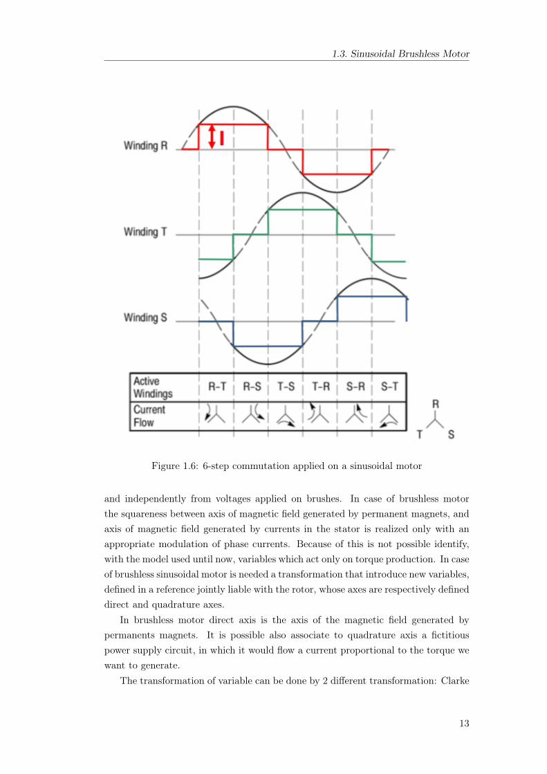
As it was said before 6-step commutation is an easy way to control a BLDCmotor, but it is possible to apply this method to a sinusoidal motor. As we can seelater the torque will present a ripple due to we are considering trapezoidal a BEMFthat actually is Sinusoidal. [8]
In Figure 1.6 we can see the current applied on phases is the same applied onFigure 1.5, but the BEMF is sinusoidal, in both cases we apply a constant currentin the 120° where BEMF is maximum.
Let’s try to calculate the torque from each phase in a period of 60°. We canconsider phases A and B conducting, and phase C floating, with positive value inphase A:
τa = pKIsin(θ)
τb = pK(−I)sin(θ − 23π)
τc = 0
τ = pKI
[sin(θ)− sin(θ − 2
3π)
]= −√
3sin(θ +π
6)KI (1.6)
We can obtainτmax =
√3pKI
τavg = 0.995τmax
and
τmin = 0.866τmax
1.3.3 Current Control in a Brushless Motor
In three phase brushless motor we have three different currents, one in each phase,we want to control, but considering the equation 1.3 we know the 3 phase currentsaren’t independent to each other. So it’s enough control 2 of them and the third onewill be uniquely determined by the Y -connection of the motor’s phases.
In case of digital control is preferred, after an appropriate transformation ofvariables, change the model of the motor in order to eliminate the dependence fromthe electrical angle α. This technic is called Field Oriented Control.
From the point of view of control, brushed motors are the better machine: themain advantage is guaranteed by a situation of complete magnetic decoupling. It canbe defined a polar axis, defined by permanent magnets, and a quadrature axis definedby magnetic field generated by armature currents. Furthermore these 2 axes arealways orthogonal, independently to relative positon of the rotor respect the stator,
12
1.3. Sinusoidal Brushless Motor
Figure 1.6: 6-step commutation applied on a sinusoidal motor
and independently from voltages applied on brushes. In case of brushless motorthe squareness between axis of magnetic field generated by permanent magnets, andaxis of magnetic field generated by currents in the stator is realized only with anappropriate modulation of phase currents. Because of this is not possible identify,with the model used until now, variables which act only on torque production. In caseof brushless sinusoidal motor is needed a transformation that introduce new variables,defined in a reference jointly liable with the rotor, whose axes are respectively defineddirect and quadrature axes.
In brushless motor direct axis is the axis of the magnetic field generated bypermanents magnets. It is possible also associate to quadrature axis a fictitiouspower supply circuit, in which it would flow a current proportional to the torque wewant to generate.
The transformation of variable can be done by 2 different transformation: Clarke
13
1. Brushless Motor
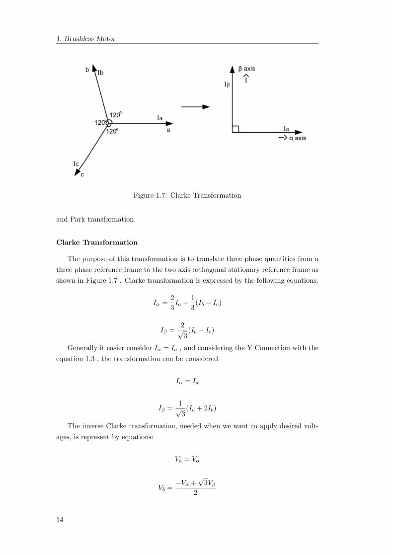
Figure 1.7: Clarke Transformation
and Park transformation.
Clarke Transformation
The purpose of this transformation is to translate three phase quantities from athree phase reference frame to the two axis orthogonal stationary reference frame asshown in Figure 1.7 . Clarke transformation is expressed by the following equations:
Iα =2
3Ia −
1
3(Ib − Ic)
Iβ =2√3
(Ib − Ic)
Generally it easier consider Iα = Ia , and considering the Y Connection with theequation 1.3 , the transformation can be considered
Iα = Ia
Iβ =1√3
(Ia + 2Ib)
The inverse Clarke transformation, needed when we want to apply desired volt-ages, is represent by equations:
Va = Vα
Vb =−Vα +
√3Vβ
2
14
1.3. Sinusoidal Brushless Motor
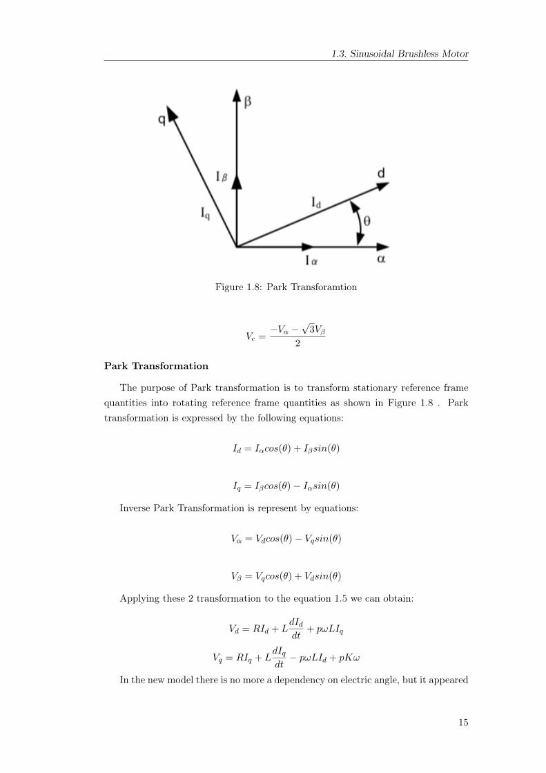
Figure 1.8: Park Transforamtion
Vc =−Vα −
√3Vβ
2
Park Transformation
The purpose of Park transformation is to transform stationary reference framequantities into rotating reference frame quantities as shown in Figure 1.8 . Parktransformation is expressed by the following equations:
Id = Iαcos(θ) + Iβsin(θ)
Iq = Iβcos(θ)− Iαsin(θ)
Inverse Park Transformation is represent by equations:
Vα = Vdcos(θ)− Vqsin(θ)
Vβ = Vqcos(θ) + Vdsin(θ)
Applying these 2 transformation to the equation 1.5 we can obtain:
Vd = RId + LdIddt
+ pωLIq
Vq = RIq + LdIqdt− pωLId + pKω
In the new model there is no more a dependency on electric angle, but it appeared
15
1. Brushless Motor
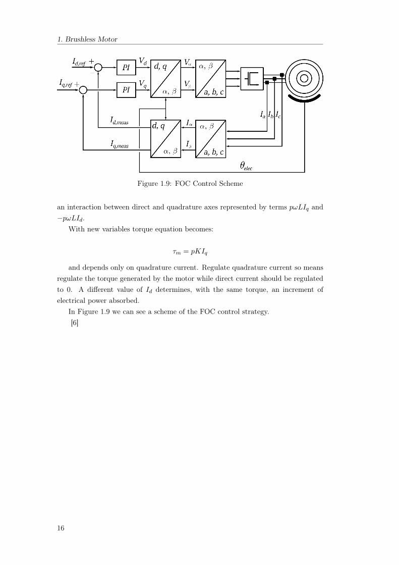
Figure 1.9: FOC Control Scheme
an interaction between direct and quadrature axes represented by terms pωLIq and−pωLId.
With new variables torque equation becomes:
τm = pKIq
and depends only on quadrature current. Regulate quadrature current so meansregulate the torque generated by the motor while direct current should be regulatedto 0. A different value of Id determines, with the same torque, an increment ofelectrical power absorbed.
In Figure 1.9 we can see a scheme of the FOC control strategy.[6]
16
Chapter 2
Estimation and Validation ofparameters
2.1 Resistance and Inductance of the Motor
From previous experiments we know values of theRphase=80mΩ and Lphase=360µHbut calculating the same values from the vedder software we obtain 2 different values:Rphase=113.8mΩ and Lphase=79,7µH [5] [3]
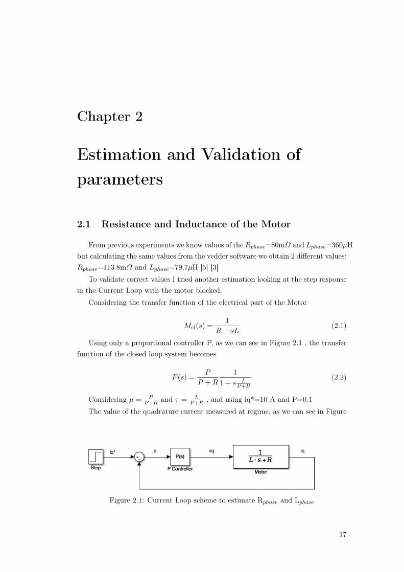
To validate correct values I tried another estimation looking at the step responsein the Current Loop with the motor blocked.
Considering the transfer function of the electrical part of the Motor
Mel(s) =1
R+ sL(2.1)
Using only a proportional controller P, as we can see in Figure 2.1 , the transferfunction of the closed loop system becomes
F (s) =P
P +R
1
1 + s LP+R
(2.2)
Considering µ = PP+R and τ = L
P+R , and using iq*=10 A and P=0.1
The value of the quadrature current measured at regime, as we can see in Figure
Figure 2.1: Current Loop scheme to estimate Rphase and Lphase
17
2. Estimation and Validation of parameters
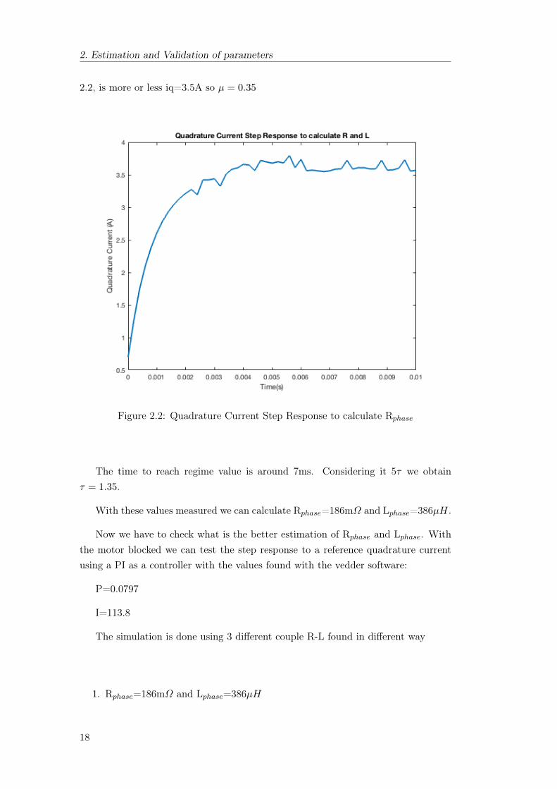
2.2, is more or less iq=3.5A so µ = 0.35
Figure 2.2: Quadrature Current Step Response to calculate Rphase
The time to reach regime value is around 7ms. Considering it 5τ we obtainτ = 1.35.
With these values measured we can calculate Rphase=186mΩ and Lphase=386µH.
Now we have to check what is the better estimation of Rphase and Lphase. Withthe motor blocked we can test the step response to a reference quadrature currentusing a PI as a controller with the values found with the vedder software:
P=0.0797
I=113.8
The simulation is done using 3 different couple R-L found in different way
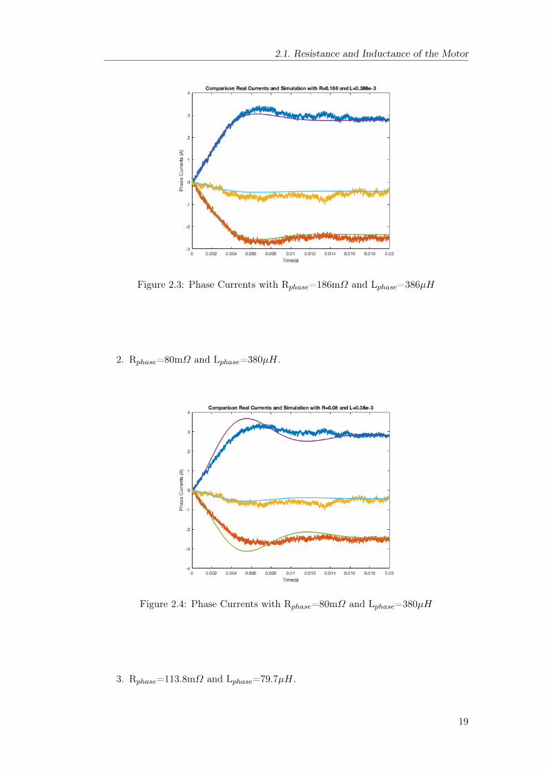
1. Rphase=186mΩ and Lphase=386µH
18
2.1. Resistance and Inductance of the Motor
Figure 2.3: Phase Currents with Rphase=186mΩ and Lphase=386µH
2. Rphase=80mΩ and Lphase=380µH.
Figure 2.4: Phase Currents with Rphase=80mΩ and Lphase=380µH
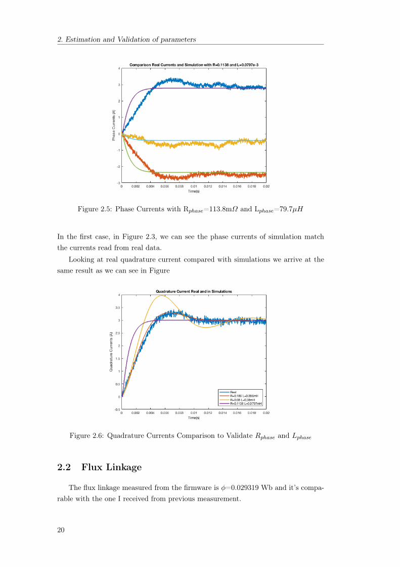
3. Rphase=113.8mΩ and Lphase=79.7µH.
19
2. Estimation and Validation of parameters
Figure 2.5: Phase Currents with Rphase=113.8mΩ and Lphase=79.7µH
In the first case, in Figure 2.3, we can see the phase currents of simulation matchthe currents read from real data.
Looking at real quadrature current compared with simulations we arrive at thesame result as we can see in Figure
Figure 2.6: Quadrature Currents Comparison to Validate Rphase and Lphase
2.2 Flux Linkage
The flux linkage measured from the firmware is φ=0.029319 Wb and it’s compa-rable with the one I received from previous measurement.
20
2.3. Friction of the Motor
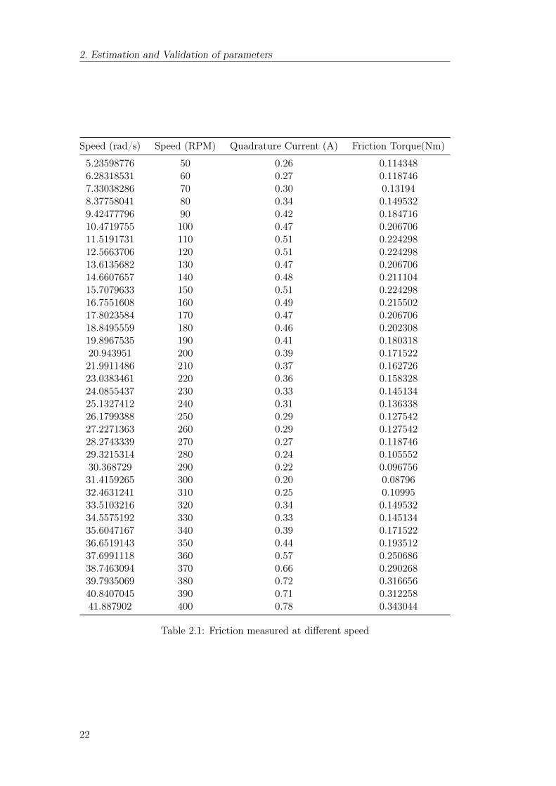
2.3 Friction of the Motor
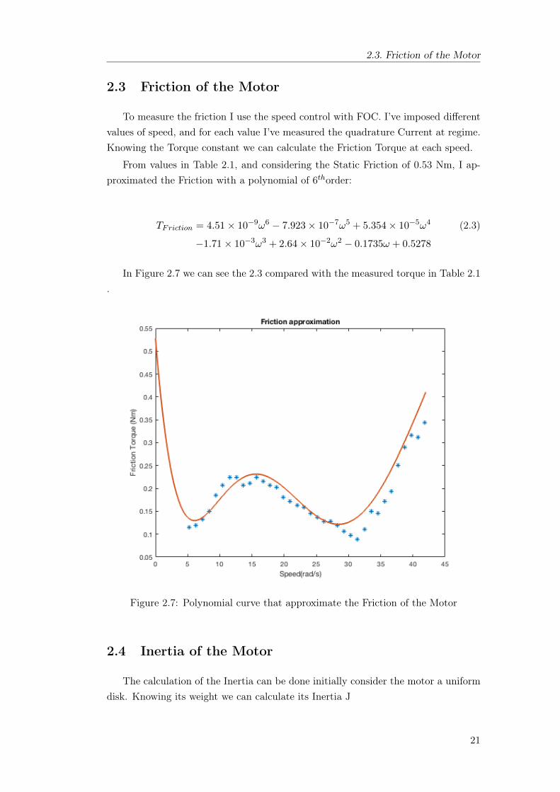
To measure the friction I use the speed control with FOC. I’ve imposed differentvalues of speed, and for each value I’ve measured the quadrature Current at regime.Knowing the Torque constant we can calculate the Friction Torque at each speed.
From values in Table 2.1, and considering the Static Friction of 0.53 Nm, I ap-proximated the Friction with a polynomial of 6thorder:
TFriction = 4.51× 10⁻⁹ω6 − 7.923× 10⁻⁷ω5 + 5.354× 10⁻⁵ω4 (2.3)
−1.71× 10⁻³ω3 + 2.64× 10⁻²ω2 − 0.1735ω + 0.5278
In Figure 2.7 we can see the 2.3 compared with the measured torque in Table 2.1.
Figure 2.7: Polynomial curve that approximate the Friction of the Motor
2.4 Inertia of the Motor
The calculation of the Inertia can be done initially consider the motor a uniformdisk. Knowing its weight we can calculate its Inertia J
21
2. Estimation and Validation of parameters
Speed (rad/s) Speed (RPM) Quadrature Current (A) Friction Torque(Nm)
5.23598776 50 0.26 0.1143486.28318531 60 0.27 0.1187467.33038286 70 0.30 0.131948.37758041 80 0.34 0.1495329.42477796 90 0.42 0.18471610.4719755 100 0.47 0.20670611.5191731 110 0.51 0.22429812.5663706 120 0.51 0.22429813.6135682 130 0.47 0.20670614.6607657 140 0.48 0.21110415.7079633 150 0.51 0.22429816.7551608 160 0.49 0.21550217.8023584 170 0.47 0.20670618.8495559 180 0.46 0.20230819.8967535 190 0.41 0.18031820.943951 200 0.39 0.17152221.9911486 210 0.37 0.16272623.0383461 220 0.36 0.15832824.0855437 230 0.33 0.14513425.1327412 240 0.31 0.13633826.1799388 250 0.29 0.12754227.2271363 260 0.29 0.12754228.2743339 270 0.27 0.11874629.3215314 280 0.24 0.10555230.368729 290 0.22 0.09675631.4159265 300 0.20 0.0879632.4631241 310 0.25 0.1099533.5103216 320 0.34 0.14953234.5575192 330 0.33 0.14513435.6047167 340 0.39 0.17152236.6519143 350 0.44 0.19351237.6991118 360 0.57 0.25068638.7463094 370 0.66 0.29026839.7935069 380 0.72 0.31665640.8407045 390 0.71 0.31225841.887902 400 0.78 0.343044
Table 2.1: Friction measured at different speed
22
2.4. Inertia of the Motor
J =mr2
2(2.4)
In this way J result to be J=0.046 Kgm2
But this is just a first estimation based on the uniform distribution of the massof the motor. This is not true so to calculate the motor we can try to impose aconstant Torque to have a constant acceleration and we can detect the Inertia.
We know that
Jdω
dt= T − Tfriction (2.5)
So during an acceleration we can find different
Ji =(T − Tfriction) ×∆t
ωi − ωi−1(2.6)
And we can calculate the mean J
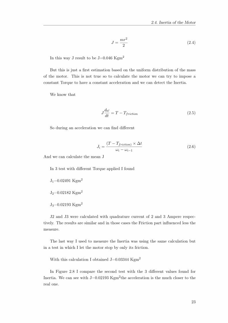
In 3 test with different Torque applied I found
J1=0.02491 Kgm2
J2=0.02182 Kgm2
J3=0.02193 Kgm2
J2 and J3 were calculated with quadrature current of 2 and 3 Ampere respec-tively. The results are similar and in those cases the Friction part influenced less themeasure.
The last way I used to measure the Inertia was using the same calculation butin a test in which I let the motor stop by only its friction.
With this calculation I obtained J=0.03344 Kgm2
In Figure 2.8 I compare the second test with the 3 different values found forInertia. We can see with J=0.02193 Kgm2the acceleration is the much closer to thereal one.
23
2. Estimation and Validation of parameters
Figure 2.8: Constant Acceleration of 3 A to compare Inertia
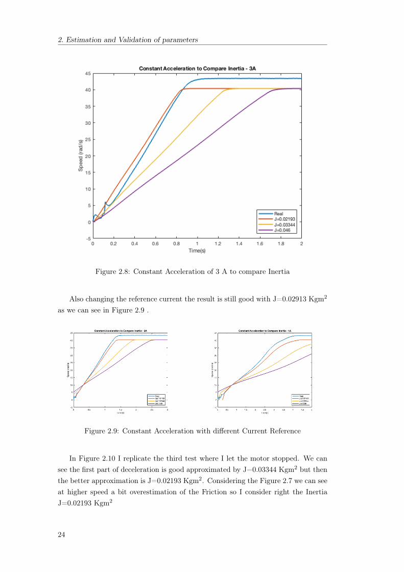
Also changing the reference current the result is still good with J=0.02913 Kgm2
as we can see in Figure 2.9 .
Figure 2.9: Constant Acceleration with different Current Reference
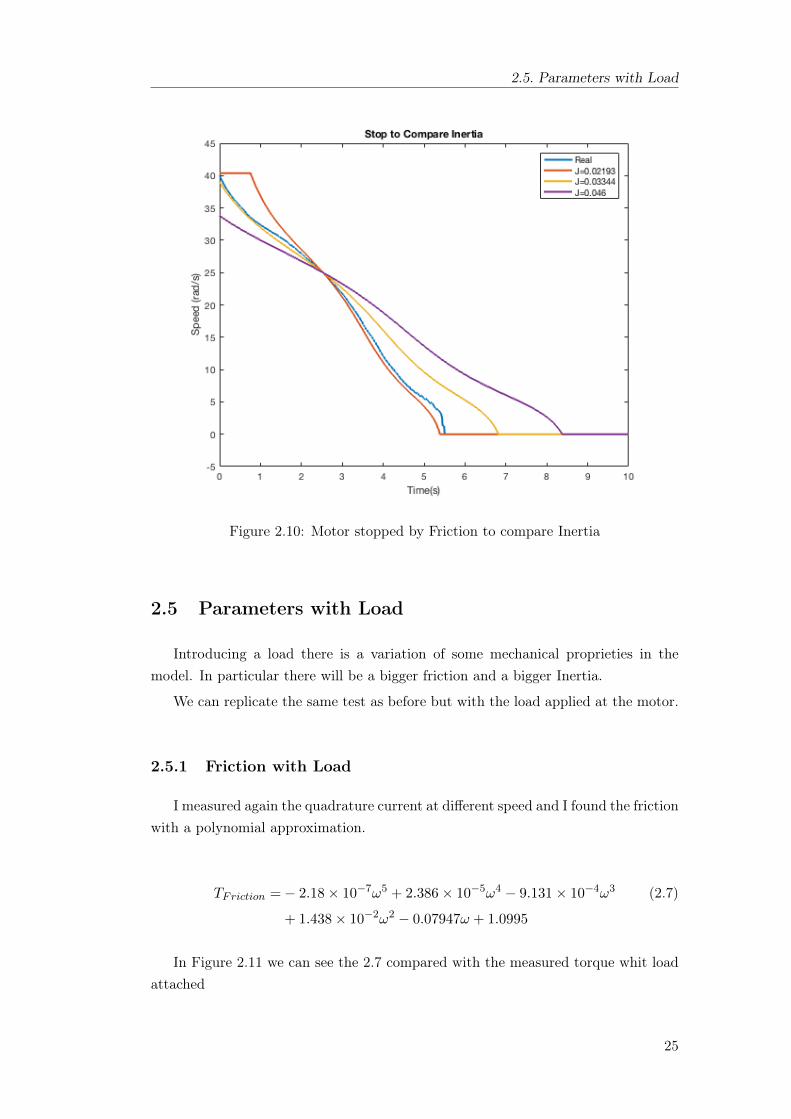
In Figure 2.10 I replicate the third test where I let the motor stopped. We cansee the first part of deceleration is good approximated by J=0.03344 Kgm2 but thenthe better approximation is J=0.02193 Kgm2. Considering the Figure 2.7 we can seeat higher speed a bit overestimation of the Friction so I consider right the InertiaJ=0.02193 Kgm2
24
2.5. Parameters with Load
Figure 2.10: Motor stopped by Friction to compare Inertia
2.5 Parameters with Load
Introducing a load there is a variation of some mechanical proprieties in themodel. In particular there will be a bigger friction and a bigger Inertia.
We can replicate the same test as before but with the load applied at the motor.
2.5.1 Friction with Load
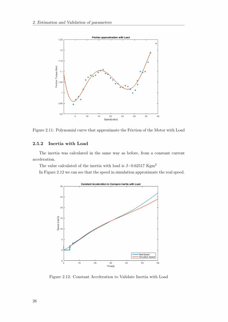
I measured again the quadrature current at different speed and I found the frictionwith a polynomial approximation.
TFriction =− 2.18× 10⁻⁷ω5 + 2.386× 10⁻⁵ω4 − 9.131× 10⁻⁴ω3 (2.7)
+ 1.438× 10⁻²ω2 − 0.07947ω + 1.0995
In Figure 2.11 we can see the 2.7 compared with the measured torque whit loadattached
25
2. Estimation and Validation of parameters
Figure 2.11: Polynomial curve that approximate the Friction of the Motor with Load
2.5.2 Inertia with Load
The inertia was calculated in the same way as before, from a constant currentacceleration.
The value calculated of the inertia with load is J=0.62517 Kgm2
In Figure 2.12 we can see that the speed in simulation approximate the real speed.
Figure 2.12: Constant Acceleration to Validate Inertia with Load
26
Chapter 3
Field Oriented Control Model
3.1 Simulink Model
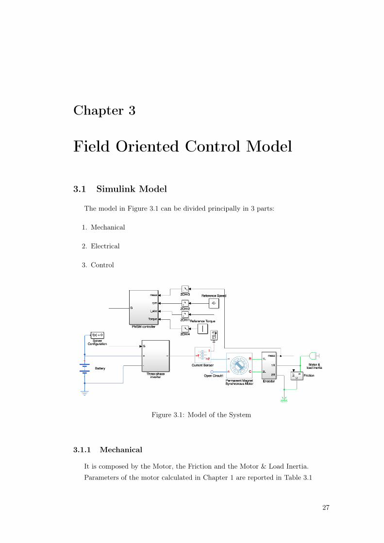
The model in Figure 3.1 can be divided principally in 3 parts:
1. Mechanical
2. Electrical
3. Control
Figure 3.1: Model of the System
3.1.1 Mechanical
It is composed by the Motor, the Friction and the Motor & Load Inertia.
Parameters of the motor calculated in Chapter 1 are reported in Table 3.1
27
3. Field Oriented Control Model
Rphase 186mΩ
Lphase 386µH
Flux Linkage φ 0.029319 Wb
Number of poles N 10
Inertia J 0.02193 Kgm2
Table 3.1: Parameters of the Motor
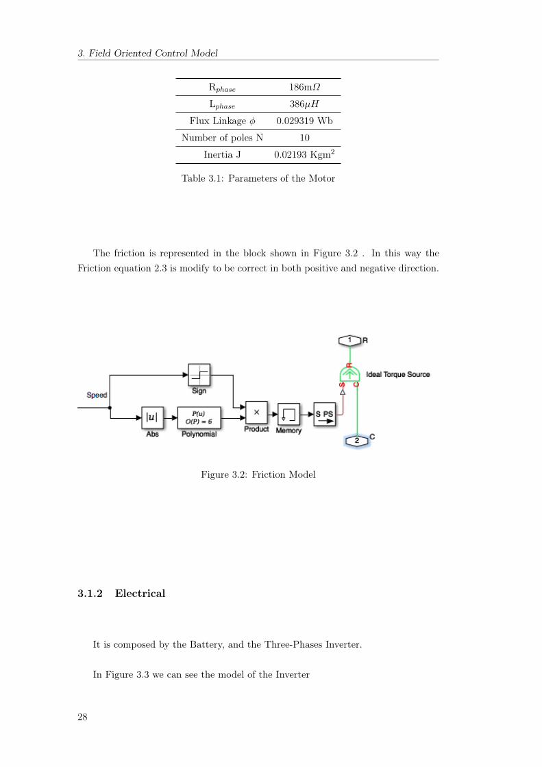
The friction is represented in the block shown in Figure 3.2 . In this way theFriction equation 2.3 is modify to be correct in both positive and negative direction.
Figure 3.2: Friction Model
3.1.2 Electrical
It is composed by the Battery, and the Three-Phases Inverter.
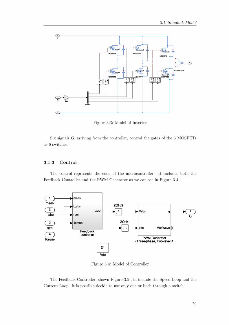
In Figure 3.3 we can see the model of the Inverter
28
3.1. Simulink Model
Figure 3.3: Model of Inverter
Six signals G, arriving from the controller, control the gates of the 6 MOSFETsas 6 switches.
3.1.3 Control
The control represents the code of the microcontroller. It includes both theFeedback Controller and the PWM Generator as we can see in Figure 3.4 .
Figure 3.4: Model of Controller
The Feedback Controller, shown Figure 3.5 , in include the Speed Loop and theCurrent Loop. It is possible decide to use only one or both through a switch.
29
3. Field Oriented Control Model
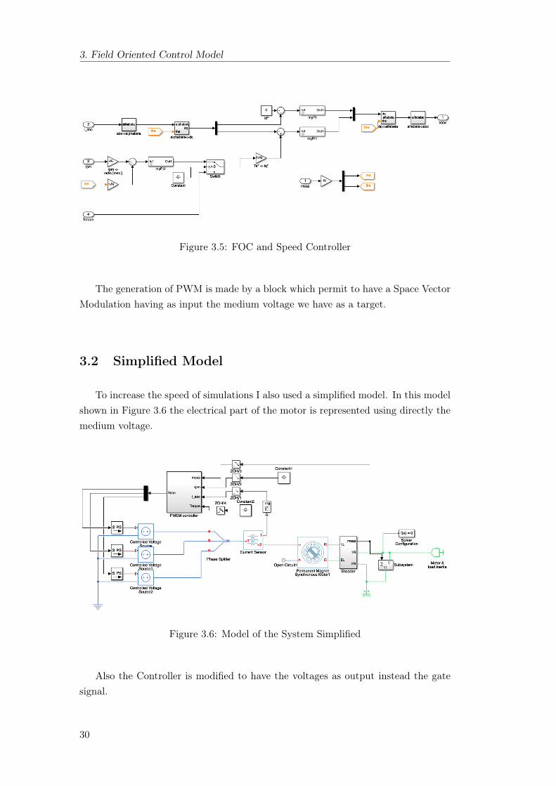
Figure 3.5: FOC and Speed Controller
The generation of PWM is made by a block which permit to have a Space VectorModulation having as input the medium voltage we have as a target.
3.2 Simplified Model
To increase the speed of simulations I also used a simplified model. In this modelshown in Figure 3.6 the electrical part of the motor is represented using directly themedium voltage.
Figure 3.6: Model of the System Simplified
Also the Controller is modified to have the voltages as output instead the gatesignal.
30
3.2. Simplified Model
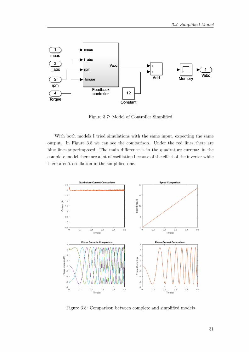
Figure 3.7: Model of Controller Simplified
With both models I tried simulations with the same input, expecting the sameoutput. In Figure 3.8 we can see the comparison. Under the red lines there areblue lines superimposed. The main difference is in the quadrature current: in thecomplete model there are a lot of oscillation because of the effect of the inverter whilethere aren’t oscillation in the simplified one.
Figure 3.8: Comparison between complete and simplified models
31
3. Field Oriented Control Model
3.3 Validation of the Model
To validate the model tests in various condition was made with the real motorand then on simulation.
1. Current Control
(a) Step Response - Current with motor Blocked
(b) Step Response - Speed Variaton
(c) Regime Current
2. Speed Control
(a) Step Response - Speed Variation
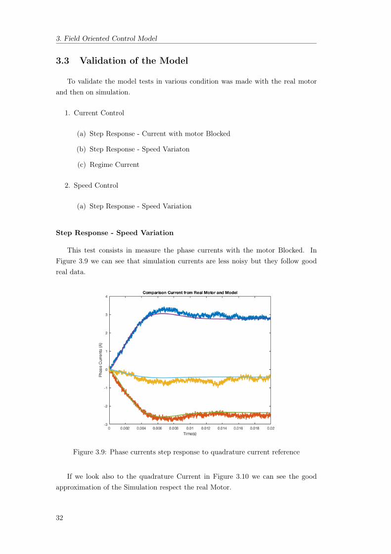
Step Response - Speed Variation
This test consists in measure the phase currents with the motor Blocked. InFigure 3.9 we can see that simulation currents are less noisy but they follow goodreal data.
Figure 3.9: Phase currents step response to quadrature current reference
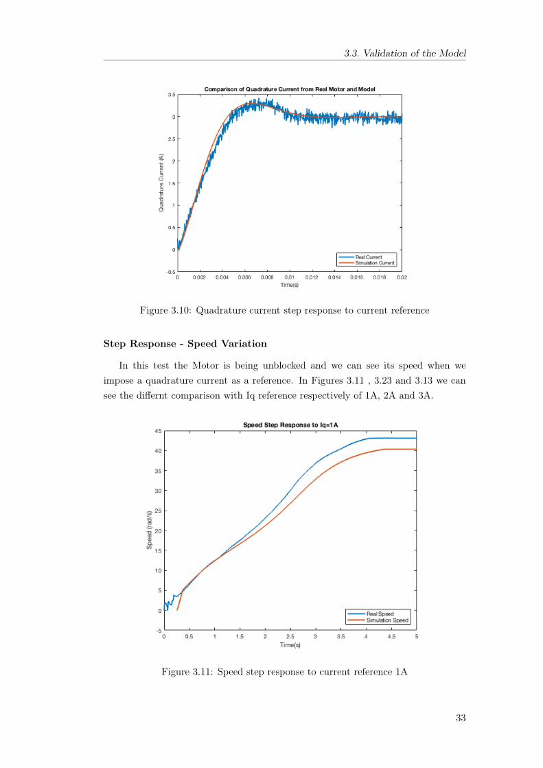
If we look also to the quadrature Current in Figure 3.10 we can see the goodapproximation of the Simulation respect the real Motor.
32
3.3. Validation of the Model
Figure 3.10: Quadrature current step response to current reference
Step Response - Speed Variation
In this test the Motor is being unblocked and we can see its speed when weimpose a quadrature current as a reference. In Figures 3.11 , 3.23 and 3.13 we cansee the differnt comparison with Iq reference respectively of 1A, 2A and 3A.
Figure 3.11: Speed step response to current reference 1A
33
3. Field Oriented Control Model
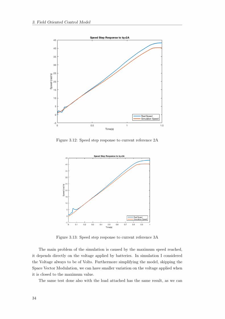
Figure 3.12: Speed step response to current reference 2A
Figure 3.13: Speed step response to current reference 3A
The main problem of the simulation is caused by the maximum speed reached,it depends directly on the voltage applied by batteries. In simulation I consideredthe Voltage always to be of Volts. Furthermore simplifying the model, skipping theSpace Vector Modulation, we can have smaller variation on the voltage applied whenit is closed to the maximum value.
The same test done also with the load attached has the same result, as we can
34
3.3. Validation of the Model
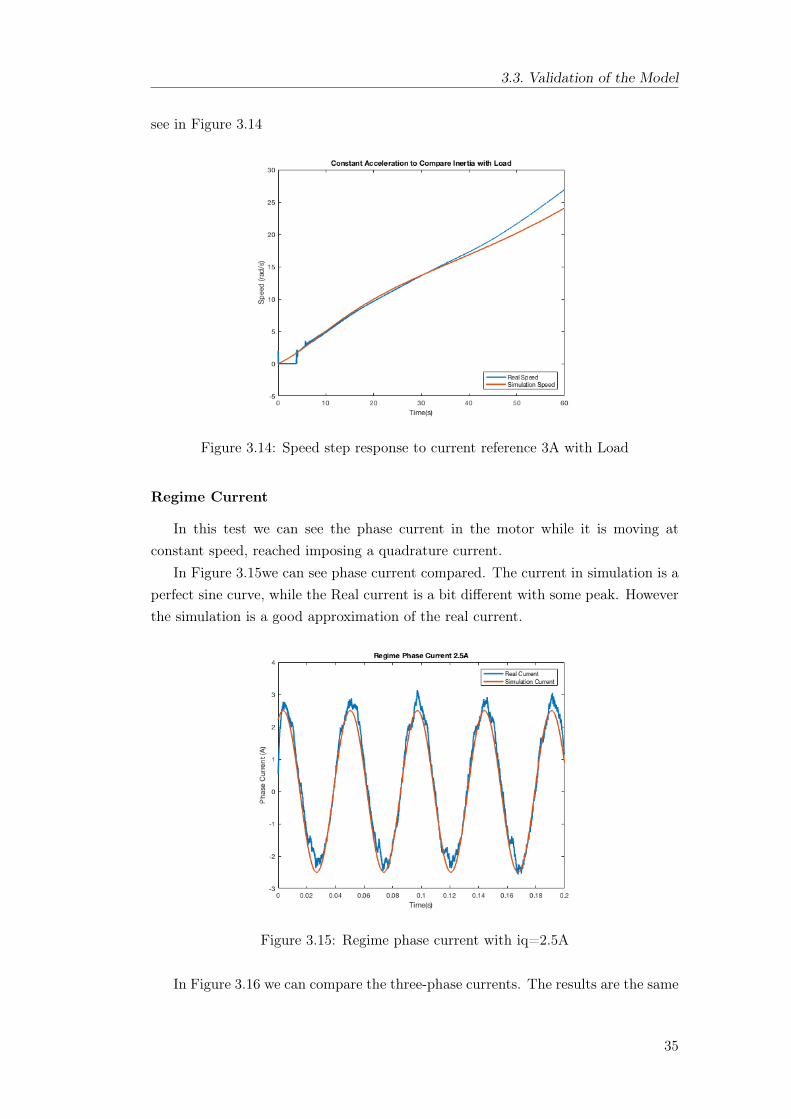
see in Figure 3.14
Figure 3.14: Speed step response to current reference 3A with Load
Regime Current
In this test we can see the phase current in the motor while it is moving atconstant speed, reached imposing a quadrature current.
In Figure 3.15we can see phase current compared. The current in simulation is aperfect sine curve, while the Real current is a bit different with some peak. Howeverthe simulation is a good approximation of the real current.
Figure 3.15: Regime phase current with iq=2.5A
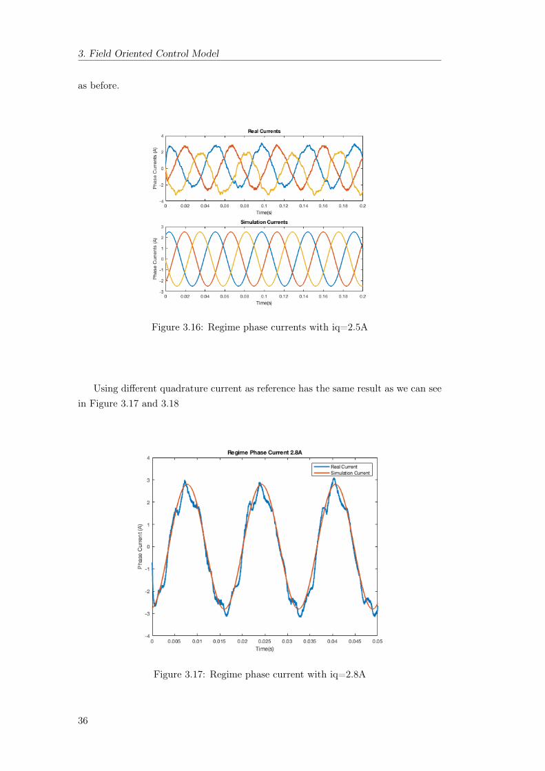
In Figure 3.16 we can compare the three-phase currents. The results are the same
35
3. Field Oriented Control Model
as before.
Figure 3.16: Regime phase currents with iq=2.5A
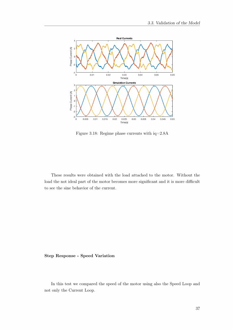
Using different quadrature current as reference has the same result as we can seein Figure 3.17 and 3.18
Figure 3.17: Regime phase current with iq=2.8A
36
3.3. Validation of the Model
Figure 3.18: Regime phase currents with iq=2.8A
These results were obtained with the load attached to the motor. Without theload the not ideal part of the motor becomes more significant and it is more difficultto see the sine behavior of the current.
Step Response - Speed Variation
In this test we compared the speed of the motor using also the Speed Loop andnot only the Current Loop.
37
3. Field Oriented Control Model
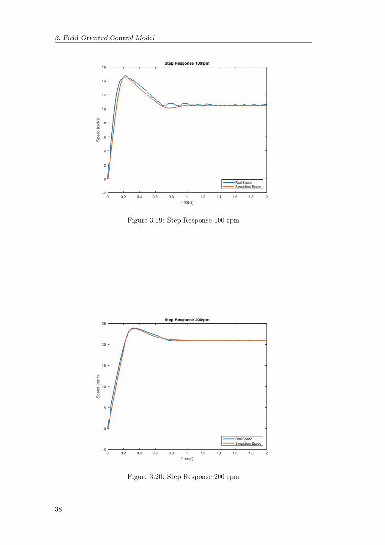
Figure 3.19: Step Response 100 rpm
Figure 3.20: Step Response 200 rpm
38
3.4. Controller Parameters
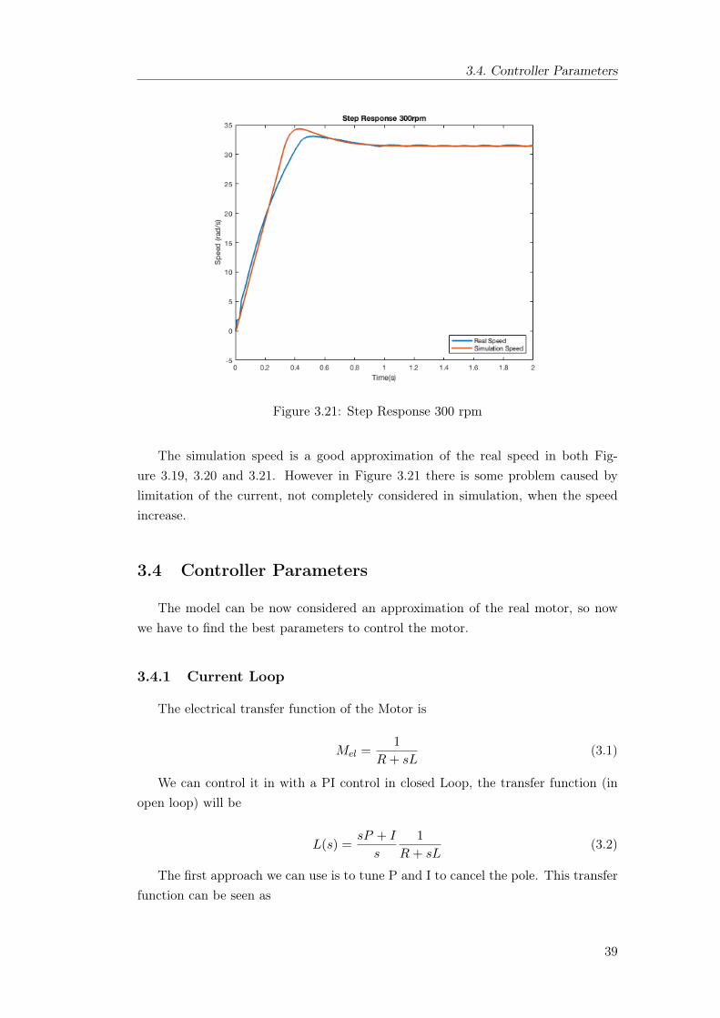
Figure 3.21: Step Response 300 rpm
The simulation speed is a good approximation of the real speed in both Fig-ure 3.19, 3.20 and 3.21. However in Figure 3.21 there is some problem caused bylimitation of the current, not completely considered in simulation, when the speedincrease.
3.4 Controller Parameters
The model can be now considered an approximation of the real motor, so nowwe have to find the best parameters to control the motor.
3.4.1 Current Loop
The electrical transfer function of the Motor is
Mel =1
R+ sL(3.1)
We can control it in with a PI control in closed Loop, the transfer function (inopen loop) will be
L(s) =sP + I
s
1
R+ sL(3.2)
The first approach we can use is to tune P and I to cancel the pole. This transferfunction can be seen as
39
3. Field Oriented Control Model
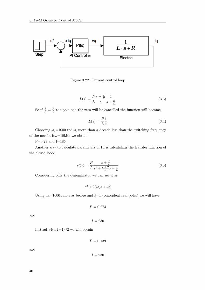
Figure 3.22: Current control loop
L(s) =P
L
s+ IP
s
1
s+ RL
(3.3)
So if IP = R
L the pole and the zero will be cancelled the function will become
L(s) =P
L
1
s(3.4)
Choosing ω0=1000 rad/s, more than a decade less than the switching frequencyof the mosfet fsw=10kHz we obtain
P=0.23 and I=186Another way to calculate parameters of PI is calculating the transfer function of
the closed loop:
F (s) =P
L
s+ IP
s2 + P+RL s+ I
L
(3.5)
Considering only the denominator we can see it as
s2 + 2ξω0s+ ω20
Using ω0=1000 rad/s as before and ξ=1 (coincident real poles) we will have
P = 0.274
andI = 230
Instead with ξ=1/√2 we will obtain
P = 0.139
andI = 230
40
3.4. Controller Parameters
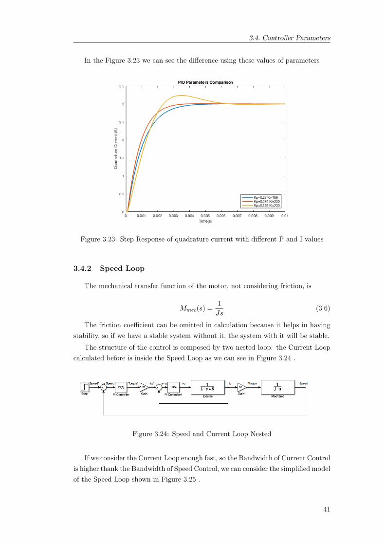
In the Figure 3.23 we can see the difference using these values of parameters
Figure 3.23: Step Response of quadrature current with different P and I values
3.4.2 Speed Loop
The mechanical transfer function of the motor, not considering friction, is
Mmec(s) =1
Js(3.6)
The friction coefficient can be omitted in calculation because it helps in havingstability, so if we have a stable system without it, the system with it will be stable.
The structure of the control is composed by two nested loop: the Current Loopcalculated before is inside the Speed Loop as we can see in Figure 3.24 .
Figure 3.24: Speed and Current Loop Nested
If we consider the Current Loop enough fast, so the Bandwidth of Current Controlis higher thank the Bandwidth of Speed Control, we can consider the simplified modelof the Speed Loop shown in Figure 3.25 .
41
3. Field Oriented Control Model
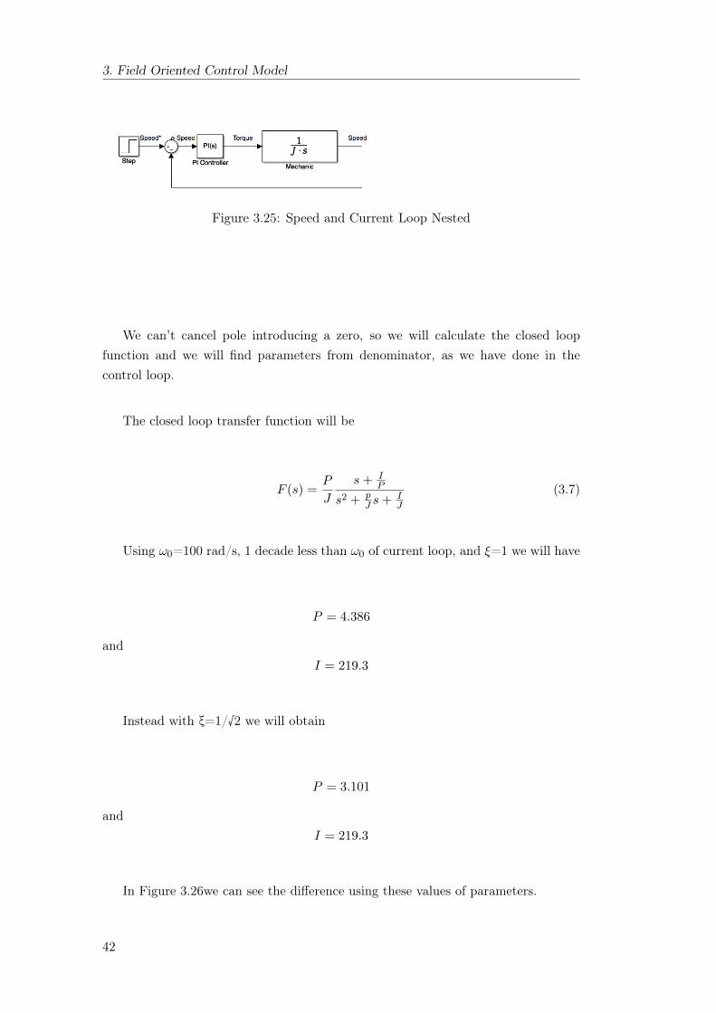
Figure 3.25: Speed and Current Loop Nested
We can’t cancel pole introducing a zero, so we will calculate the closed loopfunction and we will find parameters from denominator, as we have done in thecontrol loop.
The closed loop transfer function will be
F (s) =P
J
s+ IP
s2 + pJ s+ I
J
(3.7)
Using ω0=100 rad/s, 1 decade less than ω0 of current loop, and ξ=1 we will have
P = 4.386
andI = 219.3
Instead with ξ=1/√2 we will obtain
P = 3.101
andI = 219.3
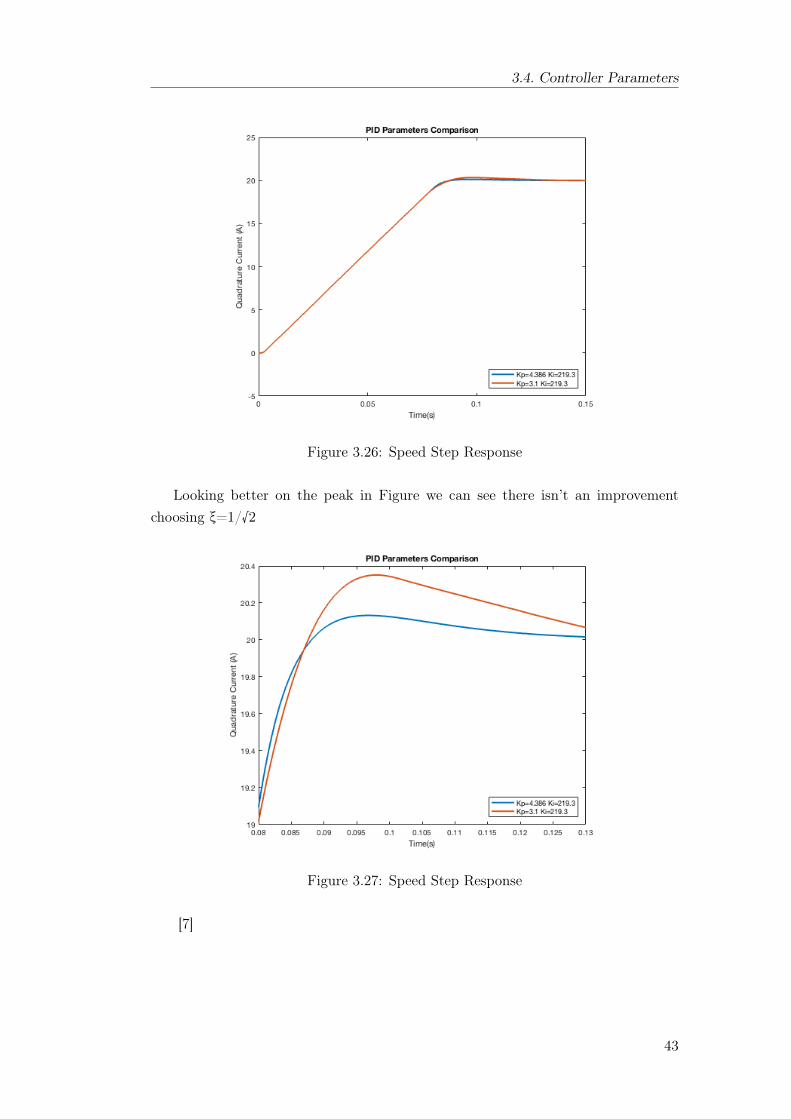
In Figure 3.26we can see the difference using these values of parameters.
42
3.4. Controller Parameters
Figure 3.26: Speed Step Response
Looking better on the peak in Figure we can see there isn’t an improvementchoosing ξ=1/√2
Figure 3.27: Speed Step Response
[7]
43

3. Field Oriented Control Model
44
Chapter 4
Brushless DC Control Model
4.1 Simulink Model
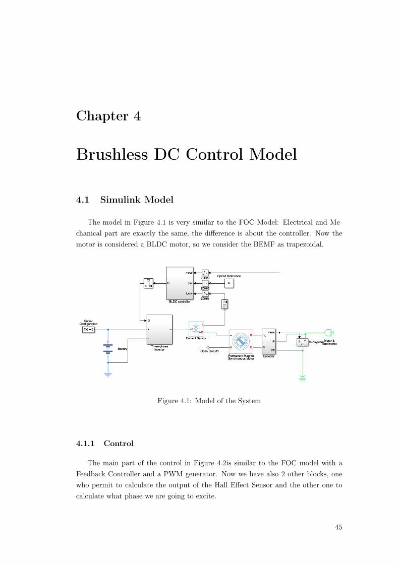
The model in Figure 4.1 is very similar to the FOC Model: Electrical and Me-chanical part are exactly the same, the difference is about the controller. Now themotor is considered a BLDC motor, so we consider the BEMF as trapezoidal.
Figure 4.1: Model of the System
4.1.1 Control
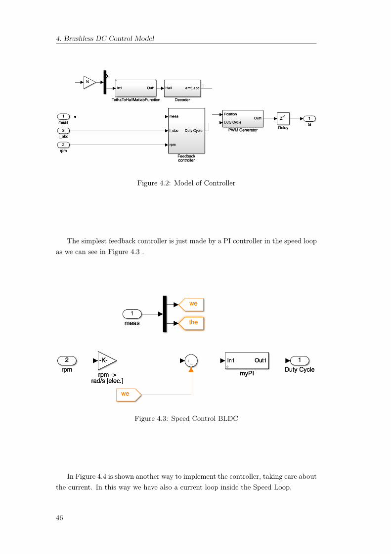
The main part of the control in Figure 4.2is similar to the FOC model with aFeedback Controller and a PWM generator. Now we have also 2 other blocks, onewho permit to calculate the output of the Hall Effect Sensor and the other one tocalculate what phase we are going to excite.
45
4. Brushless DC Control Model
Figure 4.2: Model of Controller
The simplest feedback controller is just made by a PI controller in the speed loopas we can see in Figure 4.3 .
Figure 4.3: Speed Control BLDC
In Figure 4.4 is shown another way to implement the controller, taking care aboutthe current. In this way we have also a current loop inside the Speed Loop.
46
4.2. Simplified Model
Figure 4.4: Speed Control BLDC with Current Loop
4.2 Simplified Model
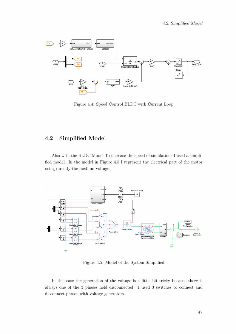
Also with the BLDC Model To increase the speed of simulations I used a simpli-fied model. In the model in Figure 4.5 I represent the electrical part of the motorusing directly the medium voltage.
Figure 4.5: Model of the System Simplified
In this case the generation of the voltage is a little bit tricky because there isalways one of the 3 phases held disconnected. I used 3 switches to connect anddisconnect phases with voltage generators.
47
4. Brushless DC Control Model
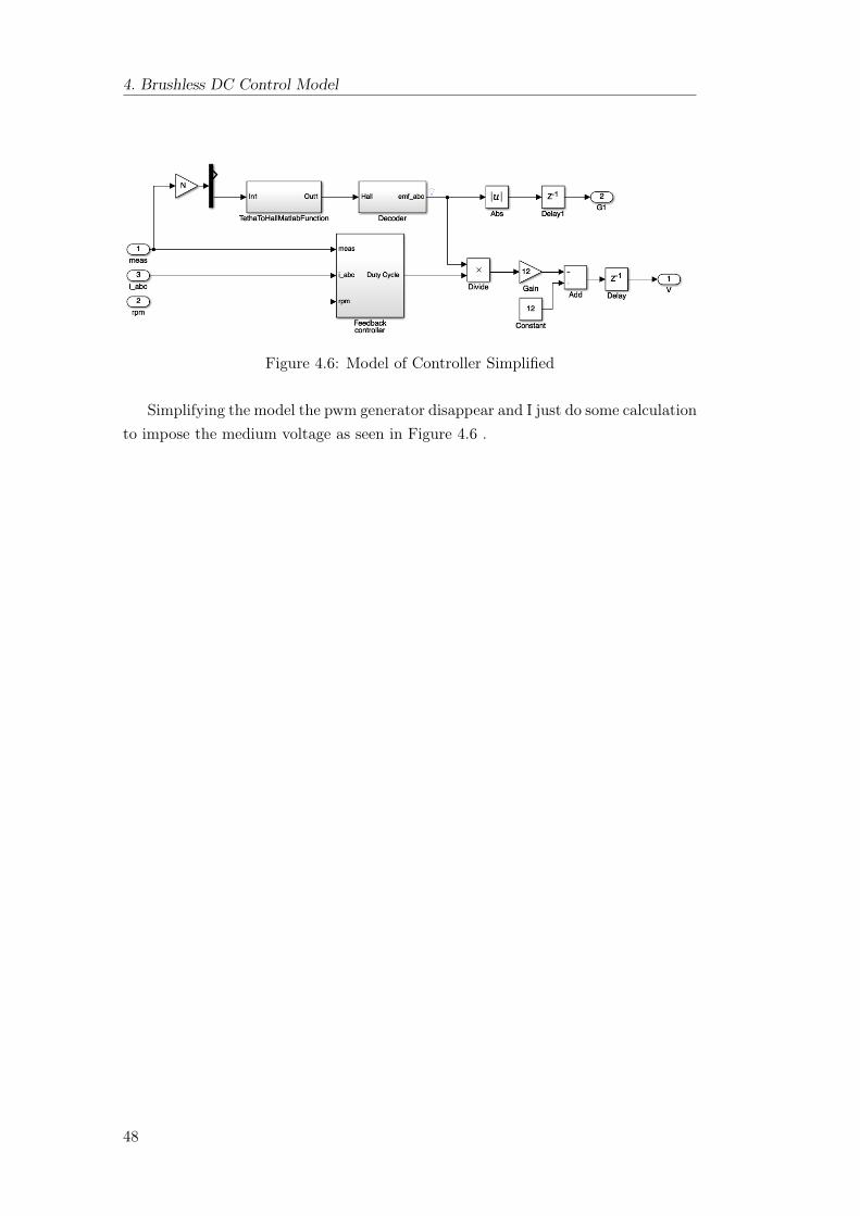
Figure 4.6: Model of Controller Simplified
Simplifying the model the pwm generator disappear and I just do some calculationto impose the medium voltage as seen in Figure 4.6 .
48
4.3. Validation of the Model
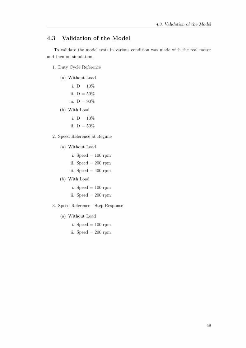
4.3 Validation of the Model
To validate the model tests in various condition was made with the real motorand then on simulation.
1. Duty Cycle Reference
(a) Without Load
i. D = 10%
ii. D = 50%
iii. D = 90%
(b) With Load
i. D = 10%
ii. D = 50%
2. Speed Reference at Regime
(a) Without Load
i. Speed = 100 rpm
ii. Speed = 200 rpm
iii. Speed = 400 rpm
(b) With Load
i. Speed = 100 rpm
ii. Speed = 200 rpm
3. Speed Reference - Step Response
(a) Without Load
i. Speed = 100 rpm
ii. Speed = 200 rpm
49
4. Brushless DC Control Model
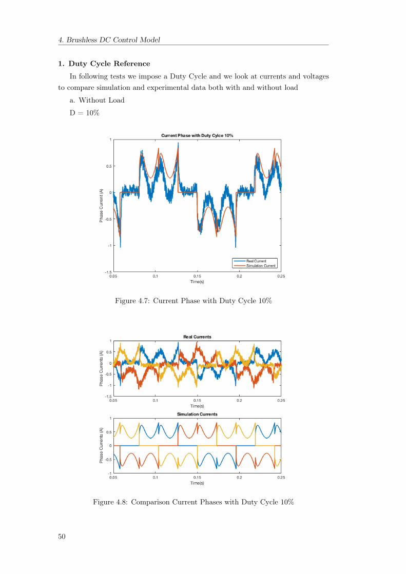
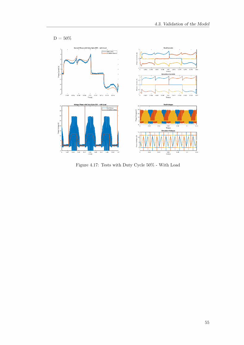
1. Duty Cycle Reference
In following tests we impose a Duty Cycle and we look at currents and voltagesto compare simulation and experimental data both with and without load
a. Without Load
D = 10%
Figure 4.7: Current Phase with Duty Cycle 10%
Figure 4.8: Comparison Current Phases with Duty Cycle 10%
50
4.3. Validation of the Model
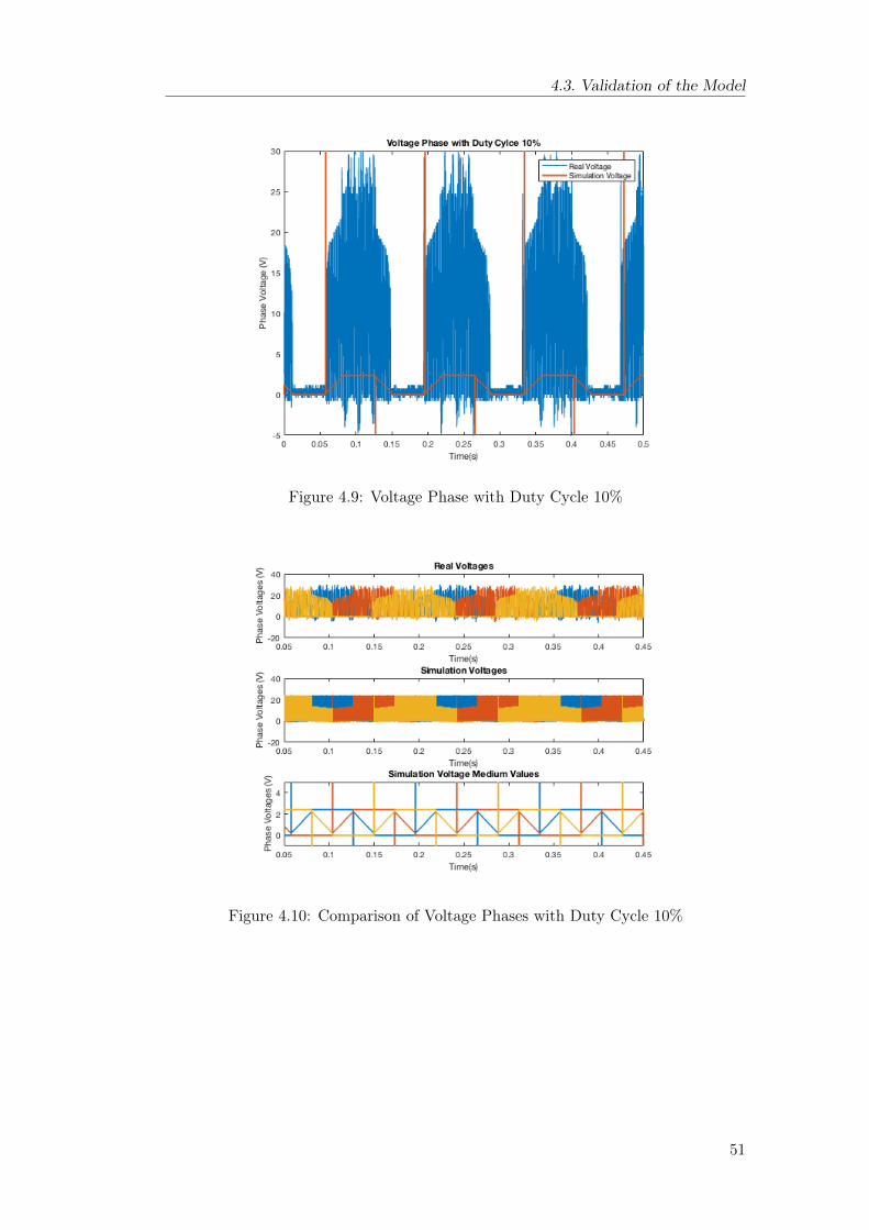
Figure 4.9: Voltage Phase with Duty Cycle 10%
Figure 4.10: Comparison of Voltage Phases with Duty Cycle 10%
51
4. Brushless DC Control Model
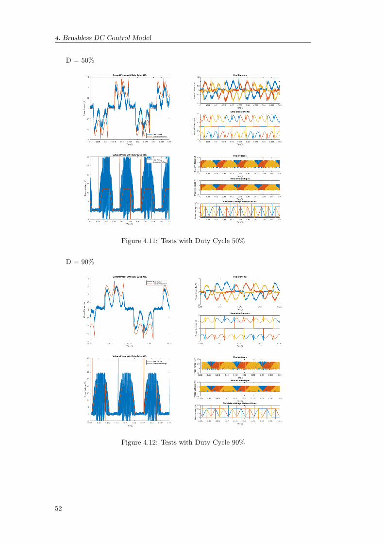
D = 50%
Figure 4.11: Tests with Duty Cycle 50%
D = 90%
Figure 4.12: Tests with Duty Cycle 90%
52
4.3. Validation of the Model
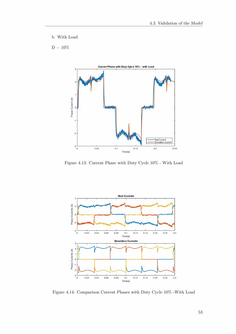
b. With Load
D = 10%
Figure 4.13: Current Phase with Duty Cycle 10% - With Load
Figure 4.14: Comparison Current Phases with Duty Cycle 10% -With Load
53
4. Brushless DC Control Model
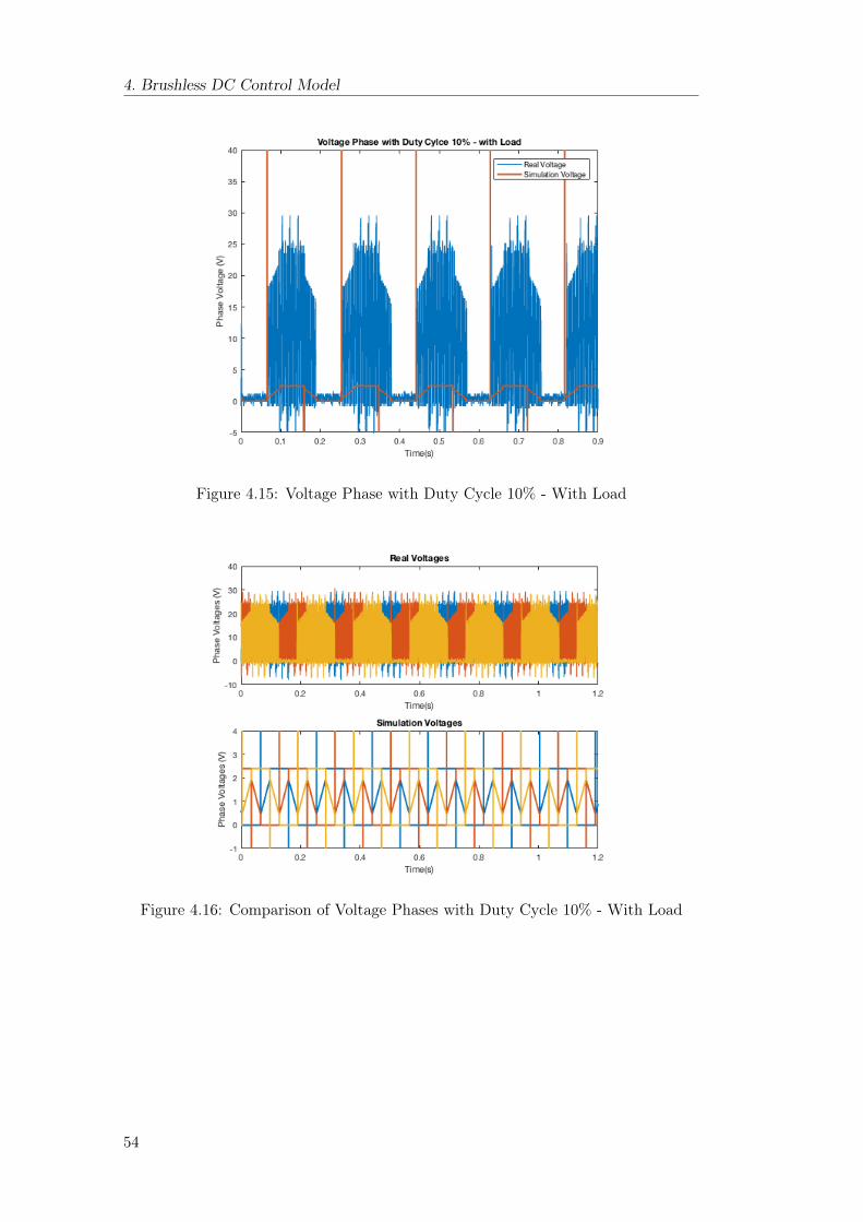
Figure 4.15: Voltage Phase with Duty Cycle 10% - With Load
Figure 4.16: Comparison of Voltage Phases with Duty Cycle 10% - With Load
54
4.3. Validation of the Model
D = 50%
Figure 4.17: Tests with Duty Cycle 50% - With Load
55
4. Brushless DC Control Model
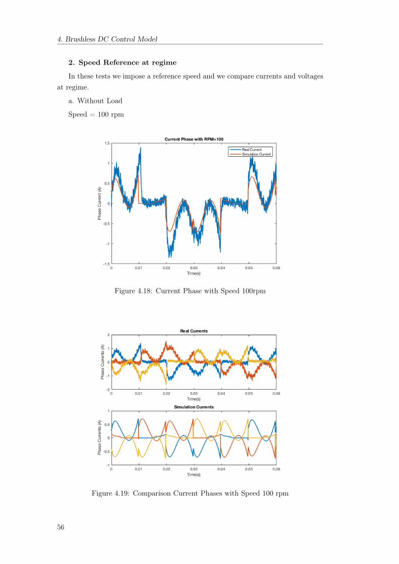
2. Speed Reference at regime
In these tests we impose a reference speed and we compare currents and voltagesat regime.
a. Without Load
Speed = 100 rpm
Figure 4.18: Current Phase with Speed 100rpm
Figure 4.19: Comparison Current Phases with Speed 100 rpm
56
4.3. Validation of the Model
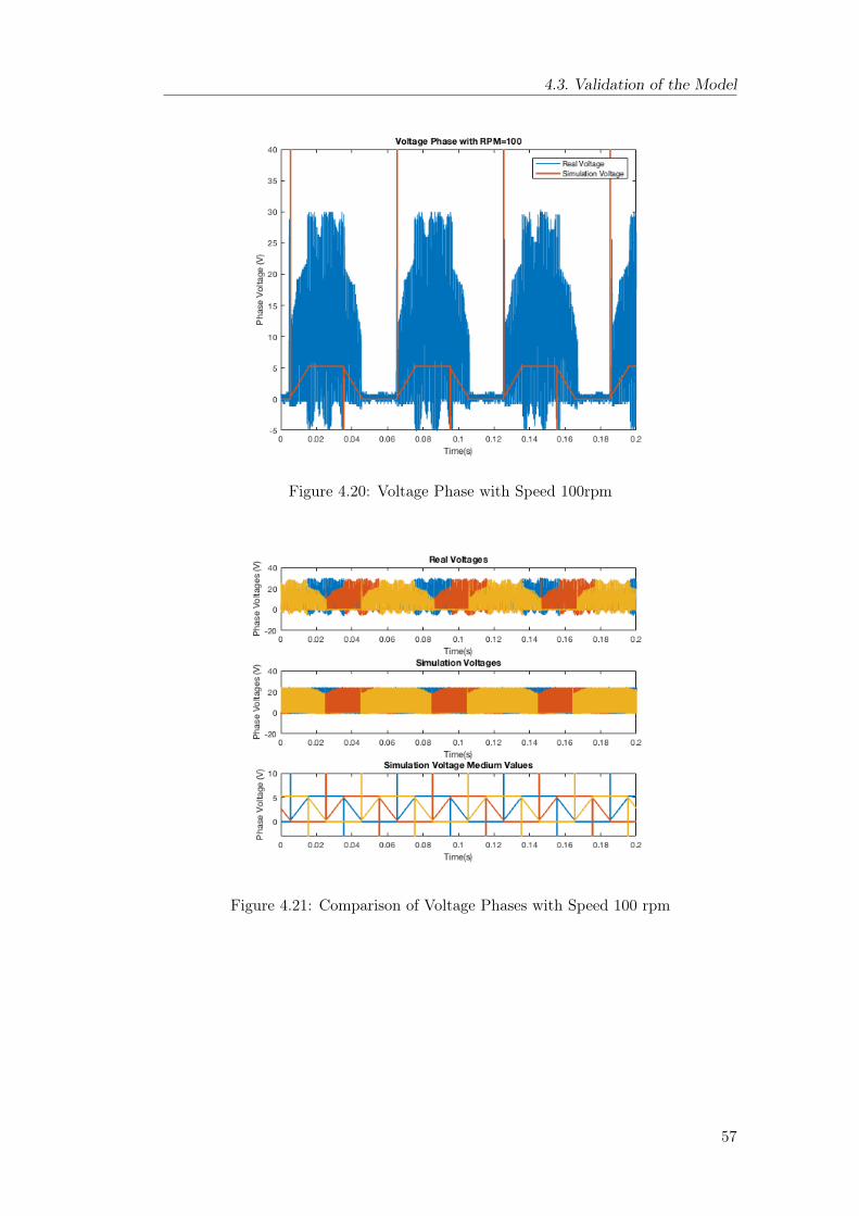
Figure 4.20: Voltage Phase with Speed 100rpm
Figure 4.21: Comparison of Voltage Phases with Speed 100 rpm
57
4. Brushless DC Control Model
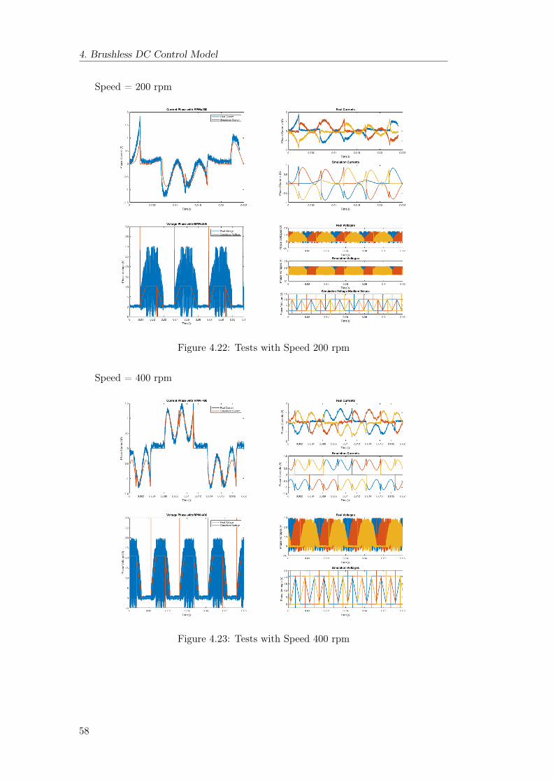
Speed = 200 rpm
Figure 4.22: Tests with Speed 200 rpm
Speed = 400 rpm
Figure 4.23: Tests with Speed 400 rpm
58
4.3. Validation of the Model
b.With Load
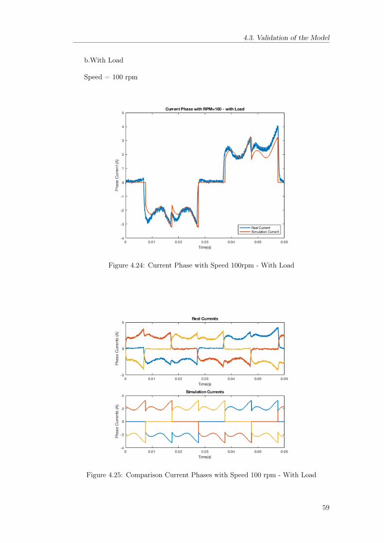
Speed = 100 rpm
Figure 4.24: Current Phase with Speed 100rpm - With Load
Figure 4.25: Comparison Current Phases with Speed 100 rpm - With Load
59
4. Brushless DC Control Model
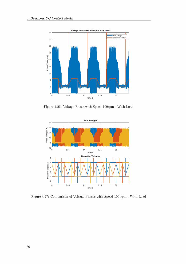
Figure 4.26: Voltage Phase with Speed 100rpm - With Load
Figure 4.27: Comparison of Voltage Phases with Speed 100 rpm - With Load
60
4.3. Validation of the Model
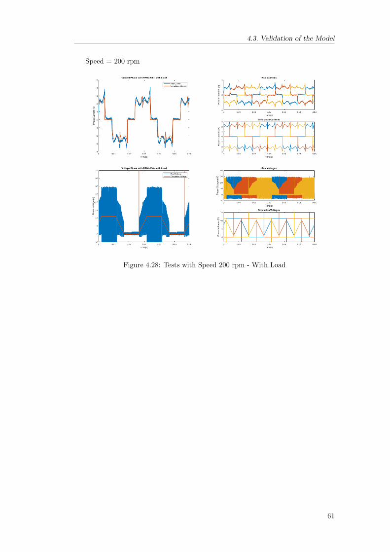
Speed = 200 rpm
Figure 4.28: Tests with Speed 200 rpm - With Load
61
4. Brushless DC Control Model
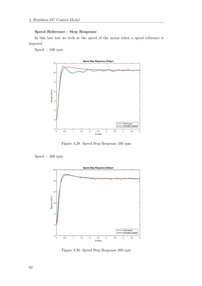
Speed Reference - Step Response
In this last test we look at the speed of the motor when a speed reference isimposed
Speed = 100 rpm
Figure 4.29: Speed Step Response 100 rpm
Speed = 200 rpm
Figure 4.30: Speed Step Response 200 rpm
62
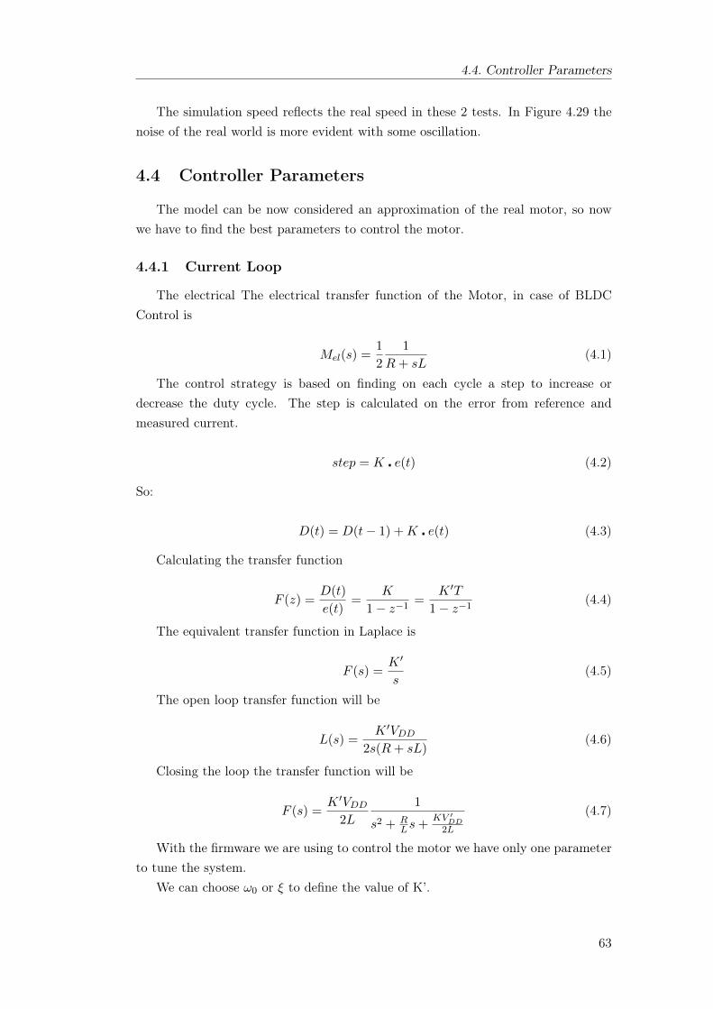
4.4. Controller Parameters
The simulation speed reflects the real speed in these 2 tests. In Figure 4.29 thenoise of the real world is more evident with some oscillation.
4.4 Controller Parameters
The model can be now considered an approximation of the real motor, so nowwe have to find the best parameters to control the motor.
4.4.1 Current Loop
The electrical The electrical transfer function of the Motor, in case of BLDCControl is
Mel(s) =1
2
1
R+ sL(4.1)
The control strategy is based on finding on each cycle a step to increase ordecrease the duty cycle. The step is calculated on the error from reference andmeasured current.
step = K e(t) (4.2)
So:
D(t) = D(t− 1) +K e(t) (4.3)
Calculating the transfer function
F (z) =D(t)
e(t)=
K
1− z−1=
K ′T
1− z−1(4.4)
The equivalent transfer function in Laplace is
F (s) =K ′
s(4.5)
The open loop transfer function will be
L(s) =K ′VDD
2s(R+ sL)(4.6)
Closing the loop the transfer function will be
F (s) =K ′VDD
2L
1
s2 + RLs+
KV ′DD
2L
(4.7)
With the firmware we are using to control the motor we have only one parameterto tune the system.
We can choose ω0 or ξ to define the value of K’.
63
4. Brushless DC Control Model
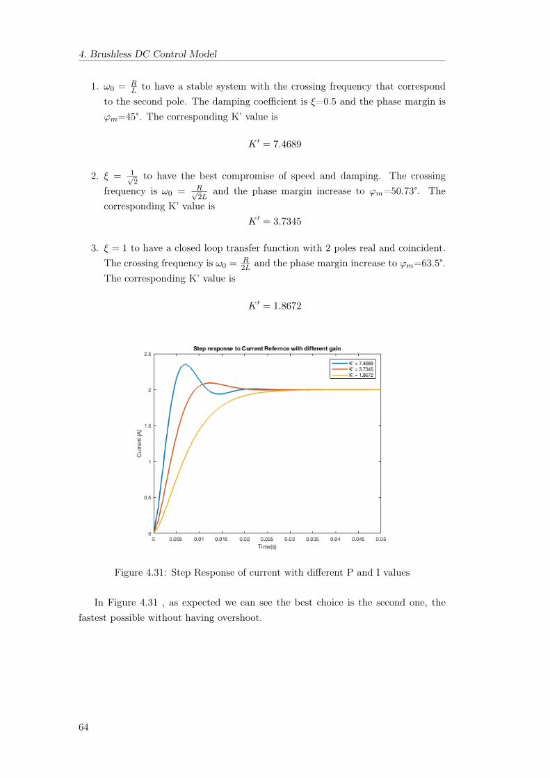
1. ω0 = RL to have a stable system with the crossing frequency that correspond
to the second pole. The damping coefficient is ξ=0.5 and the phase margin isϕm=45°. The corresponding K’ value is
K ′ = 7.4689
2. ξ = 1√2to have the best compromise of speed and damping. The crossing
frequency is ω0 = R√2L
and the phase margin increase to ϕm=50.73°. Thecorresponding K’ value is
K ′ = 3.7345
3. ξ = 1 to have a closed loop transfer function with 2 poles real and coincident.The crossing frequency is ω0 = R
2L and the phase margin increase to ϕm=63.5°.The corresponding K’ value is
K ′ = 1.8672
Figure 4.31: Step Response of current with different P and I values
In Figure 4.31 , as expected we can see the best choice is the second one, thefastest possible without having overshoot.
64
4.4. Controller Parameters
4.4.2 Speed Loop
Not depending on the control strategy, the mechanical transfer function of themotor is the same seen before in the FOC control chapter. We can still not considerthe friction that help stability
Mmec(s) =1
Js(4.8)
We use a PI Controller as in FOC Control and we will have the same transferfunction in closed loop
F (s) =P
J
s+ IP
s2 + pJ s+ I
J
(4.9)
Calculation are the same as before, but we have to consider we have a lower ω0
depending on a lower crossing frequency in the Current Loop on Trapezoidal Control.
Using ω0=34 rad/s, 1 decade less than ω0 of current loop, and ξ = 1√2we will
have
P = 1.4893
andI = 25.3164
Instead with ξ = 1 we will obtain
P = 0.7747
andI = 25.3164
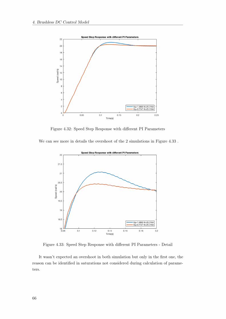
In Figure 4.32 we can compare the step response of the speed in these 2 cases.
65
4. Brushless DC Control Model
Figure 4.32: Speed Step Response with different PI Parameters
We can see more in details the overshoot of the 2 simulations in Figure 4.33 .
Figure 4.33: Speed Step Response with different PI Parameters - Detail
It wasn’t expected an overshoot in both simulation but only in the first one, thereason can be identified in saturations not considered during calculation of parame-ters.
66
Chapter 5
Comparison between FOC and6-Step
In this last chapter we are going to compare results obtained in the previous 2chapters. We are going to ask ourselves which one is the better control strategy.
5.1 Speed Step Response Comparison
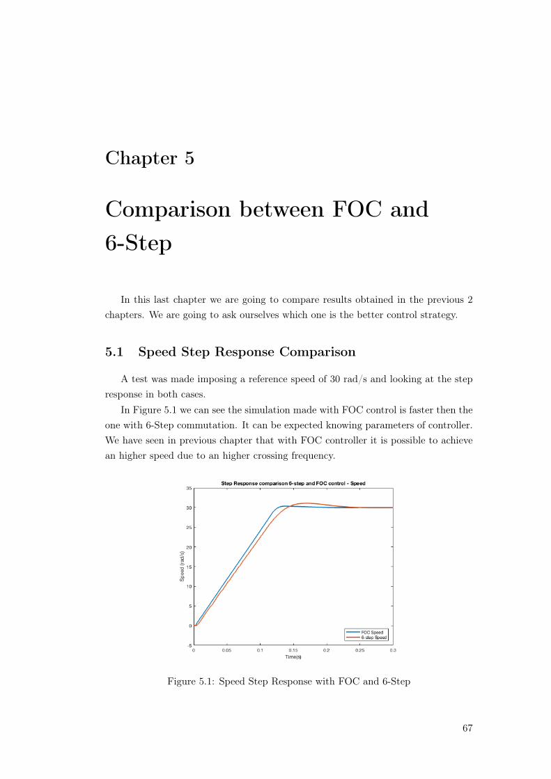
A test was made imposing a reference speed of 30 rad/s and looking at the stepresponse in both cases.
In Figure 5.1 we can see the simulation made with FOC control is faster then theone with 6-Step commutation. It can be expected knowing parameters of controller.We have seen in previous chapter that with FOC controller it is possible to achievean higher speed due to an higher crossing frequency.
Figure 5.1: Speed Step Response with FOC and 6-Step
67
5. Comparison between FOC and 6-Step
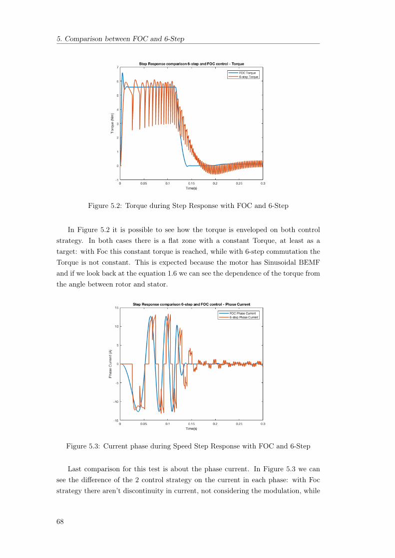
Figure 5.2: Torque during Step Response with FOC and 6-Step
In Figure 5.2 it is possible to see how the torque is enveloped on both controlstrategy. In both cases there is a flat zone with a constant Torque, at least as atarget: with Foc this constant torque is reached, while with 6-step commutation theTorque is not constant. This is expected because the motor has Sinusoidal BEMFand if we look back at the equation 1.6 we can see the dependence of the torque fromthe angle between rotor and stator.
Figure 5.3: Current phase during Speed Step Response with FOC and 6-Step
Last comparison for this test is about the phase current. In Figure 5.3 we cansee the difference of the 2 control strategy on the current in each phase: with Focstrategy there aren’t discontinuity in current, not considering the modulation, while
68
5.2. Comparison at Regime
using 6 step commutation it is possible to see the current going to zero alternatively.It is interesting see the shape of both control method is at the first order the same,without considering the lag increasing in 6-step due to a lower speed as we have seenin Figure 5.1 .
5.2 Comparison at Regime
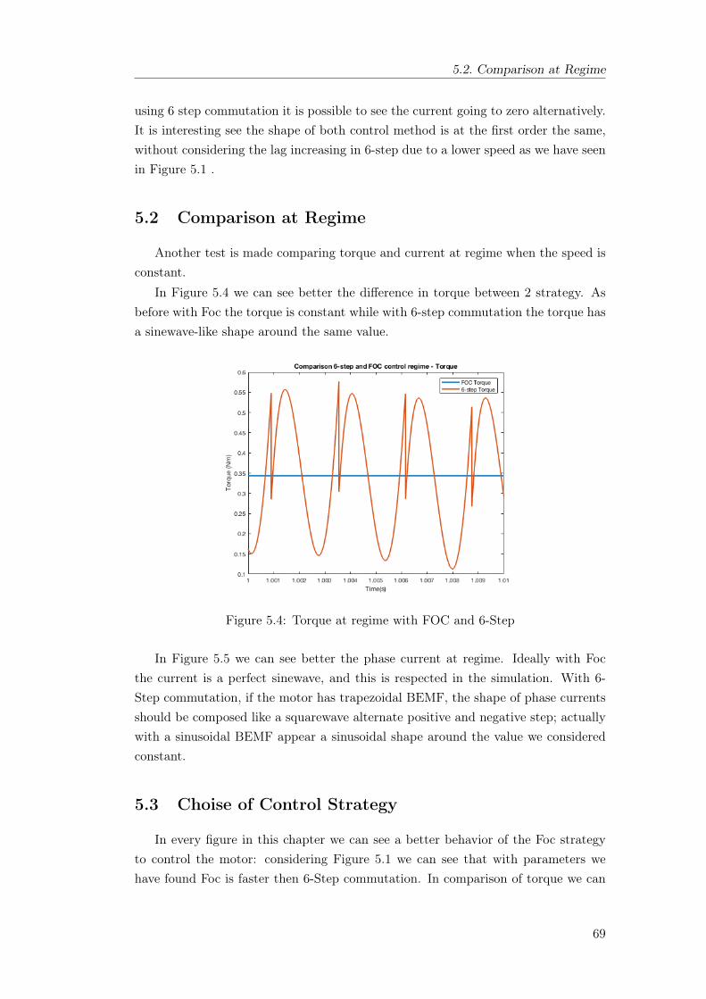
Another test is made comparing torque and current at regime when the speed isconstant.
In Figure 5.4 we can see better the difference in torque between 2 strategy. Asbefore with Foc the torque is constant while with 6-step commutation the torque hasa sinewave-like shape around the same value.
Figure 5.4: Torque at regime with FOC and 6-Step
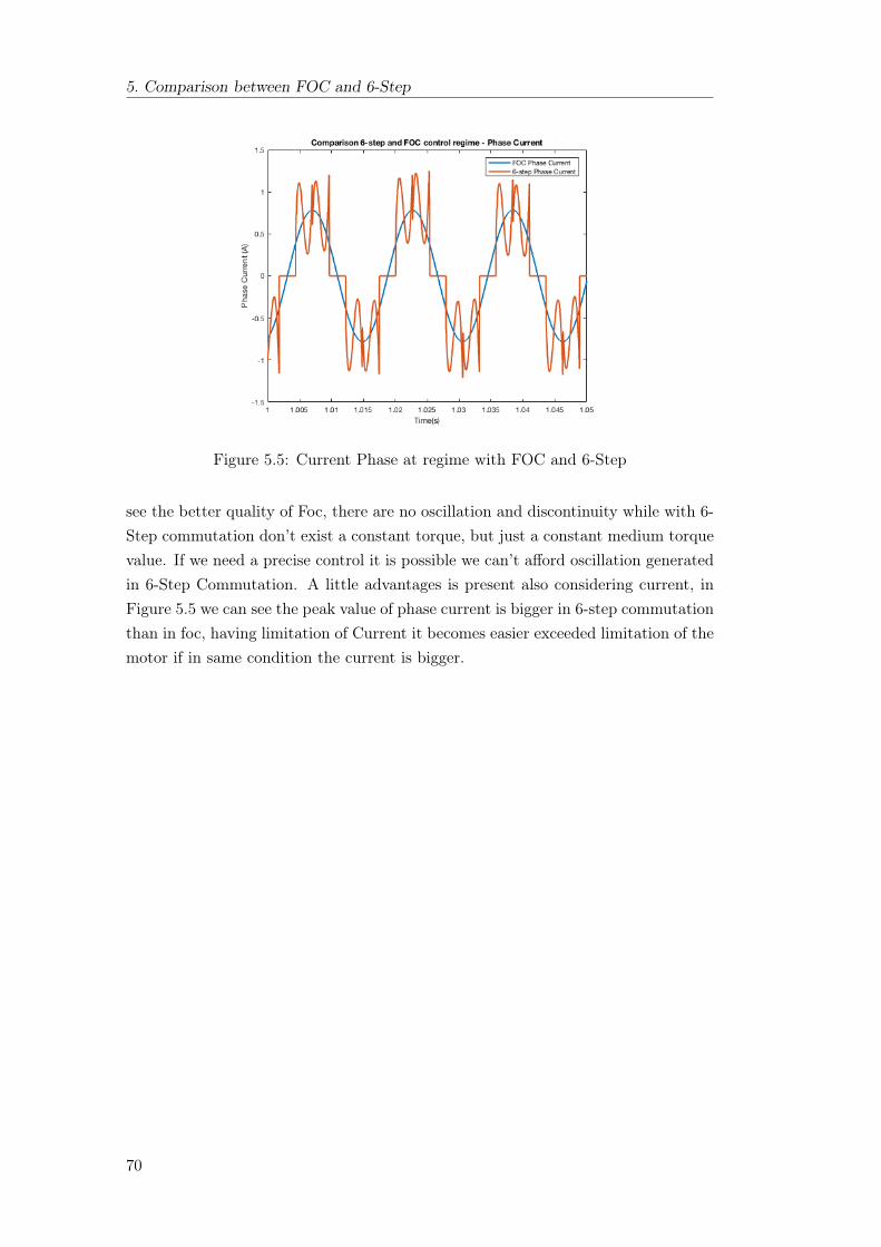
In Figure 5.5 we can see better the phase current at regime. Ideally with Focthe current is a perfect sinewave, and this is respected in the simulation. With 6-Step commutation, if the motor has trapezoidal BEMF, the shape of phase currentsshould be composed like a squarewave alternate positive and negative step; actuallywith a sinusoidal BEMF appear a sinusoidal shape around the value we consideredconstant.
5.3 Choise of Control Strategy
In every figure in this chapter we can see a better behavior of the Foc strategyto control the motor: considering Figure 5.1 we can see that with parameters wehave found Foc is faster then 6-Step commutation. In comparison of torque we can
69
5. Comparison between FOC and 6-Step
Figure 5.5: Current Phase at regime with FOC and 6-Step
see the better quality of Foc, there are no oscillation and discontinuity while with 6-Step commutation don’t exist a constant torque, but just a constant medium torquevalue. If we need a precise control it is possible we can’t afford oscillation generatedin 6-Step Commutation. A little advantages is present also considering current, inFigure 5.5 we can see the peak value of phase current is bigger in 6-step commutationthan in foc, having limitation of Current it becomes easier exceeded limitation of themotor if in same condition the current is bigger.
70
Conclusions
The purpose of this thesis was to realize a Simulink model of the in-Wheel brush-less motor and its control strategy.
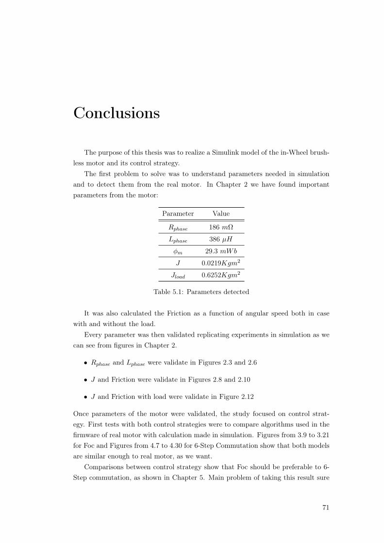
The first problem to solve was to understand parameters needed in simulationand to detect them from the real motor. In Chapter 2 we have found importantparameters from the motor:
Parameter Value
Rphase 186 mΩ
Lphase 386 µH
φm 29.3 mWb
J 0.0219Kgm2
Jload 0.6252Kgm2
Table 5.1: Parameters detected
It was also calculated the Friction as a function of angular speed both in casewith and without the load.
Every parameter was then validated replicating experiments in simulation as wecan see from figures in Chapter 2.
• Rphase and Lphase were validate in Figures 2.3 and 2.6
• J and Friction were validate in Figures 2.8 and 2.10
• J and Friction with load were validate in Figure 2.12
Once parameters of the motor were validated, the study focused on control strat-egy. First tests with both control strategies were to compare algorithms used in thefirmware of real motor with calculation made in simulation. Figures from 3.9 to 3.21for Foc and Figures from 4.7 to 4.30 for 6-Step Commutation show that both modelsare similar enough to real motor, as we want.
Comparisons between control strategy show that Foc should be preferable to 6-Step commutation, as shown in Chapter 5. Main problem of taking this result sure
71
Conclusions
is represented by the real world, in simulation we consider every sensor ideal: thereis no noise and there isn’t any delay. The real motor still have some future notconsidered:
1. Only two currents can be read through 2 shunt resistors. These resistors aren’ton the phase but they are on the leg of the inverter. From these currents it ishowever possible to reconstruct phase current, but it can become problematicdue to the fact we need the current flow at least one moment to ground to readits value.
2. Inverter was simplified due to long time of simulation. Too low switching fre-quency of the invert can make the system instable. Calculation of parametersof Controller should be done taking care of this frequency: considering a cross-ing frequency enough lower then switching frequency every problem should beavoided.
3. Angular position is read only with hall effect sensors. With 6-step commutationthis isn’t a problem, we divide the angle in 6 sectors exactly as hall effect sensorsdo. With Foc technic not having a perfect position can be problematic becauseit is needed in Park transformation.
Improvements regarding the model can be done in these 3 directions.
72
Bibliography
[1] DC AN885-Brushless. Motor fundamentals. Microchip Technology Inc, 2003.
[2] Nahas Basheer. Introduction to electric motors.(https://mediatoget.blogspot.it/2012/01/introduction-to-electric-motors.html).
[3] Benjamin. Vesc firmware. (https://www.vesc-project.com/node/309).
[4] Edison Tech Center. The electric motor.(http://www.edisontechcenter.org/electricmotors.html).
[5] Marco Baur Luca Bascetta and Giambattista Gruosso. Robi: A prototype mobilemanipulator for agricultural applications. electronics, 2017.
[6] Gianantonio Magnani, Gianni Ferretti, and Paolo Rocco. Tecnologie dei sistemidi controllo. Mc-Graw-Hill libri Italia, 2000.
[7] Nicola Schiavoni Paolo Bolzern, Riccardo Scattolini. Fondamenti di ControlliAutomatici. McGraw-Hill, 2004.
[8] Hamid A Toliyat and Tilak Gopalarathnam. Ac machines controlled as dc ma-chines (brushless dc machines/electronics). The Power Electronics Handbook,2002.
73

Bibliography
74