Mobile technology: two decades driving economic growth

0

Pag

e0

Mobile technology: two

decades driving economic

growth

Working paper

November 2020

Page | 1

Authors:

Kalvin Bahia Principal Economist, GSMA Intelligence [email protected]

Pau Castells Head of Economic Analysis, GSMA Intelligence [email protected]

Xavier Pedros Senior Economist, GSMA Intelligence [email protected]

mailto:[email protected]



Page | 2

Contents 1. Introduction ........................................................................................................................................... 3

2. Research questions ................................................................................................................................ 5

3. Data ....................................................................................................................................................... 7

4. Empirical strategy .................................................................................................................................. 8

5. Results ................................................................................................................................................. 13

6. Conclusions .......................................................................................................................................... 25

References ............................................................................................................................................... 27

Appendices .............................................................................................................................................. 30

Page | 3

1. Introduction A significant body of empirical research has studied the economic impacts of telecommunications over the last two decades. The impact of fixed communications infrastructure has been covered extensively, mostly looking at technology deployments until 2010.1 Meanwhile, the literature analysing the impacts of mobile technology is more limited, particularly when it comes to the rollout of more recent network technologies. While some studies have considered the rollout of mobile connectivity until 2010, these miss the recent acceleration in the use of mobile broadband through the extension of 3G and 4G.2 Recently, some papers have specifically addressed the impact of mobile broadband globally for the last decade, for example Edquist et al. (2018) and ITU (2018). We contribute to this more recent wave of research in four areas. First, we evaluate the impact of mobile technology from 2000 to 2017 across more than 160 countries – this covers the early deployment of 2G to the 4G cycle, and represents one of the most comprehensive panels in the literature (particularly in the context of the most recent research looking at mobile broadband). Second, while related literature tends to look at the overall impact of mobile technology, we apply a framework to unpick specific impacts of 2G, 3G and 4G technology – addressing the question of whether there are additional impacts with newer infrastructure. Third, we evaluate heterogeneities in the impact of mobile, including network effects from take-up, skills and economic structure – mechanisms that can shift mobile’s impact and that have been largely unexplored globally in recent periods. Finally, using the same panel, this is a novel paper in applying several methods to address endogeneity, including Structural Equations Models (SEM), Dynamic Panel Data (DPD) and Instrumental Variable (IV) approaches – which have been used in the existing literature in different settings. Firstly, we find that mobile technology has significantly driven GDP in the 2000–2017 period – a 10% increase in mobile adoption increased GDP by 0.5% to 1.2%, with these effects remaining broadly stable over the period analysed and materialising over and above fixed infrastructure. Second, we found the subsequent rollout of 2G, 3G and 4G networks has driven increasing impacts. Specifically, mobile’s baseline economic impact increases by about 15% when connections are upgraded to 3G. For connections upgrading from 2G to 4G, the economic impact of mobile increases by approximately 25%.

1 See Bertschek (2017) for a comprehensive literature review. 2 For example, see Thompson & Garbacz 2011, Gruber & Koutroumpis 2011, Aker 2010 or Forero 2013

Page | 4

Third, our analysis for determinants of the impact of mobile reveal important conclusions. We have found that the macroeconomic impacts of mobile increase with adoption, suggesting strong network and learning effects. We also noted countries with more education experience stronger effects, providing evidence of complementarities with human capital accumulation. We also found some evidence of higher impact in economies where services and manufacturing represent a more important part of the economy, further suggesting complementarities with capital and labour in these sectors. The remainder of this paper is organised as follows. Section 2 explains the research questions we explore, framing them in the relevant empirical literature. Following this, Section 3 describes the data and Section 4 details the empirical strategy that we propose for our OLS fixed effects, SEM, IV and DPD frameworks. Section 5 provides results, and Section 6 summarises the key conclusions and implications, in addition to suggesting areas for further research.

Page | 5

2. Research questions

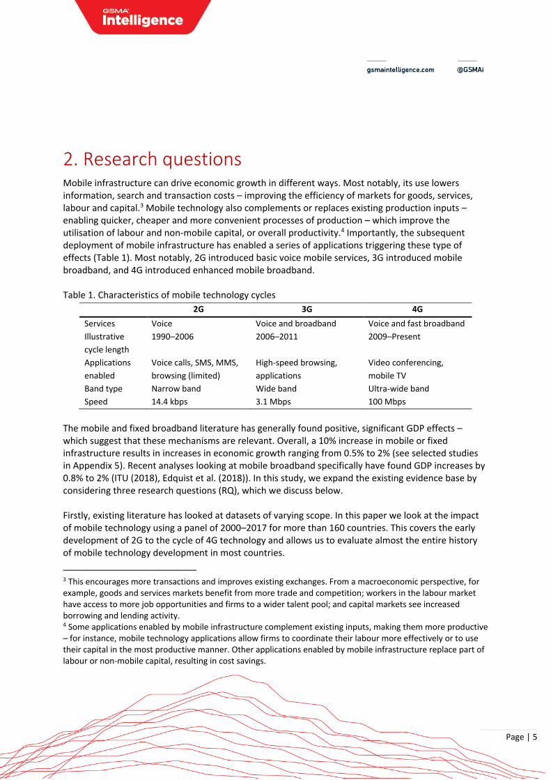
Mobile infrastructure can drive economic growth in different ways. Most notably, its use lowers information, search and transaction costs – improving the efficiency of markets for goods, services, labour and capital.3 Mobile technology also complements or replaces existing production inputs – enabling quicker, cheaper and more convenient processes of production – which improve the utilisation of labour and non-mobile capital, or overall productivity.4 Importantly, the subsequent deployment of mobile infrastructure has enabled a series of applications triggering these type of effects (Table 1). Most notably, 2G introduced basic voice mobile services, 3G introduced mobile broadband, and 4G introduced enhanced mobile broadband. Table 1. Characteristics of mobile technology cycles

2G 3G 4G

Services Voice Voice and broadband Voice and fast broadband

Illustrative

cycle length

1990–2006 2006–2011 2009–Present

Applications

enabled

Voice calls, SMS, MMS,

browsing (limited)

High-speed browsing,

applications

Video conferencing,

mobile TV

Band type Narrow band Wide band Ultra-wide band

Speed 14.4 kbps 3.1 Mbps 100 Mbps

The mobile and fixed broadband literature has generally found positive, significant GDP effects – which suggest that these mechanisms are relevant. Overall, a 10% increase in mobile or fixed infrastructure results in increases in economic growth ranging from 0.5% to 2% (see selected studies in Appendix 5). Recent analyses looking at mobile broadband specifically have found GDP increases by 0.8% to 2% (ITU (2018), Edquist et al. (2018)). In this study, we expand the existing evidence base by considering three research questions (RQ), which we discuss below. Firstly, existing literature has looked at datasets of varying scope. In this paper we look at the impact of mobile technology using a panel of 2000–2017 for more than 160 countries. This covers the early development of 2G to the cycle of 4G technology and allows us to evaluate almost the entire history of mobile technology development in most countries.

3 This encourages more transactions and improves existing exchanges. From a macroeconomic perspective, for example, goods and services markets benefit from more trade and competition; workers in the labour market have access to more job opportunities and firms to a wider talent pool; and capital markets see increased borrowing and lending activity. 4 Some applications enabled by mobile infrastructure complement existing inputs, making them more productive – for instance, mobile technology applications allow firms to coordinate their labour more effectively or to use their capital in the most productive manner. Other applications enabled by mobile infrastructure replace part of labour or non-mobile capital, resulting in cost savings.

Page | 6

This panel contributes to the existing literature by looking at the recent mobile broadband developments (see Appendix 5). On this basis, our first question looks at the average impact of mobile in this panel (RQ1). As part of this, we test whether it has significantly changed over time and whether it holds controlling for fixed infrastructure. Secondly, while studies on the role of mobile have generally analysed the impact of overall, aggregate mobile technology, we note no global studies so far have attempted to look at the issue of 2G-, 3G- and 4G-specific returns. Some studies have looked at the impact of data speeds (which relate to technology upgrades) in developed countries, with mixed results – Ahlfeldt et al. (2017) finds increasing broadband speeds has diminishing returns, while Koutroumpis (2018) found the opposite. In this study, we address the specific gains of 2G, 3G and 4G, evaluating the extent to which mobile technology upgrades generate additional returns (RQ2). Thirdly, the broader research on the impacts of ICT infrastructure have generally found its returns to increase with take-up (due to positive network externalities); with skills (due to complementarities with human capital accumulation); by economic sectors (depending on interactions with labour and capital); and by development levels.5 The evidence of their relevance in the case of mobile technology has been mostly unexplored, especially in the context of the wide scope of years and countries in our panel. We therefore also address possible heterogeneities regarding network externalities, skills, economic structure and income (RQ3). In summary: RQ1: What was the average impact of mobile in the period 2000 to 2017? RQ2: What are the specific impacts of 2G, 3G and 4G technology? RQ3: What are the factors that enhance the impact of mobile? (3.1) Take-up levels; (3.2) skills; (3.3) economic structure; (3.4) income.

5 See the Results section for references to the relevant ICT literature.

Page | 7

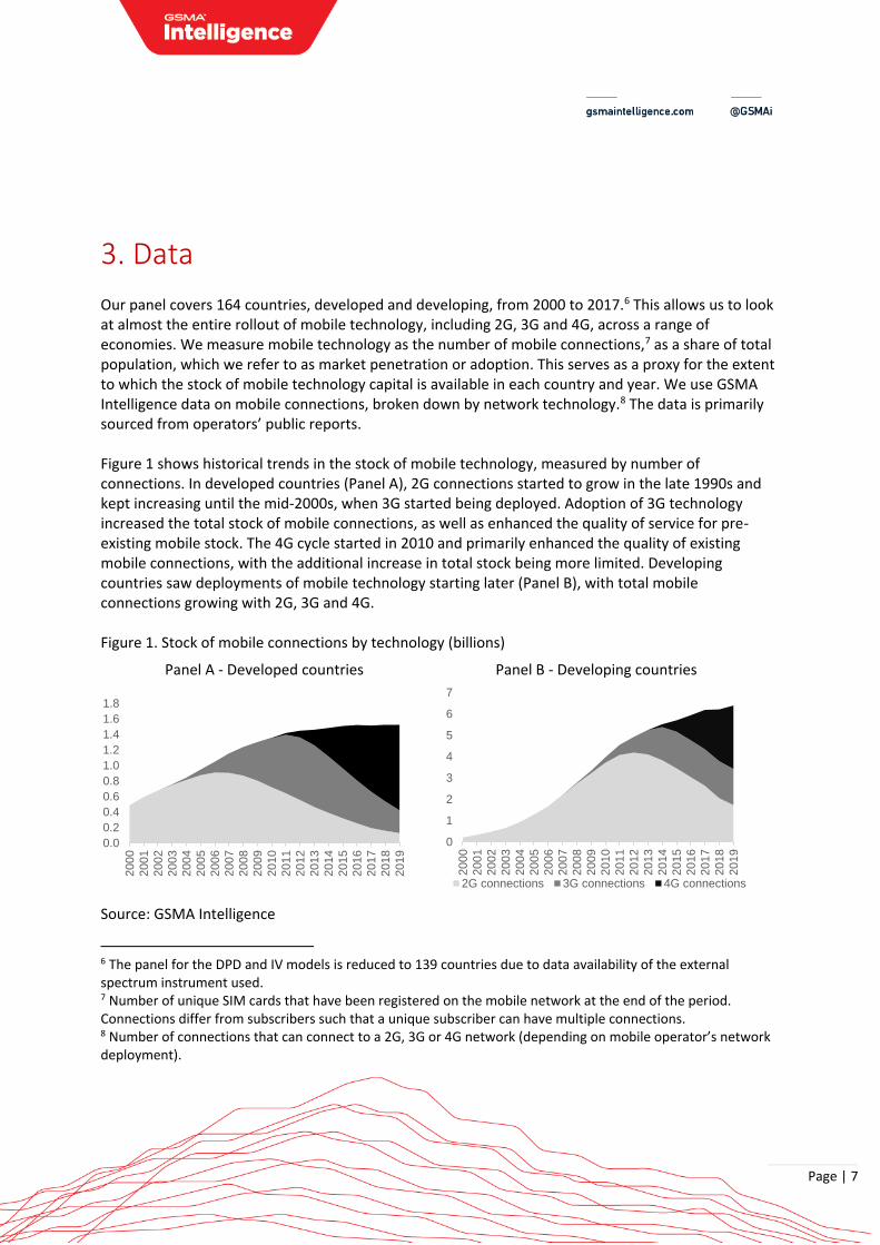
3. Data Our panel covers 164 countries, developed and developing, from 2000 to 2017.6 This allows us to look at almost the entire rollout of mobile technology, including 2G, 3G and 4G, across a range of economies. We measure mobile technology as the number of mobile connections,7 as a share of total population, which we refer to as market penetration or adoption. This serves as a proxy for the extent to which the stock of mobile technology capital is available in each country and year. We use GSMA Intelligence data on mobile connections, broken down by network technology.8 The data is primarily sourced from operators’ public reports. Figure 1 shows historical trends in the stock of mobile technology, measured by number of connections. In developed countries (Panel A), 2G connections started to grow in the late 1990s and kept increasing until the mid-2000s, when 3G started being deployed. Adoption of 3G technology increased the total stock of mobile connections, as well as enhanced the quality of service for pre-existing mobile stock. The 4G cycle started in 2010 and primarily enhanced the quality of existing mobile connections, with the additional increase in total stock being more limited. Developing countries saw deployments of mobile technology starting later (Panel B), with total mobile connections growing with 2G, 3G and 4G. Figure 1. Stock of mobile connections by technology (billions)

Panel A - Developed countries Panel B - Developing countries

Source: GSMA Intelligence

6 The panel for the DPD and IV models is reduced to 139 countries due to data availability of the external spectrum instrument used. 7 Number of unique SIM cards that have been registered on the mobile network at the end of the period. Connections differ from subscribers such that a unique subscriber can have multiple connections. 8 Number of connections that can connect to a 2G, 3G or 4G network (depending on mobile operator’s network deployment).

0.0

0.2

0.4

0.6

0.8

1.0

1.2

1.4

1.6

1.8

200

0

200

1

200

2

200

3

200

4

200

5

200

6

200

7

200

8

200

9

201

0

201

1

201

2

201

3

201

4

201

5

201

6

201

7

201

8

201

9

0

1

2

3

4

5

6

7

200

0

200

1

200

2

200

3

200

4

200

5

200

6

200

7

200

8

200

9

201

0

201

1

201

2

201

3

201

4

20

15

201

6

201

7

201

8

201

9

2G connections 3G connections 4G connections

Page | 8

4. Empirical strategy

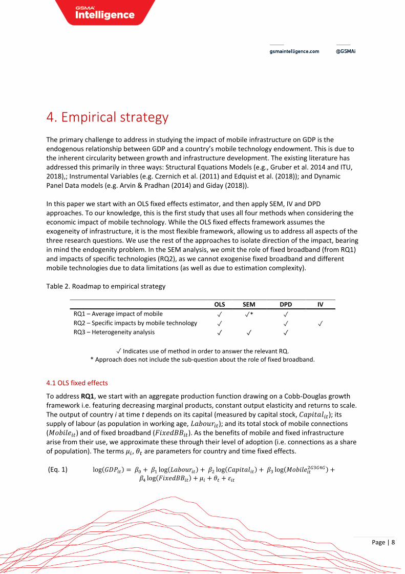
The primary challenge to address in studying the impact of mobile infrastructure on GDP is the endogenous relationship between GDP and a country’s mobile technology endowment. This is due to the inherent circularity between growth and infrastructure development. The existing literature has addressed this primarily in three ways: Structural Equations Models (e.g., Gruber et al. 2014 and ITU, 2018),; Instrumental Variables (e.g. Czernich et al. (2011) and Edquist et al. (2018)); and Dynamic Panel Data models (e.g. Arvin & Pradhan (2014) and Giday (2018)). In this paper we start with an OLS fixed effects estimator, and then apply SEM, IV and DPD approaches. To our knowledge, this is the first study that uses all four methods when considering the economic impact of mobile technology. While the OLS fixed effects framework assumes the exogeneity of infrastructure, it is the most flexible framework, allowing us to address all aspects of the three research questions. We use the rest of the approaches to isolate direction of the impact, bearing in mind the endogenity problem. In the SEM analysis, we omit the role of fixed broadband (from RQ1) and impacts of specific technologies (RQ2), as we cannot exogenise fixed broadband and different mobile technologies due to data limitations (as well as due to estimation complexity). Table 2. Roadmap to empirical strategy

OLS SEM DPD IV

RQ1 – Average impact of mobile ✓ ✓* ✓

RQ2 – Specific impacts by mobile technology ✓ ✓ ✓ RQ3 – Heterogeneity analysis ✓ ✓ ✓

✓ Indicates use of method in order to answer the relevant RQ. * Approach does not include the sub-question about the role of fixed broadband.

4.1 OLS fixed effects

To address RQ1, we start with an aggregate production function drawing on a Cobb-Douglas growth framework i.e. featuring decreasing marginal products, constant output elasticity and returns to scale. The output of country i at time t depends on its capital (measured by capital stock, 𝐶𝑎𝑝𝑖𝑡𝑎𝑙𝑖𝑡); its supply of labour (as population in working age, 𝐿𝑎𝑏𝑜𝑢𝑟𝑖𝑡); and its total stock of mobile connections (𝑀𝑜𝑏𝑖𝑙𝑒𝑖𝑡) and of fixed broadband (𝐹𝑖𝑥𝑒𝑑𝐵𝐵𝑖𝑡). As the benefits of mobile and fixed infrastructure arise from their use, we approximate these through their level of adoption (i.e. connections as a share of population). The terms 𝜇𝑖, 𝜃𝑡 are parameters for country and time fixed effects. (Eq. 1) log(𝐺𝐷𝑃𝑖𝑡) = 𝛽0 + 𝛽1 log(𝐿𝑎𝑏𝑜𝑢𝑟𝑖𝑡) + 𝛽2 log(𝐶𝑎𝑝𝑖𝑡𝑎𝑙𝑖𝑡) + 𝛽3 log(𝑀𝑜𝑏𝑖𝑙𝑒𝑖𝑡

2𝐺3𝐺4𝐺) + 𝛽4 log(𝐹𝑖𝑥𝑒𝑑𝐵𝐵𝑖𝑡) + 𝜇𝑖 + 𝜃𝑡 + 휀𝑖𝑡

Page | 9

To test how the results varied over time, we break down the average impact of mobile by its effects in three periods of infrastructure development: (i) early deployments; (ii) early mobile internet; and (iii)

fast networks. We operationalise this by interacting 𝑀𝑜𝑏𝑖𝑙𝑒𝑖𝑡2𝐺3𝐺4𝐺 with three country-specific,

mutually exclusive dummies in the aggregate production function (Equation 2). 𝐸𝑎𝑟𝑙𝑦𝐷𝑒𝑝𝑙𝑜𝑦𝑚𝑒𝑛𝑡𝑠𝑖𝑡 is a dummy taking value 1 from the time when 2G started being adopted until the time 3G first became available, or 0 otherwise. The 𝐸𝑎𝑟𝑙𝑦𝑀𝑜𝑏𝑖𝑙𝑒𝐼𝑛𝑡𝑒𝑟𝑛𝑒𝑡𝑖𝑡 dummy covers from the start of the 3G cycle to the start of 4G being rolled out, and the 𝐹𝑎𝑠𝑡𝑁𝑒𝑡𝑤𝑜𝑟𝑘𝑠𝑖𝑡 variable covers the time thereafter.9 The coefficients will therefore recover the impact of increasing the total stock of mobile connections in different periods of mobile innovation. (Eq. 2) 𝑙𝑜𝑔(𝐺𝐷𝑃𝑖𝑡) = 𝛽0 + 𝛽1 log(𝐶𝑎𝑝𝑖𝑡𝑎𝑙𝑖𝑡) + 𝛽2 log(𝐿𝑎𝑏𝑜𝑢𝑟𝑖𝑡) + 𝛽3 log(𝑀𝑜𝑏𝑖𝑙𝑒𝑖𝑡

2𝐺3𝐺4𝐺) ∗ (𝐸𝑎𝑟𝑙𝑦𝐷𝑒𝑝𝑙𝑜𝑦𝑚𝑒𝑛𝑡𝑠𝑖𝑡 + 𝐸𝑎𝑟𝑙𝑦𝑀𝑜𝑏𝑖𝑙𝑒𝐼𝑛𝑡𝑒𝑟𝑛𝑒𝑡𝑖𝑡 + 𝐹𝑎𝑠𝑡𝑁𝑒𝑡𝑤𝑜𝑟𝑘𝑠𝑖𝑡) + + 𝛽4 log(𝐹𝑖𝑥𝑒𝑑𝑏𝑏𝑖𝑡) 𝜇𝑖 + 𝜃𝑡 + 휀𝑖𝑡

Regarding RQ2, disentangling the impact of different technology generations is a challenging task because the change on the type of mobile services is not linear between mobile technology generations.10 In this paper, we propose using three cumulative building blocks. Equation 3 includes

the total stock of mobile connections (𝑀𝑜𝑏𝑖𝑙𝑒𝑖𝑡2𝐺3𝐺4𝐺); that of 3G and 4G networks (𝑀𝑜𝑏𝑖𝑙𝑒𝑖𝑡

3𝐺4𝐺); and

that of 4G connections (𝑀𝑜𝑏𝑖𝑙𝑒𝑖𝑡4𝐺). Estimating these three variables in the same equation means that

𝛾3, 𝛾4 and 𝛾5 will allow us to capture technology impacts, as explained below. (Eq. 3) log(𝐺𝐷𝑃𝑖𝑡) = 𝛾0 + 𝛾1 log(𝐿𝑎𝑏𝑜𝑢𝑟𝑖𝑡) + 𝛾2 log(𝐶𝑎𝑝𝑖𝑡𝑎𝑙𝑖𝑡)

+ 𝛾3 log(𝑀𝑜𝑏𝑖𝑙𝑒𝑖𝑡2𝐺3𝐺4𝐺) + 𝛾4 log(𝑀𝑜𝑏𝑖𝑙𝑒𝑖𝑡

3𝐺4𝐺) + 𝛾5 log(𝑀𝑜𝑏𝑖𝑙𝑒𝑖𝑡4𝐺)

+ 𝛾6 log(𝐹𝑖𝑥𝑒𝑑𝑏𝑏𝑖𝑡) + 𝜇𝑖 + 𝜃𝑡 + 휀𝑖𝑡 Firstly, 𝛾3 will recover the impact of increasing the total stock of mobile connections, holding constant the increases in 3G and 4G. This therefore represents the impact of gaining 2G, or basic mobile connectivity – we refer to this as the connectivity effect.

9 We define these dummies using mobile penetration variables, so that 𝐸𝑎𝑟𝑙𝑦𝐷𝑒𝑝𝑙𝑜𝑦𝑚𝑒𝑛𝑡𝑠𝑖𝑡 covers the period until 3G mobile penetration is positive; 𝐸𝑎𝑟𝑙𝑦𝑀𝑜𝑏𝑖𝑙𝑒𝐼𝑛𝑡𝑒𝑟𝑛𝑒𝑡𝑖𝑡 spans from the latter until 4G penetration is positive; and 𝐹𝑎𝑠𝑡𝑁𝑒𝑡𝑤𝑜𝑟𝑘𝑠𝑖𝑡, the rest. We have done sensitivities where these dummies take value 1 where mobile connections penetration surpass 1% and 5% thresholds, with results being broadly consistent. This approach is based on Koutroumpis (2016). 10 After a given technology has been rolled out, the start of the deployment of a new technology means that the former will be partly replaced i.e. connections on the former infrastructure tend to decrease. In particular, the 2G and 3G variables’ impact would be estimated in the parts of the panel where their penetration decreases, as they are substituted by subsequent generations. At the same time, the timeline of rollout of these technologies partly overlaps (particularly for 2G and 3G), meaning they are collinear to some extent. Ultimately, in Equation 1,

this means we cannot simply replace 𝑀𝑜𝑏𝑖𝑙𝑒𝑖𝑡2𝐺3𝐺4𝐺 by three variables individually capturing 2G, 3G and 4G, as

their impacts would be confounded.

Page | 10

Secondly, holding the total stock of mobile connections constant, 𝛾4 and 𝛾5 will retrieve upgrade effects arising from existing connections transiting to 3G and 4G. In particular, the term 𝛾4 measures

the impact of increasing 𝑀𝑜𝑏𝑖𝑙𝑒𝑖𝑡3𝐺4𝐺 ceteris paribus (including total stock of connections as well as

𝑀𝑜𝑏𝑖𝑙𝑒𝑖𝑡4𝐺), so will necessarily capture additional benefits brought by existing 2G connections

upgrading to 3G services. Meanwhile, 𝛾5 will capture benefits of increasing 𝑀𝑜𝑏𝑖𝑙𝑒𝑖𝑡4𝐺 keeping the rest

constant, or the impact of existing 3G connections upgrading to 4G. Regarding the heterogeneity analysis (RQ3), to assess the role of take-up we modify the basic aggregate production function (Equation 1) adding interactions of mobile with adoption level dummies for low, medium and high take-up (as per the 33th and 66th percentiles of the distribution of the data, corresponding to 43% and 97%, respectively).11 To evaluate differences created by skills, economic structure and income, we follow two approaches. First, we run regressions on sample splits. These divide the panel in countries above and below median values of years of schooling (9 years), to assess the role of skills; share of services and manufacturing sectors in employment (75%), to assess the role of economic structure; and developed and developing countries12, to analyse the role of income. Second, to provide reassurance of statistical significance of the differences between samples, 13 we also estimate models interacting mobile adoption with a dummy taking value 1 when years of schooling are above the median, for the analysis on impact of skills; and with a dummy taking value 1 when share of services and manufacturing sectors in employment is above the median, for the analysis of the effect of economic structure.

4.2 Structural Equations Model

To isolate the causal impact of mobile infrastructure on GDP, we use a Structural Equations Model.14 This specifies a micro-model for the mobile sector in each country, consisting of equations for the demand and supply of mobile infrastructure, as well as an infrastructure function. This framework allows us to endogenise mobile technology because it incorporates the structural, fundamental drivers of the mobile infrastructure market (including GDP).

11 This approach is consistent with related wider research on telecommunications infrastructure that has also looked at the role of take-up (for example, see Koutroumpis 2009). 12 We regard as developed countries those categorised as high-income countries as per the World Bank groupings – developing otherwise. <https://datahelpdesk.worldbank.org/knowledgebase/articles/906519-world-bank-country-and-lending-groups>. 13 While sample splits provide a flexible framework allowing for sample-specific estimates for independent variables, we note this comes at the expense of making the assessment of statistical significance of differences in coefficients (from separate regressions) challenging. The latter is addressed through the interaction approach. 14 We implement this with Stata’s gmm command, which allows for robust standard errors clusters by country.

https://datahelpdesk.worldbank.org/knowledgebase/articles/906519-world-bank-country-and-lending-groups

https://datahelpdesk.worldbank.org/knowledgebase/articles/906519-world-bank-country-and-lending-groups

Page | 11

We omit unpicking the specific role of each mobile technology generation (RQ2) and the role of fixed broadband (part of RQ1), as this would require embedding additional SEMs – something we could not do due to data limitations to estimate demand, supply and infrastructure equations and due to estimation complexity.15 We apply a SEM model including country and time fixed effects on all equations. This broadly follows the approach extensively used in the literature – see Roller and Waverman (2001), Gruber and Koutroumpis (2011), Gruber et al. (2014), Koutroumpis (2009, 2016 and 2018) and ITU (2018). It features an aggregate production function similar to that of Equation 1, providing the baseline average impact of mobile infrastructure (RQ1). Note we also adjust this equation inserting the three country-specific, mutually exclusive dummies, to assess how this effect varies over time (as in Equation 2). (Eq. 4) Aggregate production log (𝐺𝐷𝑃𝑖𝑡) = 𝛽0 + 𝛽1log(𝐶𝑎𝑝𝑖𝑡𝑎𝑙𝑖𝑡) + 𝛽2log(𝐿𝑎𝑏𝑜𝑢𝑟𝑖𝑡) +

𝛽3log (𝑀𝑜𝑏𝑖𝑙𝑒𝑖𝑡2𝐺3𝐺4𝐺) + 𝜇𝑖 + 𝜃𝑡 + 휀𝑖𝑡

(Eq. 5) Demand function log (𝑀𝑜𝑏𝑖𝑙𝑒𝑖𝑡2𝐺3𝐺4𝐺) = 𝜃0 + 𝜃1log (𝐺𝐷𝑃𝑐𝑎𝑝𝑖𝑡𝑎𝑖𝑡) + 𝜃2log(𝐴𝑅𝑃𝑈𝑖𝑡) +

𝜃3log(𝑈𝑟𝑏𝑎𝑛𝑖𝑧𝑎𝑡𝑖𝑜𝑛𝑖𝑡) + 𝜇𝑖 + 𝜃𝑡 + 휀𝑖𝑡 (Eq. 6) Supply function log(𝐶𝑎𝑝𝑒𝑥𝑖𝑡) = 𝜌0 + 𝜌1log(𝐺𝐷𝑃𝑐𝑎𝑝𝑖𝑡𝑎𝑖𝑡) + 𝜃2log(𝑈𝑟𝑏𝑎𝑛𝑖𝑧𝑎𝑡𝑖𝑜𝑛𝑖𝑡) + 𝜃3log(𝐻𝐻𝐼𝑖𝑡) + 𝜇𝑖 + 𝜃𝑡 + 휀𝑖𝑡

(Eq. 7) Mobile infrastructure log(∆𝑀𝑜𝑏𝑖𝑙𝑒𝑖𝑡2𝐺3𝐺4𝐺) = 𝛿0 + 𝛿1log(𝐶𝑎𝑝𝑒𝑥𝑖𝑡) + 𝜇𝑖 + 𝜃𝑡 + 휀𝑖𝑡

The demand equation (Equation 5) captures changes in mobile penetration that are driven by income (as per GDP per capita, 𝐿𝑜𝑔𝐺𝐷𝑃𝑐𝑎𝑝𝑖𝑡𝑎𝑖𝑡); the prices of mobile services (proxied by average revenue per user, 𝐿𝑜𝑔𝐴𝑅𝑃𝑈𝑖𝑡); and the propensity to adopt mobile technology as per urbanisation levels (share of urban population, 𝐿𝑜𝑔𝑈𝑟𝑏𝑎𝑛𝑖𝑧𝑎𝑡𝑖𝑜𝑛𝑖𝑡). The supply model (Equation 6) implies that investment in mobile infrastructure (capital expenditures, 𝐿𝑜𝑔𝐶𝑎𝑝𝑒𝑥𝑖𝑡) depends on income per capita, as a measure of willingness to pay; the costs for rolling out, which are typically shifted by the population distribution, and we approximate through urbanisation levels; as well as the degree of market concentration (𝐿𝑜𝑔𝐻𝐻𝐼𝑖𝑡), as a measure of the intensity of competition among firms.

15 Accounting for 2G-, 3G- and 4G-specific effects would require technology-specific data for the demand, supply and infrastructure equations, something that is not available to us. For fixed broadband, although there is pricing and investment data from different sources, this only covers part of our panel. Moreover, inserting three built-in equations for each mobile technology generation or for fixed broadband would mean estimating many more equations – which would increase the complexity of the estimation and be very demanding for the variation of the data.

Page | 12

Finally, the infrastructure equation (Equation 7) states that the change in mobile penetration depends on investment in mobile infrastructure, as measured by capital expenditures, as this is typically the main source for funding infrastructure growth for mobile operators. Note Equations 3–6 also allow for country and time fixed effects 𝜇𝑖 and 𝜃𝑡, as in the OLS framework.

4.3 Instrumental Variable

We evaluate the robustness of findings using instrumental variables, which also exogenises the stock of mobile connections. As an external instrument, we use the spectrum assigned to mobile operators by governments. This is because, in order to launch mobile networks, operators need to be able to use radio frequencies over the airwaves, or spectrum. The amount of spectrum holdings drives not only the availability of mobile services but also the quality of these, while it should be exogenous relative to GDP (particularly across countries of similar development levels).16 However, due to the availability of data, we can only capture spectrum assigned to 3G and 4G technology. We run a 2SLS regression with country and time fixed effects, evaluating the impact of the

𝑀𝑜𝑏𝑖𝑙𝑒𝑖𝑡3𝐺4𝐺 variable on 𝐺𝐷𝑃𝑖𝑡, with the first stage defining 𝑀𝑜𝑏𝑖𝑙𝑒𝑖𝑡

3𝐺4𝐺 as a function of the amount of spectrum available for 3G and 4G mobile services in each country and year. As we do not control for

the total stock of mobile connections in this framework, the parameter for 𝑀𝑜𝑏𝑖𝑙𝑒𝑖𝑡3𝐺4𝐺 can be

interpreted as partly aggregating both connectivity and upgrade effects – as growth in 3G and 4G connections has not only upgraded 2G connections but also increased the total stock of connections in parts of our panel. This IV 2SLS strategy allows us to check the robustness of our results for technology-specific impacts (RQ2), which we are unable to do in the SEM framework.

4.4 Dynamic Panel Data

As a final robustness check on the results for each research question, we apply a Dynamic Panel Data model with Arellano Bond estimators. As done in the related literature using DPD models, we add a partial adjustment mechanism (specifically, the first lag of GDP), common in growth models to better account for macroeconomic time series.17 Adding this term effectively means that impact estimates will be read as the elasticity of the GDP growth rate with respect to mobile, rather than the elasticity of the GDP level relative to mobile (as in OLS and SEM results). Regarding instruments, we implement the third lag of internal instruments, as well as the external, exogenous spectrum variable discussed in Section 4.3.

16 Countries have assigned mobile spectrum for different mobile technologies at different points in time, giving substantial variation in the instrument. 17 We apply a difference GMM estimator, using Stata’s command xtabond2.

Page | 13

5. Results 5.1 Average impact of mobile (RQ1)

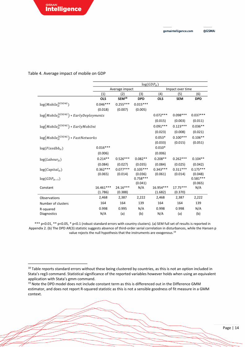
Our OLS and SEM analysis for the average impact of mobile (columns 1–3 in Table 4) suggests that a 10% increase in the adoption of mobile technology drives an increase in GDP from 0.46% to 2.55%. While this is a wide range, we note it is broadly consistent with the existing literature. Having said that, we treat the upper bound of the SEM result with some caution, as the effect may be confounded by the capital variable, which has a small impact compared to the results in this set of outputs (and elsewhere in this paper). Our DPD setting confirms the direction of this effect, relative to the GDP growth rate. Columns 4–6 test whether this average impact has significantly varied over time. Taking into account standard errors, with a 95% confidence interval we note that OLS, SEM and DPD results are overlapping over the three time periods. This suggests that impacts have likely been fairly stable over the three periods evaluated. In particular, OLS and SEM point to a 10% in mobile generating returns to GDP from 0.5% to 1.2% – with results of both approaches here pointing to a narrower range of impacts. Overall, we can conclude that benefits brought by mobile technology have remained stable at this range of 0.5% to 1.2% (RQ1).

Page | 14

Table 4. Average impact of mobile on GDP

log(𝐺𝐷𝑃𝑖𝑡)

Average impact Impact over time

(1) (2) (3) (4) (5) (6)

OLS SEM18 DPD OLS SEM DPD

log(𝑀𝑜𝑏𝑖𝑙𝑒𝑖𝑡2𝐺3𝐺4𝐺) 0.046*** 0.255*** 0.015***

(0.018) (0.007) (0.005)

log(𝑀𝑜𝑏𝑖𝑙𝑒𝑖𝑡2𝐺3𝐺4𝐺) ∗ 𝐸𝑎𝑟𝑙𝑦𝐷𝑒𝑝𝑙𝑜𝑦𝑚𝑒𝑛𝑡𝑠 0.072*** 0.098*** 0.037***

(0.015) (0.003) (0.011)

log(𝑀𝑜𝑏𝑖𝑙𝑒𝑖𝑡2𝐺3𝐺4𝐺) ∗ 𝐸𝑎𝑟𝑙𝑦𝑀𝑜𝑏𝑖𝐼𝑛𝑡 0.091*** 0.123*** 0.036**

(0.023) (0.008) (0.021)

log(𝑀𝑜𝑏𝑖𝑙𝑒𝑖𝑡2𝐺3𝐺4𝐺) ∗ 𝐹𝑎𝑠𝑡𝑁𝑒𝑡𝑤𝑜𝑟𝑘𝑠 0.053* 0.100*** 0.106**

(0.033) (0.015) (0.051)

log(𝐹𝑖𝑥𝑒𝑑𝑏𝑏𝑖𝑡) 0.016*** 0.010*

(0.006) (0.006)

log(𝐿𝑎𝑏𝑜𝑢𝑟𝑖𝑡) 0.214** 0.526*** 0.082** 0.208** 0.262*** 0.104**

(0.084) (0.027) (0.035) (0.084) (0.025) (0.042)

log(𝐶𝑎𝑝𝑖𝑡𝑎𝑙𝑖𝑡) 0.362*** 0.077*** 0.105*** 0.343*** 0.311*** 0.175***

(0.065) (0.014) (0.036) (0.061) (0.014) (0.048)

log(𝐺𝐷𝑃𝑖𝑡−1) 0.758*** 0.581*** (0.041) (0.065) Constant 16.461*** 24.16*** N/A 16.954*** 17.75*** N/A (1.786) (0.388) (1.682) (0.370)

Observations 2,468 2,387 2,222 2,468 2,387 2,222

Number of clusters 164 164 139 164 164 139

R-squared 0.998 0.995 N/A 0.998 0.998 N/A

Diagnostics N/A (a) (b) N/A (a) (b)

*** p<0.01, ** p<0.05, * p<0.1 (robust standard errors with country clusters). (a) SEM full set of results is reported in

Appendix 2. (b) The DPD AR(3) statistic suggests absence of third-order serial correlation in disturbances, while the Hansen p value rejects the null hypothesis that the instruments are exogenous.19

18 Table reports standard errors without these being clustered by countries, as this is not an option included in Stata’s reg3 command. Statistical significance of the reported variables however holds when using an equivalent application with Stata’s gmm command. 19 Note the DPD model does not include constant term as this is differenced out in the Difference GMM estimator, and does not report R-squared statistic as this is not a sensible goodness of fit measure in a GMM context.

Page | 15

We note our OLS FE estimates for mobile variables remain significant after accounting for fixed broadband, so we can conclude that impacts of mobile technology materialise above effects driven by fixed infrastructure. We have run additional analyses using the internal instruments provided by the DPD framework (allowing us to instrument both mobile and fixed broadband), with results being in the same direction.20 Regarding diagnostics, labour and capital have the expected significant effects.21 For the rest, in the SEM, the drivers of demand, supply and mobile infrastructure functions are all significant and in the expected directions (see Appendix 2)22; and the DPD test for autocorrelation suggests errors are not autocorrelated (however, we note a low value of the Hansen p value, suggesting that the instruments may not be exogenous).

5.2 Specific impacts by technologies (RQ2)

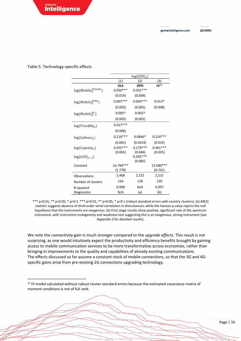
The analysis of impacts by technologies is reported in columns 1–3 in Table 5. Increasing the total stock of mobile connections by 10% drives an increase in GDP of 0.50% in our OLS setting, with the DPD framework also confirming a significant impact. As this coefficient measures the impact of the

total stock of connections ceteris paribus (including keeping 𝑀𝑜𝑏𝑖𝑙𝑒𝑖𝑡3𝐺4𝐺 and 𝑀𝑜𝑏𝑖𝑙𝑒𝑖𝑡

4𝐺 constant), we interpret this as the impact of basic 2G connectivity, or a baseline connectivity effect.

Importantly, we also find statistical significance in 𝑀𝑜𝑏𝑖𝑙𝑒𝑖𝑡3𝐺4𝐺 and 𝑀𝑜𝑏𝑖𝑙𝑒𝑖𝑡

4𝐺 , suggesting growth in 3G and 4G connections generates additional impacts on top of the baseline connectivity effect. Note these effects are found while keeping the stock of connections constant, meaning these benefits arise from existing connections being transitioned from 2G to 3G, and from 3G to 4G i.e. upgrade effects.

Firstly, for 3G, the OLS framework finds that increasing 𝑀𝑜𝑏𝑖𝑙𝑒𝑖𝑡3𝐺4𝐺 by 10% (holding 𝑀𝑜𝑏𝑖𝑙𝑒𝑖𝑡

4𝐺 fixed), raises mobile’s impact on GDP by 0.07 percentage points – with the DPD result also being consistent.

Secondly, ceteris paribus, raising 𝑀𝑜𝑏𝑖𝑙𝑒𝑖𝑡4𝐺 by 10% percent further raises mobile’s GDP impact 0.05

percentage points in the OLS model, with a finding in similar direction in the dynamic model. Overall, the above means that mobile’s baseline impact coefficient of 0.05 increases by about 15% when connections are upgraded to 3G. For connections upgrading from 2G to 4G, the impact increases by approximately 25%.

20 Results available in Appendix 4. 21 Apart from the already discussed magnitude capital in the SEM model in column 2, we also note that the DPD labour and capital coefficient magnitudes tend to be distinct (in these results and elsewhere in the paper), simply due to these effects being partly picked up by the GDP lag. 22 The demand equation shows expected, significant drivers: a negative role for ARPU (with a PED in the inelastic range of 0 to 1, as one expects with necessity goods); positive income elasticity; and a positive effect of urbanisation. The supply results show a positive role for income and for urbanisation, with HHI being a negative significant driver. The mobile infrastructure function, as expected, is positively affected by investment.

Page | 16

Table 5. Technology-specific effects


(1) (2) (3)

OLS DPD IV23

log(𝑀𝑜𝑏𝑖𝑙𝑒𝑖𝑡2𝐺3𝐺4𝐺) 0.050*** 0.031***

(0.019) (0.009)

log(𝑀𝑜𝑏𝑖𝑙𝑒𝑖𝑡3𝐺4𝐺) 0.007*** 0.004*** 0.013*

(0.002) (0.001) (0.008)

log(𝑀𝑜𝑏𝑖𝑙𝑒𝑖𝑡4𝐺) 0.005* 0.002*

(0.003) (0.001)

log(𝐹𝑖𝑥𝑒𝑑𝑏𝑏𝑖𝑡) 0.017***

(0.006)

log(𝐿𝑎𝑏𝑜𝑢𝑟𝑖𝑡) 0.216*** 0.0846* 0.214***

(0.081) (0.0433) (0.033)

log(𝐶𝑎𝑝𝑖𝑡𝑎𝑙𝑖𝑡) 0.355*** 0.179*** 0.461***

(0.065) (0.046) (0.025)

log(𝐺𝐷𝑃𝑖𝑡−1) 0.505*** (0.085) Constant 16.794*** 13.580*** (1.778) (0.701)

Observations 2,468 2,222 2,222

Number of clusters 164 139 139

R-squared 0.998 N/A 0.997

Diagnostics N/A (a) (b)

*** p<0.01, ** p<0.05, * p<0.1. *** p<0.01, ** p<0.05, * p<0.1 (robust standard errors with country clusters). (a) AR(3)

statistic suggests absence of third-order serial correlation in disturbances, while the Hansen p value rejects the null hypothesis that the instruments are exogenous. (b) First stage results show positive, significant role of the spectrum instrument, with instrument endogeneity and weakness test suggesting this is an exogenous, strong instrument (see

Appendix 3 for detailed results).

We note the connectivity gain is much stronger compared to the upgrade effects. This result is not surprising, as one would intuitively expect the productivity and efficiency benefits brought by gaining access to mobile communication services to be more transformative across economies, rather than bringing in improvements to the quality and capabilities of already existing communications. The effects discussed so far assume a constant stock of mobile connections, so that the 3G and 4G-specific gains arise from pre-existing 2G connections upgrading technology.

23 IV model calculated without robust cluster standard errors because the estimated covariance matrix of moment conditions is not of full rank.

Page | 17

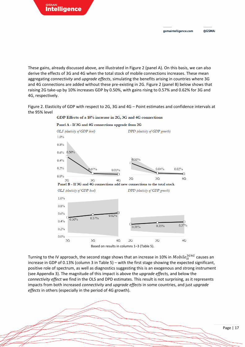
These gains, already discussed above, are illustrated in Figure 2 (panel A). On this basis, we can also derive the effects of 3G and 4G when the total stock of mobile connections increases. These mean aggregating connectivity and upgrade effects, simulating the benefits arising in countries where 3G and 4G connections are added without these pre-existing in 2G. Figure 2 (panel B) below shows that raising 2G take-up by 10% increases GDP by 0.50%, with gains rising to 0.57% and 0.62% for 3G and 4G, respectively. Figure 2. Elasticity of GDP with respect to 2G, 3G and 4G – Point estimates and confidence intervals at the 95% level

Based on results in columns 1–3 (Table 5).

Turning to the IV approach, the second stage shows that an increase in 10% in 𝑀𝑜𝑏𝑖𝑙𝑒𝑖𝑡3𝐺4𝐺 causes an

increase in GDP of 0.13% (column 3 in Table 5) – with the first stage showing the expected significant, positive role of spectrum, as well as diagnostics suggesting this is an exogenous and strong instrument (see Appendix 3). The magnitude of this impact is above the upgrade effects, and below the connectivity effect we find in the OLS and DPD estimates. This result is not surprising, as it represents impacts from both increased connectivity and upgrade effects in some countries, and just upgrade effects in others (especially in the period of 4G growth).

Page | 18

Overall, we can therefore conclude that the rollout of subsequent mobile network generations increases the economic impact of mobile on GDP (RQ2). The significant upgrade effects of 3G and 4G especially point to the role of improvements in mobile data service quality in increasing mobile’s impact on GDP (especially improvements in upload, download speeds and latency). Regarding the specific impacts found, if we take confidence intervals into account, these are broadly consistent with the impact found for the average impact of mobile (RQ1).

5.3 Heterogeneity analysis (RQ3)

The role of network effects

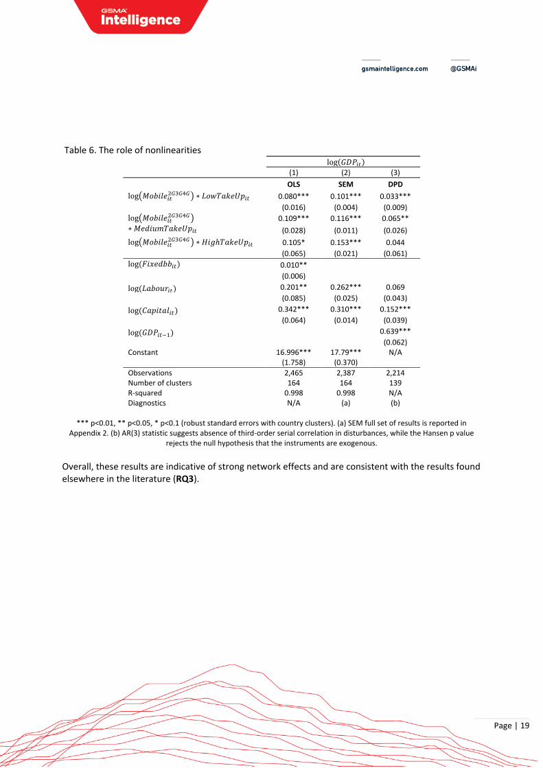
With positive network externalities, returns to mobile networks should increase the more users adopt mobile services. This phenomenon has been reported in related literature. For example, Roller and Waverman (2001) found that fixed wireline impacts are only significant with penetration rates above 40%, while broadband adoption has been found to have lower thresholds, from 10% to 30% (Czernich et al. (2009), Gruber et al. (2014), Koutroumpis (2009)). Gruber & Koutroumpis (2011) found increases in impacts of mobile when this surpasses 30–40% of adoption. Our results confirm the existence of nonlinearities, with mobile impacts increasing with the adoption level dummies for low, medium and high take-up. OLS and SEM analysis suggest increasing impacts once mobile population penetration surpasses the 43% and 97% thresholds, which correspond to the medium and high take-up levels (columns 1–2 in Table 6), while DPD results point to nonlinearities being significant only at low to middle levels of mobile adoption (column 3). In particular, looking at GDP level impacts (OLS and SEM): for low levels of take-up, a 10% increase in mobile adoption drives an increase of GDP of 0.80–1.01%; for medium take-up, impacts increase to 1.09–1.16%; and reach 1.05-1.53% at high levels of adoption.

Page | 19

Table 6. The role of nonlinearities log(𝐺𝐷𝑃𝑖𝑡)

(1) (2) (3)

OLS SEM DPD

log(𝑀𝑜𝑏𝑖𝑙𝑒𝑖𝑡2𝐺3𝐺4𝐺) ∗ 𝐿𝑜𝑤𝑇𝑎𝑘𝑒𝑈𝑝𝑖𝑡 0.080*** 0.101*** 0.033***

(0.016) (0.004) (0.009)

log(𝑀𝑜𝑏𝑖𝑙𝑒𝑖𝑡2𝐺3𝐺4𝐺)

∗ 𝑀𝑒𝑑𝑖𝑢𝑚𝑇𝑎𝑘𝑒𝑈𝑝𝑖𝑡 0.109*** 0.116*** 0.065**

(0.028) (0.011) (0.026)

log(𝑀𝑜𝑏𝑖𝑙𝑒𝑖𝑡2𝐺3𝐺4𝐺) ∗ 𝐻𝑖𝑔ℎ𝑇𝑎𝑘𝑒𝑈𝑝𝑖𝑡 0.105* 0.153*** 0.044

(0.065) (0.021) (0.061)

log(𝐹𝑖𝑥𝑒𝑑𝑏𝑏𝑖𝑡) 0.010**

(0.006)

log(𝐿𝑎𝑏𝑜𝑢𝑟𝑖𝑡) 0.201** 0.262*** 0.069

(0.085) (0.025) (0.043)

log(𝐶𝑎𝑝𝑖𝑡𝑎𝑙𝑖𝑡) 0.342*** 0.310*** 0.152***

(0.064) (0.014) (0.039)

log(𝐺𝐷𝑃𝑖𝑡−1) 0.639***

(0.062) Constant 16.996*** 17.79*** N/A

(1.758) (0.370)

Observations 2,465 2,387 2,214 Number of clusters 164 164 139 R-squared 0.998 0.998 N/A Diagnostics N/A (a) (b)


Appendix 2. (b) AR(3) statistic suggests absence of third-order serial correlation in disturbances, while the Hansen p value rejects the null hypothesis that the instruments are exogenous.

Overall, these results are indicative of strong network effects and are consistent with the results found elsewhere in the literature (RQ3).

Page | 20

The role of skills

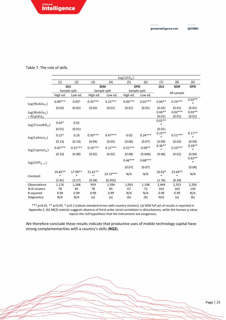
Countries with skilled labour tend to enjoy greater impacts from ICT, as this allows them to better absorb telecoms capital. For example, pre-existing human capital increases the impact of broadband on firm creation and wage growth24; and regions that have thicker labour markets for complementary services also experience stronger benefits out of broadband (Forman et al. (2012)). This question has been less addressed with respect to mobile technology specifically, though some studies have indicated this is likely the case.25 To explore whether mobile technologies have complementarities with human capital, Table 7 shows regressions for the “High education” and “Low education” subsamples, based on the median of 9 years of average schooling (columns 1–6 in Table 7). This analysis unambiguously points to significantly greater impacts in countries with higher education levels on average. Specifically, the magnitude of our point estimates for high education countries are 1.6 to 3 times those that we see in the sample for low education countries, depending on the approach – suggesting substantial differences. The interaction approach – where we interact mobile with a dummy taking value 1 when a country has more years of schooling than the median (𝐻𝑖𝑔ℎ𝐸𝑑𝑖𝑡) – provides similar insights in all OLS, SEM and DPD frameworks (columns 7–9), with the dummy variable being significant.

24 See McCoy et al. (2017); Forman et al. (2012); Atasoy (2013); Mack and Faggian (2013). 25 For example, Giday (2018) found low impacts of mobile internet in Sub-Saharan Africa with low internet skills.

Page | 21

Table 7. The role of skills


(1) (2) (3) (4) (5) (6) (7) (8) (9)

OLS Sample split

SEM Sample split

DPD Sample split

OLS SEM DPD

All sample High ed. Low ed. High ed. Low ed. High ed. Low ed.

log(𝑀𝑜𝑏𝑖𝑙𝑒𝑖𝑡) 0.09*** 0.03* 0.35*** 0.22*** 0.06*** 0.02*** 0.04** 0.24***

0.02***

(0.02) (0.02) (0.02) (0.01) (0.01) (0.01) (0.02) (0.01) (0.01)

log(𝑀𝑜𝑏𝑖𝑙𝑒𝑖𝑡)∗ 𝐻𝑖𝑔ℎ𝐸𝑑𝑖𝑡

0.04** 0.02*** 0.03** (0.01) (0.01) (0.01)

log(𝐹𝑖𝑥𝑒𝑑𝐵𝐵𝑖𝑡) 0.02* 0.01

0.01***

(0.01) (0.01) (0.01)

log(𝐿𝑎𝑏𝑜𝑢𝑟𝑖𝑡) 0.22* 0.16 0.50*** 0.47*** -0.02 0.24***

0.23***

0.51*** 0.11**

*

(0.13) (0.19) (0.04) (0.05) (0.06) (0.07) (0.09) (0.03) (0.04)

log(𝐶𝑎𝑝𝑖𝑡𝑎𝑙𝑖𝑡) 0.42*** 0.31*** 0.16*** 0.12*** 0.31*** 0.09**

0.36***

0.10*** 0.18**

*

(0.10) (0.08) (0.02) (0.02) (0.08) (0.046) (0.06) (0.01) (0.04)

log(𝐺𝐷𝑃𝑖𝑡−1) 0.46*** 0.68***

0.62***

(0.07) (0.07) (0.06)

Constant 14.82**

* 17.99**

* 21.61**

* 23.13*** N/A N/A

16.62**

23.64***

N/A

(2.81) (2.27) (0.58) (0.455) (1.76) (0.39)

Observations 1,176 1,268 959 1,394 1,063 1,148 2,444 2,353 2,206 N of clusters 78 85 78 85 67 72 163 163 139 R-squared 0.99 0.99 0.99 0.99 N/A N/A 0.99 0.99 N/A Diagnostics N/A N/A (a) (a) (b) (b) N/A (a) (b)



We therefore conclude these results indicate that productive uses of mobile technology capital have strong complementarities with a country’s skills (RQ3).

Page | 22

The role of economic structure

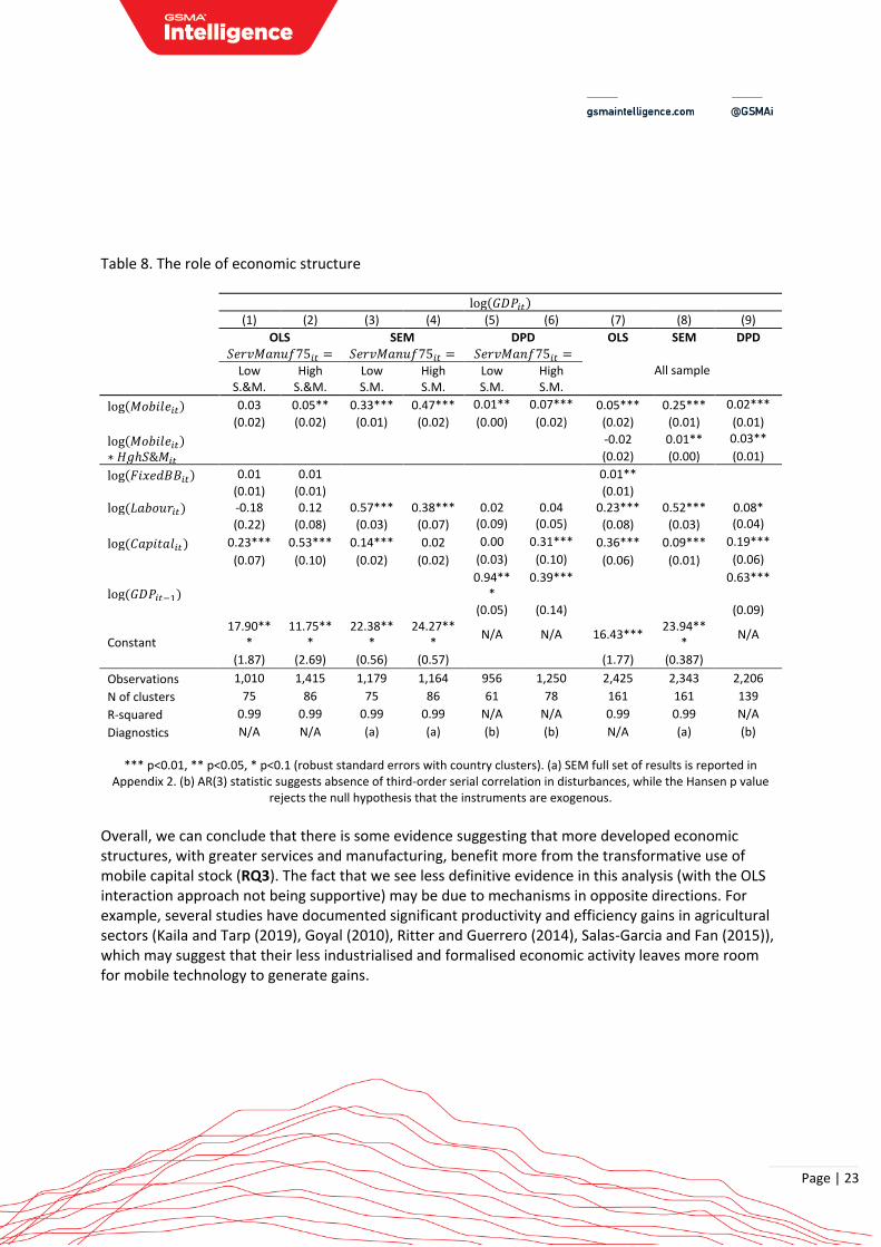
The literature suggests ICT’s impact differs depending on a country’s economic structure, given different complementarities between capital, labour and telecoms infrastructure. For example, fixed line and broadband studies have found service sectors benefit the most.26 More recently, the broadband literature shows stronger impacts in technology-intensive, scientific and technical sectors (Atasoy (2013), Kolko (2012), McCoy et al. (2017)); in banking, trade, construction and health (Nadiri and Nandi (2018)); or, in rural areas, the hospitality sector (Canzian et al. (2015)). These differences in aggregate impacts, meanwhile, have been less researched with regards to mobile technology. To address complementarities of mobile technology’s impact with economic structure, Table 8 shows regressions for the “High services & manufacturing” and “Low services & manufacturing” subsamples (based on the median of 75% of employment in these sectors). These cuts provide evidence that countries with more service and manufacturing activity enjoy stronger mobile impacts (columns 1–6 in Table 8). In fact, the OLS analysis suggests that this is a requirement for positive benefits to take place, while SEM and DPD predict approximately 1.4 to 7 times more gains in countries with a more advanced economic structure. The interaction approach – where mobile is interacted with a dummy taking value 1 when a country has employment in services and manufacturing above the median (𝐻𝑖𝑔ℎ𝑆𝑀𝑖𝑡) – support the same finding in SEM and DPD, though the additional impact related to an advanced economic structure is insignificant with OLS (columns 7–9).

26 For example, retail trade (Cronin et al. 1993; Cieslik & Kanjewsk 2004) finance, insurance and real estate (Greenstein & Spiller, 1995).

Page | 23

Table 8. The role of economic structure


(1) (2) (3) (4) (5) (6) (7) (8) (9)

OLS SEM DPD OLS SEM DPD 𝑆𝑒𝑟𝑣𝑀𝑎𝑛𝑢𝑓75𝑖𝑡 = 𝑆𝑒𝑟𝑣𝑀𝑎𝑛𝑢𝑓75𝑖𝑡 = 𝑆𝑒𝑟𝑣𝑀𝑎𝑛𝑓75𝑖𝑡 =

All sample

Low S.&M.

High S.&M.

Low S.M.

High S.M.

Low S.M.

High S.M.

log(𝑀𝑜𝑏𝑖𝑙𝑒𝑖𝑡) 0.03 0.05** 0.33*** 0.47*** 0.01** 0.07*** 0.05*** 0.25*** 0.02***

(0.02) (0.02) (0.01) (0.02) (0.00) (0.02) (0.02) (0.01) (0.01)

log(𝑀𝑜𝑏𝑖𝑙𝑒𝑖𝑡)∗ 𝐻𝑔ℎ𝑆&𝑀𝑖𝑡

-0.02 0.01** 0.03**

(0.02) (0.00) (0.01)

log(𝐹𝑖𝑥𝑒𝑑𝐵𝐵𝑖𝑡) 0.01 0.01 0.01**

(0.01) (0.01) (0.01)

log(𝐿𝑎𝑏𝑜𝑢𝑟𝑖𝑡) -0.18 0.12 0.57*** 0.38*** 0.02 0.04 0.23*** 0.52*** 0.08*

(0.22) (0.08) (0.03) (0.07) (0.09) (0.05) (0.08) (0.03) (0.04)

log(𝐶𝑎𝑝𝑖𝑡𝑎𝑙𝑖𝑡) 0.23*** 0.53*** 0.14*** 0.02 0.00 0.31*** 0.36*** 0.09*** 0.19***

(0.07) (0.10) (0.02) (0.02) (0.03) (0.10) (0.06) (0.01) (0.06)

log(𝐺𝐷𝑃𝑖𝑡−1)

0.94***

0.39***

0.63***

(0.05) (0.14) (0.09)

Constant 17.90**

* 11.75**

* 22.38**

* 24.27**

* N/A N/A 16.43***

23.94***

N/A

(1.87) (2.69) (0.56) (0.57) (1.77) (0.387)

Observations 1,010 1,415 1,179 1,164 956 1,250 2,425 2,343 2,206

N of clusters 75 86 75 86 61 78 161 161 139

R-squared 0.99 0.99 0.99 0.99 N/A N/A 0.99 0.99 N/A

Diagnostics N/A N/A (a) (a) (b) (b) N/A (a) (b)



Overall, we can conclude that there is some evidence suggesting that more developed economic structures, with greater services and manufacturing, benefit more from the transformative use of mobile capital stock (RQ3). The fact that we see less definitive evidence in this analysis (with the OLS interaction approach not being supportive) may be due to mechanisms in opposite directions. For example, several studies have documented significant productivity and efficiency gains in agricultural sectors (Kaila and Tarp (2019), Goyal (2010), Ritter and Guerrero (2014), Salas-Garcia and Fan (2015)), which may suggest that their less industrialised and formalised economic activity leaves more room for mobile technology to generate gains.

Page | 24

The role of income

The role of income is theoretically ambiguous. On the one hand, developing countries have labour and capital that tends to be less complementary with ICT infrastructure. On the other, developing countries have more limited fixed infrastructure deployment, meaning there is more room for mobile technology to drive productivity and efficiency gains.27 Some papers have found that mobile broadband and mobile in general have larger impacts in low-income countries (e.g. ITU (2018)). We also considered differences in returns to mobile technology depending on income levels, using both sample splits and interaction terms. We obtained mixed results, with diagnostics for SEM, DPD and IV approaches suggesting we could not draw conclusions from these analyses. We note that the studies showing higher impacts in developing countries seem to point that the fact these economies had poorer (fixed) communications infrastructure at the time of the arrival of mobile is a strong impact channel. That is, this lack of pre-existing infrastructure may have left more room for mobile to trigger stronger market efficiency and productivity improvements – with this more than offsetting the likely lower gains from lower levels of take-up (i.e. the role of nonlinearities), less education (i.e. the role of skills) and less services and manufacturing activity (i.e. the role of a complementary economic structure).

27 Lee et al. (2012) demonstrate that the impact of mobile telecommunications is stronger in developing countries with less developed wireline telecommunications infrastructure.

Page | 25

6. Conclusions The last two decades have seen much research devoted to understanding the economic impact of telecoms infrastructure – primarily operating through reductions in information, search and transaction costs and through being a complement or replacement of existing production inputs. However, while fixed communications and broadband have been extensively researched, the literature on mobile technology is more limited. Most studies have addressed the rollout of mobile until 2010, which is before the recent explosion in the use of mobile broadband (especially in developing countries). Only a recent wave of research has aimed to address the role of mobile broadband – but there still remains a number of research gaps. This study contributes to the existing body of literature in four ways. First, we analyse one of the most comprehensive panels in the recent literature, covering 160 countries from the early rollouts of 2G in 2000 to the 4G cycle in 2017. Second, importantly, this is a novel paper in unpicking the specific impacts of 2G, 3G and 4G technology, addressing whether there are additional impacts with newer infrastructure. Third, we evaluate heterogeneities in the macroeconomic impact of mobile, considering nonlinearities, skills and economic structure. Fourth, this paper simultaneously applies three separate methods to address endogeneity, including Structural Equations Models, Dynamic Panel Data and Instrumental Variable models. Firstly, we find that mobile technology was a significant driver of GDP in the 2000–2017 period. Specifically, our analysis has found that a 10% increase in the rate of mobile adoption increases GDP by 0.5–1.2%, with these effects remaining broadly stable over the period analysed. This is in line with impacts found in related literature, and provides further reassurance of the efficiency and productivity gains triggered by mobile technology. Our analysis has also revealed that these impacts materialise over and above the effect of fixed broadband, implying that countries that have fixed infrastructure in place can still benefit from further developing communications infrastructure through mobile. Secondly, we find that the rollout of subsequent 2G, 3G and 4G network technology has driven incremental impacts. Specifically, mobile’s baseline connectivity impact increases by about 15% when connections are upgraded to 3G. For connections upgrading form 2G to 4G, the impact increases by approximately 25%. Thirdly, we have noted three significant heterogeneities, pointing to mechanisms of impact and giving policymakers an understanding of how they can maximise the impact of mobile technology. The impact of mobile increases with adoption levels, suggesting network effects; countries with more skills enjoy greater impacts, suggesting complementarities with human capital accumulation; and we found some evidence of higher impact where services and manufacturing represent a greater share of economic activity, suggesting complementarities with capital and labour in these sectors.

Page | 26

Our findings point to at least three areas of further research. First, following our result of increased impacts with 2G, 3G and 4G, there is value in looking at other quality metrics with more granularity and variability, such as data speeds. This has started gaining traction in the literature, though primarily for developed countries (e.g. Ahlfeldt et al. (2016)). Second, further research is required to understand how and why impacts differ in developed and developing countries. Our heterogeneity analysis reveals some mechanisms, suggesting lower impacts in developing countries (i.e. take-up level, skills or economic structure) – however, empirical evidence tends to suggest greater impacts in developing economies. Having more evidence to understand why this is the case is required. Finally, as continued innovation takes place, particularly as 5G and IoT start to expand, further analysis is required to understand their economic impacts.

Page | 27

References Ahlfeldt, G., Koutroumpis, P., & Valletti, T. (2017). “Speed 2.0-Evaluating Access to Universal Digital

Highways”. Journal of the European Economic Association. ISSN 1542-4766. Aker, J. C. (2010). “Information from Markets Near and Far: Mobile Phones and Agricultural Markets in

Niger”. American Economic Journal: Applied Economics, 2(3), pp. 46–59. Arvin, B. M., & Pradhan, R. P. (2014). “Broadband Penetration and Economic Growth Nexus: Evidence

from Cross-country Panel Data”. Applied Economics, 46(35), pp. 4360-4369. Atasoy, H. (2013). “The Effects of Broadband Internet Expansion on Labor Market Outcomes”. Industrial

& Labor Relations Review, 66(2), pp. 315–345. Bertschek, I., Briglauer, W., Hüschelrath, K., Kauf, B., Niebel, T. (2017). “The Economic Impacts of

Telecommunications Networks and Broadband Internet: A Survey”. ZEW Center for European Economic Research, Discussion Paper No. 16-056

Canzian, G., Poy, S., & Schüller, S. (2015). “Broadband Diffusion and Firm Performance in Rural Areas: Quasi-Experimental Evidence”. IZA Discussion Papers no. 9429.

Canzian, G., Poy, S., & Schüller, S. (2015). “Broadband Diffusion and Firm Performance in Rural Areas: Quasi-Experimental Evidence”. IZA Discussion Papers no. 9429.

Cieślik, A., & Kaniewsk, M. (2004). “Telecommunications Infrastructure and Regional Economic Development: The Case of Poland”. Regional Studies” 38(6), pp. 713–725.

Cronin, F. J., Colleran, E. K., Herbert, P. L., & Lewitzky, S. (1993). “Telecommunications and Growth: The Contribution of Telecommunications Infrastructure Investment to Aggregate and Sectoral Productivity”. Telecommunications Policy, 17(9), pp. 677–690.

Czernich, N., Falck, O., Kretschmer, T., & Woessmann, L. (2011). “Broadband Infrastructure and Economic Growth”. The Economic Journal, 121(552), pp. 505–532.

Czernich, N. (2014). “Does Broadband Internet Reduce the Unemployment Rate? Evidence for Germany”. Information Economics and Policy, 29, pp. 32–45.

Edquist, H., Goodridge, P., Haskel, J., Li, X. & Lindquist, E. (2018). “How important Are Mobile Broadband Networks for the Global Economic Development?”. Information Economics and Policy, 45, pp. 16–29.

Forero, M. D. P. B. (2013). “Mobile Communication Networks and Internet Technologies as Drivers of Technical Efficiency Improvement”. Information Economics and Policy, 25(3), pp. 126–141.

Forman, C., A. Goldfarb & Greenstein, S. (2012). “The Internet and Local Wages: A Puzzle”. American Economic Review, 102, 556-575.

Giday, G. (2019). “Information communications technology and economic growth in Sub-Saharan Africa: A panel data approach”. Telecommunications Policy, 43(1), pp. 88–99.

Gillwald, A. & Mothobi, O. (2018). “After access 2018. A demand-side view of mobile internet from 10 African countries”. Research ICT Africa.

Goyal, A. 2010. “Information, direct access to farmers, and rural market performance in central India.” American Economic Journal: Applied Economics, 2(3): 22–45.

Page | 28

Greenstein, S. M., & Spiller, P. T. (1995). “Modern Telecommunications Infrastructure and Economic Activity: An Empirical Investigation. Industrial and Corporate Change”, 4(4), pp. 647–665.

Gruber, H., Hätönen, J., & Koutroumpis, P. (2014). “Broadband Access in the EU: An Assessment of Future Economic Benefits”. Telecommunications Policy, 38(11), pp. 1046–1058.

GSMA (2018). “Assessing the impact of market structure on innovation and quality in Central America”. Available at <https://www.gsma.com/publicpolicy/resources/driving-mobile-broadband-in-central-america>.

Houngbonon, G.V. & Jeanjean, F. (2016). “What level of competition intensity maximises investment in the wireless industry?". Telecommunications Policy, 40(8), 774–790.

HSBC (2015). “Supersonic: European telecoms mergers will boost capex, driving prices lower and speeds higher".

ITU. (2018). “The economic contribution of broadband, digitization and ICT regulation”. Expert reports series. Report authored by Katz, R. & Callorda, F.

Kaila, Heidi and Finn Tarp. 2019. “Can the Internet Improve Agricultural Production? Evidence from Viet Nam”.

Kolko, J. (2012). Broadband and Local Growth. Journal of Urban Economics, 71(1), pp. 100–113. Koutroumpis, P. (2009). “The Economic Impact of Broadband on Growth: A Simultaneous Approach”.

Telecommunications Policy, 33(9), pp. 471–485. Koutroumpis, P. (2016). “The mobile broadband premium in the Thai economy”. Unpublished. Koutroumpis, P. (2018). “The economic impact of broadband: evidence from OECD countries”. Report

prepared for Ofcom. Lam, P. L., & Shiu, A. (2010). “Economic Growth, Telecommunications Development and Productivity

Growth of the Telecommunications Sector: Evidence Around the World”. Telecommunications Policy, 34(4), pp. 185–199.

Lee, S. H., Levendis, J., & Gutierrez, L. (2012). “Telecommunications and Economic Growth: An Empirical Analysis of Sub-Saharan Africa”. Applied Economics, 44(4), pp. 461–469.

Mack, E., & Faggian, A. (2013). “Productivity and Broadband The Human Factor”. International Regional Science Review, 36(3), pp. 392–423.

McCoy, D., Lyons, S., Morgenroth, E., Palcic, D. & Allen, L. (2017. “The impact of broadband and other infrastructure on the location of new business establishments”. Grantham Research Institute on Climate Change and the Enviornment Working Paper No. 282.

Muto, M., & Yamano, T. (2009). “The Impact of Mobile Phone Coverage Expansion on Market Participation: Panel Data Evidence from Uganda”. World Development", 37(12), pp. 1887–1896.

Ritter, P. and M. Guerrero. 2014. “The Effect of the Internet and Cell Phones on Employment and Agricultural Production in Rural Villages in Peru.” Working paper, University of Piura, Piura, Peru.

Röller, L. H., & Waverman, L. (2001). “Telecommunications Infrastructure and Economic Development: A Simultaneous Approach”. American Economic Review, 91(4), pp. 909–923.

Thompson, H. G., & Garbacz, C. (2011). “Economic Impacts of Mobile Versus Fixed Broadband. Telecommunications Policy”, 35(11), pp. 999–1009.

https://www.gsma.com/publicpolicy/resources/driving-mobile-broadband-in-central-america

https://www.gsma.com/publicpolicy/resources/driving-mobile-broadband-in-central-america

Page | 29

Ward, M. R., & Zheng, S. (2016). “Mobile Telecommunications Service and Economic Growth: Evidence from China”. Telecommunications Policy, 40(2-3), pp. 89–101.

Waverman, L., Meschi, M., & Fuss, M. (2005). “The Impact of Telecoms on Economic Growth in Developing Countries”. Vodafone Policy Paper Series, 2, pp. 10–23.

Whitacre, B., Gallardo, R., & Strover, S. (2014). “Broadband’s Contribution to Economic Growth in Rural Areas: Moving Towards a Causal Relationship”. Telecommunications Policy, 38(11), pp. 1011–1023.

Page | 30

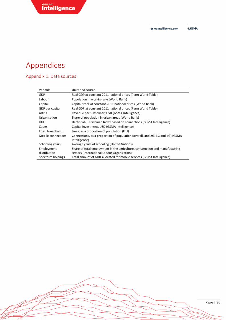
Appendices Appendix 1. Data sources

Variable Units and source

GDP Real GDP at constant 2011 national prices (Penn World Table)

Labour Population in working age (World Bank)

Capital Capital stock at constant 2011 national prices (World Bank)

GDP per capita Real GDP at constant 2011 national prices (Penn World Table)

ARPU Revenue per subscriber, USD (GSMA Intelligence)

Urbanisation Share of population in urban areas (World Bank)

HHI Herfindahl-Hirschman Index based on connections (GSMA Intelligence)

Capex Capital investment, USD (GSMA Intelligence)

Fixed broadband Lines, as a proportion of population (ITU)

Mobile connections Connections, as a proportion of population (overall, and 2G, 3G and 4G) (GSMA Intelligence)

Schooling years Average years of schooling (United Nations)

Employment distribution

Share of total employment in the agriculture, construction and manufacturing sectors (International Labour Organization)

Spectrum holdings Total amount of MHz allocated for mobile services (GSMA Intelligence)

Page | 31

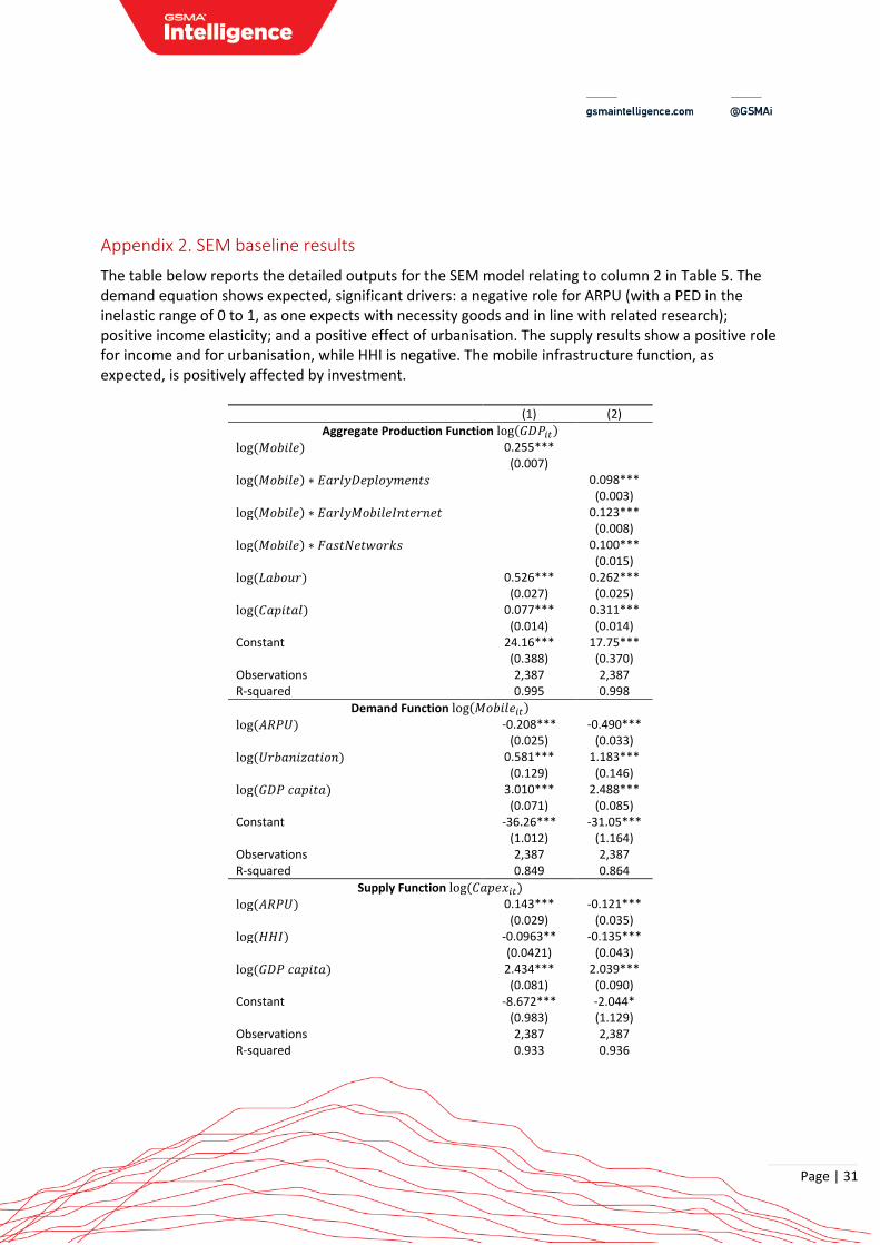
Appendix 2. SEM baseline results

The table below reports the detailed outputs for the SEM model relating to column 2 in Table 5. The demand equation shows expected, significant drivers: a negative role for ARPU (with a PED in the inelastic range of 0 to 1, as one expects with necessity goods and in line with related research); positive income elasticity; and a positive effect of urbanisation. The supply results show a positive role for income and for urbanisation, while HHI is negative. The mobile infrastructure function, as expected, is positively affected by investment.

(1) (2)

Aggregate Production Function log(𝐺𝐷𝑃𝑖𝑡)

log (𝑀𝑜𝑏𝑖𝑙𝑒) 0.255*** (0.007) log(𝑀𝑜𝑏𝑖𝑙𝑒) ∗ 𝐸𝑎𝑟𝑙𝑦𝐷𝑒𝑝𝑙𝑜𝑦𝑚𝑒𝑛𝑡𝑠 0.098***

(0.003)

log(𝑀𝑜𝑏𝑖𝑙𝑒) ∗ 𝐸𝑎𝑟𝑙𝑦𝑀𝑜𝑏𝑖𝑙𝑒𝐼𝑛𝑡𝑒𝑟𝑛𝑒𝑡 0.123***

(0.008)

log(𝑀𝑜𝑏𝑖𝑙𝑒) ∗ 𝐹𝑎𝑠𝑡𝑁𝑒𝑡𝑤𝑜𝑟𝑘𝑠 0.100***

(0.015)

log (𝐿𝑎𝑏𝑜𝑢𝑟) 0.526*** 0.262*** (0.027) (0.025)

log (𝐶𝑎𝑝𝑖𝑡𝑎𝑙) 0.077*** 0.311*** (0.014) (0.014) Constant 24.16*** 17.75***

(0.388) (0.370) Observations 2,387 2,387 R-squared 0.995 0.998

Demand Function log(𝑀𝑜𝑏𝑖𝑙𝑒𝑖𝑡)

log (𝐴𝑅𝑃𝑈) -0.208*** -0.490***

(0.025) (0.033)

log (𝑈𝑟𝑏𝑎𝑛𝑖𝑧𝑎𝑡𝑖𝑜𝑛) 0.581*** 1.183***

(0.129) (0.146)

log (𝐺𝐷𝑃 𝑐𝑎𝑝𝑖𝑡𝑎) 3.010*** 2.488***

(0.071) (0.085) Constant -36.26*** -31.05***


Supply Function log(𝐶𝑎𝑝𝑒𝑥𝑖𝑡)

log (𝐴𝑅𝑃𝑈) 0.143*** -0.121***

(0.029) (0.035)

log (𝐻𝐻𝐼) -0.0963** -0.135***

(0.0421) (0.043)

log (𝐺𝐷𝑃 𝑐𝑎𝑝𝑖𝑡𝑎) 2.434*** 2.039***

(0.081) (0.090) Constant -8.672*** -2.044*


Page | 32

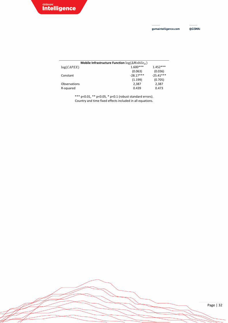
Mobile Infrastructure Function log(∆𝑀𝑜𝑏𝑖𝑙𝑒𝑖𝑡)

log (𝐶𝐴𝑃𝐸𝑋) 1.600*** 1.452***

(0.063) (0.036) Constant -28.17*** -25.41***


*** p<0.01, ** p<0.05, * p<0.1 (robust standard errors). Country and time fixed effects included in all equations.

Page | 33

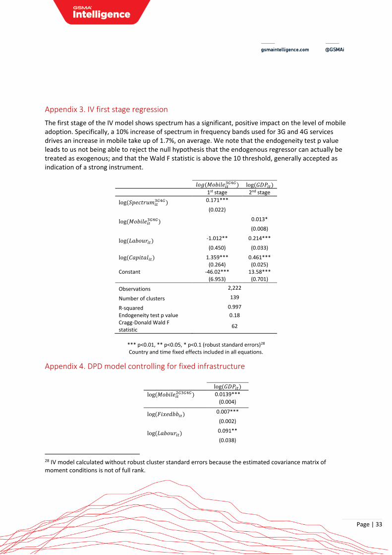
Appendix 3. IV first stage regression

The first stage of the IV model shows spectrum has a significant, positive impact on the level of mobile adoption. Specifically, a 10% increase of spectrum in frequency bands used for 3G and 4G services drives an increase in mobile take up of 1.7%, on average. We note that the endogeneity test p value leads to us not being able to reject the null hypothesis that the endogenous regressor can actually be treated as exogenous; and that the Wald F statistic is above the 10 threshold, generally accepted as indication of a strong instrument.

𝑙𝑜𝑔(𝑀𝑜𝑏𝑖𝑙𝑒𝑖𝑡3𝐺4𝐺) log(𝐺𝐷𝑃𝑖𝑡)

1st stage 2nd stage

log(𝑆𝑝𝑒𝑐𝑡𝑟𝑢𝑚𝑖𝑡3𝐺4𝐺) 0.171***

(0.022)

log(𝑀𝑜𝑏𝑖𝑙𝑒𝑖𝑡3𝐺4𝐺) 0.013*

(0.008)

log(𝐿𝑎𝑏𝑜𝑢𝑟𝑖𝑡) -1.012** 0.214***

(0.450) (0.033)

log(𝐶𝑎𝑝𝑖𝑡𝑎𝑙𝑖𝑡) 1.359*** 0.461***

(0.264) (0.025) Constant -46.02*** 13.58*** (6.953) (0.701)

Observations 2,222

Number of clusters 139

R-squared 0.997

Endogeneity test p value 0.18 Cragg-Donald Wald F statistic

62

*** p<0.01, ** p<0.05, * p<0.1 (robust standard errors)28 Country and time fixed effects included in all equations.

Appendix 4. DPD model controlling for fixed infrastructure


log(𝑀𝑜𝑏𝑖𝑙𝑒𝑖𝑡2𝐺3𝐺4𝐺) 0.0139***

(0.004)

log(𝐹𝑖𝑥𝑒𝑑𝑏𝑏𝑖𝑡) 0.007***

(0.002)

log(𝐿𝑎𝑏𝑜𝑢𝑟𝑖𝑡) 0.091**

(0.038)

28 IV model calculated without robust cluster standard errors because the estimated covariance matrix of moment conditions is not of full rank.

Page | 34

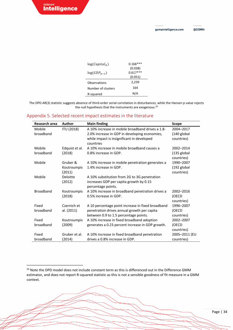
log(𝐶𝑎𝑝𝑖𝑡𝑎𝑙𝑖𝑡) 0.166***

(0.038)

log(𝐺𝐷𝑃𝑖𝑡−1) 0.617*** (0.051)

Observations 2,239

Number of clusters 164

R-squared N/A

The DPD AR(3) statistic suggests absence of third-order serial correlation in disturbances, while the Hansen p value rejects

the null hypothesis that the instruments are exogenous.29

Appendix 5. Selected recent impact estimates in the literature

Research area Author Main finding Scope

Mobile broadband

ITU (2018) A 10% increase in mobile broadband drives a 1.8-2.0% increase in GDP in developing economies, while impact is insignificant in developed countries

2004–2017 (140 global countries)

Mobile broadband

Edquist et al. (2018)

A 10% increase in mobile broadband causes a 0.8% increase in GDP.


Mobile Gruber & Koutroumpis (2011)

A 10% increase in mobile penetration generates a 1.4% increase in GDP.


Mobile Deloitte (2012)

A 10% substitution from 2G to 3G penetration increases GDP per capita growth by 0.15 percentage points.

Broadband Koutroumpis (2018)

A 10% increase in broadband penetration drives a 0.5% increase in GDP.

2002–2016 (OECD countries)

Fixed broadband

Czernich et al. (2011)

A 10 percentage point increase in fixed broadband penetration drives annual growth per capita between 0.9 to 1.5 percentage points.


Fixed broadband

Koutroumpis (2009)

A 10% increase in fixed broadband adoption generates a 0.23 percent increase in GDP growth.


Fixed broadband

Gruber et al. (2014)

A 10% increase in fixed broadband penetration drives a 0.8% increase in GDP.

2005–2011 (EU countries)

29 Note the DPD model does not include constant term as this is differenced out in the Difference GMM estimator, and does not report R-squared statistic as this is not a sensible goodness of fit measure in a GMM context.

GSMA Head OfficeFloor 2The Walbrook Building25 WalbrookLondon EC4N 8AFUnited KingdomTel: +44 (0)20 7356 0600 Fax: +44 (0)20 7356 0601

Documents

Mobile technology: two decades driving economic growth