MOBILE ROBOT PATH PLANNING USING A … ROBOT PATH PLANNING USING A CONSUMER 3D SCANNER A ... the Sick LMS 291, ... and actual performance in mapping an environment for a robotic platform

MOBILE ROBOT PATH PLANNING USING A CONSUMER 3D SCANNER

A

PROJECT

Presented to the Faculty

of the University of Alaska Fairbanks

in Partial Fulfillment of the Requirements

for the Degree of

MASTERS OF SCIENCE

By

Brian Paden, B.S.

Fairbanks, Alaska

December 2013

v2.1

ii

iii

Abstract

LIDAR range sensors are an increasingly popular sensing device for robotic systems due to their

accuracy and performance. Recent advances in consumer electronics have created hardware that is

inexpensive enough to be within the grasp of research projects without large budgets. This paper

compares the Kinect and a popular consumer LIDAR, the Sick LMS 291, in both their theoretical

and actual performance in mapping an environment for a robotic platform. In addition a new

algorithm for converting point cloud data to heightmaps is introduced and compared to known

alternatives. Point cloud and heightmap data formats are evaluated in terms of their real time

performance and design considerations.

Keywords: LIDAR, Kinect, point cloud, heightmap, Sick LMS 291

iv

v

Acknowledgments

I would like to express the deepest appreciation to my advisor Dr. Lawlor, who has always been

willing to help in any way possible with my projects; whether that be troubleshooting code, brain-

storming ideas or helping write a last minute grant proposal. Without your help this thesis (and

my masters) would not have happened.

Thank you to my committee members, Dr. Nance and Dr. Hartman for all of your helpful

feedback and direction. Editing was made much simpler for your effort and I am grateful for the

help.

In addition I would like to thank: The Alaska Space Grant Program for the numerous grants and

financial support; Mike Comberiate for putting together the project that got me started working

with LIDAR and for believing I could manage a large team of interns; Matt Anctil for helping

me wrangle said large team of interns; Steven Kibler for providing wisdom and a calming effect;

Robert Parsons for imparting knowledge and sacrificing your lab so we could build robots; NASA

Robotics Academy for granting me the chance to come work at NASA Goddard for a summer

and work along side some of the most interesting and intelligent people I have ever met; UAF for

being a quality university that attracts curiously brilliant students and faculty; LATEX, LibFreeNect,

OpenGL, Ubuntu and all the other open source projects that saved me countless hours of writing

code myself; and lastly to all my friends and family, you who supported me throughout this entire

project have my thanks and gratitude forever.

vi

vii

Table of Contents

Title Page . . . . . . . . . . . . . . . . . . . . . . . . . . . . . . . . . . . . . . . . . . . i

Abstract . . . . . . . . . . . . . . . . . . . . . . . . . . . . . . . . . . . . . . . . . . . . i

Acknowledgments . . . . . . . . . . . . . . . . . . . . . . . . . . . . . . . . . . . . . . . iii

Table of Contents . . . . . . . . . . . . . . . . . . . . . . . . . . . . . . . . . . . . . . . v

List of Figures . . . . . . . . . . . . . . . . . . . . . . . . . . . . . . . . . . . . . . . . . viii

List of Tables . . . . . . . . . . . . . . . . . . . . . . . . . . . . . . . . . . . . . . . . . ix

List of Algorithms . . . . . . . . . . . . . . . . . . . . . . . . . . . . . . . . . . . . . . . x

1 Introduction . . . . . . . . . . . . . . . . . . . . . . . . . . . . . . . . . . . . . . . . 1

2 UAFBot . . . . . . . . . . . . . . . . . . . . . . . . . . . . . . . . . . . . . . . . . . . 5

2.1 Requirements . . . . . . . . . . . . . . . . . . . . . . . . . . . . . . . . . . . . . . . . 6

2.2 Design . . . . . . . . . . . . . . . . . . . . . . . . . . . . . . . . . . . . . . . . . . . . 7

2.3 Schedule . . . . . . . . . . . . . . . . . . . . . . . . . . . . . . . . . . . . . . . . . . . 12

2.4 UAFBot Results . . . . . . . . . . . . . . . . . . . . . . . . . . . . . . . . . . . . . . 15

2.5 Future Work . . . . . . . . . . . . . . . . . . . . . . . . . . . . . . . . . . . . . . . . 21

3 Implementation Risks . . . . . . . . . . . . . . . . . . . . . . . . . . . . . . . . . . 23

3.1 Hardware Related . . . . . . . . . . . . . . . . . . . . . . . . . . . . . . . . . . . . . 23

3.2 Line of Sight Obstructions . . . . . . . . . . . . . . . . . . . . . . . . . . . . . . . . . 24

3.3 Accuracy . . . . . . . . . . . . . . . . . . . . . . . . . . . . . . . . . . . . . . . . . . 24

3.4 Noise . . . . . . . . . . . . . . . . . . . . . . . . . . . . . . . . . . . . . . . . . . . . . 26

3.5 Discretized Data . . . . . . . . . . . . . . . . . . . . . . . . . . . . . . . . . . . . . . 27

3.6 Ghosts . . . . . . . . . . . . . . . . . . . . . . . . . . . . . . . . . . . . . . . . . . . . 29

viii

3.7 Sensor Orientation Concerns . . . . . . . . . . . . . . . . . . . . . . . . . . . . . . . 29

3.8 Aged Data Culling . . . . . . . . . . . . . . . . . . . . . . . . . . . . . . . . . . . . . 31

4 LIDAR . . . . . . . . . . . . . . . . . . . . . . . . . . . . . . . . . . . . . . . . . . . 35

4.1 Sick LMS 291 . . . . . . . . . . . . . . . . . . . . . . . . . . . . . . . . . . . . . . . . 36

4.2 Kinect . . . . . . . . . . . . . . . . . . . . . . . . . . . . . . . . . . . . . . . . . . . . 36

4.3 Comparison . . . . . . . . . . . . . . . . . . . . . . . . . . . . . . . . . . . . . . . . . 37

5 Kinect Project . . . . . . . . . . . . . . . . . . . . . . . . . . . . . . . . . . . . . . . 39

5.1 Requirements . . . . . . . . . . . . . . . . . . . . . . . . . . . . . . . . . . . . . . . . 39

5.2 Design . . . . . . . . . . . . . . . . . . . . . . . . . . . . . . . . . . . . . . . . . . . . 40

5.3 Schedule . . . . . . . . . . . . . . . . . . . . . . . . . . . . . . . . . . . . . . . . . . . 43

5.4 Kinect Project Results . . . . . . . . . . . . . . . . . . . . . . . . . . . . . . . . . . . 44

5.5 Future Work . . . . . . . . . . . . . . . . . . . . . . . . . . . . . . . . . . . . . . . . 47

6 Data Formats . . . . . . . . . . . . . . . . . . . . . . . . . . . . . . . . . . . . . . . . 49

6.1 Point Clouds . . . . . . . . . . . . . . . . . . . . . . . . . . . . . . . . . . . . . . . . 49

6.2 Heightmaps . . . . . . . . . . . . . . . . . . . . . . . . . . . . . . . . . . . . . . . . . 50

6.3 Converting Point Clouds to Heightmaps . . . . . . . . . . . . . . . . . . . . . . . . . 52

6.4 Naive Conversion . . . . . . . . . . . . . . . . . . . . . . . . . . . . . . . . . . . . . . 53

6.5 FORM Conversion . . . . . . . . . . . . . . . . . . . . . . . . . . . . . . . . . . . . . 54

7 Concluding Remarks . . . . . . . . . . . . . . . . . . . . . . . . . . . . . . . . . . . 57

References . . . . . . . . . . . . . . . . . . . . . . . . . . . . . . . . . . . . . . . . . . . 61

ix

List of Figures

1.1 UAFBot with scanner . . . . . . . . . . . . . . . . . . . . . . . . . . . . . . . . . . . 2

2.1 UAFBot project schedule . . . . . . . . . . . . . . . . . . . . . . . . . . . . . . . . . 16

3.1 Point cloud line of sight obstructions . . . . . . . . . . . . . . . . . . . . . . . . . . . 25

3.2 Visible banding of ranges in hallway scan . . . . . . . . . . . . . . . . . . . . . . . . 28

3.3 Scan showing ghost effect . . . . . . . . . . . . . . . . . . . . . . . . . . . . . . . . . 30

5.1 Kinect project schedule . . . . . . . . . . . . . . . . . . . . . . . . . . . . . . . . . . 45

6.1 Scan of outdoor environment with heightmap overlay . . . . . . . . . . . . . . . . . . 51

6.2 Obstacle with multiple valid heights . . . . . . . . . . . . . . . . . . . . . . . . . . . 53

x

List of Tables

2.1 UAFVision scan durations with measured values . . . . . . . . . . . . . . . . . . . . 15

4.1 Kinect vs Sick LMS 291 specifications . . . . . . . . . . . . . . . . . . . . . . . . . . 38

xi

List of Algorithms

1 PERT Time Estimation . . . . . . . . . . . . . . . . . . . . . . . . . . . . . . . . . . 13

2 Fixed life span time culling of points . . . . . . . . . . . . . . . . . . . . . . . . . . . 33

3 Converting raw Kinect data to meters (i, j, k)→ (x, y, z) . . . . . . . . . . . . . . . . 46

4 Time Weighting Function . . . . . . . . . . . . . . . . . . . . . . . . . . . . . . . . . 46

5 Image to Cartesian coordinate conversion . . . . . . . . . . . . . . . . . . . . . . . . 50

6 Naive Point Cloud conversion . . . . . . . . . . . . . . . . . . . . . . . . . . . . . . . 54

7 FORM Point Cloud conversion . . . . . . . . . . . . . . . . . . . . . . . . . . . . . . 55

xii

1

Chapter 1

Introduction

The high cost of hardware has always been one of the major limiting factors in the development of

robotic platforms. While the cost of computers has fallen over the years, sensors often remain at a

premium price. A new generation of consumer hardware is changing this by making range-finding

sensors available at prices never before seen.

A useful sensor in robotics is a range-sensing device, one of the more common forms being

LIDAR.[1] These have numerous advantages over standard vision systems in the robotics world.

The key advantage is that LIDAR range sensors tell you precisely how far obstacles are from the

sensor. Vision systems, primarily stereoscopic vision systems, can provide this information as well

but generally at a much higher computational cost. Stereo vision systems also have great difficulty

when looking at images with low texture, such as blank walls or water. LIDAR range sensors

have the advantages of high accuracy and fast processing time but typically are more expensive

sensors.[2]

The Microsoft Kinect 360 is a strong first step towards changing this; consumer grade electronics

are cheaper and much more readily available to the robotics researcher or hobbyist. The original

launch price of the Kinect was less than one-twentieth that of an industry standard LIDAR. This

drastic reduction in cost is not free, however, and it is a key component of this project to demonstrate

the differences and limitations when comparing the two sensors.

The goal of this project was to create a software visualization environment that allowed for

experimentation and demonstrations of LIDAR like range sensing devices. Two sub-projects were

involved, the first being initial development and testing with a Sick LMS 291, the second utilizing

a Kinect. Although many of the concepts and visualization techniques were similar, the nature of

the hardware devices required different implementations. The Sick LMS 291 requires additional

hardware to create an image due to the fact that it only takes a one-dimensional scan line of the

environment. This necessitated building a rotating platform that could be accurately controlled to

2

create scans.

The first phase of the project, called UAFBot, took place at NASA Goddard during the summer

of 2009. My part of the project was to add a Sick LMS 291 atop a rotating platform to a new

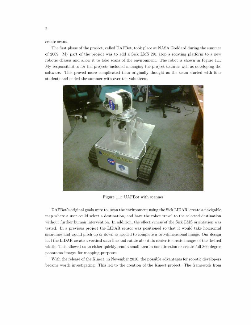
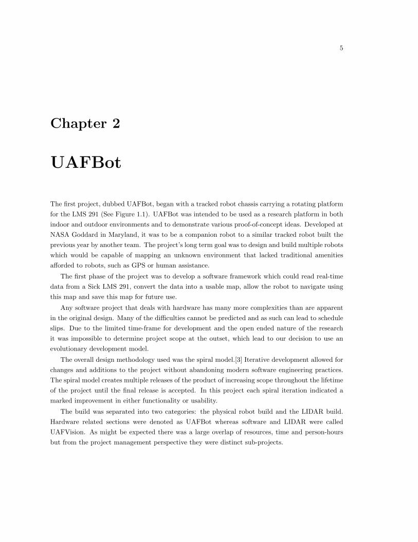
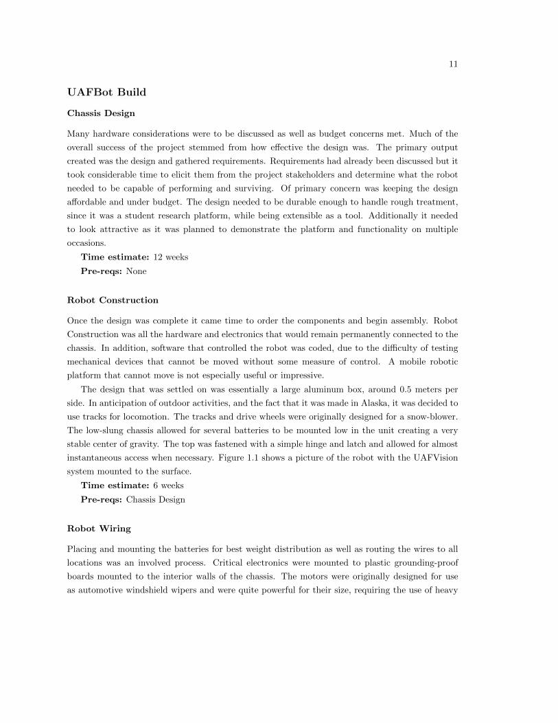
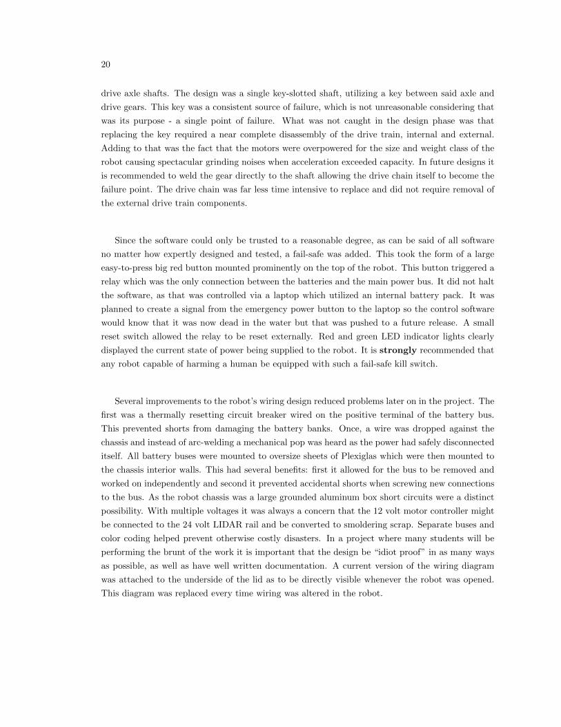
robotic chassis and allow it to take scans of the environment. The robot is shown in Figure 1.1.

My responsibilities for the projects included managing the project team as well as developing the

software. This proved more complicated than originally thought as the team started with four

students and ended the summer with over ten volunteers.

Figure 1.1: UAFBot with scanner

UAFBot’s original goals were to: scan the environment using the Sick LIDAR, create a navigable

map where a user could select a destination, and have the robot travel to the selected destination

without further human intervention. In addition, the effectiveness of the Sick LMS orientation was

tested. In a previous project the LIDAR sensor was positioned so that it would take horizontal

scan-lines and would pitch up or down as needed to complete a two-dimensional image. Our design

had the LIDAR create a vertical scan-line and rotate about its center to create images of the desired

width. This allowed us to either quickly scan a small area in one direction or create full 360 degree

panorama images for mapping purposes.

With the release of the Kinect, in November 2010, the possible advantages for robotic developers

became worth investigating. This led to the creation of the Kinect project. The framework from

3

UAFBot was reused to compare the differences between the Sick LMS 291 and the Kinect. By

utilizing the same framework it was possible to discern subtle variations in how the unique hardware

behaved. I was the sole student developer for the Kinect project and developed all the code used.

Creating a second project with a different range-finding sensor would allow for previous results

to be replicated as well as programming and algorithmic techniques to be refined. Of particular

interest was just how accurate the Kinect would be compared to the industry standard Sick LMS

291. The Kinect also provided more sensors than just range detecting. A color camera as well

as audio and accelerometer data are provided at 30 Hz. In particular the ability to check and

correct for orientation via accelerometer was of great interest. To create scans for testing with

UAFBot one always had to be careful to ensure the platform was on a level surface so that future

measurements would be accurate. With an accelerometer built into the hardware sensor this could

either be incorporated in real time or saved until later and the data reconciled.

4

5

Chapter 2

UAFBot

The first project, dubbed UAFBot, began with a tracked robot chassis carrying a rotating platform

for the LMS 291 (See Figure 1.1). UAFBot was intended to be used as a research platform in both

indoor and outdoor environments and to demonstrate various proof-of-concept ideas. Developed at

NASA Goddard in Maryland, it was to be a companion robot to a similar tracked robot built the

previous year by another team. The project’s long term goal was to design and build multiple robots

which would be capable of mapping an unknown environment that lacked traditional amenities

afforded to robots, such as GPS or human assistance.

The first phase of the project was to develop a software framework which could read real-time

data from a Sick LMS 291, convert the data into a usable map, allow the robot to navigate using

this map and save this map for future use.

Any software project that deals with hardware has many more complexities than are apparent

in the original design. Many of the difficulties cannot be predicted and as such can lead to schedule

slips. Due to the limited time-frame for development and the open ended nature of the research

it was impossible to determine project scope at the outset, which lead to our decision to use an

evolutionary development model.

The overall design methodology used was the spiral model.[3] Iterative development allowed for

changes and additions to the project without abandoning modern software engineering practices.

The spiral model creates multiple releases of the product of increasing scope throughout the lifetime

of the project until the final release is accepted. In this project each spiral iteration indicated a

marked improvement in either functionality or usability.

The build was separated into two categories: the physical robot build and the LIDAR build.

Hardware related sections were denoted as UAFBot whereas software and LIDAR were called

UAFVision. As might be expected there was a large overlap of resources, time and person-hours

but from the project management perspective they were distinct sub-projects.

6

2.1 Requirements

Functional requirements “...are statements of services the system should provide, how the system

should react to particular inputs and how the system should behave in particular situations.”[4]

Following are several functional requirements for both UAFBot and the UAFVision system.

1. UAFBot will be able to drive in outdoor terrain that a person could reasonably walk through.

2. UAFVision shall produce a 2D obstacle map of the robot’s local environment.

3. UAFVision will be able to reliably detect chair-sized obstacles at a range of 3 meters.

4. UAFVision will not attempt to drive through detected obstacles. If there is no way to reach

the goal, UAFVision shall stop.

Non-Functional Requirements fall under two categories: execution, which are observable at run

time; and evolution, which are embodied in the static structure of the program.[5]

The two main categories of non-functional requirements that are most relevant to this project

are performance and maintainability. Performance is concerned with meeting the real time demands

of both the hardware as well as rendering software and ensuring the user interface responded with

minimal delay. Maintainability forces the program to be well written and documented in such a

way that others will be able to use or expand upon it at a later date without contacting the original

developer.

Performance requirements are strict, as robots and hardware often fall under the category of

real-time systems. Commanding a powerful piece of metal to move about a room can have dire

consequences if a section of code takes too long to respond. Here are some of the more strict

performance requirements used to design UAFBot.

• PE-1: The software shall maintain exclusive control over UAFBot/UAFVision when operat-

ing.

• PE-2: The software shall read data from the LMS 291 at the hardware’s optimal rate, currently

known to be 30 Hz.

• PE-3: The software shall render updates to the rendering screen no slower than 15 Hz.

• PE-4: User input to the software shall be accepted and utilized no later than the next frame.

• PE-5: After 100 msec of no commands all hardware shall issue a hard stop command.

• PE-6: In the event of software failure all hardware shall immediately terminate action.

7

Maintenance was determined to be the other most important category of requirements for UAF-

Bot. In a project run by students one can never be certain who will return next year. Thus it was

necessary that all hardware and software was properly documented for future participants who may

have no contact with the original team. Additionally, experimental robots are often are stressed

beyond their limits and minimizing the difficulty of part replacement saves much stress and hard-

ship.

• MA-1: The code shall be written using known best standards and practices.

• MA-2: The project shall be documented in such a way that future maintenance is straight

forward to someone unfamiliar.

• MA-3: Code comments will document the “why,” not just what is. Intent and mind-set are

difficult for future developers to discover from the source code alone.

• MA-4: Hardware shall be “off the shelf” and avoid custom solutions whenever reasonable.

• MA-5: All electronic data (source code, documentation, etc.) shall be stored using version

control software.

2.2 Design

Following are the features that were planned for development of the hardware and software com-

ponents of UAFBot. Not all aspects of each feature were scheduled at project onset; additional

functionality was added as required. Nearly all features were planned in advance but several were

not identified until later in the build cycle and were added to later release stages, per the spiral

design methodology. Each stage was planned in detail towards the end of the previous stage and

stages were added until all required product features were incorporated.

UAFBot was a complicated project managed and operated by students with few faculty advisors.

It began with contact with NASA concerning whether it would be feasible to design less costly

robots that could map an unknown environment without the help of tools such as GPS that might

not be available. The project was conceived as a technical experiment in robotic sensing and

communication. The NASA element was created by Mike Comberiate, and the UAF students were

advised principally by Dr. Orion Lawlor with Robert Parsons advising and managing the lab where

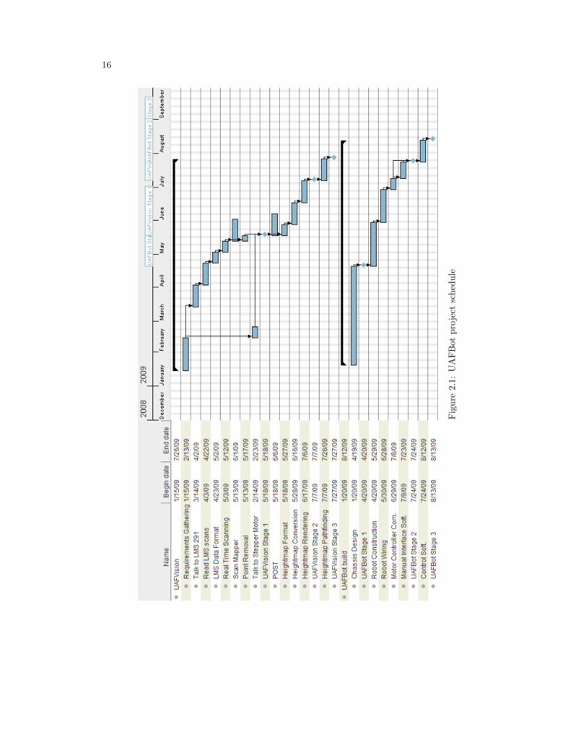
it was constructed. The entire UAFBot project Gantt chart can be found in Figure 2.1 along with

a more detailed project schedule.

8

UAFVision

UAFVision was primarily concerned in interacting with the LIDAR range sensor, gathering the

scans and creating maps from the data. A future project was to incorporate the maps and UAFBot

controls into a single functional robot. UAFVision Stage 1 consisted exclusively of requirement

gathering, design and research. It was at this time it was decided that the LIDAR range sensor was

to be oriented to take vertical scan-lines, as opposed to the horizontal lines the previous project

NASABot utilized; the primary reason being that the robot was intended as a mapping tool. Priority

was given to mapping versus mobility.

Requirements Gathering

Requirements gathering for UAFVision was a research phase where ideas were communicated be-

tween numerous project stakeholders and researchers. Due to the difficulty of planning discussions

between multiple geographic locations as well as the number of concepts involved this was allocated

four weeks.

Time estimate: 4 weeks

Pre-reqs: None

Talk to LMS 291

Communicating with the Sick LMS 291 required a serial connection and thus required familiarity

with that topic before the LIDAR could be accessed. The device was well used by researchers and

several tutorials were available which softened the learning curve significantly.


Pre-reqs: Requirements Gathering

Read LMS Scans

The LMS 291 communicates in binary data using a proprietary telegram format. Converting binary

packed data to floating point is fraught with subtle errors and extensive validation was necessary

to ensure correct values every time.


Pre-reqs: Talk to LMS 291

LMS Data Format

This further enhanced the capabilities of utilizing the scan-lines from the LIDAR. Much error

checking needed to be done converting packed binary data into more user friendly formats.


9

Pre-reqs: Read LMS Scans

Real Time Scanning

This feature involved improving performance and implementations of the software so it was capable

of receiving data at the same rate as the LIDAR sends it. Data not handled in time is lost and it

was important that this level of performance be achieved early in the project.


Pre-reqs: LMS Data Format

Scan Mapper

Scan Mapper took data streams once they had been read in from the LIDAR, converted the coor-

dinate system and rendered it to a GUI program, creating a significant improvement for debugging

and demonstration purposes. Scan Mapper was intended as a debugging and early visualization

tool at this stage, not for public demonstration.


Pre-reqs: Real Time Scanning

Point Removal

Point removal included handling cases where bad data was sent from the LIDAR. Care was taken

to avoid including this in samples. Data that could not be repaired was discarded and requested

again.

Time estimate: 1 week

Pre-reqs: Real Time Scanning

Talk to Stepper Motor

The stepper motor also utilized a serial port which allowed for library sharing between the LIDAR

and motor. It still possessed a unique communication protocol. The stepper motor did not require

a checksum for each communication packet, unlike the LMS 291.

Time estimate: 1.5 weeks

Pre-reqs: Requirements Gathering

POST

The POST (Power On Self Test) represented a complicated testing of the hardware on startup.

It was also essential before the hardware could perform normal operation. The basic procedure

connected to the LIDAR and stepper motor, took a simple scan from the LIDAR and moved the

10

stepper motor into position to begin scanning. Any failure in the steps alerted the software and

user. In most cases human intervention was necessary to fix the problem.


Pre-reqs: Real Time Scanning, Talk to Stepper Motor

Heightmap Format

This dealt with how to store and manipulate heightmap data. An extensive API was necessary as

it was the core of the mapping efforts. Data access was designed to be quick for random-access as

well as for looping across the entire data set.


Pre-reqs: POST

Heightmap Conversion

Converting point clouds to heightmaps was more complicated than it first appeared. Edge cases

must be handled properly and performance needs met. One such case is how to handle points that

land exactly on a border between cells. By default the point is added to a single cell instead of all

adjacent cells.


Pre-reqs: Heightmap Format

Heightmap Rendering

The heightmap rendering was pivotal for both debugging and demonstrating the project. This

software was the interface the client used to view the scanning and mapping results. Therefore

considerable time was allocated to ensuring it was visually appealing as well as free of major

defects.


Pre-reqs: Heightmap Conversion

Heightmap Path Finding

This module determined how to map a route given the robot specifications and a heightmap. A*

(pronounced A-star) was used on a saved scan as a proof-of-concept. The main problem of interest

was how to allow slope to affect pathfinding solutions.


Pre-reqs: Heightmap Rendering

11

UAFBot Build

Chassis Design

Many hardware considerations were to be discussed as well as budget concerns met. Much of the

overall success of the project stemmed from how effective the design was. The primary output

created was the design and gathered requirements. Requirements had already been discussed but it

took considerable time to elicit them from the project stakeholders and determine what the robot

needed to be capable of performing and surviving. Of primary concern was keeping the design

affordable and under budget. The design needed to be durable enough to handle rough treatment,

since it was a student research platform, while being extensible as a tool. Additionally it needed

to look attractive as it was planned to demonstrate the platform and functionality on multiple

occasions.


Pre-reqs: None

Robot Construction

Once the design was complete it came time to order the components and begin assembly. Robot

Construction was all the hardware and electronics that would remain permanently connected to the

chassis. In addition, software that controlled the robot was coded, due to the difficulty of testing

mechanical devices that cannot be moved without some measure of control. A mobile robotic

platform that cannot move is not especially useful or impressive.

The design that was settled on was essentially a large aluminum box, around 0.5 meters per

side. In anticipation of outdoor activities, and the fact that it was made in Alaska, it was decided to

use tracks for locomotion. The tracks and drive wheels were originally designed for a snow-blower.

The low-slung chassis allowed for several batteries to be mounted low in the unit creating a very

stable center of gravity. The top was fastened with a simple hinge and latch and allowed for almost

instantaneous access when necessary. Figure 1.1 shows a picture of the robot with the UAFVision

system mounted to the surface.


Pre-reqs: Chassis Design

Robot Wiring

Placing and mounting the batteries for best weight distribution as well as routing the wires to all

locations was an involved process. Critical electronics were mounted to plastic grounding-proof

boards mounted to the interior walls of the chassis. The motors were originally designed for use

as automotive windshield wipers and were quite powerful for their size, requiring the use of heavy

12

gauge wire to handle the current draw.


Pre-reqs: Robot Construction

Motor Controller Communication

Communicating with the motor controller required an additional serial device protocol. This fea-

ture also had strict real-time requirements as any delay could cause accidents damaging people or

property.


Pre-reqs: Robot Wiring

Manual Interface Software

Manual control of the robot was desirable for transportation as well as for testing of the mechanics.

Software was written to interface with a USB joystick controller for ease of use. This allowed fine

manual control of the robot for maneuvering as well as transportation as it weighs well over 30 kg

with full payload.


Pre-reqs: Motor Controller Communication

Control Software

This included software API’s that could control the robot either remotely or from more advanced

on-board AI programs. All access to hardware passed through this software, no direct connections

are allowed.


Pre-reqs: Manual Interface Software

2.3 Schedule

When one is designing the schedule of a project the design methodology plays a large part. In the

well known Waterfall methodology all target goals are set at the beginning of the project. Agile

development is the polar opposite, where time and resource estimations are made at the beginning

of each individual task. As mentioned, the Spiral method was used for UAFBot, which divided the

project into several stages. Each stage had a set feature list, requirements to meet and an estimated

deadline.

Many methods exist to estimate the time that will be involved in developing software. These

can not guarantee accurate information, only help the estimator create better cost measurements.

13

Industry professionals tend to agree that software estimation is as much an art as it is a science

and relies heavily on the judgment of the person performing the estimation.[6]

The PERT method (Program Evaluation and Review Technique) was used to create estimates of

both the hardware and software schedules.[6] Hardware time estimates were created with help from

team members who had more experience with the areas outside my expertise. Software estimates

were created based on my experience and proficiency level as I was the primary developer. PERT

combines worst case, best case and most likely case in a weighted average, the formula is shown in

Algorithm 1.

Algorithm 1 PERT Time Estimation

W is the worst case estimateL is the most likely estimateB is the best case estimatePERT ← (W + 4 ∗ L+B)/6

An important consideration when creating time estimates for projects is what units to use. Most

commonly used are hours for small tasks and days for standard sized ones. One subtle issue with

using smaller units is that there exists an implied precision. Stating the project will take 90 days

sounds much more precise than saying three months. If the task is scheduled for three months and

goes over another two weeks that doesn’t seem as inaccurate as going from 90 to 104 days, when

it is of course the same duration. It is for this reason that the default unit of time for scheduling

was chosen to be weeks, assuming four to five work days per week on average. No features were

estimated to take fewer than one week and the longest duration was planned at twelve.

UAFVision

UAFVision’s schedule was broken up into three major milestones, called stages. Each stage repre-

sented a significant addition of functionality to the project.

Stage 1

Stage 1 of UAFVision represented the first usable phase of development. Requirements and design

were completed for the hardware and software components. All unique elements of hardware were

functional and able to communicate with their respective control software.


Stage 2

Stage 2 added heightmap functionality to the existing scanning abilities. This included every aspect

from converting the point cloud to a heightmap and rendering to a screen, as well as storing the

14

data in a computer friendly format. This was the majority of requested features and functionality

for the current goals of the overarching project. It was determined that accomplishing this would

meet the current project goals for the summer internship.


Stage 3

Stage 3 expanded on the heightmap functionality by adding path finding and navigation. The

most realistic expectation was that it would be possible to create routes based on scans. It seemed

unlikely that full autonomous navigation would be connected to the path-finding during this phase

of research.


UAFBot

Stage 1

The entirety of Stage 1 for UAFBot consisted of determining project scope, requirement elicitation

and designing and engineering the robotic platform. Many stake holders were involved and cross-

communication was key. Engineering is the fine art of balancing what users would like to have

done, what needs to be done and what can actually be done. The chassis had to be strong enough

to support the payload, have enough battery capacity to be useful and be light enough to be

transported without a forklift.


Stage 2

Stage 2 began construction of the robot. The first step was procuring all necessary materials as

well as a work space to build the robot. Assembling all the components into the correct shape

does not make a robot, however. The electrical system was quite involved for a basic two-tracked

design. Included in wiring was the electronic control system for the motors and motor controller.

Completion marked the end of the build and a fully functional, albeit brainless, robot was built.


Stage 3

UAFBot Stage 3 was the first that did not involve any hardware. It was focused solely on developing

software to control the robot. This included communicating between the motor controller and robot

mounted computer as well as creating a human interface. A USB joystick was selected due to the

15

intuitiveness and simplicity of control. A software framework was developed and documented as

well to enable future control aspects.


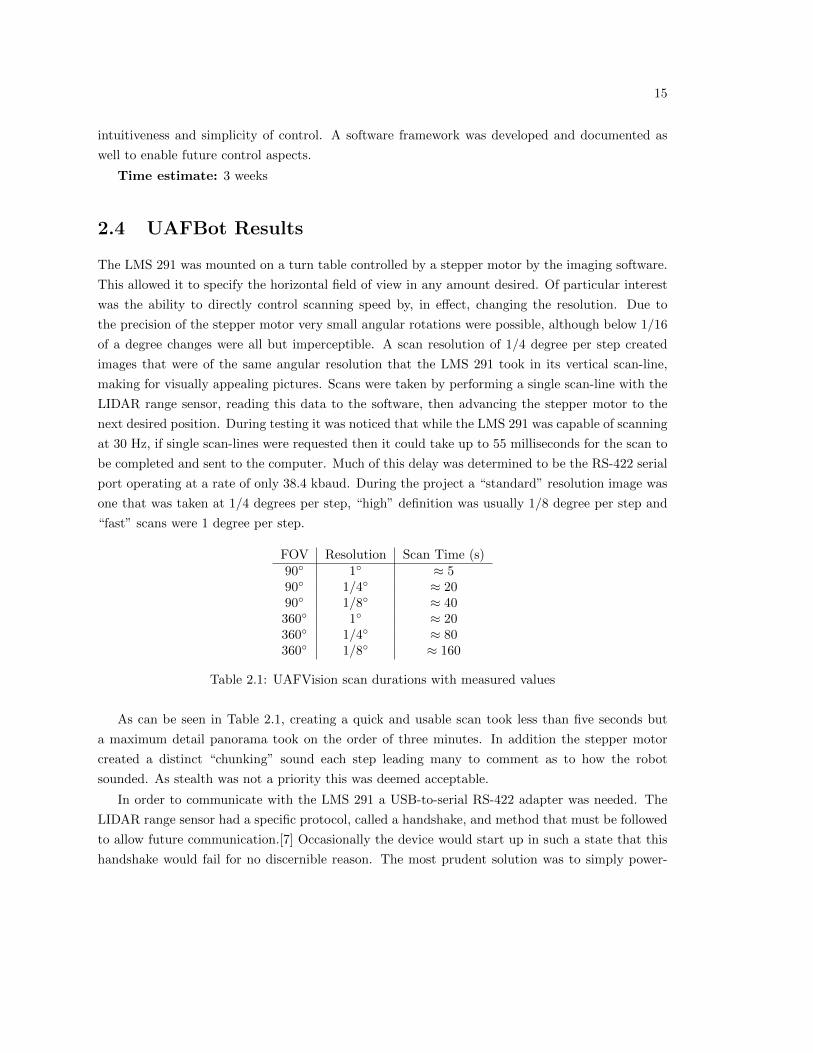
2.4 UAFBot Results

The LMS 291 was mounted on a turn table controlled by a stepper motor by the imaging software.

This allowed it to specify the horizontal field of view in any amount desired. Of particular interest

was the ability to directly control scanning speed by, in effect, changing the resolution. Due to

the precision of the stepper motor very small angular rotations were possible, although below 1/16

of a degree changes were all but imperceptible. A scan resolution of 1/4 degree per step created

images that were of the same angular resolution that the LMS 291 took in its vertical scan-line,

making for visually appealing pictures. Scans were taken by performing a single scan-line with the

LIDAR range sensor, reading this data to the software, then advancing the stepper motor to the

next desired position. During testing it was noticed that while the LMS 291 was capable of scanning

at 30 Hz, if single scan-lines were requested then it could take up to 55 milliseconds for the scan to

be completed and sent to the computer. Much of this delay was determined to be the RS-422 serial

port operating at a rate of only 38.4 kbaud. During the project a “standard” resolution image was

one that was taken at 1/4 degrees per step, “high” definition was usually 1/8 degree per step and

“fast” scans were 1 degree per step.

FOV Resolution Scan Time (s)90◦ 1◦ ≈ 590◦ 1/4◦ ≈ 2090◦ 1/8◦ ≈ 40360◦ 1◦ ≈ 20360◦ 1/4◦ ≈ 80360◦ 1/8◦ ≈ 160

Table 2.1: UAFVision scan durations with measured values

As can be seen in Table 2.1, creating a quick and usable scan took less than five seconds but

a maximum detail panorama took on the order of three minutes. In addition the stepper motor

created a distinct “chunking” sound each step leading many to comment as to how the robot

sounded. As stealth was not a priority this was deemed acceptable.

In order to communicate with the LMS 291 a USB-to-serial RS-422 adapter was needed. The

LIDAR range sensor had a specific protocol, called a handshake, and method that must be followed

to allow future communication.[7] Occasionally the device would start up in such a state that this

handshake would fail for no discernible reason. The most prudent solution was to simply power-

16

Fig

ure

2.1

:U

AF

Bot

pro

ject

sch

edu

le

17

cycle the LIDAR and attempt again. Even with documentation it took a sizable amount of time to

create software that would reliably open correspondence with the LMS 291. The protocol is fairly

standard by serial port methods: a message is sent by the computer and the LIDAR range sensor

responds in kind. Regular “keep alive” messages are sent from the LIDAR devices well if no other

messages are sent. Checksums are also used to verify the integrity of the connection.

Even after considerable time with the LIDAR, converting ranges in an array into understandable

data proved difficult. Early in UAFVision Stage 1 a graphical program was developed. Originally

a single line was rendered as the LMS 291 only outputted two dimensions of data. This allowed

basic orientation, and for us to discover that the way the LIDAR range sensor was mounted to the

platform was upside-down according to the scan-lines. This was solved by a simple fix in software

but made for very confusing images until it was discovered. The scanning software was designed

to scan an area and then present the data as a range image to a graphical user interface using

OpenGL. At Stage 1 it was more prudent to render any image at all rather than deal with the

complexities of adding new points as they were scanned. OpenGL is far more optimized to handle

polygons, most commonly triangles, then it is points. As such, on a high detail scan points that were

actually scanned would not render to the user. It was later determined that this was a limitation

of vertex buffer objects in OpenGL. This can be solved by breaking up points into multiple buffers.

Overcoming this would have involved a significant rewrite of the rendering code and was postponed

to a future development stage.

An important addition to UAFVision Stage 2 was a power on self test (POST) routine. With

all hardware it is important to verify that no errors have occurred before any attempt to utilize

them is made. Performing a POST is an industry standard method to run through a diagnostic

routine every power on and ensure everything is properly configured and responsive.

The UAFVision POST method followed this procedure:

1. Power is supplied to the UAFVision hardware

2. Wait until the LMS 291 indicates ready status via green LED

3. Initialize control software

4. Software connects to LMS 291 via handshake

5. Software reads single scan from LIDAR

6. Software connects to stepper motor

7. Stepper motor rotates 5◦ counter-clockwise

8. Stepper motor rotates clockwise until sensor indicating zero position is triggered

9. Now ready to receive instructions for scans

18

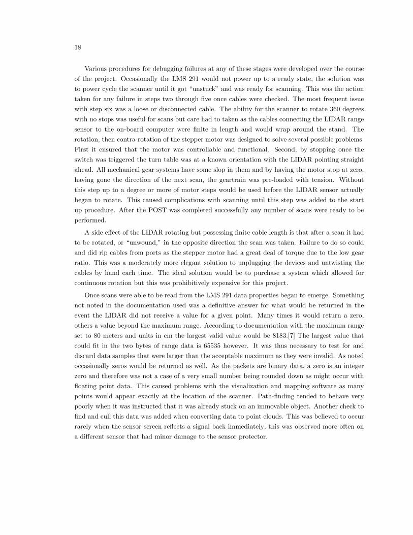
Various procedures for debugging failures at any of these stages were developed over the course

of the project. Occasionally the LMS 291 would not power up to a ready state, the solution was

to power cycle the scanner until it got “unstuck” and was ready for scanning. This was the action

taken for any failure in steps two through five once cables were checked. The most frequent issue

with step six was a loose or disconnected cable. The ability for the scanner to rotate 360 degrees

with no stops was useful for scans but care had to taken as the cables connecting the LIDAR range

sensor to the on-board computer were finite in length and would wrap around the stand. The

rotation, then contra-rotation of the stepper motor was designed to solve several possible problems.

First it ensured that the motor was controllable and functional. Second, by stopping once the

switch was triggered the turn table was at a known orientation with the LIDAR pointing straight

ahead. All mechanical gear systems have some slop in them and by having the motor stop at zero,

having gone the direction of the next scan, the geartrain was pre-loaded with tension. Without

this step up to a degree or more of motor steps would be used before the LIDAR sensor actually

began to rotate. This caused complications with scanning until this step was added to the start

up procedure. After the POST was completed successfully any number of scans were ready to be

performed.

A side effect of the LIDAR rotating but possessing finite cable length is that after a scan it had

to be rotated, or “unwound,” in the opposite direction the scan was taken. Failure to do so could

and did rip cables from ports as the stepper motor had a great deal of torque due to the low gear

ratio. This was a moderately more elegant solution to unplugging the devices and untwisting the

cables by hand each time. The ideal solution would be to purchase a system which allowed for

continuous rotation but this was prohibitively expensive for this project.

Once scans were able to be read from the LMS 291 data properties began to emerge. Something

not noted in the documentation used was a definitive answer for what would be returned in the

event the LIDAR did not receive a value for a given point. Many times it would return a zero,

others a value beyond the maximum range. According to documentation with the maximum range

set to 80 meters and units in cm the largest valid value would be 8183.[7] The largest value that

could fit in the two bytes of range data is 65535 however. It was thus necessary to test for and

discard data samples that were larger than the acceptable maximum as they were invalid. As noted

occasionally zeros would be returned as well. As the packets are binary data, a zero is an integer

zero and therefore was not a case of a very small number being rounded down as might occur with

floating point data. This caused problems with the visualization and mapping software as many

points would appear exactly at the location of the scanner. Path-finding tended to behave very

poorly when it was instructed that it was already stuck on an immovable object. Another check to

find and cull this data was added when converting data to point clouds. This was believed to occur

rarely when the sensor screen reflects a signal back immediately; this was observed more often on

a different sensor that had minor damage to the sensor protector.

19

As discussed in the detailed section about FORM, (see Section 6.5) a new approach was necessary

to create usable heightmaps. There is much effective processing power that can be gained from

reducing the number of dimensions of a search space. Very little research was found discussing the

use of heightmaps in robotics. This seemed unusual given the vast quantity of work which has been

performed by the gaming industry in the field of artificial intelligence utilizing heightmaps. One

possible explanation is that robotic platforms that map environments in two dimensions have no

need of an extra height parameter. Robots that work in terrains too challenging for simple maps

use more advanced data formats which are necessary to handle situations like caves and multiple

levels.

In the design of the heightmap for navigating, a question was raised as how to best determine

a safe path. Since heights of individual cells was the primary (only) data element, using height

was a natural choice. Determining the slope of the cells underneath the robot formed a reasonable

approximation of the actual slope. Since it was deemed the robot should never go over a slope

of approximately 30◦ a method to append slope to the path finding algorithm was needed. As a

simple version of A* was implemented, it was decided to make the slope a binary value: greater

than the maximum was impassible, less and there would be no penalty. This is not accurate and in

an autonomous robot one would generally prefer level ground to that of a moderate slope. A simple

method of computing relative slope was added. This was also rendered in all the visualization

software, green cells were safe and red were problematic. This is clearly visible in Figure 6.1. Cells

with no point cloud data were not rendered but they counted as impassible to the pathfinding

software.

For those not experienced in programming in hardware environments it can be quite a harrowing

experience. Under normal circumstances one must be concerned with errors caused by one’s own

program. Now events such as “student trips over power cord to LIDAR” must be anticipated and

handled correctly. Software must be written with exceptions in mind, whether or not exceptions

are explicitly used in the code. If a connection fails do we resend the signal? What about if it

fails ten times, do we then give up and alert the user? What happens to robot when it is driving

forward and the control laptop suddenly runs out of power? The answer to that one is the motor

controller continues operating with the last known command prompting a quick panic among the

operators. Code must be checked and double checked to ensure that bad data values are not passed

to hardware components, conversely all values from hardware must be clamped to safe ranges or

flagged as bad before being used in other functions. Several small libraries of robust code were

developed, tested, broken and rebuilt for each hardware device used.

Overall everyone was quite happy with the physical design of the robot. UAFBot performed

admirably as a scanning platform. The short durable aluminum box design was exceptionally

strong. It was determined that it was even capable of carrying a single human passenger, although

it did damage the drive train. The weakest component, which required multiple repairs, was the

20

drive axle shafts. The design was a single key-slotted shaft, utilizing a key between said axle and

drive gears. This key was a consistent source of failure, which is not unreasonable considering that

was its purpose - a single point of failure. What was not caught in the design phase was that

replacing the key required a near complete disassembly of the drive train, internal and external.

Adding to that was the fact that the motors were overpowered for the size and weight class of the

robot causing spectacular grinding noises when acceleration exceeded capacity. In future designs it

is recommended to weld the gear directly to the shaft allowing the drive chain itself to become the

failure point. The drive chain was far less time intensive to replace and did not require removal of

the external drive train components.

Since the software could only be trusted to a reasonable degree, as can be said of all software

no matter how expertly designed and tested, a fail-safe was added. This took the form of a large

easy-to-press big red button mounted prominently on the top of the robot. This button triggered a

relay which was the only connection between the batteries and the main power bus. It did not halt

the software, as that was controlled via a laptop which utilized an internal battery pack. It was

planned to create a signal from the emergency power button to the laptop so the control software

would know that it was now dead in the water but that was pushed to a future release. A small

reset switch allowed the relay to be reset externally. Red and green LED indicator lights clearly

displayed the current state of power being supplied to the robot. It is strongly recommended that

any robot capable of harming a human be equipped with such a fail-safe kill switch.

Several improvements to the robot’s wiring design reduced problems later on in the project. The

first was a thermally resetting circuit breaker wired on the positive terminal of the battery bus.

This prevented shorts from damaging the battery banks. Once, a wire was dropped against the

chassis and instead of arc-welding a mechanical pop was heard as the power had safely disconnected

itself. All battery buses were mounted to oversize sheets of Plexiglas which were then mounted to

the chassis interior walls. This had several benefits: first it allowed for the bus to be removed and

worked on independently and second it prevented accidental shorts when screwing new connections

to the bus. As the robot chassis was a large grounded aluminum box short circuits were a distinct

possibility. With multiple voltages it was always a concern that the 12 volt motor controller might

be connected to the 24 volt LIDAR rail and be converted to smoldering scrap. Separate buses and

color coding helped prevent otherwise costly disasters. In a project where many students will be

performing the brunt of the work it is important that the design be “idiot proof” in as many ways

as possible, as well as have well written documentation. A current version of the wiring diagram

was attached to the underside of the lid as to be directly visible whenever the robot was opened.

This diagram was replaced every time wiring was altered in the robot.

21

2.5 Future Work

While the Sick LMS 291 is an excellent sensor there exist others that improve on its designs. The

Velodyne HDL-64E produces three dimensional scans by rotating the sensor itself at up to 15

Hz. This would be a marked improvement on speed over the existing design by several orders of

magnitude, albeit at a cost increase of several orders of magnitude. New advances in hardware will

always occur and it is worth examining their effects on any project.

A topic that was intended for research but not fully completed was that of path finding. During

the project there was simply not enough time to develop all of the prerequisite hardware and

software elements to the stage where autonomous navigation was possible. A simple A* path

planning program was written to operate on saved maps but was not integrated into the robotic

control software. Implementing this would allow for the robot to take a scan, create a map, prompt

the user to select a point of interest and have the robot navigate there autonomously. This would

be a profound step towards meeting the original long term design goals of the project.

In actuality two UAFBot robots were constructed although only one was brought to the lab for

the duration of the internship. The proposed goal was to utilize multiple robots each capable of

scanning. One robot, designated motherbot, would be the overseer. The others, interchangeable

and referred to as drones, would follow tasks directed at them. The main benefit of this would be

the motherbot could remain stationary under normal operation allowing it to be used as a landmark

for more precise mapping and control of the drones. Obviously this was not developed during the

summer internship but it is still an interesting concept that merits revisiting.

22

23

Chapter 3

Implementation Risks

Many research papers seemingly concern themselves with LIDAR scans as abstract concepts. The

real world produces far messier data and subtler complications. These have been divided into

various categories and their causes, issues and solutions are discussed.

3.1 Hardware Related

The greatest difficulty in generating real world point clouds is that they must be created by hard-

ware. LIDAR sensors have continuously improved since their invention but still posses many limi-

tations. Most range-detecting sensors send a signal, usually via laser, and measure the variations of

a sub-carrier modulated standing wave pattern. This assumes that the object reflecting the signal

is not absorbent or specularly reflective to the frequency of the laser. In practice something as

simple as an object being matte black is often enough to render it invisible to an infrared sensor. A

difficult surface is not even needed, if the object is facing away at a glancing angle the signal may

never return to the LIDAR. To a human looking at a scan this appears to be an obvious hole of

missing data but a robot may interpret it quite differently.

At a more basic level, hardware sensors are glaringly hardware devices. This means that they

are susceptible to all manner of failures. Powering on a LIDAR range sensor and connecting to it

requires that any number of things have to proceed correctly: all necessary entities have enough

power, no internal malfunctions, no problems with the communication cable and so forth. In practice

many times a device would simply fail to connect for no apparent reason. On UAFBot after a cold

boot, meaning overnight since last use, it would often take two or more attempts to connect to

various hardware. Problems connecting to the LMS 291 were attributed to its internal spinning

mirror likely not being up to rotational speed. In research circles it is a well known temperamental

device that occasionally acts up and after another power cycle behaves as one expects.

24

The fact that any hardware device may fail in a wholly unpredictable manner means certain

methodologies must be used to ensure any sort of automated behavior for the robot. On UAFBot,

as well as nearly all robots, the first step of starting up is a POST (Power On Self Test). This test

is designed to turn on, connect to and run a quick diagnostic of all hardware before normal use can

occur. Of course hardware may fail during normal operation as well and code must assume that

anything that can go wrong will, and it needs to be handled properly. Not explicitly sending a stop

signal to a motor controller may leave the device continuing the last known command. Running

your robot full speed into a wall is an expensive way to find bugs. This is especially important in

areas where human life may be endangered.

Another aspect is that occasionally values may be received that are either incorrect or have no

useful meaning. In the case of the LMS 291, range values may be zero or beyond maximum range

in the case where a distance is never received. It is therefore necessary to check for and discard

erroneous data. The signal between the sensor and computer may also be corrupted by a loose wire,

electromagnetic interference or other factors. The LMS 291 has a checksum on every packet which

reduces the chances of damaged data being assumed correct. The Kinect has this functionality

built into the USB protocol.

3.2 Line of Sight Obstructions

An interesting problem with LIDAR is that the depth returned is the first object the laser reflects

from on its path. This causes complications with line of sight occlusions.

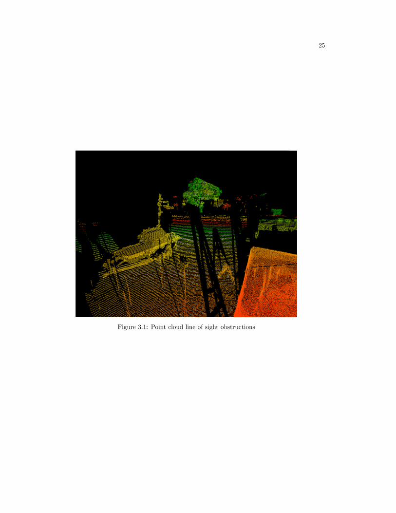
In Figure 3.1 several large locations of scan data appear to be missing. From the sensors per-

spective all pixels are accounted for but when one moves the camera it is apparent that potentially

large areas are unaccounted for. If the point clouds are being converted into other data forms, such

as the heightmap in UAFBot, then these areas present serious concerns.

Depending on the project, missing data from line of sight obstructions may be critical or not.

If robot survival is a primary concern then it is in the best interest to not navigate blindly into un-

mapped terrain. To UAFBot all terrain not explicitly visible on the map was treated as impassible.

In the event that obstructions are presumed temporary, e.g. a person walking through a scene,

then waiting a set amount of time and re-scanning will be sufficient to fill in the occluded area. If

the objects are not expected to move than the robot must change perspectives and combine the

scans.

3.3 Accuracy

All LIDAR have a maximum resolution and accuracy. In general, the more costly the device the

higher these are. The first limiting factor in accuracy is the method used to measure distance.

25

Figure 3.1: Point cloud line of sight obstructions

26

The LMS 291 uses a spinning mirror to reflect an infrared laser beam outwards in a set pattern

and measures the pattern received by the reflected signal. The Kinect projects a known pattern

of infrared dots and uses an IR camera to capture the image. By knowing where a dot ought to

appear and where it is detected in the frame the distance can be calculated.

The precision of scans may be improved by combining multiple scans and removing outliers

although this does little to increase accuracy. It is recommended that the device be calibrated

to conditions that would be typical, including several unusual but not impossible scenarios, for

experimental use. On the LMS 291 there is an indicator marking the plane of the internal sensor

which allows for very precise manual measuring of range. On the Kinect no such line is visible

but images of the dismantled device show the lens to be roughly 1 cm behind the plastic lens

protector. A scan can be taken of static objects with good reflectivity, such as a wall, and the

distance measured precisely via any number of manual methods. If enough distances are analyzed

in this manner a calibration table can be constructed and sensor readings adjusted accordingly.

3.4 Noise

Noise in a LIDAR range scanner is essentially random variance in measurements when there should

be none. A plane perpendicular to the sensor should have all points appear on a flat plane. Often

there will be slight variations in this based on accuracy of the sensor and the material properties of

the object. In general, the further the object the more pronounced the effect.[8] The object being

scanned has a great effect on the scan accuracy as well, a reflective surface at a sharp angle to the

sensor will often not return a signal. Items that are partially transparent to the sensor’s frequencies

may reflect a signal from the surface as well as multiple signals back that have reflected internally,

producing several distances for the same pixel of the scan. How the sensor handles this situation

internally is proprietary, although typically the first signal received is used.

Noise can greatly complicate measuring an area with LIDAR. In particular the closer the scale

of the robot to the noise error the more problematic it becomes. A one cm error when navigating

a car on a highway is likely acceptable but the same error on a robot performing heart surgery is

catastrophic.

There are several known methods for reducing noise; however as it is a property of the underlying

physics, including the uncertainty principle, it cannot ever be completely removed. The simplest

solution is to purchase more advanced scanners. For example the Velodyne HDL-64E has long been

considered the “gold standard” of LIDAR sensors with impressive accuracy, range and sampling

speeds. The price reflects this as it costs around $75,000 USD. When increasing the budget is not

an option other means must be taken.

If noise is a random property simply taking additional scans may be enough to reduce the

variation. Assuming that the noise follows a Gaussian distribution then more samples will reduce

27

the impact of strong outlying points by taking advantage of the central limit theorem. Scans may

also be taken from different locations or perspectives.[9] If the noise itself is random then multiple

scans will improve accuracy; if it is systemic, such as specular reflection, then repeated scans will

not improve accuracy.

Sensor noise is not limited to LIDAR, indeed all sensors suffer from noise in some form or

another. The accelerometer on the Kinect is a fine example of this. During testing it was placed

on a stationary table and still sizable jumps in the acceleration vector were observed. Jitter is an

“abrupt and unwanted variation[s] of one of more signal characteristics...”[10] This trait accurately

describes the effect of the Kinect accelerometer varying far more than one would expect from a

stationary object. The cause is speculatively the overall quality of the accelerometer in the Kinect

as well as it being influenced by the amount of electromagnetic radiation created by other internal

high power consuming components. The methods used to mitigate this sensor jitter are discussed

in detail in the Kinect Results section (see Section 5.4).

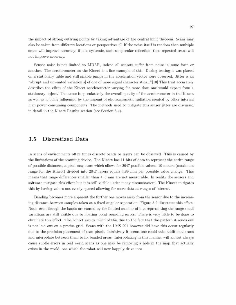
3.5 Discretized Data

In scans of environments often times discrete bands or layers can be observed. This is caused by

the limitations of the scanning device. The Kinect has 11 bits of data to represent the entire range

of possible distances, a pixel may store which allows for 2047 possible values. 10 meters (maximum

range for the Kinect) divided into 2047 layers equals 4.89 mm per possible value change. This

means that range differences smaller than ≈ 5 mm are not measurable. In reality the sensors and

software mitigate this effect but it is still visible under many circumstances. The Kinect mitigates

this by having values not evenly spaced allowing for more data at ranges of interest.

Banding becomes more apparent the further one moves away from the sensor due to the increas-

ing distance between samples taken at a fixed angular separation. Figure 3.2 illustrates this effect.

Note: even though the bands are caused by the limited number of bits representing the range small

variations are still visible due to floating point rounding errors. There is very little to be done to

eliminate this effect. The Kinect avoids much of this due to the fact that the pattern it sends out

is not laid out on a precise grid. Scans with the LMS 291 however did have this occur regularly

due to the precision placement of scan pixels. Intuitively it seems one could take additional scans

and interpolate between them to fix banded areas. Interpolating in this manner will almost always

cause subtle errors in real world scans as one may be removing a hole in the map that actually

exists in the world, one which the robot will now happily drive into.

28

Figure 3.2: Visible banding of ranges in hallway scan

29

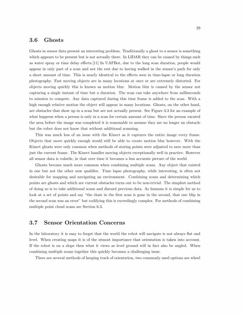
3.6 Ghosts

Ghosts in sensor data present an interesting problem. Traditionally a ghost to a sensor is something

which appears to be present but is not actually there. In LIDAR they can be caused by things such

as water spray or time delay effects.[11] In UAFBot, due to the long scan duration, people would

appear in only part of a scan and not the rest due to having walked in the sensor’s path for only

a short amount of time. This is nearly identical to the effects seen in time-lapse or long duration

photography. Fast moving objects are in many locations at once or are extremely distorted. For

objects moving quickly this is known as motion blur. Motion blur is caused by the sensor not

capturing a single instant of time but a duration. The scan can take anywhere from milliseconds

to minutes to compete. Any data captured during this time frame is added to the scan. With a

high enough relative motion the object will appear in many locations. Ghosts, on the other hand,

are obstacles that show up in a scan but are not actually present. See Figure 3.3 for an example of

what happens when a person is only in a scan for certain amount of time. Since the person vacated

the area before the image was completed it is reasonable to assume they are no longer an obstacle

but the robot does not know that without additional scanning.

This was much less of an issue with the Kinect as it captures the entire image every frame.

Objects that move quickly enough would still be able to create motion blur however. With the

Kinect ghosts were only common when methods of storing points were adjusted to save more than

just the current frame. The Kinect handles moving objects exceptionally well in practice. However

all sensor data is volatile, in that over time it becomes a less accurate picture of the world.

Ghosts become much more common when combining multiple scans. Any object that existed

in one but not the other now qualifies. Time lapse photography, while interesting, is often not

desirable for mapping and navigating an environment. Combining scans and determining which

points are ghosts and which are current obstacles turns out to be non-trivial. The simplest method

of doing so is to take additional scans and discard previous data. As humans it is simple for us to

look at a set of points and say “the chair in the first scan is gone in the second, that one blip in

the second scan was an error” but codifying this is exceedingly complex. For methods of combining

multiple point cloud scans see Section 6.3.

3.7 Sensor Orientation Concerns

In the laboratory it is easy to forget that the world the robot will navigate is not always flat and

level. When creating maps it is of the utmost importance that orientation is taken into account.

If the robot is on a slope then what it views as level ground will in fact also be angled. When

combining multiple scans together this quickly becomes a challenging issue.

There are several methods of keeping track of orientation, two commonly used options are wheel

30

Figure 3.3: Scan showing ghost effect

31

odometry and external sensors. Dead reckoning stores your location and then adjusts it as the robot

moves. We know that the second scan is 12 meters due east of the first scan because the robot

drove 12 meters to the east. This works well in situations where the robot is capable of keeping

accurate track of its motion. In an indoors environment a wheeled robot moving a set distance will

often be highly accurate. The same robot outdoors where it is slipping on ice will have an internal

picture that does not reflect reality.

It is for this reason that most robotic and scanning platforms use external sensors to align their

orientation. GPS is common and can be utilized to high accuracy and even sub-meter precision.[12]

GPS gives you a location not an orientation though. A three-axis accelerometer is helpful for this.

If the robot is not accelerating then the force being applied to the sensor consists solely of gravity.

This allows for the generation of a “down vector,” which as implied by the name, points straight

towards the center of the Earth. The final element of orientation is trickier: that of rotation. In

order to accurately measure rotational acceleration one must add a gyroscope. Gyroscopic sensors

measure angular velocity and are more accurate than dead reckoning techniques for rotation, due

to problems such as slippage mentioned earlier. A combination of measurements from sensors and

internal state dead reckoning offers the highest precision method of tracking a robots movement

through the world. Multiple sensors are commonly combined using a Kalman filter, which creates

a dynamically adjusted weighted average of the inputs.[13]

3.8 Aged Data Culling

In a digital environment data remains correct until something is intentionally changed. The world

is rarely so static. If the robot is placed in a setting where humans and other elements are in

motion then the map needs to be updated over time. This may be nothing more complicated than

a simple point by point replacement, such as new data overwriting the old, or something vastly

more involved. The methodology depends on the precision and timing requirements needed for the

robot.

In the simplest version the image that the robot keeps internally is a fixed size. For the early

version of the Kinect project a matrix of 640 by 480 colors was stored. This proved more than

enough to create attractive scans and to test the specifications of the device. This is advantageous

as a fixed number of points stored is very fast to modify and operate on. The problem is if the

Kinect is rotated or moved then any data not currently in frame is immediately forgotten.

Losing track of data when you cannot see it is obviously not desirable for mapping and UAFBot

used a slightly different technique. Point clouds were saved as individual scans but also possessed

translation and rotation matrices that were computed based on estimations of how far the robot

had moved. By combining them it was thus possible to overlap multiple scans. As discussed earlier

ghosts and artifacts are a chief concern when combining images taken over different time frames.

32

Interestingly as the rate of sampling increases the issues become less pronounced due to a smoothing

effect. Conceptually it is the same as viewing a video at one frame per second versus thirty. In the

former even small movements will be jarring; the latter fast motion may be fluid and traceable.

If we indiscriminately merge two maps taken several minutes apart but from the exact same

orientation and location there still might be differences. If there was a person standing in the first

scan but not the second does the robot still think they are an obstacle? If we decide to discard old

data in preference of more recent and the robot moves then one must be careful. If you drop all

previous data then you may no longer have areas mapped which might be important. How does

one choose which method to keep certain points and not others?

The two main methods experimented with for handling point replacement were dubbed fixed

pool size and time culling. They offered two different ways of accomplishing the same effect of

lessening the impact of old data points and ensuring that the most up to date points were given

due diligence.

Fixed pool size is simply this: the number of points you can store is a fixed number. This

is a multiple of the number of points in a single scan, values between one and ten were tested

on UAFBot with five giving satisfactory results. In concept a circular buffer is used to store the

points. Each scan adds to the total number of points. Once the maximum is reached new samples

begin overwriting existing values starting with the oldest. This continues for as long as scanning is

desired. This methodology has several nice properties. It takes a fixed amount of memory space,

which may be limited on a mobile platform. Data is stored forever as long as scans are not being

taken. If the robot is not mobile then new scans will enhance resolution, which may be helpful if

landmarks are being used to navigate. The downside is that in a fast changing habitat data may

not be culled quick enough. This can be varied by adjusting the multiplier of the scan size to buffer

size but in practice that is set via experimentation early on and is not modified by the robot. The

capacity scale factor is not likely something that could be automated easily to handle changing time

scales of interest. Additionally in the event of continuous scanning the robot will still lose points

that it has not seen in a while, such as those when it first started exploring.

Time culling was the second version of point updating that was tested. Instead of a fixed number

of points a variable size vector containing points is stored. This can be allowed to grow indefinitely

but it would be wise to set a hard limit at which time old data is removed in order to not exhaust

memory. Points are stored with additional meta data. The only data needed for our method was

a life span counter. This was used to determine how much longer the point should be allowed to

persist. An actual time and date of expiration could be used if one is storing very large point clouds

for long periods of time. UAFBot assumed that anything over a certain time frame of importance

had been converted to the internal map representation. As such the life span indicator was a time

stamp which was set with the time of expiration. Every update cycle these values were compared

to the current time. Any points that had a life span of less than or equal to zero were immediately

33

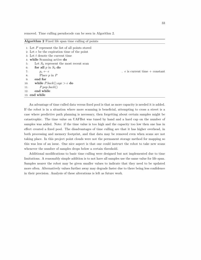
removed. Time culling pseudocode can be seen in Algorithm 2.

Algorithm 2 Fixed life span time culling of points

1: Let P represent the list of all points stored2: Let e be the expiration time of the point3: Let t denote the current time4: while Scanning active do5: Let S0 represent the most recent scan6: for all p in S0 do7: pe ← e . e is current time + constant8: Place p in P9: end for

10: while P.back().age > e do11: P.pop back()12: end while13: end while

An advantage of time culled data versus fixed pool is that as more capacity is needed it is added.

If the robot is in a situation where more scanning is beneficial, attempting to cross a street is a

case where predictive path planning is necessary, then forgetting about certain samples might be

catastrophic. The time value on UAFBot was tuned by hand and a hard cap on the number of

samples was added. Note: if the time value is too high and the capacity too low then one has in

effect created a fixed pool. The disadvantages of time culling are that it has higher overhead, in

both processing and memory footprint, and that data may be removed even when scans are not

taking place. In this project point clouds were not the permanent storage method for mapping so

this was less of an issue. One nice aspect is that one could instruct the robot to take new scans

whenever the number of samples drops below a certain threshold.

Additional modifications to basic time culling were designed but not implemented due to time

limitations. A reasonably simple addition is to not have all samples use the same value for life span.

Samples nearer the robot may be given smaller values to indicate that they need to be updated

more often. Alternatively values further away may degrade faster due to there being less confidence

in their precision. Analysis of these alterations is left as future work.

34

35

Chapter 4

LIDAR

LIDAR, LIght Detection And Ranging, are some of the most commonly used sensor systems in

robotics due to the numerous advantages they possess over other sensors.[14] Stereo-vision as hu-

mans see it has been a research topic for robot designers for decades and while it has progressed

greatly it still has numerous limitations.

One such limitation is the amount of processing power it takes to analyze and manipulate

images in real time. A 1080P resolution webcam can produce a 1920x1080 pixel image at rates

of up to 30Hz. If each pixel is a 32 bit color this is a throughput of 248.8 megabytes per second.

While computers are certainly capable of transferring that much data, one must also be able to do

meaningful work at that rate.

What work must be done is determined by what tasks are to be accomplished. For this paper

the domain will be restricted to robotic navigation. Traditionally this entails creating a map of all

obstacles in the environment, for moving as well as static objects. Next the map is updated and

presented to other systems in a format which can be used for task management and path planning.

In order to create a three-dimensional map that is useful to the robot LIDAR was chosen. Scans

create an image of distances to obstacles from the robot. Using the known angular field of view

for the device the points are then converted using a polar coordinate system to a three-dimensional

Cartesian point cloud. A list of current points is then refreshed each time new scan data arrives

from the LIDAR range sensor.

“LIDAR is an optical remote sensing technology that can measure the distance to, or other

properties of a target by illuminating the target with light, often using pulses from a laser.”[1]

LIDAR sensors use range instead of color to create images. Scans are created by determining

the time of flight between the sent signal and the reflected laser signal pattern. All LIDAR scanners

have different properties, such as range and field of view, but there are many similarities.

Most LIDAR sensors present the data in the form of packets of binary data streaming to the

36

receiver. This is practical due to performance concerns; scans are typically sent many times per

second and need to be captured at the same pace. 30 Hz is one of the most common frequencies of

scan updates.

Often LIDAR scans contain no extra information about the data. For example the Sick LMS

291 does not sense or indicate its orientation in the world. In robotics knowing whether you are

on an incline or even upside down greatly affects the map being created. LIDAR leaves this to

additional sensors. However the Kinect 360 includes a three-axis accelerometer.

LIDAR are frequently used in measuring atmospheric conditions[15] as well as for surveying and

mapping. The high precision and range of laser range finders lends them to conditions where taking

direct physical measurements is either impractical or impossible.

4.1 Sick LMS 291

The Sick LMS 291 has established itself as one of the most commonly LIDAR used in the robotics

world.[16] The relatively small size, high accuracy and range make it a valuable sensor for moving

platforms. The strongest downside is the high cost, with prices ranging between $3000-$7000 USD

over the years, which precludes its use on less well funded projects.

Other concerns noted are the moderately high weight, an issue on compact or platforms with

strong weight restrictions such as UAVs. The weight comes from the durable design which is robust

to real world wear and tear, especially when compared to the fragile nature of most precision

measuring instruments. It also requires a nontrivial amount of power to operate, up to 30 Watts

for continuous usage. For more detailed specifications see Table 4.1.

4.2 Kinect

The Kinect is a relative newcomer in the sensor world and has rapidly grown in popularity among

robotics researchers and designers. The version of the Kinect tested in this paper (Xbox 360 Kinect)

has the following hardware sensors accessible for use: optical camera, IR range camera, (4) audio

sensors and a three-axis accelerometer. All of this hardware in a relatively small package seems

ready made for the researcher with a budget. Coming in at just $150 USD one could purchase over

twenty Kinects for the price of one Sick LMS 291.[17]

At product launch there was no way for a developer to access the hardware as drivers were not

provided by Microsoft. An engaged online community, spurred by a $3000 USD bounty, rapidly

reverse engineered the Kinect’s communication protocol, releasing working software in November

2010.[18] In March 2011 Microsoft released their own set of drivers for the device called the Kinect

SDK.[19]

37

4.3 Comparison

The LMS 291 and the Kinect have many similarities. They present scan data at similar resolutions

and update frequencies. Other than physical characteristics the chief difference is the scan range.

The Kinect has a maximum range of 10 meters and several papers report that for highest accuracy

under 5 meters is desirable.[20] The LMS 291 on the other hand has an effective range of 80 meters

and in my experience is usably accurate to that range. The Kinect creates an image of 640 by 480

range values every update whereas the LMS 291 only creates a single scan-line. The resolution of

the LMS 291 can be varied by the user, the maximum number of 401 values per 100 degree field of

view scan was used on UAFBot.

In order to create a two-dimensional image of samples using the LMS 291, or a similar device,

the LIDAR range sensor must be moved in a known manner. In the UAFBot project the LMS 291

was mounted to a platform rotated by a stepper motor controlled via the control software. In

this manner the scanning software always knew where the LIDAR pointed and could orient the

points properly. The advantage is that the field of view could be adjusted to optimize for the scans

required at the time. The disadvantage is that moving hardware is slow. Stepping in sub-degree

angles for an entire 360 degree panorama took over three minutes using UAFBot. This produced

a very high detail environment map of static objects but was useless when attempting to capture

moving objects.

The Kinect on the other hand utilizes an infrared projected pattern beamed out of the device.

The IR camera then reads an image and powerful onboard hardware analyzes the pattern to compute

the distances. One can confuse a Kinect using a hand-held IR laser pointer with a frequency near

830 nm. Anecdotal experiments trying to distract input to the LMS 291 were met with failure, there

is a very small window of both frequency and time that can corrupt scans intentionally. Table 4.1

displays specifications for both the Kinect and LMS 291 in detail.

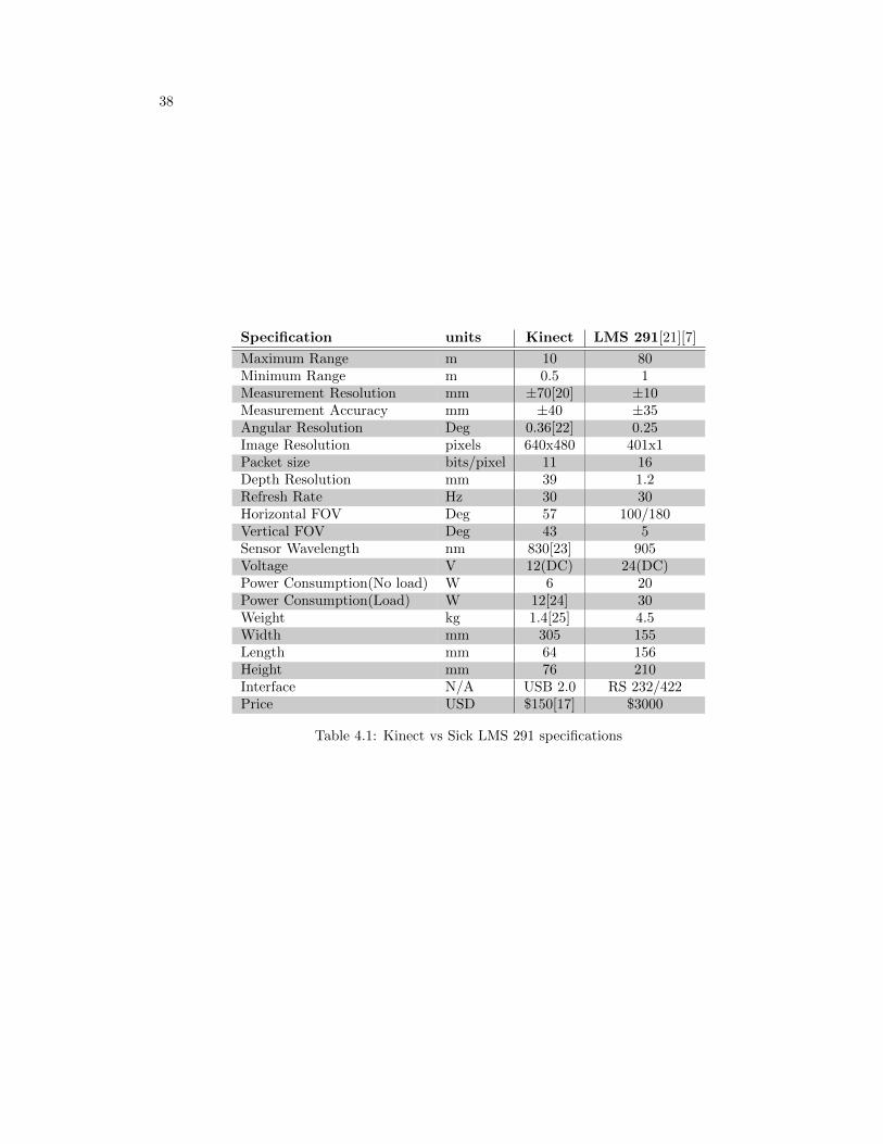
38

Specification units Kinect LMS 291[21][7]

Maximum Range m 10 80Minimum Range m 0.5 1Measurement Resolution mm ±70[20] ±10Measurement Accuracy mm ±40 ±35Angular Resolution Deg 0.36[22] 0.25Image Resolution pixels 640x480 401x1Packet size bits/pixel 11 16Depth Resolution mm 39 1.2Refresh Rate Hz 30 30Horizontal FOV Deg 57 100/180Vertical FOV Deg 43 5Sensor Wavelength nm 830[23] 905Voltage V 12(DC) 24(DC)Power Consumption(No load) W 6 20Power Consumption(Load) W 12[24] 30Weight kg 1.4[25] 4.5Width mm 305 155Length mm 64 156Height mm 76 210Interface N/A USB 2.0 RS 232/422Price USD $150[17] $3000

Table 4.1: Kinect vs Sick LMS 291 specifications

39

Chapter 5

Kinect Project

With the release of the MicrosoftTMKinect, consumer affordable range-finding devices became avail-

able for the first time. It was decided that in order to evaluate the Kinect and its potential a project

was necessary. The goal for Kinect Project was to replicate the work done prior on UAFBot, without

the mobile robotic platform.

5.1 Requirements

By far the most complicated aspect of this project was the real-time communication with asyn-

chronous hardware. Several considerations were taken into account in order to ensure operation

met the project requirements.

As discussed in the UAFBot section, functional requirements are properties of what the system

should be capable of. There are many similarities between the UAFVision system and the Kinect

Project. Otherwise comparison between the two would be difficult.

• Kinect software will be readable and extensible for future experiments.

• Software will not introduce noticeable time delay into scanning.

• Project will be designed such that it is possible to compare LMS 291 and Kinect results.

• Software will compile on a standard Linux platform.

The two main categories of non-functional requirements that were most relevant to this project

were performance and maintainability. Performance was concerned with meeting the real-time

demands of both the hardware and rendering as well as ensuring the user interface responded in a

timely manner. Maintainability forced the program to be would written and documented in such a

40

way that others will be able to use or expand upon it at a later date without requiring contacting

the original developer (myself).

Performance Requirements

• PE-1: The software shall maintain exclusive control over the Kinect when operating.

• PE-2: The software shall read data from the Kinect at the hardware’s optimal rate, currently

known to be 30 Hz.

• PE-3: The software shall render updates to the rendering screen no slower than 15 Hz.

• PE-4: User input to the software shall be accepted and utilized no later than the next frame.

Maintainability Requirements

• MA-1: The code shall be written using known best standards and practices.

• MA-2: The project shall be documented in such a way that future maintenance is straight

forward to someone unfamiliar to the code.

• MA-3: Code comments will document the “why,” not just what is.

• MA-4: Source code shall be stored in a version control repository.

5.2 Design

The Kinect project was simpler than UAFBot for one major reason: it did not require the con-

struction of a robot. Based on the schedule from UAFBot this was immediately a 50% reduction

in time involvement. Additionally many lessons learned would be applicable. Code that was too

tightly coupled to be used directly was analyzed to duplicate core functionality. This allowed for a

much more compact development cycle. Indeed the Kinect project was very nearly developed using

the Waterfall method.

The final goal of the Kinect project was to recreate the scanning, point cloud conversion, and

heightmap generating functionality from UAFBot using a different scanning device. This was

simplified by the fact that point clouds are nearly a universal format, once the unit values and

field-of-views are known translations between systems are simple.

41

Project Requirements

Prior experience with range-finding sensors simplified designing this project. This feature was con-

cerned with coming up with the specific requirements and which experiments to attempt. Similarity

with the UAFBot project was required so that results could be readily compared.


Pre-reqs: None

LibFreeNect

At the time only LibFreeNect was available as a driver package for the Kinect. As one might expect

of a small open source project documentation was scarce. Considerable time was estimated for

this feature as often even compiling the source of an open source project can be problematic. The

library choice constrained the project to Linux as Windows has specific requirements for drivers to

be signed and approved, which LibFreeNect most certainly did not meet.


Pre-reqs: Project Requirements

Talk to Kinect

Once the driver software was installed and compiled then communicating with the Kinect became

possible. This required codifying the Kinect protocol into the framework. A framework for handling

messages back and forth was necessary. It was also required to be thread safe due to the methods

of connecting a USB driver to a device.


Pre-reqs: LibFreeNect

Read Scans

Kinect scans were read in from a USB device which communicated in a different manner from the

LMS 291. Data was received asynchronously as opposed to per request. This required a different

system for handling data input. Kinect scan data was also not measured in units of distance but

in parallax disparity. Thus it must be interpreted before it could be converted to a point cloud.


Pre-reqs: Talk to Kinect

OpenGL GUI

The GUI program was responsible for rendering the output of a point cloud as well as any user

input for manipulating the view. The program handled reading scans from the Kinect, converting

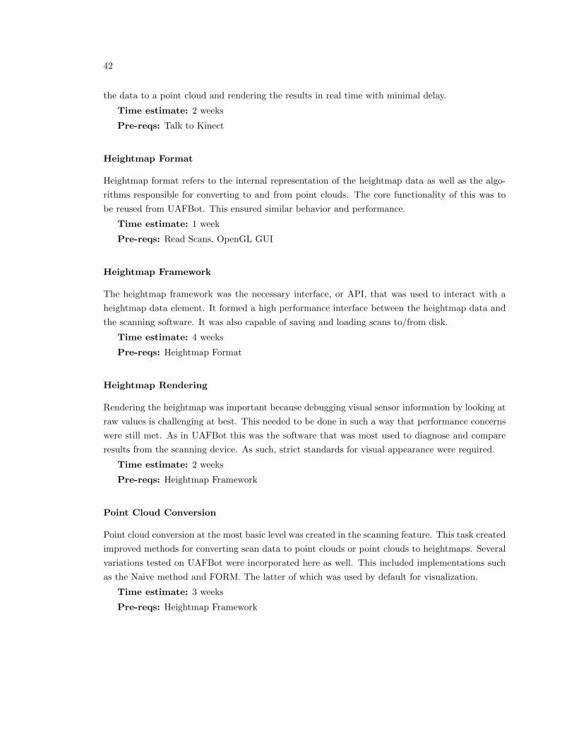
42

the data to a point cloud and rendering the results in real time with minimal delay.


Pre-reqs: Talk to Kinect

Heightmap Format

Heightmap format refers to the internal representation of the heightmap data as well as the algo-

rithms responsible for converting to and from point clouds. The core functionality of this was to

be reused from UAFBot. This ensured similar behavior and performance.


Pre-reqs: Read Scans, OpenGL GUI

Heightmap Framework

The heightmap framework was the necessary interface, or API, that was used to interact with a

heightmap data element. It formed a high performance interface between the heightmap data and

the scanning software. It was also capable of saving and loading scans to/from disk.


Pre-reqs: Heightmap Format

Heightmap Rendering

Rendering the heightmap was important because debugging visual sensor information by looking at

raw values is challenging at best. This needed to be done in such a way that performance concerns

were still met. As in UAFBot this was the software that was most used to diagnose and compare

results from the scanning device. As such, strict standards for visual appearance were required.


Pre-reqs: Heightmap Framework

Point Cloud Conversion

Point cloud conversion at the most basic level was created in the scanning feature. This task created

improved methods for converting scan data to point clouds or point clouds to heightmaps. Several

variations tested on UAFBot were incorporated here as well. This included implementations such

as the Naive method and FORM. The latter of which was used by default for visualization.


Pre-reqs: Heightmap Framework

43

Read Accelerometer

An interesting bonus element of the Kinect was the three-axis accelerometer. This allowed reading

in the direction of gravity, assuming no additional acceleration forces. This task created code which

interpreted the raw sensor data and formed a directional vector in real time.


Pre-reqs: Heightmap Rendering, Point Cloud Conversion

Point Cloud Alignment

Aligning the point cloud with the accelerometer data required creating a rotation matrix based on

the current down vector and multiplying it against all points in the cloud. This was done every

frame so that altering the Kinect’s orientation was captured correctly. Only rotation about the

front/back and left/right axis could be computed with this sensor. A gyroscope or similar sensor

would be necessary to track rotation about the vertical axis and was not implemented.


Pre-reqs: Read Accelerometer

5.3 Schedule

Stage 0

Stage 0 involved simply communicating with the device. As with all hardware and software com-

munications this is often more difficult than simply plugging in the device and sending commands.

This stage was mostly set aside as a learning time to understand the preliminary limitations of the

hardware and software library used to operate it. This stage was completed upon the successful

compilation and execution of demonstration software provided by the software library developers.

The software used to interface with the Kinect was OpenKinect as Microsoft had not released a

development environment at the time. This library is open source under the GPL2 License.[26] It

is cross platform and runs on Windows, Linux and Mac. Due to known limitations with Windows

and USB drivers the project was written using a Linux platform.

Stage 1

Stage 1 expanded upon Stage 0 and added additional functionality for testing and debugging in a

visual environment. Raw sensor data is much more difficult to analyze and verify than a picture.

OpenGL was chosen to render the data due to its familiarity and availability in the chosen develop-

ment environment. Completion of Stage 1 involved connecting to the Kinect, reading sensor data

in real time, and rendering that data to the screen above minimal refresh rates.

44

Stage 2

Stage 2 added the conversion from raw sensor points to a functional heightmap. The methods used

are explained in detail in other sections. Heightmaps were a key test as there are many well known

techniques for navigating robots within them. If a complicated real-world environment could be

converted to a heightmap then traversing them would be much less computationally expensive; a

strong positive when dealing with the strict real time complexities of robotic navigation.

Stage 3

Stage 3 was intended to tie the project together by adding usability and cosmetic upgrades to

enhance the user experience. One way this was implemented was by using the built in accelerometer

to correct for alignment issues of the sensor. When creating a two-dimensional map it is very

important that the plane of the map be parallel to the true plane of the ground, defined here as

perpendicular to the gravity vector of the Earth. As long as all sensor data could be correctly

aligned with gravity then map accuracy is greatly enhanced. If one scan is aligned and another is

tilted at an angle without correction it would appear that the ground is now sloping at an angle

either towards or away from the robot – neither of which is correct.

Additionally the heightmap visualization were made more attractive as well as more useful by

having the ability to navigate the scene via user input. All of these additions made the project

more useful as a demonstration and testing environment to show off the Kinect’s data gathering

ability.

5.4 Kinect Project Results

At the beginning of the project it was obvious that drivers for the Kinect were in an early stage

of development. As is often the case documentation was limited to a small number of example

programs and mailing lists discussing various bugs. Often innocuous seeming changes to example

programs would render cryptic compile error messages or code simply refusing to run. With the

assistance of several helpful members of the LibFreeNect message board, connecting to the Kinect

was accomplished.

One of the more interesting aspects of the software related to the fact that unlike the LMS 291

the Kinect did not send range values in standard units. On the LMS 291 units are in integer

centimeters by default. On the Kinect they are parallax disparity values which were then converted

by a formula to units of distance. These values were found experimentally by a volunteer as no

official documentation was available.[27] See Algorithm 3 for the exact equation used.

One immediately obvious aspect of the Kinect was the relatively narrow field of view. 57◦ in the

horizontal plane and 43◦ in the vertical may not sound narrow but it is the equivalent of a 50 mm

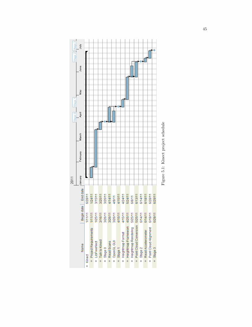
45

Fig

ure

5.1

:K

inec

tp

roje

ctsc

hed

ule

46

Algorithm 3 Converting raw Kinect data to meters (i, j, k)→ (x, y, z)

1: m← −0.037 . m was determined experimentally2: fov ← 0.0021 . fov is the field of view per pixel3: i and j are the coordinates in the image4: k is the raw value of the image at (i, j)5: x← (i− (w/2))(z +m)fov(w/h)6: y ← (j − (h/2))(z +m)fov7: z ← 0.1236 tan(k/2842.5 + 1.1863)

camera lens in terms of zoom. The LMS 291 field of view is approximately a 18 mm lens.[28] This

narrow field of view complicated scanning a wide area as it quickly became necessary to combine

multiple scans to cover even a small room.

The range was also of concern with the Kinect. Many papers have studied the accuracy of the

Kinect and found it to be quite accurate in the range of approximately one to ten meters. Outside

that range the data rapidly becomes inaccurate or simply unobtainable. This in sharp contract to

the LMS 291’s range of 80 meters.

As noted the accelerometer on the Kinect was incorporated in order to provide orientation to

the points being scanned. This sensor was subject to massive amounts of jitter regardless of the

stability of the table it was resting on. When the point cloud was rotated according to the current

down vector, as updated each frame, tilting of up to 30◦ left or right were common, the image moved

so much as to be unrecognizable. The solution was to add a dampening effect on the accelerometer

data. Instead of normalizing the scan against the raw sensor value a time weighted average was

implemented. The accelerometer updated at 30 Hz and the number of values used in the weighted

average was varied between 1 and 30 to experiment with the effects. In the end 10 was selected due

to being a fair compromise. With low numbers the effect of averaging was not visible and with high

numbers a noticeable lag between tilting the sensor and the scan correctly rotating occurred. With

1/3 of a second to replace the true value points no longer jumped around but moving the Kinect

did not cause a great delay in the data properly orienting itself to match the sensor. Algorithm 4

shows the weighting function used, p was set to 10 in the Kinect project.

Algorithm 4 Time Weighting Function

Let p be the proportional value, p ≥ 1vstable ← (0,−1, 0)while updating accelerometer do

v← sensorvstable ←

(1p

)v +

(1− 1

p

)vstable

end while

Experimentation with the Kinect showed it also had more difficulties with sunlight than the

47

LMS 291. The LMS 291 has the advantage of transmitting all laser signal power into each scan

whereas the Kinect spreads its power across the 640 by 480 pixels. The sensor frequencies for the

Kinect and LMS 291 are 830 nm and 905 nm respectfully. Interestingly there is quite a difference

in the power the sun outputs at those frequencies despite how close they are. At 830 nm the

sun produces 1.0563[Wm−2nm−1] and at 905 nm only 0.918[Wm−2nm−1], a 13% decrease in raw

energy.[29] That is not enough to account for the inaccurate scans of the Kinect but it was worth

noting. Even indoors, sunlight entering a window was sometimes enough for the Kinect to lose

partial or all sensor data. The LMS 291 had no noticeable difference indoors versus direct sunlight.

For an in depth comparison of the specifications for the LMS 291 and Kinect see Table 4.1.

5.5 Future Work

Future work to improve the usability of the Kinect might incorporate additional onboard sensors.

The visual camera was not utilized in the Kinect project and could add more data to a point cloud

by setting a true color for each point. Other research can be found using this technique and it

appears promising. It seems far more useful to humans attempting to recognize objects than to a

robot navigating however.

Another feature left to later testing was that of taking multiple scans from different locations

and/or angles and combining them. The most difficult aspect of combining point clouds is knowing

precisely the location of the scans relative to each other. Based on the results of the Kinects

accuracy there is no technical reason this could not be done, provided the scans are within the

maximum accuracy range of < 10 m.

Since the beginning of this project several new libraries were released, notably OpenKinect

and the official Kinect SDK. Recreating the Kinect project using these libraries would be a useful

learning experience. The Kinect SDK has numerous additional features that could be utilized for

more advanced testing as well.

And finally the new version of the Kinect is under development. It is slated for public release

sometime in 2014.[30] Early press releases show a marked increase in performance and capabilities.

If the device fixes some of the flaws in the current Kinect it stands to become an exceptional sensor

for the price range.

48

49

Chapter 6

Data Formats

Choosing the proper data format for mapping and navigating is critical for robotic platforms. A

poorly chosen format makes path planning and goal completion complicated or inefficient. The map

and data structure must be selected based on the criteria for the specific project. A robot designed

to operate in a factory painting cars has different needs from a rover exploring new worlds.

6.1 Point Clouds

Point clouds represent data points in a coordinate system, most commonly utilizing three-dimensional

Cartesian space.[31] Point clouds are used in many fields such as manufacturing and surveying. As

previously discussed LIDAR devices are well suited to creating point cloud based data. This is

due to the simple method necessary to convert range images to point clouds. The image can be

thought of as in spherical coordinates. The radial angle, φ, is the current location in the horizontal

axis; θ, is the azimuth, which is in vertical axis; and the value is the distance r. One can compute

the φ and θ values based on the pixel coordinates in the image and the field-of-view angle in both

dimensions. Algorithm 5 converts image coordinates to Cartesian coordinates. fov stands for the

field-of-view in degrees, w and h for the image width and height in pixels respectfully. ∆φ and ∆θ

are the degrees between each pixel in the scan, for example 1/4◦ is default for the LMS 291. It is

important to note that this only applies to the LMS 291, the Kinect uses a rectilinear coordinate

system. i and j should be centered (0, 0) for the image, although this adjustment is not included

in Algorithm 5 to simplify the example.

While combining multiple scans in points clouds is simple, the aspect of registering the scans

may be complicated. Many methods are available. The simplest method is to precisely measure

the locations of the scans so that corrections will be minor and merely fine adjustments.[32] The

various forms of image registration are beyond the scope of this paper however.

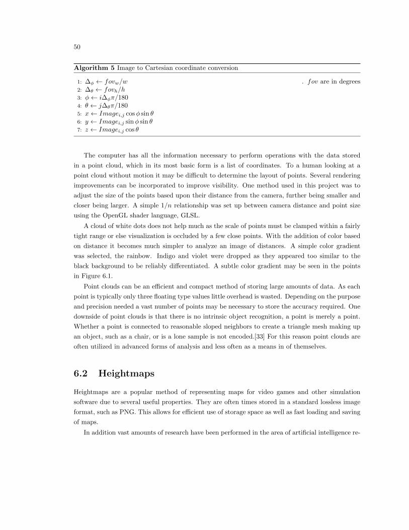
50

Algorithm 5 Image to Cartesian coordinate conversion

1: ∆φ ← fovw/w . fov are in degrees2: ∆θ ← fovh/h3: φ← i∆φπ/1804: θ ← j∆θπ/1805: x← Imagei,j cosφ sin θ6: y ← Imagei,j sinφ sin θ7: z ← Imagei,j cos θ

The computer has all the information necessary to perform operations with the data stored

in a point cloud, which in its most basic form is a list of coordinates. To a human looking at a

point cloud without motion it may be difficult to determine the layout of points. Several rendering

improvements can be incorporated to improve visibility. One method used in this project was to

adjust the size of the points based upon their distance from the camera, further being smaller and

closer being larger. A simple 1/n relationship was set up between camera distance and point size

using the OpenGL shader language, GLSL.

A cloud of white dots does not help much as the scale of points must be clamped within a fairly

tight range or else visualization is occluded by a few close points. With the addition of color based

on distance it becomes much simpler to analyze an image of distances. A simple color gradient

was selected, the rainbow. Indigo and violet were dropped as they appeared too similar to the

black background to be reliably differentiated. A subtle color gradient may be seen in the points

in Figure 6.1.

Point clouds can be an efficient and compact method of storing large amounts of data. As each

point is typically only three floating type values little overhead is wasted. Depending on the purpose

and precision needed a vast number of points may be necessary to store the accuracy required. One

downside of point clouds is that there is no intrinsic object recognition, a point is merely a point.

Whether a point is connected to reasonable sloped neighbors to create a triangle mesh making up

an object, such as a chair, or is a lone sample is not encoded.[33] For this reason point clouds are

often utilized in advanced forms of analysis and less often as a means in of themselves.

6.2 Heightmaps

Heightmaps are a popular method of representing maps for video games and other simulation

software due to several useful properties. They are often times stored in a standard lossless image

format, such as PNG. This allows for efficient use of storage space as well as fast loading and saving

of maps.

In addition vast amounts of research have been performed in the area of artificial intelligence re-

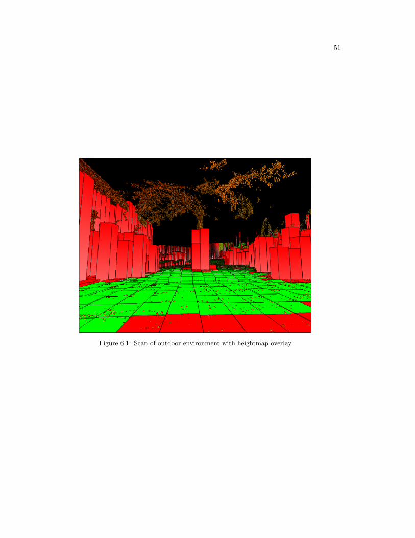
51

Figure 6.1: Scan of outdoor environment with heightmap overlay

52

garding heightmaps. One of the best known algorithms for path-finding in a grid-based environment

is A* (pronounced A-star).[34]

Heightmaps are simple two-dimensional matrices storing a value which is commonly a height,

hence the name. Sizes may be bounded or allowed to grow as necessary depending on implementa-

tion. The most complicated aspect of preparing a heightmap for an area is deciding the scale of the

grid. The two axes may be independently scaled, although most implementations utilize a square

grid as it allows for additional computing shortcuts. The scale must be chosen with care. If the

cells are too large then we are creating the equivalent of a low resolution image. Single cells may

represent vast ranges in true data but are unable to properly encode it. The smaller the scale of

cells the more accurate the heightmap but the larger the memory footprint becomes. The project

must determine the scale required. For example, UAFBot is approximately one meter square in

footprint. One might assume that selecting a scale of one meter per cell would be correct and while

it is a fine starting place it is less than ideal. If we decide the robot needs a cell plus adjacent

cells available to drive through then we require three cells to traverse. Very few doorways are three

meters wide so our robot would be unable to pass, even though in reality it would easily fit. A scale

of 0.25 meters by 0.25 meters was used in UAFBot for general purposes. This created a detailed

enough map but allowed for somewhat tight passage of the robot.

Heightmaps present a compact means of storing data. As mentioned a standard resolution

image may contain information for a map many kilometers on a side depending on how large the

scale value is. Visually they are easy to understand as well, many times it simply appears that all

objects have been surrounded by axis-aligned rectangular bounding boxes. Path-finding is straight

forward as most path-finding algorithms are graph searching in nature and heightmaps are graphs

where each cell is a node connected to its adjacent neighboring cells.

One of the most severe limitations of traditional heightmaps is that each cell may represent only

a single value. There is no way to map overhanging objects without losing potentially important

data. Either the floor is set as the height or the top of the obstacle is. Figure 6.2 illustrates an

obstacle that correctly has multiple values for height depending on application. Caves or buildings

with multiple floors suffer from this limitation as well.

6.3 Converting Point Clouds to Heightmaps

Mathematically there is nothing difficult or computationally expensive about converting a three-

dimensional point cloud to a two-dimensional heightmap but some subtle results arise from various

methods. Conceptually the goal is to create a map in which the floor is flat and the obstacles

are indicated by being taller than the ground. If the software must function both indoors and out

several cases occur which produce interesting incorrect results when using basic algorithms.

One complication that must be considered is how to handle heightmap cells which have no

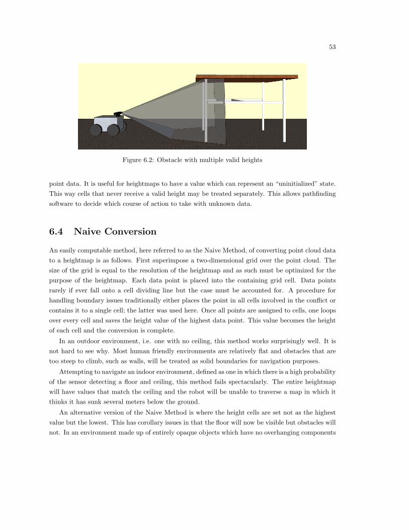
53

Figure 6.2: Obstacle with multiple valid heights

point data. It is useful for heightmaps to have a value which can represent an “uninitialized” state.

This way cells that never receive a valid height may be treated separately. This allows pathfinding

software to decide which course of action to take with unknown data.

6.4 Naive Conversion

An easily computable method, here referred to as the Naive Method, of converting point cloud data

to a heightmap is as follows. First superimpose a two-dimensional grid over the point cloud. The

size of the grid is equal to the resolution of the heightmap and as such must be optimized for the

purpose of the heightmap. Each data point is placed into the containing grid cell. Data points

rarely if ever fall onto a cell dividing line but the case must be accounted for. A procedure for

handling boundary issues traditionally either places the point in all cells involved in the conflict or

contains it to a single cell; the latter was used here. Once all points are assigned to cells, one loops

over every cell and saves the height value of the highest data point. This value becomes the height

of each cell and the conversion is complete.

In an outdoor environment, i.e. one with no ceiling, this method works surprisingly well. It is

not hard to see why. Most human friendly environments are relatively flat and obstacles that are

too steep to climb, such as walls, will be treated as solid boundaries for navigation purposes.

Attempting to navigate an indoor environment, defined as one in which there is a high probability

of the sensor detecting a floor and ceiling, this method fails spectacularly. The entire heightmap

will have values that match the ceiling and the robot will be unable to traverse a map in which it

thinks it has sunk several meters below the ground.

An alternative version of the Naive Method is where the height cells are set not as the highest

value but the lowest. This has corollary issues in that the floor will now be visible but obstacles will

not. In an environment made up of entirely opaque objects which have no overhanging components

54

the ground is now correctly detected. However, in cases where obstacles can be partially seen

through but not safely traversed, such as a fence, these obstacles are ignored and are not present

in the heightmap data. In fact nearly all obstacles will be ignored, which poses disastrous results

for the robot attempting to navigate. The algorithm describing the Naive method can be found in

Algorithm 6.

Algorithm 6 Naive Point Cloud conversion

1: Let P represent all samples in the point cloud2: Create 2 dimensional matrices to store values called M3: for all samples s in P do4: i = floor(sx/gridsizex)5: j = floor(sz/gridsizez)6: Mi,j = max(Mi,j , sy)7: end for

6.5 FORM Conversion

To overcome the limitations of the Naive Method, a new method was devised for the purpose of this

project. FORM (Floor Obstacle Roof Method) operates as such: All point cloud data samples are

constrained to heightmap cells, the same as in the Naive method. The highest and lowest points

in that cell are set as the floor and ceiling of the cell. Next the highest point that the robot might

contact is saved as the obstacle height of the cell. Any point that occurs between the floor and

floor plus robot height would cause a collision and is thus an obstacle. Any points above floor

plus robot height would not contact the robot and can be ignored. This is performed for each cell

until the heightmap is fully generated. The floor and ceiling values can either be saved to create

additional heightmaps or be discarded if memory space is more important. In the default version

FORM discards this data.

The idea behind FORM is that many obstacles the Naive Method detects are in fact safely

passable by the robot. The robot used for testing measured 0.8 meters in height therefore any

surface with a reasonably level slope that had over 1 meter clearance could be driven underneath

with no concern. This also eliminated the problem of the robot being unable to navigate through

doorways. Intuitively this makes sense as one is not concerned with colliding with a three meter

high ceiling during their day to day activities; only when we might strike our head on a low hanging

beam do we have to possibly change routes.

FORM overcomes the main limitation of the Naive method of conversion in that it creates

practical maps in environments that have both floors and ceilings. By allowing the robot to drive

underneath obstacles that may be marked as safe, additional knowledge is effectively coded into the

55

heightmap compared to other methods. FORM does not allow a heightmap to be used in complex

three-dimensional layers however; heightmaps are more efficient on relatively level surfaces. While

FORM does not solve all the limitations in navigation using a heightmap it represents a significant

step forward in the effectiveness of point cloud generated heightmaps. The FORM pseudocode can

be found in Algorithm 7. See Figure 6.1 for an example of FORM deciding a tree trunk is not

passable but the robot may still travel underneath the high branches.

Algorithm 7 FORM Point Cloud conversion

1: Let P represent all samples in the point cloud2: Let h represent the max height of the robot3: Create 2 dimensional matrices H to store height values4: and F to store floor values5: for all samples s in P do6: i = floor(sx/gridsizex)7: j = floor(sz/gridsizez)8: Fi,j = min(Fi,j , sy)9: end for

10: for all samples s in P do11: i = floor(sx/gridsizex)12: j = floor(sz/gridsizez)13: if sy < Fi,j + h then14: Hi,j = max(Hi,j , sy)15: end if16: end for

56

57

Chapter 7

Concluding Remarks

This project was created in multiple phases, the first was to develop a robotic platform and test

the Sick LMS 291. The development of UAFBot met the requirements for the physical chassis

and platform and the software developed in UAFVision incorporated the LIDAR scans into the

digital realm. One of the most important lessons learned from UAFBot was the importance of

putting a large amount of effort into designing hardware. Software has a cost to modify after it is

created, measured in units of person-time, but hardware requires time and parts and shop time and

more. It is therefore important to think of what might be done with the robot as well as how it

will most likely be used. Knowing in advance that all components will likely either be replaced or

broken allowed us to design a robot that had simplified and streamlined maintenance. UAFVision

taught several lessons as well. First: never underestimate the effort required to communicate with

hardware in a timely and exception safe manner. It is always important to verify that data sent to

and, especially, being received from a sensor is valid and usable. Overall orienting the LIDAR on

its side to create a vertical scan-line allowed for a more controllable field of view when scanning.

With high range, accuracy and refresh rate the Sick LMS 291 has certainly earned its position as

one of the most popular range-detecting sensors in the world today.

Point clouds and heightmaps are data structures which excel in specific areas. In this paper

it has been shown how to create point clouds from range-detecting sensors. Point clouds may be

used as stand alone data structures for either analysis or navigation. With the development of a

new algorithm, FORM, point clouds can be converted into heightmaps for use as navigation tools.

Heightmaps excel as maps for the reason that they can be searched by path-finding algorithms

efficiently.

Comparing the LMS 291 to the Kinect was an interesting experience. The two devices are similar

in overall concept yet quite different in practicality. The LMS 291 wins in nearly all categories that

are of utmost importance in a range sensor: it has much more range, is a little more accurate and

58

has a larger field of view. The Kinect produces images instead of single lines of data at the exact

same rate and costs 1/20 as much which makes for a very practical sensor.

Software engineering principles are useful to all projects, especially those that typically would

not follow such formal methods. Trying to apply solid management practices to a student volunteer

project is no small feat. Many project members became converts when planning or scheduling tasks

in advance saved a considerable amount of time and effort. In my experience people overlook tools

until they see a tangible immediate benefit for them. Eliciting features and requirements at the

beginning of the project allowed people to work later without constantly having to question stake

holders about specific cases.

There will always be advances in the fields of robotics and sensors and I personally look forward

to testing what the next generation of hardware is capable of.

59

References

[1] A. P. Cracknell, Introduction to Remote Sensing. CRC Press, second edition ed., 2007.

[2] C. Murphy, D. Lindquist, A. M. Rynning, T. Cecil, S. Leavitt, and M. L. Chang, “Low-

Cost Stereo Vision on an FPGA,” in Field-Programmable Custom Computing Machines, 2007.

FCCM 2007. 15th Annual IEEE Symposium on, pp. 333–334, IEEE, 2007.

[3] B. W. Boehm, “A Spiral Model of Software Development and Enhancement,” Computer,

vol. 21, pp. 61 –72, may 1988.

[4] I. Sommerville, Software Engineering. Harlow, England New York: Addison-Wesley, 2007.

[5] K. E. Wiegers, Software Requirements 2. Microsoft Press, 2nd ed. ed., 2003.

[6] S. McConnell, Software Estimation: Demystifying the Black Art: Demystifying the Black Art.

O’Reilly Media, Inc., 2009.

[7] SICK, “Developer’s Guide.” http://www.sickcn.com/media/89813/developers_guide_

lms1xx_5xx_v3.6.pdf.

[8] M. Pauly, N. J. Mitra, and L. Guibas, “Uncertainty and Variability in Point Cloud Surface

Data,” in Symposium on Point-Based Graphics, vol. 9, 2004.

[9] J. C. Carr, R. K. Beatson, J. B. Cherrie, T. J. Mitchell, W. R. Fright, B. C. McCallum, and

T. R. Evans, “Reconstruction and Representation of 3D Objects with Radial Basis Functions,”

in Proceedings of the 28th annual conference on Computer Graphics and Interactive Techniques,

pp. 67–76, ACM, 2001.

[10] F. Standard, “1037C. Telecommunications: Glossary of Telecommunication Terms,” Institute

for Telecommunications Sciences, vol. 7, 1996.

[11] R. Rasshofer and K. Gresser, “Automotive Radar and Lidar Systems for Next Generation

Driver Assistance Functions,” Advances in Radio Science, vol. 3, no. 10, pp. 205–209, 2005.

http://www.sickcn.com/media/89813/developers_guide_lms1xx_5xx_v3.6.pdf

http://www.sickcn.com/media/89813/developers_guide_lms1xx_5xx_v3.6.pdf

60

[12] S. M. Lichten, “Estimation and Filtering for High-Precision GPS Positioning Applications,”

Manuscripta Geodaetica, vol. 15, pp. 159–176, 1990.

[13] G. Welch and G. Bishop, “An Introduction to the Kalman Filter,” 1995.

[14] F. Amzajerdian, D. F. Pierrottet, L. B. Petway, G. D. Hines, and V. E. Roback, “Lidar Systems

for Precision Navigation and Safe Landing on Planetary Bodies,” Imaging, vol. 2, 2011.

[15] F. G. Fernald, “Analysis of Atmospheric Lidar Observations- Some Comments,” Applied Op-

tics, vol. 23, no. 5, pp. 652–653, 1984.

[16] M. Montemerlo, J. Becker, S. Bhat, H. Dahlkamp, D. Dolgov, S. Ettinger, D. Haehnel,

T. Hilden, G. Hoffmann, B. Huhnke, et al., “Junior: The stanford entry in the urban chal-

lenge,” Journal of Field Robotics, vol. 25, no. 9, pp. 569–597, 2008.

[17] N. Rafibakhsh, J. Gong, M. K. Siddiqui, C. Gordon, and H. F. Lee, “Analysis of XBOX

Kinect Sensor Data for Use on Construction Sites: Depth Accuracy and Sensor Interference

Assessment,” in Constitution Research Congress, pp. 848–857, 2012.

[18] Adafruit, “We Have a Winner: Open Kinect Drivers Released.” http://www.adafruit.com/

blog/2010/11/10/we-have-a-winner-open-kinect-drivers-released-winner-will-

use-3k-for-more-hacking-plus-an-additional-2k-goes-to-the-eff/, November 2010.

[19] R. Knies, “Academics, Enthusiasts to Get Kinect SDK.” http://research.microsoft.com/

en-us/news/features/kinectforwindowssdk-022111.aspx, February 2011.

[20] K. Khoshelham, “Accuracy Analysis of Kinect Depth Data,” in ISPRS workshop laser scan-

ning, vol. 38, p. 1, 2011.

[21] SICK AG Waldkirch, “LMS200/211/221/291 Laser Measurement Systems: Technical Descrip-

tion.” http://sicktoolbox.sourceforge.net/docs/sick-lms-technical-description.

pdf, 2006.

[22] C.-S. Park, S.-W. Kim, D. Kim, and S.-R. Oh, “Comparison of Plane Extraction Performance

Using Laser Scanner and Kinect,” in Ubiquitous Robots and Ambient Intelligence (URAI),

2011 8th International Conference on, pp. 153–155, IEEE, 2011.

[23] M. Tolgyessy and P. Hubinsky, “The Kinect Sensor in Robotics Education,” in Proceedings of

2nd International Conference on Robotics in Education, 2010.

[24] iFixit, “Microsoft Kinect Teardown.” http://www.ifixit.com/Teardown/Microsoft-

Kinect-Teardown/4066/, 2010.

http://www.adafruit.com/blog/2010/11/10/we-have-a-winner-open-kinect-drivers-released-winner-will-use-3k-for-more-hacking-plus-an-additional-2k-goes-to-the-eff/



http://research.microsoft.com/en-us/news/features/kinectforwindowssdk-022111.aspx

http://research.microsoft.com/en-us/news/features/kinectforwindowssdk-022111.aspx

http://sicktoolbox.sourceforge.net/docs/sick-lms-technical-description.pdf

http://sicktoolbox.sourceforge.net/docs/sick-lms-technical-description.pdf

http://www.ifixit.com/Teardown/Microsoft-Kinect-Teardown/4066/

http://www.ifixit.com/Teardown/Microsoft-Kinect-Teardown/4066/

61

[25] iPiSoft Wiki, “Depth Sensors Comparison.” http://wiki.ipisoft.com/Depth_Sensors_

Comparison, 2013.

[26] G. 2.0, “GNU General Public License 2,” 1991.

[27] OpenKinect Wiki, “Imaging Information.” http://openkinect.org/wiki/Imaging_

Information, 2011.

[28] Wikipedia, “Angle of View — Wikipedia, The Free Encyclopedia.” http://en.wikipedia.

org/wiki/Angle_of_view, 2013.

[29] American Society for Testing and Materials (ASTM), “Reference Solar Spectral Irradiance:

Air Mass 1.5.” http://rredc.nrel.gov/solar/spectra/am1.5/, 2003.

[30] Microsoft, “Be the First To Get Your Hands on the New Generation Kinect for Windows

Sensor.” http://www.microsoft.com/en-us/kinectforwindowsdev/newdevkit.aspx, 2013.

[31] R. B. Rusu and S. Cousins, “3D is Here: Point Cloud Library (PCL),” in Robotics and Au-

tomation (ICRA), 2011 IEEE International Conference on, pp. 1–4, IEEE, 2011.

[32] A. Diosi and L. Kleeman, “Fast Laser Scan Matching using Polar Coordinates,” The Interna-

tional Journal of Robotics Research, vol. 26, no. 10, pp. 1125–1153, 2007.

[33] R. B. Rusu, Z. C. Marton, N. Blodow, M. Dolha, and M. Beetz, “Towards 3D Point Cloud

Based Object Maps for Household Environments,” Robotics and Autonomous Systems, vol. 56,

no. 11, pp. 927–941, 2008.

[34] B. Stout, “Smart Moves: Intelligent Pathfinding,” Game Developer Magazine, vol. 10, pp. 28–

35, 1996.

http://wiki.ipisoft.com/Depth_Sensors_Comparison

http://wiki.ipisoft.com/Depth_Sensors_Comparison

http://openkinect.org/wiki/Imaging_Information

http://openkinect.org/wiki/Imaging_Information

http://en.wikipedia.org/wiki/Angle_of_view

http://en.wikipedia.org/wiki/Angle_of_view

http://rredc.nrel.gov/solar/spectra/am1.5/

http://www.microsoft.com/en-us/kinectforwindowsdev/newdevkit.aspx

c©Copyright 2013 - Brian Paden

Documents

MOBILE ROBOT PATH PLANNING USING A … ROBOT PATH PLANNING USING A CONSUMER 3D SCANNER A ... the Sick LMS 291, ... and actual performance in mapping an environment for a robotic platform