Mobile Robot Navigation on Partially Known Mapsusing a Fast A∗ Algorithm Version

Paul MunteanTechnical University of Munich, Germany

paul.muntean@in.tum.de

Abstract—Mobile robot navigation in total or partially un-known environments is still an open problem. The path planningalgorithms lack completeness and/or performance. Thus, thereis the need for complete (i.e., the algorithm determines in finitetime either a solution or correctly reports that there is none) andperformance (i.e., with low computational complexity) orientedalgorithms which need to perform efficiently in real scenarios.

In this paper, we evaluate the efficiency of two versionsof the A∗ algorithm for mobile robot navigation inside indoorenvironments with the help of two software applications and thePioneer 2DX robot. We demonstrate that an improved versionof the A∗ algorithm which we call the fast A∗ algorithm canbe successfully used for indoor mobile robot navigation. Weevaluated the A∗ algorithm first, by implementing the algorithmsin source code and by testing them on a simulator and second,by comparing two operation modes of the fast A∗ algorithm w.r.t.path planning efficiency (i.e., completness) and performance (i.e.,time need to complete the path traversing) for indoor navigationwith the Pioneer 2DX robot. The results obtained with the fastA∗ algorithm are promising and we think that this results canbe further improved by tweaking the algorithm and by usingan advanced sensor fusion approach (i.e., combine the inputs ofmultiple robot sensors) for better dealing with partially knownenvironments.

I. INTRODUCTION

Motion planning—also known as the navigation problemor the piano mover’s problem—is a term used in roboticsfor the process of breaking down a desired movement taskinto discrete motions that satisfy movement constraints andpossibly optimize some aspect of the movement. Motionplanning has several robotics applications, such as: (i) robotnavigation, (ii) automation, (iii) the driver-less car, (iv) roboticsurgery, (v) digital character animation, (vi) protein folding,(vii) safety and accessibility in computer-aided architecturaldesign, (viii) UCAV Path Planning [19], etc.

A basic motion planning problem is to produce a con-tinuous motion that connects a start configuration S and agoal configuration G, while avoiding collision with knownobstacles. The robot and obstacle geometry is described in a2D or 3D workspace, while the motion is represented as a pathin (possibly higher-dimensional) configuration space (describesthe pose of the robot, and the configuration space C is the setof all possible configurations).

Problem statement: Recent studies show that every dayactivity of people in cities and countries living in the modernsociety is rapidly increasing [18] in such a way that efficientnavigation of people movement is needed. Researchers havetried to come with new and better navigation approaches in the

past as for example Jones [8]. These approaches lack efficiencyor applicability to mobile robot navigation in real path planningenvironments.

Available solutions: Path planing w.r.t. low-dimensionalproblems can be addressed using: (i) grid-based approacheswhich overlay a grid on a configuration space and assume thateach configuration is identified by a grid point. At each gridpoint, the robot is allowed to move to adjacent grid pointsas long as the line between them is completely containedwithin Cfree (the set of configurations that avoids collisionwith obstacles is called the free space Cfree) (this is tested withcollision detection), (ii) interval-based search which is similarto grid-based search approaches except that they generate apaving covering entirely the configuration space instead of agrid [7], (iii) geometric algorithms which are used to pointrobots among polygonal obstacles based on a visibility graph,cell decomposition and translating objects among obstaclesusing the Minkowski sum [13], (iv) potential fields which areused to treat the robot’s configuration as a point in a potentialfield that combines attraction to the goal and repulsion fromobstacles. The resulting trajectory represents the new pathwhich is computed fast. However, they can become trapped inlocal minima of the potential field, and fail to find a path, (v)sampling-based algorithms which represent the configurationspace with a road-map of sampled configurations. A basicalgorithm samples N configurations in C, and retains thosein Cfree to use as milestones. A road-map is then constructedthat connects two milestones P and Q if the line segment PQis completely in Cfree. Most notable algorithms are the A*and D* algorithms which can rapidly explore random treesand probabilistic road-maps.

A motion planning algorithm is said to be complete ifthe planner determines in finite time either a solution orcorrectly reports that there is none. Most complete algorithmsare geometry-based. Resolution completeness is the propertythat the planner is guaranteed to find a path if the resolutionof an underlying grid is fine enough. Most resolution com-plete planners are grid-based or interval-based. Probabilisticcompleteness states that, as more “work is performed, theprobability that the planner fails to find a path (if one ex-ists) asymptotically approaches zero. The performance of aprobabilistically complete planner is measured by the rate ofconvergence. Incomplete planners do not always produce afeasible path when one exists. The performance of a completeplanner is assessed by its computational complexity computedusing the big O notation.

Deficiencies of available solutions: In summary, existingpath planning algorithms lack in determining a path when one

arX

iv:1

604.

0870

8v7

[cs

.RO

] 1

0 M

ay 2

016

exists or they need to much time to compute one. Thus, themain limitations of these algorithms are related to complete-ness and/or performance. Thus, in this work wee seek for asuited robot path planning algorithm which is complete andperformant.

Our idea: Our insight is that an improved A∗ algorithm(we call this the fast A∗ algorithm) can be efficiently used forpath planning of real robots in a partially known environment.We evaluated two versions of the A∗ algorithm and presentedthe results obtained with the Pioneer 2DX robot [15]. Thecommunication (closed loop) between our PC and the realrobot was achieved by sending real-time navigation commandsvia a wireless connection based on the Lantronix WiBox [11].Note that during the experiments the Pioneer 2DX robot usedonly the ultrasonic sensors in order to partially reconstruct amap of the partially known (containing unknown obstacles)environment—not mapped on the initial on-line mode naviga-tion map.

In this paper, we address the problem of efficient andcomplete motion planning of a three wheeled mobile robotby implementing two algorithms (the A∗ algorithm and thefast A∗ algorithm) and comparing the efficiency (with focuson completness and performance) of this two approaches ona path planning algorithm simulator and afterwards with thereal Pioneer 2DX robot.

Our contributions: In summary, the main contributions are:

• We develop an improved version of the A∗ algorithmwhich proves to be faster in offline testing (with asoftware simulator) and efficient in real environmentswhen tested with the real Pioneer 2DX robot.

• We implement two applications: first, a simulator usedfor path planning simulation in offline mode (notwith the real robot) and assessed the performanceand completness of the A∗ algorithm and of the fastA∗ algorithm and second, a path planning applicationused in online-mode (with the Pioneer 2DX mobile)to navigate him through a partially known map usingonly the fast A∗ algorithm in two different operationmodes.

• We demonstrate that the fast A∗ algorithm is effectivewhen tested with the Pioneer 2DX mobile robot insidea partially known indoor environment1.

The remainder of this paper is organized as follows. Sec-tion, II highlights background work. Section, III presents theA∗ algorithm. Section, IV highlights implementation details.Section, V depicts experiments results. Finally, in Section VIwe conclude and present future work.

II. BACKGROUND

A. Brief Routing History

In the 1970 scientists started research on routing algorithmsfor moving chess pieces on a chess-board and on how to effi-ciently move fragments on a puzzle map [5]. As a consequencethe research on routing algorithms started. The main reasonfor starting the research in the area of routing algorithms was

1 Demo movie available: https://goo.gl/OYXMDy

that these problems can be easily abstracted and further on theresults can be applied to more complex fields of study such asrobot navigation. Thus, with the development of path finding,several new classical routing algorithms have emerged at thattime with the goal to generate better routing results.

The Dijkstra algorithm is the most famous algorithm. Thealgorithm evaluates the moving cost from one node to anyother node and sets the shortest moving cost as the connectingcost of two nodes [5]. Around the same period the BestFirst Search (BFS) algorithm was introduced. The BFS isdifferent from the Dijkstra algorithm, since the BFS estimatesthe distance from the current position to goal position andit chooses the next step that is more closer to the goalposition [1].

As the complexity of the path finding scenarios was grow-ing the path finding algorithms had to be improved in order tomeet new requirements as for example 3D maps.

B. The A* Algorithm and Extensions

As response to the new path planning requirements theA∗ algorithm appeared. The goal of the new A∗ algorithm ispath planning efficiency. The A∗ algorithm is a BFS algorithmwhich uses huge amounts of memory in order to keep trackof the data related to the current proceeding nodes [14]. TheA∗ algorithm tries to combine the advantages offered by theDijkstra algorithm and the BFS algorithm. The A∗ algorithmtries during each new movement to take the shortest step andtries to determine if the step lies on the direction from sourceto target [8]. The disadvantage of the A∗ algorithm is thatit uses large amounts of memory in order to store the pathplanning environment.

The A∗ algorithm proved to have its limitations and inresponse new methods of using the A∗ algorithm appeared.The bidirectional A∗ algorithm [14] is used in order to reducethe time cost of the A∗ algorithm. The most important dif-ference of the bidirectional A∗ algorithm w.r.t. the classicalA∗ algorithm (which is searching from the source to thetarget location) is that it can search from source to target andvice-versa. The path search stops immediately when the twodirectional searching processes meet each other.

The Iterative Deepening A∗ (IDA∗) [9] is a space-efficientversion of the A∗ algorithm, which suffers from cycles in thesearch space (it uses no storage), repeated visits to states (theoverhead of iterative deepening), and a simplistic traversalof the search tree. Since it is a depth-first search algorithm,its memory usage is lower than in A∗, but unlike ordinaryiterative deepening search, it concentrates on exploring themost promising nodes and thus does not go to the same deptheverywhere in the search tree. Unlike A∗, IDA∗ does not utilizedynamic programming and therefore often ends up exploringthe same nodes many times [6].

Routing in three dimensions (3D) is much more complexthan under two space dimensions, thus the traditional A∗algorithm should be improved in order to meet the additionalrouting requirements. The three dimensional A∗ algorithm hasemerged as a response for better dealing with 3D environ-ments. The three dimensional A∗ algorithm was obtained byadding several modifications to the A∗ algorithm in order to

be used for computing navigation paths in 3D maps (e.g., thepath planning of a cart in a mine system which has multiplelevels).

Furthermore, a frequently used approach for solving simplethree dimensional path planning problems is to map the threedimensional map into a two dimensional expression. In thisway the traditional A∗ algorithm can be used for solvingthe path planning [12] in 3D environments. Note that thistechnique of mapping 3D maps to 2D maps is working for pathplanning in simple 3D scenarios—reduced set of constrains. Incomplex scenarios this mapping method can not be used andthus more complex approaches are needed.

III. THE A∗ ALGORITHM

In this section, we briefly describe the main parts of theA∗ algorithm. The A∗ algorithm [3] uses the BFS algorithmin order to find the least-cost path from a given initial node toone goal node (the last position could be a single or multiplenodes). It uses a distance-plus-cost heuristic function (usuallydenoted by f(x)) to determine the order in which the searchvisits nodes in the node tree. The distance-plus-cost heuristicf(x)) is expressed as sum of two functions: (a) the path-costfunction, represents the cost from the starting node to thecurrent node (usually denoted g(x)) and (b) an admissible“heuristic estimate” used to model an estimated from thecurrent position/node to the the goal position/node (usuallydenoted with h(x)). The distance-plus-cost heuristic functioncan be framed as follows.

f(x) = g(x) + h(x) (1)

An important constraint is that the h(x) component of f(x)must be an admissible heuristic—briefly this means that it isimportant to not overestimate the distance from current nodeto the goal node. The g(x) component of f(x) represents thetotal cost from the start node and not only the cost from thepreviously expanded (visited) node. In case of determining theshortest distance between two locations (nodes) it is knownthat the straight line is the shortest distance. In case of routing,h(x) could be represented as a straight-line distance fromcurrent position to the goal position. Next we impose thefollowing constraint on h(x).

h(x) ≤ d(x, y) + h(y) (2)

The mathematical expression (2) imposes that every edgerepresented by x and y belonging to a graph where d(x,y)represents the length of the given edge results in an hx which isconsistent or monotone. Furthermore, (2) guarantees that onenode is processed only once and in this case the implementa-tion of the A∗ is more efficient. In this case running the A∗algorithm is similar to running the Dijkstra’s algorithm havingthe cost reduced. Next we impose the following constraint onthe length of a graph edge.

d′(x, y) = d(x, y)− h(x) + h(y) (3)

The A∗ algorithm is an informed search algorithm. Aparticularity of informed search algorithms is to search forthe routes (paths) that appear to be most likely to lead tothe goal position. Note that the A∗ algorithm differs from

the greedy best-first search algorithm because it takes intoconsideration the already travelled distance. The process offinding the path from a starting position to a target positionby using the A∗ algorithm is repetitive and ends when thecurrent visited node is equal to the target node or when thetarget position is reached. During graph nodes traversing theA∗ algorithm follows a path from the lowest known path basedon keeping a priority queue of all alternate path segments alongthe path. When an edge of the path is traversed which has ahigher cost than another previously encountered path segmentthen it immediately abandons the current path segment (havinghigher cost) and continues with the lower-cost path segment.

Note that each node points to his parent node and in caseof encountering a solution the path can be easily returned andadded to a list of optimal paths. The A∗ algorithm can beimplemented based on a loop in which a repeated check of anode (e.g., n) is performed having the lowest, f(n) value froman open list of nodes. The analyzed node n is considered tobe the most likely candidate to be part of the optimal path. Ifn is the target node then only one backtracking step has to beperformed in order to return the obtained solution. If n is notthe final node then n has to be removed from the previouslymentioned open list and introduced into another list which wecall the closed list. The next step consists of generating allpossible successor nodes of n.

However, in order to efficiently implement the A* al-gorithm it is important to take into consideration that, g(n)represents the cost to get the distance from the initial node tothe n’th node; h(n) is an estimate and represents the cost ofgetting the distance from node n to a goal node. The equationf(n) = g(n) + h(n) represents an estimate of the best solutionthat contains the node n.

IV. THE FAST A∗ ALGORITHM IMPLEMENTATION

In this section, we first, present implementation details ofour fast A∗ algorithm and second, we present implementationdetails of our two tools.

A. The Fast A∗ algorithm Implementation

Listing 1: The A∗ algorithm—informal description0.initialize the open list1.initialize the closed list2.initialize goal node // this is the target node3.initialize start node // add the node to the open4.while open list is not empty {5. get node n from the open list with the lowest f(n)6. add n to the closed list7. if n is equals the goal node then stop;8. return solution;9. generate each successor node n’ of n;

10. for each successor node n’ of n {11. set the parent of n’ to n;12. // heuristic estimate distance to goal node13. set h(n’)14. set g(n’) = g(n) + cost from n to get to n’15. set f(n’) = g(n’) + h(n’)16. if n’ contained in open and the existing node17. is as good or better then discard n’18. and continue;19. if n’ is contained in closed and the existing20. node is as good or better then discard21. n’ and continue;22. remove all occurrences of n’ from open and

23. closed and add n’ to the open list;24. }25.}26.// if we searched all reachable nodes27.// and still have not found a solution then return28.return failure;

The algorithm depicted in Listing 1 has as input the openlist containing all nodes which can be visited. The open listis implemented as a balanced binary tree sorted based on fvalues, with tie-breaking in favor of higher g values. The tie-breaking mechanism results in the goal state being found onaverage earlier in the last f value pass. In addition to thestandard open and closed lists, marker arrays are used forfinding in constant time whether a state (node) is in the openor closed list. We use a “lazy-clearing scheme in order toavoid having to clear the marker arrays at the beginning ofeach search. Each path search is assigned a unique increasingID that is then used to label array entries relevant for thecurrent performed search. Note that the closed list can beomitted (yielding a tree search algorithm) if a solution isguaranteed to exist or if the algorithm is adapted such thatnew nodes are added to the open list only if they have alower f value at any previous iterations. The fast A∗ algorithmkeeps an open node in a priority queue such that it avoidsclosing this list which normally happens when the node isremoved. Thus the search process is speeded up. Additionally,we tested different algorithm heuristics, metrics, the allowanceof diagonals traversing of map tiles and came up with anefficient set of settings for our algorithm. These characteristicsrepresent the main differences of our fast A∗ w.r.t. the A∗ al-gorithm. Thus, our fast A∗ algorithm implementation providesan order of magnitude performance improvement over thestandard textbook A∗ implementation [18]. Note that similarversions of algorithms to ours are successfully used for as pathplanning algorithms inside video games (e.g., Counter-Strikevideo game [4]).

B. Offline and Online Tools

The fast A∗ algorithm depicted in Listing 1 was imple-mented and tested with two applications ((i) offline modeand (ii) online mode). First, (i) a C# based application wasdeveloped (see the GUI in Figure 1) used for simulating theA∗ algorithm and the fast A∗ algorithm in offline mode withdifferent parameter configurations. Second, (ii) a path planningapplication (used to remotely steer/control via the LantronixWiBox the Pioneer 2DX robot along a navigation path) wasdeveloped based on the Java based Saphira API [17] usingthe Java Native Interface (JNI) and the Aria API [2]. Finally,in order to determine the time needed for calculating anoptimum path from the starting position to the target positionthe offline application used a high resolution timer which wasimplemented using the Windows OS kernel32.dll library.

V. EXPERIMENTS

In this section, we evaluate (i.e., offline in Section V-Aand online in Section V-B) the A∗ algorithm and the fast A∗algorithm in order to determine which would better fit to beused in online-mode with the Pioneer 2DX robot.

Fig. 1: The 2D map used to test the A∗ and the fast A∗algorithms. Start position was always the upper left corner

selected while final destination was selected around thecenter of the map.

A. The A∗ Algorithm vs. Fast A∗ Algorithm in Offline Mode

Figure 1 represents the map used for calculating the timesfor each of the run-times during offline simulation of theA∗ algorithm and fast A∗ algorithm. The rectangles filled orhaving orange border depicted in Figure 1 represent obstacles(not passable map areas). The path depicted in Figure 1 withinterconnected blue tiles from the top left corner towards themiddle of the map represents a valid robot navigation path.The valid path avoids obstacles depicted in Figure 1 withrectangles having an orange border and additionally severalborders depicted with different levels of grey color. Note thatas darker the grey color tone is (in the map tiles) as forbiddenthe area is for the path planning algorithm. Thus, the algorithmtries to avoid these areas as much as possible.

Note that we conducted each run for a set of parametersby increasing the heuristic number (Heuristic # see Table Iand Table II) from 0 to n as long as the run-time calculated inseconds was decreasing. The first time we noticed that the run-time was increasing we stopped the test run and we selectedanother formula and repeated the experiment by starting withthe heuristic number 0. The experiments were conducted in thismanner in order to find out which is the best configurationfor the set of parameters used inside the two path planningalgorithms. Note that in a real scenario (the environment canconstantly change) path planning computations need to beperformed with a higher rate (e.g., in our opinion less than100 milliseconds).

Table I and Table II depict with: (#) the number of the run,(Heuristic #) the heuristic number which can vary between1 and n, (Diagonals) if diagonals on the path were allowed(D) or not, (Formula) different formulas used for the distancemetric (e.g., m-manhattan, M(x,y)-Max(Dx,Dy), D.S.-diagonalshortcut, E-Euclidean and SQR-Euclidean without square) and(Time [sec]) in seconds for each run. Table I and Table II

TABLE I: Test results of the A∗ algorithm

# Heuristic # Diagonals Formula Time [sec]1 0 D m ≥302 1 D m 1.343 2 D m 0.014 3 D m 0.035 0 D M(x,y) 10.686 1 D M(x,y) 2.747 2 D M(x,y) ≥308 0 D D.S. ≥309 1 D D.S. 1.31

10 2 D D.S. 0.0311 3 D D.S. 0.3412 0 D E 25.3013 1 D E 2.2014 2 D E ≥3015 0 D SQR 25.9616 1 D SQR ≥30

Total - - - 219.94

TABLE II: Test results of the fast A∗ algorithm

# Heuristic # Diagonals Formula Time [sec]1 0 D m 0.092 1 D m 0.033 2 D m 0.014 3 D m 0.0035 4 D m 0.0036 0 D M(x,y) 0.107 1 D M(x,y) 0.048 2 D M(x,y) 0.029 3 D M(x,y) 0.01

10 4 D M(x,y) 0.0111 5 D M(x,y) 0.0112 6 D M(x,y) 0.00813 7 D M(x,y) 0.00714 8 D M(x,y) 0.00715 0 D D.S. 0.1016 1 D D.S. 0.0217 2 D D.S. 0.0118 3 D D.S. 0.003419 4 D D.S. 0.003720 0 D E 0.1121 1 D E 0.0422 2 D E 0.0223 3 D E 0.0224 4 D E 0.0125 5 D E 0.0126 0 D SQR 0.1227 1 D SQR 0.0128 2 D SQR 0.001229 3 D SQR 0.001130 4 D SQR 0.0015

Total - - - 0.83

depict the test results obtained with our offline simulatorapplication designed for testing the A∗ algorithm and the fastA∗ algorithm separately with different maps. We used severalalgorithm configurations and tested on the 2D map depictedin Figure 1.

Table I and Table II depict the obtained results for the twoused algorithms (A∗ and fast A∗). Thus we observe that thefast A∗ algorithm is two orders of magnitude (263 = 219 [s] /0.83 [s], see Table I and Table II) faster than the A∗ algorithmwith respect to Total time. The fast A∗ algorithm allows toincrease the heuristic number for 8 times instead the classic

A∗ allows this number to be increased up to a maximum ofthree times. The shortest time is also obtained for the fastA∗ algorithm which also shows that the performances of theclassical A∗ algorithm can be further increased in order togain more speed. This is also due to algorithm implementationparticularities of the fast A∗ algorithm which leaves the opennode in the priority queue. In summary the obtained resultsshow that fast A∗ algorithm is the best fit for usage whenperforming path planning with the real Pioneer 2DX robot.

B. Path Planning with the Fast A∗ Algorithm in On-line Mode

The goal of this experiment is to measure the run-timesobtained for different runs and to find out how the robotmanages to follow a given path by avoids previously unknownpath obstacles. In this experiment we used the WiFi basedapplication which planned and steered the Pioneer 2DX robotin a partially known environment by using two running modes.

D

R

O1

O2

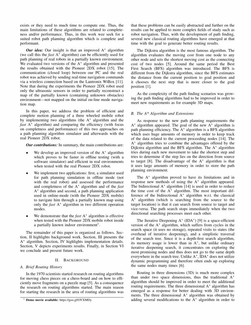
Fig. 2: Second environment map used with the Pioneer 2DX.Initial robot position (R); Final robot destination (D).

Figure 2 depicts a partially known environment. Notethat the rectangles with diagonals lines inside (O1 and O2)depicted in Figure 2 represent unknown obstacles which werepreviously not modeled inside the path planning applicationmap (Java back-end application) depicted in Figure 3. The fastA∗ algorithm was tested on this two maps (with only and O1and then with both O1 and O2) with the real Pioneer 2DXrobot simulator [17] with the goal to find out if the robot candeal with partially known environments. The experiment wasperformed in a room having six by eight meters and by re-modeling it in the steering application depicted in Figure 3.We used for the online experiments the 14 configuration fromTable II (i.e., Heuristic # 8, Diagonals on (D) and FormulaM(x,y)). We decided to use this configuration because it wasthe longest run from our experiments where the Heuristic #number could be increased (8 times) until the search time

(Time [sec]) started to rise again. We leave the experimentswith other settings as a future exercise.

First, an unknown obstacle (i.e., depicted in Figure 2 withO2) was added to the test environment (room) and the pathplanner application (online mode) was ran. Second, anotherunknown obstacle (i.e., depicted in Figure 2 with O2) wasplaced in the same test environment as before. As result thetest environment contained two unknown obstacles (i.e., O1and O2). Finally, for both of this scenarios the runtimes ofthe Pioneer 2DX robot were measured by navigating from theinitial location (depicted in Figure 2 with letter R) to the finallocation (depicted in Figure 2 with letter D). The results ofthese experiments are depicted in Table III.

Note that the obstacles depicted in the Pioneer simu-lator map (Figure 2) are not present in the path plannerapplication—Figure 3. Thus the robot had to deal with thisobstacles in order to reach its target destination which waspreviously given (i.e., denoted with letter D in Figure 3).

R

D

Fig. 3: Environment map available in the path planner. Initialrobot position (R); Final robot destination (D).

Figure 3 presents the map of the room as it was modeledin the steering application—blue map areas/yellow map areasrepresent non passable/passable map areas. Note that this mapdid not contain the obstacles depicted in the map presented inFigure 2 at any time. The 2D map is composed of squareswhich measure in reality 10 by 10 centimeters. We foundout experimentally that larger maps can be also used duringour experiments. We tested the the planning application byrunning the fast A∗ algorithm in two different modes (depictedin Table III with M1 (first mode) and M2 (second mode)), formore details see [16]. Table III shows that first mode is bettersuited with the map depicted in Figure 2 with one obstaclewhereas the second mode is better suited for the map presentedin Figure 2 with both obstacles. The first mode differs fromsecond mode w.r.t. action limiters that are not added to therobot (not used during robot movement) in first mode.

TABLE III: Path planning with the fast A∗ algorithm andtwo running modes

Test run Mode Map Time [sec]1 M1 Figure 2 with 1 obstacle 472 M2 Figure 2 with 1 obstacle 453 M1 Figure 2 with 2 obstacle 614 M2 Figure 2 with 2 obstacle 40

Table III depicts the run-times for the two running modeson two real environments. In column four of Table III weobserve that for the first environment (Figure 2 with oneobstacle) the best run-time (47 seconds) is obtained with M1selected and that for the second environment (Figure 2 withtwo obstacles) the best run-time (40 seconds) is obtained withM2 turned on. Note that in Figure 2 we had two unknownobstacles (i.e., O1 and O2) which were added one after eachother for each of our experiments. When running the fast A∗algorithm on the map depicted in Figure 2 (containing only O1)with M1 the run-time increases w.r.t. M2 because the range ofthe ultrasonic sensors was set tp 50 millimeters. Note that thesensors distance parameter for M1 was set to 50 millimeterswhereas for M2 this value was set to 225 millimeters. Thus,the robot can make decisions earlier or later along the path. Asresult the obstacle depicted in Figure 2 (i.e., O1) is detectedlater as compared to the detection of both obstacles depictedin Figure 2 when the range of the sensors was increased to 225millimeters. Thus, the result is the addition of several recoveryactions needed in order to recuperate the robot and point himto the target destination.

However, when performing path planning with the mapdepicted in Figure 2 with two unknown obstacles using M2the run-time decreases because the range of the ultrasonicsensors was set to 225 millimeters and the result is that theobstacles are detected earlier. This removes additional recoveryactions needed by the robot in order to find a new obstacleavoiding path, thus time is not wasted. We infer (with caution)from these results that the second mode is best suited forenvironments with more unknown obstacles whereas the firstmode is better suited for environments with less unknownobstacles.

VI. CONCLUSION AND FUTURE WORK

In this paper, we evaluated the A∗ algorithm and the fastA∗ algorithm w.r.t. completness and we shown that the fastA∗ algorithm can be successfully used for indoor mobilerobot navigation by using only data collected from ultrasonicsensors. We built two software tools (for offline and onlinealgorithm testing) which helped to tweak the used algorithmsand to take further decisions based on this results. The resultsobtained from comparing the A∗ algorithm and the fast A∗algorithm (Section V-A) indicate a speed-up of two ordersof magnitude w.r.t. the fast A∗ algorithm inside our offlinesimulator. The second mode used with the fast A∗ algorithmis best suited for environments with less unknown obstacleswhereas the first mode is better suited for environments withmore than one unknown obstacles (in our experiments). We areaware that further experiments are need in order to fully claimthe above stated. Additionally, we showed in our experimentsthat the fast A∗ algorithm is complete (finds a path in due

time). We leave the computation of its performance as a futureexercise.

In future we want to further tweak the fast A∗ algorithmand use other algorithms with more complex unknown en-vironments. We want to use more advanced path planningalgorithms and we want to combine input from multiplesensors (i.e., perform fusion of data from several sources)which will give a more precise description of the environment.Furthermore, we want to compute the performance of the usedalgorithms and compared them with each other.

ACKNOWLEDGEMENTS

We want to express our gratitude to the anonymous review-ers for their constructive criticism.

REFERENCES

[1] Amit’s Game Programming Information, http://www.csstudents.stanford.edu/amitp/gameprog.html, accessed on the 28 Jan. 2010.

[2] Aria, ActivMedia Robotics, Inc. Aria Reference Manual 1.1.10, 2002.[3] A∗ algorithm, Available [Online], http://en.wikipedia.org/wiki/A*

search algorithm.[4] Counter-strike video game, Available [Online], https://en.wikipedia.org/

wiki/Counter-Strike, 1999.[5] P. W. Eklund, S. Kirkby, and S. Pollitt, A Dynamic Multi-source

Dijkstras Algorithm for Vehicle Routing, In Proceedings of theConference on Intelligent Information Systems, 1996.

[6] Iterative deepening A∗ Available [Online], https://en.wikipedia.org/wiki/Iterative deepening A*.

[7] L. Jaulin, Path planning using intervals and graphs. Reliable Computing7 (1), 2001.

[8] J. H. Jones, A∗ Tutorial. http://cs.nyu.edu/courses/fall10/G22.2965-001/astartravsales, accessed on the 28 Jan. 2010.

[9] R. Korf, Depth-first Iterative-Deepening: An Optimal Admissible TreeSearch, In Artificial Intelligence 27: 97109, 1985.

[10] K. Konolige, K. Myers, E. Ruspini, and A. Saffiotti, The SAPHIRAarchitecture: a design for autonomy, In Artificial Intelligence BasedMobile Robots: Case Studies of Successful Robot Systems, MIT Press,1998.

[11] Lantronix, WiBox 2100 Quick Start Guide, Available [Online], https://www.lantronix.com/wp-content/uploads/pdf/WiBox QS.pdf, Lantronix,2004.

[12] K. Makanae, and M. Takaki, A∗ Tutorial, Development of the3-Dimensional Urban Spatial Data Model and Application to thePedestrian Navigation System, ITS. 2004.

[13] Minkowski addition, Available [Online], https://en.wikipedia.org/wiki/Minkowski addition.

[14] P. C. Nelson, and A. A. Toptsis, Unidirectional and Bidirectional SearchAlgorithms, 1992.

[15] Pioneer2DX Robot, Available [Online], http://wiki.ros.org/Robots/AMR Pioneer Compatible.

[16] J. Rosel, and P. Iniguez, Path planning using Harmonic Functionsand Probabilistic Cell Decomposition, In Proceedings of the IEEEInternational Conference on Robotics and Automation (ICRA), 2005.

[17] Saphira, Saphira Operations and Programming Manual Version 6.2,Mobile Robots ROBOTICS, 1999.

[18] R. Siegwart, and I. R. Nourbakhsh, Introduction to Autonomous MobileRobots, MIT Press, ISBN: 9780262015356, 2004.

[19] Y. Zhang, L. Wu, and S. Wang, UCAV path planning based onFSCABC, In Information-An International Interdisciplinary Journal,pp. 687692, 2011.