Embed Size (px)
Citation preview
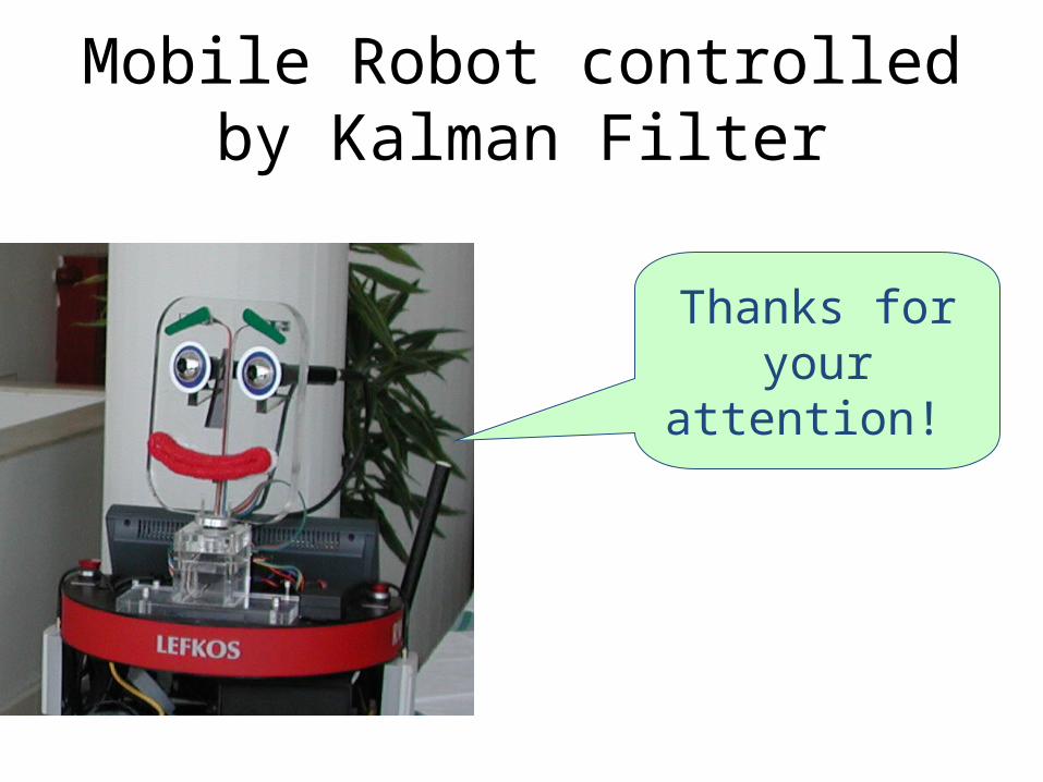
Mobile Robot controlled by Kalman Filter
Thanks for your
attention!
Overview1. What could Kalman Filters be used for?
2. What is a Kalman Filter?
3. Conceptual Overview
4. The Theory of Kalman Filter (only the equations you need to use)
5. Simple Examples
Most Generally: WHAT IS Kalman Filter?
• What is the Kalman Filter?– A technique that can be used to recursively estimate
unobservable quantities called state variables, {xt}, from an observed time series {yt}.
• What is it used for?– Tracking missiles– Extracting lip motion from video– Lots of computer vision applications– Economics– Navigation
Example of Example of estimation estimation
problemproblem
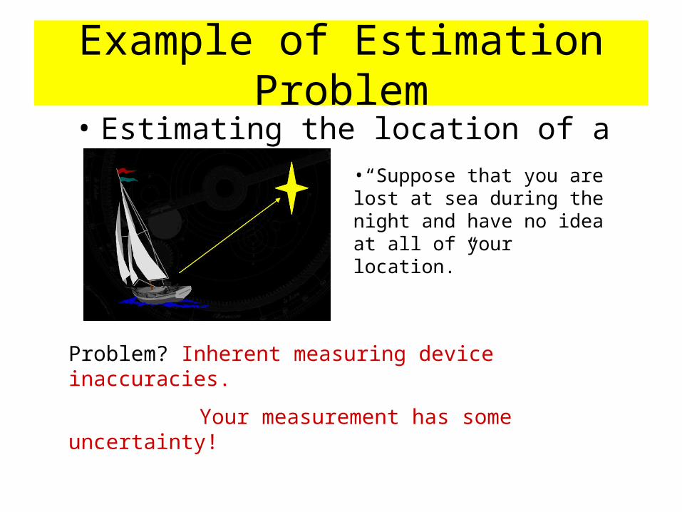
Example of Estimation Problem• Estimating the location of a ship
•“Suppose that you are lost at sea during the night and have no idea at all of your location.”
Problem? Inherent measuring device inaccuracies.
Your measurement has some uncertainty!
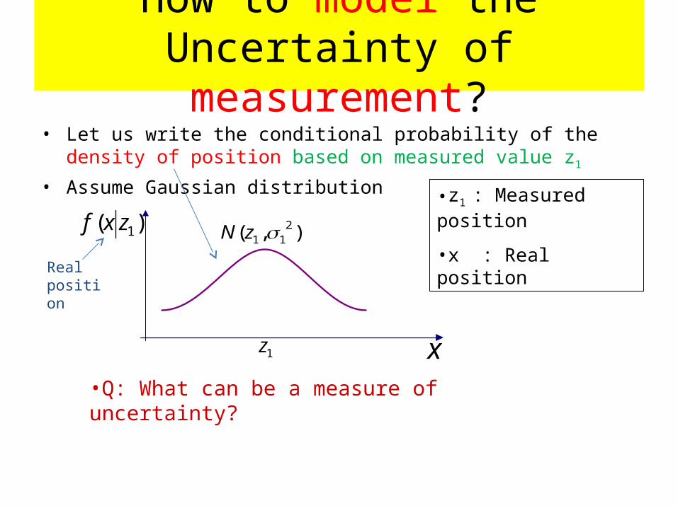
How to model the Uncertainty of measurement?
• Let us write the conditional probability of the density of position based on measured value z1
• Assume Gaussian distribution
),( 211 zN)( 1zxf
x1z
•z1 : Measured position
•x : Real position
•Q: What can be a measure of uncertainty?
Real position
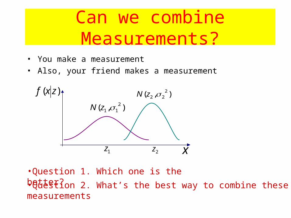
Can we combine Measurements?• You make a measurement• Also, your friend makes a measurement
•Question 1. Which one is the better?
•Question 2. What’s the best way to combine these measurements
),( 211 zN
),( 222 zN)( zxf
x1z 2z
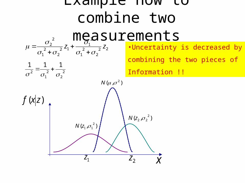
Example how to combine two measurements
),( 211 zN
),( 222 zN
)( zxf
x1z 2z
),( 2N
222
21
21
122
21
22 zz
22
21
2
111
•Uncertainty is decreased by
combining the two pieces of
Information !!
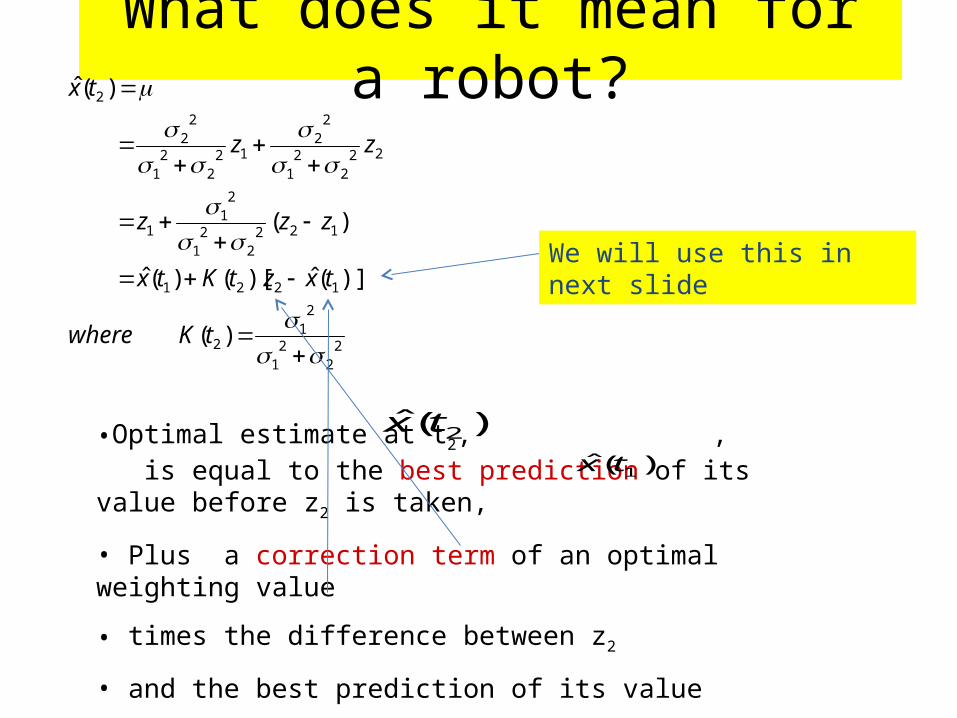
What does it mean for a robot?
22
21
21
2
1221
1222
21
21
1
222
21
22
122
21
22
2
)(
)](ˆ)[()(ˆ
)(
)(ˆ
tKwhere
txztKtx
zzz
zz
tx
)(ˆ 1tx
•Optimal estimate at t2, , is equal to the best prediction of its value before z2 is taken,
• Plus a correction term of an optimal weighting value
• times the difference between z2
• and the best prediction of its value
• before it is actually taken, .
)(ˆ 1tx
)(ˆ 2tx
We will use this in next slide
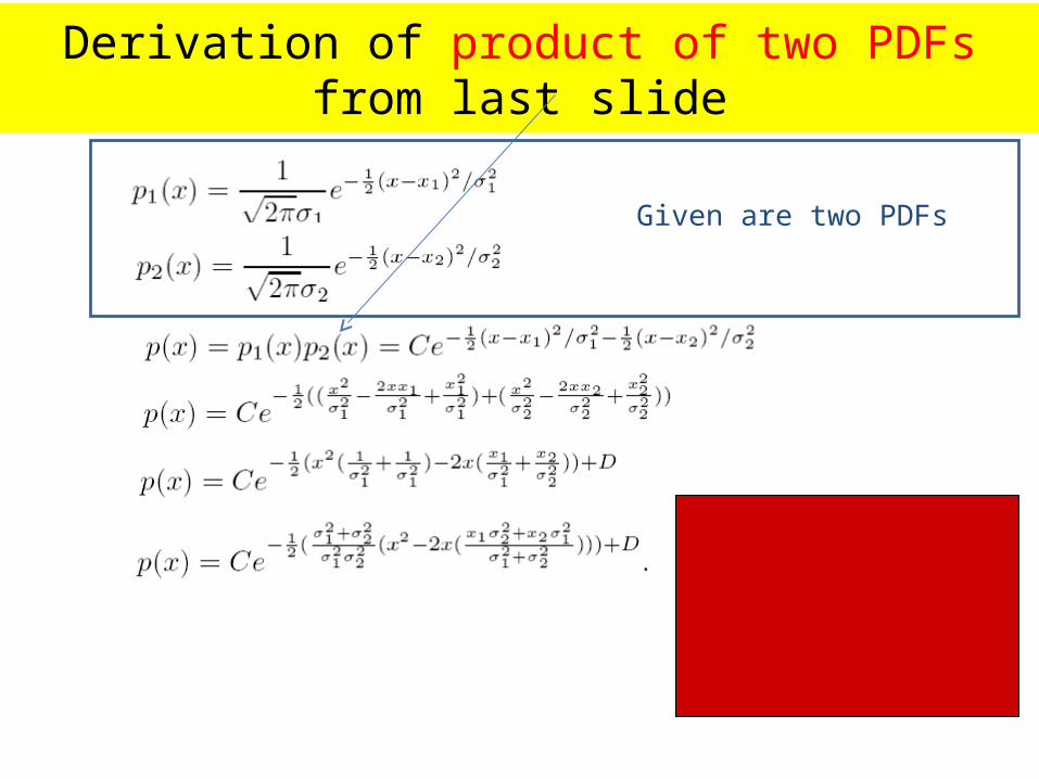
Derivation of product of two PDFs from last slide
Given are two PDFs
What we have discussed
•11
1. Two lectures ago we discussed product of probabilities on discrete examples
2. Last lecture we discussed product of PDFs - Gaussians
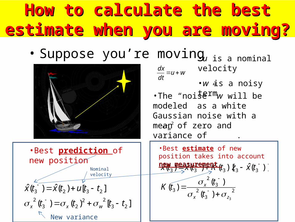
How to calculate the best estimate when How to calculate the best estimate when you are moving?you are moving?
• Suppose you’re movingwu
dt
dx
•u is a nominal velocity
•w is a noisy term
•The “noise” w will be modeled as a white Gaussian noise with a mean of zero and variance of . 2
w
][)()(
][)(ˆ)(ˆ
2322
232
2323
tttt
ttutxtx
wxx
•Best prediction of new position
23
23
2
3
33333
3)(
)()(
)](ˆ)[()(ˆ)(ˆ
zx
x
t
ttK
txztKtxtx
•Best estimate of new position takes into account new measurement new measurement
Nominal velocity
New variance
Summary on models, prediction and correction
• Process Model– Describes how the state changes over time
• Measurement Model– Where you are from what you see !!!
• Predictor-corrector– Predicting the new state and its uncertainty– Correcting with the new measurement

What is a Filter What is a Filter by the way?by the way?
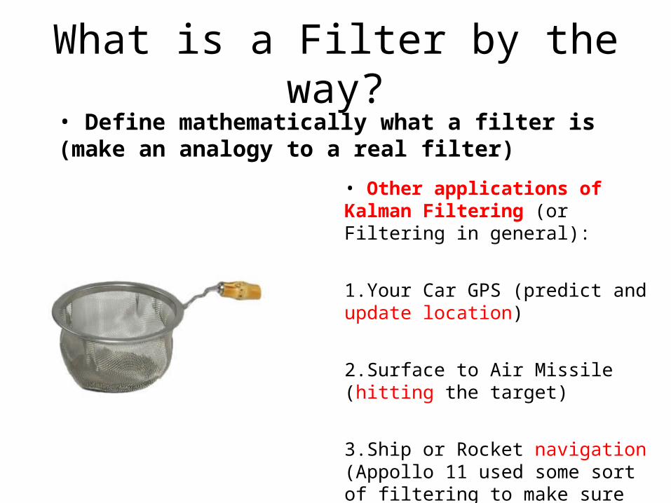
What is a Filter by the way?• Define mathematically what a filter is (make an analogy to a real filter)
• Other applications of Kalman Filtering (or Filtering in general):
1.Your Car GPS (predict and update location)
2.Surface to Air Missile (hitting the target)
3.Ship or Rocket navigation (Appollo 11 used some sort of filtering to make sure it didn’t miss the Moon!)
•16
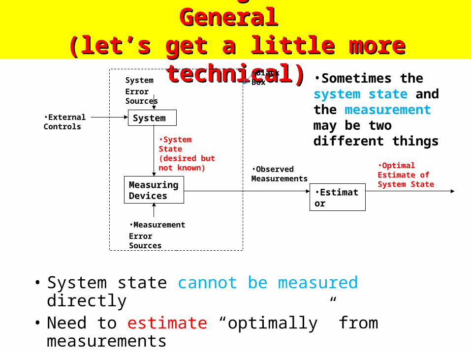
The “filtering Problem” in General The “filtering Problem” in General (let’s get a little more technical)(let’s get a little more technical)
• System state cannot be measured directly• Need to estimate “optimally” from
measurements
Measuring Devices •Estimator
•Measurement
Error Sources
•System State (desired but not known)
•External Controls
•Observed Measurements
•Optimal Estimate of System State
System
Error Sources
System
•Black Box •Sometimes the
system state and the measurement may be two different things

FILTERS IN FILTERS IN MOBILE MOBILE ROBOTSROBOTS
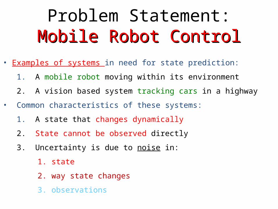
Problem Statement: Mobile Mobile Robot ControlRobot Control
• Examples of systems in need for state prediction:
1. A mobile robot moving within its environment
2. A vision based system tracking cars in a highway
• Common characteristics of these systems:
1. A state that changes dynamically
2. State cannot be observed directly
3. Uncertainty is due to noise in:
1. state
2. way state changes
3. observations
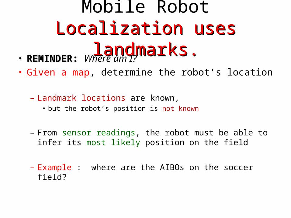
Mobile Robot Localization uses Localization uses landmarks.landmarks.
• REMINDER: REMINDER: Where am I?• Given a map, determine the robot’s location
– Landmark locations are known, • but the robot’s position is not known
– From sensor readings, the robot must be able to infer its most likely position on the field
– Example : where are the AIBOs on the soccer field?
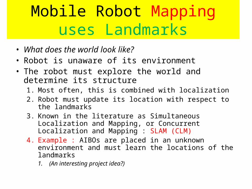
Mobile Robot Mapping uses Landmarks
• What does the world look like?• Robot is unaware of its environment• The robot must explore the world and determine its
structure1. Most often, this is combined with localization2. Robot must update its location with respect to the landmarks3. Known in the literature as Simultaneous Localization and
Mapping, or Concurrent Localization and Mapping : SLAM (CLM)
4. Example : AIBOs are placed in an unknown environment and must learn the locations of the landmarks 1. (An interesting project idea?)
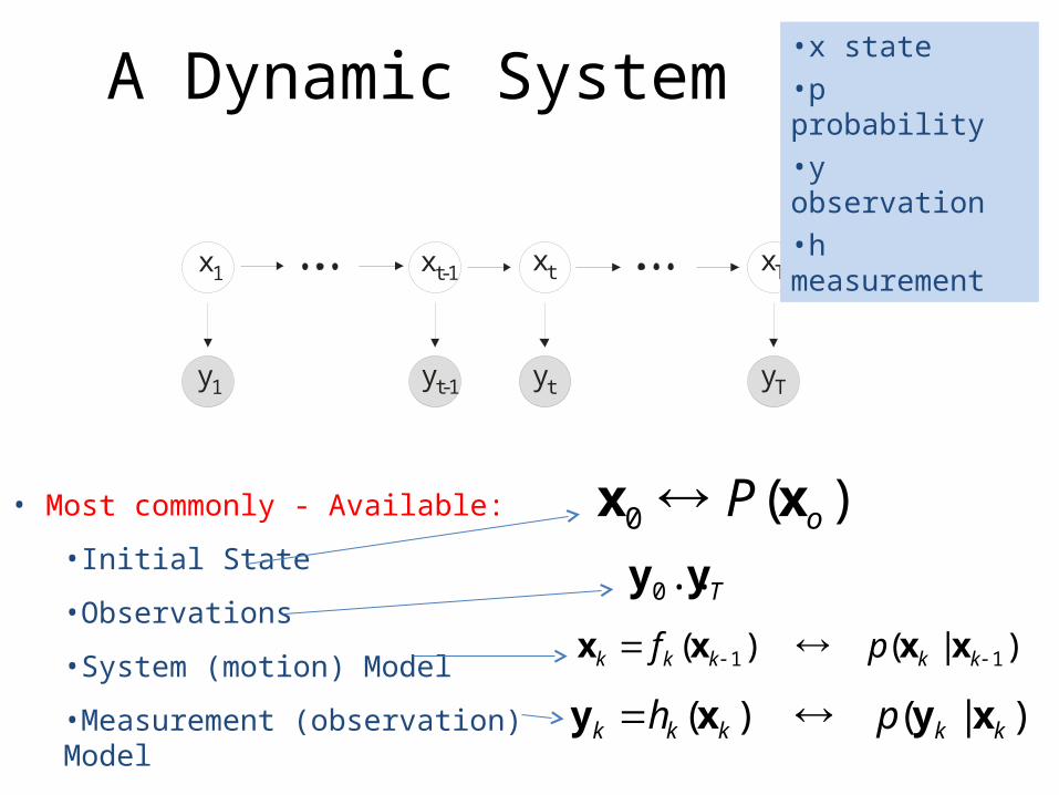
A Dynamic System
xt-1 xt xT
y1 yt-1 yt yT
x1
Tyy ..0
)|( )( 11 kkkkk pf xxxx
)|( )( kkkkk ph xyxy
• Most commonly - Available:
•Initial State
•Observations
•System (motion) Model
•Measurement (observation) Model
)(0 oP xx
•x state•p probability•y observation•h measurement
Filters must be optimal • Filters compute the hidden state from observations
• Filters:– Terminology from signal processing– Can be considered as a data processing algorithm. – Filters are Computer Algorithms or hardware devices (FPGA)
• Filters do classificationFilters do classification
• Classification: Discrete time versus Continuous time Continuous time
Issues:1. Sensor fusion 2. Robustness to noise
Wanted: each filter to be optimal in some sense.
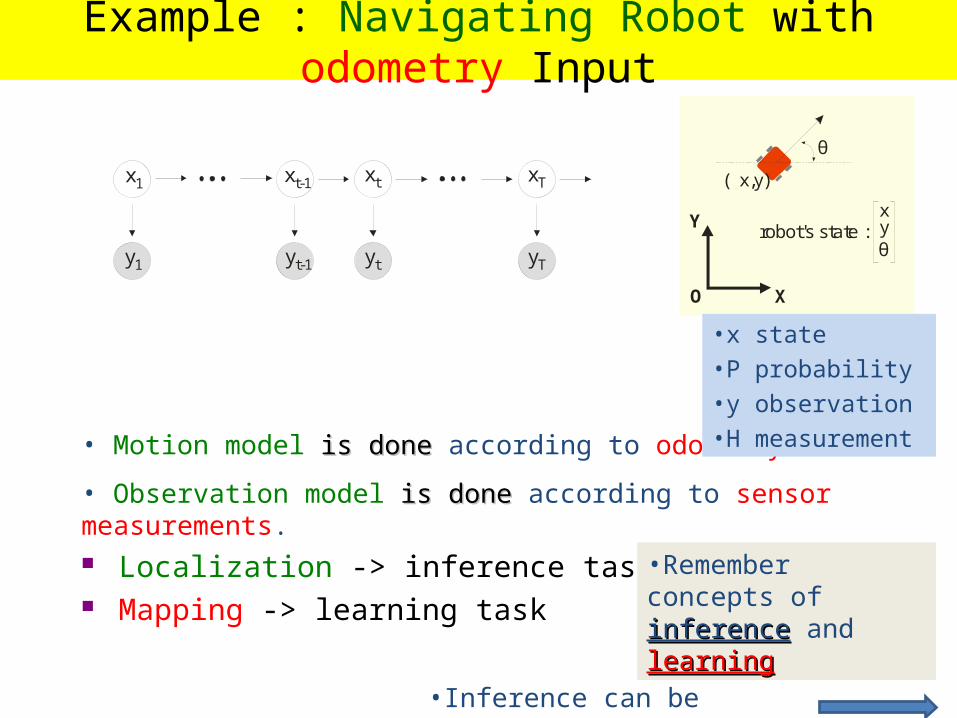
Example : Navigating Robot with odometry Input
xt-1 xt xT
y1 yt-1 yt yT
x1
X
Y
O
θ
( , )x y
robot's state : xyθ
• Motion model is done is done according to odometry.
• Observation model is done is done according to sensor measurements. Localization -> inference task Mapping -> learning task
•x state•P probability•y observation•H measurement
•Remember concepts of inferenceinference and learninglearning
•Inference can be Bayesian
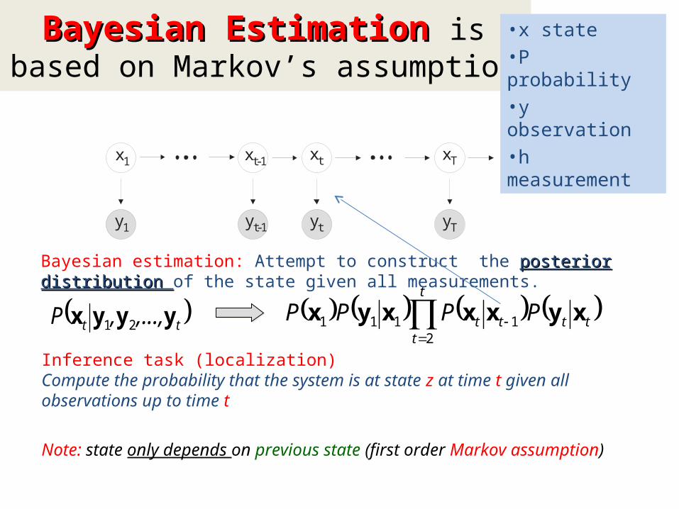
Bayesian Estimation Bayesian Estimation is based on Markov’s assumption
xt-1 xt xT
y1 yt-1 yt yT
x1
t
ttttt PPPP
21111 xyxxxyx tt ,...,,P yyyx 21
Inference task (localization)Compute the probability that the system is at state z at time t given all observations up to time t
Note: state only depends on previous state (first order Markov assumption)
Bayesian estimation: Attempt to construct the posterior distribution posterior distribution of the state given all measurements.
•x state•P probability•y observation•h measurement
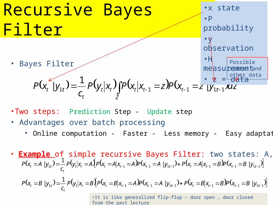
Recursive Bayes Filter
Z
ttttttt
tt dzyzxPzxxPxyPc
yxP 1:111:1 |1
|
1:1111:111:1 ||1
| ttttttttttt
tt yBxPBxBxPyAxPAxBxPBxyPc
yBxP
1:1111:111:1 ||1
| ttttttttttt
tt yBxPBxAxPyAxPAxAxPAxyPc
yAxP
• Bayes Filter
•Two steps: Prediction Step - Update step
• Advantages over batch processing • Online computation - Faster - Less memory - Easy adaptation
• Example of simple recursive Bayes Filter: two states: A,B
•x state•P probability•y observation•H measurement• z = dataPossible
states and other data
•It is like generalized flip-flop – door open , door closed from the past lecture
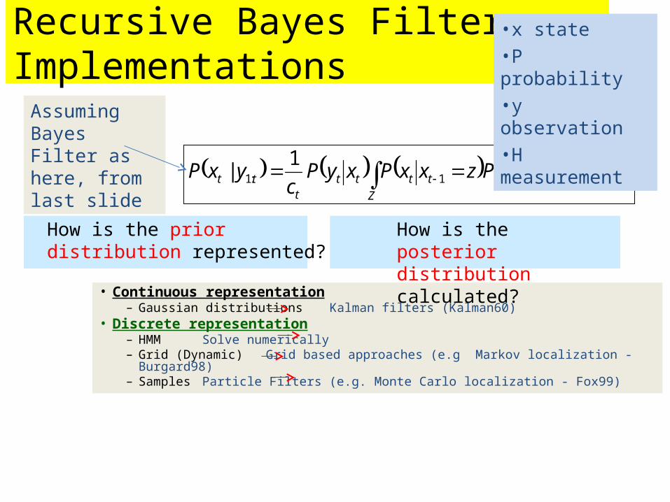
Recursive Bayes FilterImplementations
Z
ttttttt
tt dzyzxPzxxPxyPc
yxP 1:111:1 |1
|
• Continuous representation– Gaussian distributions Kalman filters (Kalman60)
• Discrete representation– HMM Solve numerically – Grid (Dynamic) Grid based approaches (e.g Markov localization -
Burgard98)– Samples Particle Filters (e.g. Monte Carlo localization - Fox99)
How is the prior distribution represented?
How is the posterior distribution calculated?
•x state•P probability•y observation•H measurement
Assuming Bayes Filter as here, from last slide
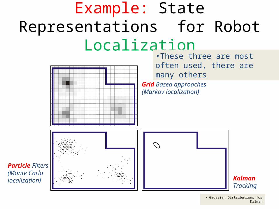
Example: State Representations for Robot Localization
• Gaussian Distributions for Kalman
Grid Based approaches (Markov localization)
Particle Filters (Monte Carlolocalization)
Kalman Tracking
•These three are most often used, there are many others
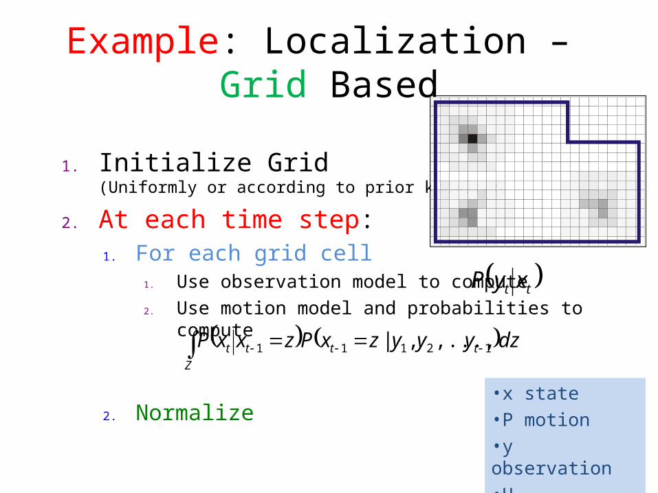
Example: Localization – Grid Based
1. Initialize Grid(Uniformly or according to prior knowledge)
2. At each time step:1. For each grid cell
1. Use observation model to compute2. Use motion model and probabilities to compute
2. Normalize
Z
tttt dzyyyzxPzxxP 12111 ,...,,|
tt xyP
•x state•P motion•y observation•H measurement

Bayesian Bayesian FilterFilter
Why Bayesian Filters are so important?1. Why should you care about Bayesian Filters?
– Robot and environmental state estimation is a fundamental problem in mobile robotics, and in our projects of GuideBot !
2. Nearly all algorithms that exist for spatial reasoning make use of this approach1. If you’re working in mobile robotics, you’ll see it over and
over!2. Very important to understand and appreciate
3. Bayesian Filters are Efficient state estimators– Recursively compute the robot’s current state based on the
previous state of the robot
What is the robot’s state?
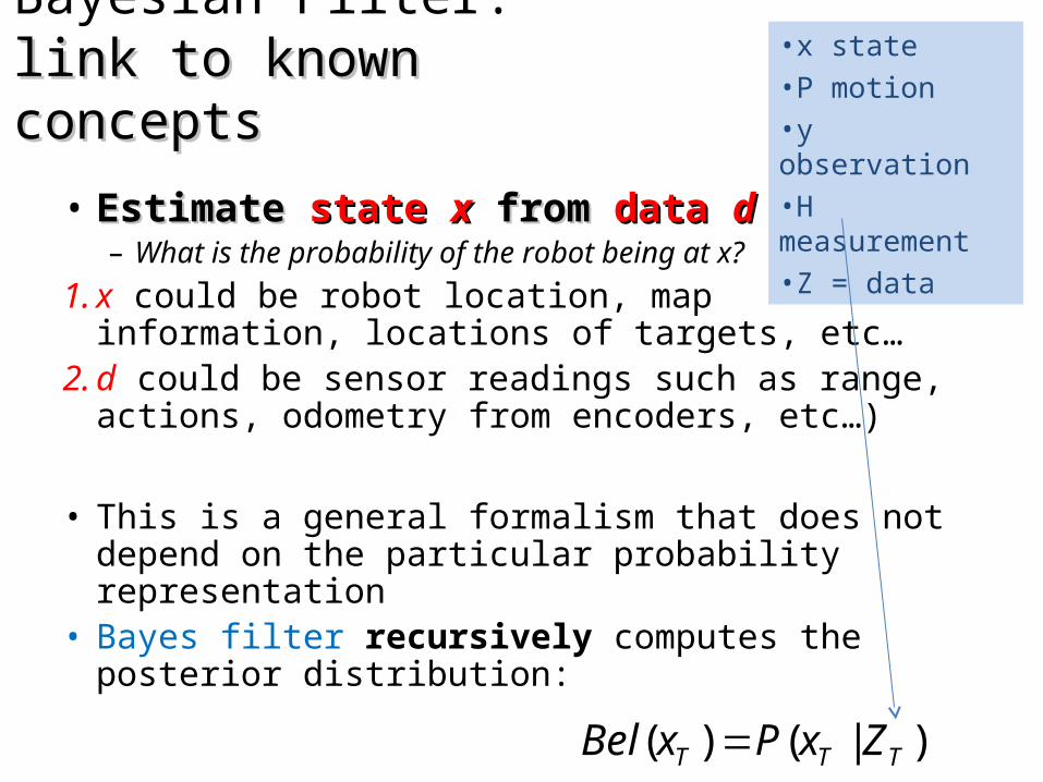
Bayesian Filter: link to known link to known conceptsconcepts
• Estimate Estimate state state xx from from data data dd– What is the probability of the robot being at x?
1. x could be robot location, map information, locations of targets, etc…
2. d could be sensor readings such as range, actions, odometry from encoders, etc…)
• This is a general formalism that does not depend on the particular probability representation
• Bayes filter recursively computes the posterior distribution:
)|()( TTT ZxPxBel
•x state•P motion•y observation•H measurement•Z = data
What is a Posterior What is a Posterior Distribution?Distribution?

Derivation of Derivation of the Bayesian the Bayesian
FilterFilter
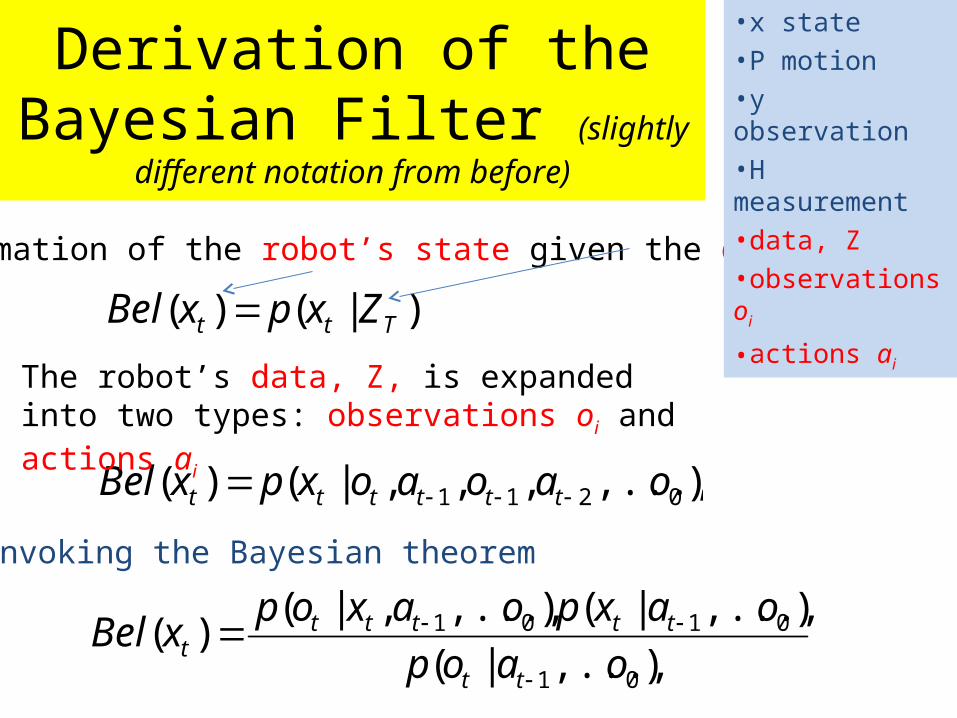
Derivation of the Bayesian Filter (slightly different notation from before)
)|()( Ttt ZxpxBel
),...,,,,|()( 0211 oaoaoxpxBel tttttt
),...,|(
),...,|(),...,,|()(
01
0101
oaop
oaxpoaxopxBel
tt
tttttt
•Estimation of the robot’s state given the data:
The robot’s data, Z, is expanded into two types: observations oi and actions ai
•Invoking the Bayesian theorem
•x state•P motion•y observation•H measurement•data, Z•observations oi
•actions ai
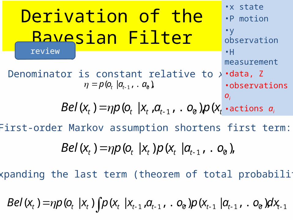
Derivation of the Bayesian Filter
),...,|( 01 aaop tt
),...,|(),...,,|()( 0101 oaxpoaxopxBel tttttt
),...,|()|()( 01 oaxpxopxBel ttttt
1011011 ),...,|(),...,,|()|()( ttttttttt dxoaxpoaxxpxopxBel
Denominator is constant relative to xt
First-order Markov assumption shortens first term:
Expanding the last term (theorem of total probability):
•x state•P motion•y observation•H measurement•data, Z•observations oi
•actions ai
review
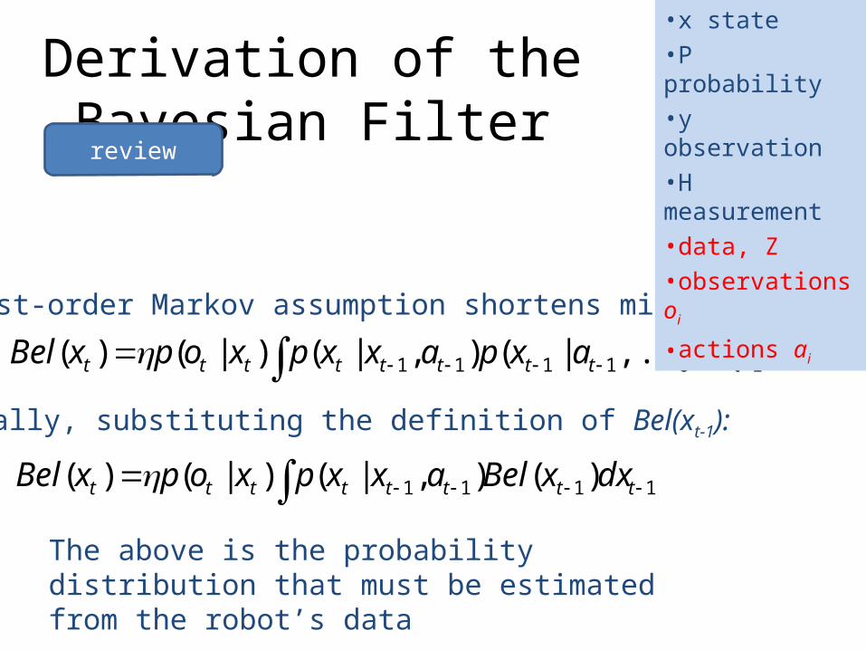
Derivation of the Bayesian Filter
101111 ),...,|(),|()|()( ttttttttt dxoaxpaxxpxopxBel
1111 )(),|()|()( tttttttt dxxBelaxxpxopxBel
First-order Markov assumption shortens middle term:
Finally, substituting the definition of Bel(xt-1):
The above is the probability distribution that must be estimated from the robot’s data
•x state•P probability•y observation•H measurement•data, Z•observations oi
•actions ai
review
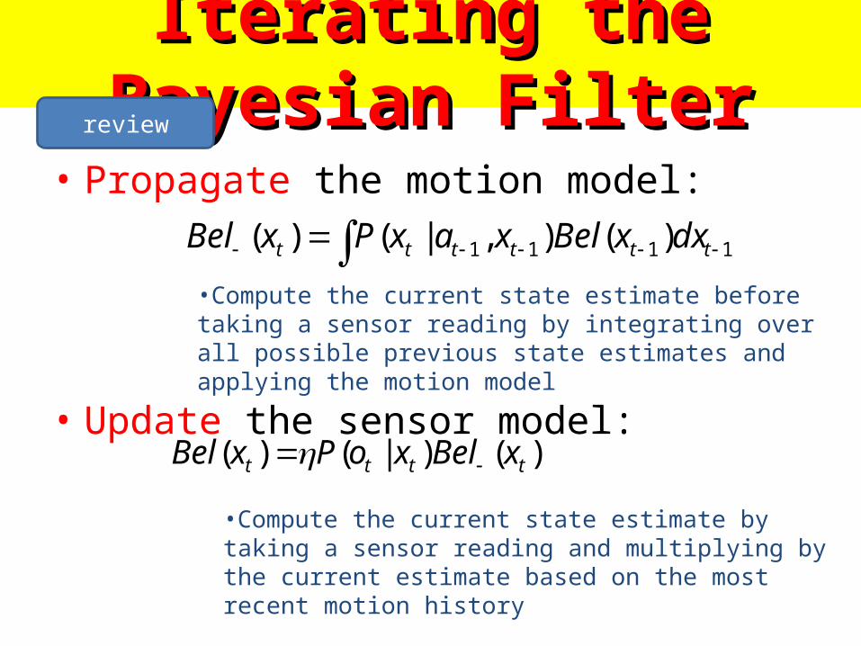
Iterating the Bayesian FilterIterating the Bayesian Filter• Propagate the motion model:
• Update the sensor model:
1111 )(),|()( tttttt dxxBelxaxPxBel
)()|()( tttt xBelxoPxBel
•Compute the current state estimate before taking a sensor reading by integrating over all possible previous state estimates and applying the motion model
•Compute the current state estimate by taking a sensor reading and multiplying by the current estimate based on the most recent motion history
review
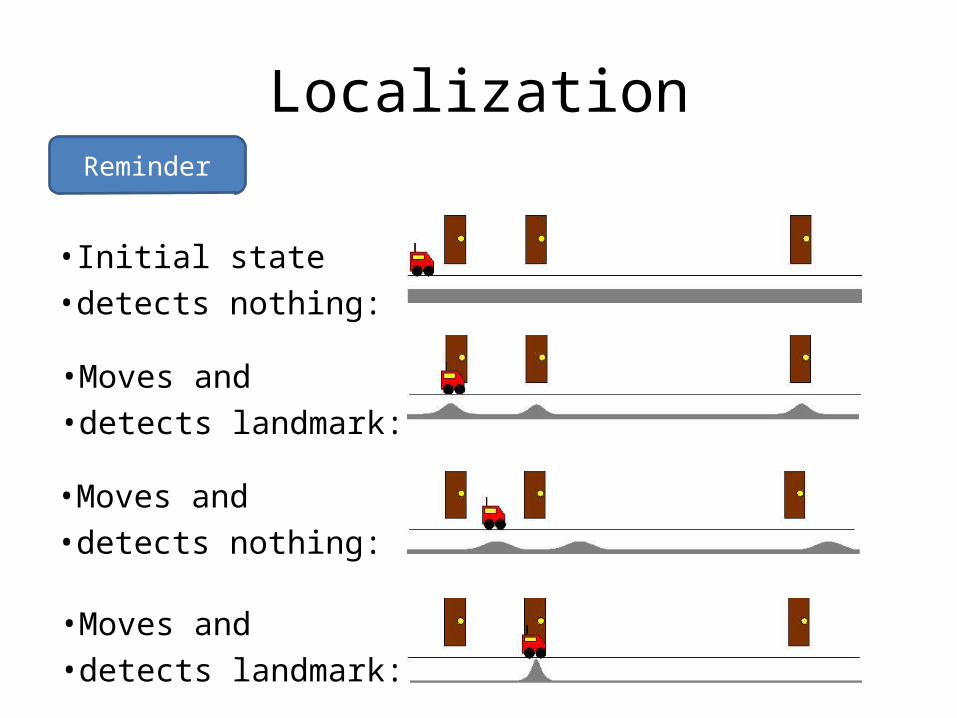
Localization
•Initial state•detects nothing:
•Moves and •detects landmark:
•Moves and •detects nothing:
•Moves and •detects landmark:
Reminder
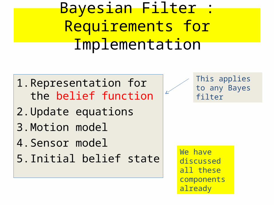
Bayesian Filter : Requirements for Implementation
1. Representation for the belief function
2. Update equations 3. Motion model4. Sensor model5. Initial belief state
This applies to any Bayes filter
We have discussed all these components already
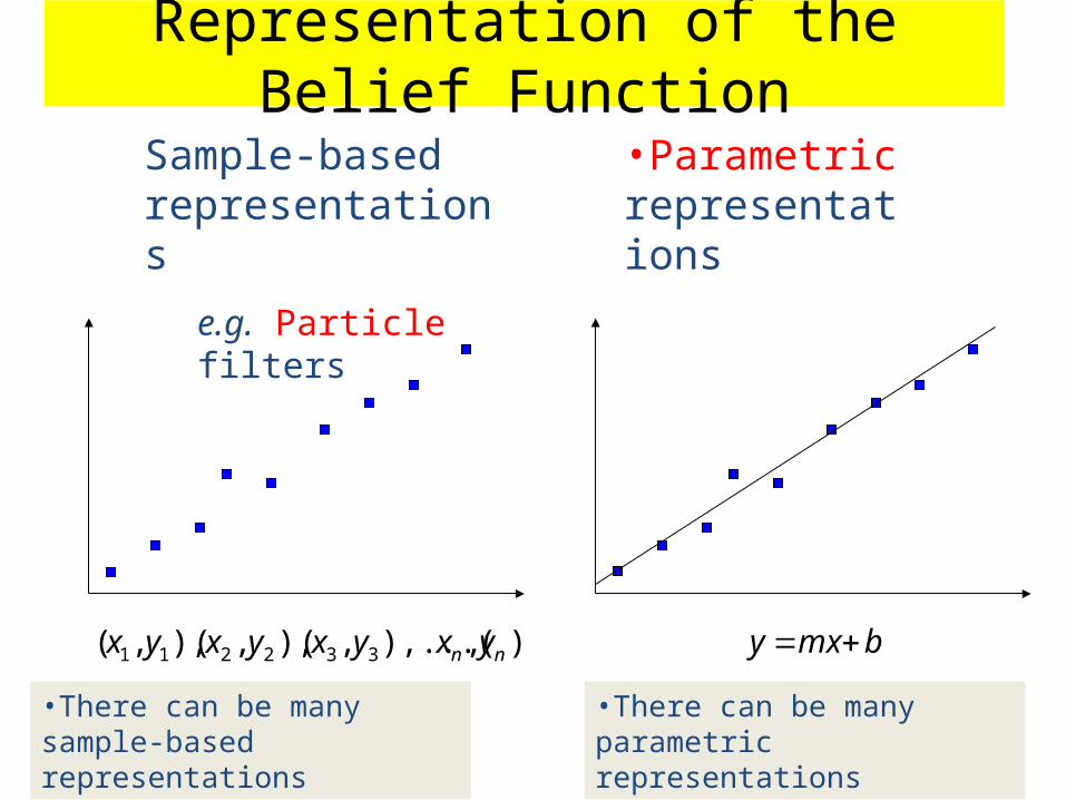
Representation of the Belief Function
),),...(,(),,(),,( 332211 nn yxyxyxyx bmxy
•Parametric representations
Sample-based representations
e.g. Particle filters
•There can be many sample-based representations
•There can be many parametric representations
References• You can find useful materials about HMM from
– CS570 AI Lecture Note(2003)– http://www.idiap.ch/~bengio/– http://speech.chungbuk.ac.kr/~owkwon/
• You can find useful materials about Kalman Filter from – http://www.cs.unc.edu/~welch/kalman– Maybeck, 1979, “Stochastic models, estimation, and
control”– Greg Welch, and Gray Bishop, 2001, “An introduction
to the Kalman Filter”
SourcesPaul E. RybskiHaris Baltzakis
•42