Mobile Positioning Using Wireless Networksemits.esa.int/...RD24-Mobile-positioning-using-wireless-networks.pdf · tions associated with mobile positioning based on available wireless

© DIGITALVISION

Positioning in wireless networks is today mainly used for yellow page services. Yet, itsimportance will grow when emergency call services become mandatory as well as withthe advent of more advanced location-based services and mobile gaming. It is also plausi-ble that future resource management algorithms may rely on position estimation andprediction. In this article, we discuss and illustrate possibilities and fundamental limita-

tions associated with mobile positioning based on available wireless network measurements. Thepossibilities include a sensor fusion approach and model-based filtering, while the fundamental limi-tations provide hard bounds on the accuracy of position estimates, given the information in themeasurements in the most favorable situation. The focus is on illustrating the relation between per-formance requirements, such as those stated by the Federal Communications Commission (FCC),and the available measurements. Specific issues on accuracy limitation in each measurement, suchas synchronization and multipath problems, are only briefly commented upon. A geometrical exam-ple, as well as a realistic example adopted from a cell planning tool, are used for illustration.

MOBILE POSITIONINGVarious location-based services in wireless communication networks depend on mobile posi-tioning. Commercial examples range from low-accuracy methods based on cell identification

Mobile Positioning Using Wireless Networks

[Possibilities and fundamental limitations based on

available wireless network measurements]

[Fredrik Gustafsson and Fredrik Gunnarsson]

1053-5888/05/$20.00©2005IEEE IEEE SIGNAL PROCESSING MAGAZINE [41] JULY 2005

IEEE SIGNAL PROCESSING MAGAZINE [42] JULY 2005

to high-accuracy methods combining wireless network infor-mation and satellite positioning. These methods are typicallynetwork centric, where the position is determined in the net-work and presented to the user via a specific service. Due tologistical reasons, the position is estimated from static snap-shot measurements, possibly provided by the mobile station(MS). Mobile-centric solutions enable the use of sampled tem-poral measurements and motion models to enhance estima-tion accuracy and integrity. Measurements either explicitly orimplicitly relate the MS position to the position of referencepoints (RP) (e.g., positions of radio base stations or satellites)or to the specific behavior of the MS and its surrounding envi-ronment. Measurements are typically directional, such as theangle of arrival (AOA) between MS and RP, or related to rela-tive distances, such as the time of arrival (TOA), time differ-ence of arrival (TDOA), and received signal strength (RSS).The survey articles [1]–[5] provide further information aboutpositioning in wireless networks and associated standardiza-tion. Indoor positioning includes its own specific challengesand is discussed in [6]. Localization based on ultra-wideband(UWB) radios is particularly suitable for limited range posi-tioning, and is discussed in [7]. Another related area is sensorcooperative localization [8], which is integral to sensor net-works positioning.

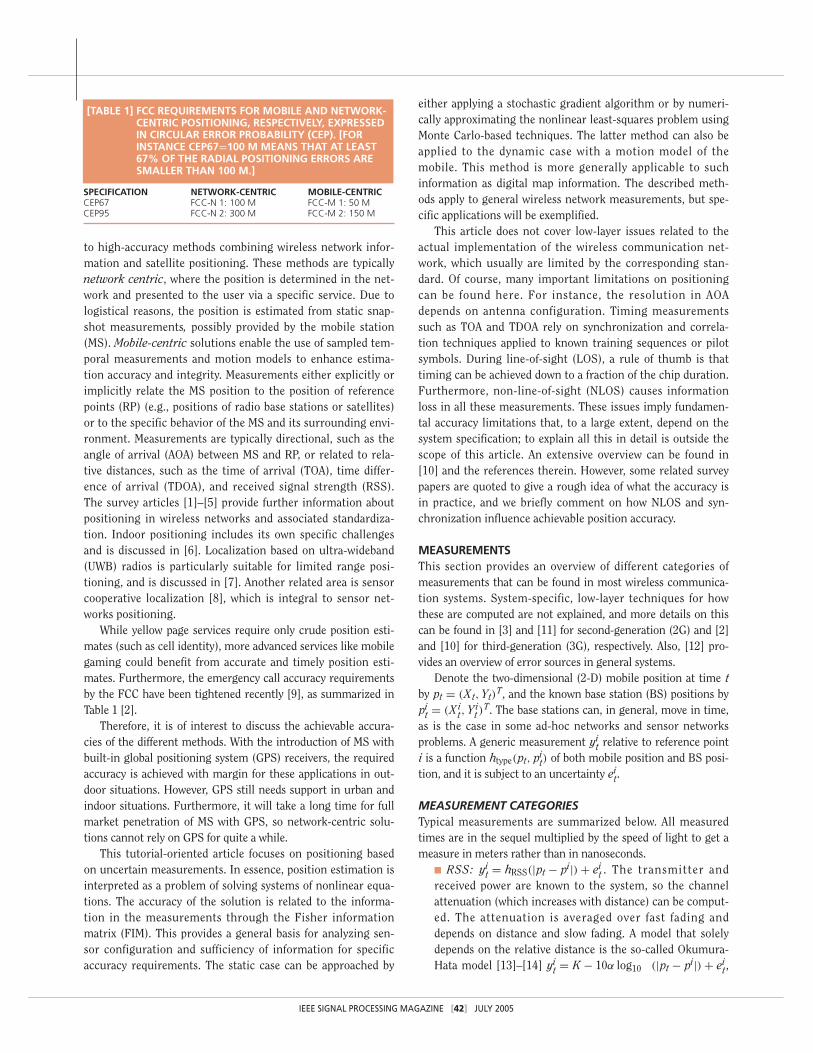
While yellow page services require only crude position esti-mates (such as cell identity), more advanced services like mobilegaming could benefit from accurate and timely position esti-mates. Furthermore, the emergency call accuracy requirementsby the FCC have been tightened recently [9], as summarized inTable 1 [2].

Therefore, it is of interest to discuss the achievable accura-cies of the different methods. With the introduction of MS withbuilt-in global positioning system (GPS) receivers, the requiredaccuracy is achieved with margin for these applications in out-door situations. However, GPS still needs support in urban andindoor situations. Furthermore, it will take a long time for fullmarket penetration of MS with GPS, so network-centric solu-tions cannot rely on GPS for quite a while.

This tutorial-oriented article focuses on positioning basedon uncertain measurements. In essence, position estimation isinterpreted as a problem of solving systems of nonlinear equa-tions. The accuracy of the solution is related to the informa-tion in the measurements through the Fisher informationmatrix (FIM). This provides a general basis for analyzing sen-sor configuration and sufficiency of information for specificaccuracy requirements. The static case can be approached by

either applying a stochastic gradient algorithm or by numeri-cally approximating the nonlinear least-squares problem usingMonte Carlo-based techniques. The latter method can also beapplied to the dynamic case with a motion model of themobile. This method is more generally applicable to suchinformation as digital map information. The described meth-ods apply to general wireless network measurements, but spe-cific applications will be exemplified.

This article does not cover low-layer issues related to theactual implementation of the wireless communication net-work, which usually are limited by the corresponding stan-dard. Of course, many important limitations on positioningcan be found here. For instance, the resolution in AOAdepends on antenna configuration. Timing measurementssuch as TOA and TDOA rely on synchronization and correla-tion techniques applied to known training sequences or pilotsymbols. During line-of-sight (LOS), a rule of thumb is thattiming can be achieved down to a fraction of the chip duration.Furthermore, non-line-of-sight (NLOS) causes informationloss in all these measurements. These issues imply fundamen-tal accuracy limitations that, to a large extent, depend on thesystem specification; to explain all this in detail is outside thescope of this article. An extensive overview can be found in[10] and the references therein. However, some related surveypapers are quoted to give a rough idea of what the accuracy isin practice, and we briefly comment on how NLOS and syn-chronization influence achievable position accuracy.

MEASUREMENTSThis section provides an overview of different categories ofmeasurements that can be found in most wireless communica-tion systems. System-specific, low-layer techniques for howthese are computed are not explained, and more details on thiscan be found in [3] and [11] for second-generation (2G) and [2]and [10] for third-generation (3G), respectively. Also, [12] pro-vides an overview of error sources in general systems.

Denote the two-dimensional (2-D) mobile position at time tby pt = (Xt, Yt)

T, and the known base station (BS) positions bypi

t = (Xit, Yi

t)T. The base stations can, in general, move in time,

as is the case in some ad-hoc networks and sensor networksproblems. A generic measurement yi

t relative to reference pointi is a function htype(pt, pi

t) of both mobile position and BS posi-tion, and it is subject to an uncertainty ei

t.

MEASUREMENT CATEGORIESTypical measurements are summarized below. All measuredtimes are in the sequel multiplied by the speed of light to get ameasure in meters rather than in nanoseconds.

■ RSS: yit = hRSS(|pt − pi|) + ei

t . The transmitter andreceived power are known to the system, so the channelattenuation (which increases with distance) can be comput-ed. The attenuation is averaged over fast fading anddepends on distance and slow fading. A model that solelydepends on the relative distance is the so-called Okumura-Hata model [13]–[14] yi

t = K − 10α log10 (|pt − pi|) + eit,

SPECIFICATION NETWORK-CENTRIC MOBILE-CENTRIC CEP67 FCC-N 1: 100 M FCC-M 1: 50 M CEP95 FCC-N 2: 300 M FCC-M 2: 150 M

[TABLE 1] FCC REQUIREMENTS FOR MOBILE AND NETWORK-CENTRIC POSITIONING, RESPECTIVELY, EXPRESSEDIN CIRCULAR ERROR PROBABILITY (CEP). [FORINSTANCE CEP67=100 M MEANS THAT AT LEAST67% OF THE RADIAL POSITIONING ERRORS ARESMALLER THAN 100 M.]


where std(eit) ≈ 4 − 12 dB depending on the environment

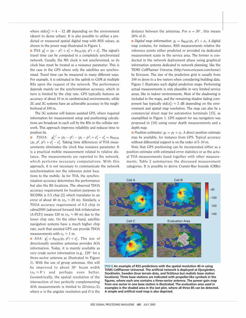
(desert to dense urban). It is also possible to utilize a pre-dicted or measured spatial digital map with RSS values, asshown in the power map illustrated in Figure 1.■ TOA: yi

t = |pt − pi| + eit = hTOA(pt, pi) + ei

t. The signal’stravel time can be computed in a completely synchronizednetwork. Usually, the MS clock is not synchronized, so itsclock bias must be treated as a nuisance parameter. This isthe case in the GPS where only the satellites are synchro-nized. Travel time can be measured in many different ways.For example, it is estimated in the uplink to GSM at multipleBSs upon the request of the network. The performancedepends mainly on the synchronization accuracy, which inturn is limited by the chip rate. GPS typically features anaccuracy of about 10 m in unobstructed environments, while2G and 3G systems have an achievable accuracy in the neigh-borhood of 100 m.

The 3G systems will feature assisted GPS, where requiredinformation for measurement setup and positioning calcula-tions are broadcast in each cell by the BSs in the cellular net-work. This approach improves reliability and reduces time toposition fix.■ TDOA: yi, j

t = |pt − pi| − |pt − pj| + eit − ei

t = hTDOA

(pt, pi, pj) + eit − ei

t. Taking time differences of TOA meas-urements eliminates the clock bias nuisance parameter. Itis a practical mobile measurement related to relative dis-tance. The measurements are reported to the network,which performs necessary computations. With thisapproach, it is not necessary to communicate the networksynchronization nor the reference point loca-tions to the mobile. As for TOA, the synchro-nization accuracy determines the performancebut also the BS locations. The observed TDOAaccuracy requirement for location purposes inWCDMA is 0.5 chip [2] which translates to anerror of about 40 m (σe ≈ 20 m). Similarly, aTDOA accuracy requirement of 0.5 chip incdma2000 [advanced forward link trilateration(A-FLT)] means 120 m (σe ≈ 60 m) due to thelower chip rate. On the other hand, satellitenavigation systems have a much higher chiprate, such that assisted GPS can provide TDOAmeasurements with σe ≈ 1 m.■ AOA: yi

t = hAOA(pt, pi) + eit . The use of

directionally sensitive antennas provides AOAinformation. Today, it is mainly available asvery crude sector information (e.g., 120◦ for athree-sector antenna as illustrated in Figure1). With the use of group antennas, this willbe improved to about 30◦ beam width(σe ≈ 8◦ ) and perhaps even better.Geometrically, the spatial resolution of theintersection of two perfectly complementingAOA measurements is limited to 2D sin(α/2),where α is the angular resolution and D is the

distance between the antennas. For α = 30◦ , this means36% of D.■ Digital map information: yt = hMAP(pt, pi) + et. A digitalmap contains, for instance, RSS measurements relative thereference points either predicted or provided via dedicatedmeasurement scans in the service area. The former is con-ducted in the network deployment phase using graphicalinformation systems dedicated to network planning, like theTEMS CellPlanner Universa (http://www.ericsson.com/tems/)by Ericsson. The size of the prediction grid is usually from100 m down to a few meters when considering building data.Figure 1 illustrates such digital prediction maps. Performingactual measurements is only plausible in very limited serviceareas, like in indoor environments. Most of the shadowing isincluded in the maps, and the remaining shadow fading com-ponent has typically std(ei

t) ≈ 3 dB depending on the envi-ronment and spatial map resolution. The map can also be acommercial street map for automotive terminals [15], asexamplified in Figure 1. GPS support for sea navigation wasproposed in [16] using sonar depth measurements and adepth map. ■ Position estimates: yt = pt + et. A direct position estimatemay be available, for instance from GPS. Typical accuracywithout differential support is on the order of 5–10 m. Note that GPS positioning can be incorporated either as a

position estimate with estimated error statistics or as the actu-al TOA measurements fused together with other measure-ments. Table 2 summarizes the discussed measurementcategories. It is possible to derive Cramér-Rao bounds (CRBs)

[FIG1] An example of RSS predictions with the spatial resolution 40 m usingTEMS CellPlanner Universal. The artificial network is deployed at Djurgården,Stockholm, Sweden (true terrain data, and fictitious but realistic base stationlocations). Three base stations are indicated with propeller-like symbols in thefigures, where each one contains a three-sector antenna. The power gain mapfrom one sector in one base station is illustrated. The evaluation area used inexamples is the shaded area in the last plot, where all three BS can be detected.A simple and artifical road map is also depicted.

Cell A Cell B

−140

−120

−100

−80

Cell C Evaluation Area


for the accuracy in each category as a function of system andenvironment parameters (see [7] for some examples). However,our starting point is to use available information in a networkand determine the accuracy of positioning based on this infor-mation. That is, the noise standard deviation values in paran-theses indicate values used in numerical evaluations andrepresent favorable situations with essentially LOS measure-ments. For more detailed discussions regarding measurementaccuracies for TOA/TDOA, see [17]–[20]; for AOA, see [21]; andfor RSS, see [22] and [23]. Note that the quality of the sensorinformation depends not only on the noise variance but alsoon the size and variation in h(p). This is discussed in a latersection on performance bounds.

ERROR MODELSThe accuracy levels indicated in Table 2 are based on severalassumptions. First, the timing measurements are based onsynchronization techniques. In GSM for instance, a 26-bknown training sequence in each burst is found by correla-tion. The bit duration is about 554 m, but using continuoustime techniques, time synchronization down to a fraction (say100 m) is possible. Similar figures hold for the 3G standarduniversal mobile telecommunications system (UMTS), wherethe travel time is estimated using the first detected ray in theRAKE algorithm from the known pilot symbols. The comput-ed time estimates are assumed to be unbiased, with a standarddeviation σ . In many cases, a Gaussian distribution can bemotivated by asymptotic arguments or the central limit theo-rem, so we can assume

pE(et) = N(0, σ 2), (1a)

where N(0, σ 2) is short-hand notation for the Gaussian proba-bility density function (pdf) pE(et) = (2πσ 2)−1/2 e−(e2

t /2σ 2) . Ifthis is not the case, the Gaussian distribution is the leastinformative distribution for a given variance [24], so the lowerbounds to be computed still hold for estimation and filteringalgorithms based on the Gaussian assumption. However, someof the algorithms in the following sections can make use of anypdf for et, thus reducing the attainable lower bounds.

An important assumption for all time measurements is LOS.In an NLOS situation, the time estimate will get a positive biasµ and probably another (larger) variance

pE(et) = N(µ, σ 2NLOS). (1b)

The problem here is that we cannot easily detect NLOS. Onesolution is to use robust algorithms. Another approach is tomodel the error distribution with a mixture, for instance thetwo-mode Gaussian mixture

pE(et) = αN(0, σ 2LOS) + (1 − α)N(µ, σ 2

NLOS), (1c)

where (α, µ, σLOS, σNLOS) are free parameters in the distribu-tion. Here, et falls in the LOS distribution with probability α andthe NLOS distribution with probability 1 − α. Algorithms basedon this distribution will automatically be more robust than algo-rithms that do not model NLOS.

Only TOA and TDOA are discussed above, but similar mix-tures are suitable to use also for AOA, where NLOS againincreases variance.

Another important aspect of the dynamic case with temporalmeasurements is that TOA, TDOA, and AOA measurements arehighly correlated in time. To use these measurements in a filter,the filter update rate should be matched to their coherence time.

STATIC CASEIn the sequel, all available measurements at time t are col-lected in the vector yt, which is related to the mobile posi-tion pt by yt = h(pt) + et. The BS position is from now onimplicit in h(pt). That is, the vector yt can consist of any

combination of informationin Table 2, and its size canchange over time.

In the static case, there isno assumption of temporalcorrelation of the position, sothe position vector is asequence of uncorrelatedparameters estimated in asnap-shot manner. Knowledgeof measurement error distri-butions can improve the per-formance, and Cramér-Rao

lower bounds (CRLBs) serve as fundamental performance limits.

ESTIMATION CRITERIAThe general positioning challenge is to find the position thatminimizes a given norm of the difference of actual measure-ments and the measurement model. Using the minimizingargument notation for a general loss function V(p), we have

p = arg minp

V(p) = arg minp

‖yt − h(p)‖. (2)

The most common choices of norms are discussed below andsummarized in Table 3.

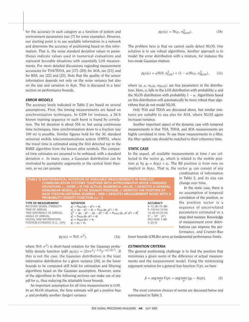
TYPE OF MEASUREMENT NOTATION ACCURACYRECEIVED SIGNAL STRENGTH yi

t = hRSS(|pt − pi|) + eit 4–12 dB (10 dB)

TIME OF ARRIVAL yit = |pt − pi| + ei

t = hTOA(pt, pi) + eit 5–100 M (14 M)

TIME DIFFERENCE OF ARRIVAL yi,jt = |pt − pi| − |pt − pj| + eij

t = hTDOA(pt, pi, pj) + eijt 10–60 M (20 M)

ANGLE OF ARRIVAL yit = hAOA(pt, pi) + ei

t 5o − 10o (6o)

DIGITAL MAP INFORMATION yt = hMAP(pt) + et (RSS MAP, 3 dB) POSITION ESTIMATES (E.G., GPS) yt = pt + et 5–20 M

[TABLE 2] MATHEMATICAL NOTATION OF AVAILABLE MEASUREMENTS IN WIRELESSCOMMUNICATION SYSTEMS TOGETHER WITH APPROXIMATIVE NOISE STANDARDDEVIATIONS σe. [HERE y IS THE ACTUAL NUMERICAL VALUE, h DENOTES A GENERALNONLINEAR MODEL, pt IS THE SOUGHT POSITION, pi DENOTES THE POSITION OFBASE STATION/ANTENNA NUMBER i AND e DENOTES MEASUREMENT NOISE WITH APROBABILITY DENSITY FUNCTION pE(·).]


Table 3 starts withthe nonlinear least-squares criterion. In astochastic settingwhere the measure-ments are subject to astochastic unknownerror et , optimizingthe 2-norm is the best approach ifthe errors are independent, identi-cally distributed Gaussian vari-ables; that is, pE(et) = N(0, σ 2

e I) .If there is a spatial correlation, orif the measurements are of differ-ent quality over time or for differ-ent sensors, improvements are possible. In these cases whereCov(et) = Rt, the weighted NLS is preferred. Further, with agiven error probability distribution pE(e), the maximumlikelihood (ML) approach provides an efficient estimator. Inthe special case of a Gaussian error distribution with posi-tion-dependent covariance pE(et) = N(0, R(pt)), the ML cri-terion is similar to the WNLS criterion, but with the termln det Rt(p). This term prevents the selection of positionswith large uncertainty (large R(pt)), which could be the casewith WNLS.

POSITION ESTIMATIONIn the general case, there is no closed-form solution to (2).One exception is an interesting reformulation of the nonlinearleast-squares problem. It is demonstrated in [25] that byincluding an auxiliary parameter for the absolute distancefrom the MS to an arbitrary reference BS, the NLS problemcan be rewritten as a linear least-squares problem where thereis an additional constraint on the position and the auxiliaryparameter. In this manner, there are no local minima in theloss function. See [5] for a nice summary of explicit least-squares formulations.

In the general case, however, a numerical search methodis needed. As in any estimation algorithm, the classicalchoice is between a gradient and Gauss-Newton algorithm[26]. The basic forms are given in Table 4. These local searchalgorithms generally require good initialization; otherwise,the risk is to reach a local minimum in the loss functionV(p). The least-squares formulation above may provide anadequate initialization. Today, simulation-based optimiza-tion techniques may provide an alternative. For furtherillustrations on computing the ML estimate for TDOA meas-urements, see [27] and [28].

FUNDAMENTAL PERFORMANCE BOUNDSThe FIM provides a fundamental estimation limit for unbiasedestimators referred to as the CRLB [29]. This bound has beenanalyzed thoroughly in the literature, primarily for AOA, TOA,and TDOA [18], [30]–[34], but also for RSS [23], [35] and withspecific attention to the impact from NLOS [36], [37].

The 2 × 2 FIM J(p) is defined as

J(p)=E(∇T

p ln pE(y − h(p))∇p ln pE(y − h(p)))

(3a)

∇p ln pE(y−h(p))=(

d ln pE(y−h(p))dX

d ln pE(y−h(p))dY

),

(3b)

where p = (X, Y) is the 2-D position vector and pE(y − h(p))the likelihood given the error distribution.

In the case of Gaussian measurement errorspE(e) = N(0, R(p)), the FIM equals

J(p) =HT(p)R(p)−1 H(p), (4a)

H(p) =∇ph(p). (4b)

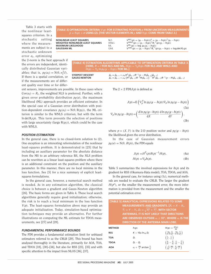
Table 5 summarizes the involved expressions for h(p) and itsgradient for RSS (Okumura-Hata model), TOA, TDOA, and AOA.

In the general case, for instance using (1c), numerical meth-ods are needed to evaluate the CRLB. The larger the gradientH(po), or the smaller the measurement error, the more infor-mation is provided from the measurement and the smaller thepotential estimation error.

NONLINEAR LEAST SQUARES NLS VNLS(p) = ‖yt − h(p))‖2 = (yt − h(p))T (yt − h(p))

WEIGHTED NONLINEAR LEAST SQUARES WNLS VWNLS(p) = (yt − h(p))T R−1t (p)(yt − h(p))

MAXIMUM LIKELIHOOD ML VML(p) = log pE(yt − h(p))

GAUSSIAN ML GML VGML(p) = (yt − h(p))T R−1t (p)(yt − h(p)) + log det Rt(p)

[TABLE 3] OPTIMIZATION CRITERIA V(p) FOR ESTIMATING POSITION p FROM UNCERTAIN MEASUREMENTSy = h(p) + e USING (2). [THE VECTOR ELEMENTS IN y AND h(p) COME FROM TABLE 2.]

STEEPEST DESCENT pk = pk−1 + µkHT (pk−1)R−1(y − H(pk−1)pk−1)

GAUSS-NEWTON pk = pk−1 + µk(HT (pk−1)R−1H(pk−1)

)−1 HT (pk−1)R−1(y − H(pk−1)pk−1)

[TABLE 4] ESTIMATION ALGORITHMS APPLICABLE TO OPTIMIZATION CRITERIA IN TABLE 3.[HERE, R = I FOR NLS AND ML, H(p) = ∇ph(p) FOR NLS AND WNLS ANDH(p) = ∇p ln pE(y − h(p)) FOR ML.]

METHOD h(p) H(p) = dh(p)

dp

RSS K + 10α ln10 Di

(10αln 10

Xi

D2i, 10α

ln 10Yi

D2i

)

TOA Di

(XiDi

, YiDi

)

TDOA Di − Dj

(XiDi

− Xj

Dj, Yi

Di− Yj

Dj

)

AOA αi + 180π

arctan Yi

Xi

(−Yi

D2i

180π

, Xi

D2i

180π

)

[TABLE 5] ANALYTICAL EXPRESSIONS RELATED TO SOME

MEASUREMENTS AND GRADIENTS. [Xi = X − Xi ,

Yi = Y − Yi , Di =√

X2i + Y2

i . WITH SECTOR

ANTENNAS, IT IS NOT LIKELY THAT DIRECTIONS

ARE OBSERVED OUTSIDE αi ± 90o, WHERE αi IS THE

DIRECTION OF THE ANTENNA MAIN LOBE.


Information is additive, so if two measurements are inde-pendent, the corresponding information matrices can be added.This is easily seen from (4a) for HT = (HT

1 , HT2 ) and R being

block diagonal, in which case we can write J = J1 + J2 .Plausible approximate scalar information measures are the traceof the FIM and the smallest eigenvalue of FIM

J tr(p) �= tr J(p), Jmin(p) �= min eig J(p). (5)

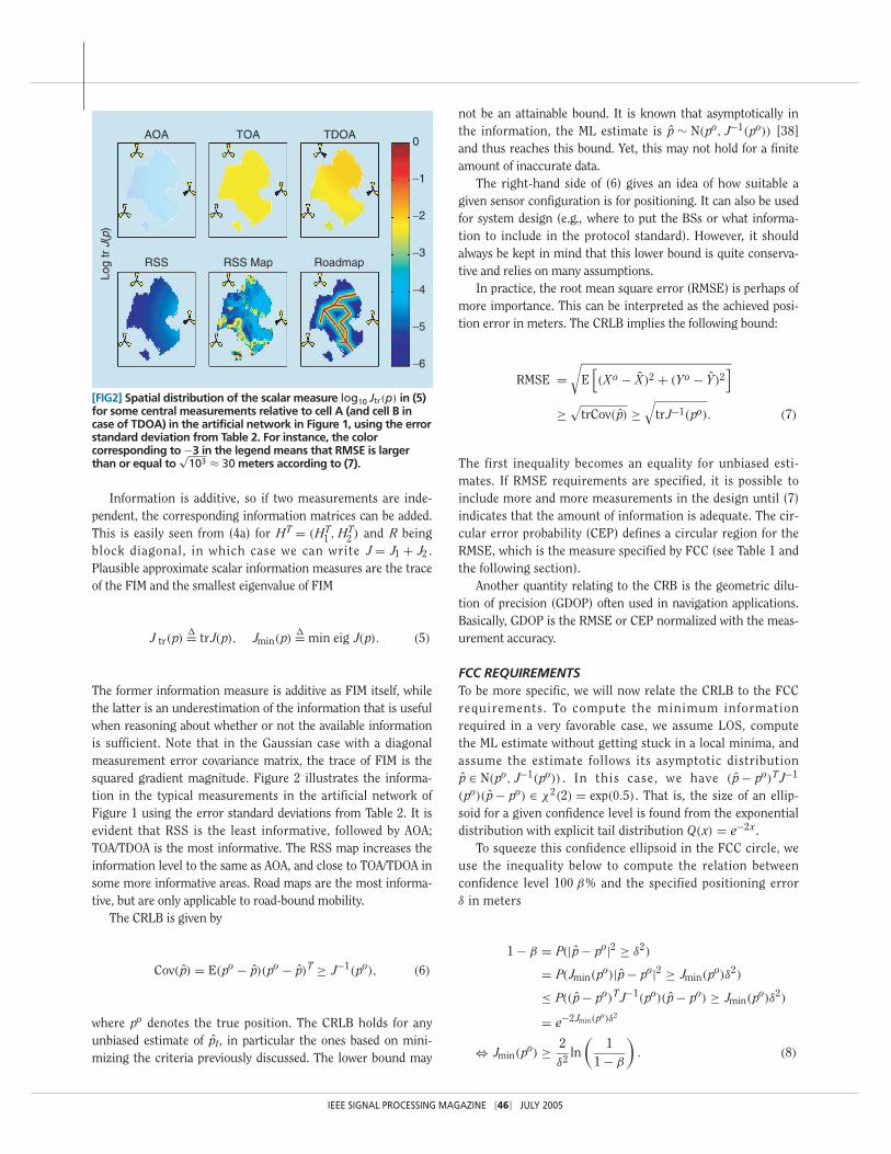
The former information measure is additive as FIM itself, whilethe latter is an underestimation of the information that is usefulwhen reasoning about whether or not the available informationis sufficient. Note that in the Gaussian case with a diagonalmeasurement error covariance matrix, the trace of FIM is thesquared gradient magnitude. Figure 2 illustrates the informa-tion in the typical measurements in the artificial network ofFigure 1 using the error standard deviations from Table 2. It isevident that RSS is the least informative, followed by AOA;TOA/TDOA is the most informative. The RSS map increases theinformation level to the same as AOA, and close to TOA/TDOA insome more informative areas. Road maps are the most informa-tive, but are only applicable to road-bound mobility.

The CRLB is given by

Cov( p) = E(po − p)(po − p)T ≥ J−1(po), (6)

where po denotes the true position. The CRLB holds for anyunbiased estimate of pt, in particular the ones based on mini-mizing the criteria previously discussed. The lower bound may

not be an attainable bound. It is known that asymptotically inthe information, the ML estimate is p ∼ N(po, J−1(po)) [38]and thus reaches this bound. Yet, this may not hold for a finiteamount of inaccurate data.

The right-hand side of (6) gives an idea of how suitable agiven sensor configuration is for positioning. It can also be usedfor system design (e.g., where to put the BSs or what informa-tion to include in the protocol standard). However, it shouldalways be kept in mind that this lower bound is quite conserva-tive and relies on many assumptions.

In practice, the root mean square error (RMSE) is perhaps ofmore importance. This can be interpreted as the achieved posi-tion error in meters. The CRLB implies the following bound:

RMSE =√

E[(Xo − X)2 + (Yo − Y)2

]

≥√

trCov( p) ≥√

tr J−1(po). (7)

The first inequality becomes an equality for unbiased esti-mates. If RMSE requirements are specified, it is possible toinclude more and more measurements in the design until (7)indicates that the amount of information is adequate. The cir-cular error probability (CEP) defines a circular region for theRMSE, which is the measure specified by FCC (see Table 1 andthe following section).

Another quantity relating to the CRB is the geometric dilu-tion of precision (GDOP) often used in navigation applications.Basically, GDOP is the RMSE or CEP normalized with the meas-urement accuracy.

FCC REQUIREMENTSTo be more specific, we will now relate the CRLB to the FCCrequirements. To compute the minimum informationrequired in a very favorable case, we assume LOS, computethe ML estimate without getting stuck in a local minima, andassume the estimate follows its asymptotic distributionp ∈ N(po, J−1(po)) . In this case, we have ( p− po)T J−1

(po)( p− po) ∈ χ2(2) = exp(0.5). That is, the size of an ellip-soid for a given confidence level is found from the exponentialdistribution with explicit tail distribution Q(x) = e−2x.

To squeeze this confidence ellipsoid in the FCC circle, weuse the inequality below to compute the relation betweenconfidence level 100 β% and the specified positioning errorδ in meters

1 − β = P(| p− po|2 ≥ δ2)

= P( Jmin(po)| p− po|2 ≥ Jmin(po)δ2)

≤ P(( p− po)T J−1(po)( p− po) ≥ Jmin(po)δ2)

= e−2 Jmin(po)δ2

⇔ Jmin(po) ≥ 2δ2 ln

(1

1 − β

). (8)

[FIG2] Spatial distribution of the scalar measure log10 Jtr(p) in (5)for some central measurements relative to cell A (and cell B incase of TDOA) in the artificial network in Figure 1, using the errorstandard deviation from Table 2. For instance, the colorcorresponding to −3 in the legend means that RMSE is largerthan or equal to

√103 ≈ 30 meters according to (7).

AOA TOA TDOA

RSS RSS Map Roadmap

−6

−5

−4

−3

−2

−1

0

Log

tr J

(p)


For the FCC requirements in Table 1, we get the minimuminformation [ Jmin(po)] requirements according to Table 6.

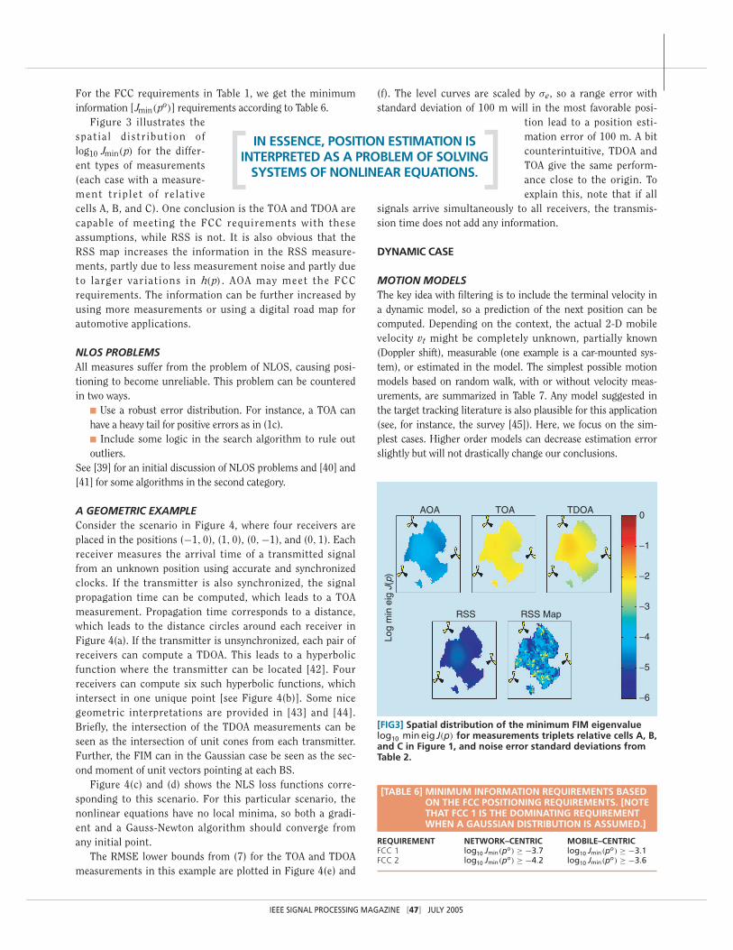
Figure 3 illustrates thespatial distr ibution oflog10 Jmin(p) for the differ-ent types of measurements(each case with a measure-ment tr iplet of relat ivecells A, B, and C). One conclusion is the TOA and TDOA arecapable of meeting the FCC requirements with theseassumptions, while RSS is not. It is also obvious that theRSS map increases the information in the RSS measure-ments, partly due to less measurement noise and partly dueto larger variations in h(p) . AOA may meet the FCCrequirements. The information can be further increased byusing more measurements or using a digital road map forautomotive applications.

NLOS PROBLEMSAll measures suffer from the problem of NLOS, causing posi-tioning to become unreliable. This problem can be counteredin two ways.

■ Use a robust error distribution. For instance, a TOA canhave a heavy tail for positive errors as in (1c).■ Include some logic in the search algorithm to rule outoutliers.

See [39] for an initial discussion of NLOS problems and [40] and[41] for some algorithms in the second category.

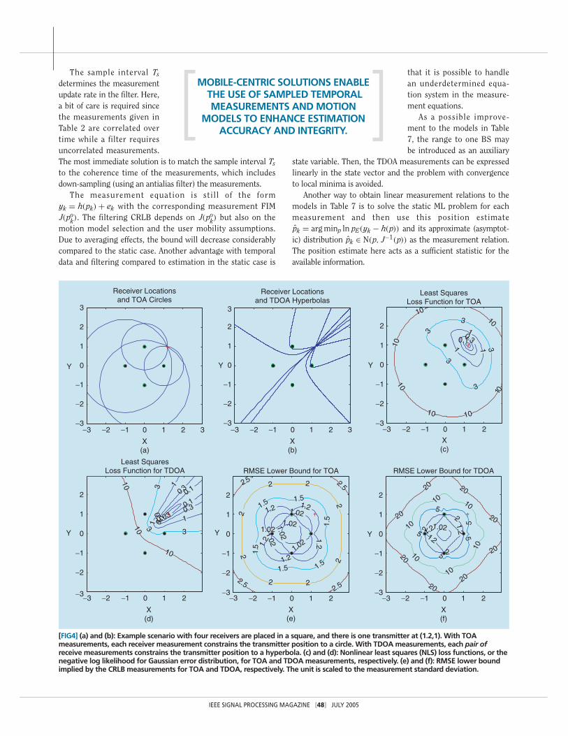
A GEOMETRIC EXAMPLEConsider the scenario in Figure 4, where four receivers areplaced in the positions (−1, 0), (1, 0), (0,−1), and (0, 1). Eachreceiver measures the arrival time of a transmitted signalfrom an unknown position using accurate and synchronizedclocks. If the transmitter is also synchronized, the signalpropagation time can be computed, which leads to a TOAmeasurement. Propagation time corresponds to a distance,which leads to the distance circles around each receiver inFigure 4(a). If the transmitter is unsynchronized, each pair ofreceivers can compute a TDOA. This leads to a hyperbolicfunction where the transmitter can be located [42]. Fourreceivers can compute six such hyperbolic functions, whichintersect in one unique point [see Figure 4(b)]. Some nicegeometric interpretations are provided in [43] and [44].Briefly, the intersection of the TDOA measurements can beseen as the intersection of unit cones from each transmitter.Further, the FIM can in the Gaussian case be seen as the sec-ond moment of unit vectors pointing at each BS.

Figure 4(c) and (d) shows the NLS loss functions corre-sponding to this scenario. For this particular scenario, thenonlinear equations have no local minima, so both a gradi-ent and a Gauss-Newton algorithm should converge fromany initial point.

The RMSE lower bounds from (7) for the TOA and TDOAmeasurements in this example are plotted in Figure 4(e) and

(f). The level curves are scaled by σe, so a range error withstandard deviation of 100 m will in the most favorable posi-

tion lead to a position esti-mation error of 100 m. A bitcounterintuitive, TDOA andTOA give the same perform-ance close to the origin. Toexplain this, note that if all

signals arrive simultaneously to all receivers, the transmis-sion time does not add any information.

DYNAMIC CASE

MOTION MODELSThe key idea with filtering is to include the terminal velocity ina dynamic model, so a prediction of the next position can becomputed. Depending on the context, the actual 2-D mobilevelocity vt might be completely unknown, partially known(Doppler shift), measurable (one example is a car-mounted sys-tem), or estimated in the model. The simplest possible motionmodels based on random walk, with or without velocity meas-urements, are summarized in Table 7. Any model suggested inthe target tracking literature is also plausible for this application(see, for instance, the survey [45]). Here, we focus on the sim-plest cases. Higher order models can decrease estimation errorslightly but will not drastically change our conclusions.

REQUIREMENT NETWORK–CENTRIC MOBILE–CENTRICFCC 1 log10 Jmin(po) ≥ −3.7 log10 Jmin(po) ≥ −3.1FCC 2 log10 Jmin(po) ≥ −4.2 log10 Jmin(po) ≥ −3.6

[TABLE 6] MINIMUM INFORMATION REQUIREMENTS BASEDON THE FCC POSITIONING REQUIREMENTS. [NOTETHAT FCC 1 IS THE DOMINATING REQUIREMENTWHEN A GAUSSIAN DISTRIBUTION IS ASSUMED.]

IN ESSENCE, POSITION ESTIMATION ISINTERPRETED AS A PROBLEM OF SOLVING

SYSTEMS OF NONLINEAR EQUATIONS.

[FIG3] Spatial distribution of the minimum FIM eigenvaluelog10 min eig J(p) for measurements triplets relative cells A, B,and C in Figure 1, and noise error standard deviations fromTable 2.

AOA TOA TDOA

RSS RSS Map

−6

−5

−4

−3

−2

−1

0

Log

min

eig

J(p

)


The sample interval Ts

determines the measurementupdate rate in the filter. Here,a bit of care is required sincethe measurements given inTable 2 are correlated overtime while a filter requiresuncorrelated measurements.The most immediate solution is to match the sample interval Ts

to the coherence time of the measurements, which includesdown-sampling (using an antialias filter) the measurements.

The measurement equation is still of the formyk = h(pk) + ek with the corresponding measurement FIMJ(po

k). The filtering CRLB depends on J(pok) but also on the

motion model selection and the user mobility assumptions.Due to averaging effects, the bound will decrease considerablycompared to the static case. Another advantage with temporaldata and filtering compared to estimation in the static case is

that it is possible to handlean underdetermined equa-tion system in the measure-ment equations.

As a possible improve-ment to the models in Table7, the range to one BS maybe introduced as an auxiliary

state variable. Then, the TDOA measurements can be expressedlinearly in the state vector and the problem with convergenceto local minima is avoided.

Another way to obtain linear measurement relations to themodels in Table 7 is to solve the static ML problem for eachmeasurement and then use this position estimatepk = arg minp ln pE(yk − h(p)) and its approximate (asymptot-ic) distribution pk ∈ N(p, J−1(p)) as the measurement relation.The position estimate here acts as a sufficient statistic for theavailable information.

[FIG4] (a) and (b): Example scenario with four receivers are placed in a square, and there is one transmitter at (1.2,1). With TOAmeasurements, each receiver measurement constrains the transmitter position to a circle. With TDOA measurements, each pair ofreceive measurements constrains the transmitter position to a hyperbola. (c) and (d): Nonlinear least squares (NLS) loss functions, or thenegative log likelihood for Gaussian error distribution, for TOA and TDOA measurements, respectively. (e) and (f): RMSE lower boundimplied by the CRLB measurements for TOA and TDOA, respectively. The unit is scaled to the measurement standard deviation.

−3 −2 −1 0 1 2 3−3

−2

−1

0

1

2

3

X(a)

Y

Receiver Locationsand TOA Circles

−3 −2 −1 0 1 2 3−3

−2

−1

0

1

2

3

X(b)

Y

Receiver Locationsand TDOA Hyperbolas

0.10.31

1 1 3

3

3

3

3

10

10

10

10 10

10

10

X(c)

Y

Least SquaresLoss Function for TOA

−3 −2 −1 0 1 2−3

−2

−1

0

1

2

0.03

0.1

0.1

0.10.3

0.3

0.3

1

1 1

3

3

3

1010

10

X(d)

Y

Least SquaresLoss Function for TDOA

−3 −2 −1 0 1 2−3

−2

−1

0

1

2

1.021.02

1.02

1.02

1.02

1.02

1.2

1.2

1.2

1.21.2

1.5

1.5 1.5

1.5

1.51.5 2

22

2

2

2 2

2

2.5

2.52.5

2.5

X(e)

Y

RMSE Lower Bound for TOA

−3 −2 −1 0 1 2−3

−2

−1

0

1

2

1.021.2

1.21.2

2

2

2

5

5

5

5

5

10

10

10

1010

10

20

20

20

20

20

20

20

20

X(f)

Y

RMSE Lower Bound for TDOA

−3 −2 −1 0 1 2−3

−2

−1

0

1

2

MOBILE-CENTRIC SOLUTIONS ENABLETHE USE OF SAMPLED TEMPORALMEASUREMENTS AND MOTION

MODELS TO ENHANCE ESTIMATIONACCURACY AND INTEGRITY.


POSITION FILTERINGThe simplest approach would be touse adaptive filters similar to thenumerical search schemes in Table4. An adaptive algorithm based onthe steepest descent principle isthe least mean square (LMS) algo-rithm. Similarly, the recursiveleast squares (RLS) algorithm isan adaptive version of a Gauss-Newton search. The tuning param-eter µ or λ controls the amount ofaveraging and reflects our belief inuser mobility rate.

The last two models M3 andM4 in Table 7 require state esti-mation. The natural first attempt is the extended Kalmanfilter (EKF), in which measurement errors are assumedGaussian and the nonlinear measurement equationyk = h(pk) + ek is linearized around the current positionestimate. In case of a highly nonlinear measurement equa-tion h(pk), or non-Gaussian error distribution, the positionestimate using the EKF is far from the CRLB. The comput-er-intensive particle filter (PF) [46], [47] has been proposedfor high-performance positioning [15]. The advantage isthat all currently available information described in the sec-tion on measurements is easily incorporated, includingpower attenuation maps and street maps. Some examplesare provided in [48].

FUNDAMENTAL PERFORMANCE BOUNDSRecently, location performance in the dynamic case interms of the CRLB has been studied in [49]–[51] for theTDOA case. Remember that the CRLB is asymptotic in theinformation, and thus it is a conservative bound also in fil-tering. The CRLB for nonlinear filtering was derived in[52]. In short, they presented a recursion for nonlinearmodels similar to the information filter version of theRiccati equation that computes a lower estimation boundPk. We here present a general result for the random walkmodel M1 and velocity sensor model M2 in Table 7. Withprocess noise covariance matrix Cov(wk) = Qk , both resultin the same recursion

Cov(pk) ≥Pk, (9a)

Pk+1 =((Pk + TsQk)

−1 + J(pok)

)−1. (9b)

In the cases of M3 and M4 with a velocity state in Table 7, defineH = (I, 0). This yields

Cov(pk) ≥HPkHT, (10a)

Pk+1 =((FPkFT + GQkGT)−1 + HT J(po

k)H)−1

. (10b)

These expressions clearly show the compromise between mobility(Q) and information ( J). Later in this article, a few specific casesof special interest will be pointed out.

The position-dependent information matrix J(po) is undermild conditions on the measurement relation h(p) a smooth func-tion and can be considered constant for movements in a smallneighborhood of po. The Riccati recursion will then converge to astationary point. We will in the sequel analyze the first two cases inTable 7 in more detail. For (9b), the stationary value is given by

P =((P + TsQ)−1 + J(po)

)−1, (11)

which has the solution (see “Stationary Riccati Equation forPositioning”)

P = − 12

TsQ + J−1/2(po)

×(

J1/2(po)(TsQ + Ts2

4Q JQ) J1/2(po)

)1/2

J−1/2(po).

(12)

The following procedure thus yields the bound for any wirelesspositioning application.

1) Select measurements from Table 2. 2) Compute the FIM using (4a) and (4b).3) Select a motion model (random walk M1 or velocity sensormodel M2) from Table 7.4) Compute (12).

We can also point out a couple of important special cases.■ For the case with large mobility uncertainty, Q → ∞ and(11) gives Pk = J−1(po), which is the static case. ■ For the case of symmetric movements in more than onedimension, we can assume that Q = qI. The measurementequation can also be assumed to be symmetric in the differentdimensions (it can always be transformed to this form any-way), which means J = Jmin(po)I. This assumption can also

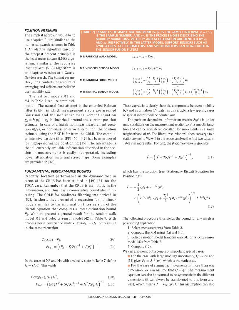
M1: RANDOM WALK MODEL pk+1 = pk + Tswk

M2: VELOCITY SENSOR MODEL pk+1 = pk + Tsvk + Tswk

M3: RANDOM FORCE MODEL(

pk+1

vk+1

)=

(I Ts · I0 I

)︸︷︷︸

F

(pk

vk

)+

(T2

s /2 · ITs · I

)︸︷︷︸

G

wk

M4: INERTIAL SENSOR MODEL(

pk+1

vk+1

)=

(I Ts · I0 I

)(pk

vk

)+

(T2

s /2 · ITs · I

)ak +

(T2

s /2 · ITs · I

)wk

[TABLE 7] EXAMPLES OF SIMPLE MOTION MODELS. [Ts IS THE SAMPLE INTERVAL, k = t/TsIS THE SAMPLE NUMBER, AND wk IS THE PROCESS NOISE DESCRIBING THEMOBILITY VARIATIONS. VELOCITY AND ACCELERATION ARE DENOTED BY vkAND ak, RESPECTIVELY. IN THE LATTER MODEL, SUPPORT SENSORS SUCH ASGYROSCOPES, ACCELEROMETERS, AND SPEEDOMETERS CAN BE INCLUDED INTHE SENSOR FUSION FILTER.]


be seen as a conservative circular bound on the confidenceellipsoid. Then, the asymptotic CRLB according to (12) is

P = qTs

2

(√4

Jmin(po)qTs+ 1 − 1

)I (13a)

≈

1Jmin(po)

I if Jmin(po)qTs4 � 1

√qTs

Jmin(po)I if Jmin(po)qTs

4 � 1.

(13b)

The second case is the normal case, as will be apparentwhen plugging in realistic values. The first case of veryrapid movements and/or very informative measurementscorresponds to the static case.■ For the special case of no movement at all (Q = 0), thesolution is found from (9b) directly (assuming P−1

0 = 0) as

Pk = 1k

J−1(po) = Ts

tJ−1(po). (14)

This case is of interest for MS equipped with a stand-stilldetector (available in some models today for energy-sav-ing purposes).

FCC REQUIREMENTSIt is interesting to establish the relation between the FCCrequirements in Table 1 and the benefits from filtering. A sen-sor configuration that fails the FCC requirements in the staticcase might satisfy the requirements if a sufficient gain from fil-tering is present. Consider the case in the previous section withless informative measurements or very limited movements.After a similar motivation to that seen in the earlier “FCCRequirements” section with the same circular positioning errordistribution assumption, (8) becomes

1√qTs

Jmin(po)

≥ 2δ2 ln

(1

1 − β

), (15a)

Jmin(po) ≥ qTs(δ2

2 ln(1−β)

)2 . (15b)

This constitutes an explicit bound on the information, andalso an implicit upper limit on q to make a certain sensor con-

figuration meet the FCC requirements formulated as the righthand side of (15). Table 8 exemplifies the information neededfor three typical velocity intervals in a random walk modelM1. As seen, considerably less information is needed com-pared to the static case (8). We also note that the assumptionin the Taylor expansion in (13a) is valid for log10( Jmin)

approximately less than −3, even in the car mobility casewhere Var(wk) = q = 302.

In the special case of no movement at all, (8) and (14) com-bine to the information requirement

Jmin(po) ≥ 2kδ2 ln

(1

1 − β

). (16)

The static case is obtained with k = 1, so the standstill case inTable 8 with log10(1) = 0 corresponds to the values in Table 6.

The value of the random walk noise variance q is usuallyconsidered as a design parameter in model-based filtering.The values chosen in Table 8 are merely for illustration pur-poses. In light of how many measurements are required in thestandstill case to reach the other motion states, one mayargue that q should be increased an order of magnitude.However, we leave this as a design issue and conclude that, inany way, the required information is potentially relaxed atleast an order of magnitude by filtering the measurementscompared to a snap-shot approach.

A SIMPLE FILTERING EXAMPLEThe following simplified positioning example illustrates theinterplay of true and modeled motion. The random walk modelM1 in one dimension is given by

pk+1 =pk + wk (17)

yk =pk + ek. (18)

The example can be generalized to independent motions intwo and three dimensions. We assume an A-GPS measurementwith sampling frequency 1 Hz and with Gaussian error withstandard deviation 10 m (σ 2

e = 102). It is further assumed thatall other information can be neglected when A-GPS is avail-able. The true motion corresponds to one of the cases 2–4 inTable 8. Note that without an explicit velocity state, the modelimplies that a walking user may change velocity from 3 m/sforwards to 3 m/s backwards in 1 s.

MOBILITY MOTION STATE √

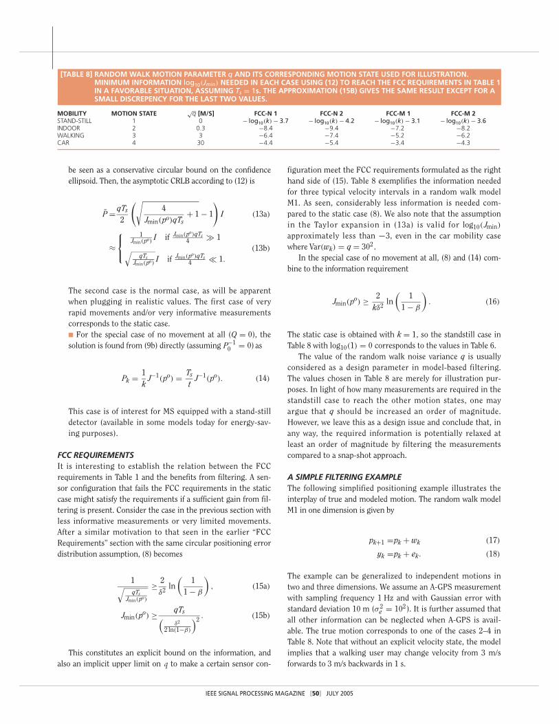
q [M/S] FCC-N 1 FCC-N 2 FCC-M 1 FCC-M 2STAND-STILL 1 0 − log10(k) − 3.7 − log10(k) − 4.2 − log10(k) − 3.1 − log10(k) − 3.6INDOOR 2 0.3 −8.4 −9.4 −7.2 −8.2 WALKING 3 3 −6.4 −7.4 −5.2 −6.2CAR 4 30 −4.4 −5.4 −3.4 −4.3

[TABLE 8] RANDOM WALK MOTION PARAMETER q AND ITS CORRESPONDING MOTION STATE USED FOR ILLUSTRATION.MINIMUM INFORMATION log10(Jmin) NEEDED IN EACH CASE USING (12) TO REACH THE FCC REQUIREMENTS IN TABLE 1IN A FAVORABLE SITUATION, ASSUMING Ts = 1s. THE APPROXIMATION (15B) GIVES THE SAME RESULT EXCEPT FOR ASMALL DISCREPENCY FOR THE LAST TWO VALUES.


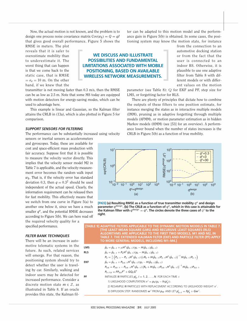
Now, the actual motion is not known, and the problem is todesign one process noise covariance matrix Cov(wk) = Q = qIthat gives good overall performance. Figure 5 shows theRMSE in meters. The plotreveals that it is safer tooverestimate mobility thanto underestimate it. Theworst thing that can happenis that we come back to thestatic case, that is RMSE= σe = 10 m. On the otherhand, if we knew that thetransmitter is not moving faster than 0.3 m/s, then the RMSEcan be as low as 2.5 m. Note that some MS today are equippedwith motion detectors for energy-saving modes, which can beused to advantage here.

This example is linear and Gaussian, so the Kalman filterattains the CRLB in (13a), which is also plotted in Figure 5 forcomparison.

SUPPORT SENSORS FOR FILTERINGThe performance can be substantially increased using velocitysensors or inertial sensors as accelerometersand gyroscopes. Today, these are available forcost and space-efficient mass production withfair accuracy. Suppose first that it is possibleto measure the velocity vector directly. Thisimplies that the velocity sensor model M2 inTable 7 is applicable, and the velocity measure-ment error becomes the random walk inputwk. That is, if the velocity error has standarddeviation 0.3, then q = 0.32 should be usedindependent of the actual speed. Clearly, theinformation requirement can be released thenfor fast mobility. This effectively means thatwe switch from one curve in Figure 5(a) toanother one below it, since we have a muchsmaller qo, and the potential RMSE decreasesaccording to Figure 5(b). We can here read offthe required velocity quality for aspecified performance.

FILTER BANK TECHNIQUESThere will be an increase in auto-motive telematic systems in thefuture. As such, related serviceswill emerge. For that reason, thepositioning system should try todetect whether the user is travel-ing by car. Similarly, walking andindoor users may be detected forincreased performance. Consider adiscrete motion state m ∈ Z , asillustrated in Table 8. If an oracleprovides this state, the Kalman fil-

ter can be adapted to this motion model and the perform-ance gain in Figure 5(b) is obtained. In some cases, the posi-tioning system may know the motion state, for instance

from the connection to anautomotive docking stationor from the fact that theuser is connected to anindoor BS. Otherwise, it isplausible to use one adaptivefilter from Table 8 with dif-ferent models or with differ-ent values on the motion

parameter (see Table 8): Q for EKF and PF, step size forLMS, or forgetting factor for RLS.

There are plenty of principles that dictate how to combinethe outputs of these filters to one position estimate, forinstance merging the states as in interactive multiple models(IMM), pruning as in adaptive forgetting through multiplemodels (AFMM), or motion parameter estimation as in hiddenMarkov models (HMM) (see [53] for an overview). A perform-ance lower bound when the number of states increases is theCRLB in Figure 5(b) as a function of true mobility.

[FIG5] (a) Resulting RMSE as a function of true transmitter mobility qo and designparameter qdesign. (b) The CRLB as a function of qo, which in this case is attainable forthe Kalman filter with qdesign = qo. The circles denote the three cases of qo to theright.

101

100

10−1

10−2 10−1 100 101 102 103 10010−1100

101

102

103

10−2 101 102 103

sqrt

(CR

LB)

qο=qdesign

qο=0.3qο=3qο=30

qdesign

RM

SE

(qde

sign

,qο )

(a) (b)

LMS pk = pk−1 + µHT (pk−1)(yk − H(pk−1)pk−1)

RLS pk = pk−1 + PkHT (pk−1)(yk − H(pk−1)pk−1)

Pk = 1λ

(Pk−1 − Pk−1HT (pk−1)

(λRk + H(pk−1)Pk−1HT (pk−1)

)−1 H(pk−1)Pk−1

)

EKF pk = pk−1 + Pk|k−1HT (pk−1)(yk − H(pk−1)pk−1)

Pk|k = Pk|k−1 − Pk|k−1HT (pk−1)(Rk + H(pk−1)Pk|k−1HT (pk−1)

)−1 H(pk−1)Pk|k−1

Pk+1|k = FPk|kFT + GQkGT

PF INITIALIZE N PARTICLES pi0, i = 1, 2, . . . , N. FOR EACH TIME t:

1) LIKELIHOOD COMPUTATION π i = pE(yk − h(pik)).

2) RESAMPLE N PARTICLES WITH REPLACEMENT ACCORDING TO LIKELIHOOD WEIGHT π i .

3) DIFFUSION STEP: RANDOMIZE w i FROM pW AND LET pik+1 = Fpi

k + Gw i.

[TABLE 9] ADAPTIVE FILTERS APPLICABLE TO THE DYNAMIC MOTION MODELS IN TABLE 7.[THE LEAST MEAN SQUARE (LMS) AND RECURSIVE LEAST SQUARES (RLS)ALGORITHMS ARE APPLICABLE TO THE FIRST TWO MODELS, M1 AND M2, INTABLE 7. THE EXTENDED KALMAN FILTER (EKF) AND PARTICLE FILTER (PF) APPLYTO MORE GENERAL MODELS, INCLUDING M1–M4.]

WE DISCUSS AND ILLUSTRATE POSSIBILITIES AND FUNDAMENTAL

LIMITATIONS ASSOCIATED WITH MOBILEPOSITIONING, BASED ON AVAILABLE

WIRELESS NETWORK MEASUREMENTS.


CONCLUSIONSLocation in wireless networks is of increasing importance forsafety, gaming, and commercial services. There are plenty ofmeasurements available today, ranging from signal arrival timesto maps of received power. We have demonstrated how funda-mental the FIM for each measurement is to assess possible loca-tion performance. As one illustration, the FCC positioningrequirements are transformed to requirements on sufficientinformation. Thereby, it is possible to investigate whether specif-ic sensor configurations would provide acceptable accuracy. Theinformation is additive, so several measurements increase infor-mation. The information concept can also handle less conven-tional measurements, such as digital propagation predictionmaps and road maps. A practical question is whether there is analgorithm that attains the position error lower bound and if it ispossible to implement this algorithm in practice. This, of course,depends from case to case, and we have briefly pointed out algo-rithms of particular interest.

A short road path to implement a positioning system is as follows.

■ 1) Collect the available measurements in Table 2. ■ 2) Compute the static CRB using (3) or using (4a) in the Gaussian case. ■ 3) Compare this to the FCC requirements in Table 1. ■ 4) If these are not satisfied, continue with step 5. Otherwise, evaluate algorithms based on one of the criteria in Table 3 using one of the algorithms in Table 4. If these algorithms do not yield a satisfactory result, continue with step 5.

■ 5) Select a motion model in Table 7. ■ 6) Compare the CRB to the FCC requirements in Table 8.■ 7) If these are satisfied, try to find an algorithm in Table 9that gives satisfactory result. If this fails, try to change thesystem configuration to obtain better measurements, orequip the MS with more sensors.Briefly, the results indicate that the FCC requirement may be

reached using a snapshot localization approach in a most favor-able situation, including LOS and a good estimator. The accura-cy is increased an order of magnitude with filtering andpotentially another order of magnitude with motion sensors.

ACKNOWLEDGMENTSThis work is supported by the competence center InformationSystems for Industrial Control and Supervision (ISIS) and in coop-eration with Ericsson Research.

AUTHORSFredrik Gustafsson is professor in communication systems atthe Department of Electrical Engineering at LinkapingUniversity, Sweden. He received the M.S. degree in electricalengineering in 1988 and the Ph.D. degree in automatic controlin 1992, both from Linkoping University. His research is focusedon statistical signal processing, with applications to automotive,avionics, and communication systems. He is an associate editorof IEEE Transactions of Signal Processing.

Fredrik Gunnarsson is a senior research engineer atEricsson Research and a research associate at LinkopingUniversity, Sweden. He received the M.Sc. degree in 1996 andthe Ph.D. degree in 2000, both in electrical engineering, fromLinkoping University. His research interests include radioresource management and signal processing for wireless com-munications.

REFERENCES[1] J.J. Caffery and G.L. Stuber, “Overview of radiolocation in CDMA cellular sys-tems,” IEEE Commun. Mag., vol. 36, no. 4, pp. 38–45, Apr. 1998.

[2] Y. Zhao, “Standardization of mobile phone positioning for 3G systems,” IEEECommun. Mag., vol. 40, no. 7, pp. 108–116, July 2002.

[3] C. Drane, M. Macnaughtan, and C. Scott. “Positioning GSM telephones,” IEEECommun. Mag., vol. 36, no. 4, pp. 46–54, Apr. 1998.

[4] G. Sun, J. Chen, W. Guo, and K.J.R. Liu, “Signal processing techniques in net-work-aided positioning,” IEEE Signal Processing Mag., vol. 22, no. 4, pp. 12–23, July 2005.

[5] A.H. Sayed, A. Tarighat, and N. Khajehnouri, “Network-based wireless loca-tion,” IEEE Signal Processing Mag., vol. 22, no. 4, pp. 24–40, July 2005.

[6] K. Pahlavan, L. Xinrong, and J.-P. Mäkelä, “Indoor geolocation science andtechnology” IEEE Commun. Mag., vol. 40, no. 2, pp. 112–118, Feb. 2002.

[7] S. Gezici, Z. Tian, G.B. Giannakis, H. Kobayashi, A.F. Molish, H.V. Poor, and Z. Sahinglu, “Localization via ultra-wideband radios,” IEEE Signal ProcessingMag., vol. 22, no. 4, pp. 70–84, July 2005.

[8] N. Patwari, A.O. Hero III, J. Ash, R.L. Moses, S. Kyperountas, and N.S. Correal,“Locating the nodes,” IEEE Signal Processing Mag., vol. 22, no. 4, pp. 54–69, July2005.

[9] D.N. Hatfield, “A report on technical and operational issues impacting the pro-vision of wireless enhanced 911 services,” Federal Communications Commission,Tech. Rep., 2002.

[10] J.J. Caffery, Wireless Location in CDMA Cellular Radio Systems. Norwell, MA:Kluwer, 1999.

[11] Y. Zhao, “Overview of 2G LCS technologies and standards,” in Proc. 3GPP TSGSA2 LCS Workshop, London, UK, Jan. 2001.

[12] K.J. Krizman, T.E. Biedka, and T.S. Rappaport, “Wireless position location:Fundamentals, implementation strategies, and sources of error,” in Proc. IEEEVehicular Technology Conf., June 1997, vol. 2, pp. 919–923.

[13] Y. Okumura, E. Ohmori, T. Kawano, and K. Fukuda, “Field strength and itsvariability in VHF and UHF land-mobile radio service,” Rev. Elec. Commun. Lab.,vol. 16, pp. 9–10, 1968.

[14] M. Hata, “Empirical formula for propagation loss in land mobile radio servic-es,” IEEE Trans. Veh. Technol., vol. 29, no. 3, pp. 317–325 1980.

[15] F. Gustafsson, F. Gunnarsson, N. Bergman, U. Forssell, J. Jansson, R. Karlsson,and P-J. Nordlund, “Particle filters for positioning, navigation and tracking,” IEEETrans. Signal Processing, vol. 50, no. 2, pp. 425–437, Feb. 2002.

[16] R. Karlsson and F. Gustafsson, “Particle filter and Cramér-Rao lower bound forunderwater navigation,” in Proc. IEEE Conf. Acoustics, Speech and SignalProcessing (ICASSP), Hong Kong, China, Apr. 2003, vol. 6, pp. 65–68.

[17] M.C. Vanderveen, A.-J. van der Veen, and A. Paulraj, “Estimation of multipathparameters in wireless communications,” IEEE Trans. Signal Processing, vol. 46,pp. 682–290, Mar. 1998.

[18] C. Botteron, A. Host-Madsen, and M. Fattouche, “Cramér-Rao bound for loca-tion estimation of a mobile in asynchronous DS-CDMA systems,” in Proc. IEEEConf. Acoustics, Speech and Signal Processing, Salt Lake City, UT, May 2001, vol.4, pp. 2221–2224.

[19] E. Strom and F. Malmsten,“A maximum likelihood approach for estimatingDS-CDMA multipath fading channels,” IEEE J. Select. Areas Commun., vol. 18,,no. 1, pp. 132–140, Jan. 2000.

[20] H. Koorapaty, “Cramer-Rao bounds for time of arrival estimation in cellularsystems,” in Proc. IEEE Vehicular Technology Conf., Milan, Italy, May 2004, vol. 5,pp. 2729–2733.

[21] G.G. Raleigh and T. Boros, “Joint space-time parameter estimation for wirelesscommunication channels,” IEEE Trans. Signal Processing, vol. 46, pp. 1333–1343,May 1998.


[22] Y.Qi and H. Kobayashi, “On relation among time delay and signal strengthbased geolocation methods,” in Proc. IEEE Global Telecommunications Conf., SanFrancisco, CA, Dec. 2003, pp. 4079–4083.

[23] A.J. Weiss, “On the accuracy of a cellular location system based on receivedsignal strength measurements,” IEEE Trans. Veh. Technol., vol. 52, no. 6, pp.1508–1518, June 2003.

[24] G. Hendeby and F. Gustafsson, “Fundamental filtering limitations in linearnon-gaussian systems,” in Proc. IFAC World Congress (IFAC'05), Prague, July 2005.

[25] J.O. Smith and J.S. Abel, “Closed-form least-squares source location estima-tion from range-difference measurements,” IEEE Trans. Acoustics, Speech, SignalProcessing, vol. 35, pp. 1661–1669, 1987.

[26] J.E. Dennis, Jr. and B. Schnabel, Numerical Methods for Unconstrained Optimization and Non-linear Equations (Prentice-Hall Series in ComputationalMathematics). Englewood Cliffs, NJ: Prentice-Hall, 1983.

[27] A. Urruela and J. Riba, “Novel closed-form ML position estimator for hyperboliclocation,” in Proc. IEEE Conf. Acoustics, Speech and Signal Processing, Montreal,Canada, May 2004, vol. 2, pp. 149–152.

[28] F. Gustafsson and F. Gunnarsson, “Positioning using time-difference of arrivalmeasurements,” in Proc. IEEE Conf. Acoustics, Speech and Signal Processing(ICASSP), Hong Kong, China, Apr. 2003, vol. 6, pp. 553–556.

[29] S.M. Kay, Fundamentals of Signal Processing—Estimation Theory.Englewood Cliffs, NJ: Prentice Hall, 1993.

[30] C. Botteron, A. Host-Madsen, and M. Fattouche, “Effects of system and envi-ronment parameters on the performance of network-based mobile station positionestimators,” IEEE Trans. Veh. Technol., vol. 53, no. 1, pp. 163–180, Jan. 2004.

[31] C. Botteron, A. Host-Madsen, and M. Fattouche, “Cramer-Rao bounds for theestimation of multipath parameters and mobiles’ positions in asynchronous DS-CDMA systems,” IEEE Trans. Signal Processing, vol. 52, no. 4, pp. 862–875, Jan.2004.

[32] C. Botteron, M. Fattouche, and A. Host-Madsen, “Statistical theory of theeffects of radio location system design parameters on the position performance,” inProc. IEEE Vehicular Technology Conf., Vancouver, Canada, Sept. 2002, pp.1187–1191.

[33] N. Patwari, A.O. Hero III, M. Perkins, N.S. Correal, and R.J. O’Dea, “Relativelocation estimation in wireless sensor networks,” IEEE Trans. Signal Processing,vol. 51, no. 8, pp. 2137–2148, Aug. 2003.

[34] H. Koorapaty, H. Grubeck, and M. Cedervall, “Effect of biased measurementerrors on accuracy of position location methods,” in Proc. IEEE GlobalTelecommunications Conf., Sydney, Australia, Nov. 1998, pp. 1497–1502.

[35] H. Koorapaty, “Barankin bound for position estimation using received signalstrength measurements,” in Proc. IEEE Vehicular Technology Conf., Milan, Italy,May 2004, pp. 2686–2690.

[36] Y. Qi and H. Kobayashi, “On geolocation accuracy with prior information innon-line-of-sight environment,” in Proc. IEEE Vehicular Technology Conf.,Vancouver, Canada, Sept. 2002, pp. 285–288.

[37] Y.Qi and H. Kobayashi, “Cramer-Rao lower bound for geolocation in non-line-of-sight environment,” in Proc. IEEE Conf. Acoustics, Speech and SignalProcessing, Orlando, FL, May 2002, pp. 2473–2476.

[38] E.L. Lehmann, Theory of Point Estimation (Statistical/Probability Series).Belmont, CA: Wadsworth & Brooks/Cole, 1991.

[39] M.P. Wylie and J. Holtzman, “The non-line-of-sight problem in mobile loca-tion estimation,” in Proc. IEEE Int. Conf. Universal Personal Communications,Oct. 1996, pp. 827–831.

[40] J. Riba and A. Urruela, “A non-line-of-sight mitigation technique based onML-detection,” in Proc. IEEE Conf. Acoustics, Speech and Signal Processing,Montreal, Canada, May 2004, vol. 2, pp. 153–156.

[41] J. Zhen and S. Zhang, “Adaptive AR model based robust mobile location esti-mation approach in NLoS environment,” in Proc. IEEE Vehicular TechnologyConf., Milan, Italy, May 2004, pp. 2682–2685.

[42] B.T. Fang, “Simple solutions for a hyperbolic and related position fixes,” IEEETrans. Aerospace and Electronic Systems, vol. 26, no. 5, pp. 748–753, Sept. 1990.

[43] J.S. Abel and J. Chaffee, “Integrating ranging transponders with GPS,” inProc. 1991 ION Nat. Technical Meeting, Phoenix, AZ, 1991, pp. 15–24.

[44] J.S. Abel and J. Chaffee, “The geometry of GPS solutions,” in Proc. 1992Institute of Navigation Nat. Technical Meeting, San Diego, CA, 1992, pp. 425–430.

[45] X.R. Li and V.P. Jilkov, “Survey of maneuvering target tracking. Part I:Dynamic models,” IEEE Trans. Aerosp. Electron. Syst., vol. 39, no. 4, pp.1333–1364, 2003.

[46] N.J. Gordon, D.J. Salmond, and A.F.M. Smith, “A novel approach to nonlin-ear/non-Gaussian Bayesian state estimation,” IEE Proc. Radar Signal Processing,vol. 140, pp. 107–113, 1993.

[47] A. Doucet, N.D. Freitas, and N. Gordon, Eds., Sequential Monte CarloMethods in Practice. New York: Springer-Verlag, 2001.

[48] P-J. Nordlund, F. Gunnarsson, and F. Gustafsson, “Particle filters for position-ing in wireless networks,” in Proc. European Signal Processing Conf. (EUSIPCO),Toulouse, France, Sept. 2002, pp. 311–314.

[49] A. Urruela and J. Riba, “A novel estimator and performance bound for timepropagation and Doppler based radio-location,” in Proc. IEEE Conf. Acoustics,Speech and Signal Processing, Hong Kong, China, Apr. 2003, vol. 5, pp. 253–256.

[50] A. Urruela and J. Riba, “A novel estimator and theoretical limits for in-carradio-location,” in Proc. IEEE Vehicular Technology Conf., Orlando, FL, Oct. 2003,pp. 747–751.

[51] A. Urruela and J. Riba, “Efficient mobile location from time measurementswith unknown variances in dynamic scenarios,” in Proc. IEEE Workshop SignalProcessing Advances in Wireless Communications, Lisbon, Portugal, July 2004,pp. 1522–1526.

[52] N. Bergman, “Posterior Cramér-Rao bounds for sequential estimation,” inSequential Monte Carlo Methods in Practice, A. Doucet, N. de Freitas, and N.Gordon, Eds. New York: Springer-Verlag, 2001, pp. 321–338.

[53] F. Gustafsson, Adaptive Filtering and Change Detection. New York: Wiley, 2000.

APPENDIXSTATIONARY RICCATI EQUATION FOR POSITIONINGEquation (11) can be rewritten first by removing the matrixinversions and then by completing the squares

P−1 = (P + Q)−1 + J(po) (19a)

⇒ PJ(po)P + Q J(po)P = Q (19b)

⇒(

PJ1/2(po) + 12

Q J1/2(po)

)

×(

J1/2(po)P + 12

J1/2(po)Q)

= Q + 14

Q JQ (19c)

⇒(

J1/2(po)PJ1/2(po) + 12

J1/2(po)Q J1/2(po)

)

×(

J1/2(po)PJ1/2(po) + 12

J1/2(po)Q J1/2(po)

)

= J1/2(po)

(Q + 1

4Q JQ

)J1/2(po) (19d)

⇒ P = −12

Q + J−1/2(po)

×(

J1/2(po)(Q + 14

Q JQ) J1/2(po)

)1/2

J−1/2(po).

(19e)

All involved matrices are symmetric, so it follows from(19b) that Q J(po)P is also symmetric, a fact used in the factor-ization (19c). The left and right multiplication with J1/2(po) in(19d) is done to achieve a symmetric solution for P. We havefound one symmetric positive semidefinite solution, and weknow from the general Riccati theory that the solution isunique. Hence, we are done. [SP]

Documents

Mobile Positioning Using Wireless Networksemits.esa.int/...RD24-Mobile-positioning-using-wireless-networks.pdf · tions associated with mobile positioning based on available wireless