M O B I L I T Y

Mobile Network Estimation

Minkyong Kim, Brian NobleMobile Software Systems

University of Michigan

M O B I L I T Y

Adaptive distributed systems

Many systems adapt to changes in network capacitymedia-rich applications: web browsers, video

players, …performance enhancement: caching, prefetching, …distributed systems: query planning, agent

migration, …

All of these systems follow the same general formobserve network traffic at one or both endpointsestimate the latency, bandwidth, loss rate, … react if anything changes in an “interesting” way

All of this depends on estimating network capacity wellturns out to be a difficult problem

M O B I L I T Y

Networks have variable performance

Sources of variation in mobile, wireless networksnodes move, leading to unpredictable topology

changesoften more than one connection alternativephysical layer subject to fading, shadowing, multi-path

Sources of variation in wide-area networksbursty congestion over all time scalesrouting changes between autonomous systems (BGP)

Typically, adaptive systems are evaluated very carefullywith respect to clean, idealized network changesmy own work in Odyssey is guilty as charged

M O B I L I T Y

Goals of a good estimator

Estimate metrics that matter to the systemmany network estimators focus on physical

capacitieslink capacity is like a “speed limit”try driving the speed limit in LA during rush hourinstead: measure available capacities

Provide three characteristicsaccuracy: gives correct estimates in steady stateagility: detect a true shift in capacity rapidlystability: ignore short-lived transient changes

M O B I L I T Y

Current estimators: EWMA filters

Most use exponentially weighted moving average filtersat each time step, incorporate new observation

(Ocurrent)

with old estimate (Eold)using a weighted linear combination:

Ecurrent = (Eold) + (1-)Ocurrent

The term is called the gainlarge gain: biases toward stabilitysmall gain: biases toward agilitygain is set statically

You can’t have your cake and eat it too

M O B I L I T Y

A tale of two estimators

TCP: a stable filter that is too stableestimates round trip time (RTT): segment, ACKstable estimator: gain set to 7/8used to set retransmission timeout (RTO)under rapidly escalating congestion, RTO grows too

slowlyRTO adds “fudge factor” based on variance

Odyssey: an agile filter that is too agileestimates latency and bandwidth for bulk transfersapplications react to change by changing fidelityagile filter: gain set to 1/4 (latency) and 1/8 (bandwidth)transient changes leads to “tail-chasing” adaptationsapplications must add hysteresis to dampen transients

M O B I L I T Y

The rest of this talk

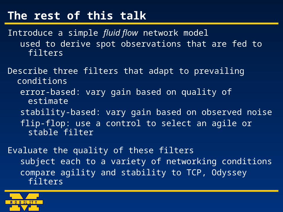
Introduce a simple fluid flow network modelused to derive spot observations that are fed to

filters

Describe three filters that adapt to prevailing conditionserror-based: vary gain based on quality of estimatestability-based: vary gain based on observed noiseflip-flop: use a control to select an agile or stable

filter

Evaluate the quality of these filterssubject each to a variety of networking conditionscompare agility and stability to TCP, Odyssey filters

M O B I L I T Y

A fluid-flow network model

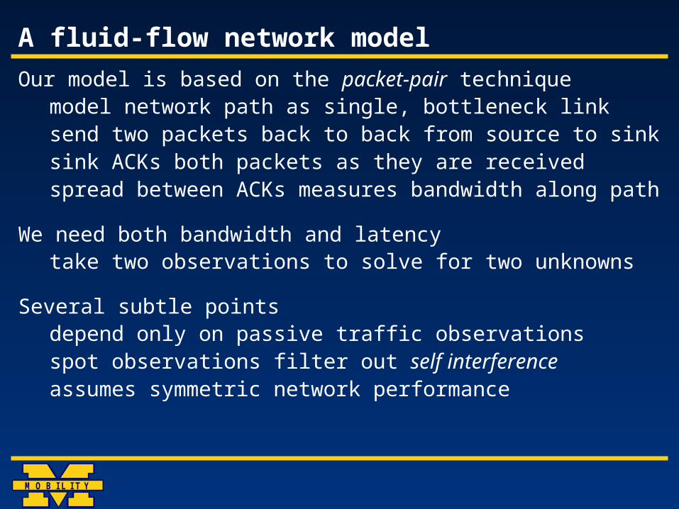
Our model is based on the packet-pair techniquemodel network path as single, bottleneck linksend two packets back to back from source to sinksink ACKs both packets as they are receivedspread between ACKs measures bandwidth along

path

We need both bandwidth and latencytake two observations to solve for two unknowns

Several subtle pointsdepend only on passive traffic observationsspot observations filter out self interferenceassumes symmetric network performance

M O B I L I T Y

The error-based filter

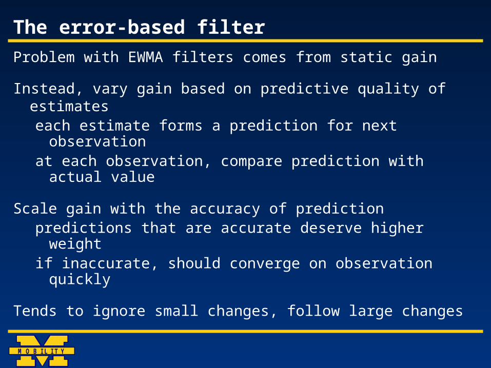
Problem with EWMA filters comes from static gain

Instead, vary gain based on predictive quality of estimateseach estimate forms a prediction for next

observationat each observation, compare prediction with actual

value

Scale gain with the accuracy of predictionpredictions that are accurate deserve higher weightif inaccurate, should converge on observation quickly

Tends to ignore small changes, follow large changes

M O B I L I T Y

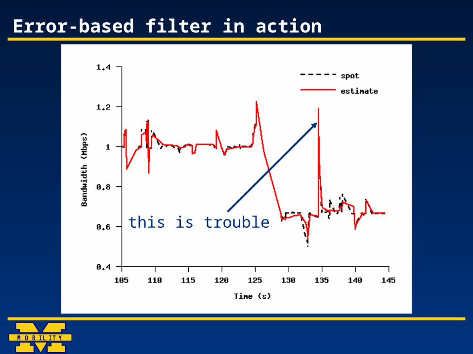
Error-based filter in action

this is trouble

M O B I L I T Y

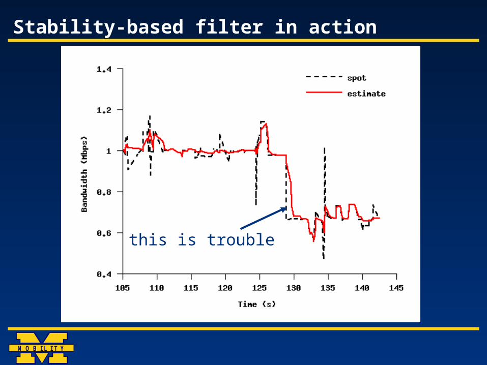
The stability-based filter

The error-based filter will be “pulled” by large transientswill tend towards instability during transient dips

Instead, base gain on stability in recent observationsmoving range: difference between adjacent

observationsnoisy observations lead to larger moving ranges

Scale gain with the magnitude of the moving rangewhen observations are noisy, each deserves less

weightwhen observations are stable, changes more

significant

Tends to ignore large changes, follow small ones

M O B I L I T Y

Stability-based filter in action

this is trouble

M O B I L I T Y

Subtleties in variable-gain filters

The gain in each is based on some source metric

Gain must be in the range [0..1]need some way of scaling the source metricdetermine the maximum {error, instability} recently seenscale current {error, instability} relative to maximum

Transient changes in source metric have drastic effectssmooth observed source metrics by secondary filtersecondary filter has static gain (!)rather than provide tertiary filter, tune empirically

Sometimes, variable-gain filters are neither agile nor stablesource metric places them somewhere in the middle

M O B I L I T Y

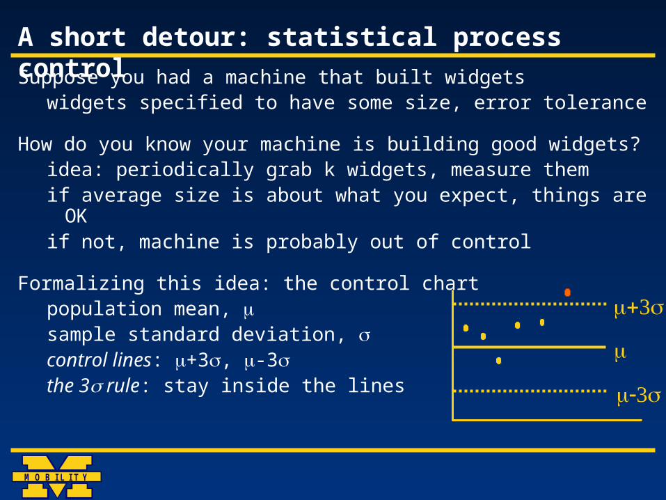
A short detour: statistical process controlSuppose you had a machine that built widgets

widgets specified to have some size, error tolerance

How do you know your machine is building good widgets?idea: periodically grab k widgets, measure themif average size is about what you expect, things are OKif not, machine is probably out of control

Formalizing this idea: the control chartpopulation mean, sample standard deviation, control lines: +3, -3the 3 rule: stay inside the lines

M O B I L I T Y

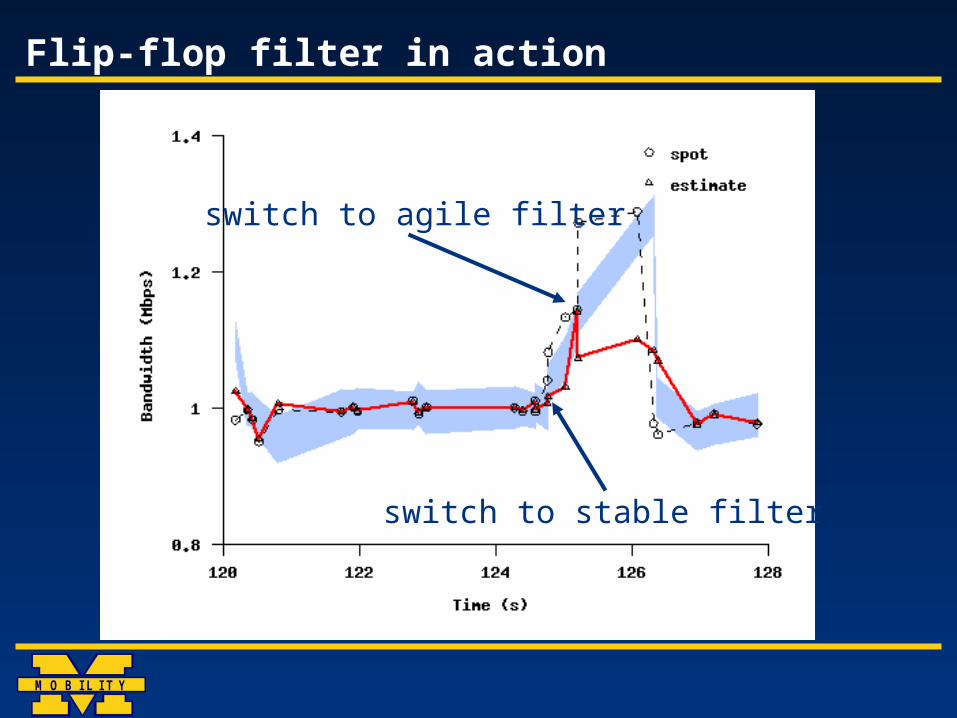
The flip-flop filter

Use a control chart to select for agility, stabilityrun two static-gain EWMA filters in parallelmaintain a control chart for each observationif within control limits, use agile filter ( = 0.1)otherwise, use stable filter ( = 0.9)

Cannot apply simple control chart directly to this problemtrue mean is not known, and it changes over timesample standard deviation is not known

Use approximations (individual x-chart) follows simple smoothed estimate of observations approximated with 2-element moving range

M O B I L I T Y

Flip-flop filter in action

switch to stable filter

switch to agile filter

M O B I L I T Y

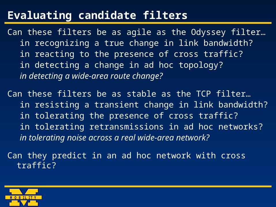
Evaluating candidate filters

Can these filters be as agile as the Odyssey filter…in recognizing a true change in link bandwidth?in reacting to the presence of cross traffic?in detecting a change in ad hoc topology?in detecting a wide-area route change?

Can these filters be as stable as the TCP filter…in resisting a transient change in link bandwidth?in tolerating the presence of cross traffic?in tolerating retransmissions in ad hoc networks?in tolerating noise across a real wide-area network?

Can they predict in an ad hoc network with cross traffic?

M O B I L I T Y

Experimental methodology

All experiments in this talk used ns, a network simulatorthe wide-area set are based on live network traces

Extensions to support variable-link experimentsscript controls base physical performance of a linkcan vary latency, bandwidth over time

Ad hoc networking simulations include Monarch extensionscollision-avoidancelink-level ACK, retransmission

In each experiment, filters converge to same valuethey do not differ in accuracyonly differences in agility, stability

M O B I L I T Y

Link changes

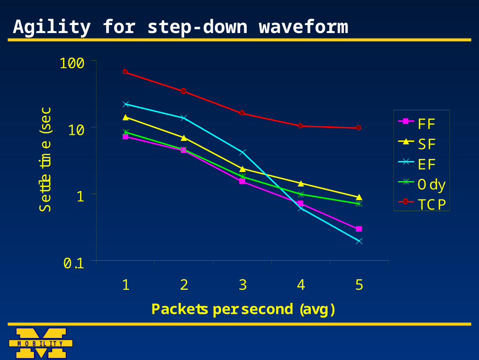
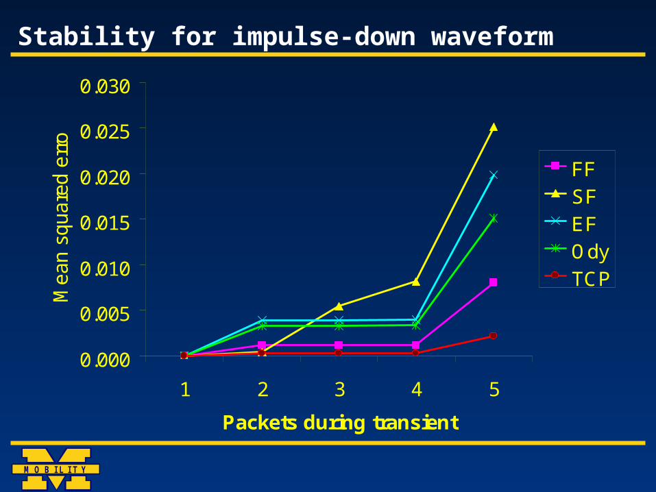
First set of experiments: impulse-response testsconnect client, server with a single ns linkvary link performance with a variant of a square wavepersistent change: decrease from 10Mb/s to 1Mb/stransient change: dip from 10Mb/s to 1Mb/s and back

Vary number of request/response pairs exposed to changepoisson request generator, random response size

Agility: measured by settle timetime to reach an estimate within 10% of nominal

Stability: measured by mean squared errorpenalizes large, short disturbances more than small,

long

M O B I L I T Y

Agility for step-down waveform

0.1

1

10

100

1 2 3 4 5

Packets per second (avg)

Se

ttle

tim

e (

sec)

FFSFEFOdyTCP

M O B I L I T Y

Stability for impulse-down waveform

0.000

0.005

0.010

0.015

0.020

0.025

0.030

1 2 3 4 5

Packets during transient

Mean s

quare

d e

rror

FFSFEFOdyTCP

M O B I L I T Y

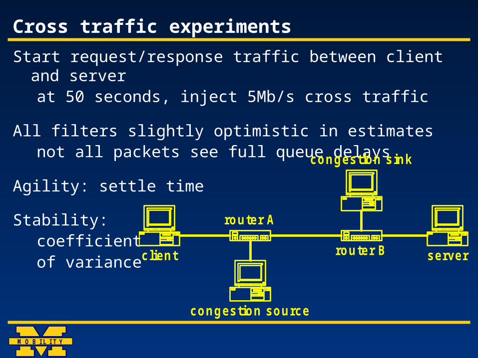
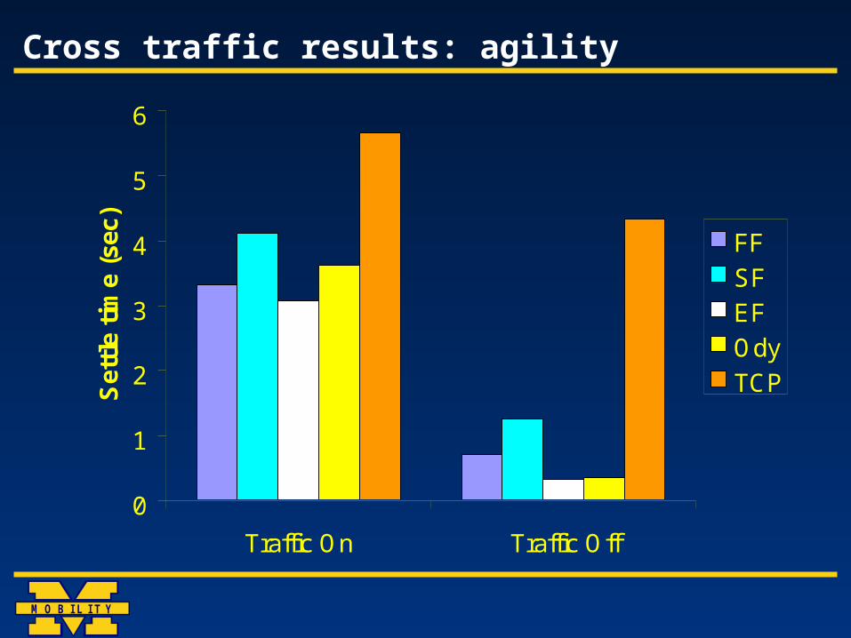
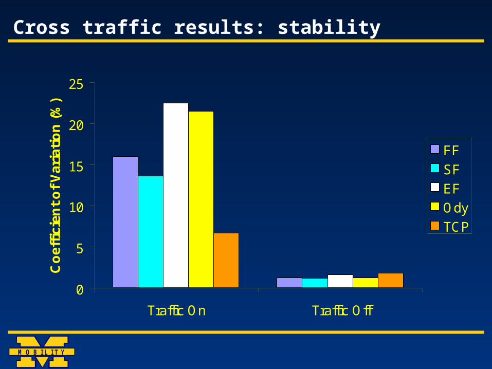
Cross traffic experiments

Start request/response traffic between client and serverat 50 seconds, inject 5Mb/s cross traffic

All filters slightly optimistic in estimatesnot all packets see full queue delays

Agility: settle time

Stability:coefficientof variance

client server

congestion source

congestion sink

router A

router B

M O B I L I T Y

Cross traffic results: agility

0

1

2

3

4

5

6

Traffic On Traffic Off

Set

tle

tim

e (s

ec)

FFSFEFOdyTCP

M O B I L I T Y

Cross traffic results: stability

0

5

10

15

20

25

Traffic On Traffic Off

Co

effi

cien

t o

f V

aria

tio

n (

%)

FF

SF

EF

Ody

TCP

M O B I L I T Y

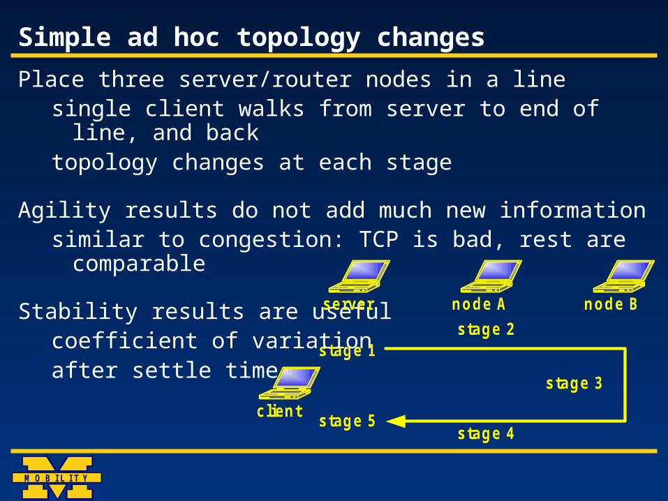
Simple ad hoc topology changes

Place three server/router nodes in a linesingle client walks from server to end of line, and

backtopology changes at each stage

Agility results do not add much new informationsimilar to congestion: TCP is bad, rest are

comparable

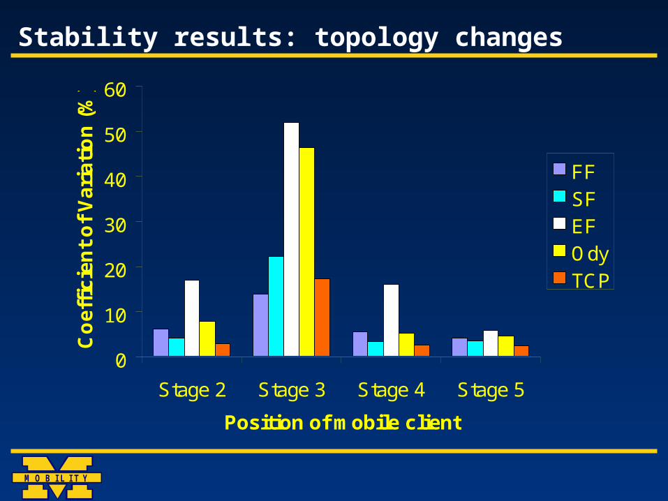
Stability results are usefulcoefficient of variationafter settle time

server node A node B

clientstage 4

stage 5

stage 3

stage 2stage 1

M O B I L I T Y

Stability results: topology changes

0

10

20

30

40

50

60

Stage 2 Stage 3 Stage 4 Stage 5

Position of mobile client

Co

eff

icie

nt

of

Va

ria

tio

n (

%)

FFSFEFOdyTCP

M O B I L I T Y

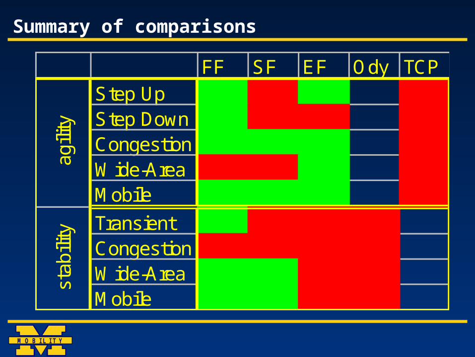
Summary of comparisons

FF SF EF Ody TCPStep UpStep DownCongestionWide-AreaMobile

TransientCongestionWide-AreaMobile

agili

tyst

abili

ty

M O B I L I T Y

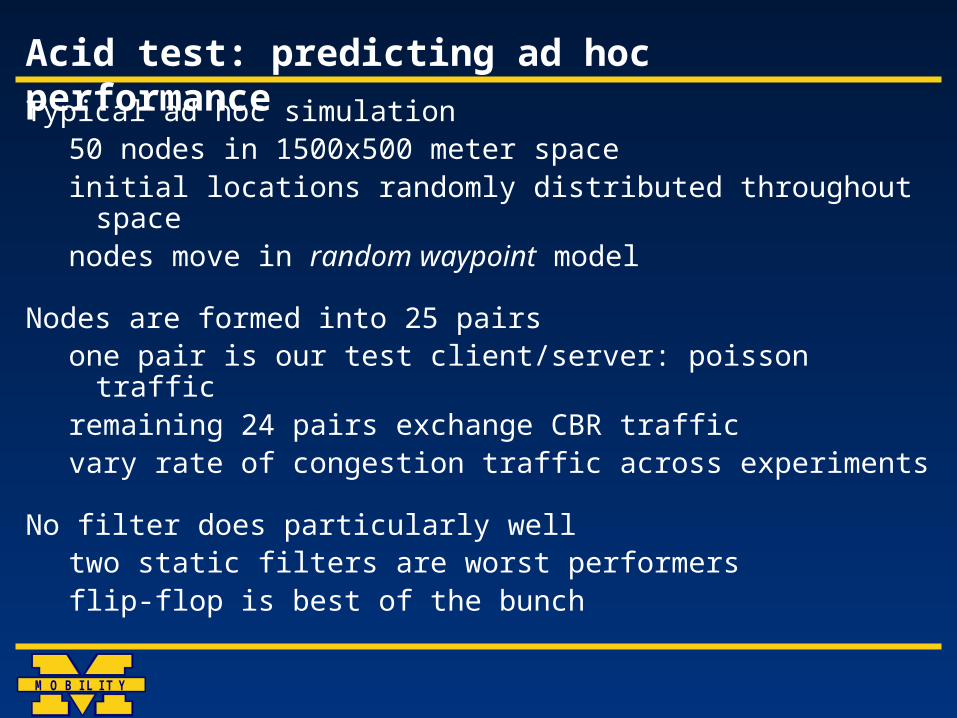
Acid test: predicting ad hoc performanceTypical ad hoc simulation

50 nodes in 1500x500 meter spaceinitial locations randomly distributed throughout

spacenodes move in random waypoint model

Nodes are formed into 25 pairsone pair is our test client/server: poisson trafficremaining 24 pairs exchange CBR trafficvary rate of congestion traffic across experiments

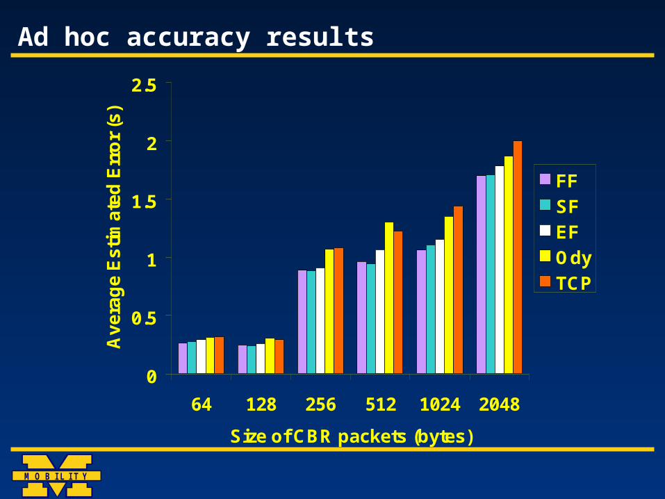
No filter does particularly welltwo static filters are worst performersflip-flop is best of the bunch

M O B I L I T Y

Ad hoc accuracy results

0

0.5

1

1.5

2

2.5

64 128 256 512 1024 2048

Size of CBR packets (bytes)

Av

era

ge

Es

tim

ate

d E

rro

r (s

)

FF

SF

EF

Ody

TCP

M O B I L I T Y

Related WorkS. Keshav: introduced packet-pair, bottleneck bandwidth

fuzzy estimator: similar to error-based estimatoranalysis for rate-allocating servers (not FCFS)

Packet-pair extensions Paxson: receiver-based packet pair: time at both endsLai: receiver-only packet pair: time at receiver

Active probing: Bolot, Downey, Carter & Crovella, …measurement load can be substantial

Lai’s general network model, packet tailgating technique

Balakrishnan’s congestion manager: unified RTT observationscan benefit from our filters for better estimates

M O B I L I T Y

Conclusions

Adaptive systems depend on quality of measurementparticularly hard to estimate network capacity

Standard filtering techniques: agile or stable, but not both

Adaptive filters: tune for prevailing network conditionsagile when possible, stable when necessary

Best alternative: flip-flop filtercomposition of two static-gain EWMA filtersstatistical process control used to select between themcomparable to Odyssey’s agile filter in 4/5 scenarioscomparable to TCP’s stable filter in 3/4 scenariosprovides best predictions in complex ad hoc network

M O B I L I T Y

Questions?

Further details: http://mobility.eecs.umich.edu/

Preprint of the paper is available