Embed Size (px)
Citation preview
ANCOM
Réf : 2012-01-DB-ANCOM
Calculation of the costs of
efficient provision for some
electronic communications
services provided at the
wholesale level in Romania
MOBILE MODEL
DOCUMENTATION
July 2013
PUBLIC VERSION TERA Consultants
39, rue d’Aboukir
75002 PARIS
Tél. + 33 (0) 1 55 04 87 10
Fax. +33 (0) 1 53 40 85 15
www.teraconsultants.fr
S.A.S. au capital de 200 000 €
RCS Paris B 394 948 731
Calculation of the costs of efficient provision for some electronic communications services
provided at the wholesale level in Romania
MOBILE MODULE DOCUMENTATION
Ref : 2012-01 2
Table of contents
List of acronyms ........................................................................................................... 4
0 Context and objectives ......................................................................................... 5
0.1 Disclaimer ..................................................................................................... 5
0.2 Regulatory context ........................................................................................ 5
0.3 Steps of the mobile cost model ..................................................................... 7
1 Networks modeled in the mobile cost model ........................................................10
1.1 Scope of the mobile model ...........................................................................10
1.2 Access network ............................................................................................10
1.3 Core network ...............................................................................................11
1.4 Transmission network ..................................................................................12
2 Subscribers, coverage and service demand ........................................................14
2.1 List of services .............................................................................................14
2.2 Service Demand description ........................................................................15
2.2.1 Mobile subscribers base .......................................................................16
2.2.2 Annual demand (traffic) ........................................................................17
2.3 Coverage requirements ...............................................................................18
2.4 Dimensioning Traffic during the busy hour ...................................................19
2.4.1 Inclusion of non-commercial traffic .......................................................19
2.4.2 Traffic during the Busy Hour .................................................................20
3 Network dimensioning .........................................................................................23
3.1 Routing matrix ..............................................................................................23
3.2 Radio Access Network dimensioning (Sheets 4.2 for 2G and 4.3 for 3G) .....24
3.2.1 Main inputs ...........................................................................................25
3.2.1.1 Spectrum and technology................................................................25
3.2.1.2 Geotypes ........................................................................................25
3.2.1.3 Main engineering inputs ..................................................................27
3.2.2 Radio access network dimensioning – Coverage .................................31
3.2.2.1 Dimensioning rules..........................................................................31
3.2.2.2 Results for the generic operator ......................................................32
3.2.3 Radio access network dimensioning – Capacity ...................................33
3.2.3.1 Traffic capacity calculation ..............................................................33
3.2.3.2 Utilisation factors .............................................................................34
3.2.3.3 Erlang B table .................................................................................34
3.2.3.4 Frequency reuse patterns ...............................................................34
3.2.3.5 2G traffic network dimensioning ......................................................35
3.2.3.6 3G traffic network dimensioning ......................................................36
3.2.3.7 Results for the generic operator ......................................................39
3.3 BSC and RNC equipment dimensioning (Sheets #4.2 for BSC and #4.3 for
RNC) 42
3.3.1 BSC dimensioning rules .......................................................................42
3.3.2 RNC dimensioning rules .......................................................................42
Calculation of the costs of efficient provision for some electronic communications services
provided at the wholesale level in Romania
MOBILE MODULE DOCUMENTATION
Ref : 2012-01 3
3.4 Core network dimensioning (Sheet #4.4) .....................................................43
3.4.1 MGW and MSC-S dimensioning rules ..................................................43
3.4.2 SGSN/GGSN dimensioning rules .........................................................44
3.4.3 SMSC/MMSC dimensioning rules ........................................................45
3.4.4 HLR/VLR dimensioning rules ...............................................................45
3.4.5 IN dimensioning rules ...........................................................................46
3.5 Transmission network dimensioning (Sheet #4.5) ........................................47
4 Unit costs and OPEX ...........................................................................................52
4.1 Network element unit CAPEX (Sheet #5) .....................................................52
4.2 Network element OPEX ...............................................................................52
4.3 Total Network annual cost ............................................................................53
5 Additional costs (non-network costs) ...................................................................54
5.1 Interconnection specific costs ......................................................................54
5.2 Licence costs ...............................................................................................54
5.3 Subscriber access........................................................................................55
5.4 Business overheads .....................................................................................55
5.5 Conversion rules for non-network costs .......................................................56
6 Depreciation ........................................................................................................57
7 Cost allocation .....................................................................................................59
7.1 LRAIC+ cost allocation approach .................................................................59
7.1.1 Total annual costs allocation ................................................................59
7.1.2 Additional costs allocation ....................................................................60
7.2 Pure LRIC cost allocation approach .............................................................60
8 Main results .........................................................................................................62
9 Model Calibration .................................................................................................62
10 List of illustrations and tables ...............................................................................64
11 Appendix .............................................................................................................66
11.1 Annual demand in Romania .........................................................................66
11.1.1 Benchmark of monthly outgoing traffic per subscriber ..........................66
11.1.2 Forecast of monthly ADPU in UK and Romania ...................................67
11.1.3 3G services monthly traffic evolution in Romania .................................67
11.2 Annual traffic to BH traffic conversion factors ...............................................68
11.3 Conversion rules for non-network costs .......................................................69
11.4 Generic operator routing matrix....................................................................72
11.5 Summary of equipment unit CAPEX (MEA) .................................................73
11.6 Description of Pure_LRIC Macro ..................................................................73
Calculation of the costs of efficient provision for some electronic communications services
provided at the wholesale level in Romania
MOBILE MODULE DOCUMENTATION
Ref : 2012-01 4
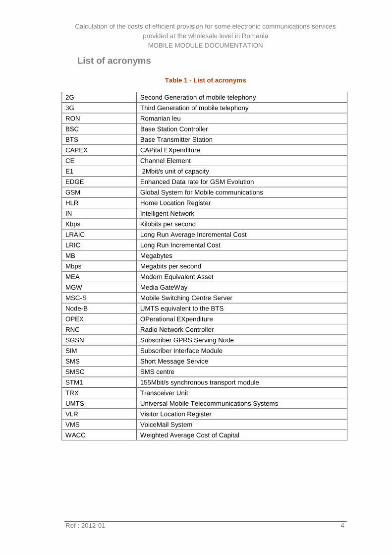
List of acronyms
Table 1 - List of acronyms
2G Second Generation of mobile telephony
3G Third Generation of mobile telephony
RON Romanian leu
BSC Base Station Controller
BTS Base Transmitter Station
CAPEX CAPital EXpenditure
CE Channel Element
E1 2Mbit/s unit of capacity
EDGE Enhanced Data rate for GSM Evolution
GSM Global System for Mobile communications
HLR Home Location Register
IN Intelligent Network
Kbps Kilobits per second
LRAIC Long Run Average Incremental Cost
LRIC Long Run Incremental Cost
MB Megabytes
Mbps Megabits per second
MEA Modern Equivalent Asset
MGW Media GateWay
MSC-S Mobile Switching Centre Server
Node-B UMTS equivalent to the BTS
OPEX OPerational EXpenditure
RNC Radio Network Controller
SGSN Subscriber GPRS Serving Node
SIM Subscriber Interface Module
SMS Short Message Service
SMSC SMS centre
STM1 155Mbit/s synchronous transport module
TRX Transceiver Unit
UMTS Universal Mobile Telecommunications Systems
VLR Visitor Location Register
VMS VoiceMail System
WACC Weighted Average Cost of Capital
Calculation of the costs of efficient provision for some electronic communications services
provided at the wholesale level in Romania
MOBILE MODULE DOCUMENTATION
Ref : 2012-01 5
0 Context and objectives
0.1 Disclaimer
This report contains the methodology of the Mobile Model module provided to ANCOM
to calculate the cost of a mobile operator. It is based on the materials supplied to us by
ANCOM and Romanian operators as well as data available from other public models.
We have used reasonable and proper care to cross-check and investigate the material
supplied so that the methodology follows as much as possible Romanian specificities.
Consequently conclusions drawn in this report may not be suitable in other context.
0.2 Regulatory context
Taking into account the European Commission Recommendation mentioned under
Article 15 of the Directive 2002/21/CE, ANCOM reviewed beginning 2012 the different
relevant markets in order to identify operators with a significant market power.
Pursuant to these decisions, ANCOM with the assistance of TERA Consultants
published the Conceptual Framework in which it is specified how costs should be
measured to provide electronic communication services.
ANCOM with the assistance of TERA Consultants has therefore built up a draft bottom-
up mobile network model in which the following major characteristics are implemented
in accordance with the conceptual framework:
Network dimensioning is based on a scorched node approach;
Annuities evolved according to a yearly approach;
Incremental approach to service costing;
Two scenarios have been considered:
1. Four specific operators scenario based on: Vodafone’s, Orange’s,
Cosmote’s and RCS&RDS’ current mobile networks.
2. Generic operator scenario where the modeled operator is different from any
existing operator and reflects a reasonably efficient Romanian mobile
operator with:
a. a target market share of 20%-25%
b. a spectrum assignment of 10 Mhz in both 900 Mhz and 1800 Mhz
bandwidths, and 15 Mhz in 2100 Mhz bandwidth.
To develop these models, ANCOM held, with the assistance of TERA Consultants,
several meetings with the different mobile operators in order to:
Calculation of the costs of efficient provision for some electronic communications services
provided at the wholesale level in Romania
MOBILE MODULE DOCUMENTATION
Ref : 2012-01 6
Explain extensive data requests that have been circulated to operators
regarding costs, services, network deployments, etc. ; and
Get a deep understanding of their mobile network.
Following the provision of operators’ answers, ANCOM and TERA Consultants first
crosschecked the consistency of the information provided with:
ANCOM statistics data base;
Benchmarks; and
TERA’s experience.
When some data was not provided by the operators, or when data submitted was
inconsistent with other data, the model uses as much as possible data available from
other regulators.
Based on this analysis, ANCOM and TERA Consultants built up a “service” module that
determines the volume of traffic of the different services to be handled by the operator
considered.
This Service Demand Module model has as a starting point real historic demand levels
for the period 2006 – 2010 (or 2011 when available), and includes forecasts for the
period 2012 – 2020. The results of the service module are described below.
Other data provided by operators form key inputs of mobile model that enables to
determine services costs.
The goal of the following document is to describe the assumptions, parameters,
procedures and methodologies used in the model. Due to the confidentiality of some
data, not all inputs and parameters can be shown. The document is structured as
follows:
Description of the different networks modeled in the mobile model (see
section 1);
Description of the data used for the traffic and the number of users for
each service (see section 0);
Description of the different engineering rules used by the different
equipment (see section 3);
Description of the asset prices and the OPEX (see section 4);
Description of the additional non-network costs (see section 5);
Description of the different depreciation methods (see section 6);
Description of the different allocations made in the model (see section
7);
Description of some main results (see section 8).
Calculation of the costs of efficient provision for some electronic communications services
provided at the wholesale level in Romania
MOBILE MODULE DOCUMENTATION
Ref : 2012-01 7
0.3 Steps of the mobile cost model
The purpose of the model is to:
dimension the modeled mobile network based on current and future service
demand;
to calculate the cost of this dimensioned network with relevant depreciation
method;
to allocate the cost between the different services (and especially the wholesale
voice call termination);
and finally to calculate the long run incremental cost of each service.
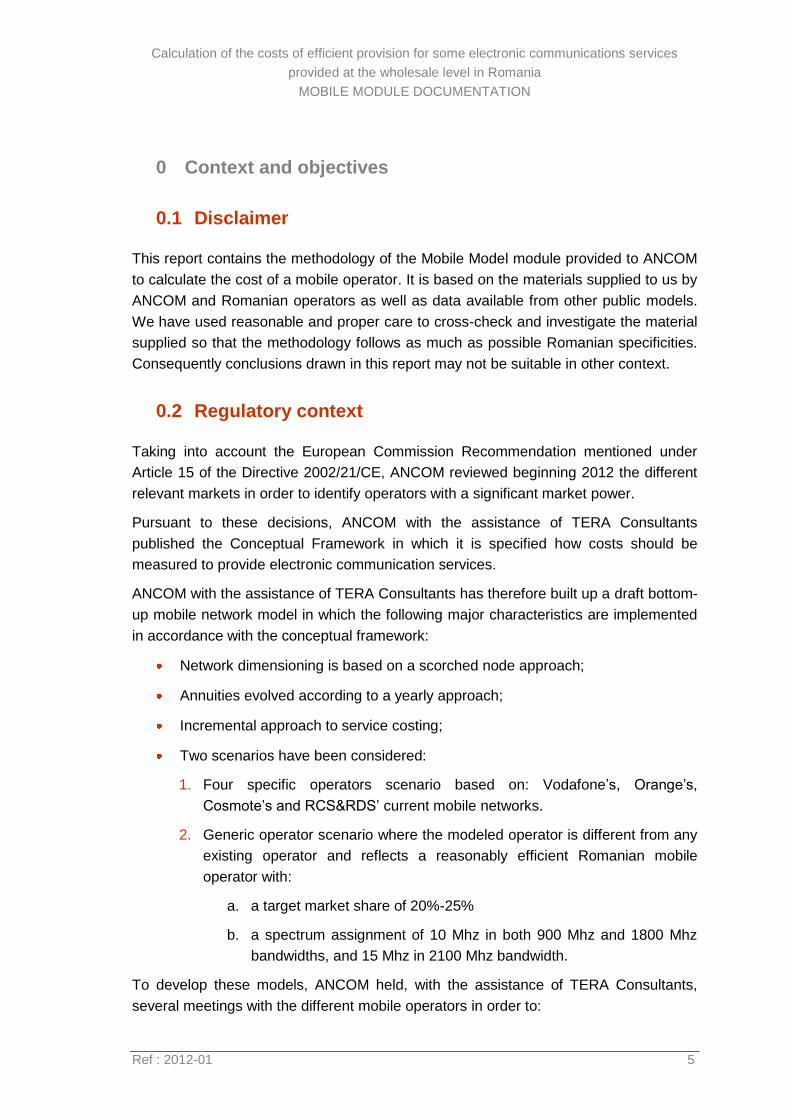
The general model approach is summarized in the figure below.
Figure 1 - Overview of the mobile model
Source: TERA Consultants
1. Raw data
Operators responses
2. Treated data
TERA analysis
5. Unit CAPEX
OPEX
1.1 Vodafone 2.1 Vodafone
1.2 Orange 2.2 Orange
4.2 2G Access
Design
0. Control Panel & Summary of ResultsService Module1.5 Ancom pop data
1.3 Cosmote 2.3 Cosmote
3.0 Selected
operator
8.3 Pure LRIC Cost
w/ eco deprc.8.1 Economic Costs
8.2 Termination
cost calc.
7.1 Service costing
(network)7.2 Other costs 7.3 Pure LRIC
4.0 Design parameters6. Network costs
4.3 3G Access
Design4.4 Core Design
4.5 Transmission
Design
2.5 Generic
1.4 RCS&RDS4.1 Traffic Routing factor
2.4 RCS&RDS
Calculation of the costs of efficient provision for some electronic communications services
provided at the wholesale level in Romania
MOBILE MODULE DOCUMENTATION
Ref : 2012-01 8
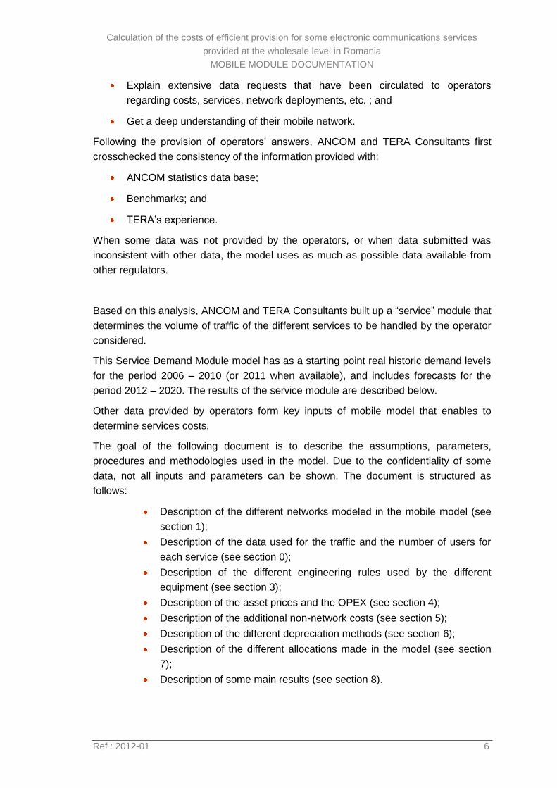
The different steps of the mobile module are described in the figure below:
Figure 2 - Outline of the mobile network module and the interaction with the service
demand module
Source: TERA Consultants
Part 1 – Network topology: The location of nodes along with the required type
of equipment (RNC, MSC, servers) will be determined ;
Part 2 – Future demand: For each mobile operator and for each service
required, forecasts about the future evolution of traffic will be defined. For the
generic operator, assumptions will be made corresponding to the values for the
generic operator market share;
Part 3 – Dimensioning the network: This step consists of determining the
type and number of assets based on engineering rules that are required at each
level of the network to fulfill the demand (the traffic). One important part of this
step consists of creating the routing table. For each service, the equipment and
links that the service uses are determined;
Part 4 – Network costing: This part consists in calculating the corresponding
total cost for the modeled network:
o Populating the model with the prices of the assets used;
o Multiplying the number of assets by the price of these assets;
o Depreciating the CAPEX to annualize the investment cost into annual
charges;
o OPEX are added to the investments’ annual charges.
Calculation of the costs of efficient provision for some electronic communications services
provided at the wholesale level in Romania
MOBILE MODULE DOCUMENTATION
Ref : 2012-01 9
Part 5 – Cost allocation: Costs are allocated to the different services
according to the selected allocation key (routing factors’ table, required
capacity, etc);
Part 6 – Service costs: The cost model calculated for each service its cost per
unit.
Calculation of the costs of efficient provision for some electronic communications services
provided at the wholesale level in Romania
MOBILE MODULE DOCUMENTATION
Ref : 2012-01 10
1 Networks modeled in the mobile cost model
1.1 Scope of the mobile model
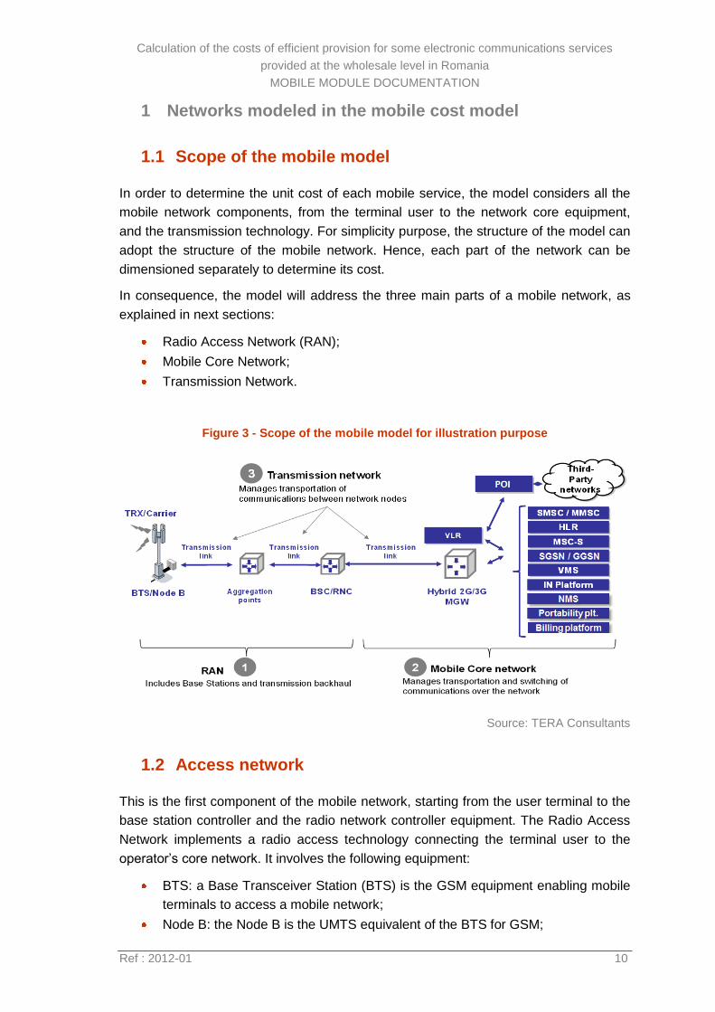
In order to determine the unit cost of each mobile service, the model considers all the
mobile network components, from the terminal user to the network core equipment,
and the transmission technology. For simplicity purpose, the structure of the model can
adopt the structure of the mobile network. Hence, each part of the network can be
dimensioned separately to determine its cost.
In consequence, the model will address the three main parts of a mobile network, as
explained in next sections:
Radio Access Network (RAN);
Mobile Core Network;
Transmission Network.
Figure 3 - Scope of the mobile model for illustration purpose
Source: TERA Consultants
1.2 Access network
This is the first component of the mobile network, starting from the user terminal to the
base station controller and the radio network controller equipment. The Radio Access
Network implements a radio access technology connecting the terminal user to the
operator’s core network. It involves the following equipment:
BTS: a Base Transceiver Station (BTS) is the GSM equipment enabling mobile
terminals to access a mobile network;
Node B: the Node B is the UMTS equivalent of the BTS for GSM;
Calculation of the costs of efficient provision for some electronic communications services
provided at the wholesale level in Romania
MOBILE MODULE DOCUMENTATION
Ref : 2012-01 11
2G/3G IBS: an In Building Solution (IBS) is a low power mobile network cell,
covering a limited area (hotel, train station, shopping center, etc…);
TRX: a Transceiver (TRX) is an equipment combining both a transmitter (TX)
and a receiver (RX). Such equipment enables sending and receiving wireless
signals;
3G Transceiver: A 3G Transceiver is a TRX specific to 3G networks;
Aggregators: is a network equipment which aggregates traffic coming from
different base stations. It represents an intermediary step between the base
stations and the BSC/RNC equiplent;
BSC: the Base Station Controller (BSC) handles traffic and signaling between
mobile devices and a GSM network;
RNC: The Radio Network Controller (RNC) is the UMTS equivalent of the BSC
for GSM. It controls the Node B connected to it and carries out radio resource
management and some of the mobility management functions;
Consistent with realities in the Romanian market, the model uses four access
technologies and spectrum bands:
GSM in 900 MHz band using 2 x 200 KHz channels
GSM in 1800 MHz banduisng 2 x 200 KHz channels
UMTS in 2100 MHz band using 2 x 5 MHz channels
UMTS in 900 MHz band using 2 x 5 MHz channels
1.3 Core network
This is the central part of the operator’s telecommunication network. It provides various
services to customers connected through the access network. The model includes a
forward-looking network structure implementation assuming hybrid 2G/3G MGWs and
MSC-S as described in below sections. According to data gathered from operators and
TERA Consultants expertise, the core network described in the model involves the
following equipment:
MGW (hybrid 2G/3G): the Media GateWay translates media streams between
different telecommunication networks (2G, 3G, IP, etc…);
MSC-S (hardware and software): the Mobile Switching Centre Server (MSC-S)
is an equipment controlling network switching subsystem elements. It carries
out switching and mobility management functions;
SGSN: the Serving GPRS Support Node (SGSN) is the gateway between the
RNC and the core network in a GPRS/EDGE/UMTS network;
GGSN: the Gateway GPRS Support Node (GGSN) is the gateway between the
core network and IP networks to the internet;
SMSC: the SMS Centre (SMSC) is the network equipment switching SMS
traffic;
Calculation of the costs of efficient provision for some electronic communications services
provided at the wholesale level in Romania
MOBILE MODULE DOCUMENTATION
Ref : 2012-01 12
MMSC: the Multimedia Message Service Center (MMSC) is the network
equipment switching MMS traffic;
HLR: the Home Location Register (HLR) is a database storing all the
subscribers’ data;
VMS: the Voice Message Server offers a service whereby calls received when
the mobile is in use, switched off or out of coverage, can be diverted to an
answering service which can be personalized by the user;
VLR: the Visitor Location Register (VLR) is a database attached to a BSS (Base
Station Subsystem, which includes base stations, backhaul and BSC/RNC),
storing data of the subscribers in its area;
IN: the Intelligent Network (IN) is a standard network architecture enabling
operators to provide value-added services on mobile phones;
NMS: the Network Monitoring System (NMS) monitors network equipment and
notifies administrators and/or operators in case of failures;
Portability Platform: the Portability Platform allows subscribers to switch
between mobile operators, while keeping the same phone number;
Billing Platform: the Billing Platform gathers subscribers’ usage and generates
their bills.
1.4 Transmission network
This part of the network ensures the transmission of calls and data between the
different network equipment (nodes), either in the access network or in the core
network. Transmission network is split into two sub-networks:
Backhaul: the part of transmission network ensuring transport of calls and data
through access network nodes
Backbone: the part of transmission network ensuring transport of calls and data
through core network nodes
Different technologies are used in order to link between network nodes:
Wireless: Microwave solutions are implemented in the model through
equipment allowing the transportation of information with varying bandwidth
according to the spectrum of operation:
o 7 Mhz link: allowing to carry the equivalent of 16 E1
o 14 Mhz link: allowing to carry the equivalent of 32 E1
o 28 Mhz link: allowing to carry the equivalent of 64 E1
Wireline: This can be either of the following solutions:
o Own Fiber
o Leased lines

Calculation of the costs of efficient provision for some electronic communications services
provided at the wholesale level in Romania
MOBILE MODULE DOCUMENTATION
Ref : 2012-01 13
o Dark Fiber1
1 For simplicity reason, the model focuses only on leased lines and own fiber
Calculation of the costs of efficient provision for some electronic communications services
provided at the wholesale level in Romania
MOBILE MODULE DOCUMENTATION
Ref : 2012-01 14
2 Subscribers, coverage and service demand
The first step to calculate the LRIC unit costs (whether it is LRAIC+ or “pure LRIC”2) is
to estimate the amount of capacity required to handle the subscribers, coverage
requirements and traffic demand in Romania during the study period.
Specifically, the model forecasts the following items for the period 2006-2020:
Total mobile subscribers and operator specific mobile subscribers (which
depends on the market share);
Territory coverage requirements per geotype;
Annual demand (with traffic breakdown) for each operator;
Traffic during the busy hour for each operator.
Mobile subscribers and annual traffic demand information are calculated in the “Service
Module” which calculates and forecasts them, relying on data received from the
operators, ANCOM, international studies and publicly available databases (such as
public models from other countries). Other items are calculated in the “Mobile Module”
model and the details of each item are provided in the subsections below.
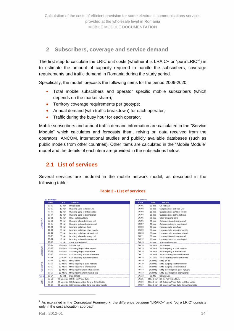
2.1 List of services
Several services are modeled in the mobile network model, as described in the
following table:
Table 2 - List of services
2 As explained in the Conceptual Framework, the difference between “LRAIC+” and “pure LRIC” consists
only in the cost allocation approach
2G Services 3G Services
Code Unit Service Code Unit Service
2G 01 2G min On Net calls 3G 01 3G min On Net calls
2G 02 2G min Outgoing Calls to Fixed Line 3G 02 3G min Outgoing Calls to Fixed Line
2G 03 2G min Outgoing Calls to Other Mobile 3G 03 3G min Outgoing Calls to Other Mobile
2G 04 2G min Outgoing Calls to International 3G 04 3G min Outgoing Calls to International
2G 05 2G min Other Outgoing Calls 3G 05 3G min Other Outgoing Calls
2G 06 2G min Outgoing inbound roaming call 3G 06 3G min Outgoing inbound roaming call
2G 07 2G min Outgoing outbound roaming call 3G 07 3G min Outgoing outbound roaming call
2G 08 2G min Incoming calls from fixed 3G 08 3G min Incoming calls from fixed
2G 09 2G min Incoming calls from other mobile 3G 09 3G min Incoming calls from other mobile
2G 10 2G min Incoming calls from international 3G 10 3G min Incoming calls from international
2G 11 2G min Incoming inbound roaming call 3G 11 3G min Incoming inbound roaming call
2G 12 2G min incoming outbound roaming call 3G 12 3G min incoming outbound roaming call
2G 13 2G min Voice Mail Retrieval 3G 13 3G min Voice Mail Retrieval
2G 14 2G SMS SMS on net 3G 14 3G SMS SMS on net
2G 15 2G SMS SMS outgoing to other network 3G 15 3G SMS SMS outgoing to other network
2G 16 2G SMS SMS outgoing to international 3G 16 3G SMS SMS outgoing to international
2G 17 2G SMS SMS incoming from other network 3G 17 3G SMS SMS incoming from other network
2G 18 2G SMS SMS incoming from international 3G 18 3G SMS SMS incoming from international
2G 19 2G MMS MMS on net 3G 19 3G MMS MMS on net
2G 20 2G MMS MMS outgoing to other network 3G 20 3G MMS MMS outgoing to other network
2G 21 2G MMS MMS outgoing to international 3G 21 3G MMS MMS outgoing to international
2G 22 2G MMS MMS incoming from other network 3G 22 3G MMS MMS incoming from other network
2G 23 2G MMS MMS incoming from international 3G 23 3G MMS MMS incoming from international
Cat D 2G 24 2G MB Data service 3G 24 3G MB Data service
2G 25 2G vid. min 3G On Net Video Calls 3G 25 3G vid. min 3G On Net Video Calls
2G 26 2G vid. min 3G Outgoing Video Calls to Other Mobile 3G 26 3G vid. min 3G Outgoing Video Calls to Other Mobile
2G 27 2G vid. min 3G Incoming Video Calls from other mobile 3G 27 3G vid. min 3G Incoming Video Calls from other mobile
Cate
gory
AC
ateg
ory
BC
ateg
ory
CC
at E
Calculation of the costs of efficient provision for some electronic communications services
provided at the wholesale level in Romania
MOBILE MODULE DOCUMENTATION
Ref : 2012-01 15
Source: TERA Consultants
Category A: including voice services;
Category B: including SMS services;
Category C: including MMS services;
Category D: including data services;
Category E: including video calls services.
In addition to the categories of services above, the model also calculates the cost of
user access to services, both in 2G and in 3G.
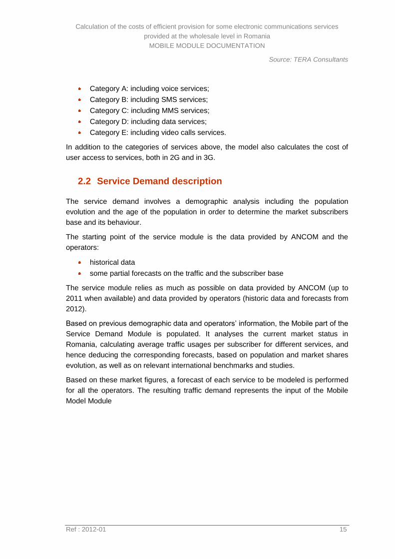
2.2 Service Demand description
The service demand involves a demographic analysis including the population
evolution and the age of the population in order to determine the market subscribers
base and its behaviour.
The starting point of the service module is the data provided by ANCOM and the
operators:
historical data
some partial forecasts on the traffic and the subscriber base
The service module relies as much as possible on data provided by ANCOM (up to
2011 when available) and data provided by operators (historic data and forecasts from
2012).
Based on previous demographic data and operators’ information, the Mobile part of the
Service Demand Module is populated. It analyses the current market status in
Romania, calculating average traffic usages per subscriber for different services, and
hence deducing the corresponding forecasts, based on population and market shares
evolution, as well as on relevant international benchmarks and studies.
Based on these market figures, a forecast of each service to be modeled is performed
for all the operators. The resulting traffic demand represents the input of the Mobile
Model Module
Calculation of the costs of efficient provision for some electronic communications services
provided at the wholesale level in Romania
MOBILE MODULE DOCUMENTATION
Ref : 2012-01 16
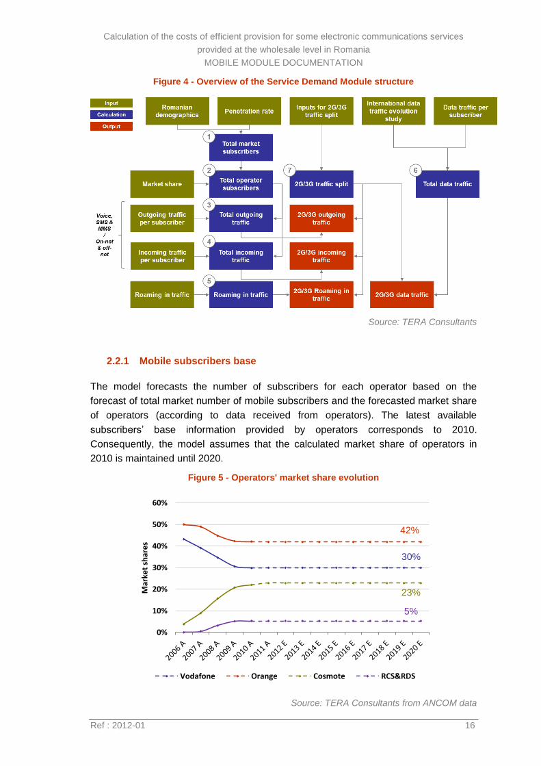
Figure 4 - Overview of the Service Demand Module structure
Source: TERA Consultants
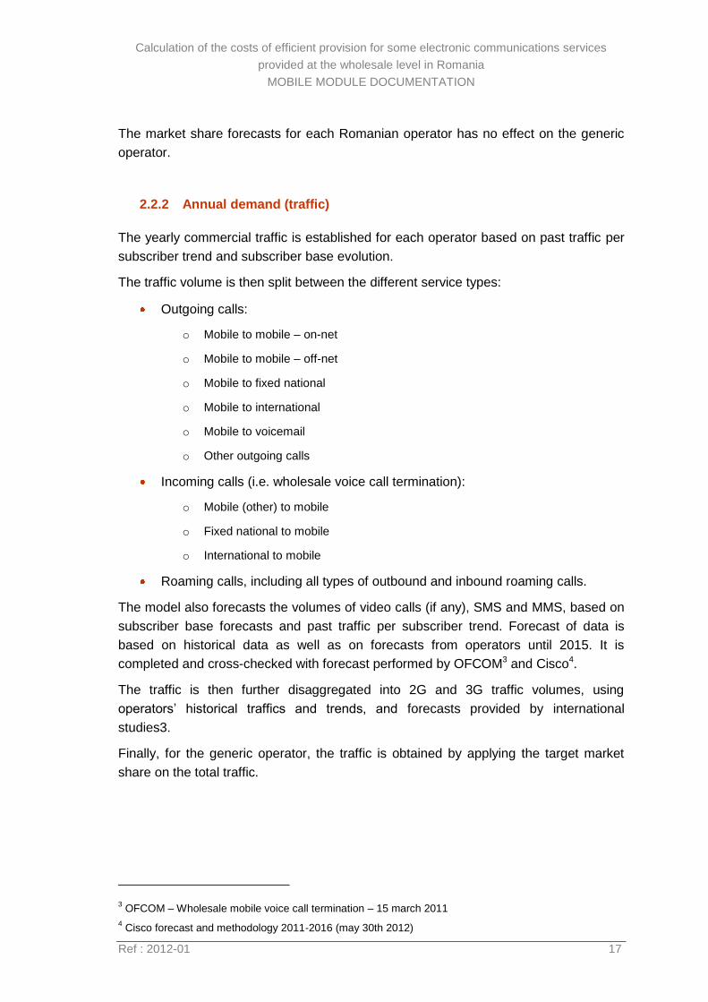
2.2.1 Mobile subscribers base
The model forecasts the number of subscribers for each operator based on the
forecast of total market number of mobile subscribers and the forecasted market share
of operators (according to data received from operators). The latest available
subscribers’ base information provided by operators corresponds to 2010.
Consequently, the model assumes that the calculated market share of operators in
2010 is maintained until 2020.
Figure 5 - Operators' market share evolution
Source: TERA Consultants from ANCOM data
0%
10%
20%
30%
40%
50%
60%
Mar
ket
shar
es
Vodafone Orange Cosmote RCS&RDS
42%
30%
23%
5%
Calculation of the costs of efficient provision for some electronic communications services
provided at the wholesale level in Romania
MOBILE MODULE DOCUMENTATION
Ref : 2012-01 17
The market share forecasts for each Romanian operator has no effect on the generic
operator.
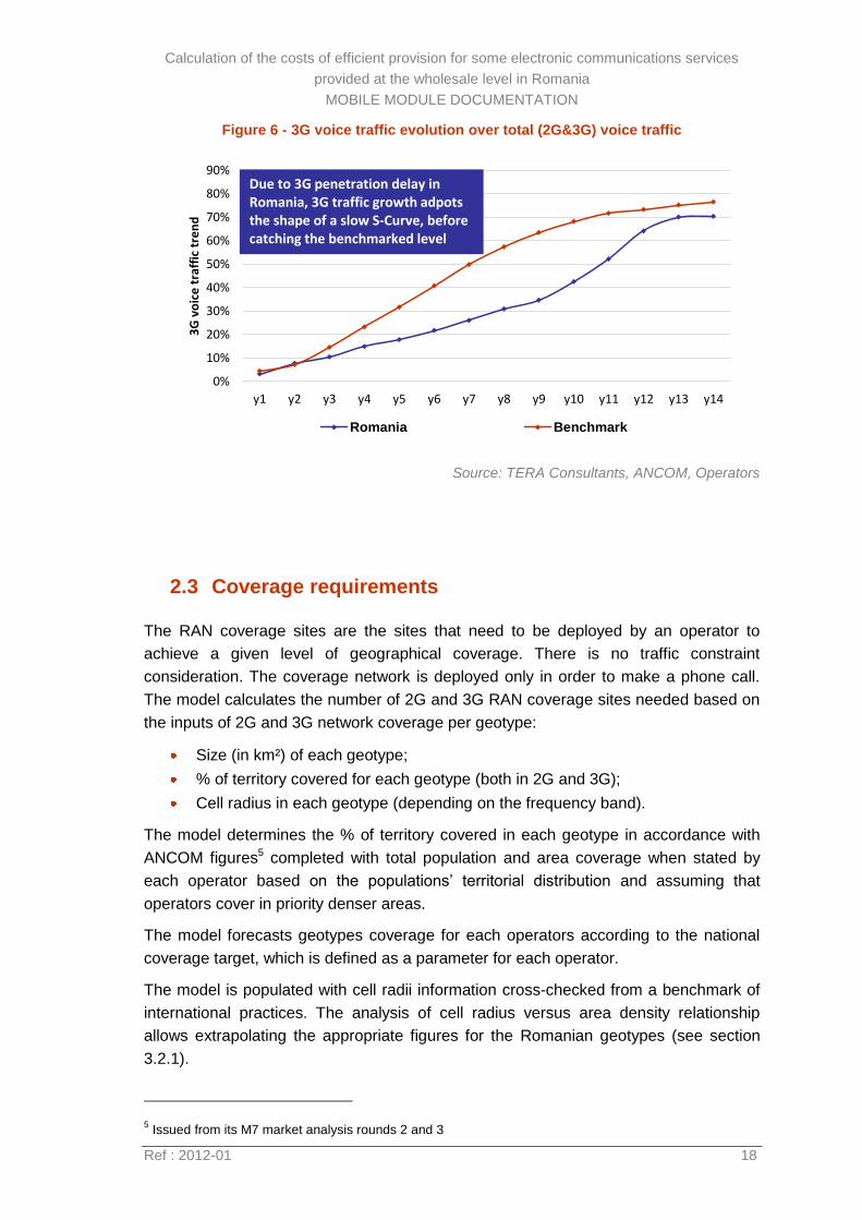
2.2.2 Annual demand (traffic)
The yearly commercial traffic is established for each operator based on past traffic per
subscriber trend and subscriber base evolution.
The traffic volume is then split between the different service types:
Outgoing calls:
o Mobile to mobile – on-net
o Mobile to mobile – off-net
o Mobile to fixed national
o Mobile to international
o Mobile to voicemail
o Other outgoing calls
Incoming calls (i.e. wholesale voice call termination):
o Mobile (other) to mobile
o Fixed national to mobile
o International to mobile
Roaming calls, including all types of outbound and inbound roaming calls.
The model also forecasts the volumes of video calls (if any), SMS and MMS, based on
subscriber base forecasts and past traffic per subscriber trend. Forecast of data is
based on historical data as well as on forecasts from operators until 2015. It is
completed and cross-checked with forecast performed by OFCOM3 and Cisco4.
The traffic is then further disaggregated into 2G and 3G traffic volumes, using
operators’ historical traffics and trends, and forecasts provided by international
studies3.
Finally, for the generic operator, the traffic is obtained by applying the target market
share on the total traffic.
3 OFCOM – Wholesale mobile voice call termination – 15 march 2011
4 Cisco forecast and methodology 2011-2016 (may 30th 2012)
Calculation of the costs of efficient provision for some electronic communications services
provided at the wholesale level in Romania
MOBILE MODULE DOCUMENTATION
Ref : 2012-01 18
Figure 6 - 3G voice traffic evolution over total (2G&3G) voice traffic
Source: TERA Consultants, ANCOM, Operators
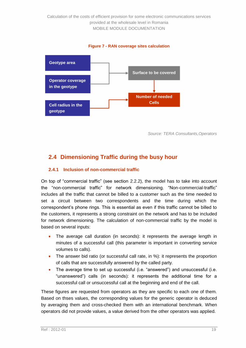
2.3 Coverage requirements
The RAN coverage sites are the sites that need to be deployed by an operator to
achieve a given level of geographical coverage. There is no traffic constraint
consideration. The coverage network is deployed only in order to make a phone call.
The model calculates the number of 2G and 3G RAN coverage sites needed based on
the inputs of 2G and 3G network coverage per geotype:
Size (in km²) of each geotype;
% of territory covered for each geotype (both in 2G and 3G);
Cell radius in each geotype (depending on the frequency band).
The model determines the % of territory covered in each geotype in accordance with
ANCOM figures5 completed with total population and area coverage when stated by
each operator based on the populations’ territorial distribution and assuming that
operators cover in priority denser areas.
The model forecasts geotypes coverage for each operators according to the national
coverage target, which is defined as a parameter for each operator.
The model is populated with cell radii information cross-checked from a benchmark of
international practices. The analysis of cell radius versus area density relationship
allows extrapolating the appropriate figures for the Romanian geotypes (see section
3.2.1).
5 Issued from its M7 market analysis rounds 2 and 3
0%
10%
20%
30%
40%
50%
60%
70%
80%
90%
y1 y2 y3 y4 y5 y6 y7 y8 y9 y10 y11 y12 y13 y14
3G
vo
ice
tra
ffic
tre
nd
Romania Benchmark
Due to 3G penetration delay in Romania, 3G traffic growth adpots the shape of a slow S-Curve, before catching the benchmarked level
Calculation of the costs of efficient provision for some electronic communications services
provided at the wholesale level in Romania
MOBILE MODULE DOCUMENTATION
Ref : 2012-01 19
Figure 7 - RAN coverage sites calculation
Source: TERA Consultants,Operators
2.4 Dimensioning Traffic during the busy hour
2.4.1 Inclusion of non-commercial traffic
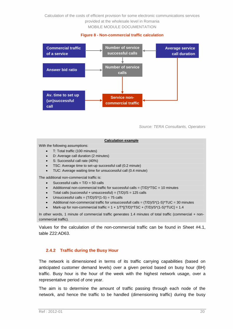
On top of “commercial traffic” (see section 2.2.2), the model has to take into account
the “non-commercial traffic” for network dimensioning. “Non-commercial-traffic”
includes all the traffic that cannot be billed to a customer such as the time needed to
set a circuit between two correspondents and the time during which the
correspondent’s phone rings. This is essential as even if this traffic cannot be billed to
the customers, it represents a strong constraint on the network and has to be included
for network dimensioning. The calculation of non-commercial traffic by the model is
based on several inputs:
The average call duration (in seconds): it represents the average length in
minutes of a successful call (this parameter is important in converting service
volumes to calls).
The answer bid ratio (or successful call rate, in %): it represents the proportion
of calls that are successfully answered by the called party.
The average time to set up successful (i.e. “answered”) and unsuccessful (i.e.
“unanswered”) calls (in seconds): it represents the additional time for a
successful call or unsuccessful call at the beginning and end of the call.
These figures are requested from operators as they are specific to each one of them.
Based on thses values, the corresponding values for the generic operator is deduced
by averaging them and cross-checked them with an international benchmark. When
operators did not provide values, a value derived from the other operators was applied.
Operator coverage
in the geotype
Cell radius in the
geotype
Surface to be covered
Geotype area
Number of needed
Cells
Calculation of the costs of efficient provision for some electronic communications services
provided at the wholesale level in Romania
MOBILE MODULE DOCUMENTATION
Ref : 2012-01 20
Figure 8 - Non-commercial traffic calculation
Source: TERA Consultants, Operators
Calculation example
With the following assumptions:
T: Total traffic (100 minutes)
D: Average call duration (2 minutes)
S: Successful call rate (40%)
TSC: Average time to set-up successful call (0.2 minute)
TUC: Average waiting time for unsuccessful call (0.4 minute)
The additional non-commercial traffic is:
Successful calls = T/D = 50 calls
Additionnal non-commercial traffic for successful calls = (T/D)*TSC = 10 minutes
Total calls (successful + unsuccessful) = (T/D)/S = 125 calls
Unsuccessful calls = (T/D)/S*(1-S) = 75 calls
Additional non-commercial traffic for unsuccessfull calls = (T/D)/S*(1-S)*TUC = 30 minutes
Mark-up for non-commercial traffic = 1 + 1/T*[(T/D)*TSC + (T/D)/S*(1-S)*TUC] = 1.4
In other words, 1 minute of commercial traffic generates 1.4 minutes of total traffic (commercial + non-
commercial traffic).
Values for the calculation of the non-commercial traffic can be found in Sheet #4.1,
table Z22:AD63.
2.4.2 Traffic during the Busy Hour
The network is dimensioned in terms of its traffic carrying capabilities (based on
anticipated customer demand levels) over a given period based on busy hour (BH)
traffic. Busy hour is the hour of the week with the highest network usage, over a
representative period of one year.
The aim is to determine the amount of traffic passing through each node of the
network, and hence the traffic to be handled (dimensioning traffic) during the busy
Average service
call duration
Answer bid ratio
Number of service
successful calls
Commercial traffic
of a service
Service non-
commercial traffic
Av. time to set up
(un)successful
call
Number of service
calls
Calculation of the costs of efficient provision for some electronic communications services
provided at the wholesale level in Romania
MOBILE MODULE DOCUMENTATION
Ref : 2012-01 21
hour. The ratio with each equipment capacity finally gives the number of equipment
required during the busy hour.
Equipment capacity is expressed either in Erlangs or in Mbps or in busy hour call
attempts (BHCA). The capacity of equipment whose constraints are relating to the
number of concurrent calls is usually expressed in Erlangs. Therefore, one Erlang
represents the continuous use of one voice path during a period of time (usually one
hour). Other equipment are dimensioned in terms of the maximum throughput they can
support in the busy hours. Their capacity is then expressed in Mbps. Finally, some
equipment are dimensioned in terms of the number of call attempts they handle during
the busy hour.
Consequently, all services (including voice, SMS6, MMS, video calls and data) traffic
must be converted to the appropriate unit: Erlangs, Mbps and BHCA.
The modeled network is separated into two main parts: RAN and Core. Transmitted
information evolves through these networks with different throughput, due to the
different modulation techniques used in each part. Therefore, the dimensioning traffic
(Mbps, Erlangs) is not the same in access network and in core network.
Equipment located in the access network (such as BTS, Node B, BSC …) are
dimensioned with access dimensioning traffic, while equipment situated in core network
(MSC, MGW …) are dimensioned with core dimensioning traffic.
Busy hour traffic is calculated based on busy hour traffic information provided for each
cell by operators, breaked down on a service basis (voice/data) and on technology
basis (2G/3G), and the trend of annual traffic of operators.
As voice services busy hour may differ from data services busy hour, the model does
not assume a full overlapping for voice and data BH, and introduces a BH traffic
reduction parameter which reflects that non-overlapping. In, fact, if voice and data BH
were identical, then the network should be dimensioned in order to support both voice
and data busy hour traffics at the same time. In that case the non-overlapping
parameter equals 100%. If voice BH differs from data BH, which is more likely to
correspond to reality, then the network is dimensioned with lower traffic constraints
since the highest constraint on voice does not happen in the same time that the highest
constraint on data. In the latter case, the non-overlapping parameter has a lower value
than 100%. In the model, that parameter is defined at a conservative value of 90% to
reflect the fact that the network is dimensioned by taking into account the maximum BH
voice and maximum BH data, not occurring at the same timeand is applied to BH traffic
going through each network node.
Finally, the calculated busy hour evolving through the RAN takes into account the
amount of traffic offloaded in the IBS (In-Building Solutions). In fact, the model defines
two off-load parameters for both 2G and 3G traffics, only for urban traffic. These
6 Although SMS traffic does not have a direct impact on radio site dimensioning, it does bear a share of the
costs of those radio sites
Calculation of the costs of efficient provision for some electronic communications services
provided at the wholesale level in Romania
MOBILE MODULE DOCUMENTATION
Ref : 2012-01 22
parameters are issued from an international benchmark and can be changed in the
model (no data was provided by operators). As a consequence, the busy hour traffic to
be supported by BTS/Node B equipment is relieved of 2G/3G IBS traffic.
Conversion rules for both access and core dimensioning traffic detailed in Appendix.
The final values for the traffic conversion can be found in Sheet #4.0, line 73 to 117.
Calculation of the costs of efficient provision for some electronic communications services
provided at the wholesale level in Romania
MOBILE MODULE DOCUMENTATION
Ref : 2012-01 23
3 Network dimensioning
Based on demand and engineering principles and algorithms, the model determines
the number of network elements required. This network dimensioning step calculates
the volume of network elements required to support the given level of demand during
the busy hour using the chosen technology.
As explained in the scope of the model (section 1.1), the network dimensioning is
divided into three main steps:
Radio access network dimensioning;
Core network dimensioning;
Transmission network dimensioning.
Before dimensioning the Radio Access Network, and after calculating the BH traffic for
each service, the model calculates first the amount of traffic circulating through each
network node. This traffic is function of the BH traffic for each service and how much
each service uses each network node (routing factor).
3.1 Routing matrix
The network routing matrix (or routing table) defines how each service uses the
network, i.e. how much of each network element is used by the service on average.
The full usage of the network by a network product may be based on the service’s
volume of minutes or data size or numbers of calls made or any other relevant driver.
This information is in a table that lists how much of each network element is used by
the product. The "how much" is the effective cost driver and can be numbers of
network elements, or relative cost usage (as long as the same cost driver is used for
each network element by each product, any driver may be used).
The model considers that the routing factors should be an estimate of the average
number of each type of network element used for each service. In the cases where
more than one possible route exists (e.g. at the core level), then the average number of
network elements used for each route is weighted by the probability that this route can
occur.
Each operator provided its routing table, considered as raw data. These routing tables
may differ in the list of equipment provided and in the routing factors corresponding to
the probability of the route. Hence, the routing tables provided by operators are treated
in order to have a global homogeneity between all operators, and to fit to the adopted
table format of the model.
The Routing table of the generic operator is given in Appendix 11.4. It is based on the
most relevant values for each equipment provided by operators, according to TERA
expertise.
Calculation of the costs of efficient provision for some electronic communications services
provided at the wholesale level in Romania
MOBILE MODULE DOCUMENTATION
Ref : 2012-01 24
The routing matrix for each operator can be found in Sheets #2.x, line 828 to 873
3.2 Radio Access Network dimensioning (Sheets 4.2 for 2G
and 4.3 for 3G)
Network dimensioning starts with estimating the radio network required to handle
demand (both geographic demand and traffic demand).
In order to achieve a certain level of geographic coverage, the areas covered by a
mobile network are divided into smaller areas called cells. Each cell is a unitary
network element which includes its own equipment in order to transmit, receive and
switch the calls from subscribers located within the borders of its radio coverage area.
The model assumes one main cell type for coverage, that is to say macrocells. For
macrocells, the base station antennas are installed on a mast or a pole (in a rural area)
or on top of a tall building (rooftop).
The objective of the model is to design a radio network configuration that meets the
required level of demand. To do this, the model incorporates the following
assumptions:
A network is rolled out to provide geographical coverage (i.e., there is only a
minimum level of traffic) by applying the cell radius and a scorched-node
coefficient7 (SNC).
Coverage sites are then considered equipped with maximum transceivers
configuration, as described in the following sections (3 sectors per BTS and 4 to
6 TRX8 per sector for 2G dimensioning, according to information provided by
operators).
If coverage sites with that configuration are sufficient to handle the demand
traffic, sites configuration is then optimized (less transceivers per site where
appropriate)
In the dual band networks, such as 2G 900-1800 or 3G 900-2100, transceivers
for each band are collocated at the same base stations and additional 2G 1800
transceivers (or 3G 900 and 2100 carriers and transceivers) and equipment are
added to provide additional traffic capacity. The upper limit on the number of
transceivers per base station is determined by either:
o The physical limit of the number of transceivers, which is a maximum of
4 to 6 transceivers per sector (based on operators data).
7 Because coverage of an area cannot be performed in an ideal way with a perfect hexagon paving, the
use of a SNC reflects the difficulty to display the sites in the best locations and the existence of blocking environments (big buildings) that reduces the coverage.
8 The number of TRX per sector is the minimum between the maximum number of TRX possible with
available spectrum, and the maximum number of TRX that is possible to put in the rack and based on operator’s inputs.
Calculation of the costs of efficient provision for some electronic communications services
provided at the wholesale level in Romania
MOBILE MODULE DOCUMENTATION
Ref : 2012-01 25
o The number of transceivers and carriers per sector that the spectrum
will allow. The model derives this from the spectrum allocations and, for
bands that can be used for both 2G and 3G, after allowing for any
allocation to either 2G or 3G.
Once each base station is fully configured with both 2G 900 and 1800
transceivers and 3G 900 and 2100 transceivers and carriers, additional base
stations are added to provide additional traffic capacity when needed.
2G and 3G networks for each existing operator are modeled as if it was entering the
market now at its current scale and scope of operation with a 2G and 3G network.
3.2.1 Main inputs
3.2.1.1 Spectrum and technology
Operators have frequency bandwidths in GMS 900 Mhz and 1800 Mhz (2G spectrum)
and in 3G spectrum (2100 Mhz). Frequency spectrum is divided in coupled channels
(duplex) for uplink and downlink.
In terms of functionality, 2G and 3G RAN equipment are quite similar: BTS/Node-B,
BSC/RNC; with enhanced capabilities for 3G equipment. In terms of technology, the
model considers the HSPA release of 3G (High Speed Packet Access) in combination
with 2G. It also includes a forward-looking network structure implementation, as
described in the following paragraphs.
Spectrum availability for each operator can vary over time and is to be found in Sheets
#2.x, line 368 to 384.
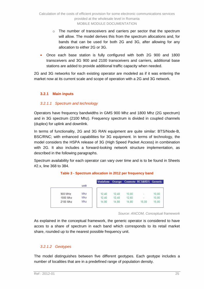
Table 3 - Spectrum allocation in 2012 per frequency band
Source: ANCOM, Conceptual framework
As explained in the conceptual framework, the generic operator is considered to have
acces to a share of spectrum in each band which corresponds to its retail market
share, rounded up to the nearest possible frequency unit.
3.2.1.2 Geotypes
The model distinguishes between five different geotypes. Each geotype includes a
number of localities that are in a predefined range of population density.
Calculation of the costs of efficient provision for some electronic communications services
provided at the wholesale level in Romania
MOBILE MODULE DOCUMENTATION
Ref : 2012-01 26
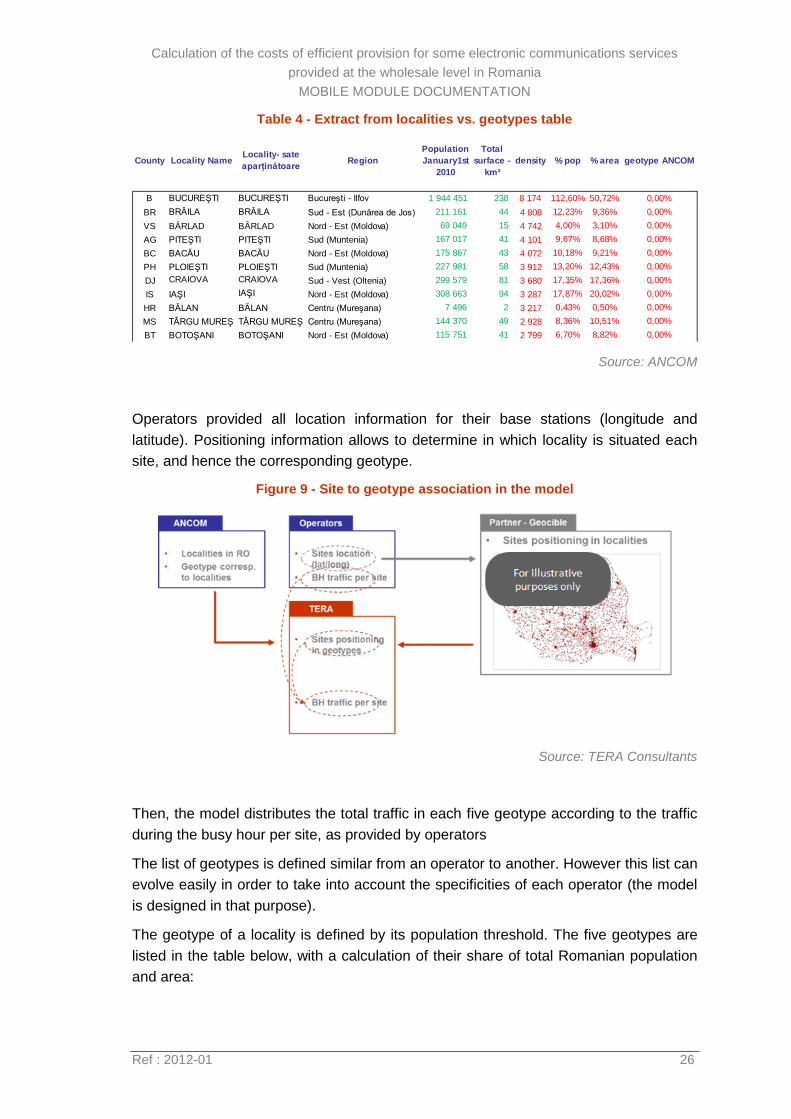
Table 4 - Extract from localities vs. geotypes table
Source: ANCOM
Operators provided all location information for their base stations (longitude and
latitude). Positioning information allows to determine in which locality is situated each
site, and hence the corresponding geotype.
Figure 9 - Site to geotype association in the model
Source: TERA Consultants
Then, the model distributes the total traffic in each five geotype according to the traffic
during the busy hour per site, as provided by operators
The list of geotypes is defined similar from an operator to another. However this list can
evolve easily in order to take into account the specificities of each operator (the model
is designed in that purpose).
The geotype of a locality is defined by its population threshold. The five geotypes are
listed in the table below, with a calculation of their share of total Romanian population
and area:
County Locality NameLocality- sate
aparţinătoareRegion
Population
January1st
2010
Total
surface -
km²
density % pop % area geotype ANCOM
B BUCUREŞTI BUCUREŞTI Bucureşti - Ilfov 1 944 451 238 8 174 112,60% 50,72% 0,00%
BR BRĂILA BRĂILA Sud - Est (Dunărea de Jos) 211 161 44 4 808 12,23% 9,36% 0,00%
VS BÂRLAD BÂRLAD Nord - Est (Moldova) 69 049 15 4 742 4,00% 3,10% 0,00%
AG PITEŞTI PITEŞTI Sud (Muntenia) 167 017 41 4 101 9,67% 8,68% 0,00%
BC BACĂU BACĂU Nord - Est (Moldova) 175 867 43 4 072 10,18% 9,21% 0,00%
PH PLOIEŞTI PLOIEŞTI Sud (Muntenia) 227 981 58 3 912 13,20% 12,43% 0,00%
DJ CRAIOVA CRAIOVA Sud - Vest (Oltenia) 299 579 81 3 680 17,35% 17,36% 0,00%
IS IAŞI IAŞI Nord - Est (Moldova) 308 663 94 3 287 17,87% 20,02% 0,00%
HR BĂLAN BĂLAN Centru (Mureşana) 7 496 2 3 217 0,43% 0,50% 0,00%
MS TÂRGU MUREŞ TÂRGU MUREŞ Centru (Mureşana) 144 370 49 2 928 8,36% 10,51% 0,00%
BT BOTOŞANI BOTOŞANI Nord - Est (Moldova) 115 751 41 2 799 6,70% 8,82% 0,00%
Calculation of the costs of efficient provision for some electronic communications services
provided at the wholesale level in Romania
MOBILE MODULE DOCUMENTATION
Ref : 2012-01 27
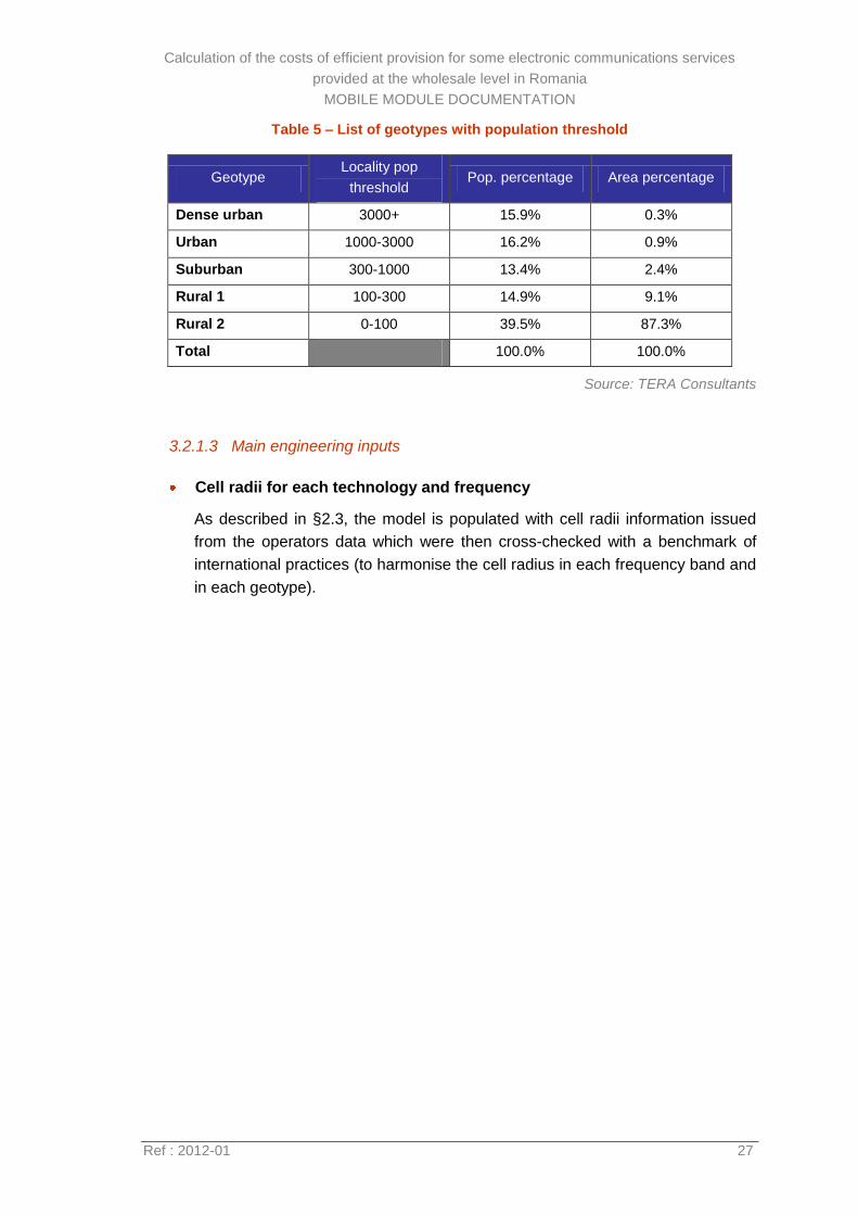
Table 5 – List of geotypes with population threshold
Geotype Locality pop
threshold Pop. percentage Area percentage
Dense urban 3000+ 15.9% 0.3%
Urban 1000-3000 16.2% 0.9%
Suburban 300-1000 13.4% 2.4%
Rural 1 100-300 14.9% 9.1%
Rural 2 0-100 39.5% 87.3%
Total 100.0% 100.0%
Source: TERA Consultants
3.2.1.3 Main engineering inputs
Cell radii for each technology and frequency
As described in §2.3, the model is populated with cell radii information issued
from the operators data which were then cross-checked with a benchmark of
international practices (to harmonise the cell radius in each frequency band and
in each geotype).
Calculation of the costs of efficient provision for some electronic communications services
provided at the wholesale level in Romania
MOBILE MODULE DOCUMENTATION
Ref : 2012-01 28
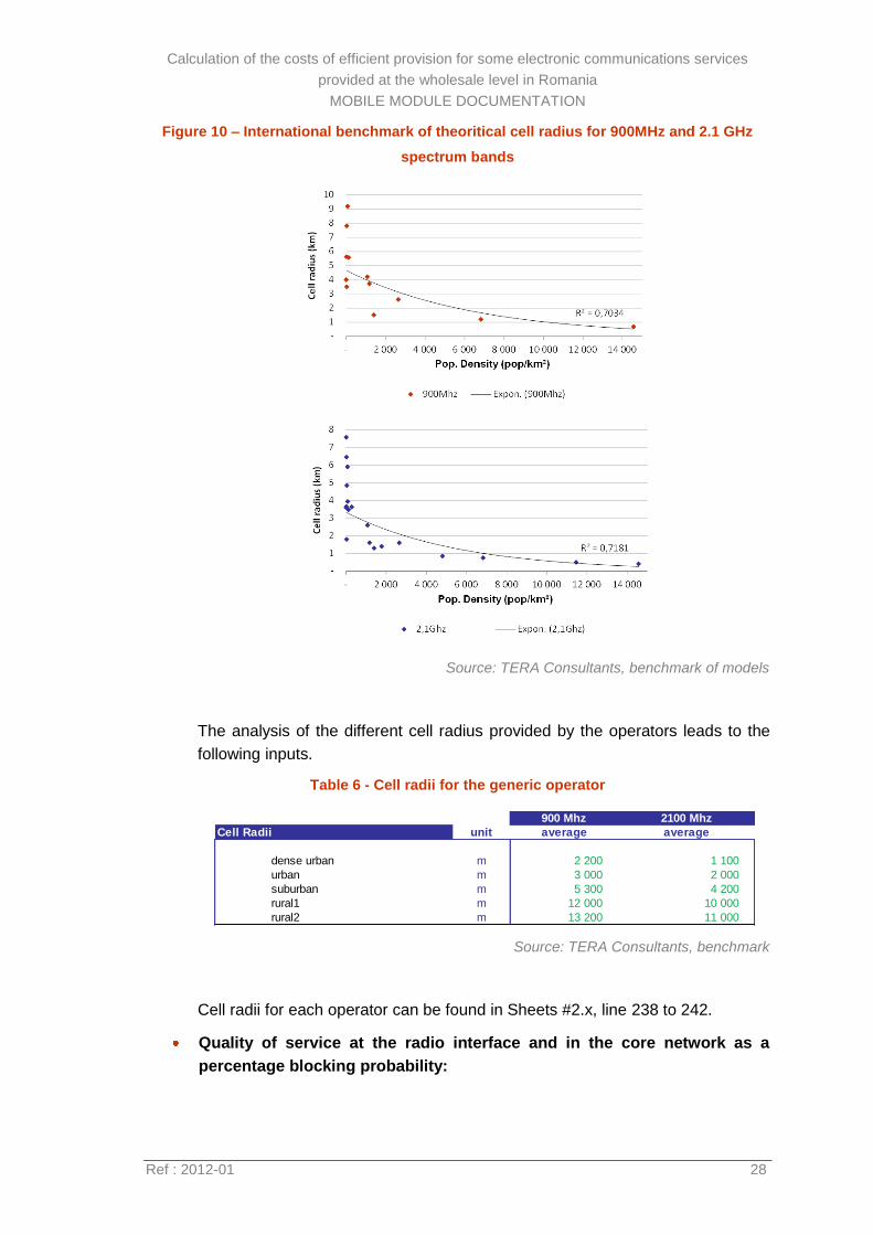
Figure 10 – International benchmark of theoritical cell radius for 900MHz and 2.1 GHz
spectrum bands
Source: TERA Consultants, benchmark of models
The analysis of the different cell radius provided by the operators leads to the
following inputs.
Table 6 - Cell radii for the generic operator
Source: TERA Consultants, benchmark
Cell radii for each operator can be found in Sheets #2.x, line 238 to 242.
Quality of service at the radio interface and in the core network as a
percentage blocking probability:
Cell Radii unit average average
dense urban m 2 200 1 100
urban m 3 000 2 000
suburban m 5 300 4 200
rural1 m 12 000 10 000
rural2 m 13 200 11 000
900 Mhz 2100 Mhz
Calculation of the costs of efficient provision for some electronic communications services
provided at the wholesale level in Romania
MOBILE MODULE DOCUMENTATION
Ref : 2012-01 29
The blocking probability is the network design call failure rate in the busy hour.
The relevant column of the Erlang B table (see below) is calculated from the
blocking probability.
Call blocking probability can be found in Sheets #2.x, line 866.
Number of total channels per 2G TRX
Basically 8 channels per TRX as well as the number of channels reserved for
signaling. Their difference will be the number of channel allocated to voice.
The number of channels per TRX, and the corresponding number of maximum
simultaneous communications are calculated for the generic operator as
average of other operators’ values.
Number of total channels per 2G TRX can be found in Sheets #2.x, line 308 to
327.
Number of total channel elements per 3G carriers
Pole capacity channels (CE pool) are considered for dimensioning. The size of
CE pool is provided by operators and cross-checked with a benchmark of public
available models in Europe and Middle East: 64 CE for uplink and 64 CE for
downlink per carrier per site for the generic operator.
Pole capacity can be found in Sheets #2.x, line 337.
RNC soft handover percentage
This is a characteristic of the 3G network which is related to the fact that each
subscriber while making a call may be connected to two or more cell sectors
that belong to the same physical cell site.
RNC soft handover percentage based on operators’ submission can be found in
Sheets #4.0, line 155.
Frequency reuse factor
Further detailed in coming paragraphs, it allows determining the frequency
reuse pattern. Considering 3 sectors per cell, and hexagonal cell shapes, the
frequency reuse factor is assumed to be equal to 12.
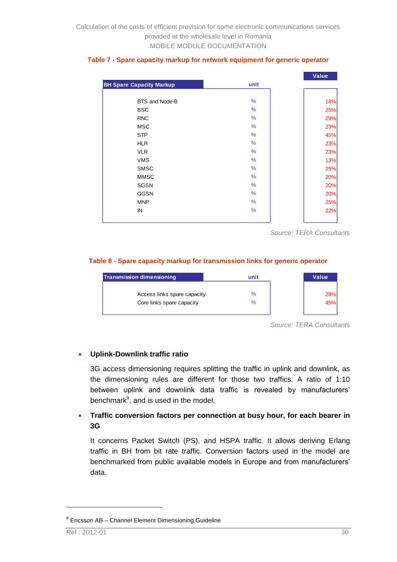
Spare capacity markup
Also known as security markup, it is applied on busy hour traffic, in order to
prevent from network saturation. It is requested from operators, and is provided
for the different network nodes.
Spare capacity mark-up can be found in Sheets #2.x, line 214 to 230 for
network equipment, and line 682 to 683 for transmission links.
The values for the generic operator are calculated as average of other
operators’ values:
Calculation of the costs of efficient provision for some electronic communications services
provided at the wholesale level in Romania
MOBILE MODULE DOCUMENTATION
Ref : 2012-01 30
Table 7 - Spare capacity markup for network equipment for generic operator
Source: TERA Consultants
Table 8 - Spare capacity markup for transmission links for generic operator
Source: TERA Consultants
Uplink-Downlink traffic ratio
3G access dimensioning requires splitting the traffic in uplink and downlink, as
the dimensioning rules are different for those two traffics. A ratio of 1:10
between uplink and downlink data traffic is revealed by manufacturers’
benchmark9, and is used in the model.
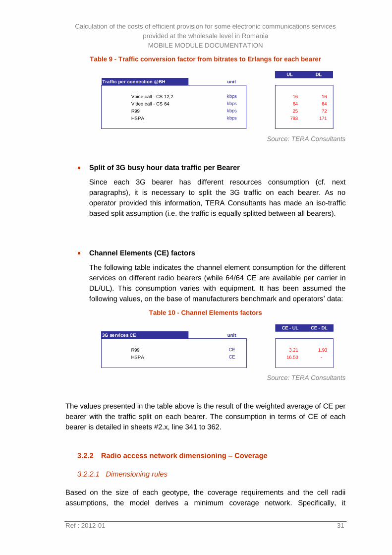
Traffic conversion factors per connection at busy hour, for each bearer in
3G
It concerns Packet Switch (PS), and HSPA traffic. It allows deriving Erlang
traffic in BH from bit rate traffic. Conversion factors used in the model are
benchmarked from public available models in Europe and from manufacturers’
data.
9 Ericsson AB – Channel Element Dimensioning Guideline
Value
BH Spare Capacity Markup unit
BTS and Node-B % 18%
BSC % 25%
RNC % 29%
MSC % 23%
STP % 45%
HLR % 23%
VLR % 23%
VMS % 13%
SMSC % 25%
MMSC % 20%
SGSN % 20%
GGSN % 20%
MNP % 25%
IN % 22%
Transmission dimensioning unit Value
Access links spare capacity % 28%
Core links spare capacity % 45%
Calculation of the costs of efficient provision for some electronic communications services
provided at the wholesale level in Romania
MOBILE MODULE DOCUMENTATION
Ref : 2012-01 31
Table 9 - Traffic conversion factor from bitrates to Erlangs for each bearer
Source: TERA Consultants
Split of 3G busy hour data traffic per Bearer
Since each 3G bearer has different resources consumption (cf. next
paragraphs), it is necessary to split the 3G traffic on each bearer. As no
operator provided this information, TERA Consultants has made an iso-traffic
based split assumption (i.e. the traffic is equally splitted between all bearers).
Channel Elements (CE) factors
The following table indicates the channel element consumption for the different
services on different radio bearers (while 64/64 CE are available per carrier in
DL/UL). This consumption varies with equipment. It has been assumed the
following values, on the base of manufacturers benchmark and operators’ data:
Table 10 - Channel Elements factors
Source: TERA Consultants
The values presented in the table above is the result of the weighted average of CE per
bearer with the traffic split on each bearer. The consumption in terms of CE of each
bearer is detailed in sheets #2.x, line 341 to 362.
3.2.2 Radio access network dimensioning – Coverage
3.2.2.1 Dimensioning rules
Based on the size of each geotype, the coverage requirements and the cell radii
assumptions, the model derives a minimum coverage network. Specifically, it
UL DL
Traffic per connection @BH unit
Voice call - CS 12,2 kbps 16 16
Video call - CS 64 kbps 64 64
R99 kbps 25 72
HSPA kbps 793 171
CE - UL CE - DL
unit
R99 CE 3.21 1.93
HSPA CE 16.50 -
3G services CE
Calculation of the costs of efficient provision for some electronic communications services
provided at the wholesale level in Romania
MOBILE MODULE DOCUMENTATION
Ref : 2012-01 32
determines the number of base stations required to provide coverage to each geotype
to enable a voice call.
Calculation example
With the following assumptions:
A: Area to be covered (100 km²)
R: Radius of a site (2 km)
SNC: scorched-node coefficient (0.8)
The number of coverage site is:
Number of sites = A / Area of an hexagon = A / [3*3^(1/2)*(R*SNC)²/2] = 13 sites
It is important to note that the costs of the minimum coverage network represents a
common cost which is thus distributed to all services in a LRAIC+ cost allocation, but
has no impact on voice call termination in case of a “pure LRIC” cost allocation for
wholesale voice call termination.
3.2.2.2 Results for the generic operator
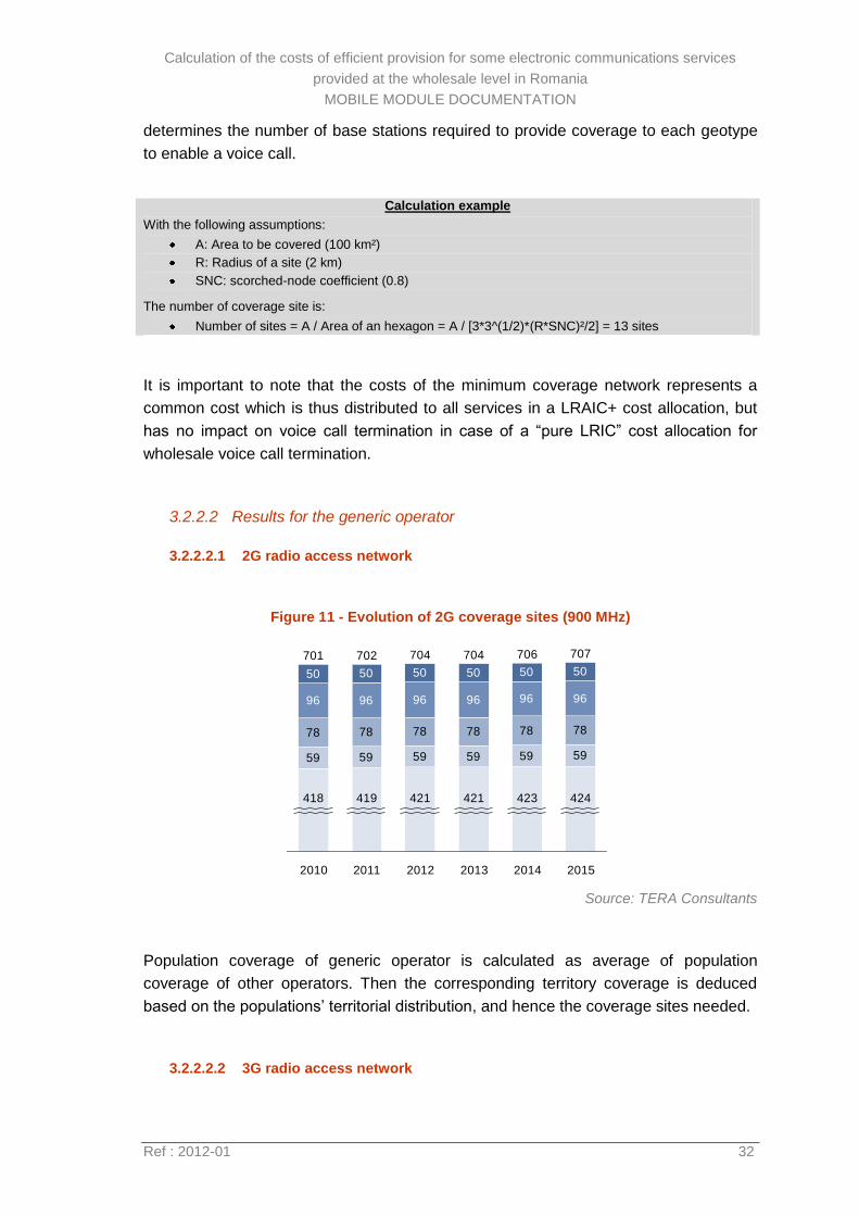
3.2.2.2.1 2G radio access network
Figure 11 - Evolution of 2G coverage sites (900 MHz)
Source: TERA Consultants
Population coverage of generic operator is calculated as average of population
coverage of other operators. Then the corresponding territory coverage is deduced
based on the populations’ territorial distribution, and hence the coverage sites needed.
3.2.2.2.2 3G radio access network
59 59 59 59 59 59 59 59 59 59
78 78 78 78 78 78 78 78 78 78
96 96 96 96 96 96 96 96 96 96
50 50 50 50 50 50 50 50 50 50
701
418
697 701
418
2008
700
417
2007
699
2009
416
2006
414rural2
rural1
suburban
urban
dense urban
2015
707
424
2014
706
423
2013
704 704
421
2012
421
2011
702
419
2010
Calculation of the costs of efficient provision for some electronic communications services
provided at the wholesale level in Romania
MOBILE MODULE DOCUMENTATION
Ref : 2012-01 33
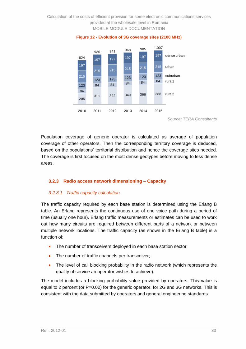
Figure 12 - Evolution of 3G coverage sites (2100 MHz)
Source: TERA Consultants
Population coverage of generic operator is calculated as average of population
coverage of other operators. Then the corresponding territory coverage is deduced,
based on the populations’ territorial distribution and hence the coverage sites needed.
The coverage is first focused on the most dense geotypes before moving to less dense
areas.
3.2.3 Radio access network dimensioning – Capacity
3.2.3.1 Traffic capacity calculation
The traffic capacity required by each base station is determined using the Erlang B
table. An Erlang represents the continuous use of one voice path during a period of
time (usually one hour). Erlang traffic measurements or estimates can be used to work
out how many circuits are required between different parts of a network or between
multiple network locations. The traffic capacity (as shown in the Erlang B table) is a
function of:
The number of transceivers deployed in each base station sector;
The number of traffic channels per transceiver;
The level of call blocking probability in the radio network (which represents the
quality of service an operator wishes to achieve).
The model includes a blocking probability value provided by operators. This value is
equal to 2 percent (or P=0.02) for the generic operator, for 2G and 3G networks. This is
consistent with the data submitted by operators and general engineering standards.
205311 322 349 366 388
84
84 84 84 84 84
123
123
123 123 123 123 123
125
215
215
215
215 215 215 215 215
197
197197
197
197 197 197 197 197
77
114
2007
322
2006 2010
824
2009 2014
985
2013
968
rural2
rural1
suburban
2008
489
dense urban
2015
1.007
565
30
2012
941
2011
930
urban
Calculation of the costs of efficient provision for some electronic communications services
provided at the wholesale level in Romania
MOBILE MODULE DOCUMENTATION
Ref : 2012-01 34
3.2.3.2 Utilisation factors
Although the radio access network is dimensioned based on the traffic during the busy
hour, the model has to take into account the fact that operators dimensioned their
network with a medium-term approach in order to better cope and anticipate site
densification needs, such as those driven by any unexpected surge of traffic.
A “utilisation factor” is thus added for the radio access network dimensioning on top of
the spare-capacity mark-ups. The spare capacity mark-up has been kept in the model,
the rationale being that the spare capacity mark-up is a macro strategic planning
parameter whereas the utilisation factor is a micro technical engineering parameter.
The RAN usage factor is thus a technical input and not a free parameter, whose value
can vary between 0% and 100% for each geotype and for each 2G and 3G RAN and
has the effect to increase the dimensioning traffic for the RAN. (see section § 3.2.1.3):
As no data was submitted on the utilisation factor used by the operators, the Model
relies on a calibration of the utilisation factors based on the current number of sites for
each operator.
The RAN usage factor is deduced from the “real” traffic and the “real” network of the
operator so it is calculated only once In fact it should have been an input by the
operators, not a calculation by the model (. This is performed through a macro
calibration (see Sheets in Sheets #2.x
3.2.3.3 Erlang B table
This table provides the amount of traffic for a given blocking probability and number of
available channels and is based upon statistical engineering calculations. It is used to
convert capacities from circuits to Erlangs or the opposite. For example, it has been
used in order to estimate the BTS capacity in Erlangs when the number of channels is
known.
3.2.3.4 Frequency reuse patterns
In theory, all cells can use the same carriers. This gives the advantage of allowing
more calls to be made at the same time. However, as the spectrum is narrow, this may
lead to interferences between the cells. Therefore, a spectrum reuse parameter is
introduced. It is function of the number of sectors per site.
The graph below shows an example:
Calculation of the costs of efficient provision for some electronic communications services
provided at the wholesale level in Romania
MOBILE MODULE DOCUMENTATION
Ref : 2012-01 35
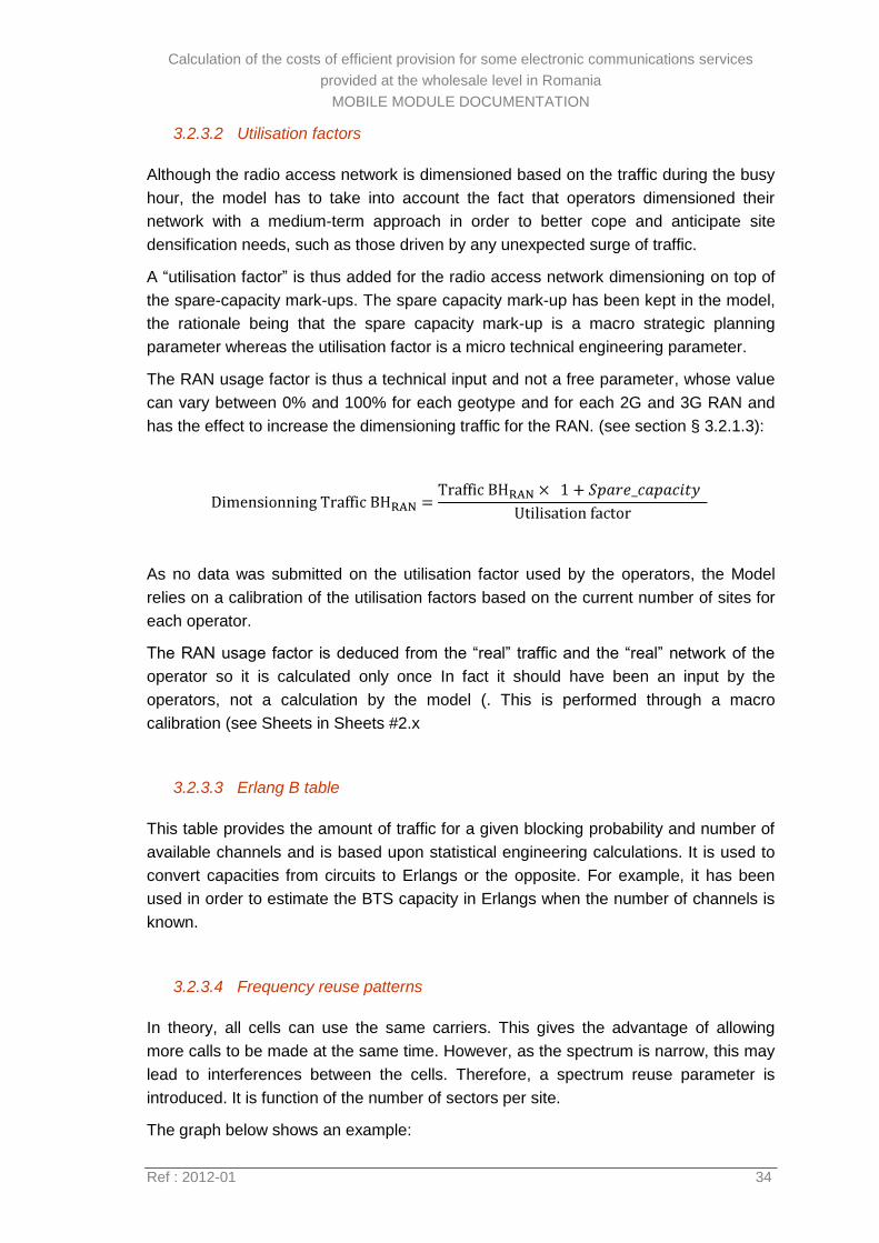
Figure 13 – Frequency reuse pattern of 3x4=12
Source: TERA Consultants
To determine the reuse pattern, the coverage area is represented in a set of
contiguous hexagons, to depict base station sites. Each site is split into 3 sectors. The
model assumes a frequency reuse pattern of 12, which allows at least one sector gap
between cells that use the same frequency11. This is equivalent to a base station
frequency reuse of four (assuming three sectors per base station).
The model further assumes that each 2G TRX requires 200 kHz of paired spectrum
and provides eight 25 kHz communication channels. For 3G, the model assumes that a
carrier requires 5 MHz and can carry 64 communication channels.
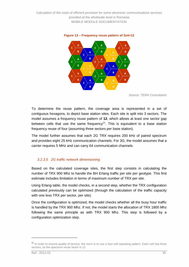
3.2.3.5 2G traffic network dimensioning
Based on the calculated coverage sites, the first step consists in calculating the
number of TRX 900 Mhz to handle the BH Erlang traffic per site per geotype. This first
estimate includes limitation in terms of maximum number of TRX per site.
Using Erlang table, the model checks, in a second step, whether the TRX configuration
calculated previously can be optimized (through the calculation of the traffic capacity
with one less TRX per sector, per site).
Once the configuration is optimized, the model checks whether all the busy hour traffic
is handled by the TRX 900 Mhz. If not, the model starts the allocation of TRX 1800 Mhz
following the same principle as with TRX 900 Mhz. This step is followed by a
configuration optimization step.
11 In order to ensure quality of service, the norm is to use a four-cell repeating pattern. Each cell has three
sectors, so the spectrum reuse factor is 12
A
B
C
A
B
C
A
B
C
A
B
C
A
B
C
A
B
C
A
B
C
A
B
C
A
B
C
A
B
C
A
B
C
A
B
C
A
B
C
A
B
C
A
B
C
Calculation of the costs of efficient provision for some electronic communications services
provided at the wholesale level in Romania
MOBILE MODULE DOCUMENTATION
Ref : 2012-01 36
Figure 14 - 2G TRX traffic dimensioning
Source: TERA Consultants
3.2.3.6 3G traffic network dimensioning
Based on the number of coverage 3G sites needed, the first step consists in calculating
the BH traffic per sector per site for each class of service (voice, video call in CS, data
in PS, and data in HSPA). While both voice and data was mixed to dimension 2G RAN
in terms of traffic, the split between service bearers is necessary in 3G, since each
service has a different traffic capacity consumption (also called channel element factor
or weight, as described in §3.2.1.3). Because channel elements consumption is
different in uplink and downlink, the BH traffic is also split between uplink and downlink,
for each class of service.
One way to dimension 3G RAN is to focus on voice dimensioning (Channel Switch
traffic) and service quality (GoS). This approach assumes that voice traffic is a priority
and hence the dimensioning is based on peak hour voice traffic, and blocking
probability parameter for service quality.
The model implements this approach and complements the 3G RAN dimensioning by a
second approach involving both of voice and data in their average traffic in BH (packet
switch traffic), and hence without quality of service consideration for voice (without
Erlang table).
Erlang B table
# of needed
TRX900 Mhz per
site per geotype
BH traffic per site
per geotype
3 sectors per site
Optimization
Number of
coverage sites Remaining non-
supported traffic?
# of needed
TRX1800 Mhz per
site per geotype
Optimization
Total number of
TRX
QoS: Cell blocking
probability
# needed sites
with 1800Mhz TRX
full config.
Traffic capacity
per site in
1800Mhz (full
config)
Calculation of the costs of efficient provision for some electronic communications services
provided at the wholesale level in Romania
MOBILE MODULE DOCUMENTATION
Ref : 2012-01 37
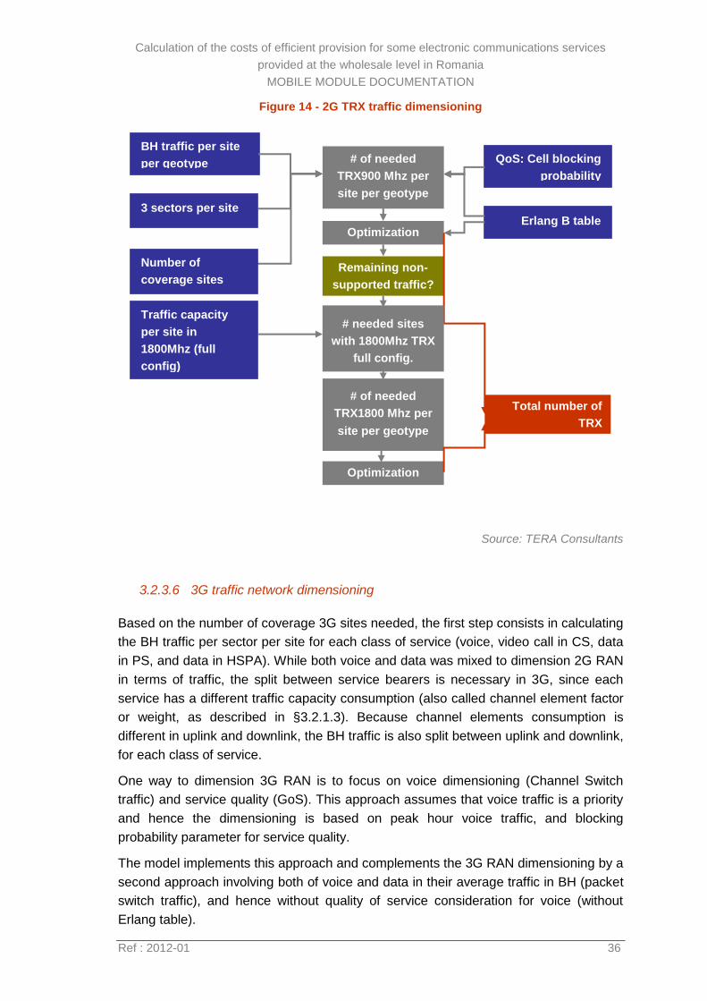
The model considers the maximum number of channel elements (CE) required for each
approach. The result is a number of CE per site per governorate. The following figure
summarizes the 3G RAN dimensioning process:
Figure 15 - Channel Element calculation algorithm (this figure represents the downlink
calculation but a similar calculation applies for uplink dimensioning)
Source: TERA Consultants
The same process is used for UL channel elements calculation. The three main steps
of the calculation aim to determine the following intermediary number of channel
elements:
#CE peak: it corresponds to the number of channel elements to handle peak
traffic in busy hour. It is function of the number of simultaneous users per site
for the service, and the channel element factor for the radio bearer
#CE average: When conversational and best effort bearers are mixed, the
dimensioning has to take the average traffic into consideration. As the
conversational traffic has higher priority, the interactive traffic will fill up space
when the conversational class traffic is not being used.
#CE best effort: based on the offered best effort traffic in Erlang for the service.
Once the number of required CE calculated, the models checks whether the number of
available carriers fulfills the need in terms of CE (64 CE per 5 Mhz bandwidth carrier for
the generic operator). If the number of available channel elements is not sufficient, the
model goes through the final step of densification.
MA
X
#CE peak traffic
DL
#CE average
traffic DL
#CE best effort
traffic DL
#CE for DL
∑
1st
approach
2nd
approach
Calculation of the costs of efficient provision for some electronic communications services
provided at the wholesale level in Romania
MOBILE MODULE DOCUMENTATION
Ref : 2012-01 38
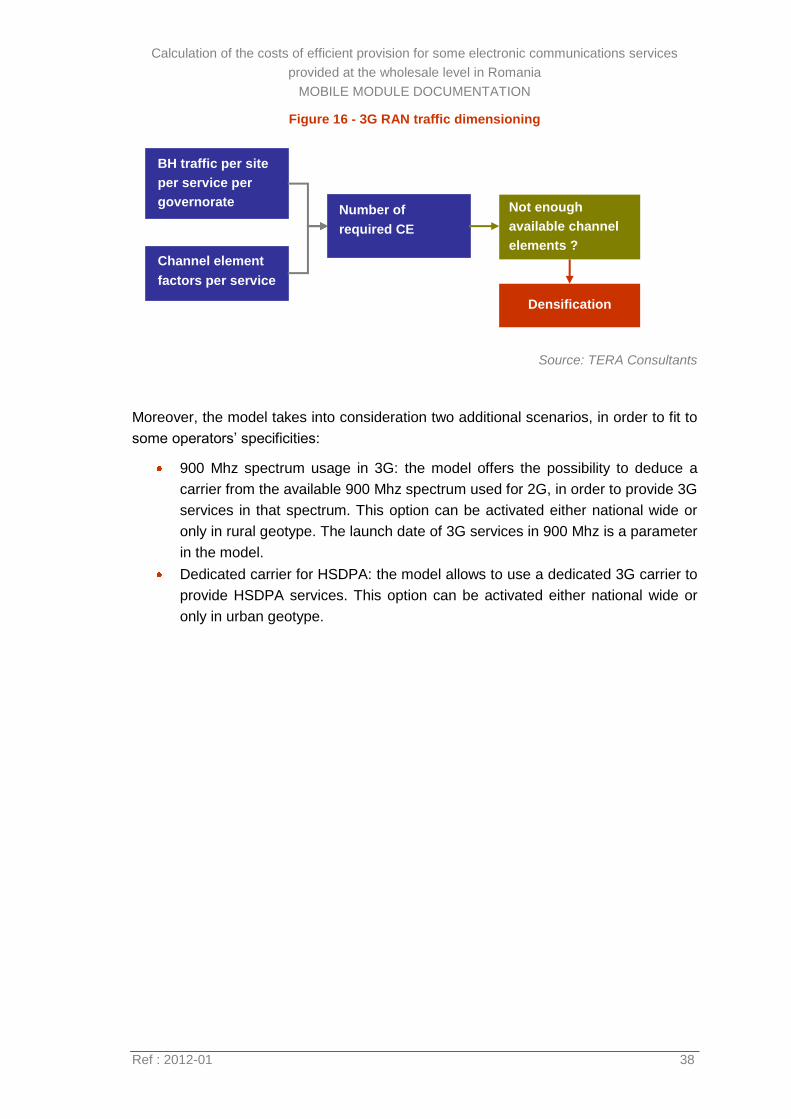
Figure 16 - 3G RAN traffic dimensioning
Source: TERA Consultants
Moreover, the model takes into consideration two additional scenarios, in order to fit to
some operators’ specificities:
900 Mhz spectrum usage in 3G: the model offers the possibility to deduce a
carrier from the available 900 Mhz spectrum used for 2G, in order to provide 3G
services in that spectrum. This option can be activated either national wide or
only in rural geotype. The launch date of 3G services in 900 Mhz is a parameter
in the model.
Dedicated carrier for HSDPA: the model allows to use a dedicated 3G carrier to
provide HSDPA services. This option can be activated either national wide or
only in urban geotype.
BH traffic per site
per service per
governorate
Channel element
factors per service
Densification
Number of
required CE
Not enough
available channel
elements ?
Calculation of the costs of efficient provision for some electronic communications services
provided at the wholesale level in Romania
MOBILE MODULE DOCUMENTATION
Ref : 2012-01 39
3.2.3.7 Results for the generic operator
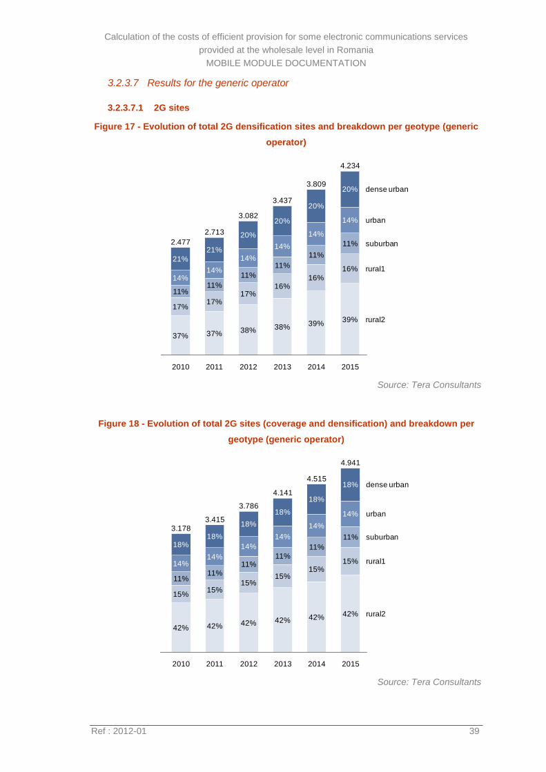
3.2.3.7.1 2G sites
Figure 17 - Evolution of total 2G densification sites and breakdown per geotype (generic
operator)
Source: Tera Consultants
Figure 18 - Evolution of total 2G sites (coverage and densification) and breakdown per
geotype (generic operator)
Source: Tera Consultants
dense urban
2015
11%
20%
2014
4.234
20%
16%
11%
14%
14%
16%
39%
3.437
2013
3.809
39%
21%
2009
1.954
35%
17%
11%
14%
22%
2008
1.215
31%
19%38%
16%
11%
14%
20%
2012
3.082
38%
17%
11%
14%
20%
2011
2.713
37%
17%
11%
14%
21%
2010
2.477
urban
17%
11%
14%
24%
2007
37%
22%
29%
2006
267
rural2
rural1
suburban
664
42%
15%
11%
14%
18%
2009
2.655
42%
15%
11%
14%
18%
964
dense urban
urban
rural1
suburban
rural2
2008
1.915
42%
15%
42%
18%
2007
1.363
15%
18%
43%
2015
4.941
42%
15%
11%
14%
18%
2014
4.515
42%
15%
11%
14%
18%
2013
4.141
42%
15%
11%
14%
18%
2012
3.786
42%
15%
11%
14%
18%
2011
3.415
42%
15%
11%
14%
18%
2010
3.178
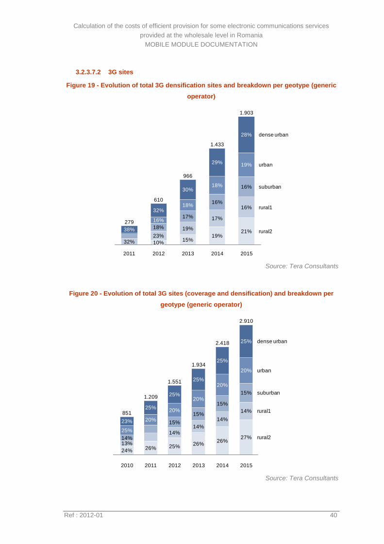
Calculation of the costs of efficient provision for some electronic communications services
provided at the wholesale level in Romania
MOBILE MODULE DOCUMENTATION
Ref : 2012-01 40
3.2.3.7.2 3G sites
Figure 19 - Evolution of total 3G densification sites and breakdown per geotype (generic
operator)
Source: Tera Consultants
Figure 20 - Evolution of total 3G sites (coverage and densification) and breakdown per
geotype (generic operator)
Source: Tera Consultants
suburban
urban
dense urban
1.903
21%
16%
16%
19%
28%
1.433
19%
17%
16%
18%
29%
966
15%
rural1
17%
18%
30%
2011
610
10%
23%
18%
16%
32%
2012
279
2015
32%
38%
2013 2014
rural219%
114
25%
23%
2008
489
40%
2007
14%
15%
20%
25%
2011
1.209
26%
20%
25%
2010
20%
25%
2013
1.934
26%
14%
15%
20%
25%
2012
1.551
25%
rural2
suburban
rural1
urban
dense urban
2009
322
61%
5%
35%
851
2015
2.910
27%
14%
15%
20%
25%
565
2.418
26%
14%
15%
24%
13%14%
2014
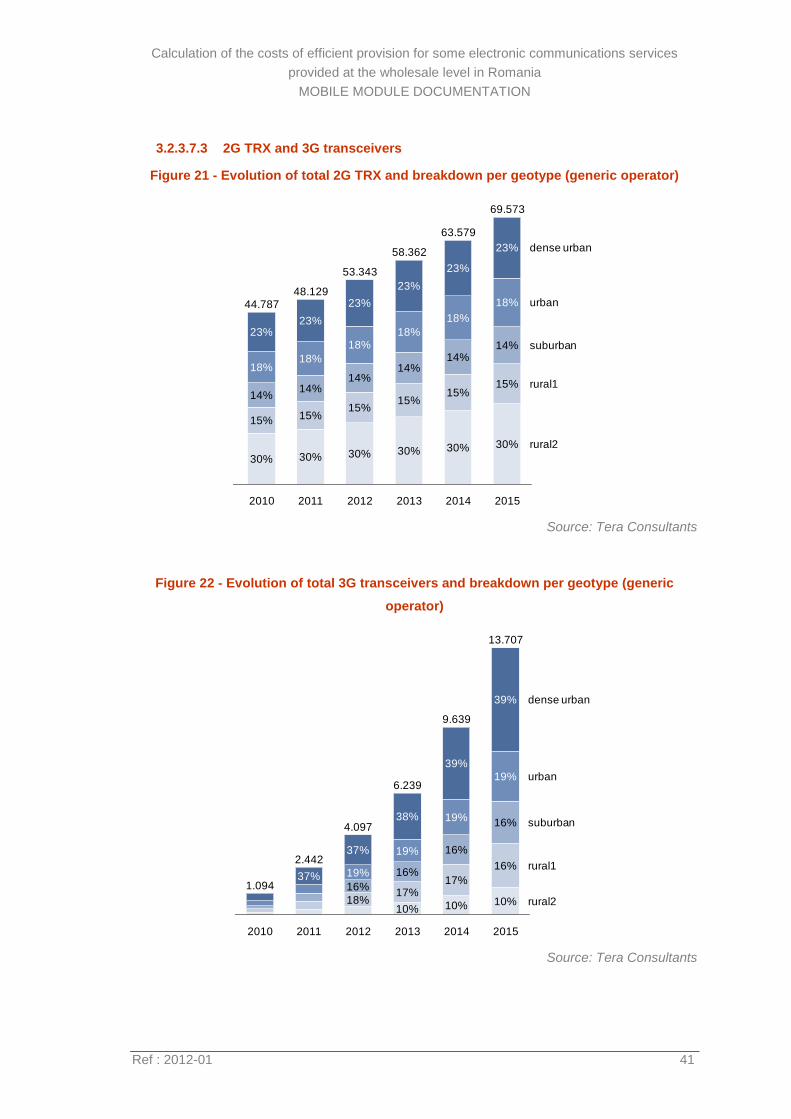
Calculation of the costs of efficient provision for some electronic communications services
provided at the wholesale level in Romania
MOBILE MODULE DOCUMENTATION
Ref : 2012-01 41
3.2.3.7.3 2G TRX and 3G transceivers
Figure 21 - Evolution of total 2G TRX and breakdown per geotype (generic operator)
Source: Tera Consultants
Figure 22 - Evolution of total 3G transceivers and breakdown per geotype (generic
operator)
Source: Tera Consultants
30%
15%
14%
18%
23%
2009
37.422
30%
15%
14%
18%
23%
13.284
dense urban
urban
rural1
suburban
rural2
2008
26.994
30%
15%
30%
23%
2007
19.215
15%
23%
30%
2015
69.573
30%
15%
14%
18%
23%
2014
63.579
30%
15%
14%
18%
23%
2013
58.362
30%
15%
14%
18%
23%
2012
53.343
30%
15%
14%
18%
23%
2011
48.129
30%
15%
14%
18%
23%
2010
44.787
11
19%
39%
2013
6.239
10%
17%
16%
19%
38%
2012
4.097
18%
16%
19%
37%
2011
2.442
rural2
37%
2010
1.094
2009
549
2008
263
2007
rural1
suburban
urban
dense urban
2015
13.707
10%
16%
16%
19%
39%
2014
9.639
10%
17%
16%
56
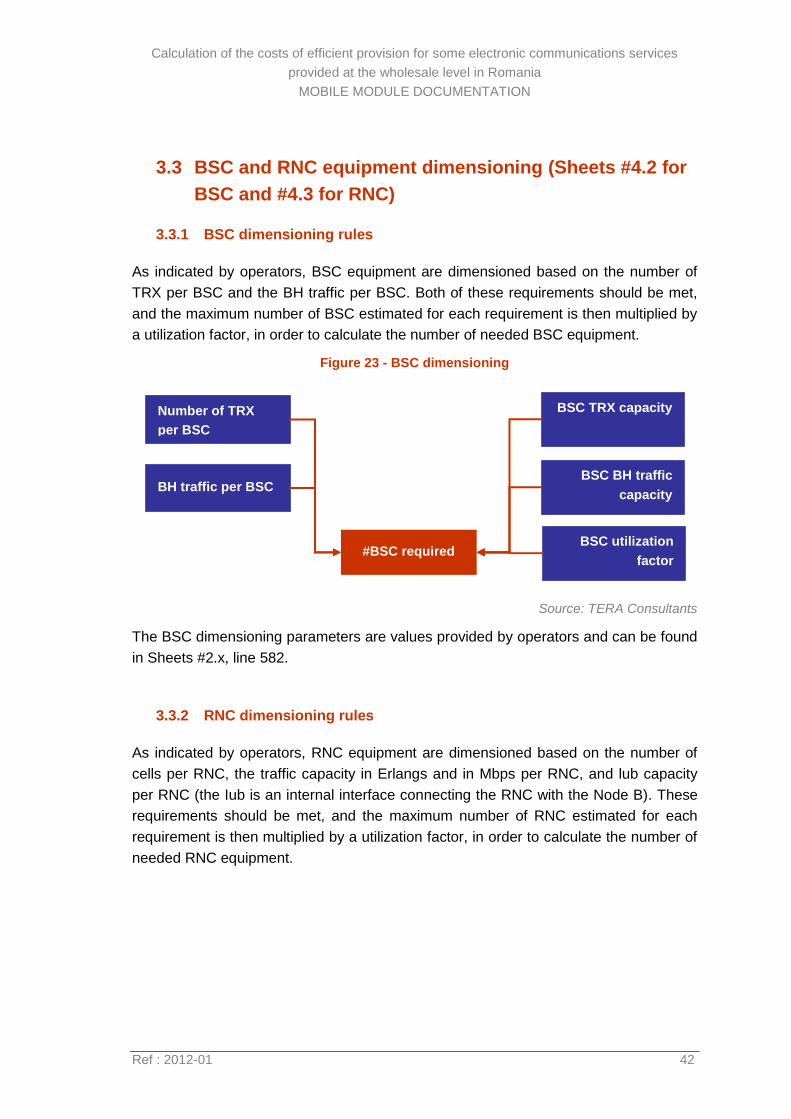
Calculation of the costs of efficient provision for some electronic communications services
provided at the wholesale level in Romania
MOBILE MODULE DOCUMENTATION
Ref : 2012-01 42
3.3 BSC and RNC equipment dimensioning (Sheets #4.2 for
BSC and #4.3 for RNC)
3.3.1 BSC dimensioning rules
As indicated by operators, BSC equipment are dimensioned based on the number of
TRX per BSC and the BH traffic per BSC. Both of these requirements should be met,
and the maximum number of BSC estimated for each requirement is then multiplied by
a utilization factor, in order to calculate the number of needed BSC equipment.
Figure 23 - BSC dimensioning
Source: TERA Consultants
The BSC dimensioning parameters are values provided by operators and can be found
in Sheets #2.x, line 582.
3.3.2 RNC dimensioning rules
As indicated by operators, RNC equipment are dimensioned based on the number of
cells per RNC, the traffic capacity in Erlangs and in Mbps per RNC, and lub capacity
per RNC (the Iub is an internal interface connecting the RNC with the Node B). These
requirements should be met, and the maximum number of RNC estimated for each
requirement is then multiplied by a utilization factor, in order to calculate the number of
needed RNC equipment.
BSC TRX capacity Number of TRX
per BSC
#BSC required
BH traffic per BSC BSC BH traffic
capacity
BSC utilization
factor
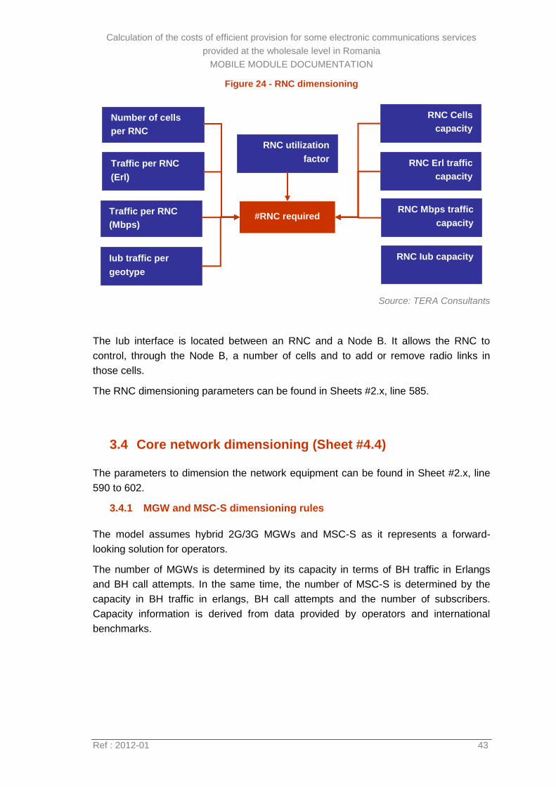
Calculation of the costs of efficient provision for some electronic communications services
provided at the wholesale level in Romania
MOBILE MODULE DOCUMENTATION
Ref : 2012-01 43
Figure 24 - RNC dimensioning
Source: TERA Consultants
The Iub interface is located between an RNC and a Node B. It allows the RNC to
control, through the Node B, a number of cells and to add or remove radio links in
those cells.
The RNC dimensioning parameters can be found in Sheets #2.x, line 585.
3.4 Core network dimensioning (Sheet #4.4)
The parameters to dimension the network equipment can be found in Sheet #2.x, line
590 to 602.
3.4.1 MGW and MSC-S dimensioning rules
The model assumes hybrid 2G/3G MGWs and MSC-S as it represents a forward-
looking solution for operators.
The number of MGWs is determined by its capacity in terms of BH traffic in Erlangs
and BH call attempts. In the same time, the number of MSC-S is determined by the
capacity in BH traffic in erlangs, BH call attempts and the number of subscribers.
Capacity information is derived from data provided by operators and international
benchmarks.
RNC Cells
capacity Number of cells
per RNC
#RNC required
Traffic per RNC
(Erl)
RNC Erl traffic
capacity
RNC Mbps traffic
capacity
Traffic per RNC
(Mbps)
RNC utilization
factor
Iub traffic per
geotype
RNC Iub capacity
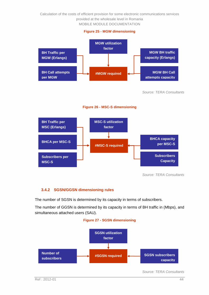
Calculation of the costs of efficient provision for some electronic communications services
provided at the wholesale level in Romania
MOBILE MODULE DOCUMENTATION
Ref : 2012-01 44
Figure 25 - MGW dimensioning
Source: TERA Consultants
Figure 26 - MSC-S dimensioning
Source: TERA Consultants
3.4.2 SGSN/GGSN dimensioning rules
The number of SGSN is determined by its capacity in terms of subscribers.
The number of GGSN is determined by its capacity in terms of BH traffic in (Mbps), and
simultaneous attached users (SAU).
Figure 27 - SGSN dimensioning
Source: TERA Consultants
Number of
subscribers #SGSN required
SGSN utilization
factor
SGSN subscribers
capacity
#MSC-S required
MSC-S utilization
factor
BHCA per MSC-S
Subscribers per
MSC-S
BHCA capacity
per MSC-S
Subscribers
Capacity
BH Traffic per
MSC (Erlangs)
MGW BH traffic
capacity (Erlangs)
BH Traffic per
MGW (Erlangs)
#MGW required
MGW utilization
factor
BH Call attempts
per MGW
MGW BH Call
attempts capacity
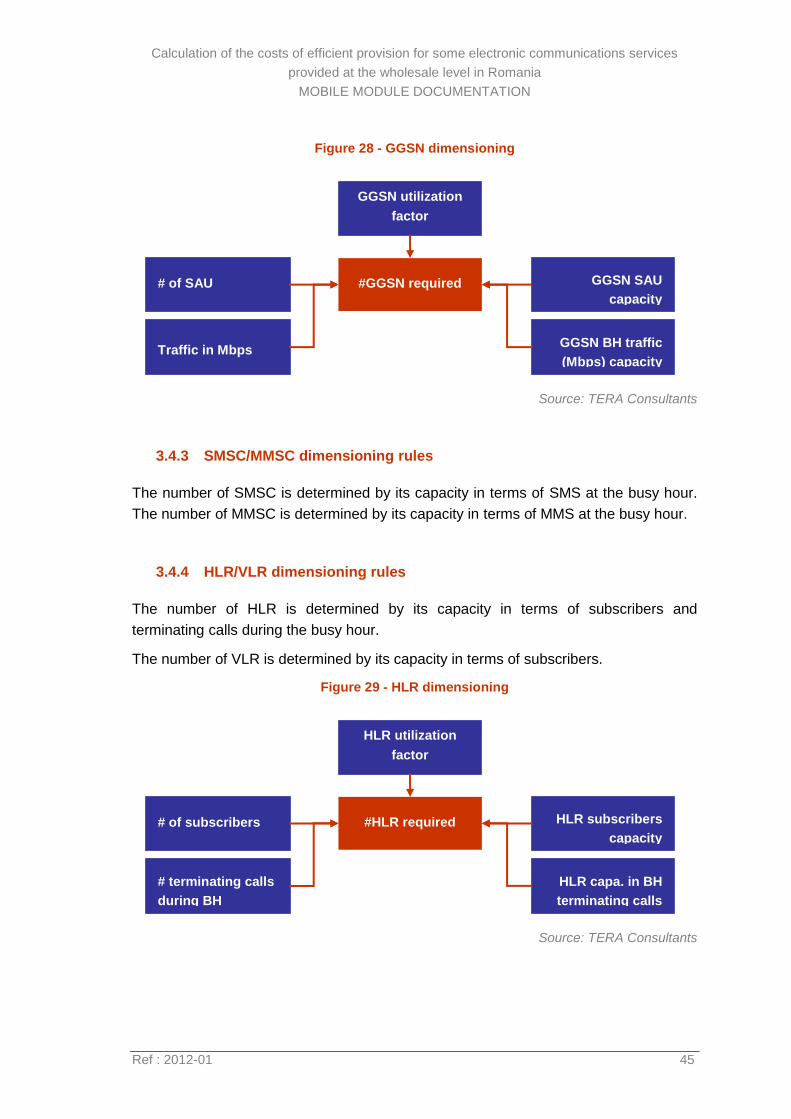
Calculation of the costs of efficient provision for some electronic communications services
provided at the wholesale level in Romania
MOBILE MODULE DOCUMENTATION
Ref : 2012-01 45
Figure 28 - GGSN dimensioning
Source: TERA Consultants
3.4.3 SMSC/MMSC dimensioning rules
The number of SMSC is determined by its capacity in terms of SMS at the busy hour.
The number of MMSC is determined by its capacity in terms of MMS at the busy hour.
3.4.4 HLR/VLR dimensioning rules
The number of HLR is determined by its capacity in terms of subscribers and
terminating calls during the busy hour.
The number of VLR is determined by its capacity in terms of subscribers.
Figure 29 - HLR dimensioning
Source: TERA Consultants
# of subscribers #HLR required
HLR utilization
factor
HLR subscribers
capacity
# terminating calls
during BH
HLR capa. in BH
terminating calls
# of SAU #GGSN required
GGSN utilization
factor
GGSN SAU
capacity
Traffic in Mbps GGSN BH traffic
(Mbps) capacity
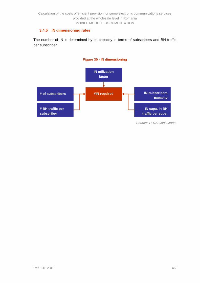
Calculation of the costs of efficient provision for some electronic communications services
provided at the wholesale level in Romania
MOBILE MODULE DOCUMENTATION
Ref : 2012-01 46
3.4.5 IN dimensioning rules
The number of IN is determined by its capacity in terms of subscribers and BH traffic
per subscriber.
Figure 30 - IN dimensioning
Source: TERA Consultants
# of subscribers #IN required
IN utilization
factor
IN subscribers
capacity
# BH traffic per
subscriber
IN capa. in BH
traffic per subs.
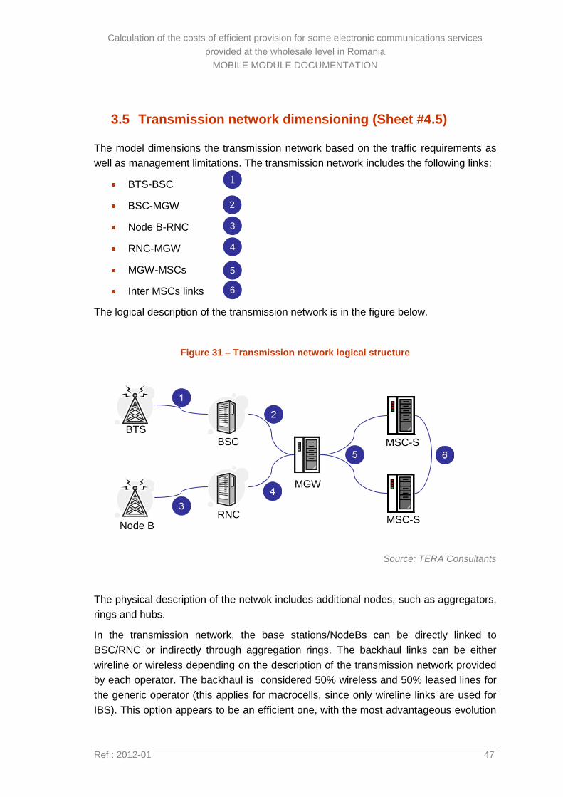
Calculation of the costs of efficient provision for some electronic communications services
provided at the wholesale level in Romania
MOBILE MODULE DOCUMENTATION
Ref : 2012-01 47
3.5 Transmission network dimensioning (Sheet #4.5)
The model dimensions the transmission network based on the traffic requirements as
well as management limitations. The transmission network includes the following links:
BTS-BSC
BSC-MGW
Node B-RNC
RNC-MGW
MGW-MSCs
Inter MSCs links
The logical description of the transmission network is in the figure below.
Figure 31 – Transmission network logical structure
Source: TERA Consultants
The physical description of the netwok includes additional nodes, such as aggregators,
rings and hubs.
In the transmission network, the base stations/NodeBs can be directly linked to
BSC/RNC or indirectly through aggregation rings. The backhaul links can be either
wireline or wireless depending on the description of the transmission network provided
by each operator. The backhaul is considered 50% wireless and 50% leased lines for
the generic operator (this applies for macrocells, since only wireline links are used for
IBS). This option appears to be an efficient one, with the most advantageous evolution
BTS
Node B
BSC
RNC
MGW
MSC-S
MSC-S
1
2
3
4
5
6
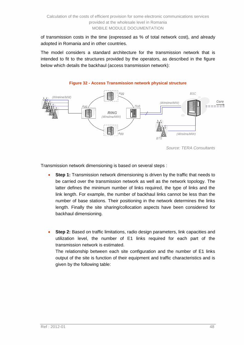
Calculation of the costs of efficient provision for some electronic communications services
provided at the wholesale level in Romania
MOBILE MODULE DOCUMENTATION
Ref : 2012-01 48
of transmission costs in the time (expressed as % of total network cost), and already
adopted in Romania and in other countries.
The model considers a standard architecture for the transmission network that is
intended to fit to the structures provided by the operators, as described in the figure
below which details the backhaul (access transmission network):
Figure 32 - Access Transmission network physical structure
Source: TERA Consultants
Transmission network dimensioning is based on several steps :
Step 1: Transmission network dimensioning is driven by the traffic that needs to
be carried over the transmission network as well as the network topology. The
latter defines the minimum number of links required, the type of links and the
link length. For example, the number of backhaul links cannot be less than the
number of base stations. Their positioning in the network determines the links
length. Finally the site sharing/collocation aspects have been considered for
backhaul dimensioning.
Step 2: Based on traffic limitations, radio design parameters, link capacities and
utilization level, the number of E1 links required for each part of the
transmission network is estimated.
The relationship between each site configuration and the number of E1 links
output of the site is function of their equipment and traffic characteristics and is
given by the following table:
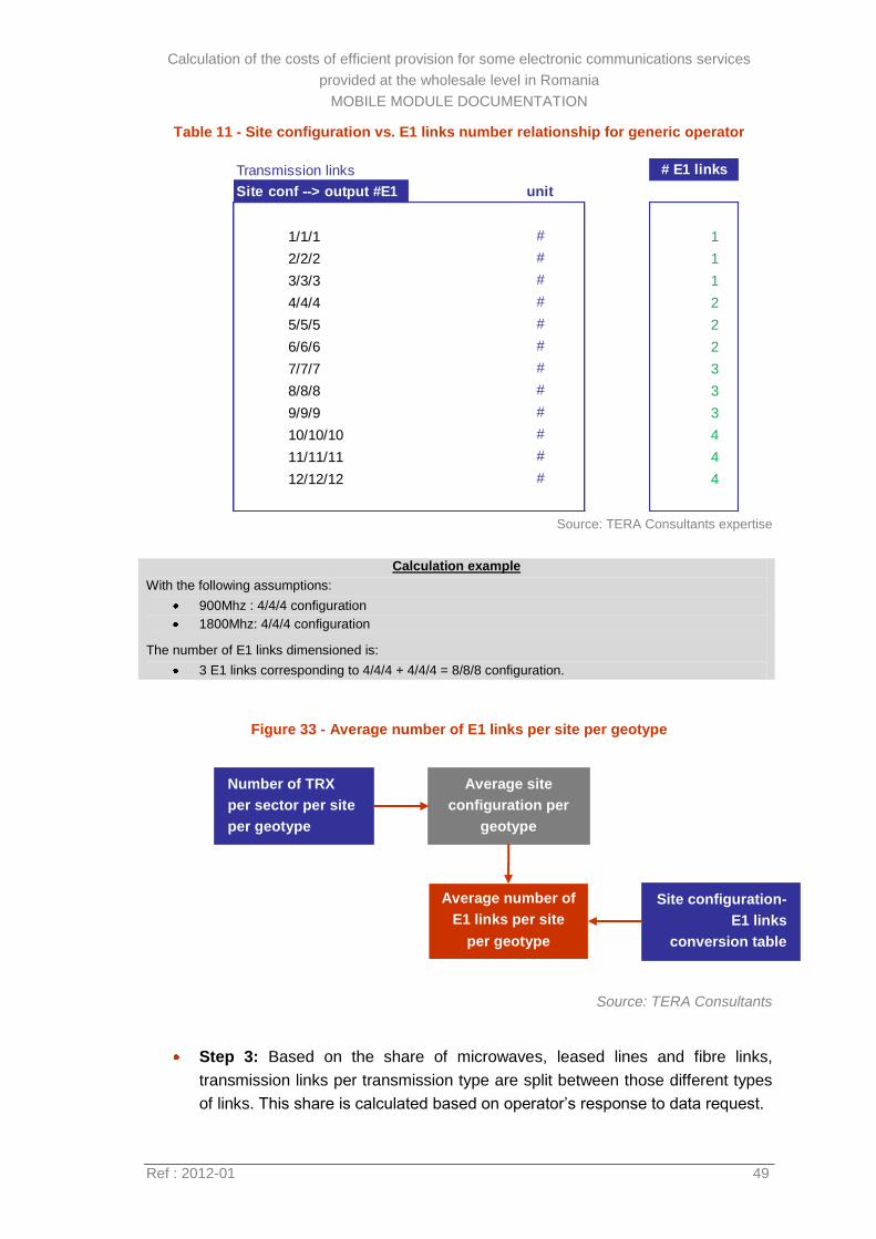
Calculation of the costs of efficient provision for some electronic communications services
provided at the wholesale level in Romania
MOBILE MODULE DOCUMENTATION
Ref : 2012-01 49
Table 11 - Site configuration vs. E1 links number relationship for generic operator
Source: TERA Consultants expertise
Calculation example
With the following assumptions:
900Mhz : 4/4/4 configuration
1800Mhz: 4/4/4 configuration
The number of E1 links dimensioned is:
3 E1 links corresponding to 4/4/4 + 4/4/4 = 8/8/8 configuration.
Figure 33 - Average number of E1 links per site per geotype
Source: TERA Consultants
Step 3: Based on the share of microwaves, leased lines and fibre links,
transmission links per transmission type are split between those different types
of links. This share is calculated based on operator’s response to data request.
Transmission links # E1 links
Site conf --> output #E1 unit
1/1/1 # 1
2/2/2 # 1
3/3/3 # 1
4/4/4 # 2
5/5/5 # 2
6/6/6 # 2
7/7/7 # 3
8/8/8 # 3
9/9/9 # 3
10/10/10 # 4
11/11/11 # 4
12/12/12 # 4
Site configuration-
E1 links
conversion table
Number of TRX
per sector per site
per geotype
Average number of
E1 links per site
per geotype
Average site
configuration per
geotype
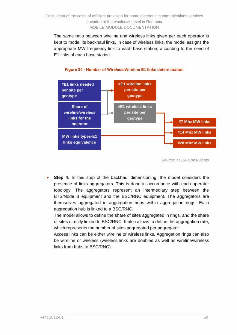
Calculation of the costs of efficient provision for some electronic communications services
provided at the wholesale level in Romania
MOBILE MODULE DOCUMENTATION
Ref : 2012-01 50
The same ratio between wireline and wireless links given per each operator is
kept to model its backhaul links. In case of wireless links, the model assigns the
appropriate MW frequency link to each base station, according to the need of
E1 links of each base station.
Figure 34 - Number of Wireless/Wireline E1 links determination
Source: TERA Consultants
Step 4: In this step of the backhaul dimensioning, the model considers the
presence of links aggregators. This is done in accordance with each operator
topology. The aggregators represent an intermediary step between the
BTS/Node B equipment and the BSC/RNC equipment. The aggregators are
themselves aggregated in aggregation hubs within aggregation rings. Each
aggregation hub is linked to a BSC/RNC.
The model allows to define the share of sites aggregated in rings, and the share
of sites directly linked to BSC/RNC. It also allows to define the aggregation rate,
which represents the number of sites aggregated per aggregator.
Access links can be either wireline or wireless links. Aggregation rings can also
be wireline or wireless (wireless links are doubled as well as wireline/wireless
links from hubs to BSC/RNC).
#E1 wireline links
per site per
geotype
#E1 links needed
per site per
geotype
#7 Mhz MW links
Share of
wireline/wireless
links for the
operator
#E1 wireless links
per site per
geotype
#14 Mhz MW links
#28 Mhz MW links
MW links types-E1
links equivalence
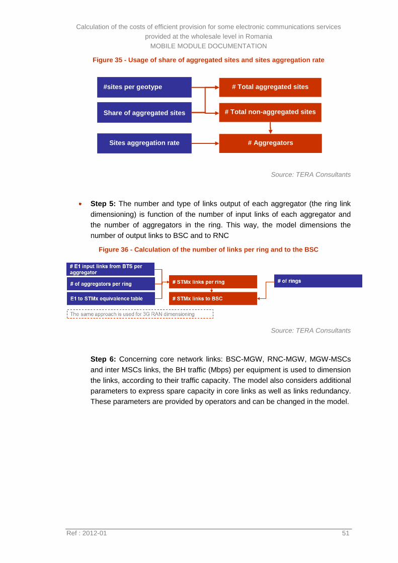
Calculation of the costs of efficient provision for some electronic communications services
provided at the wholesale level in Romania
MOBILE MODULE DOCUMENTATION
Ref : 2012-01 51
Figure 35 - Usage of share of aggregated sites and sites aggregation rate
Source: TERA Consultants
Step 5: The number and type of links output of each aggregator (the ring link
dimensioning) is function of the number of input links of each aggregator and
the number of aggregators in the ring. This way, the model dimensions the
number of output links to BSC and to RNC
Figure 36 - Calculation of the number of links per ring and to the BSC
Source: TERA Consultants
Step 6: Concerning core network links: BSC-MGW, RNC-MGW, MGW-MSCs
and inter MSCs links, the BH traffic (Mbps) per equipment is used to dimension
the links, according to their traffic capacity. The model also considers additional
parameters to express spare capacity in core links as well as links redundancy.
These parameters are provided by operators and can be changed in the model.
#sites per geotype
Share of aggregated sites
# Total aggregated sites
Sites aggregation rate
# Total non-aggregated sites
# Aggregators
Calculation of the costs of efficient provision for some electronic communications services
provided at the wholesale level in Romania
MOBILE MODULE DOCUMENTATION
Ref : 2012-01 52
4 Unit costs and OPEX
Once the model has calculated the required quantity of network elements, it calculates
the associated capital expenditures by applying modern equivalent asset (MEA) unit
costs. It then calculates the corresponding annuity by including the WACC, the price
trend and the economic lifetime, and it adds the OPEX.
4.1 Network element unit CAPEX (Sheet #5)
The asset unit CAPEX (i.e., prices paid for equipment added to cost of installation)
represents the evolution of MEA values. A full list of these CAPEX is contained in the
model and is displayed in the appendix 11.5. The unit CAPEX for each network
element for the generic operator was derived based on data received from the
operators and data incorporated in mobile LRIC models for other countries.
The model derives the final CAPEX unit cost estimates by taking, for each operator, the
provided value considering the price trend of equipment. These CAPEX inputs and
price trends are expressed in nominal terms and in Euros. The model is itself
expressed in Euros.
Network sites CAPEX is calculated for the sites owned in acquisition, or for the rented
sites considering administrative and development costs. The model assumes that all
the sites of the generic operator are rented (with administrative and development costs
to prepare the sites), and its costs are deduced from the costs observed for other
operators (usually an averaging method is applied). For collocated sites, especially for
core network collocated sites, the CAPEX per collocated element is calculated by
dividing the provided CAPEX of a collocated site by the number of collocated elements.
As for the transmission equipment unit costs, the values are derived from the data
submitted by operators (the values for the generic are obtained through an averaging
approach).
4.2 Network element OPEX
The principle of OPEX calculation in the model is based on the determination of
markups applied to CAPEX for each network component. This approach is standard
practice in bottom-up modelling.
The markup is obtained either provided by operator or issued from international
benchmark of practices, where operator figures were not available.
Calculation of the costs of efficient provision for some electronic communications services
provided at the wholesale level in Romania
MOBILE MODULE DOCUMENTATION
Ref : 2012-01 53
Sites OPEX include rental fees when sites are not owned in acquisition, and
maintenance fees12. This information is provided by operators. In accordance with
operators data, all the base station sites of the generic operator are owned in rental in
the perspective of an efficient operator. Moreover, the model assumes that 2G/3G sites
are collocated when possible, as well as 2G/3G IBS. For core equipment, the model
considers that BSC, RNC and MGW are collocated when possible, as well as other
core sites which are collocated in MGW and MSC-S. It is assumed that the generic
operator owns all the sites in rental (as for an efficient operator).
For microwave transmission equipment, OPEX used correspond to the values provided
by operator: aggregated OPEX or annual recurring fees.
The model also includes in network OPEX the spectrum fees (annual recurring fees),
that are considered as joint network costs applied to the RAN, and depending on the
number of carriers.
4.3 Total Network annual cost
Total annual costs are calculated by summing annual capital costs with operating and
maintenance costs.
12 The model assumes that the maintenance fees are already included in the CAPEX markup previously
defined, and hence put to zero in the model.
Calculation of the costs of efficient provision for some electronic communications services
provided at the wholesale level in Romania
MOBILE MODULE DOCUMENTATION
Ref : 2012-01 54
5 Additional costs (non-network costs)
In addition to previously calculated network costs, other cost items are considered for
LRAIC+ calculation. These costs are added in order to complete the perimeter of costs
to be allocated to network. The model includes the following costs:
Interconnection staff costs;
Licence costs;
subscribers acces costs;
Business overheads.
5.1 Interconnection specific costs
These specific costs are directly induced by interconnection service. They consist of
the cost of staff allocated specifically to interconnection.
As per the reference interconnection offers of the operators, some of the
interconnection specific costs are already recovered through the provision of ancillary
interconnection services, whose costs are being modeled in distinct a POI cost model.
Interconnection staff cost has been directly provided by operators.
Generic operator’s values correspond to the average of other operators’ responses.
To avoid double counting between interconnect specific costs and costs which are
recovered through the ancillary services, the model considers an input parameter of
50% that represents the share of interconnection staff cost allocated to regulated
termination. This parameter can be changed.
5.2 Licence costs
Spectrum license costs (one-off) are also included in the total costs for LRAIC+
calculation. They are considered as un-attributable common costs, recoverable from
the entire business. They are provided by ANCOM and consist of the initial license fee
valued based on the results of a recent licence auction in Romania.
It is assumed for the generic operator a spectrum allocation resulting of an auction.
Considering the bandwidths, it is made the following assumptions:
900 Mhz: 10 Mhz,
1800 Mhz: 10 Mhz
2100 Mhz: 15 Mhz,
Calculation of the costs of efficient provision for some electronic communications services
provided at the wholesale level in Romania
MOBILE MODULE DOCUMENTATION
Ref : 2012-01 55
considering this to be representative for a generic mobile operator acting on the
Romanian market. The parameters to define the spectrum allocation can be found in
Sheet #2.x, line 368 to 384.
These spectrum assumptions are valued according to ANCOM at 160 M€ for the
generic operator (133 M€ for 2G and 27 M€ for 3G).
These costs13 are allocated as business overheads. The model applies a markup to the
network costs (calculated as percentage of licence fee total costs in the sum of network
costs and retail costs) resulting in licence fees unit costs.
5.3 Subscriber access
Alongside the calculation of unit traffic termination cost, the model calculates an
additional per subscriber cost based on SIM cards evolution. The cost of SIM Cards is
benchmarked from international models, and depreciated on its economic life14. The
resulting unit cost per subscriber is not applicable on unit traffic (minute, sms or MB)
but equals to a cost per subscriber per month. It is calculated for 2G and 3G SIM cards.
On top of the cost of SIM cards, the model provides the possibility to allocate network
equipment costs that are subscriber-driven to a subscriber access cost. The allocation
keys are based either on a proportionality rule (subscriber-driven vs. traffic-driven) or
on a EPMU rule.
5.4 Business overheads
The business overheads are considered in the model as a markup applied to the total
of the network costs. The business overheads to be taken into account must be only
those relevant to network. The model defines a markup to derive the network
component of business overheads from the total network cost.
This markup is obtained from the three following parameters provided by operators15:
Network costs;
Retail costs;
Un-attributable costs.
The markup represents the percentage of un-attributable costs in the sum of network
costs and retail costs and is applied to the network unit cost.
The model assumes that generic operator business overheads correspond to the
average business overheads of four operators.
13 Source: ANCOM
14 4 years, issued from benchmark
15 Total costs of operators consist of the provided information contained in the operators’ accounts :
network costs, un-attributable costs, and retail costs
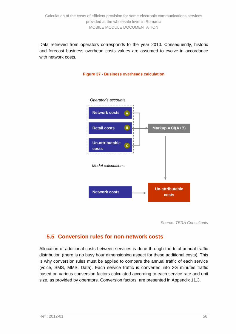
Calculation of the costs of efficient provision for some electronic communications services
provided at the wholesale level in Romania
MOBILE MODULE DOCUMENTATION
Ref : 2012-01 56
Data retrieved from operators corresponds to the year 2010. Consequently, historic
and forecast business overhead costs values are assumed to evolve in accordance
with network costs.
Figure 37 - Business overheads calculation
Source: TERA Consultants
5.5 Conversion rules for non-network costs
Allocation of additional costs between services is done through the total annual traffic
distribution (there is no busy hour dimensioning aspect for these additional costs). This
is why conversion rules must be applied to compare the annual traffic of each service
(voice, SMS, MMS, Data). Each service traffic is converted into 2G minutes traffic
based on various conversion factors calculated according to each service rate and unit
size, as provided by operators. Conversion factors are presented in Appendix 11.3.
Network costs
Retail costs
Un-attributable
costs
Operator’s accounts
Model calculations
Network costs
Markup = C/(A+B)
Un-attributable
costs
Calculation of the costs of efficient provision for some electronic communications services
provided at the wholesale level in Romania
MOBILE MODULE DOCUMENTATION
Ref : 2012-01 57
6 Depreciation
There is a very large number of approaches to depreciate an investment, but NRAs in
Europe mainly use economic depreciation when implementing bottom-up model rather
than accounting depreciation with straight line annuities.
Economic depreciation calculates annuities that evolve with expected incomes
generated by the asset over the asset’s useful life. Economic depreciation is defined
simply as the period-by-period change in the market value of an asset. The market
value of an asset is equal to the present value of the income that the asset is expected
to generate over the remainder of its useful life.
The model calculates the economic depreciation for all services (LRAIC+) and for the
sole increment (Pure LRIC) in Sheets #8.1 to 8.4.
The aim of this approach is to calculate the yearly incremental cost of the whole
network, during the period 2006 – 203016.
The first step is to determine the incremental quantity of equipment, sites, and
transmission links each year. This calculation is based on the network
dimensioning results obtained in the previous paragraphs, and takes into
account the economic life of equipment to determine the number of equipment
renewed each year.
Once the incremental number of network equipment, sites and transmission
links is known, the next step is to deduce the corresponding incremental
network cost, multiplying the incremental number of units by the unit CAPEX
and unit OPEX.
The quantity of usage of each equipment is determined for each service. These
values have been previously calculated for LRAIC cost (Cf. section 7.1.1).
Values after 2020 are maintained until 203017.
The total network cost (total cost for each network equipment) is then allocated
to the services in order to determine a constant economic cost for each service.
16 Extension of 2006-2020 period to 2030 allows to englobe all the equipment with their economic lives for
the economic depreciation calculation. After 2020 the traffic is maintained as is until 2030.
17 As the model considers that additional traffic represents the traffic corresponding to 4G (LTE)
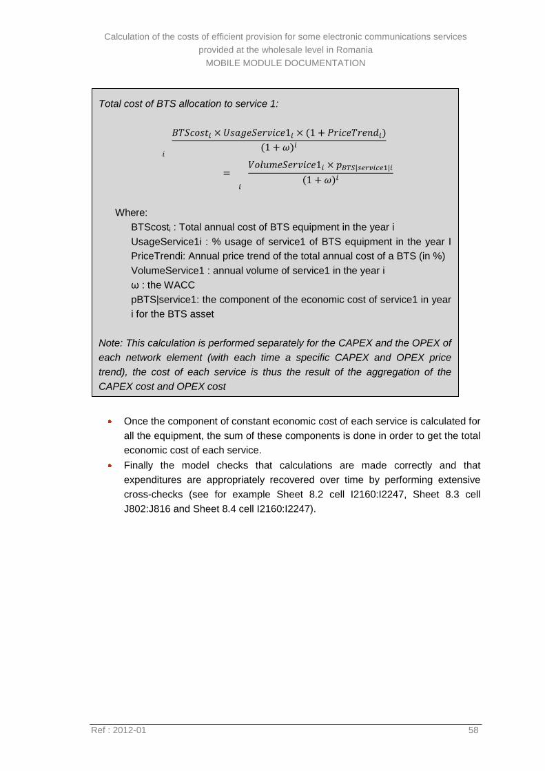
Calculation of the costs of efficient provision for some electronic communications services
provided at the wholesale level in Romania
MOBILE MODULE DOCUMENTATION
Ref : 2012-01 58
Once the component of constant economic cost of each service is calculated for
all the equipment, the sum of these components is done in order to get the total
economic cost of each service.
Finally the model checks that calculations are made correctly and that
expenditures are appropriately recovered over time by performing extensive
cross-checks (see for example Sheet 8.2 cell I2160:I2247, Sheet 8.3 cell
J802:J816 and Sheet 8.4 cell I2160:I2247).
Total cost of BTS allocation to service 1:
Where:
BTScosti : Total annual cost of BTS equipment in the year i
UsageService1i : % usage of service1 of BTS equipment in the year I
PriceTrendi: Annual price trend of the total annual cost of a BTS (in %)
VolumeService1 : annual volume of service1 in the year i
ω : the WACC
pBTS|service1: the component of the economic cost of service1 in year
i for the BTS asset
Note: This calculation is performed separately for the CAPEX and the OPEX of
each network element (with each time a specific CAPEX and OPEX price
trend), the cost of each service is thus the result of the aggregation of the
CAPEX cost and OPEX cost
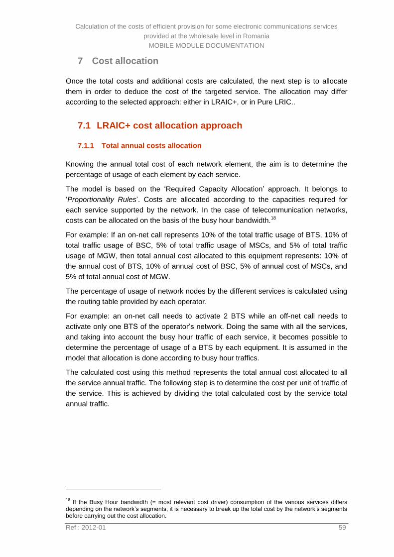
Calculation of the costs of efficient provision for some electronic communications services
provided at the wholesale level in Romania
MOBILE MODULE DOCUMENTATION
Ref : 2012-01 59
7 Cost allocation
Once the total costs and additional costs are calculated, the next step is to allocate
them in order to deduce the cost of the targeted service. The allocation may differ
according to the selected approach: either in LRAIC+, or in Pure LRIC..
7.1 LRAIC+ cost allocation approach
7.1.1 Total annual costs allocation
Knowing the annual total cost of each network element, the aim is to determine the
percentage of usage of each element by each service.
The model is based on the ‘Required Capacity Allocation’ approach. It belongs to
‘Proportionality Rules’. Costs are allocated according to the capacities required for
each service supported by the network. In the case of telecommunication networks,
costs can be allocated on the basis of the busy hour bandwidth.18
For example: If an on-net call represents 10% of the total traffic usage of BTS, 10% of
total traffic usage of BSC, 5% of total traffic usage of MSCs, and 5% of total traffic
usage of MGW, then total annual cost allocated to this equipment represents: 10% of
the annual cost of BTS, 10% of annual cost of BSC, 5% of annual cost of MSCs, and
5% of total annual cost of MGW.
The percentage of usage of network nodes by the different services is calculated using
the routing table provided by each operator.
For example: an on-net call needs to activate 2 BTS while an off-net call needs to
activate only one BTS of the operator’s network. Doing the same with all the services,
and taking into account the busy hour traffic of each service, it becomes possible to
determine the percentage of usage of a BTS by each equipment. It is assumed in the
model that allocation is done according to busy hour traffics.
The calculated cost using this method represents the total annual cost allocated to all
the service annual traffic. The following step is to determine the cost per unit of traffic of
the service. This is achieved by dividing the total calculated cost by the service total
annual traffic.
18 If the Busy Hour bandwidth (= most relevant cost driver) consumption of the various services differs
depending on the network’s segments, it is necessary to break up the total cost by the network’s segments before carrying out the cost allocation.
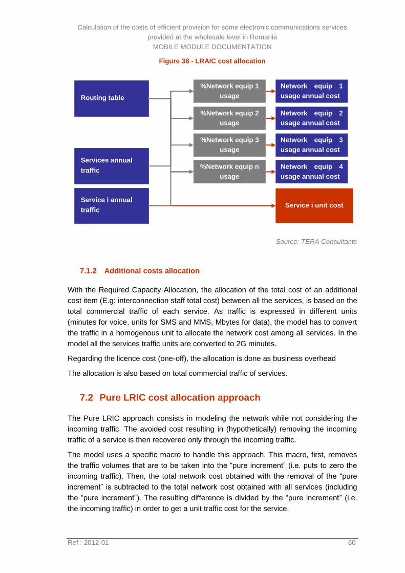
Calculation of the costs of efficient provision for some electronic communications services
provided at the wholesale level in Romania
MOBILE MODULE DOCUMENTATION
Ref : 2012-01 60
Figure 38 - LRAIC cost allocation
Source: TERA Consultants
7.1.2 Additional costs allocation
With the Required Capacity Allocation, the allocation of the total cost of an additional
cost item (E.g: interconnection staff total cost) between all the services, is based on the
total commercial traffic of each service. As traffic is expressed in different units
(minutes for voice, units for SMS and MMS, Mbytes for data), the model has to convert
the traffic in a homogenous unit to allocate the network cost among all services. In the
model all the services traffic units are converted to 2G minutes.
Regarding the licence cost (one-off), the allocation is done as business overhead
The allocation is also based on total commercial traffic of services.
7.2 Pure LRIC cost allocation approach
The Pure LRIC approach consists in modeling the network while not considering the
incoming traffic. The avoided cost resulting in (hypothetically) removing the incoming
traffic of a service is then recovered only through the incoming traffic.
The model uses a specific macro to handle this approach. This macro, first, removes
the traffic volumes that are to be taken into the “pure increment” (i.e. puts to zero the
incoming traffic). Then, the total network cost obtained with the removal of the “pure
increment” is subtracted to the total network cost obtained with all services (including
the “pure increment”). The resulting difference is divided by the “pure increment” (i.e.
the incoming traffic) in order to get a unit traffic cost for the service.
Routing table
%Network equip 1
usage
Service i unit cost
%Network equip 2
usage
%Network equip 3
usage
%Network equip n
usage
Network equip 1
usage annual cost
Network equip 2
usage annual cost
Network equip 3
usage annual cost
Network equip 4
usage annual cost
Service i annual
traffic
Services annual
traffic
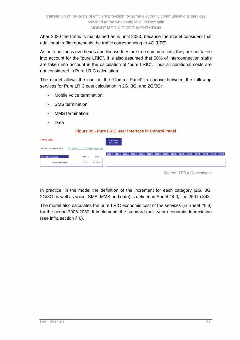
Calculation of the costs of efficient provision for some electronic communications services
provided at the wholesale level in Romania
MOBILE MODULE DOCUMENTATION
Ref : 2012-01 61
After 2020 the traffic is maintained as is until 2030, because the model considers that
additional traffic represents the traffic corresponding to 4G (LTE).
As both business overheads and license fees are true common cots, they are not taken
into account for the “pure LRIC”. It is also assumed that 50% of interconnection staffs
are taken into account in the calculation of “pure LRIC”. Thus all additional costs are
not considered in Pure LRIC calculation.
The model allows the user in the ‘Control Panel’ to choose between the following
services for Pure LRIC cost calculation in 2G, 3G, and 2G/3G:
Mobile voice termination;
SMS termination;
MMS termination;
Data
Figure 39 - Pure LRIC user interface in Control Panel
Source: TERA Consultants
In practice, in the model the definition of the increment for each category (2G, 3G,
2G/3G as well as voice, SMS, MMS and data) is defined in Sheet #4.0, line 260 to 343.
The model also calculates the pure LRIC economic cost of the services (in Sheet #8.3)
for the period 2006-2030. It implements the standard multi-year economic depreciation
(see infra section § 6).
PURE LRIC
Service cost in Pure LRIC 2G/3G Mobile Termination
2006 A 2007 A 2008 A 2009 A 2010 A 2011 E 2012 E 2013 E 2014 E 2015 E 2016 E 2017 E 2018 E 2019 E 2020 E
Pure LRIC unit cost label 1 unit
Mobile Termination 2G/3G EUR/unit
Calculate Pure LRIC
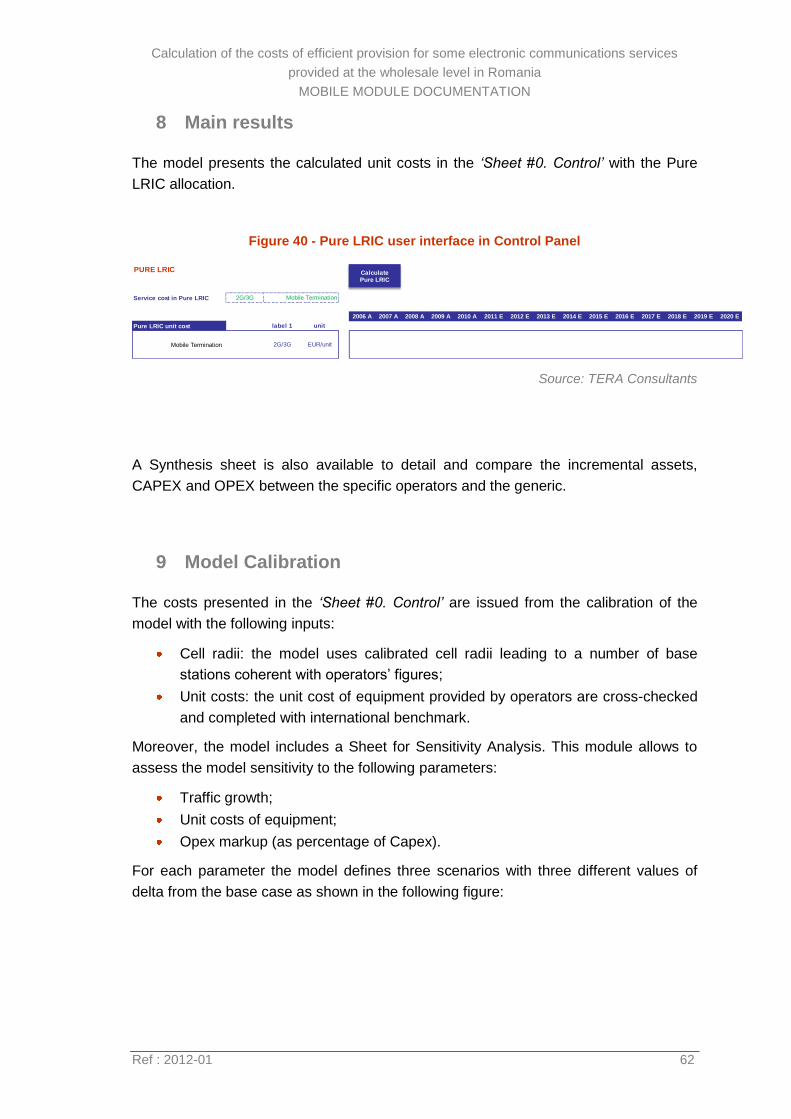
Calculation of the costs of efficient provision for some electronic communications services
provided at the wholesale level in Romania
MOBILE MODULE DOCUMENTATION
Ref : 2012-01 62
8 Main results
The model presents the calculated unit costs in the ‘Sheet #0. Control’ with the Pure
LRIC allocation.
Figure 40 - Pure LRIC user interface in Control Panel
Source: TERA Consultants
A Synthesis sheet is also available to detail and compare the incremental assets,
CAPEX and OPEX between the specific operators and the generic.
9 Model Calibration
The costs presented in the ‘Sheet #0. Control’ are issued from the calibration of the
model with the following inputs:
Cell radii: the model uses calibrated cell radii leading to a number of base
stations coherent with operators’ figures;
Unit costs: the unit cost of equipment provided by operators are cross-checked
and completed with international benchmark.
Moreover, the model includes a Sheet for Sensitivity Analysis. This module allows to
assess the model sensitivity to the following parameters:
Traffic growth;
Unit costs of equipment;
Opex markup (as percentage of Capex).
For each parameter the model defines three scenarios with three different values of
delta from the base case as shown in the following figure:
PURE LRIC
Service cost in Pure LRIC 2G/3G Mobile Termination
2006 A 2007 A 2008 A 2009 A 2010 A 2011 E 2012 E 2013 E 2014 E 2015 E 2016 E 2017 E 2018 E 2019 E 2020 E
Pure LRIC unit cost label 1 unit
Mobile Termination 2G/3G EUR/unit
Calculate Pure LRIC
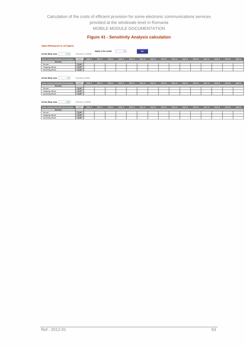
Calculation of the costs of efficient provision for some electronic communications services
provided at the wholesale level in Romania
MOBILE MODULE DOCUMENTATION
Ref : 2012-01 63
Figure 41 - Sensitivity Analysis calculation
Opex Markup (as % of Capex)
Apply in the model 0%
Δ from Base case -20% Scenario 1 (-20%)
Unit 2006 A 2007 A 2008 A 2009 A 2010 A 2011 E 2012 E 2013 E 2014 E 2015 E 2016 E 2017 E 2018 E 2019 E 2020 E
On-net EUR
Outgoing off-net EUR
Incoming off-net EUR
Δ from Base case 0% Scenario 2 (0%)
Unit 2006 A 2007 A 2008 A 2009 A 2010 A 2011 E 2012 E 2013 E 2014 E 2015 E 2016 E 2017 E 2018 E 2019 E 2020 E
On-net EUR
Outgoing off-net EUR
Incoming off-net EUR
Δ from Base case 20% Scenario 3 (20%)
Unit 2006 A 2007 A 2008 A 2009 A 2010 A 2011 E 2012 E 2013 E 2014 E 2015 E 2016 E 2017 E 2018 E 2019 E 2020 E
On-net EUR
Outgoing off-net EUR
Incoming off-net EUR
Service
Voice services blended termination
Service
Voice services blended termination
Service
Voice services blended termination
Go
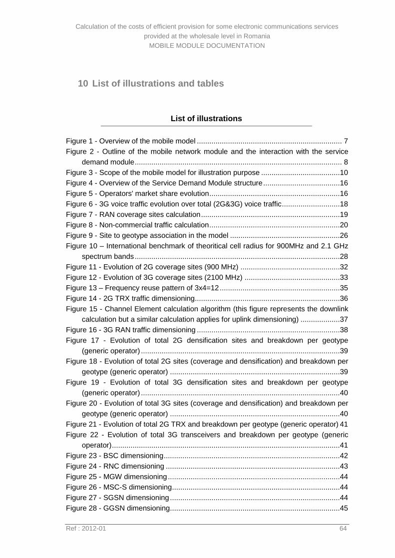
Calculation of the costs of efficient provision for some electronic communications services
provided at the wholesale level in Romania
MOBILE MODULE DOCUMENTATION
Ref : 2012-01 64
10 List of illustrations and tables
List of illustrations
Figure 1 - Overview of the mobile model ...................................................................... 7
Figure 2 - Outline of the mobile network module and the interaction with the service
demand module .................................................................................................... 8
Figure 3 - Scope of the mobile model for illustration purpose ......................................10
Figure 4 - Overview of the Service Demand Module structure .....................................16
Figure 5 - Operators' market share evolution ...............................................................16
Figure 6 - 3G voice traffic evolution over total (2G&3G) voice traffic ............................18
Figure 7 - RAN coverage sites calculation ...................................................................19
Figure 8 - Non-commercial traffic calculation ...............................................................20
Figure 9 - Site to geotype association in the model .....................................................26
Figure 10 – International benchmark of theoritical cell radius for 900MHz and 2.1 GHz
spectrum bands ...................................................................................................28
Figure 11 - Evolution of 2G coverage sites (900 MHz) ................................................32
Figure 12 - Evolution of 3G coverage sites (2100 MHz) ..............................................33
Figure 13 – Frequency reuse pattern of 3x4=12 ..........................................................35
Figure 14 - 2G TRX traffic dimensioning ......................................................................36
Figure 15 - Channel Element calculation algorithm (this figure represents the downlink
calculation but a similar calculation applies for uplink dimensioning) ...................37
Figure 16 - 3G RAN traffic dimensioning .....................................................................38
Figure 17 - Evolution of total 2G densification sites and breakdown per geotype
(generic operator) ................................................................................................39
Figure 18 - Evolution of total 2G sites (coverage and densification) and breakdown per
geotype (generic operator) ..................................................................................39
Figure 19 - Evolution of total 3G densification sites and breakdown per geotype
(generic operator) ................................................................................................40
Figure 20 - Evolution of total 3G sites (coverage and densification) and breakdown per
geotype (generic operator) ..................................................................................40
Figure 21 - Evolution of total 2G TRX and breakdown per geotype (generic operator) 41
Figure 22 - Evolution of total 3G transceivers and breakdown per geotype (generic
operator) ..............................................................................................................41
Figure 23 - BSC dimensioning .....................................................................................42
Figure 24 - RNC dimensioning ....................................................................................43
Figure 25 - MGW dimensioning ...................................................................................44
Figure 26 - MSC-S dimensioning .................................................................................44
Figure 27 - SGSN dimensioning ..................................................................................44
Figure 28 - GGSN dimensioning..................................................................................45
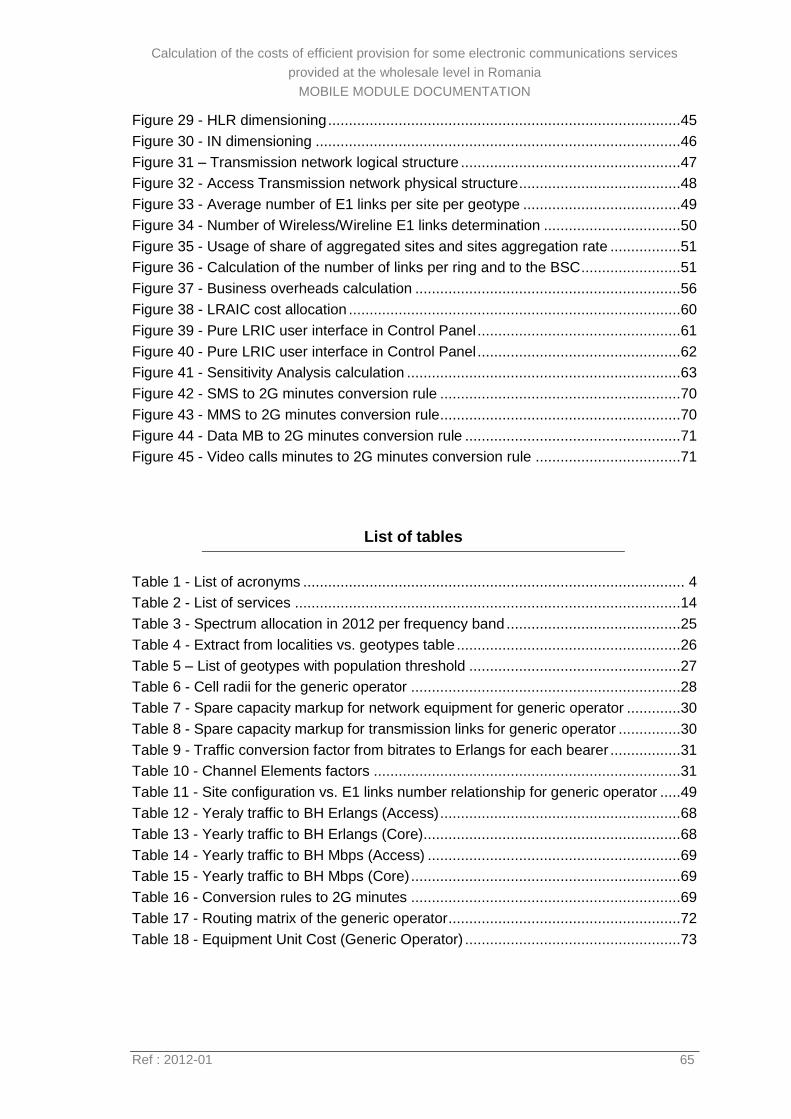
Calculation of the costs of efficient provision for some electronic communications services
provided at the wholesale level in Romania
MOBILE MODULE DOCUMENTATION
Ref : 2012-01 65
Figure 29 - HLR dimensioning .....................................................................................45
Figure 30 - IN dimensioning ........................................................................................46
Figure 31 – Transmission network logical structure .....................................................47
Figure 32 - Access Transmission network physical structure .......................................48
Figure 33 - Average number of E1 links per site per geotype ......................................49
Figure 34 - Number of Wireless/Wireline E1 links determination .................................50
Figure 35 - Usage of share of aggregated sites and sites aggregation rate .................51
Figure 36 - Calculation of the number of links per ring and to the BSC ........................51
Figure 37 - Business overheads calculation ................................................................56
Figure 38 - LRAIC cost allocation ................................................................................60
Figure 39 - Pure LRIC user interface in Control Panel .................................................61
Figure 40 - Pure LRIC user interface in Control Panel .................................................62
Figure 41 - Sensitivity Analysis calculation ..................................................................63
Figure 42 - SMS to 2G minutes conversion rule ..........................................................70
Figure 43 - MMS to 2G minutes conversion rule ..........................................................70
Figure 44 - Data MB to 2G minutes conversion rule ....................................................71
Figure 45 - Video calls minutes to 2G minutes conversion rule ...................................71
List of tables
Table 1 - List of acronyms ............................................................................................ 4
Table 2 - List of services .............................................................................................14
Table 3 - Spectrum allocation in 2012 per frequency band ..........................................25
Table 4 - Extract from localities vs. geotypes table ......................................................26
Table 5 – List of geotypes with population threshold ...................................................27
Table 6 - Cell radii for the generic operator .................................................................28
Table 7 - Spare capacity markup for network equipment for generic operator .............30
Table 8 - Spare capacity markup for transmission links for generic operator ...............30
Table 9 - Traffic conversion factor from bitrates to Erlangs for each bearer .................31
Table 10 - Channel Elements factors ..........................................................................31
Table 11 - Site configuration vs. E1 links number relationship for generic operator .....49
Table 12 - Yeraly traffic to BH Erlangs (Access) ..........................................................68
Table 13 - Yearly traffic to BH Erlangs (Core) ..............................................................68
Table 14 - Yearly traffic to BH Mbps (Access) .............................................................69
Table 15 - Yearly traffic to BH Mbps (Core) .................................................................69
Table 16 - Conversion rules to 2G minutes .................................................................69
Table 17 - Routing matrix of the generic operator ........................................................72
Table 18 - Equipment Unit Cost (Generic Operator) ....................................................73
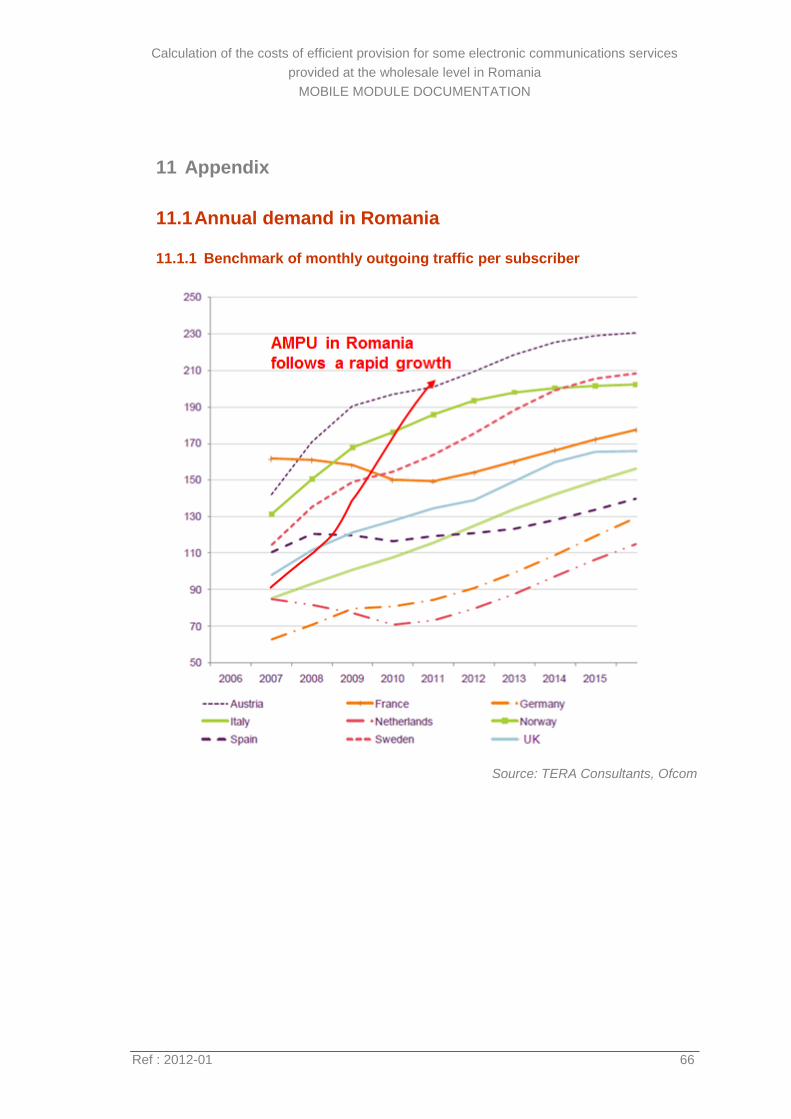
Calculation of the costs of efficient provision for some electronic communications services
provided at the wholesale level in Romania
MOBILE MODULE DOCUMENTATION
Ref : 2012-01 66
11 Appendix
11.1 Annual demand in Romania
11.1.1 Benchmark of monthly outgoing traffic per subscriber
Source: TERA Consultants, Ofcom
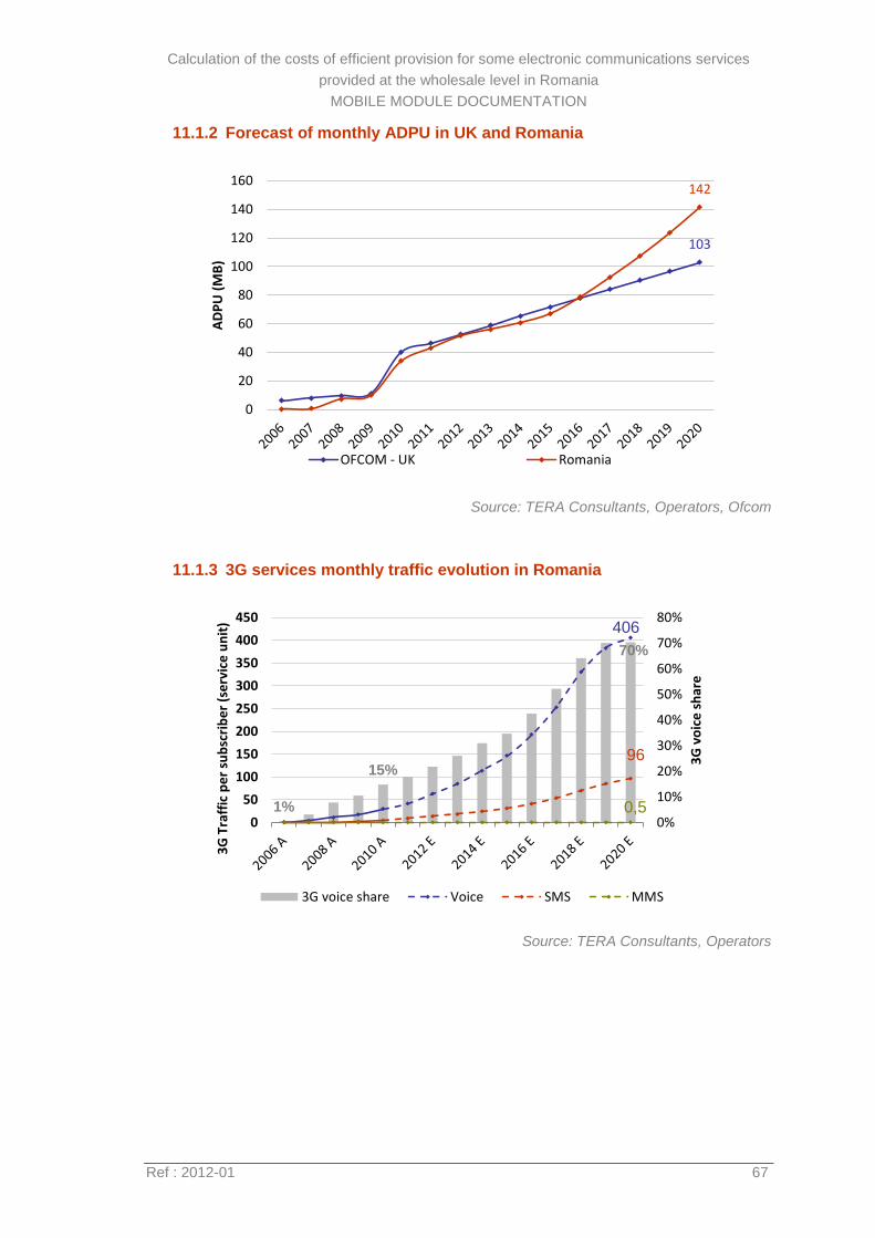
Calculation of the costs of efficient provision for some electronic communications services
provided at the wholesale level in Romania
MOBILE MODULE DOCUMENTATION
Ref : 2012-01 67
11.1.2 Forecast of monthly ADPU in UK and Romania
Source: TERA Consultants, Operators, Ofcom
11.1.3 3G services monthly traffic evolution in Romania
Source: TERA Consultants, Operators
103
142
0
20
40
60
80
100
120
140
160
AD
PU
(M
B)
OFCOM - UK Romania
1%
15%
70%
0%
10%
20%
30%
40%
50%
60%
70%
80%
0
50
100
150
200
250
300
350
400
450
3G
vo
ice
sh
are
3G
Tra
ffic
pe
r su
bsc
rib
er
(se
rvic
e u
nit
)
3G voice share Voice SMS MMS
96
406
0,5
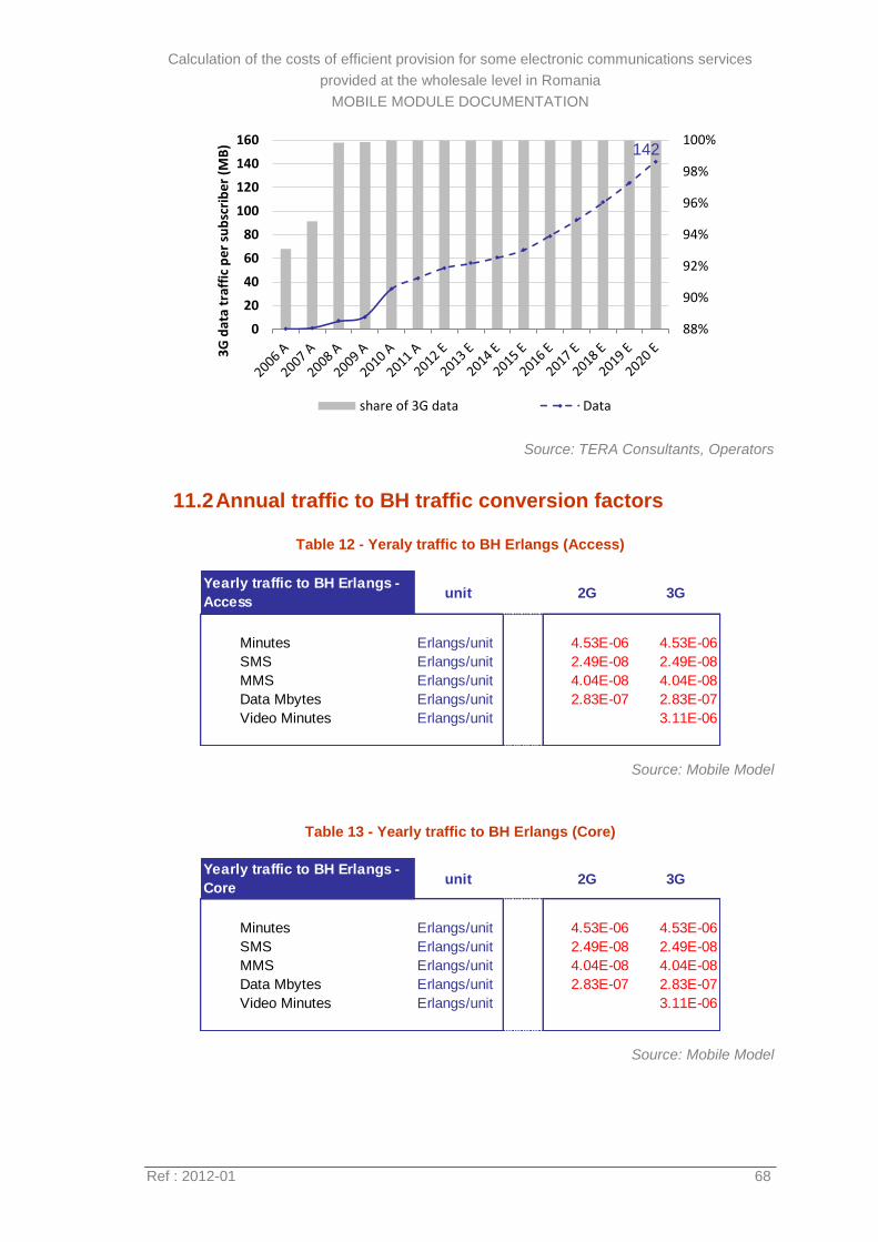
Calculation of the costs of efficient provision for some electronic communications services
provided at the wholesale level in Romania
MOBILE MODULE DOCUMENTATION
Ref : 2012-01 68
Source: TERA Consultants, Operators
11.2 Annual traffic to BH traffic conversion factors
Table 12 - Yeraly traffic to BH Erlangs (Access)
Source: Mobile Model
Table 13 - Yearly traffic to BH Erlangs (Core)
Source: Mobile Model
88%
90%
92%
94%
96%
98%
100%
0
20
40
60
80
100
120
140
160
3G
dat
a tr
affi
c p
er
sub
scri
be
r (M
B)
share of 3G data Data
142
unit 2G 3G
Minutes Erlangs/unit 4.53E-06 4.53E-06
SMS Erlangs/unit 2.49E-08 2.49E-08
MMS Erlangs/unit 4.04E-08 4.04E-08
Data Mbytes Erlangs/unit 2.83E-07 2.83E-07
Video Minutes Erlangs/unit 3.11E-06
Yearly traffic to BH Erlangs -
Access
unit 2G 3G
Minutes Erlangs/unit 4.53E-06 4.53E-06
SMS Erlangs/unit 2.49E-08 2.49E-08
MMS Erlangs/unit 4.04E-08 4.04E-08
Data Mbytes Erlangs/unit 2.83E-07 2.83E-07
Video Minutes Erlangs/unit 3.11E-06
Yearly traffic to BH Erlangs -
Core
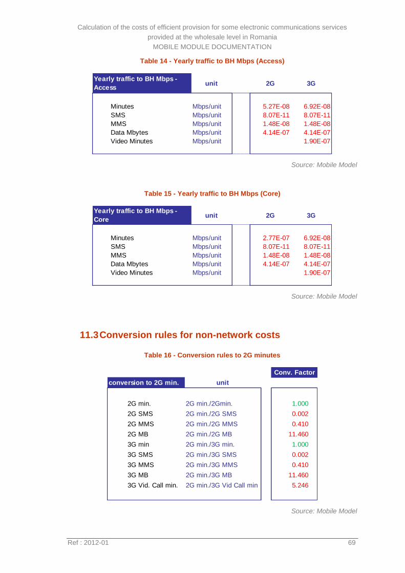
Calculation of the costs of efficient provision for some electronic communications services
provided at the wholesale level in Romania
MOBILE MODULE DOCUMENTATION
Ref : 2012-01 69
Table 14 - Yearly traffic to BH Mbps (Access)
Source: Mobile Model
Table 15 - Yearly traffic to BH Mbps (Core)
Source: Mobile Model
11.3 Conversion rules for non-network costs
Table 16 - Conversion rules to 2G minutes
Source: Mobile Model
unit 2G 3G
Minutes Mbps/unit 5.27E-08 6.92E-08
SMS Mbps/unit 8.07E-11 8.07E-11
MMS Mbps/unit 1.48E-08 1.48E-08
Data Mbytes Mbps/unit 4.14E-07 4.14E-07
Video Minutes Mbps/unit 1.90E-07
Yearly traffic to BH Mbps -
Access
unit 2G 3G
Minutes Mbps/unit 2.77E-07 6.92E-08
SMS Mbps/unit 8.07E-11 8.07E-11
MMS Mbps/unit 1.48E-08 1.48E-08
Data Mbytes Mbps/unit 4.14E-07 4.14E-07
Video Minutes Mbps/unit 1.90E-07
Yearly traffic to BH Mbps -
Core
Conv. Factor
unit
2G min. 2G min./2Gmin. 1.000
2G SMS 2G min./2G SMS 0.002
2G MMS 2G min./2G MMS 0.410
2G MB 2G min./2G MB 11.460
3G min 2G min./3G min. 1.000
3G SMS 2G min./3G SMS 0.002
3G MMS 2G min./3G MMS 0.410
3G MB 2G min./3G MB 11.460
3G Vid. Call min. 2G min./3G Vid Call min 5.246
conversion to 2G min.
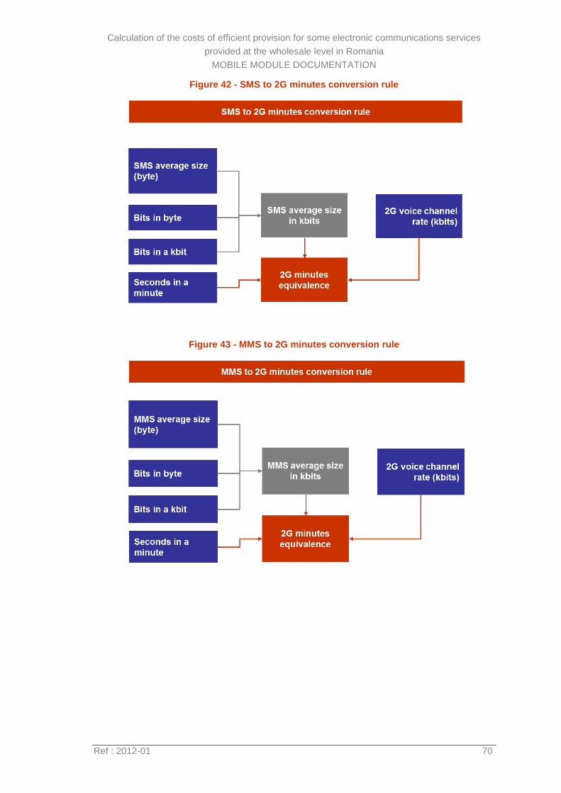
Calculation of the costs of efficient provision for some electronic communications services
provided at the wholesale level in Romania
MOBILE MODULE DOCUMENTATION
Ref : 2012-01 70
Figure 42 - SMS to 2G minutes conversion rule
Figure 43 - MMS to 2G minutes conversion rule
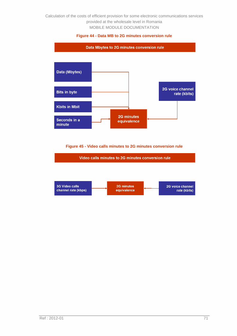
Calculation of the costs of efficient provision for some electronic communications services
provided at the wholesale level in Romania
MOBILE MODULE DOCUMENTATION
Ref : 2012-01 71
Figure 44 - Data MB to 2G minutes conversion rule
Figure 45 - Video calls minutes to 2G minutes conversion rule
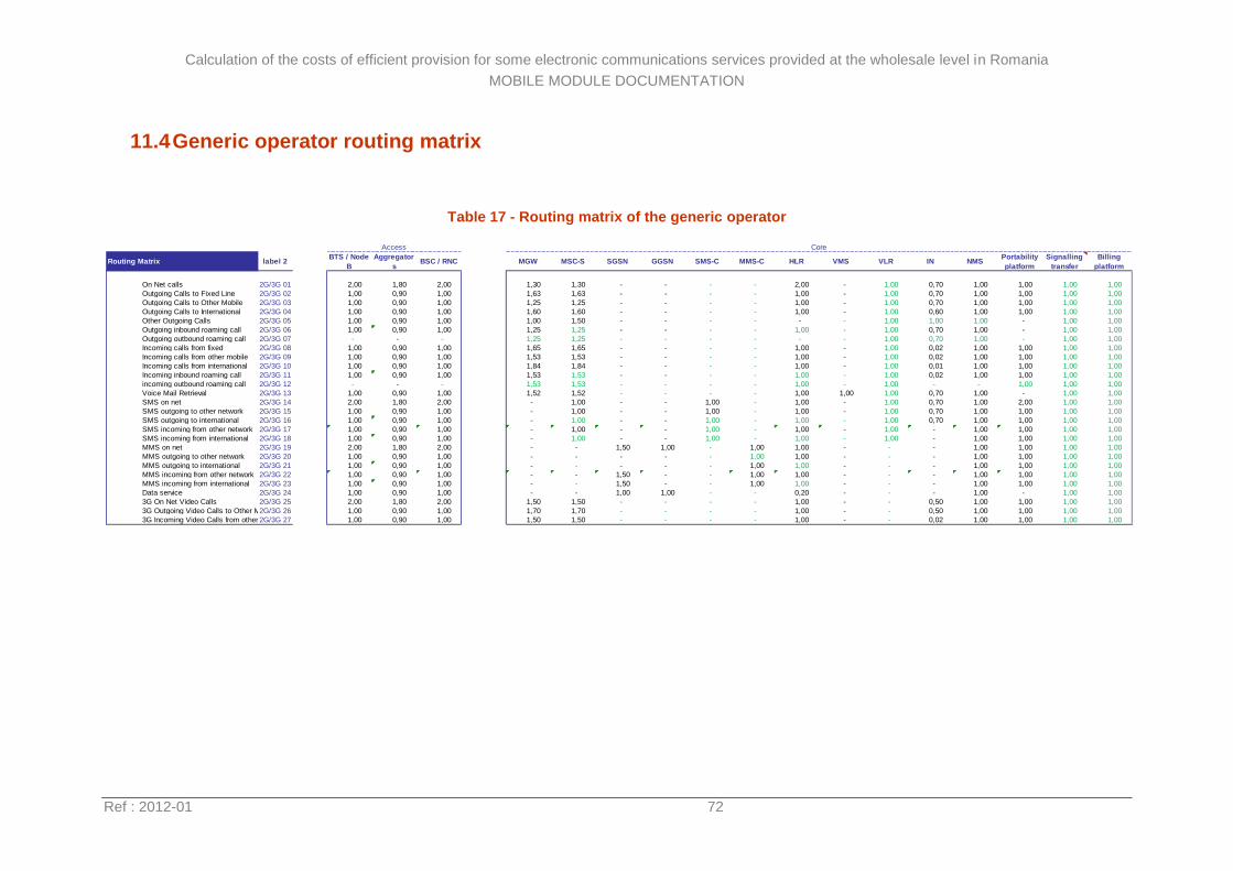
Calculation of the costs of efficient provision for some electronic communications services provided at the wholesale level in Romania
MOBILE MODULE DOCUMENTATION
Ref : 2012-01 72
11.4 Generic operator routing matrix
Table 17 - Routing matrix of the generic operator
Routing Matrix label 2BTS / Node
B
Aggregator
sBSC / RNC MGW MSC-S SGSN GGSN SMS-C MMS-C HLR VMS VLR IN NMS
Portability
platform
Signalling
transfer
Billing
platform
On Net calls 2G/3G 01 2,00 1,80 2,00 1,30 1,30 - - - - 2,00 - 1,00 0,70 1,00 1,00 1,00 1,00
Outgoing Calls to Fixed Line 2G/3G 02 1,00 0,90 1,00 1,63 1,63 - - - - 1,00 - 1,00 0,70 1,00 1,00 1,00 1,00
Outgoing Calls to Other Mobile 2G/3G 03 1,00 0,90 1,00 1,25 1,25 - - - - 1,00 - 1,00 0,70 1,00 1,00 1,00 1,00
Outgoing Calls to International 2G/3G 04 1,00 0,90 1,00 1,60 1,60 - - - - 1,00 - 1,00 0,60 1,00 1,00 1,00 1,00
Other Outgoing Calls 2G/3G 05 1,00 0,90 1,00 1,00 1,50 - - - - - - 1,00 1,00 1,00 - 1,00 1,00
Outgoing inbound roaming call 2G/3G 06 1,00 0,90 1,00 1,25 1,25 - - - - 1,00 - 1,00 0,70 1,00 - 1,00 1,00
Outgoing outbound roaming call 2G/3G 07 - - - 1,25 1,25 - - - - - - 1,00 0,70 1,00 - 1,00 1,00
Incoming calls from fixed 2G/3G 08 1,00 0,90 1,00 1,65 1,65 - - - - 1,00 - 1,00 0,02 1,00 1,00 1,00 1,00
Incoming calls from other mobile 2G/3G 09 1,00 0,90 1,00 1,53 1,53 - - - - 1,00 - 1,00 0,02 1,00 1,00 1,00 1,00
Incoming calls from international 2G/3G 10 1,00 0,90 1,00 1,84 1,84 - - - - 1,00 - 1,00 0,01 1,00 1,00 1,00 1,00
Incoming inbound roaming call 2G/3G 11 1,00 0,90 1,00 1,53 1,53 - - - - 1,00 - 1,00 0,02 1,00 1,00 1,00 1,00
incoming outbound roaming call 2G/3G 12 - - - 1,53 1,53 - - - - 1,00 - 1,00 - - 1,00 1,00 1,00
Voice Mail Retrieval 2G/3G 13 1,00 0,90 1,00 1,52 1,52 - - - - 1,00 1,00 1,00 0,70 1,00 - 1,00 1,00
SMS on net 2G/3G 14 2,00 1,80 2,00 - 1,00 - - 1,00 - 1,00 - 1,00 0,70 1,00 2,00 1,00 1,00
SMS outgoing to other network 2G/3G 15 1,00 0,90 1,00 - 1,00 - - 1,00 - 1,00 - 1,00 0,70 1,00 1,00 1,00 1,00
SMS outgoing to international 2G/3G 16 1,00 0,90 1,00 - 1,00 - - 1,00 - 1,00 - 1,00 0,70 1,00 1,00 1,00 1,00
SMS incoming from other network 2G/3G 17 1,00 0,90 1,00 - 1,00 - - 1,00 - 1,00 - 1,00 - 1,00 1,00 1,00 1,00
SMS incoming from international 2G/3G 18 1,00 0,90 1,00 - 1,00 - - 1,00 - 1,00 - 1,00 - 1,00 1,00 1,00 1,00
MMS on net 2G/3G 19 2,00 1,80 2,00 - - 1,50 1,00 - 1,00 1,00 - - - 1,00 1,00 1,00 1,00
MMS outgoing to other network 2G/3G 20 1,00 0,90 1,00 - - - - - 1,00 1,00 - - - 1,00 1,00 1,00 1,00
MMS outgoing to international 2G/3G 21 1,00 0,90 1,00 - - - - - 1,00 1,00 - - - 1,00 1,00 1,00 1,00
MMS incoming from other network 2G/3G 22 1,00 0,90 1,00 - - 1,50 - - 1,00 1,00 - - - 1,00 1,00 1,00 1,00
MMS incoming from international 2G/3G 23 1,00 0,90 1,00 - - 1,50 - - 1,00 1,00 - - - 1,00 1,00 1,00 1,00
Data service 2G/3G 24 1,00 0,90 1,00 - - 1,00 1,00 - - 0,20 - - - 1,00 - 1,00 1,00
3G On Net Video Calls 2G/3G 25 2,00 1,80 2,00 1,50 1,50 - - - - 1,00 - - 0,50 1,00 1,00 1,00 1,00
3G Outgoing Video Calls to Other Mobile2G/3G 26 1,00 0,90 1,00 1,70 1,70 - - - - 1,00 - - 0,50 1,00 1,00 1,00 1,00
3G Incoming Video Calls from other mobile2G/3G 27 1,00 0,90 1,00 1,50 1,50 - - - - 1,00 - - 0,02 1,00 1,00 1,00 1,00
Access Core
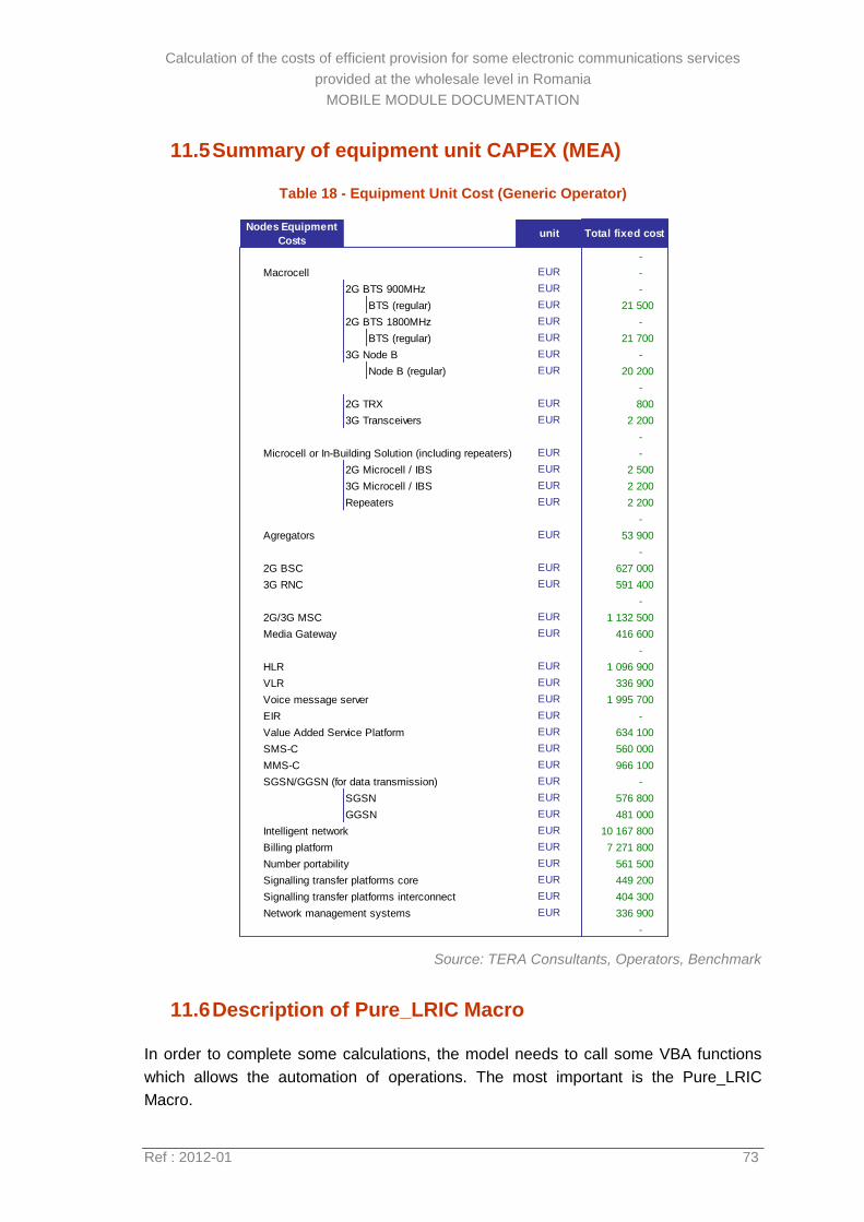
Calculation of the costs of efficient provision for some electronic communications services
provided at the wholesale level in Romania
MOBILE MODULE DOCUMENTATION
Ref : 2012-01 73
11.5 Summary of equipment unit CAPEX (MEA)
Table 18 - Equipment Unit Cost (Generic Operator)
Source: TERA Consultants, Operators, Benchmark
11.6 Description of Pure_LRIC Macro
In order to complete some calculations, the model needs to call some VBA functions
which allows the automation of operations. The most important is the Pure_LRIC
Macro.
unit Total fixed cost
-
Macrocell EUR -
2G BTS 900MHz EUR -
BTS (regular) EUR 21 500
2G BTS 1800MHz EUR -
BTS (regular) EUR 21 700
3G Node B EUR -
Node B (regular) EUR 20 200
-
2G TRX EUR 800
3G Transceivers EUR 2 200
-
Microcell or In-Building Solution (including repeaters) EUR -
2G Microcell / IBS EUR 2 500
3G Microcell / IBS EUR 2 200
Repeaters EUR 2 200
-
Agregators EUR 53 900
-
2G BSC EUR 627 000
3G RNC EUR 591 400
-
2G/3G MSC EUR 1 132 500
Media Gateway EUR 416 600
-
HLR EUR 1 096 900
VLR EUR 336 900
Voice message server EUR 1 995 700
EIR EUR -
Value Added Service Platform EUR 634 100
SMS-C EUR 560 000
MMS-C EUR 966 100
SGSN/GGSN (for data transmission) EUR -
SGSN EUR 576 800
GGSN EUR 481 000
Intelligent network EUR 10 167 800
Billing platform EUR 7 271 800
Number portability EUR 561 500
Signalling transfer platforms core EUR 449 200
Signalling transfer platforms interconnect EUR 404 300
Network management systems EUR 336 900
-
Nodes Equipment
Costs
Calculation of the costs of efficient provision for some electronic communications services
provided at the wholesale level in Romania
MOBILE MODULE DOCUMENTATION
Ref : 2012-01 74
This function calculates the pure LRIC cost of the selected services (refer to Sheet
#7.3).
The service Pure LRIC cost is the result of the division of service total cost (1st term of
the division) by the service annual traffic (2nd term of the devision).
The different steps of this function are:
Step 1: The cell ‘AG20’ of the Sheet #4.1 is set to ‘LRAIC+’ value. This means
that the model will consider all the list of services.
Step 2: The model then calculates the corresponding network cost (all services
considered).
Step 3: These network costs are then copied in values in the buffer in Sheet #6,
line 524 to 544.
Step 4: The model goes back to the cell ‘AG20’ of the Sheet #4.1, and sets it to
‘Pure LRIC inverted’. This means that the model will consider only the services
targeted by the Pure LRIC cost calculation (example: 2G terminating voice
services).
Step 5: The model then calculates the total annual commercial volume of traffic
generated by these services (2nd term of the division), in the Sheet #4.1, line
639.
Step 6: These volumes are copied in values in the Sheet #7.3, line 15.
Step 7: The model goes back to the cell ‘AG20’ of the Sheet #4.1 which is set
to ‘Pure LRIC’. This time the model will consider all the services except the
ones targeted by the Pure LRIC cost calculation.
Step 8: The model will calculate the cost of a network built in order to handle all
the services except the services targeted by the pure LRIC cost calculation.
Step 9: The model calculates the difference between the cost of a network built
to handle all the services (content of the buffer), and the cost of a network built
to handle all the services except the one targeted by the Pure LRIC cost
calculation (the last values of Sheet #6 line 499 to 519). This difference is
calculated in Sheet #6 line 550 to 570.
Step 10: This difference represents the cost of the pure LRIC increment, and is
copied in values in the Sheet #7.3, line 20 (1st term of the division).
Step 11: The model calculates the unit cost of the pure LRIC increment in
Sheet #7.3, line 25.
Step 12: the buffer in Sheet #6 line 524 to 544 is cleared.
Step 13: the model goes back to the cell ‘AG20’ of the Sheet #4.1 and set it
back to its initial value ‘LRAIC+’.