Embed Size (px)
Citation preview

2.1 Prof. Dr.-Ing. Jochen H. Schiller www.jochenschiller.de MC - 2013
Mobile Communications Chapter 2: Wireless Transmission
• Frequencies • Signals, antennas, signal propagation, MIMO • Multiplexing, Cognitive Radio • Spread spectrum, modulation • Cellular systems

2.2 Prof. Dr.-Ing. Jochen H. Schiller www.jochenschiller.de MC - 2013
Frequencies for communication • VLF = Very Low Frequency UHF = Ultra High Frequency • LF = Low Frequency SHF = Super High Frequency • MF = Medium Frequency EHF = Extra High Frequency • HF = High Frequency UV = Ultraviolet Light • VHF = Very High Frequency
• Frequency and wave length • λ = c/f • wave length λ, speed of light c ≅ 3x10⁸m/s, frequency f
1 Mm 300 Hz
10 km 30 kHz
100 m 3 MHz
1 m 300 MHz
10 mm 30 GHz
100 µm 3 THz
1 µm 300 THz
visible light VLF LF MF HF VHF UHF SHF EHF infrared UV
optical transmission coax cable twisted pair
2.3 Prof. Dr.-Ing. Jochen H. Schiller www.jochenschiller.de MC - 2013
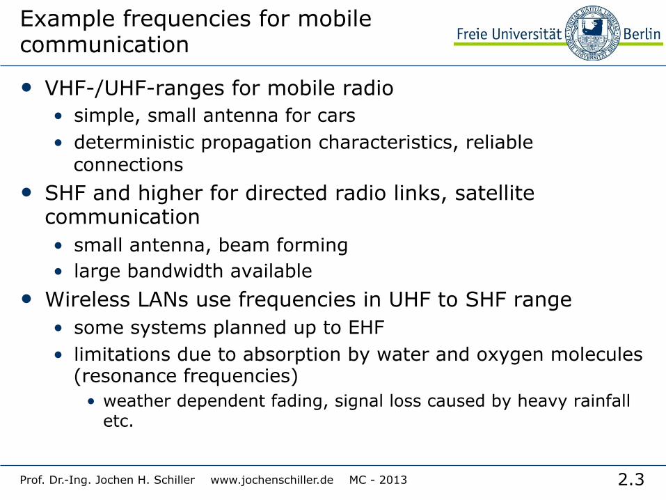
Example frequencies for mobile communication
• VHF-/UHF-ranges for mobile radio • simple, small antenna for cars • deterministic propagation characteristics, reliable
connections • SHF and higher for directed radio links, satellite
communication • small antenna, beam forming • large bandwidth available
• Wireless LANs use frequencies in UHF to SHF range • some systems planned up to EHF • limitations due to absorption by water and oxygen molecules
(resonance frequencies) • weather dependent fading, signal loss caused by heavy rainfall
etc.
2.4 Prof. Dr.-Ing. Jochen H. Schiller www.jochenschiller.de MC - 2013
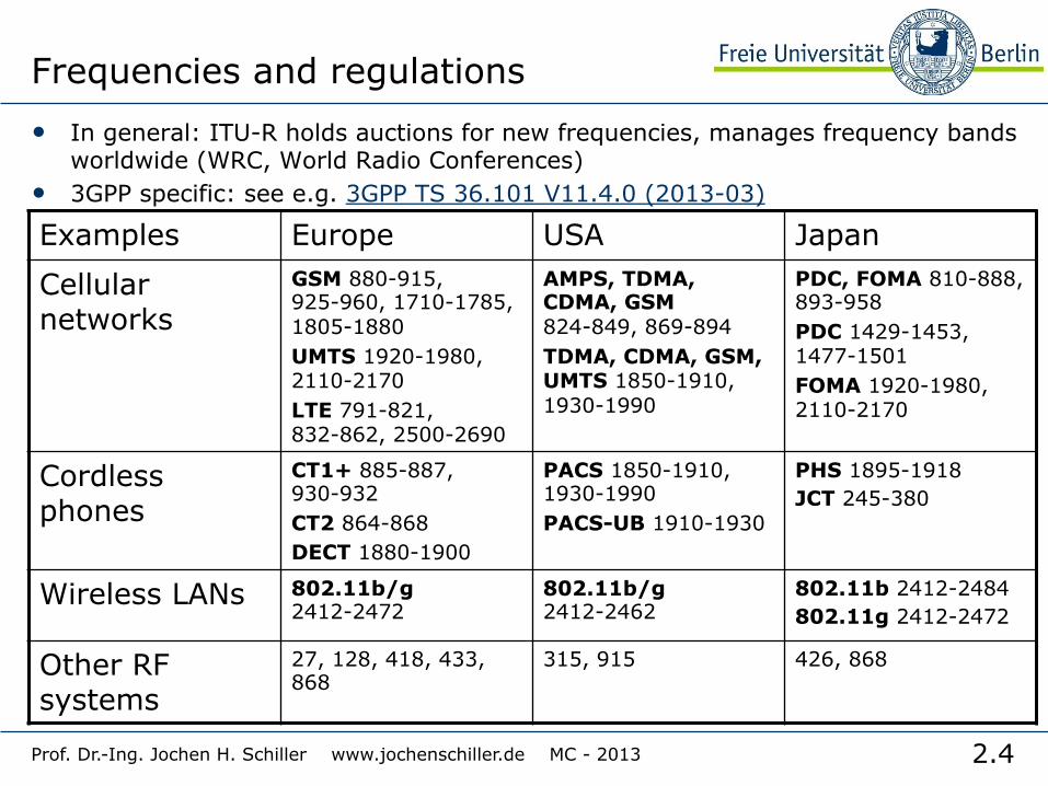
Frequencies and regulations • In general: ITU-R holds auctions for new frequencies, manages frequency bands
worldwide (WRC, World Radio Conferences) • 3GPP specific: see e.g. 3GPP TS 36.101 V11.4.0 (2013-03)
Examples Europe USA Japan
Cellular networks
GSM 880-915, 925-960, 1710-1785, 1805-1880 UMTS 1920-1980, 2110-2170 LTE 791-821, 832-862, 2500-2690
AMPS, TDMA, CDMA, GSM 824-849, 869-894 TDMA, CDMA, GSM, UMTS 1850-1910, 1930-1990
PDC, FOMA 810-888, 893-958 PDC 1429-1453, 1477-1501 FOMA 1920-1980, 2110-2170
Cordless phones
CT1+ 885-887, 930-932 CT2 864-868 DECT 1880-1900
PACS 1850-1910, 1930-1990 PACS-UB 1910-1930
PHS 1895-1918 JCT 245-380
Wireless LANs 802.11b/g 2412-2472
802.11b/g 2412-2462
802.11b 2412-2484 802.11g 2412-2472
Other RF systems
27, 128, 418, 433, 868
315, 915 426, 868

2.5 Prof. Dr.-Ing. Jochen H. Schiller www.jochenschiller.de MC - 2013
Signals I
• physical representation of data • function of time and location • signal parameters: parameters representing the value of
data • classification
• continuous time/discrete time • continuous values/discrete values • analog signal = continuous time and continuous values • digital signal = discrete time and discrete values
• signal parameters of periodic signals: period T, frequency f=1/T, amplitude A, phase shift ϕ • sine wave as special periodic signal for a carrier:
s(t) = At sin(2 π ft t + ϕt)
2.6 Prof. Dr.-Ing. Jochen H. Schiller www.jochenschiller.de MC - 2013
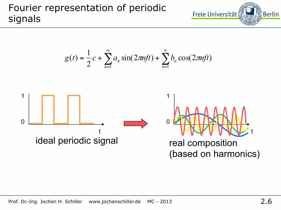
Fourier representation of periodic signals
)2cos()2sin(21)(
11
nftbnftactgn
nn
n ππ ∑∑∞
=
∞
=
++=
1
0
1
0 t t
ideal periodic signal real composition (based on harmonics)

2.7 Prof. Dr.-Ing. Jochen H. Schiller www.jochenschiller.de MC - 2013
Signals II
• Different representations of signals • amplitude (amplitude domain) • frequency spectrum (frequency domain) • phase state diagram (amplitude M and phase ϕ in polar
coordinates)
• Composed signals transferred into frequency domain using Fourier transformation
• Digital signals need • infinite frequencies for perfect transmission • modulation with a carrier frequency for transmission (analog
signal!)
f [Hz]
A [V]
ϕ
I= M cos ϕ
Q = M sin ϕ
ϕ
A [V]
t[s]

2.8 Prof. Dr.-Ing. Jochen H. Schiller www.jochenschiller.de MC - 2013
Antennas: isotropic radiator
• Radiation and reception of electromagnetic waves, coupling of wires to space for radio transmission
• Isotropic radiator: equal radiation in all directions (three dimensional) - only a theoretical reference antenna
• Real antennas always have directive effects (vertically and/or horizontally)
• Radiation pattern: measurement of radiation around an antenna
z y
x
z
y x ideal isotropic radiator

2.9 Prof. Dr.-Ing. Jochen H. Schiller www.jochenschiller.de MC - 2013
Antennas: simple dipoles
• Real antennas are not isotropic radiators but, e.g., dipoles with lengths λ/4 on car roofs or λ/2 as Hertzian dipole è shape of antenna proportional to wavelength
• Example: Radiation pattern of a simple Hertzian dipole
• Gain: maximum power in the direction of the main lobe compared to the power of an isotropic radiator (with the same average power)
side view (xy-plane)
x
y
side view (yz-plane)
z
y
top view (xz-plane)
x
z
simple dipole
λ/4 λ/2

2.10 Prof. Dr.-Ing. Jochen H. Schiller www.jochenschiller.de MC - 2013
Antennas: directed and sectorized
side view (xy-plane)
x
y
side view (yz-plane)
z
y
top view (xz-plane)
x
z
top view, 3 sector
x
z
top view, 6 sector
x
z
• Often used for microwave connections or base stations for mobile phones (e.g., radio coverage of a valley)
directed antenna
sectorized antenna

2.11 Prof. Dr.-Ing. Jochen H. Schiller www.jochenschiller.de MC - 2013
Antennas: diversity
• Grouping of 2 or more antennas • multi-element antenna arrays
• Antenna diversity • switched diversity, selection diversity
• receiver chooses antenna with largest output • diversity combining
• combine output power to produce gain • cophasing needed to avoid cancellation
+
λ/4 λ/2 λ/4
ground plane
λ/2 λ/2
+
λ/2

2.12
MIMO • Multiple-Input Multiple-Output
• Use of several antennas at receiver and transmitter • Increased data rates and transmission range without additional transmit power or
bandwidth via higher spectral efficiency, higher link robustness, reduced fading • Examples
• IEEE 802.11n, LTE, HSPA+, … • Functions
• “Beamforming”: emit the same signal from all antennas to maximize signal power at receiver antenna
• Spatial multiplexing: split high-rate signal into multiple lower rate streams and transmit over different antennas
• Diversity coding: transmit single stream over different antennas with (near) orthogonal codes
Prof. Dr.-Ing. Jochen H. Schiller www.jochenschiller.de MC - 2013
sender
receiver
t1
t2
t3
Time of flight t2=t1+d2 t3=t1+d3
1
2
3 Sending time 1: t0 2: t0-d2 3: t0-d3

2.13 Prof. Dr.-Ing. Jochen H. Schiller www.jochenschiller.de MC - 2013
Signal propagation ranges
• Transmission range • communication possible • low error rate
• Detection range • detection of the signal
possible • no communication
possible • Interference range
• signal may not be detected
• signal adds to the background noise
• Warning: figure misleading – bizarre shaped, time-varying ranges in reality!
distance
sender
transmission
detection
interference

2.14 Prof. Dr.-Ing. Jochen H. Schiller www.jochenschiller.de MC - 2013
Signal propagation
• Propagation in free space always like light (straight line) • Receiving power proportional to 1/d² in vacuum – much more in
real environments, e.g., d3.5…d4 (d = distance between sender and receiver)
• Receiving power additionally influenced by • fading (frequency dependent) • shadowing • reflection at large obstacles • refraction depending on the density of a medium • scattering at small obstacles • diffraction at edges
reflection scattering diffraction shadowing refraction

2.15 Prof. Dr.-Ing. Jochen H. Schiller www.jochenschiller.de MC - 2013
Real world examples
www.ihe.kit.edu/index.php

2.16 Prof. Dr.-Ing. Jochen H. Schiller www.jochenschiller.de MC - 2013
Multipath propagation
• Signal can take many different paths between sender and receiver due to reflection, scattering, diffraction
• Time dispersion: signal is dispersed over time • interference with “neighbor” symbols, Inter Symbol
Interference (ISI) • The signal reaches a receiver directly and phase shifted
• distorted signal depending on the phases of the different parts
signal at sender signal at receiver
LOS pulses multipath pulses
LOS (line-of-sight)
2.17 Prof. Dr.-Ing. Jochen H. Schiller www.jochenschiller.de MC - 2013
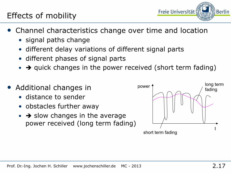
Effects of mobility
• Channel characteristics change over time and location • signal paths change • different delay variations of different signal parts • different phases of signal parts • è quick changes in the power received (short term fading)
• Additional changes in • distance to sender • obstacles further away • è slow changes in the average
power received (long term fading) short term fading
long term fading
t
power

2.18 Prof. Dr.-Ing. Jochen H. Schiller www.jochenschiller.de MC - 2013
• Multiplexing in 4 dimensions • space (si) • time (t) • frequency (f) • code (c)
• Goal: multiple use of a shared medium
• Important: guard spaces needed!
s2
s3
s1
Multiplexing
f
t
c
k2 k3 k4 k5 k6 k1
f
t
c
f
t
c
channels ki

2.19 Prof. Dr.-Ing. Jochen H. Schiller www.jochenschiller.de MC - 2013
Frequency multiplex
• Separation of the whole spectrum into smaller frequency bands
• A channel gets a certain band of the spectrum for the whole time
• Advantages • no dynamic coordination
necessary • works also for analog signals
• Disadvantages • waste of bandwidth
if the traffic is distributed unevenly
• inflexible
k2 k3 k4 k5 k6 k1
f
t
c

2.20 Prof. Dr.-Ing. Jochen H. Schiller www.jochenschiller.de MC - 2013
f
t
c
k2 k3 k4 k5 k6 k1
Time multiplex
• A channel gets the whole spectrum for a certain amount of time
• Advantages • only one carrier in the
medium at any time • throughput high even
for many users
• Disadvantages • precise
synchronization necessary

2.21 Prof. Dr.-Ing. Jochen H. Schiller www.jochenschiller.de MC - 2013
f
Time and frequency multiplex
• Combination of both methods • A channel gets a certain frequency band for a certain
amount of time • Example: GSM
• Advantages • better protection against
tapping • protection against frequency
selective interference • but: precise coordination
required
t
c
k2 k3 k4 k5 k6 k1

2.22
Cognitive Radio
• Typically in the form of a spectrum sensing CR • Detect unused spectrum and share with others avoiding interference • Choose automatically best available spectrum (intelligent form of time/
frequency/space multiplexing) • Distinguish
• Primary Users (PU): users assigned to a specific spectrum by e.g. regulation • Secondary Users (SU): users with a CR to use unused spectrum
• Examples • Reuse of (regionally) unused analog TV spectrum (aka white space) • Temporary reuse of unused spectrum e.g. of pagers, amateur radio etc.
Prof. Dr.-Ing. Jochen H. Schiller www.jochenschiller.de MC - 2013
space mux frequency/time mux
PU PU
PU PU SU
SU
SU
SU
f
t
PU
PU
PU PU PU PU
PU SU
SU SU
SU SU SU

2.23 Prof. Dr.-Ing. Jochen H. Schiller www.jochenschiller.de MC - 2013
Code multiplex
• Each channel has a unique code
• All channels use the same spectrum at the same time
• Advantages • bandwidth efficient • no coordination and synchronization
necessary • good protection against interference
and tapping • Disadvantages
• varying user data rates • more complex signal regeneration
• Implemented using spread spectrum technology
k2 k3 k4 k5 k6 k1
f
t
c

2.24 Prof. Dr.-Ing. Jochen H. Schiller www.jochenschiller.de MC - 2013
Modulation
• Digital modulation • digital data is translated into an analog signal (baseband) • ASK, FSK, PSK - main focus in this chapter • differences in spectral efficiency, power efficiency, robustness
• Analog modulation • shifts center frequency of baseband signal up to the radio carrier
• Motivation • smaller antennas (e.g., λ/4) • Frequency Division Multiplexing • medium characteristics
• Basic schemes • Amplitude Modulation (AM) • Frequency Modulation (FM) • Phase Modulation (PM)

2.25 Prof. Dr.-Ing. Jochen H. Schiller www.jochenschiller.de MC - 2013
Modulation and demodulation
synchronization decision
digital data analog
demodulation
radio carrier
analog baseband signal
101101001 radio receiver
digital modulation
digital data analog
modulation
radio carrier
analog baseband signal
101101001 radio transmitter

2.26 Prof. Dr.-Ing. Jochen H. Schiller www.jochenschiller.de MC - 2013
Digital modulation
• Modulation of digital signals known as Shift Keying • Amplitude Shift Keying (ASK):
• very simple • low bandwidth requirements • very susceptible to interference
• Frequency Shift Keying (FSK):
• needs larger bandwidth
• Phase Shift Keying (PSK): • more complex • robust against interference
1 0 1
t
1 0 1
t
1 0 1
t

2.27 Prof. Dr.-Ing. Jochen H. Schiller www.jochenschiller.de MC - 2013
Advanced Frequency Shift Keying
• bandwidth needed for FSK depends on the distance between the carrier frequencies
• special pre-computation avoids sudden phase shifts è MSK (Minimum Shift Keying) • bit separated into even and odd bits, the duration of each bit
is doubled • depending on the bit values (even, odd) the higher or lower
frequency, original or inverted is chosen • the frequency of one carrier is twice the frequency of the
other • Equivalent to offset QPSK
• even higher bandwidth efficiency using a Gaussian low-pass filter è GMSK (Gaussian MSK), used in GSM

2.28 Prof. Dr.-Ing. Jochen H. Schiller www.jochenschiller.de MC - 2013
Example of MSK
data
even bits
odd bits
1 1 1 1 0 0 0
t
low frequency
high frequency
MSK signal
bit
even 0 1 0 1
odd 0 0 1 1
signal h n n h value - - + +
h: high frequency n: low frequency +: original signal -: inverted signal
No phase shifts!

2.29 Prof. Dr.-Ing. Jochen H. Schiller www.jochenschiller.de MC - 2013
Advanced Phase Shift Keying • BPSK (Binary Phase Shift
Keying): • bit value 0: sine wave • bit value 1: inverted sine wave • very simple PSK • low spectral efficiency • robust, used e.g. in satellite
systems • QPSK (Quadrature Phase Shift
Keying): • 2 bits coded as one symbol • symbol determines shift of sine
wave • needs less bandwidth compared
to BPSK • more complex
• Often also transmission of relative, not absolute phase shift: DQPSK - Differential QPSK (IS-136, PHS) 11 10 00 01
Q
I 0 1
Q
I
11
01
10
00
A
t

2.30 Prof. Dr.-Ing. Jochen H. Schiller www.jochenschiller.de MC - 2013
Quadrature Amplitude Modulation
• Quadrature Amplitude Modulation (QAM) • combines amplitude and phase modulation • it is possible to code n bits using one symbol • 2n discrete levels, n=2 identical to QPSK
• Bit error rate increases with n, but less errors compared to comparable PSK schemes • Example: 16-QAM (4 bits = 1 symbol) • Symbols 0011 and 0001 have
the same phase φ, but different amplitude a. 0000 and 1000 have different phase, but same amplitude.
0000
0001
0011
1000
Q
I
0010
φ
a

2.31 Prof. Dr.-Ing. Jochen H. Schiller www.jochenschiller.de MC - 2013
Hierarchical Modulation
• DVB-T modulates two separate data streams onto a single DVB-T stream
• High Priority (HP) embedded within a Low Priority (LP) stream
• Multi carrier system, about 2000 or 8000 carriers • QPSK, 16 QAM, 64QAM • Example: 64QAM
• good reception: resolve the entire 64QAM constellation
• poor reception, mobile reception: resolve only QPSK portion
• 6 bit per QAM symbol, 2 most significant determine QPSK
• HP service coded in QPSK (2 bit), LP uses remaining 4 bit
Q
I
00
10
000010 010101

2.32 Prof. Dr.-Ing. Jochen H. Schiller www.jochenschiller.de MC - 2013
Spread spectrum technology
• Problem of radio transmission: frequency dependent fading can wipe out narrow band signals for duration of the interference
• Solution: spread the narrow band signal into a broad band signal using a special code • protection against narrow band interference
• Side effects: • coexistence of several signals without dynamic coordination • tap-proof
• Alternatives: Direct Sequence, Frequency Hopping
detection at receiver
interference spread signal
signal
spread interference
f f
power power

2.33 Prof. Dr.-Ing. Jochen H. Schiller www.jochenschiller.de MC - 2013
Effects of spreading and interference
dP/df
f i)
dP/df
f ii)
sender
dP/df
f iii)
dP/df
f iv)
receiver f
v)
user signal broadband interference narrowband interference
dP/df

2.34 Prof. Dr.-Ing. Jochen H. Schiller www.jochenschiller.de MC - 2013
Spreading and frequency selective fading
frequency
channel quality
1 2 3
4
5 6
narrow band signal
guard space
2 2
2 2
2
frequency
channel quality
1
spread spectrum
narrowband channels
spread spectrum channels

2.35 Prof. Dr.-Ing. Jochen H. Schiller www.jochenschiller.de MC - 2013
DSSS (Direct Sequence Spread Spectrum) I
• XOR of the signal with pseudo-random number (chipping sequence) • many chips per bit (e.g., 128) result in higher bandwidth of
the signal • Advantages
• reduces frequency selective fading
• in cellular networks • base stations can use the
same frequency range • several base stations can
detect and recover the signal • soft handover
• Disadvantages • precise power control necessary
user data
chipping sequence
resulting signal
0 1
0 1 1 0 1 0 1 0 1 0 0 1 1 1
XOR
0 1 1 0 0 1 0 1 1 0 1 0 0 1
=
tb
tc
tb: bit period tc: chip period

2.36 Prof. Dr.-Ing. Jochen H. Schiller www.jochenschiller.de MC - 2013
DSSS (Direct Sequence Spread Spectrum) II
X user data
chipping sequence
modulator
radio carrier
spread spectrum signal
transmit signal
transmitter
demodulator
received signal
radio carrier
X
chipping sequence
lowpass filtered signal
receiver
integrator
products
decision data
sampled sums
correlator
2.37 Prof. Dr.-Ing. Jochen H. Schiller www.jochenschiller.de MC - 2013
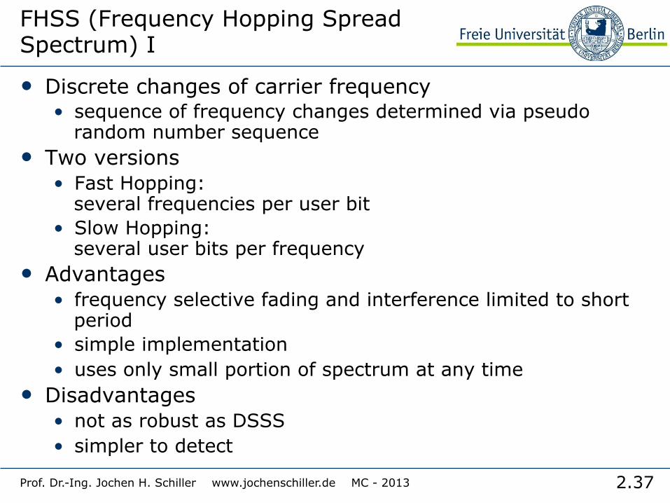
FHSS (Frequency Hopping Spread Spectrum) I
• Discrete changes of carrier frequency • sequence of frequency changes determined via pseudo
random number sequence • Two versions
• Fast Hopping: several frequencies per user bit
• Slow Hopping: several user bits per frequency
• Advantages • frequency selective fading and interference limited to short
period • simple implementation • uses only small portion of spectrum at any time
• Disadvantages • not as robust as DSSS • simpler to detect
2.38 Prof. Dr.-Ing. Jochen H. Schiller www.jochenschiller.de MC - 2013
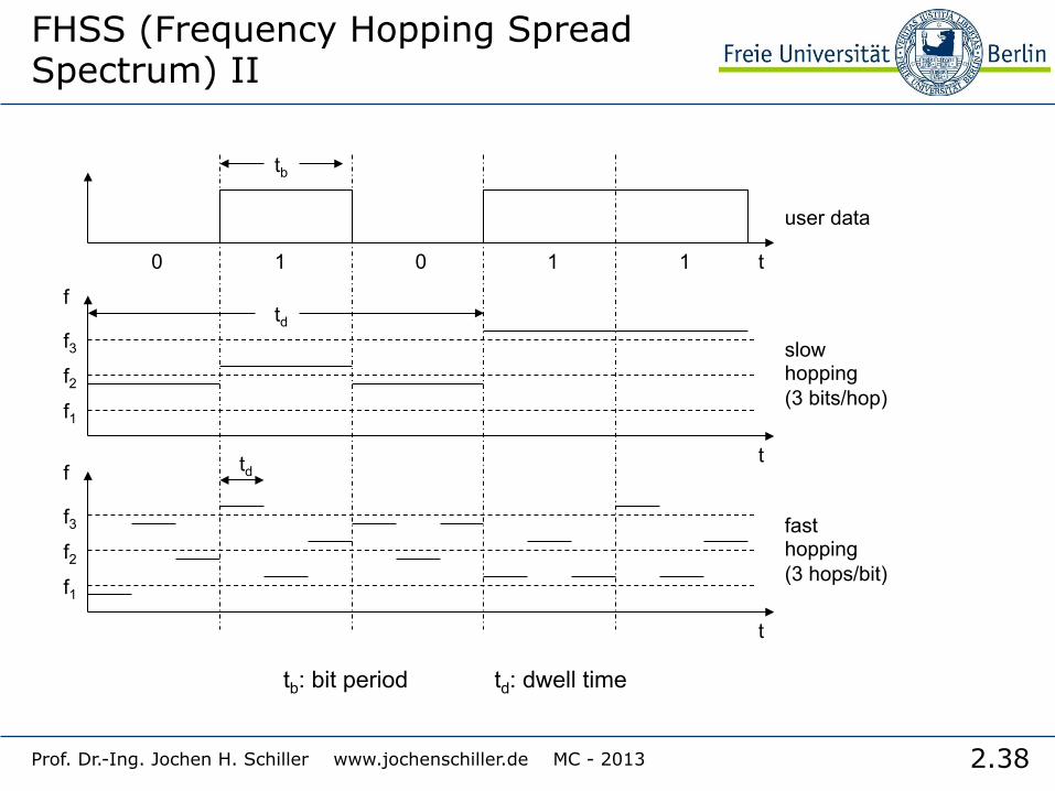
FHSS (Frequency Hopping Spread Spectrum) II
user data
slow hopping (3 bits/hop)
fast hopping (3 hops/bit)
0 1
tb
0 1 1 t
f
f1
f2
f3
t
td
f
f1
f2
f3
t
td
tb: bit period td: dwell time

2.39 Prof. Dr.-Ing. Jochen H. Schiller www.jochenschiller.de MC - 2013
FHSS (Frequency Hopping Spread Spectrum) III
modulator user data
hopping sequence
modulator
narrowband signal spread
transmit signal
transmitter
received signal
receiver
demodulator data
frequency synthesizer
hopping sequence
demodulator
frequency synthesizer
narrowband signal

2.40
Software Defined Radio
• Basic idea (ideal world) • Full flexibility wrt modulation, carrier frequency, coding… • Simply download a new radio! • Transmitter: digital signal processor plus very fast D/A-converter • Receiver: very fast A/D-converter plus digital signal processor
• Real world • Problems due to interference, high accuracy/high data rate, low-noise
amplifiers needed, filters etc. • Examples
• Joint Tactical Radio System • GNU Radio, Universal Software Radio Peripheral, …
Prof. Dr.-Ing. Jochen H. Schiller www.jochenschiller.de MC - 2013
Application Signal Processor D/A Converter
Application Signal Processor A/D Converter
2.41 Prof. Dr.-Ing. Jochen H. Schiller www.jochenschiller.de MC - 2013
Cell structure
• Implements space division multiplex • base station covers a certain transmission area (cell)
• Mobile stations communicate only via the base station
• Advantages of cell structures • higher capacity, higher number of users • less transmission power needed • more robust, decentralized • base station deals with interference, transmission area etc. locally
• Problems • fixed network needed for the base stations • handover (changing from one cell to another) necessary • interference with other cells
• Cell sizes from some 100 m in cities to, e.g., 35 km on the country side (GSM) - even less for higher frequencies

2.42 Prof. Dr.-Ing. Jochen H. Schiller www.jochenschiller.de MC - 2013
Frequency planning I
• Frequency reuse only with a certain distance between the base stations
• Standard model using 7 frequencies:
• Fixed frequency assignment: • certain frequencies are assigned to a certain cell • problem: different traffic load in different cells
• Dynamic frequency assignment: • base station chooses frequencies depending on the
frequencies already used in neighbor cells • more capacity in cells with more traffic • assignment can also be based on interference measurements
f4 f5
f1 f3
f2
f6
f7
f3 f2
f4 f5
f1

2.43 Prof. Dr.-Ing. Jochen H. Schiller www.jochenschiller.de MC - 2013
Frequency planning II
f1 f2
f3 f2
f1
f1
f2
f3 f2
f3 f1
f2 f1
f3 f3
f3 f3
f3
f4 f5
f1 f3
f2
f6
f7
f3 f2
f4 f5
f1 f3
f5 f6
f7 f2
f2
f1 f1 f1 f2 f3
f2 f3
f2 f3 h1
h2 h3 g1
g2 g3
h1 h2 h3 g1
g2 g3
g1 g2 g3
3 cell cluster
7 cell cluster
3 cell cluster with 3 sector antennas

2.44 Prof. Dr.-Ing. Jochen H. Schiller www.jochenschiller.de MC - 2013
Cell breathing
• CDM systems: cell size depends on current load • Additional traffic appears as noise to other users • If the noise level is too high users drop out of cells