MM5 Optimization Experiences and

Numerical Sensitivities Found in Convective/Non-Convective

Cloud Interactions

• Carlie J. Coats, Jr., MCNC (coats@ncsc.org)

• John N. McHenry, MCNC (mchenry@ncsc.org)• Elizabeth Hayes, SGI (eah@sgi.com)

Introduction

• MM5 Optimization for Microprocessor/Parallel Systems

• Started from MM5V2.[7,12]-GSPBL

• Speedups so far: 1.4 on SGI, 1.9 on Linux/X86, 2.36 on IBM SP

• Tiny numerical changes cause gross changes in the output

– (but these seem to be unbiased)

• Causative mechanisms include convective triggering

– inherent problem; this is ill-conditioned in nature

• Need to be careful with algorithmic formulations and optimizations

– will not be fixed simply by improved compiler technology

Optimization For Microprocessor/Parallel

• Processor characteristics:

– Pipelining and Superscalarity—need lots of independent work

– Hierarchical memory organization with registers and caches

• Solutions:

– Data structure transformations

– Logic and loop re-factoring

– Expensive-operation avoidance

– Minimize and optimize memory traffic

Pipelining and Superscalarity

• Modern microprocessors try to have multiple instructions in different stages of execution on each FPU or ALU at the same time.

• Dependencies between instructions (where one needs to complete before another can start) stall the system.

• Current technology: 20-30 instructions "in flight" at one time; even more (50+?) instructions in the future.

• Standard solutions: need lots of “independent work” to fill pipelines

– Loop unrolling for vectorizable loops (some compilers can do this)

– Loop jamming, so that there are long loop bodies with lots of independent work (some compilers can do some of this)

– Logic refactoring, so that IFs are outside the loops, not inside (compilers can NOT do this)

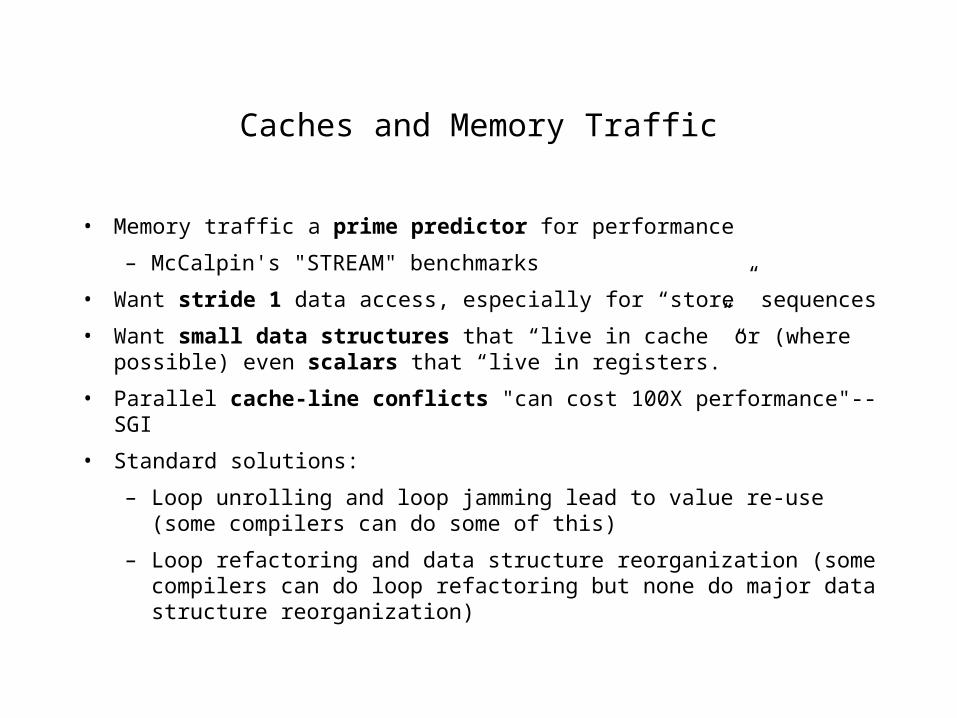
Caches and Memory Traffic

• Memory traffic a prime predictor for performance

– McCalpin's "STREAM" benchmarks

• Want stride 1 data access, especially for “store” sequences

• Want small data structures that “live in cache” or (where possible) even scalars that “live in registers.”

• Parallel cache-line conflicts "can cost 100X performance"--SGI

• Standard solutions:

– Loop unrolling and loop jamming lead to value re-use (some compilers can do some of this)

– Loop refactoring and data structure reorganization (some compilers can do loop refactoring but none do major data structure reorganization)

Expensive Operations

• Use of X**0.5 instead of SQRT(X) (this is also less accurate)

• use of divides and reciprocals

– we can see even examples of X=A/B/C/D in the code, instead of X=A/(B*C*D)

– use RPS* variables

– rationalize fractions

• EXP(A)*EXP(B) vs. EXP(A+B) (happens in LWRAD)

• repeated calculations of the same trig or log functions (happens in SOUND)

Logic Re-Factoring

•Simplified example adapted from MRFPBL:DO K=1,KLDO I=1,ILX QX(I,K) =QVB(I,J,K)*RPSB(I,J) QCX(I,K)=0. QIX(I,K)=0.END DOEND DOIF ( IMOIST(IN).NE.1)THEN DO K=1,KL DO I=1,ILX QCX(I,K)=QCB(I,J,K)*RPSB(I,J) IF(IICE.EQ.1)QIX(I,K)=QIB(I,J,K)*RPSB(I,J) END DO END DOEND IF

• IF ( IMOIST(IN).EQ.1)THEN• DO K=1,KL• DO I=1,ILX• QX(I,K) =QVB(I,J,K)*RPSB(I,J)• QCX(I,K)=0.• QIX(I,K)=0.• END DO• END DO• ELSE IF ( IICE.NE.1)THEN ! where imoist.ne.1:• DO K=1,KL• DO I=1,ILX• QX(I,K) =QVB(I,J,K)*RPSB(I,J)• QCX(I,K)=QCB(I,J,K)*RPSB(I,J)• QIX(I,K)=0.• END DO• END DO• ELSE ! imoist.ne.1 and iice.eq.1• DO K=1,KL• DO I=1,ILX• QX(I,K) =QVB(I,J,K)*RPSB(I,J)• QCX(I,K)=QCB(I,J,K)*RPSB(I,J)• QIX(I,K)=QIB(I,J,K)*RPSB(I,J)• END DO• END DO• END IF

EXMOISS Optimizations

• Inside the (innermost) miter loop:RGV(K) =AMAX1( RGV(K)/DSIGMA(K), RGV(K-1)/DSIGMA(K-1) )*DSIGMA(K)RGVC(K)=AMAX1(RGVC(K)/DSIGMA(K),RGVC(K-1)/DSIGMA(K-1) )*DSIGMA(K)

• Equivalent toDSRAT(K)=DSIGMA(K)/DSIGMA(K-1)) !! K-only pre-calculation…..RGV(K) =AMAX1( RGV(K), RGV(K-1)*DSRAT(K) )RGVC(K)=AMAX1(RGVC(K), RGVC(K-1)*DSRAT(K) )

• Rewrite loop structure and arrays as follows:

– outermost I-loop, enclosing– sequence of K-loops, then– miter loop, enclosing internal K-loop– working arrays subscripted by K only (or are scalars, when possible)

EXMOISS Optimizations, cont’d

• Rain-accumulation numerics:

– original adds one miter-step of one layer of rain to 2-D array of cumulative rain totals; serious truncation error for long runs.

– Optimized version adds up vertical-column advection-step total in a scalar; then adds that scalar to the cumulative total—better round-off, less memory traffic.

• New version is twice as fast, greatly reduced round-off errors

• Generates noticeably different MM5 model results

– no evident bias in the changed results

– caused/amplified by interaction with convective cloud parameterizations?

– See plots to come

24 Hour Forecast Grid RMS RN

0.00E+00

2.00E-01

4.00E-01

6.00E-01

8.00E-01

1.00E+00

1.20E+00

1.40E+00

1.60E+00

1 3 5 7 9

11

13

15

17

19

21

23

25

27

29

31

33

35

37

39

41

43

45

47

49

Half-Hour Time Steps

ce

nti

me

ters

Day 89 Day 90 Day 91 Day 92 Day 94 Day 95 Day 96 Day 97

24-Hour Forecasts -- Grid RMS difference: KFTOP Base - Optimized

0.00E+00

2.00E+02

4.00E+02

6.00E+02

8.00E+02

1.00E+03

1.20E+03

1.40E+03

1.60E+03

1.80E+031 3 5 7 9

11

13

15

17

19

21

23

25

27

29

31

33

35

37

39

41

43

45

47

49

Half-Hour Time Steps

Me

ters

Day 89 Day 90 Day 91 Day 92 Day 94 Day 95 Day 96 Day 97

24-Hour Forecasts -- Grid AVERAGE difference: KFTOPBase - Optimized

-3.00E+01

-2.00E+01

-1.00E+01

0.00E+00

1.00E+01

2.00E+01

3.00E+01

4.00E+01

5.00E+011 3 5 7 9 11 13 15 17 19 21 23 25 27 29 31 33 35 37 39 41 43 45 47 49

Half-Hour Time Steps

Me

ters

Day 89 Day 90 Day 91 Day 92 Day 94 Day 95 Day 96 Day 97

24-Hour Forecasts -- Grid MAX Difference RN: Base - Optimized

0.00E+00

5.00E-01

1.00E+00

1.50E+00

2.00E+00

2.50E+00

1 3 5 7 9 11 13 15 17 19 21 23 25 27 29 31 33 35 37 39 41 43 45 47 49

Half-Hour Time Steps

cen

tim

eter

s

Day 89 Day 90 Day 91 Day 92 Day 94 Day 95 Day 96 Day 97

24-Hour Forecast -- Grid MIN Difference RN: Base - Optimized

-2.50E+00

-2.00E+00

-1.50E+00

-1.00E+00

-5.00E-01

0.00E+00

1 3 5 7 9

11

13

15

17

19

21

23

25

27

29

31

33

35

37

39

41

43

45

47

49

Half-Hour Time Steps

cen

tim

eter

s

Day 89 Day 90 Day 91 Day 92 Day 94 Day 95 Day 96 Day 97

24 Hour Forecast Grid RMS Difference RN: Base - Optimized

0.00E+00

1.00E-02

2.00E-02

3.00E-02

4.00E-02

5.00E-02

6.00E-02

7.00E-02

8.00E-02

9.00E-02

1.00E-01

1 3 5 7 9

11

13

15

17

19

21

23

25

27

29

31

33

35

37

39

41

43

45

47

49

Half-Hour Time Steps

cen

tim

eter

s

Day 89 Day 90 Day 91 Day 92 Day 94 Day 95 Day 96 Day 97

24-Hour Forecast Grid MEAN Difference RN: Base - Optimized

-1.50E-03

-1.00E-03

-5.00E-04

0.00E+00

5.00E-04

1.00E-03

1.50E-03

1 3 5 7 9

11

13

15

17

19

21

23

25

27

29

31

33

35

37

39

41

43

45

47

49

Half-Hour Time Steps

cen

tim

eter

s

Day 89 Day 90 Day 91 Day 92 Day 94 Day 95 Day 96 Day 97

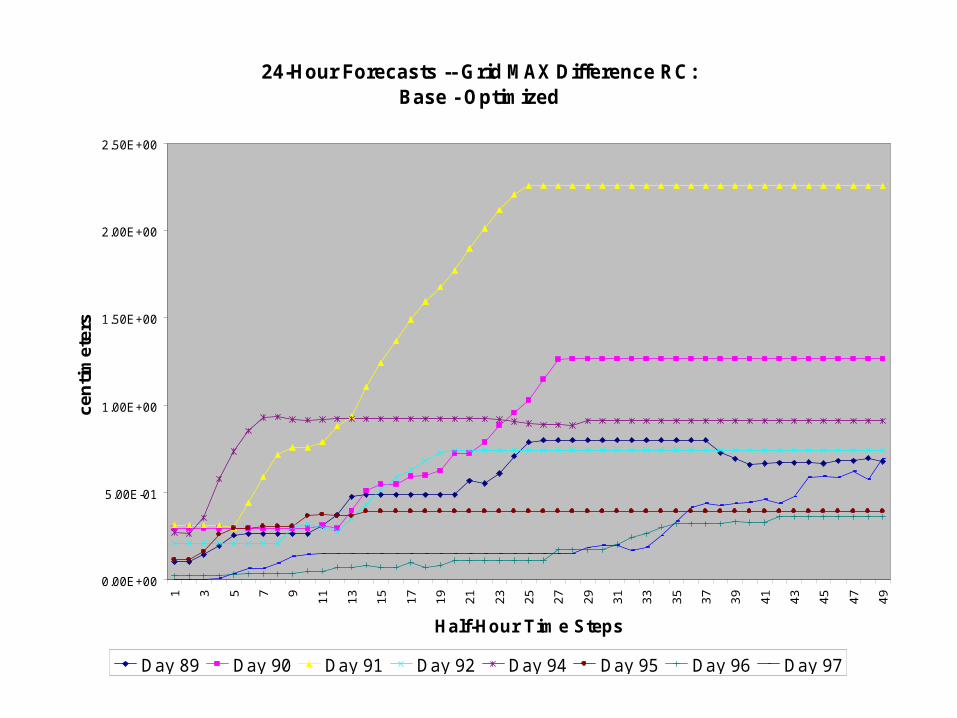
24-Hour Forecasts -- Grid MAX Difference RC: Base - Optimized

0.00E+00

5.00E-01

1.00E+00

1.50E+00

2.00E+00

2.50E+00

1 3 5 7 9

11

13

15

17

19

21

23

25

27

29

31

33

35

37

39

41

43

45

47

49

Half-Hour Time Steps

cen

tim

eter

s

Day 89 Day 90 Day 91 Day 92 Day 94 Day 95 Day 96 Day 97

24 Hour Forecast Grid RMS Difference RC Base - Optimized

0.00E+00

1.00E-02

2.00E-02

3.00E-02

4.00E-02

5.00E-02

6.00E-02

7.00E-02

8.00E-02

9.00E-02

1 3 5 7 9

11

13

15

17

19

21

23

25

27

29

31

33

35

37

39

41

43

45

47

49

Half-Hour Time Steps

cen

tim

eter

s

Day 89 Day 90 Day 91 Day 92 Day 94 Day 95 Day 96 Day 97

24-Hour Forecast Grid MEAN Difference RC: Base - Optimized

-1.00E-03

-8.00E-04

-6.00E-04

-4.00E-04

-2.00E-04

0.00E+00

2.00E-04

4.00E-04

6.00E-04

8.00E-04

1 3 5 7 9

11

13

15

17

19

21

23

25

27

29

31

33

35

37

39

41

43

45

47

49

Half-Hour Time Steps

cen

tim

eter

s

Day 89 Day 90 Day 91 Day 92 Day 94 Day 95 Day 96 Day 97

Other Routines

• Routines:

SOUND, SOLVE3, EXMOISS, GSPBL, LWRAD, MRFPBL, HADV, VADV

• Typical speedup factors for these routines

– 1.1-1.6 on SGI,

– 1.5-2.1 (but 2.54 for GSPBL) on IBM SP

• Frequently, optimized versions have reduced round-off

• Some optimizations will improve both vector a microprocessor performance

• Side effects: reduced cache footprint in EXMOISS, MRFPBL caused 5-8% speedup in SOUND, SOLVE3 on SGI Octane! (less effect on O-2000)

Food for Thought

• What does all this—especially the numerical sensitivities—say for future model formulations such as WRF?

– Double-precision-only model? (and best-available values for physics constants!)

– Ensemble forecasts? (These are very easy to achieve with the current MM5—just multiply some state variable by PSA, then by RPSA! )

– (Most radically) stochastic models that predict cell means and variances instead of deterministic point-values? (Due to theorems in integral operator theory, these have better stability and continuity properties than today’s deterministic models but sub-gridscale processes will be a challenge to formulate!)