Mixtures of Rasch Models with R Packagepsychomix

Hannah Frick, Carolin Strobl, Friedrich Leisch, Achim Zeileis

http://eeecon.uibk.ac.at/~frick/

Outline

Rasch model

Mixture models

Rasch mixture models

Illustration: Simulated data

Application: Verbal aggression

Introduction

Latent traits measured through probabilistic models for itemresponse data.

Here, Rasch model for binary items.

Crucial assumption of measurement invariance: All items measurethe latent trait in the same way for all subjects.

Check for heterogeneity in (groups of) subjects, either based onobserved covariates or unobserved latent classes.

Mixtures of Rasch models to address heterogeneity in latentclasses.

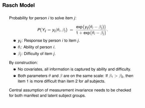
Rasch Model

Probability for person i to solve item j :

P(Yij = yij |θi , βj) =exp{yij(θi − βj)}1 + exp{θi − βj}

.

yij : Response by person i to item j .

θi : Ability of person i .

βj : Difficulty of item j .

By construction:

No covariates, all information is captured by ability and difficulty.

Both parameters θ and β are on the same scale: If β1 > β2, thenitem 1 is more difficult than item 2 for all subjects.

Central assumption of measurement invariance needs to be checkedfor both manifest and latent subject groups.

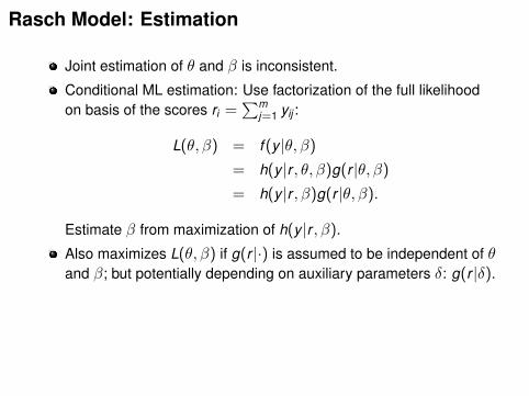
Rasch Model: Estimation

Joint estimation of θ and β is inconsistent.

Conditional ML estimation: Use factorization of the full likelihoodon basis of the scores ri =

∑mj=1 yij :

L(θ, β) = f (y |θ, β)

= h(y |r , θ, β)g(r |θ, β)

= h(y |r , β)g(r |θ, β).

Estimate β from maximization of h(y |r , β).

Also maximizes L(θ, β) if g(r |·) is assumed to be independent of θand β; but potentially depending on auxiliary parameters δ: g(r |δ).

Mixture Models

Assumption: Data stems from different classes but classmembership is unknown.

Modeling tool: Mixture models.

Mixture model =∑

weight × component.

Components represent the latent classes. They are densities or(regression) models.

Weights are a priori probabilities for the components/classes,treated either as parameters or modeled through concomitantvariables.

Rasch Mixture Models: Framework

Full mixture:

Weights: Either (non-parametric) prior probabilities πk orweights π(k |x , α) based on concomitant variables x , e.g., amultinomial logit model.

Components: Conditional likelihood for item parameters andspecification of score probabilities

f (y |π, α, β, δ) =n∏

i=1

K∑k=1

π(k |xi , α) h(yi |ri , βk ) g(ri |δk ).

Estimation of all parameters via ML through the EM algorithm.

Rasch Mixture Models: Score Probabilities

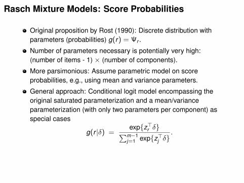
Original proposition by Rost (1990): Discrete distribution withparameters (probabilities) g(r) = Ψr .

Number of parameters necessary is potentially very high:(number of items - 1) × (number of components).

More parsimonious: Assume parametric model on scoreprobabilities, e.g., using mean and variance parameters.

General approach: Conditional logit model encompassing theoriginal saturated parameterization and a mean/varianceparameterization (with only two parameters per component) asspecial cases

g(r |δ) =exp{z>r δ}∑m−1

j=1 exp{z>j δ}.

Rasch Mixture Models: Score Probabilities

Saturated score model:

Pro: Can capture all score distributions, i.e., never misspecified.

Con: Needs many (nuisance) parameters, i.e., challenging inmodel estimation/selection.

Mean-variance score model:

Pro: Parsimonious, i.e., convenient for model estimation/selection.

Con: Potentially misspecified, e.g., for multi-modal distributions.

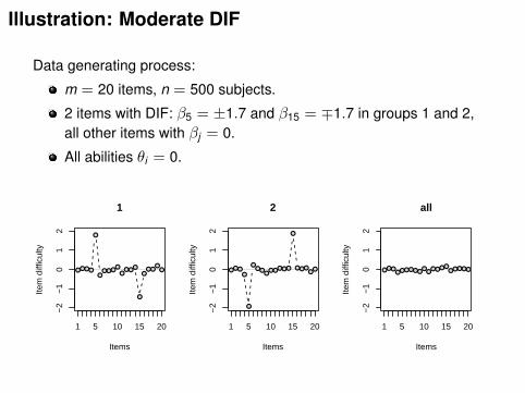
Illustration: Moderate DIF

Data generating process:

m = 20 items, n = 500 subjects.

2 items with DIF: β5 = ±1.7 and β15 = ∓1.7 in groups 1 and 2,all other items with βj = 0.

All abilities θi = 0.

1

Items

Item

diff

icul

ty

−2

−1

01

2

●●●●

●

●●●●

●

●●●●

●

●●●

●●●●●●

●

●●●●

●

●●●●

●

●●●

●●

1 5 10 15 20

2

Items

Item

diff

icul

ty

−2

−1

01

2

●●●●

●

●●●

●●●●●●

●

●●●●

●●●●●

●

●●●

●●●●●●

●

●●●●

●

1 5 10 15 20

all

ItemsIte

m d

iffic

ulty

−2

−1

01

2

●●●●●●●●●

●●

●●●●●●●●●●●●

●●●●●●●

●●●●●

●●●●●

1 5 10 15 20

Illustration: Moderate DIF

●

●

Number of components

BIC

1 2

1396

013

980

1400

014

020

●

●

●

●

saturatedmeanvar

Illustration: No DIF

Data generating process:

m = 20 items, n = 100 subjects.

No DIF: all item difficulties β = 0.

Differences in scores: θi = 1.5 in group 1, θi = −1.5 in group 2.

Scores

Per

cent

of t

otal

0

20

40

60

0 5 10 15 20

1

0 5 10 15 20

2

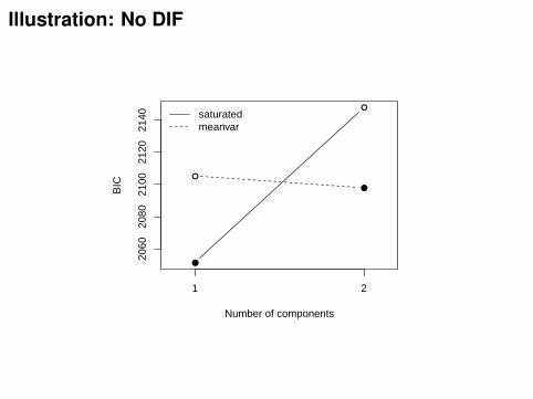
Illustration: No DIF

●

●

Number of components

BIC

1 2

2060

2080

2100

2120

2140

●

●

●

●

saturatedmeanvar

Illustration: No DIF

Items

Cen

tere

d ite

m d

iffic

ulty

par

amet

ers

−2.

0−

1.0

0.0

0.5

●

●

● ●●

● ●

●

●

●

●

●

●

●

●

●

●

● ●

●

●

●

●

●●

●

●

●

● ●● ●

●●

●

●

●

●

●

●

1 5 10 15 20

●

●

Comp. 1Comp. 2

ScoresD

ensi

ty

0 5 10 15 20

0.00

0.10

0.20

0.30

Figure: Estimated item parameters (left) and score probabilities with empiricalscore distribution (right) of the 2-class Rasch mixture model with a meanvarscore specification.

Rasch Mixture Models: Score Probabilities

Goal: Robust specification.

Motivation: When checking for measurement invariance, items are ofinterest, not the scores.

Idea: Useg(r) = constant

Equivalent to: Score distribution is the same over all components.

Interpretation: Score distribution can be multi-modal (if the same overall components).

Open question: What happens if the assumption of equivalence acrosscomponents is violated? Currently under investigation.

Software

Available in R in package psychomix athttp://CRAN.R-project.org/package=psychomix

Based on package flexmix (Grün and Leisch, 2008) for flexibleestimation of mixture models.

Based on package psychotools for estimation of Rasch models.

Frick et al. (2012), provides implementation details and hands-onpractical guidance. See also vignette("raschmix", package

= "psychomix").

Application: Verbal Aggression Data

Behavioral study of psychology students: 243 women and 73 men.Description of frustrating situations:

S1: A bus fails to stop for me.S2: I miss a train because a clerk gave me faulty information.

Behavioral mode: Want or do.

Verbally aggressive response: Curse, scold, or shout.

12 resulting items: S1WantCurse, S1DoCurse, S1WantScold, . . . ,S2WantShout, S2DoShout

Covariates: Gender and an anger score.

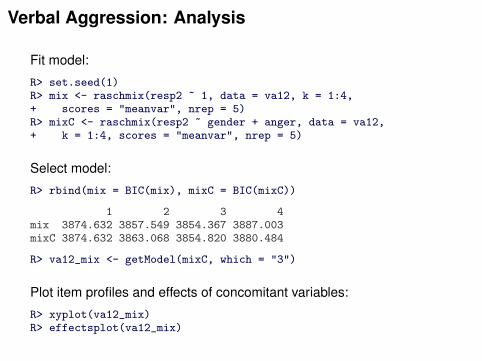
Verbal Aggression: Analysis

Fit model:

R> set.seed(1)R> mix <- raschmix(resp2 ~ 1, data = va12, k = 1:4,+ scores = "meanvar", nrep = 5)R> mixC <- raschmix(resp2 ~ gender + anger, data = va12,+ k = 1:4, scores = "meanvar", nrep = 5)

Select model:

R> rbind(mix = BIC(mix), mixC = BIC(mixC))

1 2 3 4mix 3874.632 3857.549 3854.367 3887.003mixC 3874.632 3863.068 3854.820 3880.484

R> va12_mix <- getModel(mixC, which = "3")

Plot item profiles and effects of concomitant variables:

R> xyplot(va12_mix)R> effectsplot(va12_mix)

Verbal Aggression: Item Profiles

Item

Cen

tere

d ite

m d

iffic

ulty

par

amet

ers

−2

0

2

4

1 2 3 4 5 6 7 8 9 10 11 12

●

●

●

●

●

●

●

●

●

●

●

●

Comp. 1

1 2 3 4 5 6 7 8 9 10 11 12

●

●

● ●

●

●

●

●

●

●

●

●

Comp. 2

1 2 3 4 5 6 7 8 9 10 11 12

●

●

●

●

●

●

●

●

●

●

●

●

Comp. 3

Figure: Item difficulty profiles for the 3-component Rasch mixture model.Items 1–6: Situation S1 (bus). Items 7–12: Situation S2 (train).Order: want/do curse, want/do scold, want/do shout.

Verbal Aggression: Effects Displays

gender effect plot

gender

Com

pone

nt (

prob

abili

ty)

0.2

0.3

0.4

0.5

female male

●

●

Component123

●

anger effect plot

anger

Com

pone

nt (

prob

abili

ty)

0.1

0.2

0.3

0.4

0.5

0.6

10 15 20 25 30 35

Component123

Verbal Aggression: Summary

Number of components: 3 different sets of item parametersnecessary.

Relationship between items differs between the latent classes.

For shouting: Want is less extreme than do. For cursing andscolding, this depends on the latent class.

One class does not differentiate much between the items, for thetwo other classes, cursing/scolding/shouting is increasinglyextreme.

Some dependence on covariates gender and anger score (albeitslightly poorer BIC).

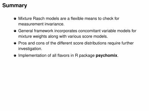
Summary

Mixture Rasch models are a flexible means to check formeasurement invariance.

General framework incorporates concomitant variable models formixture weights along with various score models.

Pros and cons of the different score distributions require furtherinvestigation.

Implementation of all flavors in R package psychomix.

References

Frick H, Strobl C, Leisch F, Zeileis A (2012). “Flexible Rasch Mixture Modelswith Package psychomix.” Journal of Statistical Software, 48(7), 1–25.http://www.jstatsoft.org/v48/i07/

Fischer GH, Molenaar IW (eds.) (1995). Rasch Models: Foundations, RecentDevelopments, and Applications. Springer-Verlag, New York.

Grün B, Leisch F (2008). "FlexMix Version 2: Finite Mixtures with ConcomitantVariables and Varying and Constant Parameters." Journal of StatisticalSoftware, 28(4), 1–35. http://www.jstatsoft.org/v28/i04/

Rost J (1990). “Rasch Models in Latent Classes: An Integration of TwoApproaches to Item Analysis.” Applied Psychological Measurement, 14(3),271–282.