Mixing Of Rubber - ccsuniversity.ac.in · Mixing as a general operation may be considered as three basic processes occurring simultaneously. Simple mixing ensures that the mixture

Mixing Of Rubber

John F. Funt

Mixing of Rubber

John F. Funt

Smithers Rapra Technology Limited

Shawbury, Shrewsbury, Shropshire, SY4 4NR, United KingdomTelephone: +44 (0)1939 250383 Fax: +44 (0)1939 251118

http://www.rapra.net

AuthorAuthor

First Published in 1977 by

Rapra Technology Limited Shawbury, Shrewsbury, Shropshire, SY4 4NR, UK

©2009, Smithers Rapra Technology Limited

All rights reserved. Except as permitted under current legislation no partof this publication may be photocopied, reproduced or distributed in anyform or by any means or stored in a database or retrieval system, without

the prior permission from the copyright holder.

A catalogue record for this book is available from the British Library.

Every effort has been made to contact copyright holders of any material reproduced within the text and the authors and publishers apologise if any have been overlooked.

Typeset by S A Hall Typesetting & DesignPrinted and bound by Lightning Source UK Ltd

Softback ISBN: 978-1-84735-428-0Hardback ISBN: 978-1-84735-150-0

ebook ISBN: 978-1-84735-151-7

3

Acknowledgements

AuthorAuthor

First and foremost I wish to thank Dr. John Jepson and his colleagues in the Research & Development Division of Acushnet Company whose generous support and faith in the application of analysis to industrial processes has made this work feasible. As with all books such as this, the success of the project hinges on the tireless support of a good, competent secretary and typist. Susan Hartman has performed a yeoman task with rare skill and good humour.

Finally, Professor J.R.A. Pearson has served me well as a sounding board for the development of arguments. As a colleague he has been a delight and as a teacher he has been an inspiration.

4

Mixing of Rubber

Contents

i

Contents

Acknowledgements

1. Introduction ................................................................................................1

2. Blending of Particles ....................................................................................5

2.1 The Statistical Description of Mixing .................................................5

2.1.1 Confi dence Limits ....................................................................9

a. Confi dence Limits for the Mean ........................................ 9b. Confi dence Limits for the Variance ................................... 10

2.1.2 Signifi cance Tests ...................................................................10

a. Signifi cance of the Mean Test (Student’s t-Test) ................ 10b. Signifi cance of the Variance (F-test) .................................. 11c. Signifi cance of the Distribution (�2-test). .......................... 11EXAMPLE 1: Confi dence of the Mean Test ......................... 12EXAMPLE 2: Confi dence of the Variance Test ..................... 13EXAMPLE 3: Signifi cance of the Mean Test ......................... 14EXAMPLE 4: Signifi cance of the Distribution Test ............... 14EXAMPLE 5: Calculation of Blending Ratios ...................... 15

2.2 Defi nitions of Mixedness ...................................................................15

2.3 The Kinetics of Simple Mixing ..........................................................18

EXAMPLE 6: Kinetics of Tumble Blending .......................... 23EXAMPLE 7: Calculation of Blending Effi ciency ................. 24

2.4 Multicomponent Mixtures and Markov Chains ................................24

2.5 Mixing Equipment ............................................................................30

2.5.1 Tumble Blenders .......................................................................30

2.5.2 Blade Mixers ............................................................................33

2.5.3 Air and Gravity Feed Mixers ....................................................36

2.5.4 Equipment Selection .................................................................40

AuthorAuthor

Mixing of Rubber

ii

2.6 Summary ...........................................................................................40

References ..................................................................................................41

3. Laminar and Dispersive Mixing .................................................................43

3.1 Laminar Shear Mixing .......................................................................43

3.1.1 Calculation of Striation Thickness .........................................45

3.1.2 The Effect of Streamline Orientation .....................................50

3.2 Dispersive Mixing .............................................................................52

3.2.1 Calculation of forces on a particle .........................................53

3.2.2 Flow in Thin Channels ..........................................................56

3.2.3 The Kinetics of Particle Dispersion ........................................60

3.3 Masterbatches ...................................................................................62

3.4 Incorporation of Carbon Black ..........................................................65

3.5 Summary ...........................................................................................67

References ..................................................................................................67

4. The Milling of Rubbers .............................................................................69

4.1 The Analysis of a Calendar ................................................................70

4.1.1 Basic Flow Equations ............................................................71

4.1.2 Power-law Fluids ...................................................................80

4.1.3 Scaling Laws ..........................................................................84

4.2 Processing Instabilities .......................................................................89

4.3 Heat Transfer ....................................................................................96

4.4 Scale-up Alternatives .........................................................................99

4.5 Commercial Mills ............................................................................104

4.6 Summary .........................................................................................105

References ................................................................................................105

5. Internal Mixers ........................................................................................107

5.1 Flow in an Internal Mixer ...............................................................107

Contents

iii

5.2 Analysis of an Internal Mixer ..........................................................112

5.3 Alternative Mixer Models ...............................................................119

5.4 Heat Transfer in Internal Mixers .....................................................126

5.5 The Effect of Ram Pressure .............................................................131

5.6 Commercial Internal Mixers ............................................................134

5.7 Scaling Laws and Dump Criteria for Internal Mixers .....................137

5.7.1 Geometric Similarity ............................................................139

5.7.2 Maximum Shear Stress ........................................................142

5.7.3 Total Shear Strain ................................................................145

5.7.4 Work Input ..........................................................................148

5.7.5 Constant Mixing Time ........................................................153

5.7.6 Constant Stock Temperature ...............................................154

5.7.7 Constant Weissenberg and Deborah Numbers .....................155

5.7.8 Graetz and Griffi ths Numbers .............................................156

5.8 Summary .........................................................................................158

References ................................................................................................158

6. Continuous Mixers ..................................................................................161

6.1 Mixing in Single Screw Extruders ....................................................161

6.1.1 Mathematical Formulation ..................................................162

6.1.2 Non-Standard Geometry .....................................................169

6.2 Mixing in Two-Screw Extruders ......................................................173

6.3 Summary .........................................................................................175

References ................................................................................................175

7. Powdered Rubbers ...................................................................................177

7.1 Preparation ......................................................................................177

7.1.1 Mechanical Pulverisation (Grinding) ...................................177

7.1.2 Spray Drying .......................................................................177

7.1.3 Coagulation.........................................................................178

Mixing of Rubber

iv

7.2 Mixing Powdered Rubbers ..............................................................178

7.3 The Infl uence of Particle Morphology .............................................179

7.4 Evaluation of Powdered Rubbers ....................................................179

EXAMPLE 1: Potential Unit Savings for Powder Rubber ... 181

References ................................................................................................181

1

Introduction

Since the discovery of vulcanization in the nineteenth century, rubber has been a major industrial product. From its inception, the use of vulcanising agents, reinforcing fi llers and other additives has been a major feature of the rubber industry. Innumerable articles and texts attest to the skill in balancing the chemical and physical properties of the manufactured products.

In most cases, experimenters have been concerned with how recipe changes affect the product properties while the physical processes which formed the test specimen are not considered. For the rubber processor, however, it is these mechanical operations which form the heart of his business. The equipment needed for plant-scale production requires millions of dollars of capital investment. In the highly competitive rubber industry, the ability to save two or three cents per pound of product through better design or more effi cient operation of mixing equipment can make a tremendous difference in the profi tability of a company. Despite the commercial importance of the process, no comprehensive analysis of rubber mixing, considered as a unit operation, is currently available. This monograph is designed to fi ll that gap in the arsenal available for problem solving by the production engineer or the machine designer.

Mixing as a general operation may be considered as three basic processes occurring simultaneously. Simple mixing ensures that the mixture has a uniform composition throughout its bulk, at least when viewed on a scale large compared to the size of the individual particles. In the case of solids blending (Chapter 2), the particle size need not change, but the distribution of particles throughout the mixture approaches a random distribution.

If the shear forces are suffi ciently large, particles may fracture, as in dispersive mixing, and the polymer may fl ow, as in mixing (Chapter 3). In both of these processes, the size of the original particles or fl uid elements changes because of the mixing process. Then the properties of the mixture depend upon the size of the basic structures reached during mixing. In the case of laminar mixing, the size may be the striation thickness of a hypothetical fl uid element, which is inversely related to the total shear strain. If relatively strong particles, or aggregates of particles, are present, these must be reduced in size by the action of forces generated by fl ow in the mixer. Then the size is the actual additive particle size.

Introduction

AuthorAuthor 1

2

Mixing of Rubber

The relative balance between the importance of these three processes in determining the effi ciency of mixing and the product quality depends upon the attraction between particles, the rubber fl ow properties, the geometry of the mixer and the operating conditions such as temperature, mixing time and rotor speed.

The interaction of operating conditions, raw material properties and the quality of mixing can be a formidable phenomenon to analyse. However, in many cases a number of simplifying assumptions about the operation can be made. The fi rst of these is that in any piece of mixing equipment, there is one vital section where the fl ow conditions in that region determine the rate and quality of mixing; the essential physical processes can be described if fl ow in that region can be analysed. For two roll-mills (Chapter 4) this is the nip region; it is the region between the rotor tip and chamber wall for internal mixers (Chapter 5). In every case, the geometry of the mixer is treated locally as if it were fl ow between parallel planes and the actual mixer geometry is incorporated by allowing the space between these hypothetical planes to vary with position in the mixer; this is the basis of the lubrication approximation.

For most mixing operations, the primary driving force for fl uid motion is drag fl ow caused by the relative options of metal boundaries in the equipment. Pressure fl ow is relatively unimportant for mixing. In many cases, the rubber can be treated as Newtonian or a power-law fl uid, which greatly simplifi es the analysis. However, the visco-elastic nature of rubber compounds imposes a severe limitation on the stability of the mixing operation (Chapter 4).

One major limitation to the speed of operation of a mixing process, besides the mechanical ruggedness of the equipment, is the temperature rise in the rubber stock because of viscous dissipation. The heat transfer in mixing equipment may be a problem, especially in larger mixers. The effi ciency of heat transfer depends upon the geometry of the mixer and the operation conditions, as treated in the analyses.

Following a basic description of the three fundamental processes it is necessary to see how these occur in actual mixers. The primary difference between types of mixers is the geometry of the metal boundaries. In two-roll mills (Chapter 4) the geometry is the simple symmetry of parallel cylinders. With internal mixers (Chapter 5) and continuous mixers (Chapter 6) the geometry is more complex. Yet the same kind of fl uid mechanical analysis can be used for all types of mixers.

One of the most common problems facing a process engineer is how to transfer a product from a small laboratory mixer to a plant scale machine. Simple rules for scale-up can be extracted from the analyses of each mixer type based upon an understanding of the fundamental processes. These are treated in some detail for each mixer because of their importance in handling processing problems. Although the terminology used is that for scale-up, the same rules can easily be used for process control to reduce batch-to-batch variability. Essentially the rules tell how to set the operating variables for a mixer when

3

Introduction

the required conditions for good mixing of a material on the same or a different mixer are known.

The basic fl ow equations can also be used in their complete form for the model calculations on a computer to study basic mixer performance.

In the chapters that follow, a description of the basic fl ow processes is fi rst developed. Then these are applied to commercially important mixers to obtain a quantitative description of their operation. These analyses form the basis of a rational, coherent description of rubber mixing which can be used for machine design, process control and process scale-up.

4

Mixing of Rubber

5

Blending of Particles


AuthorAuthor 2The blending of particulate solids without a phase change involves the spatial rearrangement of the particles without a change in particle size. A random distribution of the particles is usually sought and expected so that the concepts of probability and statistics can be used to describe the process. In this chapter quantitative methods for calculating the state of the mixture will be described followed by a discussion of the kinetics of mixing and the effi ciency of mixer designs.

2.1 The Statistical Description of Mixing

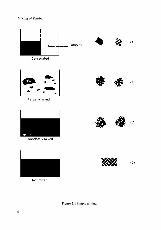
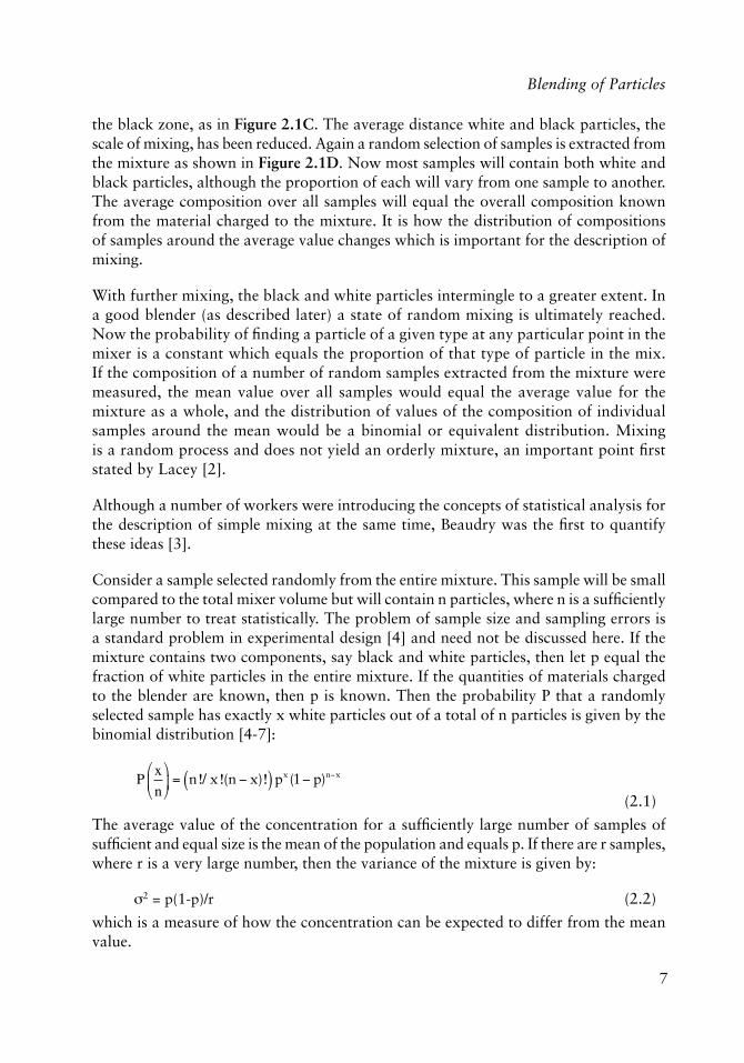
The quantitative evaluation of the state of a mixture, its degree of mixing and the kinetics of mixing is given by the statistical theory of mixing. Simple mixing, the process achieved by blending, can be understood by considering Figure 2.1. Initially the entire contents of the mixer or blender is partitioned into two sections, one of which contains only white particles and the other contains only black particles. Each particle is very small compared to the size of the apparatus and there is a large but fi nite number of each kind of particle. Consider then that a number of small samples are extracted from the apparatus from randomly selected positions in the mixture. Each sample thus selected will be large enough to contain a suffi cient number of particles to treat using statistical methods but will be small enough to leave the mixture essentially unchanged. These requirements on sample selection can pose experimental problems for a practical application, but for the idealised mixture considered here, the conditions can be considered to be met. Several representative samples taken from the mixture, as suggested in Figure 2.1A are shown enlarged in Figure 2.1B. The scale of mixing is the average distance separating one type of particle from a different type of particle [1]. Before the process commences, the scale of mixing in this example is larger than a sample size, Figure 2.1B, and is of the same order as the dimensions of the equipment. Except for a few samples which might be selected from the interface separating the two mixer regions, a sample from the starting material will contain either all white particles or all black particles.

At a later time after the mixing process has begun, some black particles have moved into the region initially occupied by white particles and some white particles have moved into

6

Mixing of Rubber

Figure 2.1 Simple mixing

7


the black zone, as in Figure 2.1C. The average distance white and black particles, the scale of mixing, has been reduced. Again a random selection of samples is extracted from the mixture as shown in Figure 2.1D. Now most samples will contain both white and black particles, although the proportion of each will vary from one sample to another. The average composition over all samples will equal the overall composition known from the material charged to the mixture. It is how the distribution of compositions of samples around the average value changes which is important for the description of mixing.

With further mixing, the black and white particles intermingle to a greater extent. In a good blender (as described later) a state of random mixing is ultimately reached. Now the probability of fi nding a particle of a given type at any particular point in the mixer is a constant which equals the proportion of that type of particle in the mix. If the composition of a number of random samples extracted from the mixture were measured, the mean value over all samples would equal the average value for the mixture as a whole, and the distribution of values of the composition of individual samples around the mean would be a binomial or equivalent distribution. Mixing is a random process and does not yield an orderly mixture, an important point fi rst stated by Lacey [2].

Although a number of workers were introducing the concepts of statistical analysis for the description of simple mixing at the same time, Beaudry was the fi rst to quantify these ideas [3].

Consider a sample selected randomly from the entire mixture. This sample will be small compared to the total mixer volume but will contain n particles, where n is a suffi ciently large number to treat statistically. The problem of sample size and sampling errors is a standard problem in experimental design [4] and need not be discussed here. If the mixture contains two components, say black and white particles, then let p equal the fraction of white particles in the entire mixture. If the quantities of materials charged to the blender are known, then p is known. Then the probability P that a randomly selected sample has exactly x white particles out of a total of n particles is given by the binomial distribution [4-7]:

P

x

n

�

��

�

�� = n!/ x!(n x)!( ) px (1 p)nx

(2.1)

The average value of the concentration for a suffi ciently large number of samples of suffi cient and equal size is the mean of the population and equals p. If there are r samples, where r is a very large number, then the variance of the mixture is given by:

2 = p(1-p)/r (2.2)

which is a measure of how the concentration can be expected to differ from the mean value.

8

Mixing of Rubber

Because only whole particles are in the sample, the measured values of concentration can only assume discrete values. The binomial distribution is a discrete-valued function and can therefore properly describe the sample composition. However, with the large number of sample particles, calculations using a discrete function can become tedious. If the conditions:

p < 0.5 (2.3)

and

rp > 5 (2.4)

are met, which defi ne what is meant by a suffi ciently large number of samples, then the distribution can be treated as continuous to a good approximation and the Gaussian distribution results:

fx

n

�

��

�� =

1

� 2�( )1/2exp �1 / 2

xn� p

�

��

�

��

2

/ �2�

��

�

��

(2.5)

where f is the probability that a sample has composition x/n. If the fraction of the component of interest p is small, then a better approximation to the binomial distribution is given by the Poisson distribution [4, 5]:

f

xn

�

��

�

�� = emmx / x!

(2.6)

where m = np.

In practice, a limited number of samples, each with a different number of particles, is counted. Then if r is the number of samples measured, the mean value of the sample concentration can be calculated:

xn

�

��

�

�� =

xn

�

��

�

��

i=1

r

�i

/ r

(2.7)

where (x/n)i is the measured particle fraction of the component of interest in sample i. the variance of the sample can be calculated:

s2 =xn

�

��

��

i

�xn

�

��

�

��

�

��

�

��

2

/ r �1( )i=1

r

(2.8)

or equivalently:

9


s2 = rxn

�

�

�

��

2

�xn

�

�

�

��

ii=1

r

��

�

�

��

2

i=1

r

��

�

��

��/ r �1( )

(2.9)

The calculated values of the sample mean and variance can be used in two ways. As will be discussed in Section 2.2, the variance can be used to characterise the state of mixing for kinetic calculations. But fi rst, this information can be used to answer the important question of how closely do the samples represent the mixture as a whole. The concentrations in individual samples would be expected to vary because of the random nature of the mixture, because of random sampling errors and because of random errors in measurement. The actual mean and variance of the population as a whole, that is the entire mixture, are unknown so some estimate must be made as to whether or not the measured values are those expected from samples taken from a random mixture. Statistical tests using confi dence limits are used for this purpose. A related problem is to decide whether or not two mixtures with different measured values of the mean and variance can be considered to the same or different, for which purpose signifi cance tests may be used.

2.1.1 Confi dence Limits

Confi dence limits express quantitatively the percentage of times the true but unknown values of the population mean or variance, that is the values of the complete mixture, will lie within a range of values based upon estimates made from a limited number of sample measurements. For example, using the Student’s t-Test described below, the measured value of the average sample composition can be used to make a statement such as ‘nineteen times out of twenty, the true mean composition of the batch will be between 26% and 32% carbon black’. Information of this type is used for calculations in processes downstream from the blending operation where there may be a limit on the maximum, minimum or range of compositions which will yield a satisfactory product.

a. Confi dence Limits for the Mean

From the mean and variance calculated for r samples from Equations (2.7), (2.8) and (2.9), the confi dence limits of the population mean are calculated:

p =

xn

�

��

�

��± ts / r1/2

(2.10)

where p is the population mean. Values of t are tabulated in standard references [4, 8]. For the desired confi dence limits, usually 95% certainty, the value of t for the r-1 degrees of freedom are found in the appropriate table and substituted into equation (2.10), as shown in Example 1.

10

Mixing of Rubber

b. Confi dence Limits for the Variance

Chi-squared (x2) tables [4, 8] are used to calculate the confi dence limits for the population variance in a similar manner. For r-1 degrees of freedom, two values are found in the table. First the value x1

2 is found which is so small that anything less than that would occur less than 2.5% of the time. Secondly, the value x2

2 is found which is so large that any value greater than that will occur less than 2.5% of the time. These correspond to probabilities P = 0.025 and 0.975, respectively. Then the chi-squared values will be within these limits 95% of the time and the population variance can be estimated:

rs2

x22

< �2 <rs2

x12

(2.11)

as shown in Example 2. In addition to placing limits on the values of the mean and variance of the mixture as a whole, confi dence limits test can be used to describe blender effi ciency as presented in a later section.

2.1.2 Signifi cance Tests

Signifi cance tests express quantitatively whether or not the set of samples has the same characteristics as some reference material. This reference material may be the composition required for processing downstream for quality control purposes in preparing new batches. The reference material may be a hypothetical perfectly random mixture having the same overall composition as the sample, or the reference material may be a laboratory-mixed sample when scaling large-size equipment.

Each of the signifi cance tests is a ‘null hypothesis’ test. First it is postulated that the reference and the sample material have exactly the same composition. Then a parameter is calculated based on the values of the mean and variance of the sample and on the known values of the reference. The calculated parameter is compared to tabulated values for the desired level of signifi cance. If the values of the parameter are within prescribed limits, the difference in values of the mean or variance from sample to reference cannot be considered statistically signifi cant.

a. Signifi cance of the Mean Test (Student’s t-Test)

The sample mean and variance are calculated using Equations (2.7) and (2.8) or (2.9). Rearranging Equation (2.10), the value of t may be calculated:

11


t =

xx

�

��

�

�� m

s / r1/2

(2.12)

where m is the mean value of the reference material. The calculated value of t is compared to tabulated values corresponding to r-1 degrees of freedom and the desired level of signifi cance, which is usually 5%. The calculated t will exceed the tabulated value by chance only 5% of the time if the reference and sample mixtures are the same (Example 3).

b. Signifi cance of the Variance (F-test)

The variance of the reference material sr2 and the sample material ss

2 are calculated using Equations (2.8) or (2.9), and the F value is calculated:

F = ss

2 / sr2

(2.13)

Tabulated values of F will determine if this large a value of F can occur by chance alone with the required degree of signifi cance if the two batches are the same.

c. Signifi cance of the Distribution (�2-test).

In this calculation, let mi be the measured frequency that a value (x/n)i is observed in a set of random samples. The expected value of the frequency for a randomly mixed material fi is given by Equations (2.1), (2.5) or (2.6). Then the chi-square value can be calculated:

�2 = mi � fi( )2 / fi

i=1

k

� (2.14)

where k is the number of pairs of observed and expected frequencies. The calculated chi-square value can be compared to tabulated values for k-l degrees of freedom to determine if the differences in distributions of values can occur by chance at the desired level of statistical signifi cance (Example 4).

The use of these types of tests in a blending problem involving a master batch is shown in Example 5.

Although the statistical calculations are simple to perform, they often become tedious, especially in quality control work where rapid answers are often needed from semi-skilled operators. Especially in the case of powder blending treated in this chapter where

12

Mixing of Rubber

later operations can smooth fl uctuations by back-mixing, a simpler method is available. A relative frequency histogram of the standard batch can be prepared on an acetate transparency. The histogram of new batches can be plotted on graph paper to the same scale by the quality control operator. An overlay of the transparency will quickly show if there are signifi cant differences between the sample and the standard.

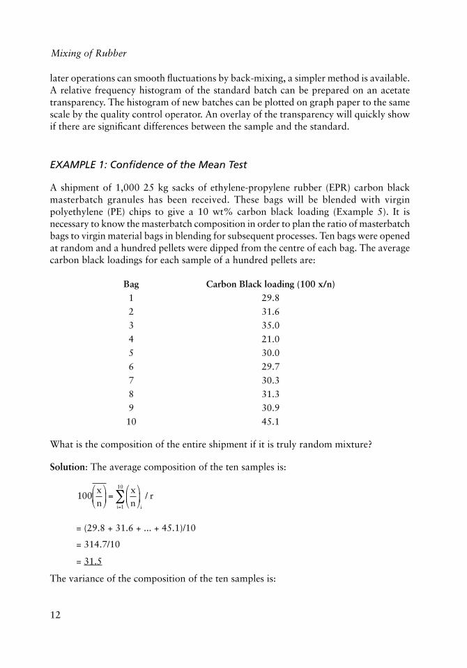
EXAMPLE 1: Confi dence of the Mean Test

A shipment of 1,000 25 kg sacks of ethylene-propylene rubber (EPR) carbon black masterbatch granules has been received. These bags will be blended with virgin polyethylene (PE) chips to give a 10 wt% carbon black loading (Example 5). It is necessary to know the masterbatch composition in order to plan the ratio of masterbatch bags to virgin material bags in blending for subsequent processes. Ten bags were opened at random and a hundred pellets were dipped from the centre of each bag. The average carbon black loadings for each sample of a hundred pellets are:

Bag Carbon Black loading (100 x/n)1 29.8

2 31.6

3 35.0

4 21.0

5 30.0

6 29.7

7 30.3

8 31.3

9 30.9

10 45.1

What is the composition of the entire shipment if it is truly random mixture?

Solution: The average composition of the ten samples is:

100

xn

�

��

�

�� =

xn

�

��

�

��

i

/ ri=1

10

�

= (29.8 + 31.6 + ... + 45.1)/10

= 314.7/10

= 31.5

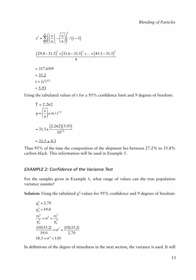
The variance of the composition of the ten samples is:

13


s2 =xn

�

��

�

i

�xn

�

��

�

�

�

��

�

�

2

/ r �1( )i=1

10

�

29.8 31.5( )2+ 31.6 31.5( )2

+…+ 45.131.5( )2

9

= 317.69/9

= 35.2

s = (s2)1/2

= 5.93

Using the tabulated values of t for a 95% confi dence limit and 9 degrees of freedom:

T = 2.262

p =

xn

�

��

�

��± ts / r1/2

= 31.5±

2.262( ) 5.93( )101/2

= 31.5 ± 4.3

Thus 95% of the time the composition of the shipment lies between 27.2% to 35.8% carbon black. This information will be used in Example 5.

EXAMPLE 2: Confi dence of the Variance Test

For the samples given in Example 1, what range of values can the true population variance assume?

Solution: Using the tabulated �2-values for 95% confi dence and 9 degrees of freedom:

�12 = 2.70

�22 = 19.0

rs2

�22

< �2 <rs2

�12

(10)(35.2)19.0

< �2 <(10)(35.2)

2.7018.5 < �2 < 130

In defi nitions of the degree of mixedness in the next section, the variance is used. It will

14

Mixing of Rubber

be necessary to decide whether changes in the value of the variance will be due to the random nature of a mixture or whether the changes are caused by a change in the state of the mixture. The range of population variance calculated here will aid in that analysis.

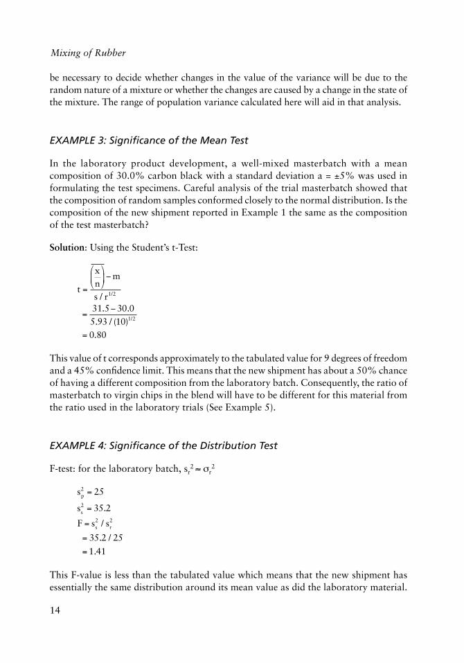
EXAMPLE 3: Signifi cance of the Mean Test

In the laboratory product development, a well-mixed masterbatch with a mean composition of 30.0% carbon black with a standard deviation a = ±5% was used in formulating the test specimens. Careful analysis of the trial masterbatch showed that the composition of random samples conformed closely to the normal distribution. Is the composition of the new shipment reported in Example 1 the same as the composition of the test masterbatch?

Solution: Using the Student’s t-Test:

t =

xn

�

��

�

�� m

s / r1/2

=31.5 30.05.93 / (10)1/2

= 0.80

This value of t corresponds approximately to the tabulated value for 9 degrees of freedom and a 45% confi dence limit. This means that the new shipment has about a 50% chance of having a different composition from the laboratory batch. Consequently, the ratio of masterbatch to virgin chips in the blend will have to be different for this material from the ratio used in the laboratory trials (See Example 5).

EXAMPLE 4: Signifi cance of the Distribution Test

F-test: for the laboratory batch, sr2 � r

2

sp2 = 25

ss2 = 35.2

F = ss2 / sr

2

= 35.2 / 25

= 1.41

This F-value is less than the tabulated value which means that the new shipment has essentially the same distribution around its mean value as did the laboratory material.

15


EXAMPLE 5: Calculation of Blending Ratios

In addition to quality control applications in Examples 3 and 5, the statistical description of the masterbatch shipment is used in product formulation. The masterbatch shipment described in Example 1 is to be blended with virgin PE chips to give a 10 wt% carbon black loading. Because of contractual specifi cations with the customer, there must be at least 10% carbon black in 97.5% of the blended samples. The problem is to calculate the proportion of masterbatch required.

Solution: Let

M = weight fraction of masterbatch (MB)

P = weight fraction of carbon black in MB

=

xn

�

��

�

��± ts / r1/2

pM = weight fraction of carbon black in blend

M(p-(ts/r1/2)) = 0.10

0.272M = 0.10

M = 0.10/0.272

= 0.36

If the concentration in the masterbatch was uniformly equal to the average:

M = 0.10/0.315

= 0.32

If the mean concentration in the shipment was the same as in the laboratory tests:

M = 0.10/0.257

= 0.39

Thus the uncertainty in the concentration of the shipment means that 12% more masterbatch must be used than would be the case if the concentration was uniform. However, because the new shipment has a higher average carbon black loading than the laboratory material, approximately 7% less masterbatch is required than in the trials.

2.2 Defi nitions of Mixedness

Some of the earliest attempts to quantify the degree of mixing were made in the 1930s by Oyami [7, 9]. After attempts to rationalise empirical data on the kinetics of powder blending by qualitative appeals to statistical ideas [10, 11], the concept of the degree of

16

Mixing of Rubber

mixing was put on a fi rm quantitative base by Beaudry [3]. Essentially all subsequent defi nitions have been based on a combination of Oyama’s and Beaudry’s concepts.

Oyama measured the spatial variation of light absorption across the face of a cylinder containing clear and black particles [7]. The maximum differences in absorption between any two locations at the beginning of the test and after various mixing times were measured. Then the degree of mixing (DM) was defi ned by:

DM = 1�

�i max, t�i max,0

(2.15)

where �imax is the maximum difference in light absorption measured at times t and 0 . The idea of expressing the degree of mixing as a linear function of some measured or calculated property of the mixture has been used by most subsequent authors.

Beaudry [3] was the fi rst to use the quantitative results of the statistics of random sampling to describe blending. The variance among batches before blending sb

2 and after blending sx

2 were calculated using a variation of Equation (2.9):

s2 =

Ci2�

r�C2

(2.16)

Where Ci is the value of the measured property (particle count, colour, composition, etc.) of the ith batch and c is the average value for all batches. The value of the variance for a theoretically perfectly random mixture sp

2 was calculated from the normal distribution having the same overall average composition. Then the limited blending ratio � is calculated:

� = sb

2 / sp2

(2.17)

and the blending effi ciency (BE) for any operation is calculated:

BE =

sb2

sx2

�

��

�

��actual1

� 1�100%

(2.18)

This can be seen to be an extension of Oyama’s linear function principle where the statistical distribution of a measured property is used rather than the property itself.

Lacey [2] initially used the standard deviation of the samples as a measure of mixedness:

DM = s = p 1 p( ) / n( )1/2

(2.19)

17


where p is the average composition of n samples. Later he suggested a linear function of the variance [12]:

DM =

so2 s2

so2 sr

2

(2.20)

where so2 is the theoretical variance for a completely unmixed material, so

2 = p(1-p), and sr

2 is the theoretical variance for perfect mixing, sr2 = p(1-p)/n, where the composition p

is known from the amounts of materials charged and the sample variance s2 is calculated from the measured samples. It can readily be seen that the defi nition of the degree of mixing is essentially the same as the blending effi ciency defi ned by Beaudry.

Michaels and Puzinowskas [13] defi ned a uniformity index IV:

Iv = Dv / Dvo

(2.21)

where:

Dv = Ci �Cav( )2

/ nCavi=1

n

��

��

�

�

1/2

(2.22)

and

Dvo = 1 Cav( ) / Cav( )1/2

(2.23)

The uniformity index, which is similar to Danckwerts Intensity Factor [1], varies from 1.0 for unmixed materials to 0 for a completely randomly mixed material.

Weidenbaum and Bonilla [14] used chi-squared as a measure of mixedness and assigned qualitative meaning to the relative frequency of �2:

If P(�2) equals Designate mixture as<0.1 Very poor

0.1 – 0.3 Poor0.3 – 0.7 Fair0.7 – 0.9 Good

>0.9 Excellent

They also suggested as an alternative degree of mixing:

DM = /s (2.24)

Where and s are the standard deviations of perfectly mixed material and the actual samples.

18

Mixing of Rubber

Smith [15] used a similar defi nition:

DM = o/s (2.25)

Where:

o = (p(1-p))1/2

Eustik [16] considered the mixing of particles of granular material with a known size distribution and interpreted his results in terms of a standard deviation. Adams and Baker [5] considered the problem of mixing a small amount of masterbatch with large amounts of polymer using a Poisson distribution rather than a Gaussian distribution.

Of the various defi nitions of mixedness, either the variance of the measured property of the material or a linear function of the variance (Equations (2.18) or (2.20)) have proven the most useful, in describing the effi ciency of a mixing operation or the kinetics of mixing.

2.3 The Kinetics of Simple Mixing

In principle any one of the listed criteria of mixedness or the mean or standard deviation of the mixture could be used to establish the kinetics of a mixing operation. The appropriate mixing measure is plotted as a function of the mixing time. The curve is used directly as an evaluation of the kinetics of mixing or it is analysed using a model for the mixing process.

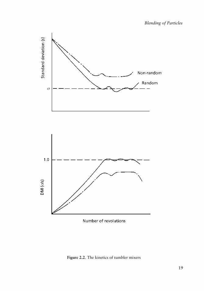
In a study of various tumble blenders, Weidenbaum and Bonilla [14] calculated the standard deviations of samples taken at various mixing times. As shown in Figure 2.2, the sample standard deviation decreased to the value expected for a random sample. At long mixing times, the standard deviation increased because of axial segregation caused by geometrical differences in the particles. Even with the same tumbler and the same particles, the curve in Figure 2.2A would be shifted up or down with a change in the mean concentration which would change the standard deviation of the randomly mixed sample. To overcome this problem, the degree of mixing can be used:

DM = /s (2.24)

In this case, the curve rises asymptotically to a value 1.0 before decreasing again at longer times if the mixture achieves a random distribution. In some cases, the mixing process may not reach a random distribution but the standard deviation will still reach an asymptotic value. This may occur in tumble blending of particles with a large density difference where there may be a tendency to segregate particles vertically by density. In this case, the asymptotic value may be used to normalise the degree of mixing.

For a number of materials and blenders, it was found that the kinetics of mixing could be described by the equation:

19


Figure 2.2. The kinetics of tumbler mixers

20

Mixing of Rubber

d � / s( )dt

= �k�s

�

��

�

��

eq

�s

�

��

�

��

�

��

�

��

(2.26)

where

�s

�

��

�

��

eq = 1.0 for a random mixture. This states that blending is a linear rate process

and k� is a measure of how good a mixer is. Integration of the rate expression yields:

ln1

�

s

�

��

�

��

eq

�

s

�

��

�

��

�

�

��

�

�

��

= ln1

�

s

�

��

�

��

eq

�

s

�

��

�

��

o

�

�

��

�

�

��

+ �k t

(2.27)

For a simple mixing in tumble blenders, the rate of mixing was linear in the degree of mixing.

Earlier Brothman and co-workers [10] considered the surface area separating particles of different types as an appropriate measure of mixing. This could be recast as a probability problem as well.

Let: Sp = maximum surface of separation

yt = fraction of area developed in time t

Zt = 1 – yt

� = measure of the kinetics of mixing.

Then using a fi nite difference formulation for the rate of area generation:

yt+1 = yt + �(1 yt)

(2.28)

This is a fi nite difference formulation of a linear rate expression equivalent to Equation (2.26).

Zt+1 = zt(1 – �) (2.29)

Zt = zo(1 – �)t (2.30)

Zo = 1 – yo � 1 (2.31)

Zt = (1 – �)t (2.32)

1 – yt = (1 – �)t

= etlog(1 – �) (2.33)

yt = 1 – e–tc (2.34)

where:

c = log (1/(1 – �)) (2.35)

21


Then let Ui = probability that a random element has a surface exposed to an interface

Ui = k �Si (2.36)

where:

�S = S/n

S = total interfacial area with n units

Pn = probability that a cubic element has at least one surface exposed to an interface separating two kinds of particles

Pn = 1 – e–ks

= 1 – e–ks p (1 – e–tc) (2.37)

= Pt

If samples are taken at two times, kSp and c can be evaluated and the mixing time required to achieve a desired degree of mixing can be calculated as in Example 6. Then the time required to obtain a desired level of mixing can be calculated:

Pt,E = 1 exp kSp 1 etc( )( )( )

v /vo

(2.38)

where:

vo = sample volume

v = V/x = number of units of volume with at least one particle of minor component

x = number of particles of minor component in volume v

Maitra and Coulson [11] reached the same equations as Brothman et al. using an argument based upon a diffusion analogue.

Beaudry [3] considered the problem of continuous blenders. Considering any property such as the concentration of component A in a mixture which is different between the batches which are to be blended. Then the variance can be used as a measure of mixing.

Let:

vb = variance of property between batches

vx = variance of samples in blender outlet

D = blender volume/batch volume

xo = concentration in blender at start of batch 1

x = concentration in blender at time t

cn = concentration of batch n

22

Mixing of Rubber

Then a balance of component A in the blender yields:

Ddx = c1 dV - x dv (2.39)

for the fi rst batch where:

dv = volume increment

dx = concentration increment

ln

c1 xo

c1 x1

�

��

�

�� =

1D

(2.40)

x1 = (1 – K)c1 + Kxo (2.41)

where:

K = e-1/D

A similar balance for blending the nth batch yields:

xn = (1 – K)cn + Kxn-1

Then the variance can be calculated:

vp = vb(1 – K)2 + vqK2 (2.42)

where:

vp = variance for xn

vq = variance for xn-1

vp =~ vq

vb

vp

=1+ K1 K

(2.43)

If there is fi rst infl ow, then blending, then outfl ow, the expression for K becomes:

K = (D – 1)/D (2.44)

For intermittent infl ow and continuous outfl ow, the expression becomes:

K =

sDsD s 1

�

��

�

��

s/(s1)

(2.45)

where:

s = infl ow rate/outfl ow rate

A blending effi ciency can be defi ned as:

23


BE =vb

vp

�

��

�

��

actual

1�

�

��

�

�

��

100� 1

(2.46)

where:

� =vb

vp

�

��

�

��

ideal

And � is independent of actual blender design. In comparing modes of operation, continuous fl ow gives the best blending; intermittent infl ow and continuous outfl ow is second best, and alternate fl ow gives the least effi cient blending. An example of these equations is given in Example 7.

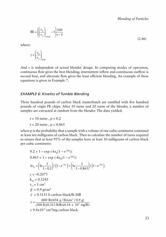
EXAMPLE 6: Kinetics of Tumble Blending

Three hundred pounds of carbon black masterbatch are tumbled with fi ve hundred pounds of virgin PE chips. After 10 turns and 20 turns of the blender, a number of samples are extracted at random from the blender. The data yielded:

t = 10 turns , p = 0.2

t = 20 turns , p = 0.865

where p is the probability that a sample with a volume of one cubic centimetre contained at least ten milligrams of carbon black. Then to calculate the number of turns required to ensure that at least 95% of the samples have at least 10 milligrams of carbon black per cubic centimetre:

0.2 = 1 – exp (-ksp(1 – e-10c))

0.865 = 1 – exp (–ksp(1 – e-20c))

ksp = ln

11 0.2

�

��

�

�� / 1 e10c( ) = ln

11 0.865

�

��

�

�� / 1 e20c( )

c = –0.2075

ksp = 0.1245

vo = 1 cm3

p = 0.9 g/cm3

c = 0.3151 b carbon black/lb MB

v =

(800 lb)(454 g / lb)(cm3 / 0.9 g)(300 lb)(0.315 lb/lb)(4.54 � 105 mg/lb)

= 9.4x10-3 cm3/mg carbon black

24

Mixing of Rubber

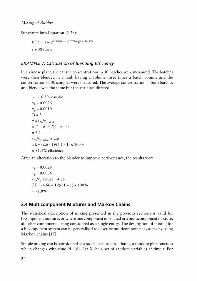
Substitute into Equation (2.38):

0.95 = 1 –(e0.1245(1- exp(.2075t)))(9.4x10-3/1)

t = 38 turns

EXAMPLE 7: Calculation of Blending Effi ciency

In a viscose plant, the caustic concentrations in 30 batches were measured. The batches were then blended in a tank having a volume three times a batch volume and the concentration of 30 samples were measured. The average concentration in both batches and blends was the same but the variance differed:

c = 6.5% caustic

vb = 0.0026

vp = 0.0010

D = 3

� = (vb/vp)ideal

= (1 + e–1/D)/(1 – e–1/D)

= 6.1

(vb/vp)actual = 2.6

BE = (2.6 - 1)/(6.1 - 1) x 100%

= 31.4% effi ciency

After an alteration to the blender to improve performance, the results were:

vb = 0.0028

vp = 0.0006

(vb/vp)actual = 4.66

BE = (4.66 – 1)/(6.1 – 1) x 100%

= 71.8%

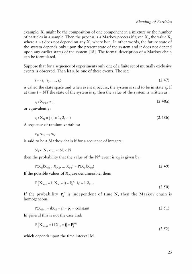
2.4 Multicomponent Mixtures and Markov Chains

The statistical description of mixing presented in the previous sections is valid for bicomponent mixtures or where one component is isolated in a multicomponent mixture, all other components being considered as a single entity. The description of mixing for a bicomponent system can be generalised to describe multicomponent systems by using Markov chains [17].

Simple mixing can be considered as a stochastic process, that is, a random phenomenon which changes with time [4, 18]. Let Xt be a set of random variables at time t. For

25


example, Xt might be the composition of one component in a mixture or the number of particles in a sample. Then the process is a Markov process if given Xt, the value Xa where a > t does not depend on any Xb where b<t . In other words, the future state of the system depends only upon the present state of the system and it does not depend upon any earlier states of the system [18]. The formal description of a Markov chain can be formulated.

Suppose that for a sequence of experiments only one of a fi nite set of mutually exclusive events is observed. Then let sj be one of these events. The set:

s = (s1, s2, ...., sj) (2.47)

is called the state space and when event sj occurs, the system is said to be in state sj. If at time t = NT the state of the system is sj, then the value of the system is written as:

sj : Xt=N� = j (2.48a)

or equivalently:

sj : XN = j (j = 1, 2, ...) (2.48b)

A sequence of random variables:

x1, x2, ..., xN

is said to be a Markov chain if for a sequence of integers:

N1 < N2 < ... < Nr < N

then the probability that the value of the Nth event is xN is given by:

P(XN|XN1 , XN2, ... XNr) = P(XN|XNr) (2.49)

If the possible values of XN are denumerable, then:

P XN+1 = i | XN = j( ) = Pij

(N) i, j = 1,2,… (2.50)

If the probability Pij

(N) is independent of time N, then the Markov chain is homogeneous:

P(XN+1 = i|XN = j) = pij = constant (2.51)

In general this is not the case and:

P XN+M = i | XN = j( ) = Pij

(M)

(2.52)

which depends upon the time interval M.

26

Mixing of Rubber

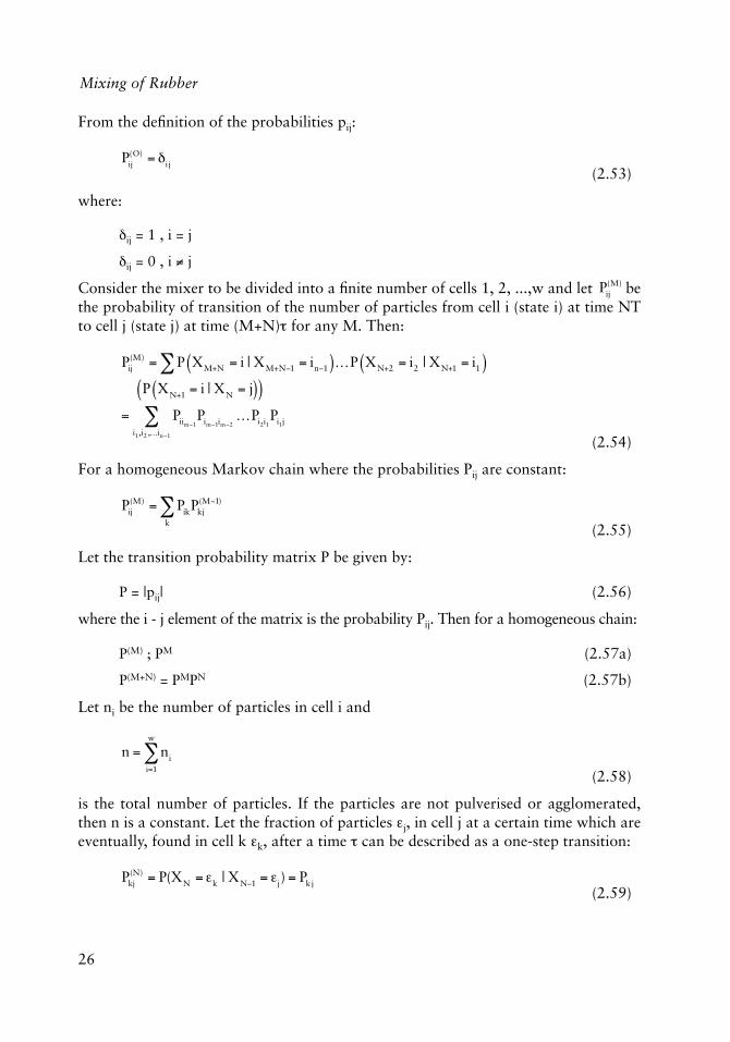
From the defi nition of the probabilities pij:

Pij

(O) = �i j (2.53)

where:

�ij = 1 , i = j

�ij = 0 , i � j

Consider the mixer to be divided into a fi nite number of cells 1, 2, ...,w and let Pij

(M) be the probability of transition of the number of particles from cell i (state i) at time NT to cell j (state j) at time (M+N)� for any M. Then:

Pij(M) = P XM+N = i | XM+N�1 = in�1( )� …P XN+2 = i2 | XN+1 = i1( )

P XN+1 = i | XN = j( )( )= Piim�1

Pim�1im�2…Pi2i1

Pi1ji1,i2 ,…in�1

� (2.54)

For a homogeneous Markov chain where the probabilities Pij are constant:

Pij

(M) = PikPkj(M�1)

k

� (2.55)

Let the transition probability matrix P be given by:

P = |pij| (2.56)

where the i - j element of the matrix is the probability Pij. Then for a homogeneous chain:

P(M) ; PM (2.57a)

P(M+N) = PMPN (2.57b)

Let ni be the number of particles in cell i and

n = ni

i=1

w

� (2.58)

is the total number of particles. If the particles are not pulverised or agglomerated, then n is a constant. Let the fraction of particles �j, in cell j at a certain time which are eventually, found in cell k �k, after a time � can be described as a one-step transition:

Pkj

(N) = P(XN = �k | XN1 = �j) = Pkj (2.59)

27


Pkj = 1 and 0 < Pkj < 1

j=1

w

� (2.60)

This states that even though N steps in the fundamental mixing process may have occurred, it may be treated as a single step in a different time scale. This is particularly important where the process is measured as a function of a variable such as the number of turns in a blender, which may not bear any direct relationship to the basic particle dynamics.

Suppose there is a system containing r components which have identical properties except colour. Let the number of particles of colour j in cell i be mij. Then the total number of particles in cell i is:

ni = mij i = 1,…w

j=1

r

� (2.61)

The total number of j-component particles in the mixer mj is:

mj = mij

i=1

w

� (2.62)

The total number of particles is:

n = ni

i=1

w

� = mjj=1

r

� � mijj=1

r

�i=1

w

� (2.63)

For perfect mixing, the number concentration throughout the mixer will be essentially uniform:

(cj)� = mj/n (2.64)

Let ckj(N) be the concentration of component j in cell k at time t = N�. Then:

lim

N ��ckj(N) = (cj)�

(2.65)

if the mixing is a random process. If the mixing can be described by the fi rst-order Markov process presented above, the number of particles of component i moving from cell j to cell k during time � is given by:

Qj�k(i) = Pkjmji i = 1, ... r; k � j; k,j = 1, ... w (2.66)

Qj�j(i) is the number of particles remaining in cell j and

28

Mixing of Rubber

Qj�j(i) = Pjjmji (2.67)

The fl ow of particles of all components from cell j to k is given by:

Qj�k = Qj�k(i) = Pkj

i=1

r

� mji = Pkji=1

r

� nj

(2.68)

Then:

mij

(N) = Pi�(N)m

�j(0)p=1

w

� (2.69)

where mij

(N) is the number of particles of component j in cell i at time N� after the start of mixing. The number fraction of component j in cell i is:

cij(N) =mij(N)

ni

=1ni

Pij(N)mij(0)

i=1

w

� (2.70)

and

ni = Qj�ij=1

w

�

= Pij(N)nj

j=1

w

� (2.71)

Divide both sides of equation (2.71) by the total number of particles to obtain:

�i = Pij

(N)�jj=1

w

� (2.72)

where �i is the number fraction of particles in cell i and

�i = 1

i=1

w

� (2.73)

Then the particle number balance for component j after N transition steps becomes:

mj = cij(N)ni

i=1

w

� = cij(0)nii=1

w

� = constant

(2.74)

29


Substituting back into Equation (2.70) yields:

cij(N) =

1�i

Pi�(N)�

�c

�j(0)i=1

w

� (2.75)

c

�j (0) = m�j (0) / n

�

(2.76)

In matrix notation, this expression becomes:

C(N) = �-1 P(N) � C(0) (2.77)

Given the initial concentration distribution and the transition matrix, the concentration distribution at any time N� can be calculated. Once the distribution is known, the variance can be calculated:

�N

2 =1r

�i cij(N)� cj�( )2

i=1

w

�j=1

r

� (2.78)

and

cij(N) =

cj�

�i

Pi�(N)q

�j(0)�=1

w

� (2.79)

where:

q

�j(0) = m�j(0) / mj

(2.80)

At the beginning of the mixing process, N = 0 and

�o

2 =1r

(cj�)2

i=1

w

�j=1

r

� �i

1�i

Pi�(N)q

�j(0)�1�=1

w

��

�

��

(2.81)

and a degree of mixing can be defi ned:

DM = 1

�N2

�o2

(2.82)

This result is a generalisation of the equations derived for a bicomponent mixture [19]. Mixing of a bicomponent system can be used to determine the transition probability matrix for a mixing system and these results used to describe multicomponent systems.

30

Mixing of Rubber

2.5 Mixing Equipment

The machinery used to achieve particulate blending can be divided into three classes, depending upon the primary method used to achieve particle motion:

1. Tumble blenders

2. Blade mixers, and

3. Air mixers

In tumble mixers, particle motion is generated by rotating the walls of the container in such a way as to cause layers of particles to tumble over one another under the infl uence of gravity. Blade mixers rely upon positive displacement of the particles by a moving screw or blade combined with random tumbling of the particles. Air mixers rely upon the random motion of particles in a turbulent air stream or in free-fall trajectories in chutes.

2.5.1 Tumble Blenders

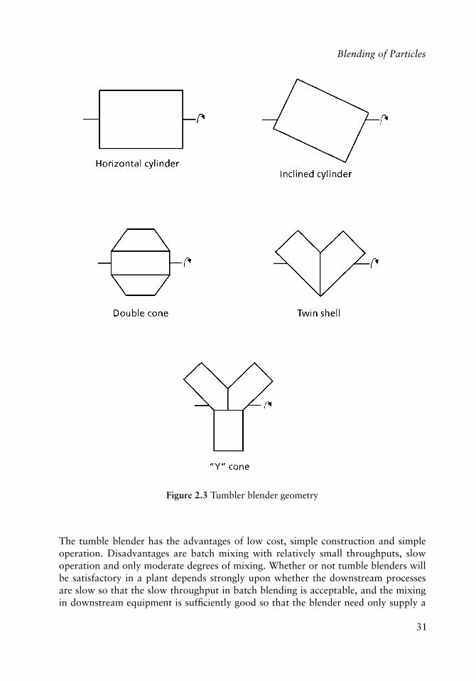
Tumble blenders are the most common mixers used for batch mixing of particulate solids. The main difference among mixers in this class is in the geometry of the mixer. Several common shapes are shown in Figure 2.3.

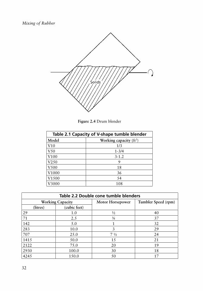
Coulson and Maitra [20] studied tumble blending in a drum mixer shown schematically in Figure 2.4. They found that the best mixing was obtained when the barrel axis was inclined at 14°. Faster mixing was obtained with smaller particles, but segregation (‘unmixing’) was a problem if the particles differed signifi cantly in either size or density. There was an optimum speed of rotation for rapid mixing when all other variables were constant and there was a maximum volume fraction of components in the mixer above which mixing did not occur.

The actual kinetics of mixing depend strongly upon the particle size and shape and the operating conditions. However, the general features have been reported many times. One particular problem in tumble blending, especially with rotation about a horizontal axis of symmetry is that there may be no end-to-end mixing. If there is no horizontal component to the particle velocity in the tumbling, mixing will be poor. Dividing the material as in the twin-shell tumbler was supposed to accomplish this but in general the mixing was poor without internal baffl es [5, 21] . In a comparison of a number of geometries of tumble blenders, Adams and Baker [5] found the best mixing was obtained with a rotating cube. Other geometries gave inferior results.

Tumble blenders are offered by many manufacturers in a wide range of capacities. A typical range is shown in Table 2.1 for a V-shaped blender manufactured by Moritz [22] and in Table 2.2 for a double-cone blender manufactured by Baker Perkins [23].

31


The tumble blender has the advantages of low cost, simple construction and simple operation. Disadvantages are batch mixing with relatively small throughputs, slow operation and only moderate degrees of mixing. Whether or not tumble blenders will be satisfactory in a plant depends strongly upon whether the downstream processes are slow so that the slow throughput in batch blending is acceptable, and the mixing in downstream equipment is suffi ciently good so that the blender need only supply a

Figure 2.3 Tumbler blender geometry

32

Mixing of Rubber

Figure 2.4 Drum blender

Table 2.1 Capacity of V-shape tumble blenderModel Working capacity (ft3)V10 1/3V50 1-3/4V100 3-1.2V250 9V500 18V1000 36V1500 54V3000 108

Table 2.2 Double cone tumble blendersWorking Capacity Motor Horsepower Tumbler Speed (rpm)

(litres) (cubic feet)29 1.0 ½ 4071 2.5 ¾ 37142 5.0 1 32283 10.0 3 29707 25.0 7 ½ 241415 50.0 15 212122 75.0 20 192930 100.0 30 184245 150.0 50 17

33


constant time-average concentration. If the downstream processes cannot eliminate the spatial gradients from a tumble blender, then another method must be used.

2.5.2 Blade Mixers

Blade mixers attempt to overcome the diffi culties inherent in the free motion of tumble blenders by using the positive displacement of a rotating blade. The motion of the blade sweeps particles past one another.

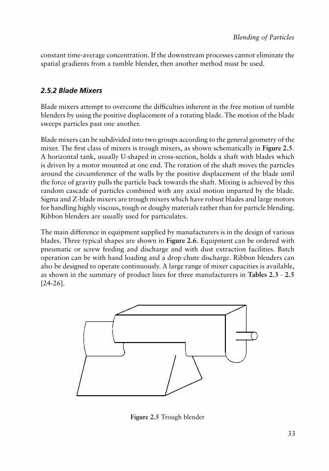
Blade mixers can be subdivided into two groups according to the general geometry of the mixer. The fi rst class of mixers is trough mixers, as shown schematically in Figure 2.5. A horizontal tank, usually U-shaped in cross-section, holds a shaft with blades which is driven by a motor mounted at one end. The rotation of the shaft moves the particles around the circumference of the walls by the positive displacement of the blade until the force of gravity pulls the particle back towards the shaft. Mixing is achieved by this random cascade of particles combined with any axial motion imparted by the blade. Sigma and Z-blade mixers are trough mixers which have robust blades and large motors for handling highly viscous, tough or doughy materials rather than for particle blending. Ribbon blenders are usually used for particulates.

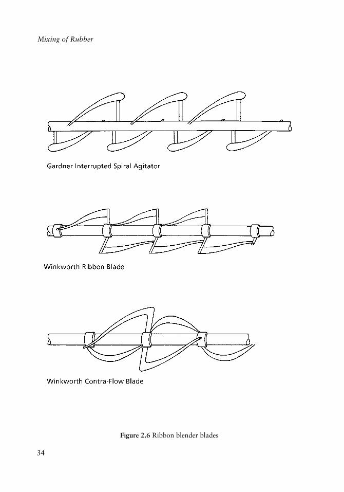
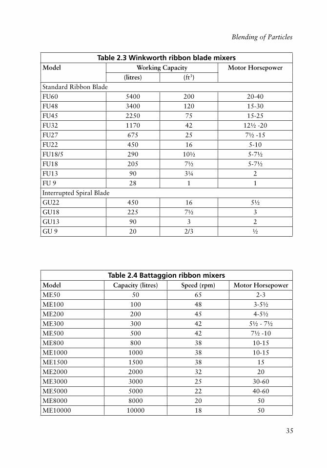
The main difference in equipment supplied by manufacturers is in the design of various blades. Three typical shapes are shown in Figure 2.6. Equipment can be ordered with pneumatic or screw feeding and discharge and with dust extraction facilities. Batch operation can be with hand loading and a drop chute discharge. Ribbon blenders can also be designed to operate continuously. A large range of mixer capacities is available, as shown in the summary of product lines for three manufacturers in Tables 2.3 - 2.5 [24-26].

Figure 2.5 Trough blender

34

Mixing of Rubber

Figure 2.6 Ribbon blender blades

35


Table 2.3 Winkworth ribbon blade mixersModel Working Capacity Motor Horsepower

(litres) (ft3)Standard Ribbon Blade

FU60 5400 200 20-40

FU48 3400 120 15-30

FU45 2250 75 15-25

FU32 1170 42 12½ -20

FU27 675 25 7½ -15

FU22 450 16 5-10

FU18/5 290 10½ 5-7½

FU18 205 7½ 5-7½

FU13 90 3¼ 2

FU 9 28 1 1

Interrupted Spiral Blade

GU22 450 16 5½

GU18 225 7½ 3

GU13 90 3 2

GU 9 20 2/3 ½

Table 2.4 Battaggion ribbon mixersModel Capacity (litres) Speed (rpm) Motor HorsepowerME50 50 65 2-3

ME100 100 48 3-5½

ME200 200 45 4-5½

ME300 300 42 5½ - 7½

ME500 500 42 7½ -10

ME800 800 38 10-15

ME1000 1000 38 10-15

ME1500 1500 38 15

ME2000 2000 32 20

ME3000 3000 25 30-60

ME5000 5000 22 40-60

ME8000 8000 20 50

ME10000 10000 18 50

36

Mixing of Rubber

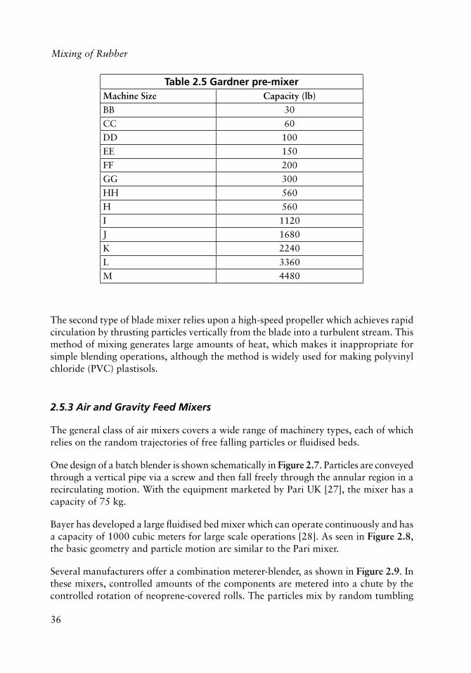
The second type of blade mixer relies upon a high-speed propeller which achieves rapid circulation by thrusting particles vertically from the blade into a turbulent stream. This method of mixing generates large amounts of heat, which makes it inappropriate for simple blending operations, although the method is widely used for making polyvinyl chloride (PVC) plastisols.

2.5.3 Air and Gravity Feed Mixers

The general class of air mixers covers a wide range of machinery types, each of which relies on the random trajectories of free falling particles or fl uidised beds.

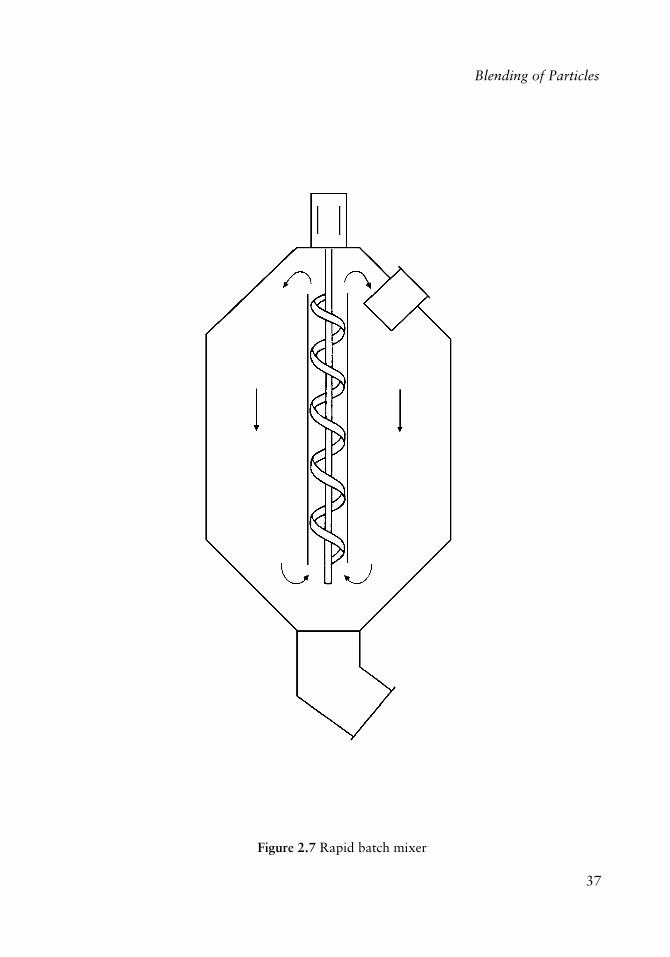
One design of a batch blender is shown schematically in Figure 2.7. Particles are conveyed through a vertical pipe via a screw and then fall freely through the annular region in a recirculating motion. With the equipment marketed by Pari UK [27], the mixer has a capacity of 75 kg.

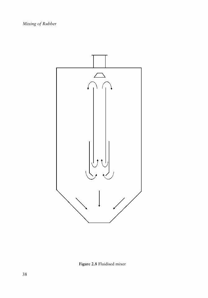
Bayer has developed a large fl uidised bed mixer which can operate continuously and has a capacity of 1000 cubic meters for large scale operations [28]. As seen in Figure 2.8, the basic geometry and particle motion are similar to the Pari mixer.

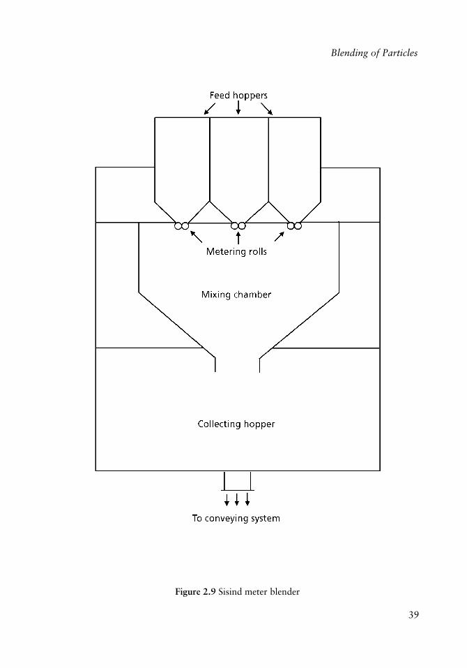
Several manufacturers offer a combination meterer-blender, as shown in Figure 2.9. In these mixers, controlled amounts of the components are metered into a chute by the controlled rotation of neoprene-covered rolls. The particles mix by random tumbling

Table 2.5 Gardner pre-mixerMachine Size Capacity (lb)BB 30

CC 60

DD 100

EE 150

FF 200

GG 300

HH 560

H 560

I 1120

J 1680

K 2240

L 3360

M 4480

37


Figure 2.7 Rapid batch mixer

38

Mixing of Rubber

Figure 2.8 Fluidised mixer

39


Figure 2.9 Sisind meter blender

40

Mixing of Rubber

through the chute into a collection hopper. The mix can then fl ow by gravity into the downstream process or it can be screw-conveyed. The mixer can be operated continuously to give feed rates up to 5000 pounds per hour to supply one or more processing machines.

2.5.4 Equipment Selection

It is diffi cult to provide general guidelines for the selection of particle blenders. If the mixing in downstream process equipment is good so that the blender is only required to provide a roughly constant time-average bulk concentration, the tumble blender is a rugged, simple machine. Of the various shapes available, the rotating cube is often the best shape. Particle segregation by size or density may be a problem.

Ribbon blenders offer superior mixing and the possibility of continuous operation compared with a tumble blender with the penalty of higher capital costs.

Pneumatic mixers can handle large quantities of material continuously but they require careful engineering design. The large mixers are generally suitable only for raw material suppliers who must handle tremendous quantities of granules from their polymer reactor lines.

Meter-blending hoppers offer continuous mixing of a similar quality to tumble blenders with a slightly greater capital cost, which may be offset by lower labour costs and easier handling.

2.6 Summary

In this chapter the statistical theory of mixing has been described. The variance of the distribution of concentrations in a random selection of samples is a useful measure of mixing process. A degree of mixing can be defi ned as the ratio of the variance of the samples to the variance of a perfectly random mixture having the same average concentration. A plot of the degree of mixing defi ned in this way against the mixing time gives a useful description of the kinetics of mixing. Generally, simple mixing can be described by a fi rst-order rate law:

d � / s( )dt

= �k�s

�

��

�

��

eq

�s

�

��

�

��

�

��

�

��

(2.26)

This description of the mixing process does not require any knowledge of the particle kinematics or dynamics of the mixer.

41


Simple statistical descriptions are possible with bicomponent mixtures. With multicomponent mixtures, the process can be described as a Markov chain. The transition probability matrix can be determined experimentally for a mixing operation and this can be used to describe the kinetics of mixing. The same statistical measures are used to describe other mixing operations treated in later chapters where the mechanics may be too complex for analytical model calculations.

A number of different particle blenders have been described; these include tumble blenders, ribbon blenders and pneumatic blenders. The particular choice of blending equipment depends strongly upon the characteristics of the downstream equipment so that no general guidelines are possible.

References

1. P.V. Danckwerts, Applied Polymer Research, 1952, A3, 279.

2. P.M.C. Lacey, Transactions of the Institute of Chemical Engineering, London, 1943, 21, 52.

3. J.P. Beaudry, Chemical Engineering, 1948, 55, 7, 112.

4. C.A. Bennett and N.L. Franklin, Statistical Analysis in Chemistry and the Chemical Industry, John Wiley & Sons Inc., New York, NY, USA, 1963.

5. J.F.E. Adams and A.G. Baker, Transactions of the Institute of Chemical Engineering, 1956, 34, 1, 91.

6. W.D. Mohr, Processing of Thermoplastic Materials, Ed. E.C. Bernhadt, Van Nostrand Reinhold, New York, NY, USA 1959, Chapter 3.

7. S.S. Weidenbaum, Advances in Chemical Engineering, 1958, 2, 211.

8. Chemical Engineers’ Handbooks, 5th Edition, Eds., R.H. Perry and C.H. Chilton, McGraw-Hill Company, New York, NY, USA, 1973.

9. Y. Oyami, Science Papers, Institute of Physical Chemical Research, Tokyo, Japan, 1940, 37, 951, 17.

10. A. Brothman, G.N. Wollan and S.M. Feldman, Chemical and Metallurgical Engineering, 1945, 54, 4, 102.

11. N.K. Maitra and J.M. Coulson, Journal of Imperial College - Chemistry, 1948.

12. P.M.C. Lacey, Journal of Applied Chemistry, 1954, 4, 257.

42

Mixing of Rubber

13. A.S. Michaels and V. Puzinauskas, Chemical Engineering Process, 1954, 50, 12, 604.

14. S.S. Weidenbaum and C.F. Bonilla, Chemical Engineering Process, 1955, 51, 1, 27J.

15. J.C. Smith, Industrial and Engineering Chemistry, 1955, 47, 2240.

16. D. Bustik, ASTM Bulletin, 1950, 165, 66.

17. F.S. Lai and L.T. Fan, Industrial and Engineering Chemistry - Process Design and Development, 1975, 14, 4, 403.

18. M.S. Bartlett, An Introduction to Stochastic Processes, 2nd Edition, Cambridge University Press, UK, 1966.

19. Y. Inoue and K. Yamaguchi, Kagaku Kogaku, 1969, 33, 286.

20. J.M. Coulson and N.K. Maitra, Industrial Chemist, 1950, 11, 2, 55.

21. C.O. Brown, Industrial and Engineering Chemistry, 1950, 42, 7, 57A.

22. Technical Bulletin, Moritz Chemical Engineering Co. Ltd.

23. Technical Bulletin, Baker Perkins Chemical Machinery Ltd.

24. Technical Bulletin, Winkworth Machinery Ltd.

25. Technical Bulletin, Battaggion SpA (Italy).

26. Technical Bulletin, William Gardner & Sons Ltd.

27. Technical Bulletin, Pari UK.

28. J. Schwedes and W. Richter, Chemie Ingenieur Technik, 1975, 47, 295.

43

Laminar and Dispersive Mixing

The various processes required to make a multicomponent polymer-additive system homogeneous can be roughly divided into three types. Simple mixing, discussed in the previous chapter, yields spatial uniformity of the mixture, at least when the samples are viewed on a scale large compared to the size of an individual particle. This kind of mixing may require shear deformation of the polymer, but it does not necessarily occur, as seen for particle blending. Laminar shear mixing does require fl uid fl ow. As will be shown in Section 3.1, this kind of mixing changes the size of the basic fl uid element, the scale of mixing, by altering its shape in shear deformation [1]. The third type of mixing, dispersive mixing, changes the size of particles or agglomerates of particles by fracture or rupture due to the stresses generated during laminar mixing (Section 3.2). This chapter and Chapter 2 describe the basic mixing processes which are used in commercial mixers, as discussed in Chapters 2, 4-6. If any fl uid motion occurs, such as on mills or in internal mixers, all three fundamental processes occur simultaneously. The mixer geometry and operating conditions determine how effi cient a given unit may be in performing these three types of mixing. With particular materials and mixers, one of the three processes may be the rate-determining step in producing a satisfactory product, so that it is convenient to treat the processes separately but it should be remembered that these are parallel processes.

3.1 Laminar Shear Mixing

Chapter 2 considered the random rearrangement of particles throughout the system with no change in size of any individual particle; the scale of mixing rapidly approaches the dimension of a single pellet. To reduce the scale below this level, it is necessary to alter the size of the particles. If the mixture consists of rigid aggregates dispersed through a continuous rubber matrix, then shear stresses exerted on the particles may exceed its cohesive strength and the aggregate will break, as considered in the next section. If the disperse phase is deformable, as shown in Figure 3.1, the initial particle may change its shape without breakup when subjected to a shear fi eld. As the particles deform, their average thickness will decrease as the surface area increases at constant volume and the distance between particles will decrease. Consider two cubes which are initially placed


AuthorAuthor3

44

Mixing of Rubber

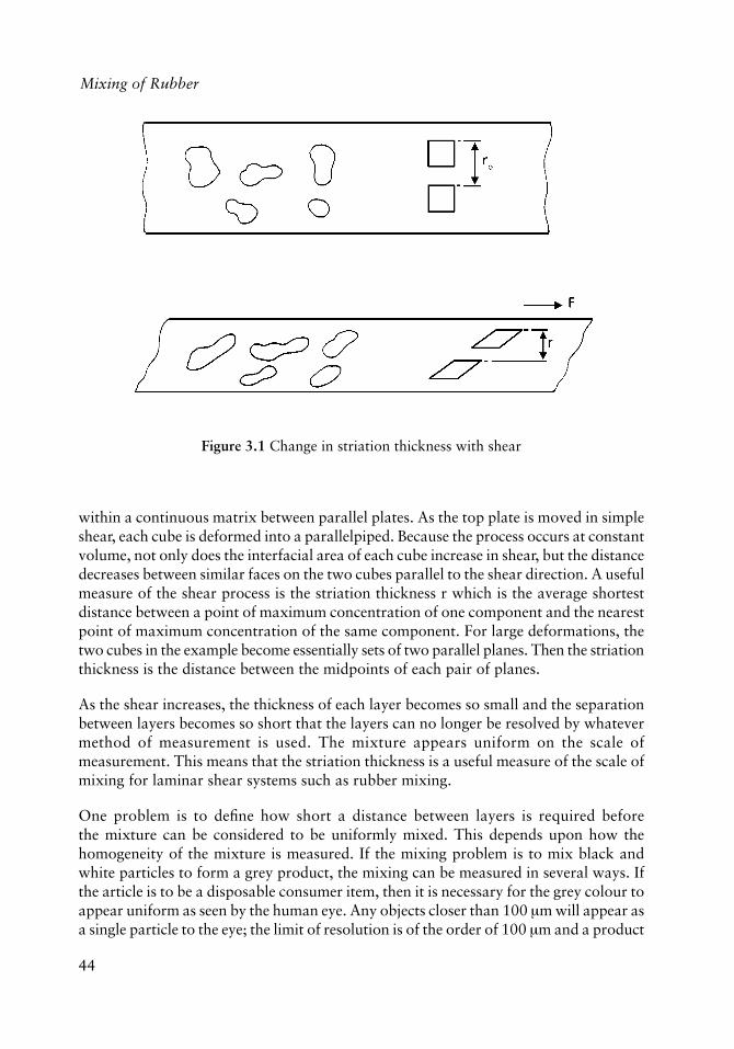
within a continuous matrix between parallel plates. As the top plate is moved in simple shear, each cube is deformed into a parallelpiped. Because the process occurs at constant volume, not only does the interfacial area of each cube increase in shear, but the distance decreases between similar faces on the two cubes parallel to the shear direction. A useful measure of the shear process is the striation thickness r which is the average shortest distance between a point of maximum concentration of one component and the nearest point of maximum concentration of the same component. For large deformations, the two cubes in the example become essentially sets of two parallel planes. Then the striation thickness is the distance between the midpoints of each pair of planes.

As the shear increases, the thickness of each layer becomes so small and the separation between layers becomes so short that the layers can no longer be resolved by whatever method of measurement is used. The mixture appears uniform on the scale of measurement. This means that the striation thickness is a useful measure of the scale of mixing for laminar shear systems such as rubber mixing.

One problem is to defi ne how short a distance between layers is required before the mixture can be considered to be uniformly mixed. This depends upon how the homogeneity of the mixture is measured. If the mixing problem is to mix black and white particles to form a grey product, the mixing can be measured in several ways. If the article is to be a disposable consumer item, then it is necessary for the grey colour to appear uniform as seen by the human eye. Any objects closer than 100 �m will appear as a single particle to the eye; the limit of resolution is of the order of 100 �m and a product

Figure 3.1 Change in striation thickness with shear

45


with a smaller scale of mixing will appear uniform to the unaided eye. If the same object is placed under an optical microscope where the resolution is of the order 1 - 10 �m, the object will now appear non-homogeneous with clumps of black particles randomly placed through a white matrix. Further mixing may reduce the particle size so that they can no longer be resolved in an optical microscope and the product appears uniformly mixed again. However, in an electron microscope where the resolution is of the order 10 - 1000 Å, the product will appear lumpy again. The appearance of homogeneity in a mixture depends upon the relative size of the scale of mixing compared to the resolution of the method of measurement. As long as the scale is smaller than the resolution, the mixture will appear uniform. This enables one to place a quantitative criterion for the degree of mixing as the requirement that the scale of mixing be less than the resolution of the method of measurement.

3.1.1 Calculation of Striation Thickness

As the area of each cube in the example of Figure 3.1 increases, the striation thickness decreases [2-5] For a constant volume process:

v – r A /2 (3.1)

where the total volume V is for a region enclosed by interfacial area A and having striation thickness r. The factor of two appears because each layer has two interfaces. The problem of laminar shear mixing is how to calculate the change in interfacial area, hence the striation thickness, for the shear fi eld in a given mixer geometry.

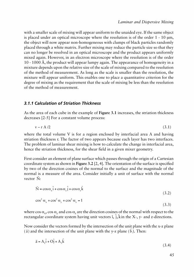
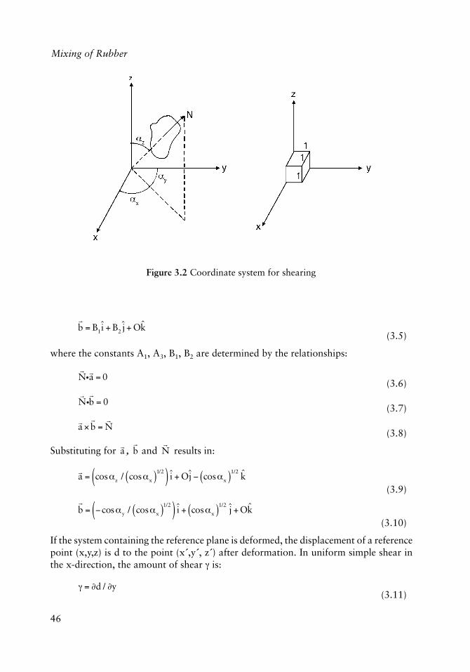
First consider an element of plane surface which passes through the origin of a Cartesian coordinate system as shown in Figure 3.2 [2, 4]. The orientation of the surface is specifi ed by two of the direction cosines of the normal to the surface and the magnitude of the normal is a measure of the area. Consider initially a unit of surface with the normal vector

�

N:

�

N = cos�x i + cos�y j + cos�zk (3.2)

cos2 �x + cos2 �y + cos2 �z = 1

(3.3)

where cos �x, cos �y and cos �z are the direction cosines of the normal with respect to the rectangular coordinate system having unit vectors î, j , k in the X-, y- and z-directions.

Now consider the vectors formed by the intersection of the unit plane with the x-z plane ( �a) and the intersection of the unit plane with the y-z plane (

�

b ). Then:

�a = A1i + Oj + A3k

(3.4)

46

Mixing of Rubber

�

b = B1i + B2 j + Ok (3.5)

where the constants A1, A3, B1, B2 are determined by the relationships:

�

Ni�a = 0

(3.6)

�

Ni

�

b = 0 (3.7)

�a��

b =�

N (3.8)

Substituting for �a , �

b and �

N results in:

�a = cos�z / cos�x( )1/2( ) i + Oj cos�x( )1/2

k (3.9)

�

b = cos�y / cos�x( )1/2( ) i + cos�x( )1/2j + Ok

(3.10)

If the system containing the reference plane is deformed, the displacement of a reference point (x,y,z) is d to the point (x�,y�, z�) after deformation. In uniform simple shear in the x-direction, the amount of shear � is:

� = �d / �y

(3.11)

Figure 3.2 Coordinate system for shearing

47


If the origin is not displaced then

dx = �yi (3.12)

Vector �a remains unchanged by the deformation because it lies in the x-z plane which

is undistorted by shear. The vector �

b transforms as:

�

�b =�

b + dx

=�

b + �yi

= � cos�x( )1/2 cos�y / cos�x( )1/2( ) i + cos�x( )1/2

j (3.13)

Then the area of the plane is given as:

�A =��a ��

�b (3.14)

Since the plane initially had unit area, the ratio becomes:

�AA

=

��a ��

�b

1

= 1 2� cos�x cos�y + �2 cos2 �x( )1/2

(3.15)

Because of the inverse relationship between area and striation thickness:

�r =ro

1 2� cos�x cos�y + �2 cos2 �x( )1/2

(3.16 )

which decreases with the increase in total shear �. In addition, Equation (3.15) shows that the change in area depends strongly on the orientation of the surface relative to the shear direction.

Now consider a mixture of discrete cubes of uniform size whose centres are randomly distributed throughout the material, each with its edges parallel to the coordinate axes. The direction cosines of each face are:

x y plane : cos�x = cos�y = 0 cos�z = 1

y z plane : cos�x = 1 cos�y = cos�z = 0

x z plane : cos�x = 0 cos�y = 1 cos�z = 0

�

��

�� (3.17)

Each face has an initial area ao which, on deformation in simple shear, becomes:

48

Mixing of Rubber

x y plane : axy / ao( )2= 1

y z plane : ayz / ao( )2= 1+ �2

x z plane : axz / ao( )2= 1

�

�

��

�

�� (3.18)

The total area before and after deformation are:

Ao = 6Nao

A = 2N axy + ayz + axz( )��

�� (3.19)

where N is the number of cubes. Then the ratio of areas becomes:

AAo

=13

+13

1+ �2( )1/2

+13

(3.20 )

For most practical mixing problems, the total shear is large so:

AAo

��3

(3.21)

The initial surface-to-volume ratio of the mixture is:

Ao

V= 6ao / ao

32 / Y( )= 6Y / �

(3.22)

where Y is the volume fraction of cubes having an edge length � = ao

1/2. Substituting Equations (3.1) and (3.22) into Equation (3.21) yields an expression for striation thickness:

r = 2V/A

= 2 V/Ao( ) / A/Ao( )= � / �Y

(3.23)

This analysis has assumed that the viscosity of the continuous and dispersed phases are identical, which is a reasonable approximation for mixing a masterbatch in a rubber matrix. However, if the dispersed phase is a low viscosity liquid or a high viscosity solid, mixing may be more diffi cult.

Consider the case shown in Figure 3.3. Two layers of one material A, each having a thickness �1, are separated by a layer of a second material B having a thickness �2. The two materials are identical in every respect except for their viscosities �A and �B. The

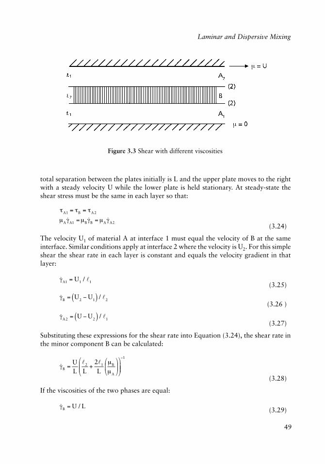
49


total separation between the plates initially is L and the upper plate moves to the right with a steady velocity U while the lower plate is held stationary. At steady-state the shear stress must be the same in each layer so that:

�A1 = �B = �A2

�A ��A1 =�B ��B = �A ��A2 (3.24)

The velocity U1 of material A at interface 1 must equal the velocity of B at the same interface. Similar conditions apply at interface 2 where the velocity is U2. For this simple shear the shear rate in each layer is constant and equals the velocity gradient in that layer:

��A1 = U1 / �1 (3.25)

��B = U2 U1( ) / �2

(3.26 )

��A2 = U U2( ) / �1

(3.27)

Substituting these expressions for the shear rate into Equation (3.24), the shear rate in the minor component B can be calculated:

��B =UL

�2

L+

2�1

L�B

�A

�

��

�

�

�

��

�

�

1

(3.28)

If the viscosities of the two phases are equal:

��B = U / L (3.29)

Figure 3.3 Shear with different viscosities

50

Mixing of Rubber

which is the uniform shear fi eld used in the previous calculation. If the viscosity of the minor component becomes very large, as with a solid:

�B / �A ��

��B �0 (3.30)

so little shear mixing occurs in the minor component. On the other hand, for low viscosity liquids in rubber:

�B / �A = 0

��B �U / �2 (3.31)

so that the shear mixing depends only upon the initial particle size �2 and the velocity of the boundaries of the apparatus U. Because of this behaviour with a mismatch in viscosities, liquids can often be easily mixed into a rubber matrix but rigid aggregates require a masterbatch intermediate for good mixing. Large deformations of the rubber matrix, which consume much energy, are required to achieve small shear deformations in the rigid minor phase.

3.1.2 The Effect of Streamline Orientation

The relative orientation of the surface of the disperse phase element to the fl ow streamline is important in ensuring good laminar mixing [6]. In the simple Couette fl ow shown in Figure 3.4, the outer cylinder rotates about the inner cylinder with a constant angular velocity �. Because of the fl ow symmetry, all streamlines are circles concentric with the cylinders. If a thin concentric circle of tracer is placed in the fl uid, the normal to the tracer surface is orthogonal to the streamlines:

cos�r = cos�z = 0

cos�� = 1

�A / A = 1 (3.32)

and no shear mixing occurs. If the tracer is placed in a plane containing the cylinder axis:

cos�� = cos�z = 0

cos�r = 1

�A / A�= � = R�t (3.33)

If the tracer only partially crosses the annulus, then only a ring of mixed material forms because there is no radial velocity component. This simple experiment illustrates the

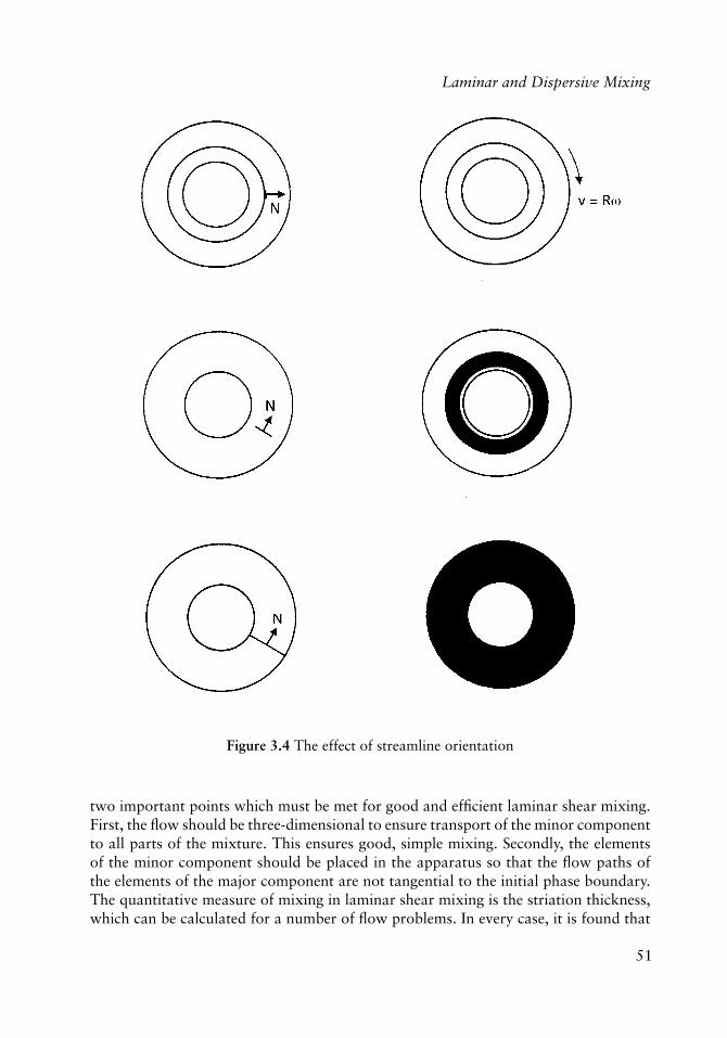
51


two important points which must be met for good and effi cient laminar shear mixing. First, the fl ow should be three-dimensional to ensure transport of the minor component to all parts of the mixture. This ensures good, simple mixing. Secondly, the elements of the minor component should be placed in the apparatus so that the fl ow paths of the elements of the major component are not tangential to the initial phase boundary. The quantitative measure of mixing in laminar shear mixing is the striation thickness, which can be calculated for a number of fl ow problems. In every case, it is found that

Figure 3.4 The effect of streamline orientation

52

Mixing of Rubber

the striation thickness is a function of the total shear strain and not just the shear rate. To maintain the same degree of mixing in scale-up, it is necessary to maintain the fi nal striation thickness, which means maintaining a constant total shear (See Chapter 5). In uniform shear fi elds there is no ambiguity to this statement, but in the non-uniform fl ow fi elds characteristic of mixing equipment, it is necessary to select a characteristic shear strain to use in scale-up. The maximum deformation occurs at a moving boundary, but because of complex fl ows, this may not be characteristic of the bulk fl ow. Therefore, it is more appropriate to use a value averaged over the bulk of the material:

� =

�v�dVV

(3.34)

where V is the volume of the mixture. It will be seen that this criterion differs from the scale-up rule used when particle or agglomerate rupture is controlling the goodness of mixing. Then it is necessary to maintain the maximum shear stress constant in scale-up.

3.2 Dispersive Mixing

Solid particle additives are incorporated into the rubber matrix to increase the mechanical strength, to colour the product, to reduce cost or to protect from environmental attack. These additives may be mixed directly into the product in the processing line. A masterbatch, which is an intermediate mixture with a high additive concentration, is often prepared fi rst and then diluted in the rubber matrix in the fi nal processing. The advantages of masterbatches are discussed in a later section.

The operation of mixing solid additives can be considered as two simultaneous processes. First, the solids initially incorporated into the rubber matrix may have too large a size because of incomplete milling by the supplier or compaction during shipment. More commonly, the particles initially form aggregates and agglomerates when incorporated into the rubber matrix and these secondary units must be reduced in size. This problem will be illustrated in Section 3.4 for the mixing of carbon black in rubber. In the case of pigments, the largest particles must be smaller than the limit of resolution by the eye if the product is to appear uniform. Particles must be small enough so that those near the surface do not protrude to give roughness or a matte fi nish where surface gloss is important. Carbon black and other reinforcing agents increase in effectiveness with higher surface-to-volume ratios of small particles. The particle size requirements may not have a simple physical interpretation as with pigments, but in every case a quantitative criterion can be established experimentally for the design or control of a mixing process. The break-up of particles and agglomerates in rubber requires large expenditures of energy because of the high viscosity of the matrix, so that equipment design and operating conditions must be set to meet the criteria without reducing particle sizes unnecessarily.

53


The second process is to disperse the particles evenly throughout the bulk of the rubber to eliminate gross heterogeneities. In the case of small, non-interacting particles, the additive will follow the streamlines of the fl owing rubber and the problem is one of laminar mixing described above. If the particles interact, either through direct cohesive forces or through tie molecules of rubber, their trajectories are more complicated than for streamline fl ow. In principle, these trajectories can be calculated but the complex geometry of mixing equipment makes the calculations intractable in practice. By analysis of the idealised break-up and separation of particles, the physical principles of dispersive· mixing can be elucidated. As will be shown in subsequent sections, these can lead to confl icting requirements for equipment design, operation and scale-up which can only be resolved by using masterbatches.

3.2.1 Calculation of Forces on a Particle

The additive aggregate may consist of an agglomeration of particles held together by static charge accumulation on the surface or by tie rubber molecules, or it may be a single large particle which must be fractured into smaller fragments. In this case, it is convenient to consider the single large particle as if it were an agglomerate of smaller particles. Then the difference between aggregates and agglomerates can be considered to be solely a function of the inter-particle force which is large for aggregates and relatively weak for agglomerates. To elucidate the principles of dispersion, consider the aggregate as a pair of spheres of the primary particle with equal radii (R) as shown in Figure 3.5. The particle dimensions are small compared to the narrowest fl ow channel so the particles can be considered to be in an infi nite medium [7]. The pair of particles are suspended in the uniform simple shear fi eld of a Newtonian fl uid. The closest approach of the centres of the particles is 2R. For a separation of centres between 2R and r*, the force of attraction is considered constant and the force is negligible for larger separations. Then using the centre of one particle as the origin of a Cartesian coordinate system, the second particle has its centre located at:

R2 = x2 + y2 (3.34)

and the forces are:

F = Fa 2R < r < r* (3.35)

F = -� r < 2R (3.36)

F = 0 r > r* (3.37)

The fl uid velocity relative to the reference streamline which follows the centre of the fi rst particle:

� = ��y

(3.38)

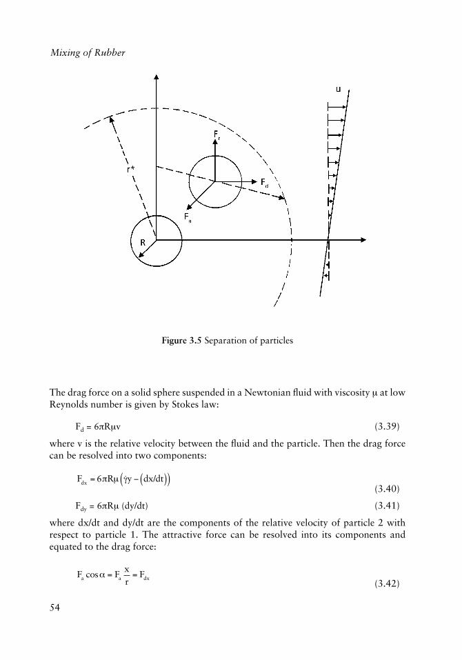
54

Mixing of Rubber

The drag force on a solid sphere suspended in a Newtonian fl uid with viscosity � at low Reynolds number is given by Stokes law:

Fd = 6�R�v (3.39)

where v is the relative velocity between the fl uid and the particle. Then the drag force can be resolved into two components:

Fdx = 6�R� ��y � dx/dt( )( )

(3.40)

Fdy = 6�R� (dy/dt) (3.41)

where dx/dt and dy/dt are the components of the relative velocity of particle 2 with respect to particle 1. The attractive force can be resolved into its components and equated to the drag force:

Fa cos� = Fa

xr

= Fdx

(3.42)

Figure 3.5 Separation of particles

55


Fa sin� = Fa

yr

= Fdy

(3.43)

where � is the angle of the line connecting the particle centres. These last two equations can be combined to eliminate dt to yield:

dxdy

xy

= Kr

(3.44)

where K = K = 6�R�� / Fa

which describes the particle trajectories. If the approximation is made that:

r � x + y

then Equation (3.44) becomes linear:

dxdy

+ x K 1y

�

��

�

�� = Ky

(3.45)

which can be solved analytically as:

x + yy

= CeKy

(3.46)

where C is a constant of integration. If the particle centre must pass through the point (xo, yo)’ then C is specifi ed and:

x + yxo + yo

yo

y= exp Kyo 1

yyo

�

��

�

��

�

��

�

��

(3.47)

Using this equation, the particle trajectories could be calculated which allow some qualitative conclusions.

First, high shear stresses, which mean large K, increase the dispersion. Low interparticle attraction also means high K and better dispersion. For a given particle attraction, there is a critical stress below which dispersion will not occur. For shear stresses only slightly above the critical value, dispersion is sensitive to the relative orientation of the particles to the fl ow fi eld. Larger particles have a higher K and disperse more rapidly. Finally, if the fl ow in the mixer is unidirectional, only particles favourably aligned initially will be dispersed. The remainder will be aligned with the fl ow and will not be separated unless the fl ow changes direction.

56

Mixing of Rubber

This analysis has assumed the uniform simple fl ow of a Newtonian liquid and the simple creeping fl ow past a sphere, neglecting hydrodynamic interaction between spheres. Although the conditions in a rubber mixture are far more complicated, the essential points developed in this treatment would remain unchanged with a rigorous analysis. In an internal mixer, mill or extruder, the average channel depths are large compared to the particle size in order to achieve high throughputs. The shear stresses in these deep channels are low so that a region in the mixer with a narrow gap must be provided to obtain the high stresses necessary for particle or agglomerate rupture and dispersion. In subsequent chapters when specifi c equipment designs are considered, it will often be seen that the performance of a mixer is critically dependent on the design of these narrow gaps even though they may only occupy a small fraction of the mixer volume.

3.2.2 Flow in Thin Channels

The idealised treatment of the effect of the narrow gap at the tip of the blade in an internal mixer was derived by Bolen and Colwell [8], as discussed in detail in Chapter 5. The importance of this fl ow region can be seen by considering the fl ow past a blade tip shown schematically in Figure 3.6. Using the lubrication approximation to simplify the analysis [9, 10, 11], it can be shown as in Chapter 4 and 5 that the volumetric fl ow rate Q per unit axial length for a constant channel depth h is given by:

Q =

h2U

h3

12�dpdx

�

��

�

��

(3.48)

for a tip velocity U and pressure gradient dp/dx. If the channel depth varies slowly with position, this equation applies locally at each point. The x-component of velocity u becomes:

u = U 1

yh

�

��

�

��

h2

2�yh

y2

h2

�

��

�

��

dpdx

(3.49)

and the shear stress T becomes:

� = �dudy

= �Uh

+h2

dpdx

12yh

�

��

�

�

(3.50)

Solving Equation (3.48) for the pressure gradient yields:

dpdx

= 6�Uh2

2Qh3

�

��

�

�� (3.51)

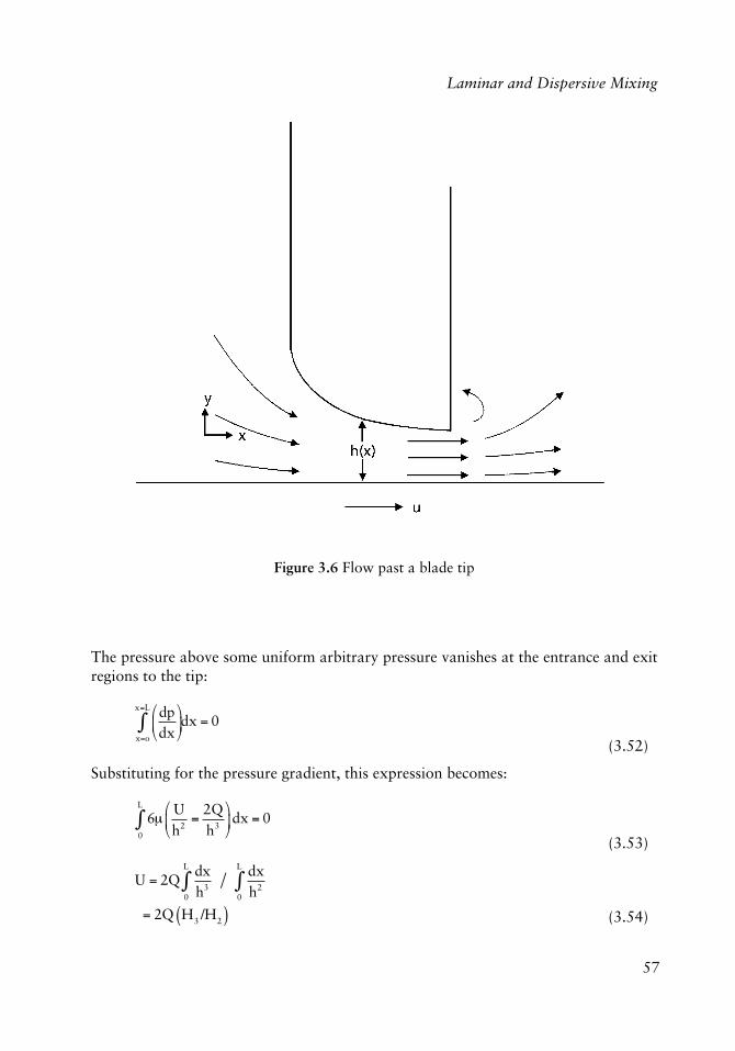
57


The pressure above some uniform arbitrary pressure vanishes at the entrance and exit regions to the tip:

dpdx

�

��

�

��

x=o

x=L

� dx = 0

(3.52)

Substituting for the pressure gradient, this expression becomes:

6�

Uh2

=2Qh3

�

��

�

��dx = 0

0

L

� (3.53)

U = 2Qdxh3

0

L

� dxh2

0

L

�

= 2Q H3 /H2( ) (3.54)

Figure 3.6 Flow past a blade tip

58

Mixing of Rubber

where Hn = dx / hn�

and h may vary with position x. Substituting these expressions into the shear stress equation yields:

� =

6�Qh2

8�QH3

hH2

12�Q

hyh

�

��

��

H3

H2

1h

�

��

�

��

(3.55)

The maximum shear stress occurs at the blade tip where y = h:

�max =

6�Qh2

8�Q

hH3

H2 (3.56)

If the channel depth is constant, then the maximum shear stress varies inversely with the square of the gap so that the high shear stresses for particle dispersion require narrow gaps.

Although the fl ow between the blade tip and the wall or the nip region of a mill is predominantly a shear fl ow, there is an elongational fl ow component due to the contraction of the fl ow channel at the nip entrance. The forces generated by elongational fl ow are signifi cantly higher but the kinematics of the velocity fi eld play a crucial role. Kao and Mason [12] studied the dispersion of a suspension of polymethylmethacrylate (PMMA) beads in a silicone oil. The fl uid was a Newtonian liquid having � = 100 cp. The PMMA beads initially formed a compact aggregate in the fl uid and the aggregate size R was measured as a function of the total strain

��t generated in a shear fl ow:

u = ��y (3.57)

V = 0 (3.58)

and the strain generated in an elongational fl ow:

u = ��x / 2 (3.59)

V = ��x / 2 (3.60)

As shown in Figure 3.7, the elongational fl ow fi eld was signifi cantly more effi cient in particle dispersion than the shear fl ow. In the shear fl ow, the aggregate rotated and wobbled. Occasionally a particle separated from the aggregate and was swept away but there was no general break-up and dispersion of the aggregate. In contrast, with elongational fl ow particles were pulled directly from the aggregate which rapidly dispersed. The aggregate size closely followed the expression:

R0

3 Rt3( ) = k��t

(3.61)

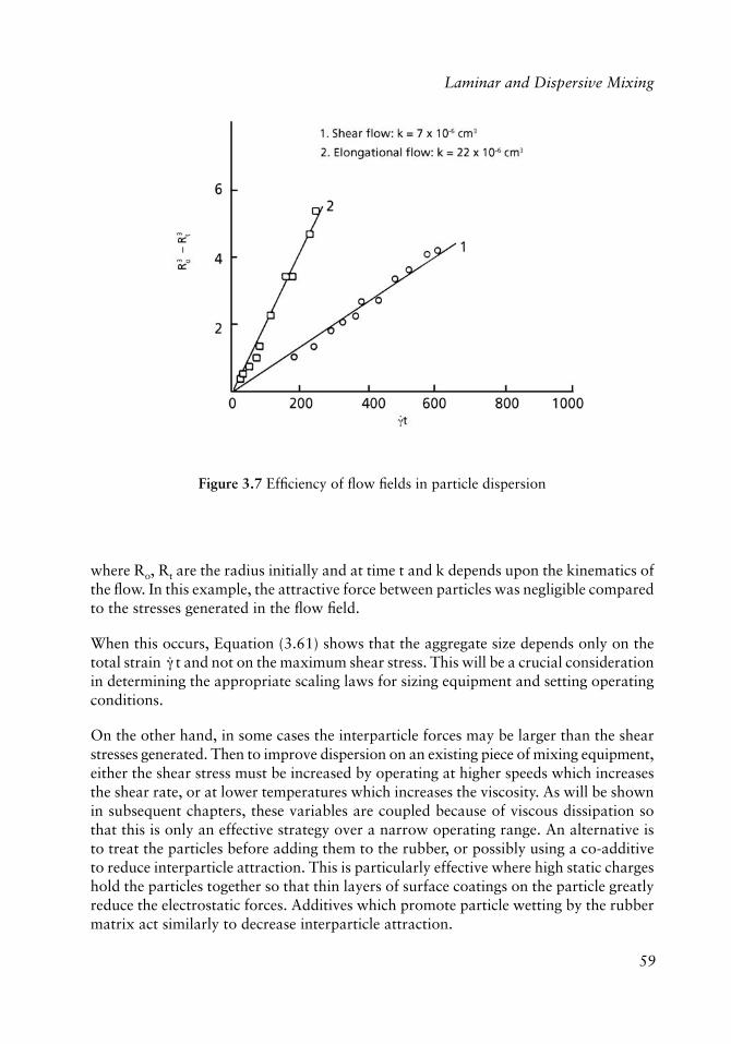
59


where Ro, Rt are the radius initially and at time t and k depends upon the kinematics of the fl ow. In this example, the attractive force between particles was negligible compared to the stresses generated in the fl ow fi eld.

When this occurs, Equation (3.61) shows that the aggregate size depends only on the total strain

�� t and not on the maximum shear stress. This will be a crucial consideration

in determining the appropriate scaling laws for sizing equipment and setting operating conditions.

On the other hand, in some cases the interparticle forces may be larger than the shear stresses generated. Then to improve dispersion on an existing piece of mixing equipment, either the shear stress must be increased by operating at higher speeds which increases the shear rate, or at lower temperatures which increases the viscosity. As will be shown in subsequent chapters, these variables are coupled because of viscous dissipation so that this is only an effective strategy over a narrow operating range. An alternative is to treat the particles before adding them to the rubber, or possibly using a co-additive to reduce interparticle attraction. This is particularly effective where high static charges hold the particles together so that thin layers of surface coatings on the particle greatly reduce the electrostatic forces. Additives which promote particle wetting by the rubber matrix act similarly to decrease interparticle attraction.

Figure 3.7 Effi ciency of fl ow fi elds in particle dispersion

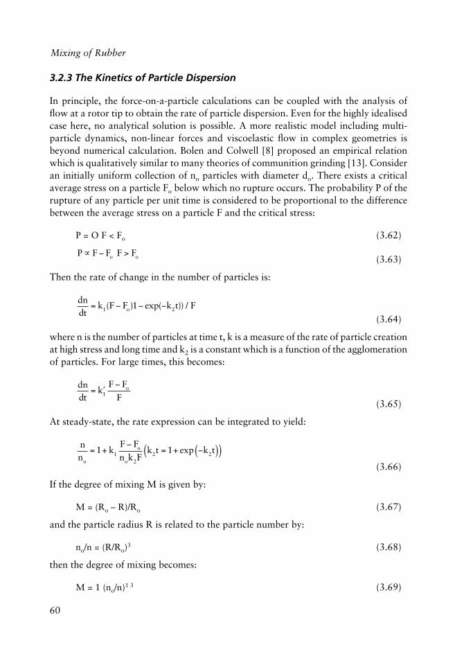
60

Mixing of Rubber

3.2.3 The Kinetics of Particle Dispersion

In principle, the force-on-a-particle calculations can be coupled with the analysis of fl ow at a rotor tip to obtain the rate of particle dispersion. Even for the highly idealised case here, no analytical solution is possible. A more realistic model including multi-particle dynamics, non-linear forces and viscoelastic fl ow in complex geometries is beyond numerical calculation. Bolen and Colwell [8] proposed an empirical relation which is qualitatively similar to many theories of communition grinding [13]. Consider an initially uniform collection of no particles with diameter do. There exists a critical average stress on a particle Fo below which no rupture occurs. The probability P of the rupture of any particle per unit time is considered to be proportional to the difference between the average stress on a particle F and the critical stress:

P = O F < Fo (3.62)

P� F Fo F > Fo (3.63)

Then the rate of change in the number of particles is:

dndt

= k1(F Fo)1 exp(k2t)) / F

(3.64)

where n is the number of particles at time t, k is a measure of the rate of particle creation at high stress and long time and k2 is a constant which is a function of the agglomeration of particles. For large times, this becomes:

dndt

= �k1

F Fo

F (3.65)

At steady-state, the rate expression can be integrated to yield:

nno

= 1+ k1

F Fo

nok2Fk2t = 1+ exp k2t( )( )

(3.66)

If the degree of mixing M is given by:

M = (Ro – R)/Ro (3.67)

and the particle radius R is related to the particle number by:

no/n = (R/Ro)3 (3.68)

then the degree of mixing becomes:

M = 1 (no/n)1 3 (3.69)

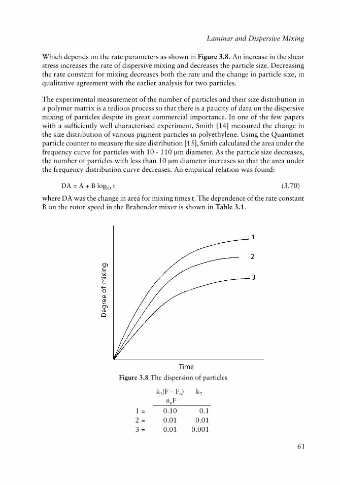
61


Which depends on the rate parameters as shown in Figure 3.8. An increase in the shear stress increases the rate of dispersive mixing and decreases the particle size. Decreasing the rate constant for mixing decreases both the rate and the change in particle size, in qualitative agreement with the earlier analysis for two particles.

The experimental measurement of the number of particles and their size distribution in a polymer matrix is a tedious process so that there is a paucity of data on the dispersive mixing of particles despite its great commercial importance. In one of the few papers with a suffi ciently well characterised experiment, Smith [14] measured the change in the size distribution of various pigment particles in polyethylene. Using the Quantimet particle counter to measure the size distribution [15], Smith calculated the area under the frequency curve for particles with 10 - 110 �m diameter. As the particle size decreases, the number of particles with less than 10 �m diameter increases so that the area under the frequency distribution curve decreases. An empirical relation was found:

DA = A + B loglO t (3.70)

where DA was the change in area for mixing times t. The dependence of the rate constant B on the rotor speed in the Brabender mixer is shown in Table 3.1.

Figure 3.8 The dispersion of particles

k1(F – Fo) k2

noF

1 = 0.10 0.12 = 0.01 0.013 = 0.01 0.001

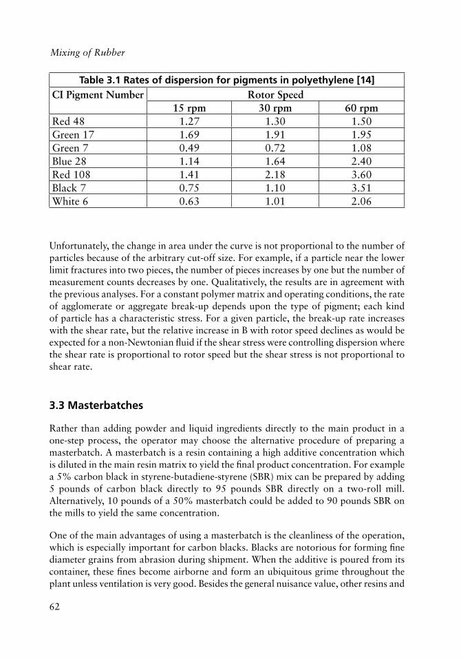
62

Mixing of Rubber

Table 3.1 Rates of dispersion for pigments in polyethylene [14]CI Pigment Number Rotor Speed

15 rpm 30 rpm 60 rpmRed 48 1.27 1.30 1.50Green 17 1.69 1.91 1.95Green 7 0.49 0.72 1.08Blue 28 1.14 1.64 2.40Red 108 1.41 2.18 3.60Black 7 0.75 1.10 3.51White 6 0.63 1.01 2.06

Unfortunately, the change in area under the curve is not proportional to the number of particles because of the arbitrary cut-off size. For example, if a particle near the lower limit fractures into two pieces, the number of pieces increases by one but the number of measurement counts decreases by one. Qualitatively, the results are in agreement with the previous analyses. For a constant polymer matrix and operating conditions, the rate of agglomerate or aggregate break-up depends upon the type of pigment; each kind of particle has a characteristic stress. For a given particle, the break-up rate increases with the shear rate, but the relative increase in B with rotor speed declines as would be expected for a non-Newtonian fl uid if the shear stress were controlling dispersion where the shear rate is proportional to rotor speed but the shear stress is not proportional to shear rate.

3.3 Masterbatches

Rather than adding powder and liquid ingredients directly to the main product in a one-step process, the operator may choose the alternative procedure of preparing a masterbatch. A masterbatch is a resin containing a high additive concentration which is diluted in the main resin matrix to yield the fi nal product concentration. For example a 5% carbon black in styrene-butadiene-styrene (SBR) mix can be prepared by adding 5 pounds of carbon black directly to 95 pounds SBR directly on a two-roll mill. Alternatively, 10 pounds of a 50% masterbatch could be added to 90 pounds SBR on the mills to yield the same concentration.

One of the main advantages of using a masterbatch is the cleanliness of the operation, which is especially important for carbon blacks. Blacks are notorious for forming fi ne diameter grains from abrasion during shipment. When the additive is poured from its container, these fi nes become airborne and form an ubiquitous grime throughout the plant unless ventilation is very good. Besides the general nuisance value, other resins and

63


products pick up these particles which can cause serious contamination. Many companies avoid this problem by using a special area for the preparation of black compounding which effectively isolates the dirt in one small section of the plant. Once the black has been incorporated into a resin, even at high concentration, it may safely be transferred to other sections of the plant without further dirt problems. Thus masterbatches permit the use of carbon black compounds with a minimum cost to prevent contamination.

Most other additives do not present the same potential for contamination as carbon black. Preparing a masterbatch inserts an extra processing step into the manufacturing line which represents a premium on the manufacturing costs. Therefore the decision to use a masterbatch must have a strong technological justifi cation.

One of the major problems with additives in continuous mixing such as in an extruder is to maintain a steady feed rate of the additive. It is easy to fi ll the feed hopper with a bag of resin or to feed continuously with a strip from an upstream process. Additives used in small amounts must be added intermittently in moderate amounts or small amounts added continuously. In the fi rst case, there must be signifi cant backmixing in the extruder for uniform dispersion but most extruders and other continuous mixers are designed to minimise gross backmixing. Continuous feeding at small rates is often unsatisfactory because the additive is in a physical state which is diffi cult to pump and meter. To overcome these problems, a highly concentrated masterbatch can be prepared in the form of pellets which are then blended with the base resin in a solid blending operation, as described in Chapter 2. The blend is then fed to the continuous process. With internal mixers, such as the Banbury mixer, the operation is essentially a batch process so that the problem of metering and intermediate additive feed does not arise.

Even with batch internal mixers, the requirement of high stress for the rupture of additive particles may dictate the use of masterbatches. To impose a high stress on the particle means that the rubber matrix must be subjected to a high shear rate. The concomitant viscous dissipation in the shear fi eld will raise the temperature of the batch. In large mixers especially, the heat transfer will be relatively poor so that the temperature rise accompanying the mixing for particle dispersion may cause degradation, or scorchiness if vulcanising agents are present. The high shear stresses necessary for particle rupture also require relatively small clearances between the rotor fl ight tip and the chamber wall. As discussed in Chapter 5, the elastic component of the viscoelastic behaviour of rubber will be more important in larger mixers so that the dispersion will be less effi cient in a smaller mixer. Finally, a signifi cant fraction of the energy input to the matrix is dissipated as heat rather than being transmitted to the particle for fracture.

The effi ciency of energy transfer to the dispersed phase can be approximately calculated using the system of Figure 3.3 and Equations (3.24)-(3.29). The energy dissipated per unit volume in each phase E can be calculated as:

64

Mixing of Rubber

EA = 2�A ��A1

= 2�A��A12

(3.71)

and

EB = �B ��B

= �B ��B2

(3.72)

where the factor 2 occurs because of the two layers of material A. Then the fraction of energy transferred to the disperse phase B is:

f =EBVB

EAVA

=�B ��B

2�2S

2�A ��A1�1S

=�B�2

2�A�1

��B2

��A2

(3.73)

where S is the interface area between layers. Substituting into this expression yields:

f =

�A�2

2�B�1 (3.74)

For the dispersion of particles into rubber:

�A <�B

�2 << �1

f <<1 (3.75)

Therefore only a small fraction of the shear energy is transmitted to the particle.

The less rubber in the mix during particle fracture, the more effi cient will be the use of energy. This may be a signifi cant cost savings in favour of the use of masterbatches. Ideally the feed particles will have the correct size distribution, accounting for the inevitable changes occurring in the mixing apparatus, so that the mixer need only be designed and operated for laminar shear mixing. This can be more readily accomplished with masterbatches.

65


3.4 Incorporation of Carbon Black

One of the single most important operations in the rubber industry is the mixing of carbon black into a rubber matrix. Most articles in the literature concentrate on the effect of compounding changes on rubber properties. However, for any product formulation, the fl uid mechanical processes occurring in the mixing stage, the subject of this monograph, determines the uniformity of distribution of ingredients for homogeneous crosslinking as well as the shape and size of fi ller domains for reinforcement. Mixing has a direct effect on the product properties by controlling the fi ller dispersion.

Fedyukin and co-workers [16] dispersed zinc oxide and vulcanising agents in either oil or water latex of polyisoprene (PIP), or the additives were used as a powder. These were mixed with PIP on a mill. The latex-dispersed additives had the smallest initial particle size and the powder had the largest particles. The number of fi ller particles was largest for the latex while the particle size and distance between particles was smallest for this system. The reverse was true for the powder. The smaller latex-prepared particles gave the most rapid network formation, the most uniform distribution of crosslinks and the most elastic network. All of these properties correlated with the particle size of the dispersed phase.

Many mechanical properties of a fi lled rubber are functions of the volume fraction of fi ller particles. For example, the Guth-Gold equation predicts the stiffening effect of fi llers on the modulus [17, 18]:

Ef = Eg(1 + 2.5� + 14.1�2) (3.76)

where Ef is the modulus of the fi lled rubber having an unfi lled modulus Eg and having a volume fraction � of fi ller. When the volume fraction of fi ller alone is used, the equation is inadequate but Medalia introduced the concept of occluded rubber which states that the fi ller acts as if it had an effective volume �e:

�e = � + �o (3.77)

where �o is the occluded rubber volume fraction. The occluded rubber model asserts that a fraction of the rubber is effectively immobilised in the interstices of the secondary carbon black particle which has a convoluted, open shape. The immobilised molecules tie several particles together which form agglomerates whose size is larger than the sum of the volumes of the particles alone. These agglomerates act as a structural unit in the matrix, and hence they are the relevant particles to consider in theories of reinforcement. The effective volume depends upon the ‘structure’ of the carbon black, which is a rough description of the architecture of secondary particles. The effective volume fraction can be calculated from the results of the standard dibutyl phosphate (DBP) absorption test:

�e = �(1 + 0.2139 DBP)/1.46 (3.78)

where DBP is the amount of DBP absorbed in a standard laboratory test [19].

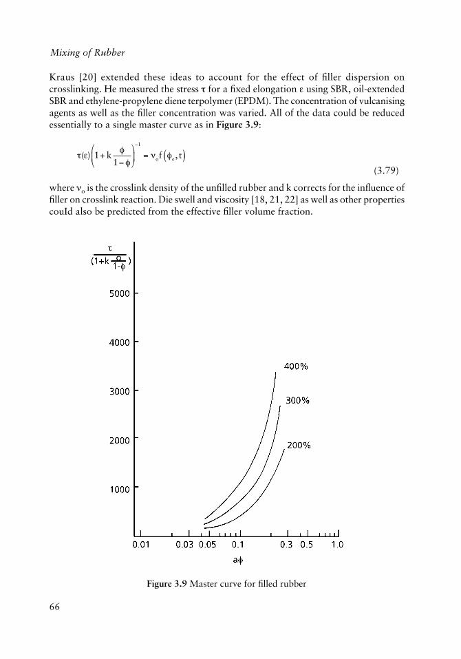
66

Mixing of Rubber

Kraus [20] extended these ideas to account for the effect of fi ller dispersion on crosslinking. He measured the stress � for a fi xed elongation � using SBR, oil-extended SBR and ethylene-propylene diene terpolymer (EPDM). The concentration of vulcanising agents as well as the fi ller concentration was varied. All of the data could be reduced essentially to a single master curve as in Figure 3.9:

�(�) 1+ k

�1 �

�

��

�

1

= �of �e, t( ) (3.79)

where !o is the crosslink density of the unfi lled rubber and k corrects for the infl uence of fi ller on crosslink reaction. Die swell and viscosity [18, 21, 22] as well as other properties couId also be predicted from the effective fi ller volume fraction.

Figure 3.9 Master curve for fi lled rubber

67


At the beginning of the compounding step, the carbon black is completely segregated from the rubber matrix. At fi rst the rubber is folded over large clumps of carbon black which then break into more fi nely divided agglomerates dispersed through the bulk of the rubber, the ‘occluded rubber’ particles. These are large compared to the size of individual aggregate particles and to the steady-state size of aggregate domains. This inclusion step corresponds to the fi rst power peak observed in an internal mixer (Figure 5.2). With continued shearing the aggregates are pulled apart, the number of particles increases, the particle size decreases and the effective volume fraction increases. Therefore all properties which depend upon the effective volume fraction, such as die swell and Mooney viscosity, will depend on the amount of mixing (Figure 4.4).

3.5 Summary

The principal task of the mixing operation is to incorporate additives into the base material. This may involve masterbatches, which can be particularly effi cient for particle dispersion, or one-step processes. The additive must be uniformly distributed throughout the bulk of the rubber and the particle size must be suffi ciently small to give homogeneous properties. If the shear stresses are suffi ciently high so that particles rupture readily, then the total shear strain in laminar shear mixing determines the degree of mixing. If relatively strong particles must be reduced in size, then the maximum shear stress generated in the apparatus becomes important. In either case, the product properties critically depend upon the mixing process.

References

1. P.V. Danckwerts, Chemical Engineering Science, 1953, 2, 1.

2. R.S. Spencer and R.M. Wiley, Journal of Colloid Science, 1951, 6, 133.

3. W.D. Mohr, R.L. Saxton and C.H. Jepson, Industrial and Engineering Chemistry, 1957, 49, 1855.

4. W.D. Mohr in Processing of Thermoplastic Materials, Ed., E.C. Bernhardt, Van Nostrand Reinhold, New York, NY, USA, 1959, Chapter 3.

5. H.F. Irving and R.L. Saxton in Mixing: Theory and Practice, Eds., V.W. Uhl and J.B. Gray, Academic Press, New York, NY, USA, 1967.

6. W.J. Shrenk, K.J. Cleereman and T. Alfrey, SPE Transactions, 1963, 3, 192.

7. J.M. McKelvey, Polymer Processing, John Wiley & Sons Inc., New York, NY, USA, 1962, Chapter 12.

68

Mixing of Rubber

8. W.R. Bolen and R.E. Colwell in Proceedings of the 15th SPE Antec, 1958, p.1004.

9. J.R.A. Pearson, Mechanical Principles of Polymer Melt Processing, 2nd Edition, Pergamon Press, Oxford, UK, 1975,

10. R.E. Gaskell, Journal of Applied Mechanics, 1950, 17, 334.

11. J.T. Bergen in Processing in Thermoplastic Materials, Ed., E.C. Bernhardt, Van Nostrand Reinhold, New York, NY, USA, 1959, Chapter 7.

12. S.V. Kao and S.G. Mason, Nature, 1975, 253, 619.

13. C. Orr, Particulate Technology, Macmillan Co., New York, NY, USA, 1966.

14. M.J. Smith, Particle Technology, 1971, 1, 229.

15. M.J. Smith, Journal of the Society of Cosmetic Chemists, 1969, 20, 675.

16. D.L. Fedyukin, T.I. Vinogradova, L.A. Danchenko and N.V. Ermilova, Rubber, Chemistry and Technology, 1973, 46, 511.

17. E. Guth, Journal of Applied Physics, 1945, 16, 20.

18. A.I. Medalia, Rubber, Chemistry and Technology, 1973, 46, 411.

19. ASTM D2414-75, Standard Test Method for Carbon Black - Oil Absorption Number, 1972.

20. G. Kraus, Rubber, Chemistry and Technology, 1971, 44, 199.

21. N. Tokita and I. Pliskin, Rubber, Chemistry and Technology, 1973, 46, 1166.

22. I. Pliskin, Rubber, Chemistry and Technology, 1973, 46, 1218.

69

The Milling of Rubbers


AuthorAuthor 4Until the 1930s, the two-roll rubber mill was the workhorse of the rubber industry. Since that time, internal mixers have become the primary piece of plant mixing equipment because of the higher shear rates and shorter dwell times possible. Rubber mills still are an important component of the industry for sheeting dumps from internal mixers. Many laboratory trial formulations are fi rst prepared on a small mill. When the average run number of batches is small and the equipment requires careful cleaning to prevent contamination when products are changed, mills may be cheaper than internal mixers because of a shorter downtime between batches. For small batches of high value product such as specialty grades of silicone rubbers, mills may be more economical because of lower capital costs despite higher labour costs.

Even if the only application of the analysis of a two-roll mill presented in this chapter was to model the mixing in a laboratory mill, the study would be valuable in scale-up for selecting the size and operating conditions when a new product is transferred to an internal mixer. Often insuffi cient care is taken in the scale-up process so that the laboratory product is signifi cantly better mixed than the material from the full-scale production equipment. As a consequence, the plant product is inferior to the trial formulation and a great deal of time and money must be expended before the cause of the problem is discovered. But in addition to the scale-up problem, it will be shown later that the milling of rubber exhibits all of the important physical processes and limitations that occur in an internal mixer. The fl ow of the rubber through the mill nip is essentially the same as fl ow between the rotor tip and wall in an internal mixer as well as fl ow between rotors. Because of the simpler geometry of a mill, analytical solutions to problems can be obtained which enable quantitative calculations of the effect of material and process variables to be made. Then estimates of the effects of these variables in an internal mixer can be made where exact solutions are impossible because of the complex fl ow geometry. Furthermore, the infl uence of a single variable can be isolated in model calculations when it might be diffi cult to alter the variable independently in a laboratory experiment.

The fl ow streamlines can be seen qualitatively in Figure 4.1. The two rolls have the same diameter but one roll may rotate at a higher rate than the other. The ratio of peripheral roll velocities, Ul/U2, is called the friction ratio f and ranges from 1.0 to 1.4 for most

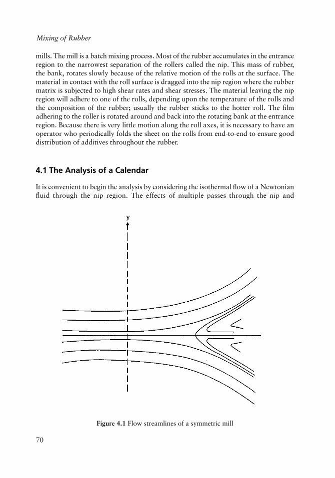
70

Mixing of Rubber

mills. The mill is a batch mixing process. Most of the rubber accumulates in the entrance region to the narrowest separation of the rollers called the nip. This mass of rubber, the bank, rotates slowly because of the relative motion of the rolls at the surface. The material in contact with the roll surface is dragged into the nip region where the rubber matrix is subjected to high shear rates and shear stresses. The material leaving the nip region will adhere to one of the rolls, depending upon the temperature of the rolls and the composition of the rubber; usually the rubber sticks to the hotter roll. The fi lm adhering to the roller is rotated around and back into the rotating bank at the entrance region. Because there is very little motion along the roll axes, it is necessary to have an operator who periodically folds the sheet on the rolls from end-to-end to ensure good distribution of additives throughout the rubber.

4.1 The Analysis of a Calendar

It is convenient to begin the analysis by considering the isothermal fl ow of a Newtonian fl uid through the nip region. The effects of multiple passes through the nip and

Figure 4.1 Flow streamlines of a symmetric mill

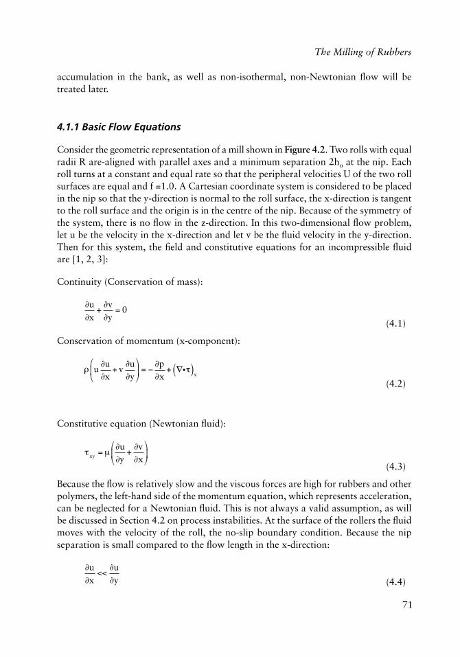
71


accumulation in the bank, as well as non-isothermal, non-Newtonian fl ow will be treated later.

4.1.1 Basic Flow Equations

Consider the geometric representation of a mill shown in Figure 4.2. Two rolls with equal radii R are-aligned with parallel axes and a minimum separation 2ho at the nip. Each roll turns at a constant and equal rate so that the peripheral velocities U of the two roll surfaces are equal and f =1.0. A Cartesian coordinate system is considered to be placed in the nip so that the y-direction is normal to the roll surface, the x-direction is tangent to the roll surface and the origin is in the centre of the nip. Because of the symmetry of the system, there is no fl ow in the z-direction. In this two-dimensional fl ow problem, let u be the velocity in the x-direction and let v be the fl uid velocity in the y-direction. Then for this system, the fi eld and constitutive equations for an incompressible fl uid are [1, 2, 3]:

Continuity (Conservation of mass):

�u�x

+�v�y

= 0

(4.1)

Conservation of momentum (x-component):

� u

�u�x

+ v�u�y

�

��

�

� = �

�p�x

+ �i�( )x

(4.2)

Constitutive equation (Newtonian fl uid):

�xy =�

�u�y

+�v�x

�

��

�

��

(4.3)

Because the fl ow is relatively slow and the viscous forces are high for rubbers and other polymers, the left-hand side of the momentum equation, which represents acceleration, can be neglected for a Newtonian fl uid. This is not always a valid assumption, as will be discussed in Section 4.2 on process instabilities. At the surface of the rollers the fl uid moves with the velocity of the roll, the no-slip boundary condition. Because the nip separation is small compared to the fl ow length in the x-direction:

�u�x

<<�u�y (4.4)

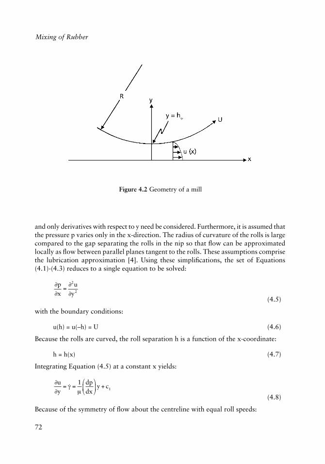
72

Mixing of Rubber

and only derivatives with respect to y need be considered. Furthermore, it is assumed that the pressure p varies only in the x-direction. The radius of curvature of the rolls is large compared to the gap separating the rolls in the nip so that fl ow can be approximated locally as fl ow between parallel planes tangent to the rolls. These assumptions comprise the lubrication approximation [4]. Using these simplifi cations, the set of Equations (4.1)-(4.3) reduces to a single equation to be solved:

�p�x

=�2u�y2

(4.5)

with the boundary conditions:

u(h) = u(–h) = U (4.6)

Because the rolls are curved, the roll separation h is a function of the x-coordinate:

h = h(x) (4.7)

Integrating Equation (4.5) at a constant x yields:

�u�y

= �� =1�

dpdx

�

��

�

��y + c1

(4.8)

Because of the symmetry of fl ow about the centreline with equal roll speeds:

Figure 4.2 Geometry of a mill

73


�u�y y=0

= �� 0( ) = 0

(4.9)

c1 = 0 (4.10)

and

�u�y

=1�

dpdx

�

��

�

��y

(4.11)

Integrating a second time yields:

u =

12�

dpdx

�

��

�

��y2 + c2

(4.12)

At the roll surface where y = h:

U(h) = = U (4.13)

c2 = U

12�

dpdx

�

��

�

��h2

(4.14)

u = U +

y2 g2

2�dpdx

�

��

�

��

(4.15)

The volumetric fl ow rate through the rolls per unit width is calculated:

Q = 2 u(y)dy

0

h

� (4.16)

Substituting Equation (4.15) for the velocity yields:

Q = 2 U +y2 � h2

2�

�

��

�

��dpdx

�

��

�

��dy

0

h

�

= 2h U �h2

3�dpdx

�

��

�

��

(4.17)

Solving this equation for the pressure gradient yields:

dpdx

=3�Uh2

1h1

h

�

��

�

��

(4.18)

74

Mixing of Rubber

where the substitution has been made:

h1 = Q/2U (4.19)

Substituting Equation (4.18) back into (4.15) yields:

u =

U2

3y2

h21

h1

h

�

��

�

�� 1+

3h1

h

�

��

�

��

(4.20)

Now it is convenient to introduce dimensionless variables and to incorporate surface geometry. At the roll surface:

y = ±h

= ± ho + R R x( )1/2( )= ± ho +

x2

2R

�

��

�

��

(4.21)

when x/R is small.

Let dimensionless coordinates be defi ned as:

" = y/(2Rho)1/2 (4.22)

and

# = x/(2Rho)1/2 (4.23)

Use the dimensionless auxiliary variables:

� = (2ho/R)1/2 (4.24)

and

#1 = h1/(2Rho)1/2

= Q/2U(2Rho)1/2 (4.25)

Substituting these dimensionless variables into the expression for the pressure gradient, Equation (4.18), yields:

dpd�

=6�Uho

�

� �12

1+ �2( )3

�

�

��

�

�

��

(4.26)

This equation may be integrated to yield:

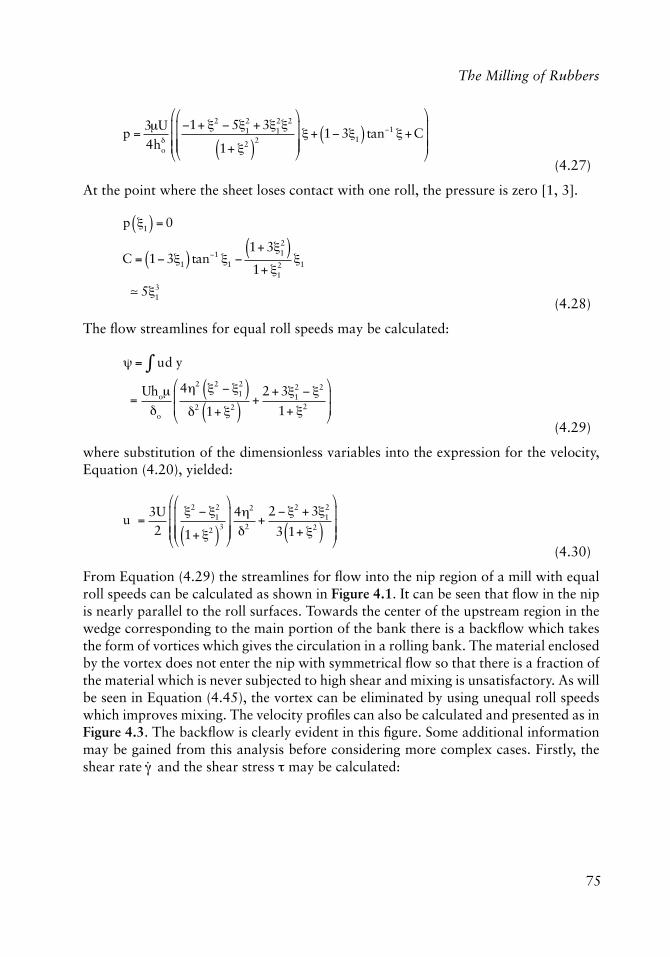
75


p =3�U4ho

�

1+ �2 5�12 + 3�1

2�2

1+ �2( )2

�

�

��

�

�

��+ 1 3�1( ) tan1 �+C

�

�

��

�

�

��

(4.27)

At the point where the sheet loses contact with one roll, the pressure is zero [1, 3].

p �1( ) = 0

C = 1 3�1( ) tan1 �1 1+ 3�1

2( )1+ �1

2�1

� 5�13

(4.28)

The fl ow streamlines for equal roll speeds may be calculated:

� = ud y�

=Uho�

�o

4�2 �2 � �12( )

�2 1+ �2( )+

2 + 3�12 � �2

1+ �2

�

�

�

(4.29)

where substitution of the dimensionless variables into the expression for the velocity, Equation (4.20), yielded:

u =3U2

�2 �12

1+ �2( )3

�

�

�

��

4�2

�2+

2 �2 + 3�12

3 1+ �2( )

�

�

��

�

(4.30)

From Equation (4.29) the streamlines for fl ow into the nip region of a mill with equal roll speeds can be calculated as shown in Figure 4.1. It can be seen that fl ow in the nip is nearly parallel to the roll surfaces. Towards the center of the upstream region in the wedge corresponding to the main portion of the bank there is a backfl ow which takes the form of vortices which gives the circulation in a rolling bank. The material enclosed by the vortex does not enter the nip with symmetrical fl ow so that there is a fraction of the material which is never subjected to high shear and mixing is unsatisfactory. As will be seen in Equation (4.45), the vortex can be eliminated by using unequal roll speeds which improves mixing. The velocity profi les can also be calculated and presented as in Figure 4.3. The backfl ow is clearly evident in this fi gure. Some additional information may be gained from this analysis before considering more complex cases. Firstly, the shear rate

�� and the shear stress � may be calculated:

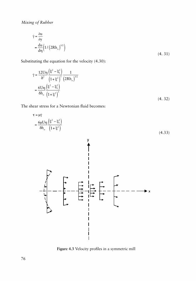
76

Mixing of Rubber

�� =�u�y

=dud�

1 / 2Rho( )1/2( ) (4. 31)

Substituting the equation for the velocity (4.30):

�� =12U��2

�2 �12( )

1+ �2( )3

1

2Rho( )1/2

=6U��ho

�2 �12( )

1+ �2( )3

(4. 32)

The shear stress for a Newtonian fl uid becomes:

� =��

=6�U��ho

�2 �12( )

1+ �2( ) (4.33)

Figure 4.3 Velocity profi les in a symmetric mill

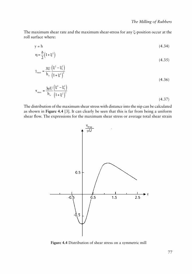
77


The maximum shear rate and the maximum shear-stress for any $-position occur at the roll surface where:

y = h (4.34)

� =

�2

1+ �2( ) (4.35)

��max =3Uho

�2 �12( )

1+ �2( )2

(4.36)

max =3�Uho

�2 �12( )

1+ �2( )2

(4.37)

The distribution of the maximum shear stress with distance into the nip can be calculated as shown in Figure 4.4 [3]. It can clearly be seen that this is far from being a uniform shear fl ow. The expressions for the maximum shear stress or average total shear strain

Figure 4.4 Distribution of shear stress on a symmetric mill

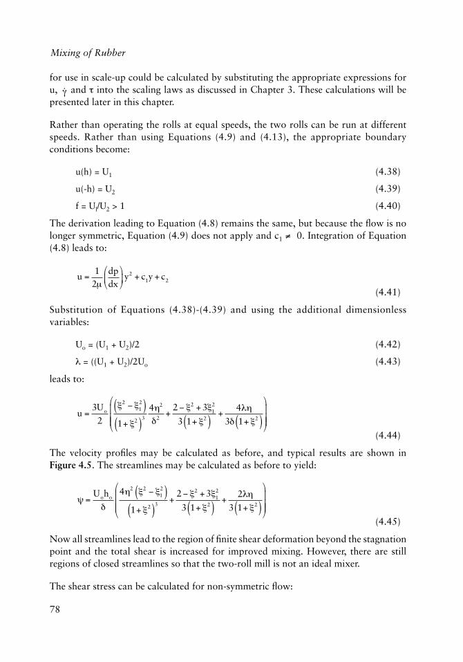
78

Mixing of Rubber

for use in scale-up could be calculated by substituting the appropriate expressions for u,

�� and � into the scaling laws as discussed in Chapter 3. These calculations will be

presented later in this chapter.

Rather than operating the rolls at equal speeds, the two rolls can be run at different speeds. Rather than using Equations (4.9) and (4.13), the appropriate boundary conditions become:

u(h) = U1 (4.38)

u(-h) = U2 (4.39)

f = Ul/U2 > 1 (4.40)

The derivation leading to Equation (4.8) remains the same, but because the fl ow is no longer symmetric, Equation (4.9) does not apply and c1 � 0. Integration of Equation (4.8) leads to:

u =

12�

dpdx

�

��

�

��y2 + c1y + c2

(4.41)

Substitution of Equations (4.38)-(4.39) and using the additional dimensionless variables:

Uo = (U1 + U2)/2 (4.42)

% = ((U1 + U2)/2Uo (4.43)

leads to:

u =3Uo

2

�2 �12( )

1+ �2( )3

4�2

�2+

2 �2 + 3�12

3 1+ �2( )+

4��

3� 1+ �2( )

�

�

��

��

(4.44)

The velocity profi les may be calculated as before, and typical results are shown in Figure 4.5. The streamlines may be calculated as before to yield:

� =Uoho

�

4�2 �2 �12( )

1+ �2( )3

+2 �2 +3�1

2

3 1+ �2( )+

2��

3 1+ �2( )

�

�

��

(4.45)

Now all streamlines lead to the region of fi nite shear deformation beyond the stagnation point and the total shear is increased for improved mixing. However, there are still regions of closed streamlines so that the two-roll mill is not an ideal mixer.

The shear stress can be calculated for non-symmetric fl ow:

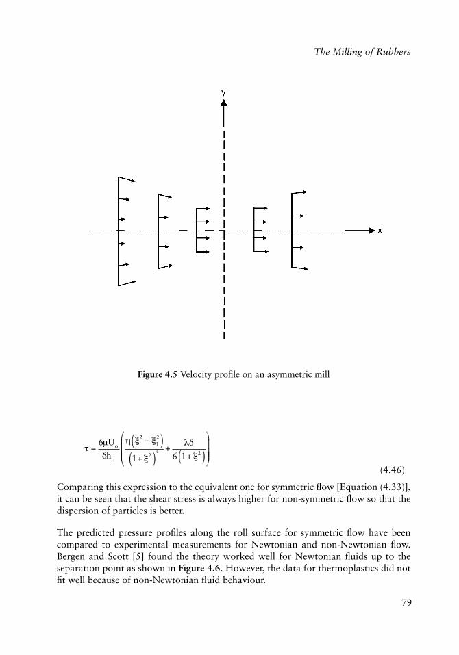
79


� =6�Uo

�ho

� �2 �12( )

1+ �2( )3

+��

6 1+ �2( )

�

�

��

(4.46)

Comparing this expression to the equivalent one for symmetric fl ow [Equation (4.33)], it can be seen that the shear stress is always higher for non-symmetric fl ow so that the dispersion of particles is better.

The predicted pressure profi les along the roll surface for symmetric fl ow have been compared to experimental measurements for Newtonian and non-Newtonian fl ow. Bergen and Scott [5] found the theory worked well for Newtonian fl uids up to the separation point as shown in Figure 4.6. However, the data for thermoplastics did not fi t well because of non-Newtonian fl uid behaviour.

Figure 4.5 Velocity profi le on an asymmetric mill

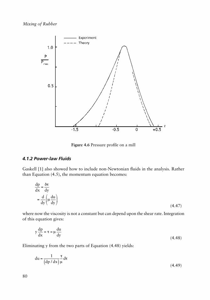
80

Mixing of Rubber

4.1.2 Power-law Fluids

Gaskell [1] also showed how to include non-Newtonian fl uids in the analysis. Rather than Equation (4.5), the momentum equation becomes:

dpdx

=��dy

=ddy

�dudy

�

��

�

��

(4.47)

where now the viscosity is not a constant but can depend upon the shear rate. Integration of this equation gives:

y

dpdx

= � =�dudy

(4.48)

Eliminating y from the two parts of Equation (4.48) yields:

du =1

dp / dx( )��

d�

(4.49)

Figure 4.6 Pressure profi le on a mill

81


Integrating this expression:

u = U �1

dp / dx( )��

�

��

��d�

�

�w

� (4.50)

The volumetric fl ow can be calculated [Equation (4.16)] as:

Q =2

dp / dx( )�d �

0

�w

�

and substituting Equation (4.50):

Q =2U

dp / dx�w �

2U

dp / dx( )2

��

�

��

��d �

�

�w

� d �0

�w

� (4.51)

From Equation (4.48), the shear stress at the wall is:

�w =

dpdx

ho 1+ �2( ) (4.52)

where:

y = h = ho(1+#2)

Substituting into Equation (4.51):

Q = 2Uho 1+ �2( ) � 2

dp / dx( )2

��

�

��

�

�w

�0

�w

� d� d�

(4.53)

Also:

Q = 2Uho 1+ �1

2( ) (4.54)

so that Equation (4.53) becomes:

�2 � �12 =

1

Uho dp / dx( )2

��

�

��

�

�w

�0

�w

� d� d�

(4.55)

which is equivalent to:

�2 � �12 =

1Uho dp / dx( )

�2

�0

�w

� d�

(4.56)

82

Mixing of Rubber

If the material behaves as a power-law fl uid:

� = �o

��o

n1( )/n

(4.57)

then substitution into Equation (4.56) yields:

�2 �12 =

±n�o(n1)/n

2n +1( ) Uho�o dp / dx( )2�w

2n+1( )/n

(4.58)

where the negative sign applies when �12 > �2

. Combining Equations (4.52) and (4.58) and solving for the pressure gradient yields:

dpd�

=k �2 �1

2( )n

1+ �2( )2n+1

�2 > �12

(4.59a)

=k �1

2 �2( )n

1+ �2( )2n+1

�12 > �2

(4. 59b)

where:

k =

2n +1n

�

��

�

��

nU�o

ho�o

�

��

�

��

n�o

ho (4.60)

Comparing the expression for a Newtonian fl uid [Equation (4.26)] to that for a power-law fl uid [Equation (4.60)] where n < 1, the pressure gradient is everywhere lower for non-Newtonian fl ow. Often the pressure for a pseudoplastic fl uid may be only 5-10% of that with a Newtonian fl uid having the same zero-shear-rate viscosity. As a consequence the shear stress will be signifi cantly lower and particle dispersion will not be as effective with a power-law fl uid.

So far only the shear component of fl ow has been considered. As part of the lubrication approximation used in deriving the expressions for velocity, it was assumed that the rate of elongation was small compared to the shear rate:

�u�x

<<�u�y

(4.61)

Using the expression for the velocity from Equation (4.30), the velocity gradients may be calculated for a symmetric mill:

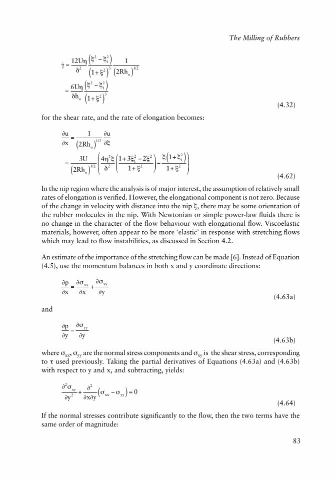
83


�� =12U��2

�2 �12( )

1+ �2( )3

1

2Rho( )1/2

=6U��ho

�2 �12( )

1+ �2( )3

(4.32)

for the shear rate, and the rate of elongation becomes:

�u�x

=1

2Rho( )1/2

�u��

=3U

2Rho( )1/2

4�2�

�2

1+ 3�12 �2�2

1+ �2

�

�

��

� 1+ �12( )

1+ �2

�

�

�

��

(4.62)

In the nip region where the analysis is of major interest, the assumption of relatively small rates of elongation is verifi ed. However, the elongational component is not zero. Because of the change in velocity with distance into the nip #, there may be some orientation of the rubber molecules in the nip. With Newtonian or simple power-law fl uids there is no change in the character of the fl ow behaviour with elongational fl ow. Viscoelastic materials, however, often appear to be more ‘elastic’ in response with stretching fl ows which may lead to fl ow instabilities, as discussed in Section 4.2.

An estimate of the importance of the stretching fl ow can be made [6]. Instead of Equation (4.5), use the momentum balances in both x and y coordinate directions:

�p�x

=��xx

�x+��xy

�y (4.63a)

and

�p�y

=��yy

�y (4.63b)

where xx, yy are the normal stress components and xy is the shear stress, corresponding to � used previously. Taking the partial derivatives of Equations (4.63a) and (4.63b) with respect to y and x, and subtracting, yields:

�2�xy

�y2+

�2

�x�y�xx �� yy( ) = 0

(4.64)

If the normal stresses contribute signifi cantly to the fl ow, then the two terms have the same order of magnitude:

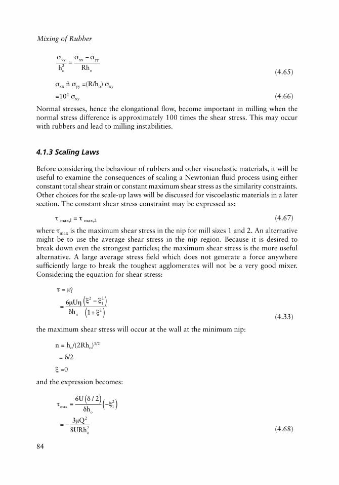
84

Mixing of Rubber

�xy

ho2��xx � yy

Rho (4.65)

xx ñ yy =(R/ho) xy

=102 xy (4.66)

Normal stresses, hence the elongational fl ow, become important in milling when the normal stress difference is approximately 100 times the shear stress. This may occur with rubbers and lead to milling instabilities.

4.1.3 Scaling Laws

Before considering the behaviour of rubbers and other viscoelastic materials, it will be useful to examine the consequences of scaling a Newtonian fl uid process using either constant total shear strain or constant maximum shear stress as the similarity constraints. Other choices for the scale-up laws will be discussed for viscoelastic materials in a later section. The constant shear stress constraint may be expressed as:

� max,l = � max,2 (4.67)

where �max is the maximum shear stress in the nip for mill sizes 1 and 2. An alternative might be to use the average shear stress in the nip region. Because it is desired to break down even the strongest particles; the maximum shear stress is the more useful alternative. A large average stress fi eld which does not generate a force anywhere suffi ciently large to break the toughest agglomerates will not be a very good mixer. Considering the equation for shear stress:

� =��

=6�U��ho

�2 �12( )

1+ �2( ) (4.33)

the maximum shear stress will occur at the wall at the minimum nip:

n = ho/(2Rho)1/2

= �/2

# =0

and the expression becomes:

�max =6U � / 2( )

�ho

�12( )

= 3�Q2

8URho2 (4.68)

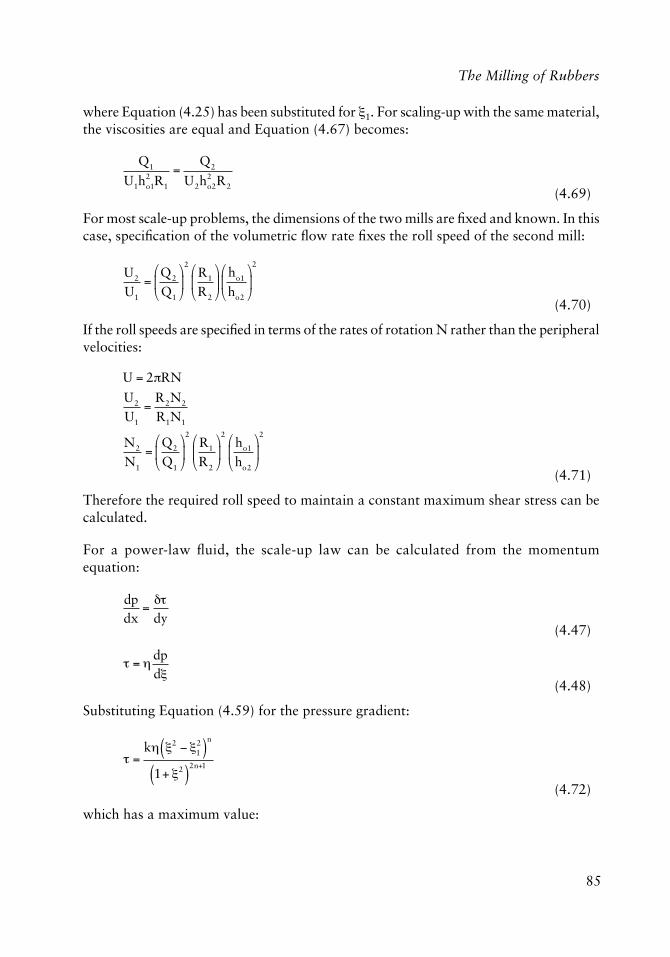
85


where Equation (4.25) has been substituted for #1. For scaling-up with the same material, the viscosities are equal and Equation (4.67) becomes:

Q1

U1ho21R1

=Q2

U2ho2

2R2 (4.69)

For most scale-up problems, the dimensions of the two mills are fi xed and known. In this case, specifi cation of the volumetric fl ow rate fi xes the roll speed of the second mill:

U2

U1

=Q2

Q1

�

��

�

��

2R1

R2

�

��

�

��

ho1

ho2

�

��

�

��

2

(4.70)

If the roll speeds are specifi ed in terms of the rates of rotation N rather than the peripheral velocities:

U = 2�RN

U2

U1

=R2N2

R1N1

N2

N1

=Q2

Q1

�

��

�

��

2R1

R2

�

��

�

��

2ho1

ho2

�

��

�

��

2

(4.71)

Therefore the required roll speed to maintain a constant maximum shear stress can be calculated.

For a power-law fl uid, the scale-up law can be calculated from the momentum equation:

dpdx

=��

dy (4.47)

� = �

dpd�

(4.48)

Substituting Equation (4.59) for the pressure gradient:

� =k� �2 �1

2( )n

1+ �2( )2n+1

(4.72)

which has a maximum value:

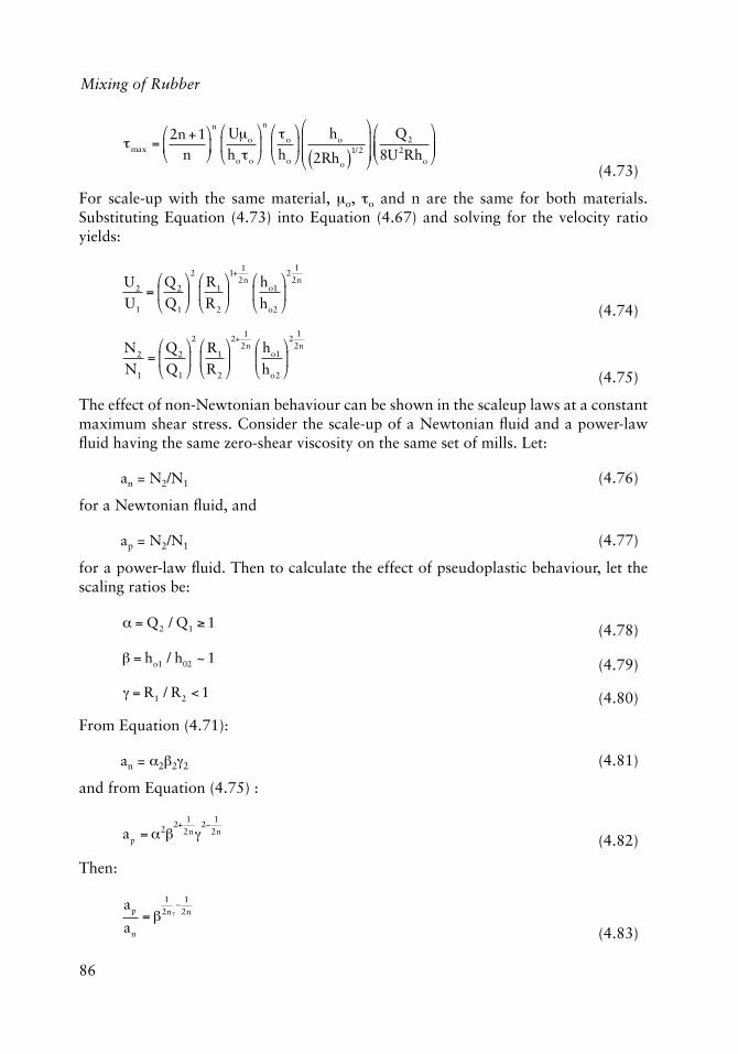
86

Mixing of Rubber

�max =2n +1

n

�

��

�

��

nU�o

ho�o

�

��

�

��

n�o

ho

�

��

�

��

ho

2Rho( )1/2

�

�

��

�

�

��

Q2

8U2Rho

�

��

�

��

(4.73)

For scale-up with the same material, �o, �o and n are the same for both materials. Substituting Equation (4.73) into Equation (4.67) and solving for the velocity ratio yields:

U2

U1

=Q2

Q1

�

��

�

��

2R1

R2

�

��

�

��

1+1

2n ho1

ho2

�

��

�

��

21

2n

(4.74)

N2

N1

=Q2

Q1

�

��

�

��

2R1

R2

�

��

�

��

2+1

2n ho1

ho2

�

��

�

��

21

2n

(4.75)

The effect of non-Newtonian behaviour can be shown in the scaleup laws at a constant maximum shear stress. Consider the scale-up of a Newtonian fl uid and a power-law fl uid having the same zero-shear viscosity on the same set of mills. Let:

an = N2/N1 (4.76)

for a Newtonian fl uid, and

ap = N2/N1 (4.77)

for a power-law fl uid. Then to calculate the effect of pseudoplastic behaviour, let the scaling ratios be:

� = Q2 / Q1 �1 (4.78)

� = ho1 / h02 ~ 1 (4.79)

� = R1 / R2 < 1 (4.80)

From Equation (4.71):

an = �2&2�2 (4.81)

and from Equation (4.75) :

ap = �2�

2+1

2n�2

12n

(4.82)

Then:

ap

an

= �1

2n �

12n

(4.83)

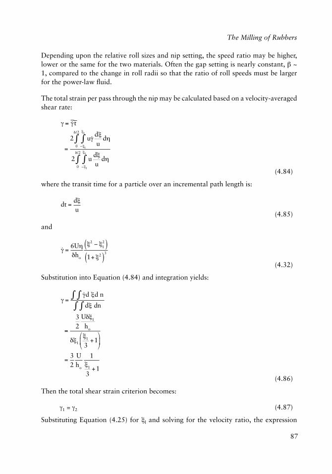
87


Depending upon the relative roll sizes and nip setting, the speed ratio may be higher, lower or the same for the two materials. Often the gap setting is nearly constant, & ~ 1, compared to the change in roll radii so that the ratio of roll speeds must be larger for the power-law fl uid.

The total strain per pass through the nip may be calculated based on a velocity-averaged shear rate:

� = ��t

=

2 u��d�u

d��1

�1

�0

� /2

�

2 ud�u

d��1

�1

�0

�/2

� (4.84)

where the transit time for a particle over an incremental path length is:

dt =

d�u

(4.85)

and

�� =6U��ho

�2 �12( )

1+ �2( )3

(4.32)

Substitution into Equation (4.84) and integration yields:

� =��d �d n��d� dn��

=

32

U��1

ho

��1

�1

3+1

�

��

�

=32

Uho

1�1

3+1

(4.86)

Then the total shear strain criterion becomes:

�1 = �2 (4.87)

Substituting Equation (4.25) for #l and solving for the velocity ratio, the expression

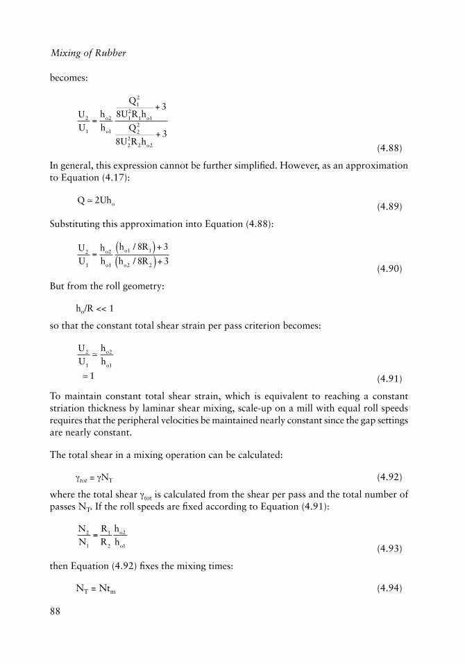
88

Mixing of Rubber

becomes:

U2

U1

=ho2

ho1

Q12

8U12R1ho1

+ 3

Q22

8U22R2ho2

+ 3

(4.88)

In general, this expression cannot be further simplifi ed. However, as an approximation to Equation (4.17):

Q � 2Uho (4.89)

Substituting this approximation into Equation (4.88):

U2

U1

=ho2

ho1

ho1 / 8R1( ) + 3

ho2 / 8R2( )+ 3 (4.90)

But from the roll geometry:

ho/R << 1

so that the constant total shear strain per pass criterion becomes:

U2

U1

�ho2

ho1

� 1 (4.91)

To maintain constant total shear strain, which is equivalent to reaching a constant striation thickness by laminar shear mixing, scale-up on a mill with equal roll speeds requires that the peripheral velocities be maintained nearly constant since the gap settings are nearly constant.

The total shear in a mixing operation can be calculated:

�tot = �NT (4.92)

where the total shear �tot is calculated from the shear per pass and the total number of passes NT. If the roll speeds are fi xed according to Equation (4.91):

N2

N1

=R1

R2

ho2

ho1 (4.93)

then Equation (4.92) fi xes the mixing times:

NT = Ntm (4.94)

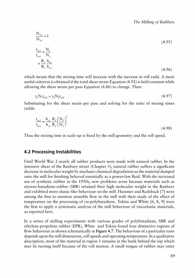
89


NT2

NT1

= 1

(4.95)

tm2

tm1

=N1

N2

=R2

R1

h01

ho2 (4.96)

which means that the mixing time will increase with the increase in roll radii. A more useful criterion is obtained if the total shear strain Equation (4.92) is held constant while allowing the shear strain per pass Equation (4.86) to change. Then:

�1N1tm1 = �2N2tm2 (4.97)

Substituting for the shear strain per pass and solving for the ratio of mixing times yields:

tm2

tm1

=ho2

ho1

R1

R2

N1

N2

�

��

�

��

2

(4.98)

Thus the mixing time in scale-up is fi xed by the mill geometry and the roll speed.

4.2 Processing Instabilities

Until World War 2 nearly all rubber products were made with natural rubber. In the intensive shear of the Banbury mixer (Chapter 5), natural rubber suffers a signifi cant decrease in molecular weight by mechano-chemical degradation so the material dumped onto the mill for fi nishing behaved essentially as a power-law fl uid. With the increased use of synthetic rubber in the 1950s, new problems arose because materials such as styrene-butadiene-rubber (SBR) retained their high molecular weight in the Banbury and exhibited more elastic-like behaviour on the mill. Hammer and Railsback [7] were among the fi rst to mention unstable fl ow in the mill with their study of the effect of temperature on the processing of cis-polybutadiene. Tokita and White [6, 8, 9] were the fi rst to apply a systematic analysis of the mill behaviour of viscoelastic materials, as reported here.

In a series of milling experiments with various grades of polybutadiene, SBR and ethylene-propylene rubber (EPR), White and Tokita found four distinctive regions of fl ow behaviour as shown schematically in Figure 4.7. The behaviour of a particular resin depends upon the mill dimensions, roll speeds and operating temperature. In a qualitative description, most of the material in region 1 remains in the bank behind the nip which may be turning itself because of the roll motion. A small tongue of rubber may enter

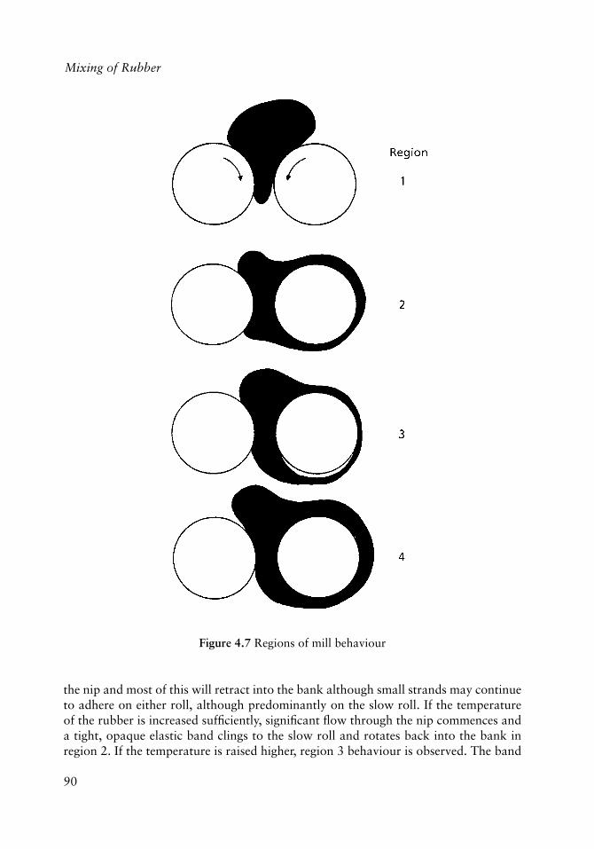
90

Mixing of Rubber

the nip and most of this will retract into the bank although small strands may continue to adhere on either roll, although predominantly on the slow roll. If the temperature of the rubber is increased suffi ciently, signifi cant fl ow through the nip commences and a tight, opaque elastic band clings to the slow roll and rotates back into the bank in region 2. If the temperature is raised higher, region 3 behaviour is observed. The band

Figure 4.7 Regions of mill behaviour

91


becomes transparent and may sag from the roll surface in mild bagging. In some cases bagging begins on the opaque material. The bag may crumble or tear, depending upon the material and operating conditions. If the temperature is increased again, region 4 behaviour is observed where a transparent, viscoelastic fl uid fl ows through the nip and usually adheres to the slow roll. At higher roll speeds, ripples may appear because of pressure-viscous effects leading to instability [10].

In region 1 there is essentially no fl ow between the rolls. Consequently the analysis used before is not applicable in this region. Instead consider the behaviour of the rubber sitting in the mill bank [11]. The material adjacent to the roll surface will try to adhere to it. Because the rolls rotate a stress is generated and transmitted through the rubber, The material will fl ow in response to the applied stress so that this is a complex creep problem. As the material dragged by the rolls enters the nip region, resistance to fl ow increases and the shear stress at the wall must increase for the fl ow to continue. The strength of the forces attaching the rubber to the roll surface has a fi nite value. If the shear forces exceed the critical value corresponding to the force of adhesion, the wall will move relative to the rubber. When slip occurs, the rubber will not enter the nip and an oscillating tongue is observed as material slips and sticks to the wall. There are complex fl ow patterns because of circulation in the bank which preclude an analytical solution but the essential behaviour can be predicted from the following analysis.

If the wall shear stress exceeds the critical stress, there is no fl ow through the nip. Below the critical stress, fl ow occurs essentially as described before with appropriate changes for a viscoelastic fl uid. At the critical operating conditions:

�w = crit (4.99)

If the fl ow can be treated as a one-dimensional creep problem:

�(t) = J(t) crit (4.100)

where the strain � is related to the critical stress by the dependent creep compliance J(t). If the fl uid behaviour can be approximated by linear viscoelasticity, the creep compliance and the shear modulus are related by the convolution integral [12]:

J(t � s)G(s)ds = 1 / t

0

t

� (4.101)

The simplest viscoelastic model which exhibits the essential behaviour is the Maxwell model for which:

G(t) = Go exp(-t/%) (4.102)

where the modulus is related to the initial modulus Go and the relaxation time %. The fl uid viscosity is given by:

92

Mixing of Rubber

� = %Go (4.103)

This is the deformation behaviour which would be observed for a mechanical analogue which consists of a spring and viscous dashpot in series.

Substituting Equation (4.103) into the convolution integral and solving for the compliance:

J(t) =1

Go

+t�

=1

Go

+t

�Go (4.104)

The time required for material to pass through the mill is essentially that required to obtain a shear strain:

� = R/ho (4.105)

Substituting Equations (4.104) and (4.105) into the creep equation, the critical fl ow time can be calculated:

tcrit = �Rho

�

��

�

��

Go

� crit

�

��

�

�� 1

�

��

�

��

(4.106)

The approximate transit time for a fl uid element at the roll surface is:

t = ho/�RN (4.107)

If this value is less than tcrit then region 1 behaviour will be observed, which is equivalent to too rapid a rate of roll rotation.

Most rubbers are not described properly by a single Maxwell element but their behaviour may be described by a parallel array of elements, each with their own characteristic retardation time [12] If this distribution of retardation times is continuous, then the epxression for the creep compliance becomes:

J(t) = L(�) 1� exp �t / �( )( )d�n� + t / �( )

��

+�

� (4.108)

where L(%) is the spectrum of retardation times. Substituting this expression into the creep equation yields an implicit expression for the critical time for fl ow through the nip:

Rho

= � crit L(�) 1� exp �t / �( )( )d�n� +t� crit

��

+�

� (4.109)

93


The response of a viscoelastic material depends upon the time scale of the experiment compared to the relaxation time of the material. Silly putty is a familiar example of this phenomenon. If a ball is formed from this silicone rubber and dropped onto the fl oor, it bounces because the time of impact, on the order of milliseconds, is small compared to the relaxation time of the material, on the order of seconds.

If the ball is left on a table, it will fl ow into a pool within an hour because of the pull of gravity. The time of the experiment is long compared to the relaxation time and the material behaves as a fl uid rather than an elastic solid.

This dependence of the fl ow behaviour on the ratio of the time scale of an experiment to the material relaxation time can explain the appearance of region 1. The time scale of the experiment may be expressed as the ratio of a characteristic length to the roll velocity. Because we are concerned with fl ow through the nip, the roll gap (2ho) and roll velocity (2�RN) are the appropriate values, resulting in Equation (4.107). Substituting into Equation (4.106), a Weissenberg number (We) may be calculated:

We = � / t

=��RN

ho

=Rho

�

��

�

�

Go crit

�

��

�

� �1

�

��

�

�

�1

(4.110)

For values much less than unity, the material behaves as a viscous fl uid; for values greater than unity, the material behaves elastically. For values near one, the behaviour is highly complex.

The change in the Weissenberg number with operating conditions and material qualitatively explains the region 1 - region 2 transition observed by Tokita and White. For the same material and operating temperature, an increase in gap half-width (ho) decreases the Weissenberg number. Flow was observed to become more stable when this happened and the transition to region 2 occurred. For a constant mill geometry, increasing the temperature decreases the relaxation time. This lowers the Weissenberg number and again transition to stable region 2 was observed.

Because of the approximate nature of the analysis of region 1 behaviour, the equations cannot be directly applied to process design. Two important points do arise from the analysis. Firstly, there is a characteristic number, the Weissenberg number, which is a measure of how the material will respond in the mill. In scale-up, this will prove to be an important group. Secondly, this analysis gives a qualitative understanding of the causes of stop-start instability in a rubber mill. This oscillating fl ow arises from the viscoelastic nature of the rubber. In practice, the problem may be overcome by increasing the nip gap, decreasing the roll speed or raising the temperature. In the next chapter on internal

94

Mixing of Rubber

mixers, it will be seen that this instability may delay the start of effective mixing cycles as well as limiting the maximum shear stress by preventing fl ow between the rotor tip and chamber wall.

Milling in region 2 consists of a tight elastic band clinging to one roll. In this region the material exhibits its full viscoelastic behaviour. As the roll speed increases, minute tears and surface irregularities form which heal within one revolution. A decrease in nip gap leads to a smoother, tight band. If the band is cut, the rubber will retract from the hole because of stored elastic energy.

The full viscoelastic problem is not amenable to solution, even for relatively simple viscoelastic constitutive equations. Despite this lack of analysis, some information can be obtained for this region. The lower temperature limits and operating conditions are set by the transition to region 1 behaviour just described. In region 2 surface irregularities and tears form on the band surface as the material separates from the second roll. In the region of stable operation, the surface tears will not propagate within the time of a single revolution of the roll. The tear will only propagate if the stored energy arising from deformation in the mill nip exceeds a critical value, and the rate of tear propagation is a function of the stored energy [11]. Thus two criteria can be set for the upper limit to a stable region 2. Firstly:

E ' Ecrit (4.111)

where E is the stored elastic energy of a material having a critical tearing energy (Ecrit). Secondly, the stress generated in a single pass, which is a function of the mill geometry and operating conditions, must essentially relax in one revolution of the rolls. If the stress does not relax, the material will become oriented along the fl ow lines and shear mixing will decrease. Furthermore stress will rapidly build up and exceed the critical wall stress so slip begins at the wall. For the stress to relax in one revolution, the relaxation time must be small compared to the period of revolution. The Deborah number (De) is a measure of this ratio:

De = %/trot

= 2�%N (4.112)

In contrast to the Weissenberg number, the only machine parameter is the rate of rotation. In scale-up, the Deborah number should also be kept constant in order to preserve the fl ow regime. Other uses of the Deborah number will be given in Chapter 5. The higher the temperature, the more rapidly stress will relax. The slower the roll speed, the more stable the operation is.

The upper limit for stable operation is set by a stored energy criterion. The stored elastic energy density for a Maxwell fl uid may be calculated:

E = tr T2/2G (4.113)

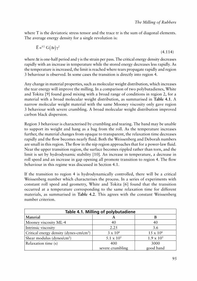
95


where T is the deviatoric stress tensor and the trace tr is the sum of diagonal elements. The average energy density for a single revolution is:

E =1/2 G �t( ) �2

(4.114)

where �t is one-half period and � is the strain per pass. The critical energy density decreases rapidly with an increase in temperature while the stored energy decreases less rapidly. As the temperature is increased, the limit is reached where tears propagate rapidly and region 3 behaviour is observed. In some cases the transition is directly into region 4.

Any change in material properties, such as molecular weight distribution, which increases the tear energy will improve the milling. In a comparison of two polybutadienes, White and Tokita [9] found good mixing with a broad range of conditions in region 2, for a material with a broad molecular weight distribution, as summarised in Table 4.1. A narrow molecular weight material with the same Mooney viscosity only gave region 3 behaviour with severe crumbling. A broad molecular weight distribution improved carbon black dispersion.

Region 3 behaviour is characterised by crumbling and tearing. The band may be unable to support its weight and hang as a bag from the roll. As the temperature increases further, the material changes from opaque to transparent, the relaxation time decreases rapidly and the fl ow becomes nearly fl uid. Both the Weissenberg and Deborah numbers are small in this region. The fl ow in the nip region approaches that for a power-law fl uid. Near the upper transition region, the surface becomes rippled rather than torn, and the limit is set by hydrodynamic stability [10]. An increase in temperature, a decrease in roll speed and an increase in gap opening all promote transition to region 4. The fl ow behaviour in this regime was discussed in Section 4.1.

If the transition to region 4 is hydrodynamically controlled, there will be a critical Weissenberg number which characterises the process. In a series of experiments with constant roll speed and geometry, White and Tokita [6] found that the transition occurred at a temperature corresponding to the same relaxation time for different materials, as summarised in Table 4.2. This agrees with the constant Weissenberg number criterion.

Table 4.1. Milling of polybutadieneMaterial A BMooney viscosity ML-4 40 40Intrinsic viscosity 2.25 3.6Critical energy density (dynes-cm/cm3) 3 x 106 15 x 106

Shear modulus (dynes/cm2) 5.1 x 105 1.9 x 105

Relaxation time (s) 400severe crumbling

3000good band

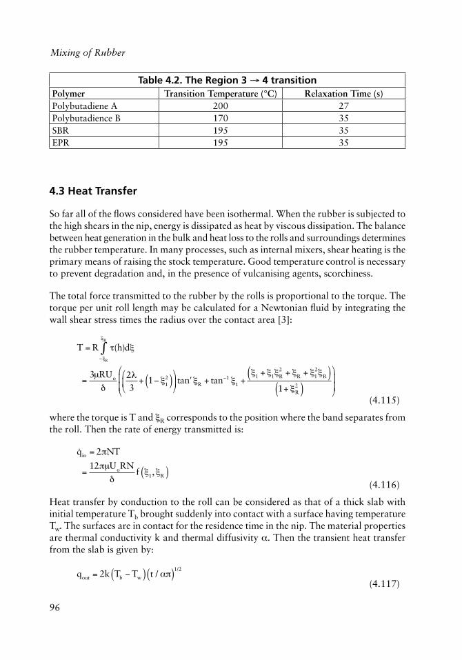
96

Mixing of Rubber

Table 4.2. The Region 3 � 4 transitionPolymer Transition Temperature (°C) Relaxation Time (s)Polybutadiene A 200 27Polybutadience B 170 35SBR 195 35EPR 195 35

4.3 Heat Transfer

So far all of the fl ows considered have been isothermal. When the rubber is subjected to the high shears in the nip, energy is dissipated as heat by viscous dissipation. The balance between heat generation in the bulk and heat loss to the rolls and surroundings determines the rubber temperature. In many processes, such as internal mixers, shear heating is the primary means of raising the stock temperature. Good temperature control is necessary to prevent degradation and, in the presence of vulcanising agents, scorchiness.

The total force transmitted to the rubber by the rolls is proportional to the torque. The torque per unit roll length may be calculated for a Newtonian fl uid by integrating the wall shear stress times the radius over the contact area [3]:

T = R �(h)d��R

�R

�

=3�RUo

�

2�3

+ 1� �12( )

�

�

�ta �n �R + tan�1 �1 +

�1 + �1�R2 + �R + �1

2�R( )1+ �R

2( )�

��

��

(4.115)

where the torque is T and #R corresponds to the position where the band separates from the roll. Then the rate of energy transmitted is:

�qin = 2�NT

=12��UoRN

�f �1,�R( )

(4.116)

Heat transfer by conduction to the roll can be considered as that of a thick slab with initial temperature Tb brought suddenly into contact with a surface having temperature Tw. The surfaces are in contact for the residence time in the nip. The material properties are thermal conductivity k and thermal diffusivity �. Then the transient heat transfer from the slab is given by:

qout = 2k Tb �Tw( ) t / ��( )1/2

(4.117)

97


Then the rate of heat transfer is:

�qout = �k Tb �Tw( ) / ��( )1/2{ }

t�32

(4.118)

At steady-state the rate of energy dissipation equals the rate of heat conduction:

�qin + �qout = 0

(4.119)

Substituting Equations (4.116) and (4.118) into this equation and solving for the bulk temperature yields:

Tb = Tw +

12��R2N1/2 ��( )1/2

�kf �1,�R( )

(4.120)

Thus the rubber temperature will increase with roll surface temperature because of a lower driving force for heat conduction. The temperature will also increase with roll speed and decrease with gap width, both of which raise the shear rate, hence increasing the rate of viscous dissipation.

In deriving this expression, it was assumed that the material properties were independent of temperature. In practice the viscosity is strongly temperature-dependent so that the energy equation and momentum equation are strongly coupled. In this case the equations cannot be solved analytically.

Consider the energy equation for one-dimensional fl ow between parallel plates:

�Cp

�T�t

+ u�T�x

�

��

�

� = k

�2T�y2

+��u�y

�

��

�

�

2

(4.121)

where the Newtonian viscosity has the temperature-dependence:

� = �o exp(–b(T – To)) (4.122)

Choose the following dimensionless variables:

* = b(T – To) (4.123)

V = u/U (4.124)

where:

U = Q/2ho

X = x/L (4.125a)

98

Mixing of Rubber

y = y/h (4.125b)

� = Lt/U (4.126)

Dividing Equation (4.121) by ,c and substituting the dimensionless variables, the energy equation becomes:

Gz

��

+ V��X

�

�

�

�� =

�2�

�Y2+ Gr

�V�Y

�

�

�

��

2

e��

(4.127)

where the dimensionless groups have been extracted:

Gz = Graetz number = (Uh2,c)/kL (4.128)

Gr = Griffi ths number = (�oU2)/k ... (4.129)

The Graetz number is a measure of the rate of heat convection compared to heat conduction and the Griffi th number is a measure of the rate of viscous dissipation compared to the rate of heat conduction. Finally, the dimensionless group *w =b(Tw – To) is a measure of how the temperature-dependence of viscosity affects the fl ow fi eld.

In the case of the two-roll mill, L is the roll radius, the scaling velocity is the peripheral roll speed, h is the nip halfwidth and Tw is the roll surface temperature.

Several distinct cases may be recognised. If the Graetz number is small compared to unity, the convection term is negligible and the temperature fi eld is locally determined. If the Griffi ths number is small as well, dissipation is not important and the fl ow is essentially isothermal. If the Griffi ths number is large, the fl ow becomes adiabatic. If the Graetz number is large and the Griffi ths number is small compared to unity, the fl ow is essentially determined by the upstream temperature; streamlines are isotherms. If the Griffi ths number is of order one, then the energy and momentum equations are rheologically coupled and must be solved simultaneously. In scale-up it is usually desirable to maintain the same temperature history for the process. This will be the case if the Graetz number and Griffi ths number are kept constant in scale-up as well as *w constant.

The analysis for heat transfer with a Newtonian fl uid presented before equated the energy dissipation to the heat conduction. This was equivalent to a large Griffi ths number and a small Graetz number where convection can be neglected.

A simple analysis of heat transfer yields the average temperature. Even when the predicted or measured temperature is reasonable, hot spots may arise in the bulk of the material because of viscous dissipation. If the Griffi ths number is large, this may be an important source of trouble in control and the temperature distribution required can be predicted only by a numerical solution to the fully-coupled momentum and energy equations.

99


4.4 Scale-up Alternatives

A number of alternative scaling rules are possible for calculating the new operating conditions when transferring a process from the laboratory mill to the plant equipment:

l. Simple geometric similarity

2. Constant maximum shear stress

3. Constant total shear strain

4. Constant mixing time

5. Constant stock temperature history

6. Constant Weissenberg/Deborah numbers

7. Constant Graetz/Griffi ths numbers

Most of these criteria refl ect a particular physical process which is believed to control the rate and/or stability of the process. For example, the constant maximum shear stress criterion implies that agglomerate break-up is critical in determining the mixing quality while the constant total strain criterion implies that striation thickness is the crucial quantity. Some of these criteria may be mutually compatible, including the constraints imposed by existing mill geometry, but in other cases the criteria may be incompatible.

In the usual scale-up problem, a trial formulation of material is prepared on a small laboratory mill having a radius (R1) and nip gap (hol) by mixing for time (tl) at a roll speed (N1). The mass temperature increases from room temperature to T1 while the roll surface temperature is kept at Tw1. The material behaves essentially as a Newtonian fl uid (with a temperature-dependent viscosity given in Equation (4.122). The fl ow rate through the nips under these conditions is Q1. The plant mill has a radius (R2) and gap setting (ho2) which is adjustable over a narrow range. The mill speed (N2) and mixing time (t2) are to be selected so that the mixture maintains its quality while processing material at a rate (M2).

One parameter which has not been specifi ed is the size of the bank. This represents a reservoir of material which feeds the nip. If the rubber only made one pass, then the bank size would not matter. However, when the mill is operated as a batch mixer, each element of rubber spends only a fraction of the total mixing time in the nip. If the fl ow rate through the nip is known and the total amount of material on the rolls in M, the quantity to be mixed in time t, then on the average, each element makes P passes through the nip:

100

Mixing of Rubber

P = Qt/M (4.130)

With a given mill, the amount of rubber in the nip and on the roll is essentially constant so that the effect of increasing the bank size is to decrease the number of passes per element if operating conditions are constant. Hence the average production rate M/t is an important variable, especially when the total shear strain, the product of shear strain per pass times the number of passes, is used. The fi rst possible scale-up rule is to keep the ratio of gap separation to roll radius constant for both mills but specifying the roll speed, mixing time or production rate by independent criteria. The geometric constraint is:

R1

ho1

=R2

ho2 (4.131)

The operating variables N2, t2 and M2 cannot be fi xed without three further constraints on the system. In some cases these are provided by external process considerations such as the necessity to process the dump from an internal mixer in the time interval between dumps, which fi xes M2 and t2 The third constraint can be provided by one of the other scaling criteria or by an arbitrary decision such as keeping the roll speed constant or the peripheral roll velocity constant. Without further guidance, the choice is arbitrary. In many commercial mills, the criterion in Equation (4.131) is not met because of limitations in mechanical design and the roll rate of rotation is fi xed or adjustable to a small choice of values. Therefore in general the criterion of geometric similarity is not of use in rubber mills.

The second possible choice of scaling laws is that the maximum shear stress must be maintained constant, as was previously discussed. For a Newtonian fl uid, the results are:

�max =

3�Q2

8URho2

(4.68)

and

N2

N1

=Q2

Q1

�

��

�

��

2�2

�1

�

��

�

��

ho1

ho2

�

��

�

��

2R1

R2

�

��

�

��

(4.132)

where the viscosities may not be equal if the temperature histories are not the same. If the fl ow rate Q is approximated by Equation (4.89), then the roll speed ratio becomes:

N2

N1

=�1

�2 (4.133)

101


Because the viscosity ratio will be nearly unity in scale-up, the constant roll speed criterion often cited can be seen to be equivalent to a maximum shear stress criterion.

If the fl uid behaves as a power-law rather than Newtonian fl uid, the expression then becomes:

N2

N1

=Q2

Q1

�

��

�

��

2R1

R2

�

��

�

��

2+1

2n ho1

ho2

�

��

�

��

21

2n

(4.75)

and with substitution of Equation (4.89):

N2

N1

=R2

R1

�

��

�

��

2nho1

ho2

�

��

�

��

1/2n

(4.134)

In constrast to the case for Newtonian fl uids, the scale-up of power-law fl uids always depends upon the roll geometry. The criterion of maximum shear stress does not explicitly place constraints upon either the temperature or the mixing time for the batch. In the scale-up process, the temperature may not be the same for the two mills. The temperature requirements will be considered shortly, but consider for now that the temperature histories, hence �l and �2, are known. Then to calculate the mixing time, one possibility is to assume that a certain fraction of the particles per unit fl uid volume are broken per pass through the nips. To obtain the same size reduction in scale-up then requires that the number of passes (Equation (4.130)) be held constant:

Q1t1

M1

=Q2t2

M2 (4.135)

Substituting Equation (4.89) yields:

t2

t1

=M2

M1

�

��

�

��

R1

R2

�

��

�

��

N1

N2

�

��

�

��

ho1

ho2

�

��

�

��

(4.136)

and the roll speed ratio is given by Equation (4.133). Thus the mixing time is proportional to the amount of material to be mixed and inversely proportional to the roll size.

If there is an upper temperature limit because of degradation or scorching, then this scaling law might confl ict with the maximum temperature requirement, as discussed below. A less serious limitation on these equations is that unequal roll speeds has been neglected. This effect can be incorporated by using Equations (4.44) and (4.46) as the starting points for an analysis similar to that just presented.

The average shear strain per pass through the nip has been calculated in Equation (4.86). The total shear strain criterion becomes:

102

Mixing of Rubber

�T = �1P1 = �2P2 (4.137)

If the amount of material is the same, then Equation (4.96) results. More generally, this is not the case. Combining Equations (4.86) and (4.130) yields an expression for the mixing time:

t2

t1

=M2

M1

�

��

�

��

N1

N2

�

��

�

��

2R1

R2

�

��

�

��

2

(4.138)

If the mills have strict geometric similarity, then a constant maximum stress criterion can be used to set the ratio of roll speeds and Equations (4.136) and (4.138) yield the same predictions for mixing time. Even when the rolls are not geometrically similar, the two criteria are compatible. This will not be necessarily true for internal mixers.

In the transfer of the process to the larger mill, it is usually desirable to remain in the same fl ow regime, and in particular, it is necessary to avoid regions 1 and 3 where fl ow instabilities occur. The fl ow will be hydrodynamically similar if both the Weissenberg and Deborah numbers are kept constant. The Weissenberg number criterion, from Equation (4.110), becomes:

�1R1N1

ho1

=�2R2N2

ho2 (4.139)

and the Deborah number criterion, from Equation (4.112) becomes:

%1N1 = %2N2 (4.140)

The ratio of roll speeds is fi xed by the Deborah number requirement. If the temperature history is the same for the two mills, then the relaxation time is the same and this criterion becomes the same as for a Newtonian fl uid. In many cases, the ratio of relaxation times equals the ratio of viscosities so the criterion is preserved. The Weissenberg number criterion then fi xes the roll geometry:

R2

R1

=ho2

ho1

which is the requirement of strict geometric similarity. In most cases, this criterion cannot be met. In scale-up, the radius increases while the nip gap is nearly constant. Then scaling at constant Deborah number, or often the same roll speed, increases the Weissenberg number. This can lead to fl ow instability and processing diffi culties in scale-up. If, however, it is decided to keep the Weissenberg number constant and to allow the Deborah number to change:

103


De2

De1

=�2N2

�1N1

=R1

R2

ho2

ho1 (4.141)

The Deborah number will decrease with scale-up at constant Weissenberg number so that the fl ow will remain stable. The roll speeds can be set by solving Equation (4.139):

N2

N1

=ho2

ho1

�

��

�

��

R1

R2

�

��

�

��1

�2

�

��

�

��

(4.142)

and this value used in Equation (4.138) to fi x the mixing time at a constant total shear.

The constant mixing time criterion is not a very useful concept for scale-up. The idea originated from the problem of controlling cycles in an internal mixer, where the constant mixing time criterion can be equivalent to a constant total shear criterion, as discussed in Chapter 5. This is not the case in mills and the mixing time in scale-up is not simply related to any fundamental physical process.

The solution of the coupled energy and momentum equations is very diffi cult, especially for viscoelastic materials. However, if a material has been successfully mixed on a small mill, the temperature history of the material will be the same on a larger mill if the dimensionless energy Equation (4.127) remains unchanged with identical boundary conditions. This will be the case if the Graetz and Griffi ths numbers are held constant and the wall temperatures are the same. The thermal diffusivity is essentially constant so the Graetz number criterion becomes [Equation (4.128)]:

U1h12

R1

=U2h02

2

R2 (4.143)

and the Griffi ths number criterion becomes [Equation (4.129)]:

U1

2 = U22

(4.144)

This fi xes the ratio of roll speeds:

N2

N1

=R1

R2 (4.145)

and the mill geometry:

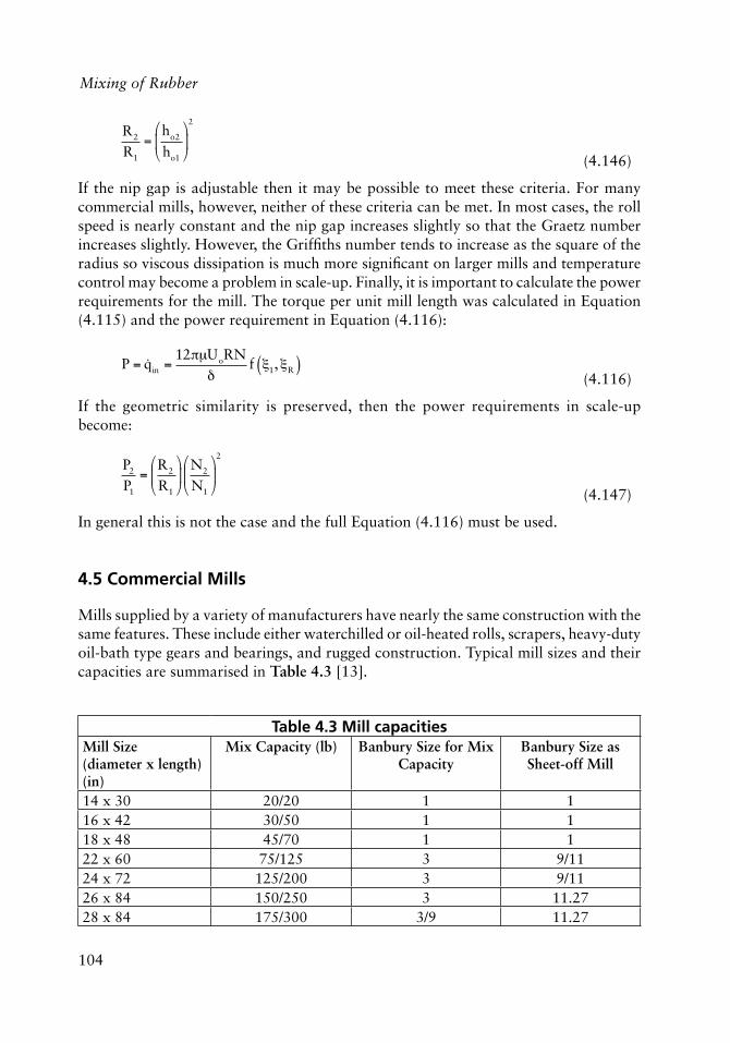
104

Mixing of Rubber

R2

R1

=ho2

ho1

�

��

�

��

2

(4.146)

If the nip gap is adjustable then it may be possible to meet these criteria. For many commercial mills, however, neither of these criteria can be met. In most cases, the roll speed is nearly constant and the nip gap increases slightly so that the Graetz number increases slightly. However, the Griffi ths number tends to increase as the square of the radius so viscous dissipation is much more signifi cant on larger mills and temperature control may become a problem in scale-up. Finally, it is important to calculate the power requirements for the mill. The torque per unit mill length was calculated in Equation (4.115) and the power requirement in Equation (4.116):

P = �qin =

12��UoRN�

f �1,�R( ) (4.116)

If the geometric similarity is preserved, then the power requirements in scale-up become:

P2

P1

=R2

R1

�

��

�

��

N2

N1

�

��

�

��

2

(4.147)

In general this is not the case and the full Equation (4.116) must be used.

4.5 Commercial Mills

Mills supplied by a variety of manufacturers have nearly the same construction with the same features. These include either waterchilled or oil-heated rolls, scrapers, heavy-duty oil-bath type gears and bearings, and rugged construction. Typical mill sizes and their capacities are summarised in Table 4.3 [13].

Table 4.3 Mill capacitiesMill Size (diameter x length) (in)

Mix Capacity (lb) Banbury Size for Mix Capacity

Banbury Size as Sheet-off Mill

14 x 30 20/20 1 116 x 42 30/50 1 118 x 48 45/70 1 122 x 60 75/125 3 9/1124 x 72 125/200 3 9/1126 x 84 150/250 3 11.2728 x 84 175/300 3/9 11.27

105


4.6 Summary

In this chapter, considerable attention has been given to obtaining analytical solutions to the problem of fl ow in a two-roll mill. Following an outline of the solution for a Newtonian fl uid, the effect of non-Newtonian behaviour was considered. Viscoelastic materials such as rubber exhibit a number of fl ow instabilities which are not observed for purely viscous fl ows. The effect of various physical processes acting as constraints on scale-up was also examined. Scale-up at constant maximum shear stress, total shear strain and Deborah number are mutually compatible. However, viscous dissipation is more important for larger mills so that temperature control can become a major problem in scale-up.

References

1. R.E. Gaskell, Journal of Applied Mechanics, 1950, 17, 334.

2. J.M. McKelvey, Polymer Processing, John Wiley & Sons Inc., New York, NY, USA, Chapter 9.

3. J.T. Bergen in Processing of Thermoplastic Materials, Ed., E.C. Bernhardt, Van Nostrand Reinhold, New York, NY, USA, 1959, Chapter 7.

4. J.R.A. Pearson, Mechanical Principles of Polymer Melt Processing, 2nd Edition, Pergamon Press, Oxford, UK, 1975.

5. J.T. Bergen and G.W. Scott, Journal of Applied Mechanics, 1951, 18, 101.

6. N. Tokita and J.L. White, Journal of Applied Polymer Science, 1966, 10, 1011.

7. R.S. Hammer and H.E. Railsback in Proceedings of the International Rubber Conference, Washington, DC, USA, 1959.

8. J.L. White and N. Tokita, Journal of Applied Polymer Science, 1965, 9, 1929.

9. J.L. White and N.B. Tokita, Journal of Applied Polymer Science, 1968, 12, 1589.

10. J.R.A. Pearson, Journal of Fluid Mechanics, 1960, 7, 481.

11. J.L. White, Rubber, Chemistry and Technology, 1969, 42, 257.

12. J.D. Ferry, Viscoelastic Properties of Polymers, 2nd Edition, John Wiley & Sons Inc., New York, NY, USA, 1969.

13. C.H. Edwards, Rubber World, 1969, 161, 93.

106

Mixing of Rubber

107

Internal Mixers

Internal Mixers

AuthorAuthor 5In the previous chapter it was shown how the fl uid mechanics equations could be solved for the mixing on a two-roll mill. The relationship between shear stress, total shear or power and the geometry, material characteristics and operating parameters were derived. Because of the complex geometry of an internal mixer, a complete analysis of fl ow is not possible. However, the operation can be broken down into its component parts, the essential features of which can then be analysed in a manner similar to the last chapter.

5.1 Flow in an Internal Mixer

The working part of an internal mixer consists of a cylindrical chamber holding two rotors as shown schematically in Figure 5.l [1]. The rotors are driven by a motor and gears. In small mixers the speed may be adjustable but in large mixers the rotor speed is usually limited to one or two values. The rubber and solid components are fed into a hopper or drop door in the side of a chute which opens into the mixing chamber. Liquid components may be added through the hopper or injected directly into the chamber. A hydraulically-operated ram closes the top of the chamber, subjecting the rubber mix to a controlled pressure. In the operating cycle, the components are added to the chamber with or without rotor movement. The cycle begins when the ram squeezes the rubber into the region between the rotors. After the mixing time, a drop door at the bottom of the chamber opens and the batch falls out of the mixer and is transported to the next processing operation.

The rubber may initially be in the form of bales, sheets, strands, pellets, granules or powders. With the standard operation, rubber is dropped into the chamber fi rst followed by the additives. In the commonly used ‘upside-down’ batch, the additives are placed in the chamber fi rst. Liquid additives may be fed through the chute or injected directly into the mixing chamber. All of the additives may be added at the beginning of the cycle or some may be charged at a later time in the cycle in a prescribed schedule.

Often the rubber is cold-fed in bulk form into a chamber which may be hot from the previous cycle. Because the rubber does not readily fl ow, the fi rst part of the cycle shreds

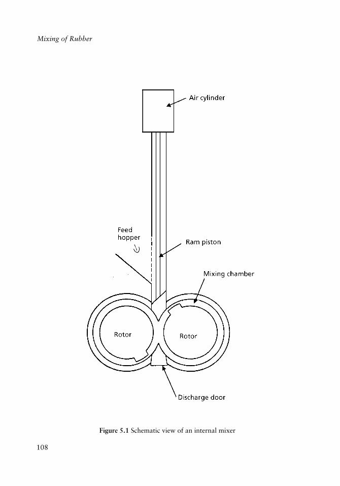
108

Mixing of Rubber

Figure 5.1 Schematic view of an internal mixer

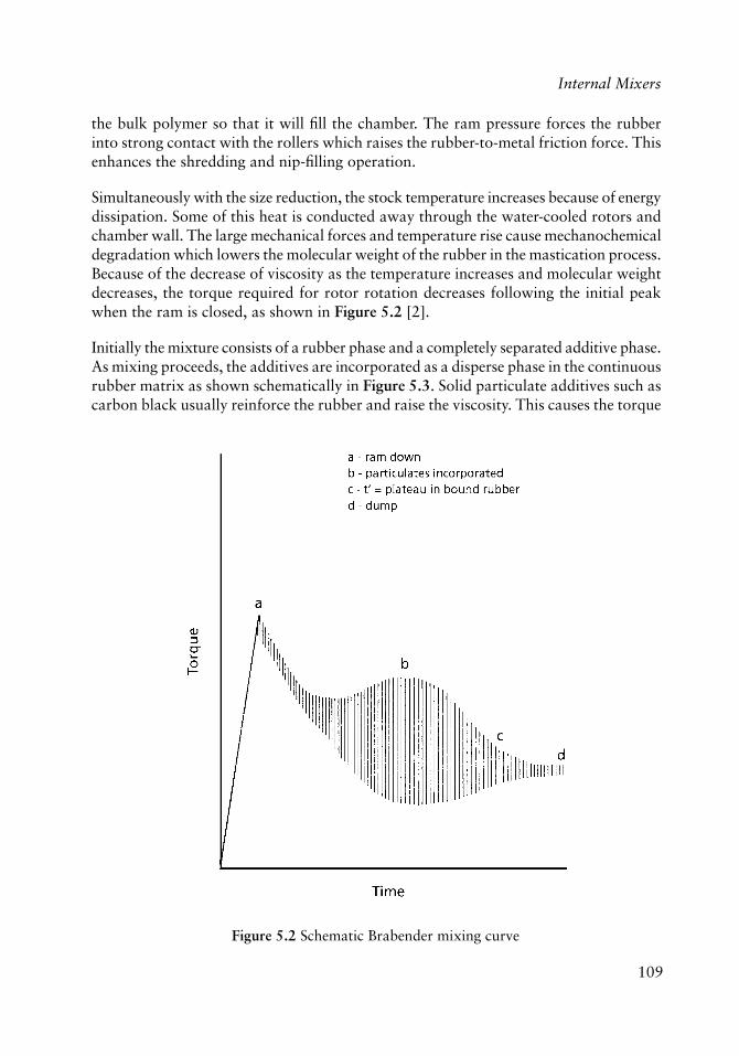
109

Internal Mixers

the bulk polymer so that it will fi ll the chamber. The ram pressure forces the rubber into strong contact with the rollers which raises the rubber-to-metal friction force. This enhances the shredding and nip-fi lling operation.

Simultaneously with the size reduction, the stock temperature increases because of energy dissipation. Some of this heat is conducted away through the water-cooled rotors and chamber wall. The large mechanical forces and temperature rise cause mechanochemical degradation which lowers the molecular weight of the rubber in the mastication process. Because of the decrease of viscosity as the temperature increases and molecular weight decreases, the torque required for rotor rotation decreases following the initial peak when the ram is closed, as shown in Figure 5.2 [2].

Initially the mixture consists of a rubber phase and a completely separated additive phase. As mixing proceeds, the additives are incorporated as a disperse phase in the continuous rubber matrix as shown schematically in Figure 5.3. Solid particulate additives such as carbon black usually reinforce the rubber and raise the viscosity. This causes the torque

Figure 5.2 Schematic Brabender mixing curve

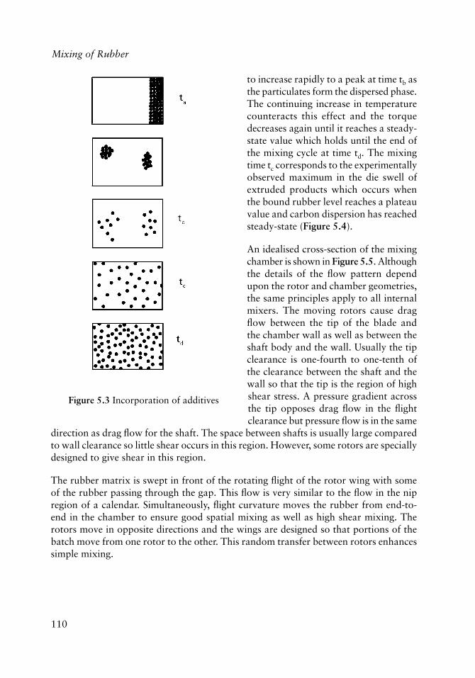
110

Mixing of Rubber

to increase rapidly to a peak at time tb as the particulates form the dispersed phase. The continuing increase in temperature counteracts this effect and the torque decreases again until it reaches a steady-state value which holds until the end of the mixing cycle at time td. The mixing time tc corresponds to the experimentally observed maximum in the die swell of extruded products which occurs when the bound rubber level reaches a plateau value and carbon dispersion has reached steady-state (Figure 5.4).

An idealised cross-section of the mixing chamber is shown in Figure 5.5. Although the details of the fl ow pattern depend upon the rotor and chamber geometries, the same principles apply to all internal mixers. The moving rotors cause drag fl ow between the tip of the blade and the chamber wall as well as between the shaft body and the wall. Usually the tip clearance is one-fourth to one-tenth of the clearance between the shaft and the wall so that the tip is the region of high shear stress. A pressure gradient across the tip opposes drag fl ow in the fl ight clearance but pressure fl ow is in the same

direction as drag fl ow for the shaft. The space between shafts is usually large compared to wall clearance so little shear occurs in this region. However, some rotors are specially designed to give shear in this region.

The rubber matrix is swept in front of the rotating fl ight of the rotor wing with some of the rubber passing through the gap. This fl ow is very similar to the fl ow in the nip region of a calendar. Simultaneously, fl ight curvature moves the rubber from end-to-end in the chamber to ensure good spatial mixing as well as high shear mixing. The rotors move in opposite directions and the wings are designed so that portions of the batch move from one rotor to the other. This random transfer between rotors enhances simple mixing.

Figure 5.3 Incorporation of additives

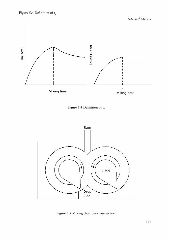
111

Internal Mixers

Figure 5.4 Defi nition of tc

Figure 5.5 Mixing chamber cross-section

Figure 5.4 Defi nition of tc

112

Mixing of Rubber

5.2 Analysis of an Internal Mixer

The fi rst analysis of an internal mixer was reported by Bolen and Colwell [3, 4] who used the simplifi ed geometry shown in Figure 5.6. The following symbols are used:

Ql = drag fl ow in channel

Q2 = drag fl ow at fl ight tip

Q3 = pressure fl ow in channel

Q4 = pressure fl ow at tip

g = tip clearance (constant)

h = channel clearance

e = tip width

s = length of rotor

N = rotor speed

Dc = diameter at shaft

Dt = diameter at tip

�c = viscosity of fl uid in channel

�t = viscosity of fl uid at tip

�P = pressure drop across fl ight

The viscosity at the tip need not equal the viscosity in the channel if the viscosity is shear dependent, even for isothermal fl ow. The directions of the four fl ow components are shown in Figure 5.6 when the barrel is considered to move relative to a stationary rotor. It is assumed that the radius of the rotor is large compared to the gap clearance so that the fl ow can be treated locally as fl ow between parallel plates in a Cartesian coordinate system. A constant viscosity is assumed in each region and the fl ow is treated locally. Then the solution for the drag fl ow components becomes:

Q1 = �DcshN/2 (5.1)

Q2 = �DtsgN/2 (5.2)

which is the total drag fl ow between parallel plates having a separation h (or g) and a relative velocity

V = �ND (5.3)

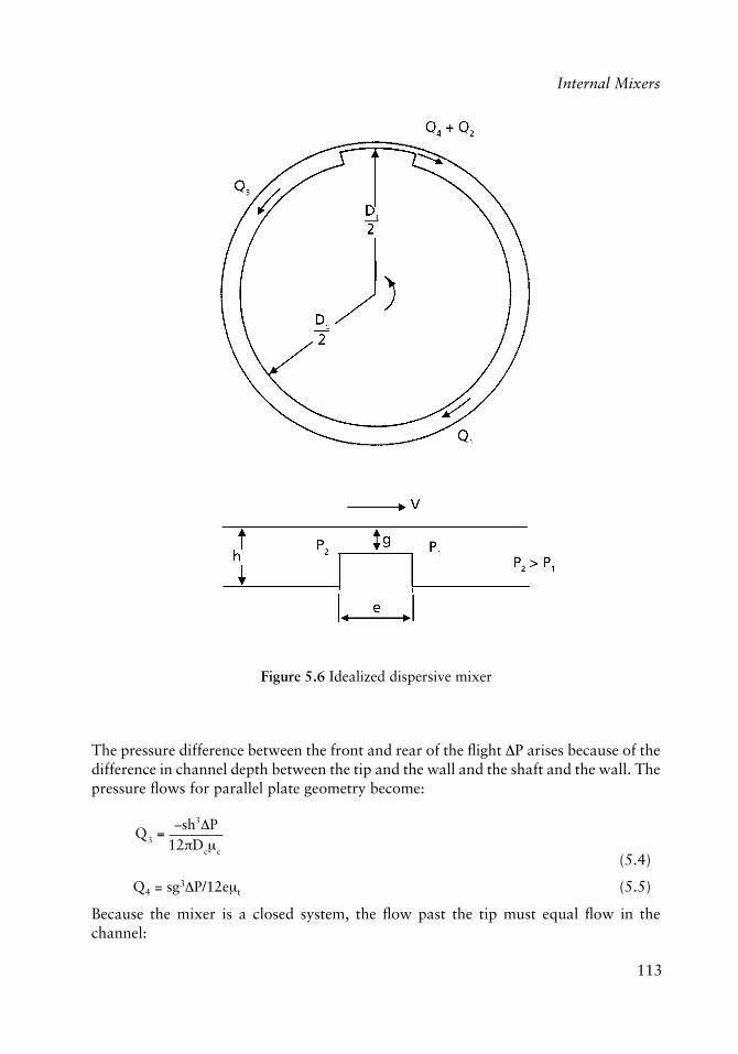
113

Internal Mixers

The pressure difference between the front and rear of the fl ight �P arises because of the difference in channel depth between the tip and the wall and the shaft and the wall. The pressure fl ows for parallel plate geometry become:

Q3 =

�sh3�P12�Dc�c

(5.4)

Q4 = sg3�P/12e�t (5.5)

Because the mixer is a closed system, the fl ow past the tip must equal fl ow in the channel:

Figure 5.6 Idealized dispersive mixer

114

Mixing of Rubber

Q1 + Q2 = Q3 + Q4 (5.6)

Substituting Equations (5.1)-(5.5) and solving for the pressure drop yields:

�P =6�N Dch�Dtg( )

h3

�Dc�c

+g3

e� t

�

��

�

��

(5.7)

Similar to the analysis used in the last chapter [Equation (4.85)), a velocity-average shear rate can be defi ned for both the tip and the channel:

�� =

u�� dy0

h

�

u dy0

h

� (5.8)

This is the same as a mass-averaged shear rate.

Let the ratio of pressure to drag fl ow be:

f = Qp/Qd (5.9)

fc = Q3/Q1 = f for channel (5.10a)

ft = Q4/Q2 = f for tip (5.10b)

Then the average shear rate is a function of f [3] and is given by:

�� =Q

sx2

0.75 1+ 3f( )4+ 72f2{ }

1+ 3f( )3

+ 1+ 9f( )

�

�

��

�

�

��

(5.11a)

if f > 1/3

�� =Q

sx2

21+ f( )

�

��

�

��

(5.11b)

if f > 1/3 < f < 1/3

�� =Q

sx2

1+ 3f( )4+144f2 1+ 3f( )4

72f2 1+ f( )

�

�

��

�

�

(5.11c)

if f > 1/3

where:

115

Internal Mixers

Q = Q1 and x2 = h2 in the channel, and

Q = Q2 and x2 = g2 in the tip.

The velocity profi le for combined fl ow between parallel plates [5] is given by:

vz =

vH

y y H y( )

2�dpdz

(5.12)

for plate separation H and relative velocity V. Then the shear rate may be calculated:

�� =

dvz

dy=

VH

1

2�dpdz

H 2y( ) (5.13)

The maximum shear stress will occur in the tip region where:

H = g (5.14a)

V = �DtN (5.14b)

dpdz

=�Pe

(5.14c)

The maximum shear rate and maximum shear stress for a Newtonian fl uid occur at y = g:

�max =��max

= �t

VH

+H2�

dpdz

�

�

�

�

=� t�DtN

g1+

3Dch

Dt

� g�

�

�

�

eh3

�g2Dc

+ g

�

�

�

��

(5.15)

The torque on the rotor is given by:

T =�

F.�

d�

�

SR

��

= �.�

A.�

d�

��

= s � t,y=0

eDt

z+ � y=0 Dc = e( ) Dc

z

�

��

�

�

(5.16)

Substituting into Equation (5.13) the appropriate values of V and H for the tip and for

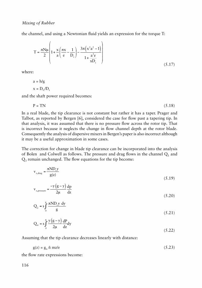
116

Mixing of Rubber

the channel, and using a Newtonian fl uid yields an expression for the torque T:

T =�N�

21+

xa

�xe�

1Dt

�

��

�

��

3� x2a2 �1( )1+

a3exDt

�

�

��

�

�

(5.17)

where:

a = h/g

x = DC/Dt

and the shaft power required becomes:

P = TN (5.18)

In a real blade, the tip clearance is not constant but rather it has a taper. Prager and Talbot, as reported by Bergen [6], considered the case for fl ow past a tapering tip. In that analysis, it was assumed that there is no pressure fl ow across the rotor tip. That is incorrect because it neglects the change in fl ow channel depth at the rotor blade. Consequently the analysis of dispersive mixers in Bergen’s paper is also incorrect although it may be a useful approximation in some cases.

The correction for change in blade tip clearance can be incorporated into the analysis of Bolen and Colwell as follows. The pressure and drag fl ows in the channel Q1 and Q3 remain unchanged. The fl ow equations for the tip become:

vz,drag =

�NDtyg(z)

(5.19)

vz,pressure =

y g y( )2�

dpdz

(5.20)

Q2 = s

�NDty dy

g0

g

� (5.21)

Q4 = s

y g � y( )2�

dPdz0

g

� dy

(5.22)

Assuming that the tip clearance decreases linearly with distance:

g(z) = go ñ mz/e (5.23)

the fl ow rate expressions become:

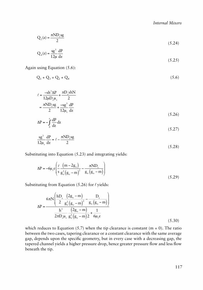
117

Internal Mixers

Q2(z) =

�NDtsg2

(5.24)

Q4(z) =

sg3

12�dPdz

(5.25)

Again using Equation (5.6):

Q1 + Q3 = Q2 + Q4 (5.6)

� =�sh3�P

12�Dc�c

+�DcshN

2

=�NDtsg

2+�sg3

12�t

dPdz

(5.26)

�P = �

dPdz

dz0

e

� (5.27)

sg3

12�t

dPdz

= � ��NDtsg

2 (5.28)

Substituting into Equation (5.23) and integrating yields:

�P = �6� te�

s

m �2go( )go

2 go �m( )2�

�NDt

go go �m( )

�

�

��

�

�

��

(5.29)

Substituting from Equation (5.26) for � yields:

�P =

6�NhDc

2

2go �m( )go

2 go �m( )2�

Dt

go go �m( )

�

�

��

�

�

��

h3

2�Dc�c

2go �m( )go

2 go �m( )2+

16�te

(5.30)

which reduces to Equation (5.7) when the tip clearance is constant (m = 0). The ratio between the two cases, tapering clearance or a constant clearance with the same average gap, depends upon the specifi c geometry, but in every case with a decreasing gap, the tapered channel yields a higher pressure drop, hence greater pressure fl ow and less fl ow beneath the tip.

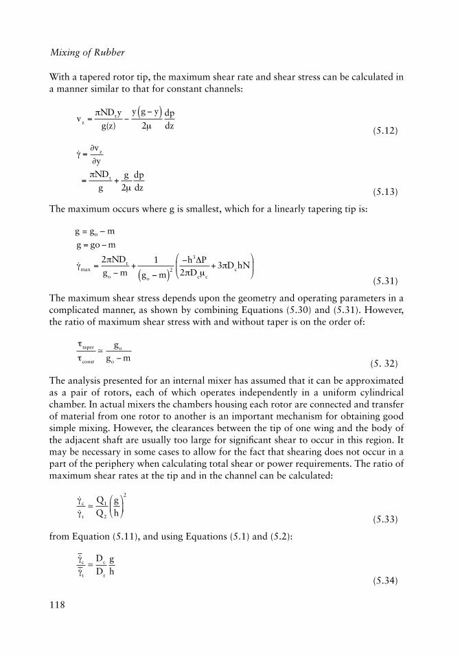
118

Mixing of Rubber

With a tapered rotor tip, the maximum shear rate and shear stress can be calculated in a manner similar to that for constant channels:

vz =

�NDty

g(z)�

y g � y( )2�

dpdz (5.12)

�� =�vz

�y

=�NDt

g+

g2�

dpdz (5.13)

The maximum occurs where g is smallest, which for a linearly tapering tip is:

g = go – m

g = go �m

��max =2�NDt

go �m+

1

go �m( )2

�h3�P2�Dc�c

+ 3�DchN�

�

�

�

(5.31)

The maximum shear stress depends upon the geometry and operating parameters in a complicated manner, as shown by combining Equations (5.30) and (5.31). However, the ratio of maximum shear stress with and without taper is on the order of:

� taper

�const

�go

go m (5. 32)

The analysis presented for an internal mixer has assumed that it can be approximated as a pair of rotors, each of which operates independently in a uniform cylindrical chamber. In actual mixers the chambers housing each rotor are connected and transfer of material from one rotor to another is an important mechanism for obtaining good simple mixing. However, the clearances between the tip of one wing and the body of the adjacent shaft are usually too large for signifi cant shear to occur in this region. It may be necessary in some cases to allow for the fact that shearing does not occur in a part of the periphery when calculating total shear or power requirements. The ratio of maximum shear rates at the tip and in the channel can be calculated:

��c

��t

�Q1

Q2

gh

�

��

�

��

2

(5.33)

from Equation (5.11), and using Equations (5.1) and (5.2):

��c

��t

�Dc

Dt

gh

(5.34)

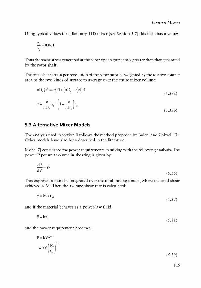
119

Internal Mixers

Using typical values for a Banbury 11D mixer (see Section 5.7) this ratio has a value:

��c

��t

� 0.061

Thus the shear stress generated at the rotor tip is signifi cantly greater than that generated by the rotor shaft.

The total shear strain per revolution of the rotor must be weighted by the relative contact area of the two kinds of surface to average over the entire mixer volume:

�Dc ��i1 = e��t i1+ �Dc � e( ) ��c i1

(5.35a)

�� =

e�Dc

��t + 1 =e

�Dc

�

��

�

� ��c

(5.35b)

5.3 Alternative Mixer Models

The analysis used in section B follows the method proposed by Bolen and Colwell [3]. Other models have also been described in the literature.

Mohr [7] considered the power requirements in mixing with the following analysis. The power P per unit volume in shearing is given by:

dPdV

= ��

(5.36)

This expression must be integrated over the total mixing time tm where the total shear achieved is M. Then the average shear rate is calculated:

�� = M / tM

(5.37)

and if the material behaves as a power-law fl uid:

� = k��n (5.38)

and the power requirement becomes:

P = kV��n+1

= kVMtm

�

��

�

��

n+1

(5.39)

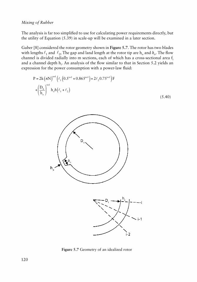
120

Mixing of Rubber

The analysis is far too simplifi ed to use for calculating power requirements directly, but the utility of Equation (5.39) in scale-up will be examined in a later section.

Guber [8] considered the rotor geometry shown in Figure 5.7. The rotor has two blades with lengths �1 and �2, The gap and land length at the rotor tip are ho and �o. The fl ow channel is divided radially into m sections, each of which has a cross-sectional area fi and a channel depth hi. An analysis of the fl ow similar to that in Section 5.2 yields an expression for the power consumption with a power-law fl uid:

P = 2k �N( )n+1�1 0.5n+1 + 0.865n+1( ) + 2�20.75n+1( ) F

+Dk

ho

�

��

�

�

n+1

ho� �1 + �2( ) (5.40)

Figure 5.7 Geometry of an idealized rotor

121

Internal Mixers

where:

F =

Dk

hi

� 2�

��

�

�

n+1

fii=1

m

� (5.41)

and Dk is the outer chamber diameter. Equation (5.40) has the form:

P = f(geometry) k Nn+lU3� (5.42)

where U is a scaling length and � corresponds to a fi lling parameter. For two geometrically similar mixers, the scaling-law for power requirements becomes:

P1

P2

=k1

k2

N1

N2

�

��

�

��

n+1

U3�

(5.43)

where:

u =

D1

D2

=�11

�12

=�21

�22

=ho1

ho2

=�1

�2

and

� = F1/F2

This is the same result as predicted from Mohr’s analysis where:

N�1 / tm (5.44a)

V�U3

(5.44b)

and is similar to the equivalent expression derived in Section 5.2 for power-law fl uid [Equation (5.17)].

Starov and co-workers [9] compared the power requirements to achieve the same dispersion on a single machine for a synthetic. rubber as a function of ram pressure and rotor speed. This is equivalent to allowing the mixing time to vary at constant total work with a variable shaft power (see Section 5.7). They found the empirical expressions:

P = A + B Pr (5 .45a)

P = C + Dn (5.45b)

where P is the power in kW and Pr and n are the ram pressure and rotor speed. The data is summarised in Table 5.1. This correlation is not generally useful because it does not include geometry and material variables. For many rubbers, the power-law exponent is

122

Mixing of Rubber

approximately 0.2 - 0.3 in which case the seemingly linear response over a limited range of operating variables for a constant geometry and material is a reasonable approximation to the more general analysis presented earlier. The operating curves for a single machine often have a simple expression such as Equation (5.45). However, these are usually approximations to more complex equations such as Equations (5.17)-(5.18) or (5.39), and the simple operating lines would give incorrect predictions if used for scale-up.

Stupachenko, Bebris and Pukhov [10, 11] considered an heuristic model for the mixing process. In their model, they assumed all materials were loaded simultaneously; the shear gradient was constant; material properties were constant; machine temperature was constant; and the rate of particle incorporation was rapid compared to the rate of mixing.

Let:

Qp = rate of mix production

�* = mix viscosity

P = power

Vp

*� = proportion of volume as powder in mix

Vp� = proportion of volume as powder not in mix

Vp� (0) = initial powder volume fraction p

� = time

Then the rate of mix production is given by:

Table 5.1 Power requirements (Pr) for mixingn (rpm) Pr range (kg/cm2) A (kW) B32 0.88-1.32 4.05 0.5750 0.66-1.32 5.26 1.4180 0.88-1.32 7.76 2.41100 0.66-1.32 9.70 2.36

Pr (kg/cm2) N range (rpm) C (kW) D (kW/rpm)0.66 32-100 1.25 0.10.88 32.100 1.8 0.11.32 32.100 1.25 0.12

123

Internal Mixers

�p =

dd�

Vp* = k �*( )k P( ) Vp��

(5.46)

and

Vp� = Vp� 0( ) � �pd��

0

�

� (5.47)

which states that the rate of mix production is proportional to the amount of undispersed powder, and that the rate is a function of the shaft power (i.e., shear rate) and the material viscosity. The rate constants are assumed to have the form:

k(�*) = Be-c�* (5.48a)

and

k(P) = k*P (5. 48b)

where B, c and k* are constants.

The time dependence of the material response is given by a two-dimensional linear viscoelastic model:

d2�

d�2+

E1

�1

+E1

�2

+E2

�2

�

��

�

��d�d�

+E1E2�

�1�2

=E1E2

�2

d�d�

(5.49)

where:

E1 = initial elastic modulus

E2 = elastic modulus

�1 = steady shear viscosity

�2 = viscosity of elastic after-effect (creep recovery)

T = temperature

�- = initial mix viscosity

= �(0) �(T) � (.V*p) (5.50)

This expression becomes a power-law model following an initial transient. The viscosity components are given by:

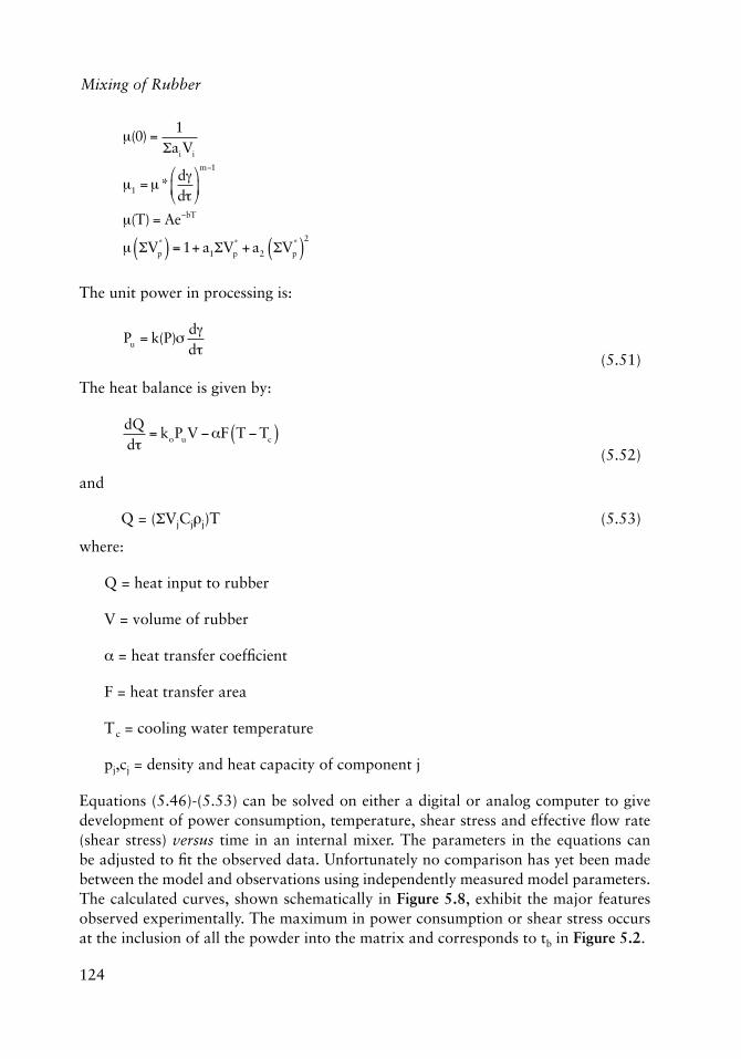
124

Mixing of Rubber

�(0) =1

�aiVi

�1 =�*d�d�

�

��

�

m1

�(T) = AebT

� �Vp*( ) = 1+ a1�Vp

* + a2 �Vp*( )

2

The unit power in processing is:

Pu = k(P)�

d�d�

(5.51)

The heat balance is given by:

dQd�

= koPuV �F T Tc( ) (5.52)

and

Q = (.VjCj,j)T (5.53)

where:

Q = heat input to rubber

V = volume of rubber

� = heat transfer coeffi cient

F = heat transfer area

Tc = cooling water temperature

pj,cj = density and heat capacity of component j

Equations (5.46)-(5.53) can be solved on either a digital or analog computer to give development of power consumption, temperature, shear stress and effective fl ow rate (shear stress) versus time in an internal mixer. The parameters in the equations can be adjusted to fi t the observed data. Unfortunately no comparison has yet been made between the model and observations using independently measured model parameters. The calculated curves, shown schematically in Figure 5.8, exhibit the major features observed experimentally. The maximum in power consumption or shear stress occurs at the inclusion of all the powder into the matrix and corresponds to tb in Figure 5.2.

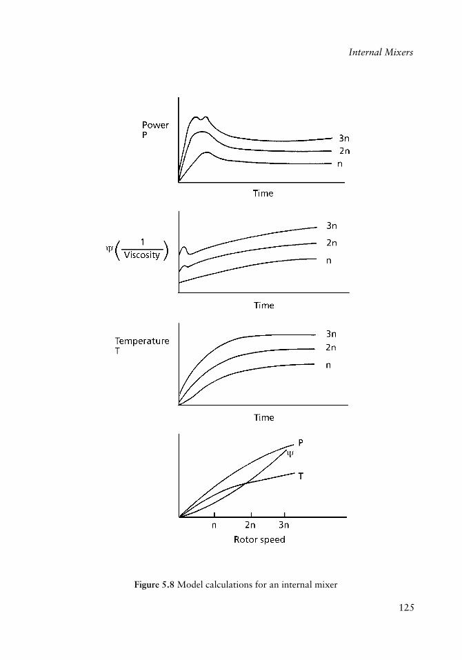
125

Internal Mixers

Figure 5.8 Model calculations for an internal mixer

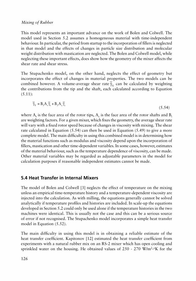
126

Mixing of Rubber

This model represents an important advance on the work of Bolen and Colwell. The model used in Section 5.2 assumes a homogeneous material with time-independent behaviour. In particular, the period from startup to the incorporation of fi llers is neglected in that model and the effects of changes in particle size distribution and molecular weight distribution with mastication are neglected. The Bolen and Colwell model, while neglecting these important effects, does show how the geometry of the mixer affects the shear rate and shear stress.

The Stupachenko model, on the other hand, neglects the effect of geometry but incorporates the effect of changes in material properties. The two models can be combined however. A volume-average shear rate ��V

can be calculated by weighting the contributions from the tip and the shaft, each calculated according to Equation (5.11):

��V = B1At ��t + B2Ac ��c

(5.54)

where At is the face area of the rotor tips, Ac is the face area of the rotor shafts and Bi are weighting factors. For a given mixer, which fi xes the geometry, the average shear rate will vary with a fi xed rotor speed because of changes in viscosity with mixing. The shear rate calculated in Equation (5.54) can then be used in Equation (5.49) to give a more complete model. The main diffi culty in using this combined model is in determining how the material functions such as modulus and viscosity depend upon the incorporation of fi llers, mastication and other time-dependent variables. In some cases, however, estimates of the material behaviour, such as the temperature dependence of viscosity, can be made. Other material variables may be regarded as adjustable parameters in the model for calculation purposes if reasonable independent estimates cannot be made.

5.4 Heat Transfer in Internal Mixers

The model of Bolen and Colwell [3] neglects the effect of temperature on the mixing unless an empirical time-temperature history and a temperature-dependent viscosity are injected into the calculation. As with milling, the equations generally cannot be solved analytically if temperature profi les and histories are included. In scale-up the equations developed in Section 5.2 could only be used alone if the temperature histories in the two machines were identical. This is usually not the case and this can be a serious source of error if not recognised. The Stupachenko model incorporates a simple heat transfer model in Equation (5.52).

The main diffi culty in using this model is in obtaining a reliable estimate of the heat transfer coeffi cient. Kapitonov [12] estimated the heat transfer coeffi cient from experiments with a natural rubber mix on an RS-2 mixer which has open cooling and sprinkled water on the housing. He obtained values of 250 - 270 W/m2-oK for the

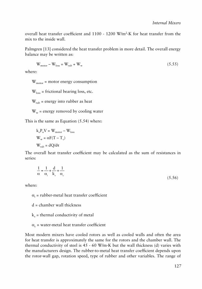
127

Internal Mixers

overall heat transfer coeffi cient and 1100 - 1200 W/m2-K for heat transfer from the mix to the inside wall.

Palmgren [13] considered the heat transfer problem in more detail. The overall energy balance may be written as:

Wmotor – Wloss = Wrub + Ww (5.55)

where:

Wmotor = motor energy consumption

Wloss = frictional bearing loss, etc.

Wrub = energy into rubber as heat

Ww = energy removed by cooling water

This is the same as Equation (5.54) where:

koPuV = Wmotor – Wloss

Ww = �F(T – Tc)

Wrub = dQ/d�

The overall heat transfer coeffi cient may be calculated as the sum of resistances in series:

1�

=1�i

+dks

+1�c

(5.56)

where:

�i = rubber-metal heat transfer coeffi cient

d = chamber wall thickness

ks = thermal conductivity of metal

�c = water-metal heat transfer coeffi cient

Most modern mixers have cooled rotors as well as cooled walls and often the area for heat transfer is approximately the same for the rotors and the chamber wall. The thermal conductivity of steel is 45 - 60 W/m-K but the wall thickness (d) varies with the manufacturers design. The rubber-to-metal heat transfer coeffi cient depends upon the rotor-wall gap, rotation speed, type of rubber and other variables. The range of

128

Mixing of Rubber

reported values is 1100 - 6000 W/m2-K but 1100 - 1500 W/m2-K seems a more reliable estimate. The cooling water-side coeffi cient �c depends upon the rate of water fl ow, the channel design and fouling of the channel walls. Typical values are 2000 - 10,000 W/m2-K. Substituting these values into Equation (5.56) shows that resistance to heat transfer through the metal wall and to the cooling water make signifi cant contributions to the overall heat transfer coeffi cients.

An estimate of the heat transfer coeffi cient can be made by considering the model proposed by Jepson [14] which treats heat transfer at the wall as a scraped-surface heat exchanger. As the rotor tip in Figure 5.6 passes any point on the circumference, a new layer of material is laid down on that point. The temperature of the layer at the time of fi rst contact, t = 0, is the bulk temperature of the rubber in the mixer. The surface of the layer immediately assumes the mixer wall temperature with which it is in contact. Heat is transferred from the bulk of the rubber layer to its surface by conduction during the contact time which is the time interval between successive passes of the blade at that point when one layer replaces the previous layer.

Let the total heat loss during one revolution of the blade be:

qT = �cph T

� Tb( )

(5.57)

where:

,,cp = density, heat capacity

T� = average temperature in layer

Tb = bulk rubber temperature

h = channel depth

qT = heat loss per unit wall area

During the period of one revolution, the heat transfer to the wall is:

qT = �i(Tw ñ Tb)/N (5.58)

where:

�i = rubber-metal heat transfer coeffi cient

Tw = metal-wall temperature

N = rate of rotor rotation

129

Internal Mixers

The average temperature in the rubber layer can be calculated from the unsteady-state heat conduction expression:

�T�t

=k�cp

�2T�y2

(5.59)

with boundary conditions:

t < 0, T(y) = Tb

t > 0, T(O) = Tw

T(h) = Tw

and the average layer temperature:

T� =

1h

T y( )dy0

h

� (5.60)

where:

k = thermal conductivity of rubber

y = distance into the layer

Combining Equations (5.57)-(5.60) yields:

F s2( ) =Tw �T

�

Tw �Tb

=8�2

e�s2

+19

e�9s2

+…�

��

�

� (5.61)

where:

s2 =�2

4ktc

�cph

tc = 2�/Nn

n = number of blade tips

and

�i = �cphN(l ñ F(s2)) (5.62)

The effect of the fl ight clearance is accounted for by considering that there is a stagnant fi lm between the renewed layer and the wall. In this case:

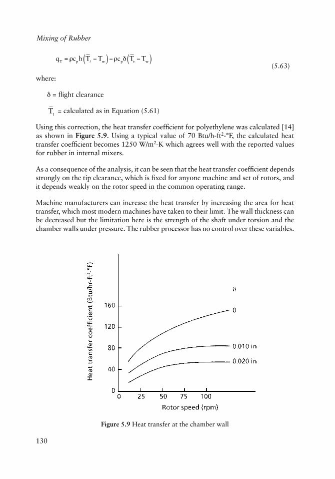
130

Mixing of Rubber

qT = �cph T

� Tw( ) �cp� Tt Tw( )

(5.63)

where:

� = fl ight clearance

Tt = calculated as in Equation (5.61)

Using this correction, the heat transfer coeffi cient for polyethylene was calculated [14] as shown in Figure 5.9. Using a typical value of 70 Btu/h-ft2-°F, the calculated heat transfer coeffi cient becomes 1250 W/m2-K which agrees well with the reported values for rubber in internal mixers.

As a consequence of the analysis, it can be seen that the heat transfer coeffi cient depends strongly on the tip clearance, which is fi xed for anyone machine and set of rotors, and it depends weakly on the rotor speed in the common operating range.

Machine manufacturers can increase the heat transfer by increasing the area for heat transfer, which most modern machines have taken to their limit. The wall thickness can be decreased but the limitation here is the strength of the shaft under torsion and the chamber walls under pressure. The rubber processor has no control over these variables.

Figure 5.9 Heat transfer at the chamber wall

131

Internal Mixers

The heat transfer coeffi cient on the water side can be increased by raising the water fl ow rate and the overall heat transfer can be increased by using chilled water which increases the temperature difference. One major factor in the water-side heat transfer coeffi cient is fouling of the walls. Particularly in older machines this is the single most important resistance to heat transfer and it can be a major cause for decreased performance as a machine ages.

The temperature of the rubber depends upon a balance between the rate of heat generation and the rate of heat removal. Often there is a maximum temperature limit for the material to prevent degradation or gelling or scorchiness in the product. This maximum allowable temperature criterion usually limits the maximum allowable rate of mixing in a rapid internal mixing.

5.5 The Effect of Ram Pressure

Until the late 1950s the standard internal mixer was operated with a ram pressure little over one atmosphere, often around 16 psi. At this pressure it was found that a large proportion of the mixing cycle was used to shred and masticate the rubber suffi ciently for the matrix to fi ll the fl ow channel. The rotors tended to slip past the stock and the ram oscillated up and down with the frequency of the rotors as the rubber entered and retracted from the nip between the rotors. Gradually the temperature increased suffi ciently for fl ow in the gaps to begin and effi cient mixing commenced. This is exactly the behaviour, observed in region 1 and the region 1 2 transition as described in Chapter 4 for milling instability.

The fl ow in region 1 where the stock oscillates in the nip is controlled by a critical stress at the rotor wall where slip occurs. The effect of increasing pressure is to increase the contact force between the rubber and the rotor surface. This has the effect of increasing the critical stress so that fl ow begins at a lower temperature. This means that effective milling begins much earlier in the cycle and because the stock temperature is lower at this point, the viscosity is higher and the power peak is higher. The higher viscosity means that particle dispersion is improved because shear stresses are higher. The rotor speed can be increased before slip occurs so that the mixing time for a constant total shear can be decreased.

The combined effects of these processes are shown in Figures 5.10 and 5.11. A typical set of power profi les for two ram pressures in the same RS-2 mixer with the same rubber recipe are shown in Figure 5.10 from the data of Bebris and co-workers [15]. When the ram pressure was doubled, the average power increased from 92 to 170 kW, but because the mixing time could be reduced from 13 to 6 minutes the total energy consumption remained essentially constant. The rotor speed was doubled for the high pressure process to 20 rpm versus 9 rpm for the low pressure process.

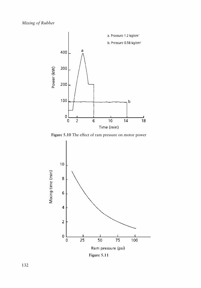
132

Mixing of Rubber

Figure 5.10 The effect of ram pressure on motor power

Figure 5.11

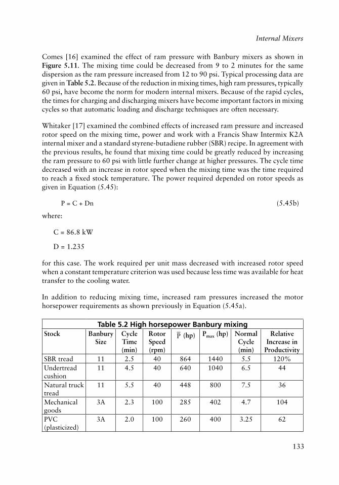
133

Internal Mixers

Comes [16] examined the effect of ram pressure with Banbury mixers as shown in Figure 5.11. The mixing time could be decreased from 9 to 2 minutes for the same dispersion as the ram pressure increased from 12 to 90 psi. Typical processing data are given in Table 5.2. Because of the reduction in mixing times, high ram pressures, typically 60 psi, have become the norm for modern internal mixers. Because of the rapid cycles, the times for charging and discharging mixers have become important factors in mixing cycles so that automatic loading and discharge techniques are often necessary.

Whitaker [17] examined the combined effects of increased ram pressure and increased rotor speed on the mixing time, power and work with a Francis Shaw Intermix K2A internal mixer and a standard styrene-butadiene rubber (SBR) recipe. In agreement with the previous results, he found that mixing time could be greatly reduced by increasing the ram pressure to 60 psi with little further change at higher pressures. The cycle time decreased with an increase in rotor speed when the mixing time was the time required to reach a fi xed stock temperature. The power required depended on rotor speeds as given in Equation (5.45):

P = C + Dn (5.45b)

where:

C = 86.8 kW

D = 1.235

for this case. The work required per unit mass decreased with increased rotor speed when a constant temperature criterion was used because less time was available for heat transfer to the cooling water.

In addition to reducing mixing time, increased ram pressures increased the motor horsepower requirements as shown previously in Equation (5.45a).

Table 5.2 High horsepower Banbury mixingStock Banbury

SizeCycle Time (min)

Rotor Speed (rpm)

P (hp) Pmax (hp) Normal Cycle (min)

Relative Increase in

ProductivitySBR tread 11 2.5 40 864 1440 5.5 120%Undertread cushion

11 4.5 40 640 1040 6.5 44

Natural truck tread

11 5.5 40 448 800 7.5 36

Mechanical goods

3A 2.3 100 285 402 4.7 104

PVC (plasticized)

3A 2.0 100 260 400 3.25 62

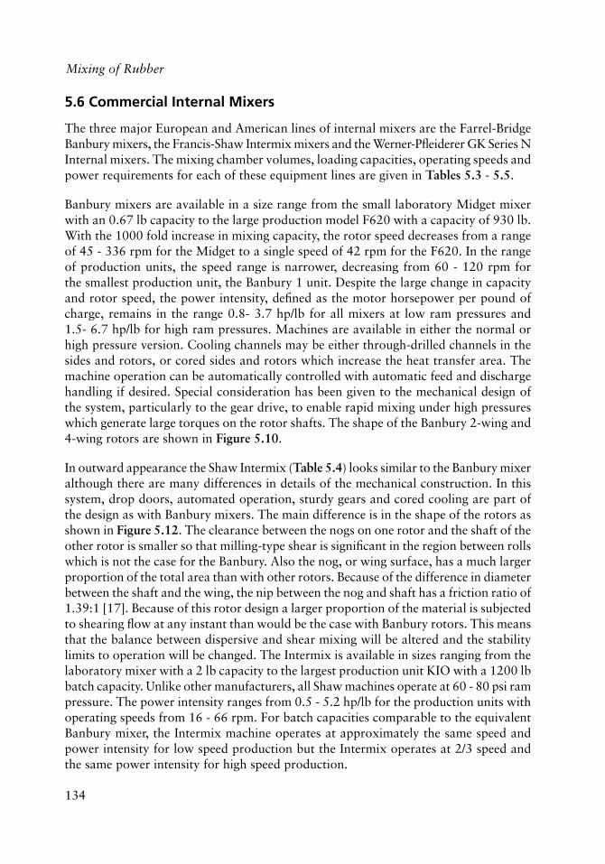
134

Mixing of Rubber

5.6 Commercial Internal Mixers

The three major European and American lines of internal mixers are the Farrel-Bridge Banbury mixers, the Francis-Shaw Intermix mixers and the Werner-Pfl eiderer GK Series N Internal mixers. The mixing chamber volumes, loading capacities, operating speeds and power requirements for each of these equipment lines are given in Tables 5.3 - 5.5.

Banbury mixers are available in a size range from the small laboratory Midget mixer with an 0.67 lb capacity to the large production model F620 with a capacity of 930 lb. With the 1000 fold increase in mixing capacity, the rotor speed decreases from a range of 45 - 336 rpm for the Midget to a single speed of 42 rpm for the F620. In the range of production units, the speed range is narrower, decreasing from 60 - 120 rpm for the smallest production unit, the Banbury 1 unit. Despite the large change in capacity and rotor speed, the power intensity, defi ned as the motor horsepower per pound of charge, remains in the range 0.8- 3.7 hp/lb for all mixers at low ram pressures and 1.5- 6.7 hp/lb for high ram pressures. Machines are available in either the normal or high pressure version. Cooling channels may be either through-drilled channels in the sides and rotors, or cored sides and rotors which increase the heat transfer area. The machine operation can be automatically controlled with automatic feed and discharge handling if desired. Special consideration has been given to the mechanical design of the system, particularly to the gear drive, to enable rapid mixing under high pressures which generate large torques on the rotor shafts. The shape of the Banbury 2-wing and 4-wing rotors are shown in Figure 5.10.

In outward appearance the Shaw Intermix (Table 5.4) looks similar to the Banbury mixer although there are many differences in details of the mechanical construction. In this system, drop doors, automated operation, sturdy gears and cored cooling are part of the design as with Banbury mixers. The main difference is in the shape of the rotors as shown in Figure 5.12. The clearance between the nogs on one rotor and the shaft of the other rotor is smaller so that milling-type shear is signifi cant in the region between rolls which is not the case for the Banbury. Also the nog, or wing surface, has a much larger proportion of the total area than with other rotors. Because of the difference in diameter between the shaft and the wing, the nip between the nog and shaft has a friction ratio of 1.39:1 [17]. Because of this rotor design a larger proportion of the material is subjected to shearing fl ow at any instant than would be the case with Banbury rotors. This means that the balance between dispersive and shear mixing will be altered and the stability limits to operation will be changed. The Intermix is available in sizes ranging from the laboratory mixer with a 2 lb capacity to the largest production unit KIO with a 1200 lb batch capacity. Unlike other manufacturers, all Shaw machines operate at 60 - 80 psi ram pressure. The power intensity ranges from 0.5 - 5.2 hp/lb for the production units with operating speeds from 16 - 66 rpm. For batch capacities comparable to the equivalent Banbury mixer, the Intermix machine operates at approximately the same speed and power intensity for low speed production but the Intermix operates at 2/3 speed and the same power intensity for high speed production.

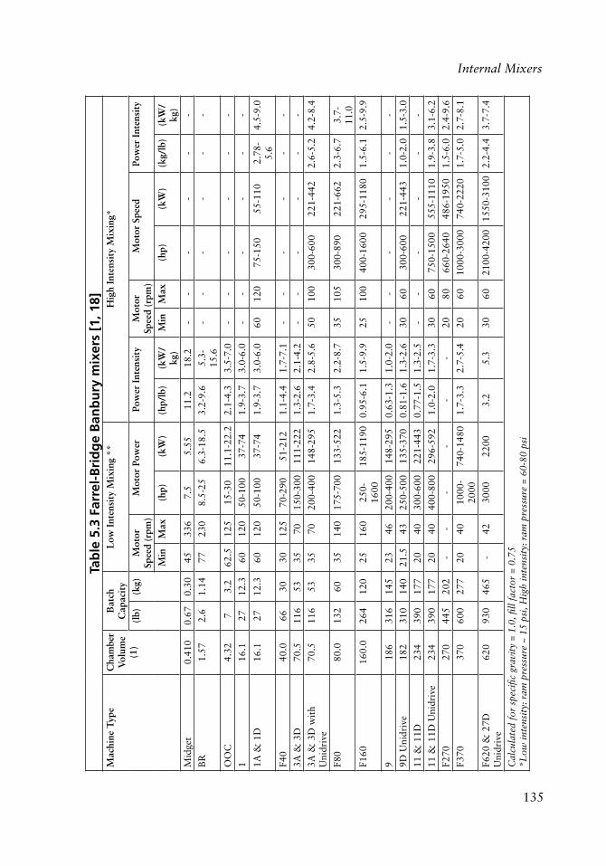
135

Internal Mixers

Tab

le 5

.3 F

arre

l-B

rid

ge

Ban

bu

ry m

ixer

s [1

, 18]

Mac

hine

Typ

eC

ham

ber

Vol

ume

(1)

Bat

ch

Cap

acit

yL

ow I

nten

sity

Mix

ing

**H

igh

Inte

nsit

y M

ixin

g*

(lb)

(kg)

Mot

or

Spee

d (r

pm)

Mot

or P

ower

Pow

er I

nten

sity

Mot

or

Spee

d (r

pm)

Mot

or S

peed

Pow

er I

nten

sity

Min

Max

(hp)

(kW

)(h

p/lb

)(k

W/

kg)

Min

Max

(hp)

(kW

)(k

g/lb

)(k

W/

kg)

Mid

get

0.41

00.

670.

3045

336

7.5

5.55

11.2

18.2

--

--

--

BR

1.57

2.6

1.14

7723

08.

5-25

6.3-

18.5

3.2-

9.6

5.3-

15.6

--

--

--

OO

C4.

327

3.2

62.5

125

15-3

011

.1-2

2.2

2.1-

4.3

3.5-

7.0

--

--

--

116

.127

12.3

6012

050

-100

37-7

41.

9-3.

73.

0-6.

0-

--

--

-

1A &

1D

16.1

2712

.360

120

50-1

0037

-74

1.9-

3.7

3.0-

6.0

6012

075

-150

55-1

102.

78-

5.6

4.5-

9.0

F40

40.0

6630

3012

570

-290

51-2

121.

1-4.

41.

7-7.

1-

--

--

-

3A &

3D

70.5

116

5335

7015

0-30

011

1-22

21.

3-2.

62.

1-4.

2-

--

--

-

3A &

3D

wit

h U

nidr

ive

70.5

116

5335

7020

0-40

014

8-29

51.

7-3.

42.

8-5.

650

100

300-

600

221-

442

2.6-

5.2

4.2-

8.4

F80

80.0

132

6035

140

175-

700

133-

522

1.3-

5.3

2.2-

8.7

3510

530

0-89

022

1-66

22.

3-6.

73.

7-11

.0

F160

160.

026

412

025

160

250-

1600

185-

1190

0.95

-6.1

1.5-

9.9

2510

040

0-16

0029

5-11

801.

5-6.

12.

5-9.

9

918

631

614

523

4620

0-40

014

8-29

50.

63-1

.31.

0-2.

0-

--

--

-

9D U

nidr

ive

182

310

140

21.5

4325

0-50

013

5-37

00.

81-1

.61.

3-2.

630

6030

0-60

022

1-44

31.

0-2.

01.

5-3.

0

11 &

11D

234

390

177

2040

300-

600

221-

443

0.77

-1.5

1.3-

2.5

--

--

--

11 &

11D

Uni

driv

e23

439

017

720

4040

0-80

029

6-59

21.

0-2.

01.

7-3.

330

6075

0-15

0055

5-11

101.

9-3.

83.

1-6.

2

F270

270

445

202

--

--

--

2080

660-

2640

486-

1950

1.5-

6.0

2.4-

9.6

F370

370

600

277

2040

1000

-20

0074

0-14

801.

7-3.

32.

7-5.

420

6010

00-3

000

740-

2220

1.7-

5.0

2.7-

8.1

F620

& 2

7D

Uni

driv

e62

093

046

5-

4230

0022

003.

25.

330

6021

00-4

200

1550

-310

02.

2-4.

43.

7-7.

4

Cal

cula

ted

for

spec

ifi c

grav

ity

= 1.

0, fi

ll fa

ctor

= 0

.75

*Low

inte

nsit

y: r

am p

ress

ure

~ 15

psi

, Hig

h in

tens

ity:

ram

pre

ssur

e =

60-8

0 ps

i

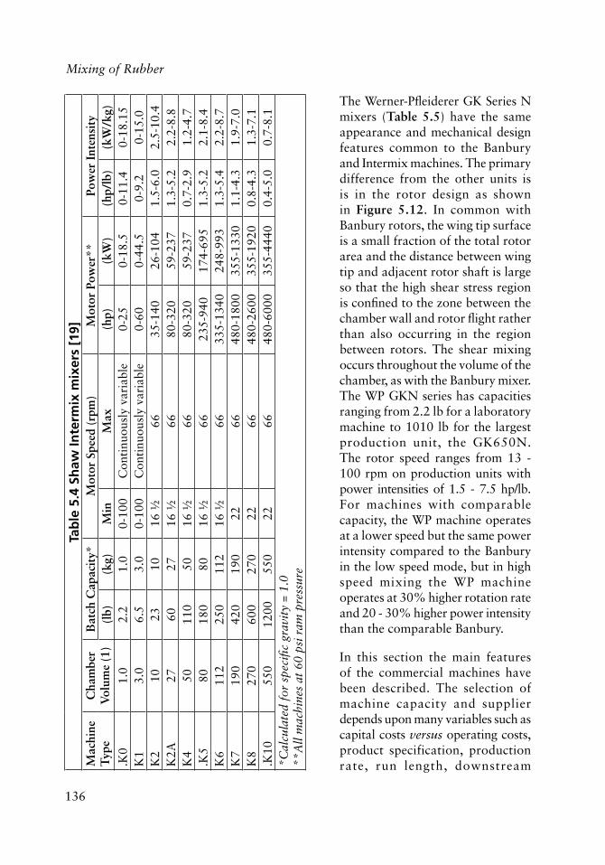
136

Mixing of Rubber

The Werner-Pfl eiderer GK Series N mixers (Table 5.5) have the same appearance and mechanical design features common to the Banbury and Intermix machines. The primary difference from the other units is is in the rotor design as shown in Figure 5.12. In common with Banbury rotors, the wing tip surface is a small fraction of the total rotor area and the distance between wing tip and adjacent rotor shaft is large so that the high shear stress region is confi ned to the zone between the chamber wall and rotor fl ight rather than also occurring in the region between rotors. The shear mixing occurs throughout the volume of the chamber, as with the Banbury mixer. The WP GKN series has capacities ranging from 2.2 lb for a laboratory machine to 1010 lb for the largest production unit, the GK650N. The rotor speed ranges from 13 - 100 rpm on production units with power intensities of 1.5 - 7.5 hp/lb. For machines with comparable capacity, the WP machine operates at a lower speed but the same power intensity compared to the Banbury in the low speed mode, but in high speed mixing the WP machine operates at 30% higher rotation rate and 20 - 30% higher power intensity than the comparable Banbury.

In this section the main features of the commercial machines have been described. The selection of machine capacity and supplier depends upon many variables such as capital costs versus operating costs, product specification, production rate, run length, downstream

Tab

le 5

.4 S

haw

Inte

rmix

mix

ers

[19]

Mac

hine

T

ype

Cha

mbe

r V

olum

e (1

)B

atch

Cap

acit

y*M

otor

Spe

ed (

rpm

)M

otor

Pow

er**

Pow

er I

nten

sity

(lb)

(kg)

Min

Max

(hp)

(kW

)(h

p/lb

)(k

W/k

g).K

01.

02.

21.

00-

100

Con

tinu

ousl

y va

riab

le0-

250-

18.5

0-11

.40-

18.1

5K

13.

06.

53.

00-

100

Con

tinu

ousl

y va

riab

le0-

600-

44.5

0-9.

20-

15.0

K2

1023

1016

½66

35-1

4026

-104

1.5-

6.0

2.5-

10.4

K2A

2760

2716

½66

80-3

2059

-237

1.3-

5.2

2.2-

8.8

K4

5011

050

16 ½

6680

-320

59-2

370.

7-2.

91.

2-4.

7.K

580

180

8016

½66

235-

940

174-

695

1.3-

5.2

2.1-

8.4

K6

112

250

112

16 ½

6633

5-13

4024

8-99

31.

3-5.

42.

2-8.

7K

719

042

019

022

6648

0-18

0035

5-13

301.

1-4.

31.

9-7.

0K

827

060

027

022

6648

0-26

0035

5-19

200.

8-4.

31.

3-7.

1.K

1055

012

0055

022

6648

0-60

0035

5-44

400.

4-5.

00.

7-8.

1*C

alcu

late

d fo

r sp

ecifi

c gr

avit

y =

1.0

**A

ll m

achi

nes

at 6

0 ps

i ram

pre

ssur

e

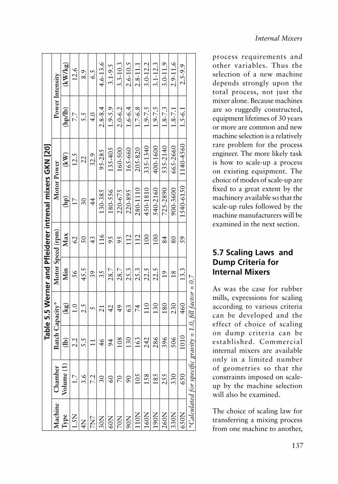
137

Internal MixersTa

ble

5.5

Wer

ner

an

d P

fl ei

der

er in

tren

al m

ixer

s G

KN

[20

]M

achi

ne

Typ

eC

ham

ber

Vol

ume

(1)

Bat

ch C

apac

ity*

Mot

or S

peed

(rp

m)

Mot

or P

ower

Pow

er I

nten

sity

(lb)

(kg)

Min

Max

(hp)

(kW

)(h

p/lb

)(k

W/k

g)1.

5N1.

72.

21.

056

6217

12.5

7.7

12.6

4N3.

65.

52.

545

.550

3022

5.5

8.9

7N7

7.2

115

3943

4432

.94.

06.

530

N30

4621

3511

613

0-38

595

-285

2.8-

8.4

4.6-

13.6

60N

6094

4228

.795

180-

556

135-

405

1.9-

5.9

3.1-

9.5

70N

7010

849

28.7

9522

0-67

516

0-50

02.

0-6.

23.

3-10

.390

N90

130

6325

.311

222

0-89

516

5-66

01.

6-6.

42.

6-10

.511

0N10

516

374

25.3

112

280-

1110

205-

820

1.7-

6.8

2.8-

11.1

160N

158

242

110

22.5

100

450-

1810

335-

1340

1.9-

7.5

3.0-

12.2

190N

185

286

130

22.5

100

540-

2160

400-

1600

1.9-

7.5

3.1-

12.3

260N

255

396

180

1984

725-

2890

535-

2140

1.8-

7.3

3.0-

11.9

330N

330

506

230

1880

900-

3600

665-

2660

1.8-

7.1

2.9-

11.6

650N

650

1010

460

13.3

5915

40-6

150

1140

-456

01.

5-6.

12.

5-9.

9*C

alcu

late

d fo

r sp

ecifi

c gr

avit

y =

1.0,

fi ll

fact

or =

0.7

process requirements and other variables. Thus the selection of a new machine depends strongly upon the total process, not just the mixer alone. Because machines are so ruggedly constructed, equipment lifetimes of 30 years or more are common and new machine selection is a relatively rare problem for the process engineer. The more likely task is how to scale-up a process on existing equipment. The choice of modes of scale-up are fi xed to a great extent by the machinery available so that the scale-up rules followed by the machine manufacturers will be examined in the next section.

5.7 Scaling Laws and Dump Criteria for Internal Mixers

As was the case for rubber mills, expressions for scaling according to various criteria can be developed and the effect of choice of scaling on dump criteria can be established. Commercial internal mixers are available only in a limited number of geometries so that the constraints imposed on scale-up by the machine selection will also be examined.

The choice of scaling law for transferring a mixing process from one machine to another,

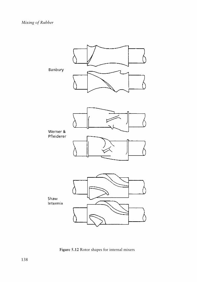
138

Mixing of Rubber

Figure 5.12 Rotor shapes for internal mixers

139

Internal Mixers

such as a laboratory mixer to a production unit, refl ects a belief in what is the most important physical process controlling the rate of mixing. Accordingly, a number of alternative scaling rules can be used either alone or in combination. These are:

1. Simple geometric similarity,

2. Constant maximum shear stress,

3. Constant total shear strain,

4. Constant work input,

5. Constant mixing time,

6. Constant mass temperature,

7. Constant Weissenberg and Deborah numbers, and

8. Constant Graetz and Griffi ths numbers.

5.7.1 Geometric Similarity

Scaling by geometric similarity assumes that the important fl uid mechanical and heat transfer processes in mixing all scale linearly with length. Heat transfer is proportional to the area for heat transfer which varies as the square of length while heat generation is proportional to the volume of material which varies as the cube of the length. Therefore simple geometric scaling alone is insuffi cient for scale-up if the operating variables are maintained constant.

However, the actual geometric scaling used between two machines can be combined with another scaling criterion to establish the proper change in operating conditions needed to maintain similar mixing in the two processes.

Palmgren [14, 21] has published the rotor dimensions of several types of internal mixers. The data are summarised in Tables 5.6-5.8. If simple geometric scaling has been used by the manufacturers, then the rotor length-to-diameter ratio will remain constant for all machine sizes. Furthermore, the linear dimensions will scale as the cube root of the machine volume, so that selecting one machine as the reference:

ggr

=LLr

=DDr

=VVr

�

��

�

��

1/3

(5.64)

The actual geometric scaling used depends upon the manufacturer. Banbury mixers scale the rotor tip clearance and rotor diameter approximately according to simple geometric

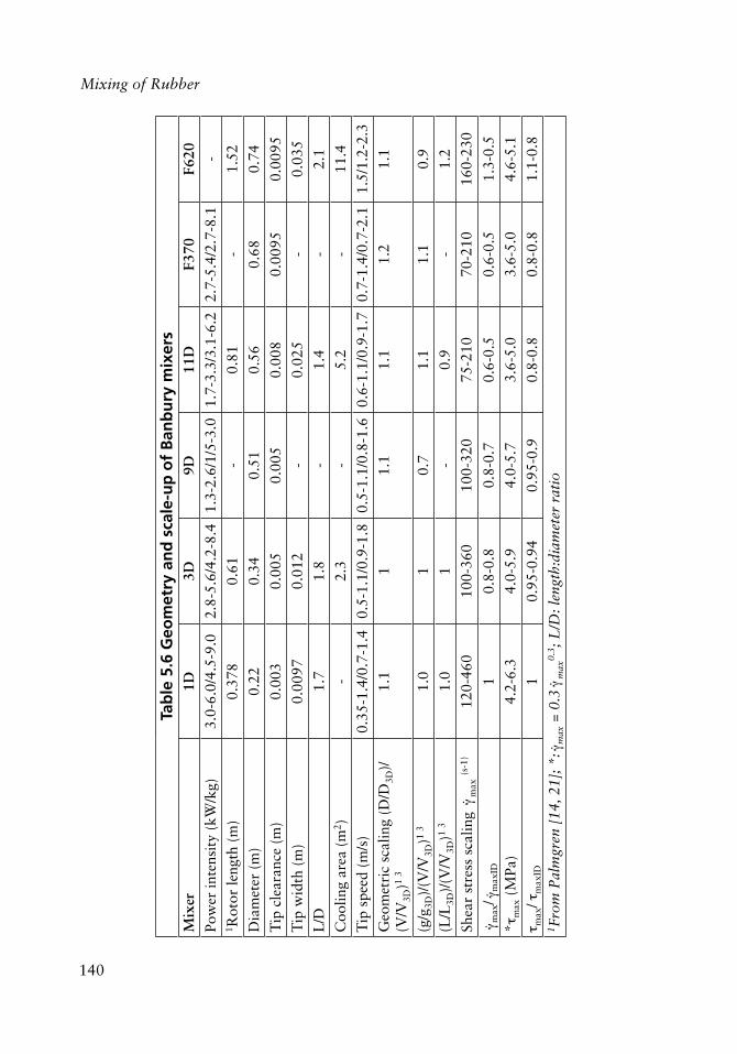
140

Mixing of Rubber

Tab

le 5

.6 G

eom

etry

an

d s

cale

-up

of

Ban

bu

ry m

ixer

sM

ixer

1D3D

9D11

DF3

70F6

20Po

wer

inte

nsit

y (k

W/k

g)3.

0-6.

0/4.

5-9.

02.

8-5.

6/4.

2-8.

41.

3-2.

6/1/

5-3.

01.

7-3.

3/3.

1-6.

22.

7-5.

4/2.

7-8.

1-

1 Rot

or le

ngth

(m

)0.

378

0.61

-0.

81-

1.52

Dia

met

er (

m)

0.22

0.34

0.51

0.56

0.68

0.74

Tip

cle

aran

ce (

m)

0.00

30.

005

0.00

50.

008

0.00

950.

0095

Tip

wid

th (

m)

0.00

970.

012

-0.

025

-0.

035

L/D

1.7

1.8

-1.

4-

2.1

Coo

ling

area

(m

2 )-

2.3

-5.

2-

11.4

Tip

spe

ed (

m/s

)0.

35-1

.4/0

.7-1

.40.

5-1.

1/0.

9-1.

80.

5-1.

1/0.

8-1.

60.

6-1.

1/0.

9-1.

70.

7-1.

4/0.

7-2.

11.

5/1.

2-2.

3

Geo

met

ric

scal

ing

(D/D

3D)/

(V/V

3D)1

31.

11

1.1

1.1

1.2

1.1

(g/g

3D)/

(V/V

3D)1

31.

01

0.7

1.1

1.1

0.9

(L/L

3D)/

(V/V

3D)1

31.

01

-0.

9-

1.2

Shea

r st

ress

sca

ling

� �m

ax (s

-1)

120-

460

100-

360

100-

320

75-2

1070

-210

160-

230

� �m

ax/ � �

max

ID1

0.8-

0.8

0.8-

0.7

0.6-

0.5

0.6-

0.5

1.3-

0.5

*�m

ax (

MPa

)4.

2-6.

34.

0-5.

94.

0-5.

73.

6-5.

03.

6-5.

04.

6-5.

1

� max

/ �m

axID

10.

95-0

.94

0.95

-0.9

0.8-

0.8

0.8-

0.8

1.1-

0.8

1 Fro

m P

alm

gren

[14

, 21]

; *: � �

max

= 0

.3 � �

max

0.3 ;

L/D

: len

gth:

diam

eter

rat

io

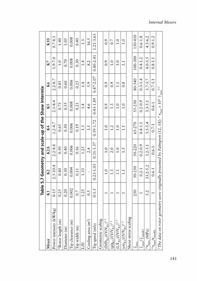
141

Internal Mixers

Tab

le 5

.7 G

eom

etry

an

d s

cale

-up

of

the

Shaw

Inte

rmix

Mix

erK

1K

2K

2AK

4K

5K

6K

7K

10Po

wer

inte

nsit

y (k

W/k

g)0-

152.

5-10

.42.

2-8.

81.

2-4.

72.

1-8.

42.

2-8.

71.

9-7.

00.

7-8.

11 R

otor

leng

th (

m)

0.25

0.40

0.50

0.65

0.75

0.85

1.0

1.40

Dia

met

er (

m)

0.20

0.30

0.40

0.50

0.55

0.60

0.70

1.05

Tip

cle

aran

ce (

m)

0.00

20.

004

0.00

60.

006

0.00

80.

006

0.00

80.

008

Tip

wid

th (

m)

0.7

0.11

0.16

0.19

0.21

0.25

0.30

0.40

L/D

1.25

1.33

1.25

1.3

1.4

1.4

1.4

1.3

Coo

ling

area

(m

2 )0.

5-

2.4

3.5

4.6

5.9

8.2

16.5

Tip

spe

ed (

m/s

)0-

1.5

0.23

-1.0

30.

31-1

.37

0.39

-1.7

20.

43-1

.89

0.47

-2.0

70.

80-2

.41

1.21

-3.6

3

Geo

met

ric

scal

ing

(D/D

K1)

/(V

/VK

1)1

31

1.0

1.0

1.0

0.9

0.9

0.9

0.9

(g/g

K1)

/(V

/VK

1)1

31

1.3

2.0

1.2

1.3

0.9

1.0

0.7

(L/L

K1)

/(V

/VK

1)1

31

1.1

1.0

1.0

1.0

1.1

1.0

1.0

(e/e

K1)

/(V

/VK

1)1

31

1.1

1.5

1.1

1.0

0.8

1.1

1.0

Shea

r st

ress

sca

ling

� �m

ax25

050

-250

50-2

2065

-270

55-2

3080

-340

100-

300

150-

450

� �m

ax/ � �

max

K1

10.

2-1

0.2-

0.9

0.4-

1.1

0.2-

0.9

0.3-

1.4

0.4-

1.2

0.6-

1.8

*�m

ax (

MPa

)5.

233

.2-5

.23.

2-5.

13.

5-5.

43.

3-5.

13.

7-5.

74.

0-5.

54.

5-6.

2

*�m

ax/�

max

/1

10.

6-1

0.6-

10.

7-1

0.6-

10.

7-1.

10.

8-1.

10.

9-1.

21 T

he d

ata

on r

otor

geo

met

ry w

ere

orig

inal

ly p

rese

nted

by

Pal

mgr

en [

12, 1

8]; *

�m

ax =

105

� �m

ax0.

3

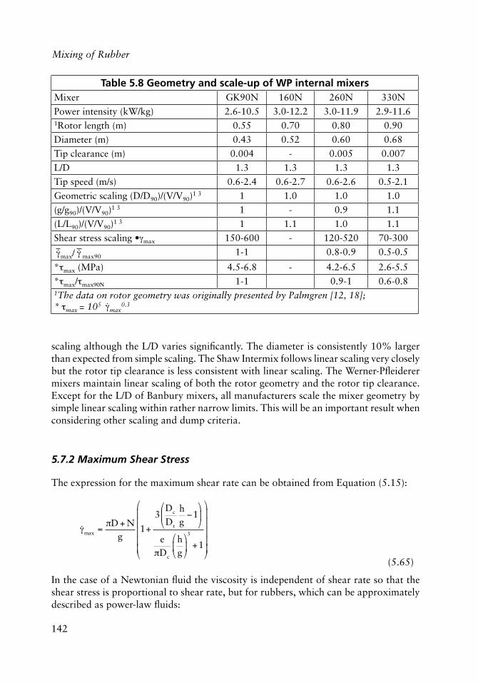
142

Mixing of Rubber

scaling although the L/D varies signifi cantly. The diameter is consistently 10% larger than expected from simple scaling. The Shaw Intermix follows linear scaling very closely but the rotor tip clearance is less consistent with linear scaling. The Werner-Pfl eiderer mixers maintain linear scaling of both the rotor geometry and the rotor tip clearance. Except for the L/D of Banbury mixers, all manufacturers scale the mixer geometry by simple linear scaling within rather narrow limits. This will be an important result when considering other scaling and dump criteria.

5.7.2 Maximum Shear Stress

The expression for the maximum shear rate can be obtained from Equation (5.15):

��max =�D + N

g1+

3Dc

Dt

hg�1

�

��

�

��

e�Dc

hg

�

��

�

��

3

+1

�

�

��

�

�

��

(5.65)

In the case of a Newtonian fl uid the viscosity is independent of shear rate so that the shear stress is proportional to shear rate, but for rubbers, which can be approximately described as power-law fl uids:

Table 5.8 Geometry and scale-up of WP internal mixersMixer GK90N 160N 260N 330N

Power intensity (kW/kg) 2.6-10.5 3.0-12.2 3.0-11.9 2.9-11.61Rotor length (m) 0.55 0.70 0.80 0.90

Diameter (m) 0.43 0.52 0.60 0.68

Tip clearance (m) 0.004 - 0.005 0.007

L/D 1.3 1.3 1.3 1.3

Tip speed (m/s) 0.6-2.4 0.6-2.7 0.6-2.6 0.5-2.1

Geometric scaling (D/D90)/(V/V90)1 3 1 1.0 1.0 1.0

(g/g90)/(V/V90)1 3 1 - 0.9 1.1

(L/L90)/(V/V90)1 3 1 1.1 1.0 1.1

Shear stress scaling •�max 150-600 - 120-520 70-300

��max/ �� max90 1-1 0.8-0.9 0.5-0.5

*�max (MPa) 4.5-6.8 - 4.2-6.5 2.6-5.5

*�max/�max902 1-1 0.9-1 0.6-0.81The data on rotor geometry was originally presented by Palmgren [12, 18]; * �max = 105

��max

0.3

143

Internal Mixers

�max = k��max

n

(5.66)

where n =1.0 for Newtonian fl uids but more typically n = 0.2 - 0.4 for fi lled rubbers.

For a complete analysis, the pressure fl ow term should be included in the equation but data on the channel diameter Dc and channel gap h are not generally available. As an estimate for Banbury rotors, and using the dimensions for a 3D machine:

Dc ~ 0.75 Dt

h ~ 0.25 Dt

3DchDt

�

��

�

�� g

eh3

�g2Dc

+ g= 0.5

(5.67)

Thus the pressure term increases the maximum shear rate by approximately 50% compared to the term for drag fl ow alone. Because the mixers for anyone manufacturer are nearly geometrically similar, the pressure fl ow contribution will be nearly a constant factor. Because we are only interested in ratios of maximum shear rates or shear stresses between machines for the scale-up problem, the maximum shear rate can be calculated using the drag fl ow term only:

�� =

�DtNg

(5.68)

This is the expression used to calculate the maximum shear rates reported in Tables 5.6-5.8. The pressure fl ow term must be included in the analysis of a single mixer, as developed in Section 5.2 and Section 5.3. The maximum shear stress can be calculated from the maximum shear rate using Equation (5.66). As a typical set of constants for illustrating scale-up, the expression:

�max = 1�105

��max0.3

(5.69)

was used to calculate the values in Tables 5.6-5.8.

The ratio of maximum shear rates equals the ratio of maximum shear stresses for scale-up of a Newtonian fl uid. It can be seen that the maximum shear rate (or shear stress if Newtonian fl uid) varies widely from one machine to another. High pressure-high speed operation increases the shear rate by as much as a factor of four for anyone machine, but for the same mode of operation, the maximum shear rate is smaller for larger machines with the exception of the Shaw Intermix K10. If the maximum shear stress is calculated according to Equation (5.69), the variation in maximum shear stress is much smaller.

144

Mixing of Rubber

The maximum stress does not depend upon machine size although it is approximately 50% larger in the high speed mode.

For a pair of machines with fi xed geometries, the maximum shear stress could be maintained constant if:

Dt1N1

g1

�

��

�

��

n

=Dt2N2

g2

�

��

�

��

n

(5.70)

N2

N1

=g2

g1

Dt1

Dt2 (5.71)

which means that the rotor speeds for the two machines should be the same, if they were strictly geometrically similar. If commercial machines had adjustable rotor speeds, the scale-up relation in Equation (5.71) could be used to maintain a constant shear stress. However, diffi culties in mechanical construction restrict the choice of rotor speeds and the maximum shear stress is not constant when a process is transferred from one machine to another.

For many mixing problems, the change in maximum shear stress would not be a serious diffi culty if the temperature history of the rubber was the same so at any point in the cycle the viscosity would be the same in the two mixers. Because the viscosity is temperature dependent, the expression in Equation (5.66) becomes:

�max = A exp b T To( )( ) ��max

n

(5.72)

In scale-up, the temperature history in two mixers may be signifi cantly different, as will be discussed in Section 5.8, so that the maximum shear stress may be signifi cantly lower than expected from the data in Tables 5.6-5.8 in a larger machine if it is operating at 10-20 °C higher temperature.

As long as the shear stress is above the critical stress required for particle dispersion, the value does not matter and a constant total shear strain criterion should be used. However, if because of geometry or temperature effects the maximum stress falls below the critical stress, then particles will not be dispersed. Both cases can be observed when transferring a process from the laboratory to the plant. In most cases where particle break-up is incomplete, the large scale machine has fi xed geometry and rotor speeds. The only way that the maximum shear stress can be increased for the same rubber recipe is to lower the mixing temperature.

145

Internal Mixers

5.7.3 Total Shear Strain

Transferring the mixing from one machine to another while maintaining a constant total shear strain sets the mixing time once the mixer geometry and rotor speed are known. Because of the pressure fl ow term, the total shear generated per rotor revolution contains implicitly the rate of rotation and the material properties as shown in Equations (5.9)-(5.11). Even for the ideal rotor geometry considered in that model, explicit expressions for the total strain become unwieldy. In the conditions of real mixers, only numerical solutions are possible. However, for a series of similar mixers approximations such as described in the previous section can be used. If the pressure fl ow term makes a proportional contribution to the shear rate such that:

�� = ��d + ��p = 1+ a( ) ��d

(5.73)

for fl ow between the rotor tip and the chamber wall as well as between the rotor shafts and the rotor shaft and chamber walls, then the approximations leading to Equation (5.35) can be used:

�� =

e�Dc

��t + 1 =e

�Dc

�

��

�

� ��c

(5. 35b)

and

��c

��t

�Dc

Dt

gh

(5.34)

so that:

��t

=e

�Dc

+ 1�e

�Dc

�

��

�

��Dc

Dt

gh

= b

and the total shear strain is proportional to the shear rate at the rotor tip.

� = ��tm = b��ttm

(5.74)

where:

tm = mixing time

For a series of geometrically similar machines, the parameter b will be a constant and the ratio of total shear strains will be proportional to the ratio of shear strains generated at the tip.

146

Mixing of Rubber

If only drag fl ow is considered:

��t =

�DtNg

= ��max

(5.75)

and the ratio of mixing times is given by:

tm2

tm2

=��max1

��max2 (5.76)

These ratios have been tabulated in Tables 5.6 - 5.8. It can be seen that for a given mixer, high pressure-high speed mode of operation increases the shear rate by 3-5 times so that the mixing time can be reduced by a similar amount compared to the low pressure process. This agrees well with the observations reported in Section 5.5.

Van Buskirk and co-workers [2] implicitly used these assumptions in calculating the total shear strain as:

� =

2.15Vb

eDtLNt

(5.77)

Approximating the batch volume by:

Vb = �Dcgh

it can readily be seen that this equals the total shear calculated by:

� =

e�Dc

��ttm

(5.78)

which is the shear strain generated by the rotor tip. The relative weight of the shear strain generated in the channel versus the strain generated at the tip can be calculated from Equation (5.35):

�c

�t

=

1�e

�Dc

�

��

�

��Dc

Dt

gh

e�Dc

=�Dc

e�1

�

��

�

��Dc

Dt

gh

(5.79)

For the Banbury 11D, using the approximations:

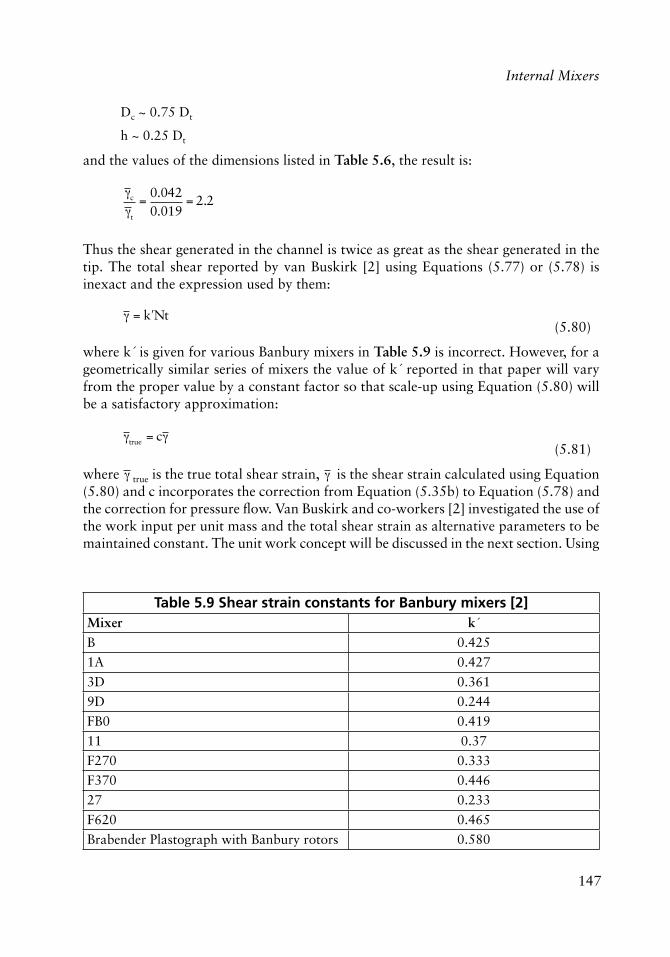
147

Internal Mixers

Dc ~ 0.75 Dt

h ~ 0.25 Dt

and the values of the dimensions listed in Table 5.6, the result is:

�c

�t

=0.0420.019

= 2.2

Thus the shear generated in the channel is twice as great as the shear generated in the tip. The total shear reported by van Buskirk [2] using Equations (5.77) or (5.78) is inexact and the expression used by them:

� = �k Nt

(5.80)

where k´ is given for various Banbury mixers in Table 5.9 is incorrect. However, for a geometrically similar series of mixers the value of k´ reported in that paper will vary from the proper value by a constant factor so that scale-up using Equation (5.80) will be a satisfactory approximation:

�true = c�

(5.81)

where � true is the true total shear strain, � is the shear strain calculated using Equation (5.80) and c incorporates the correction from Equation (5.35b) to Equation (5.78) and the correction for pressure fl ow. Van Buskirk and co-workers [2] investigated the use of the work input per unit mass and the total shear strain as alternative parameters to be maintained constant. The unit work concept will be discussed in the next section. Using

Table 5.9 Shear strain constants for Banbury mixers [2]Mixer k´B 0.425

1A 0.427

3D 0.361

9D 0.244

FB0 0.419

11 0.37

F270 0.333

F370 0.446

27 0.233

F620 0.465

Brabender Plastograph with Banbury rotors 0.580

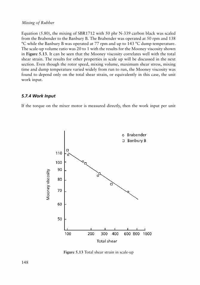
148

Mixing of Rubber

Equation (5.80), the mixing of SBR1712 with 50 phr N-339 carbon black was scaled from the Brabender to the Banbury B. The Brabender was operated at 50 rpm and 138 °C while the Banbury B was operated at 77 rpm and up to 143 °C dump temperature. The scale-up volume ratio was 20 to 1 with the results for the Mooney viscosity shown in Figure 5.13. It can be seen that the Mooney viscosity correlates well with the total shear strain. The results for other properties in scale up will be discussed in the next section. Even though the rotor speed, mixing volume, maximum shear stress, mixing time and dump temperature varied widely from run to run, the Mooney viscosity was found to depend only on the total shear strain, or equivalently in this case, the unit work input.

5.7.4 Work Input

If the torque on the mixer motor is measured directly, then the work input per unit

Figure 5.13 Total shear strain in scale-up

149

Internal Mixers

volume can be calculated:

dW = dP / Vb

=2�N 9.8�10�6( )

Vb

T(t)dt

W =2�N 9.8�10�6( )

Vb

T(t)dt� (5.82)

where N is the rotor speed in rpm, T(t) is the measured torque in m-kg, t is the time minutes and Vb is the batch volume in m3 to give the work input W in MJ/m3. The recorder trace can be integrated graphically or the torque transducer output can be integrated electronically for experimentally-measured torque-time curves.

The measured torque is related to the shear stress at the rotor wall by Equation (5.16):

T = s � t,y=0

eDt

z+ �y=0 Dc = e( ) Dc

z

�

��

�

��

(5.16)

The shear rate in the channel is related to that at the tip by Equation (5.35):

��c

��t

=Dc

Dt

gh

~ 0.05

for many mixers. If the material is Newtonian, then:

T = � ��

and Equation (5.16) becomes:

T =�s ��teDt

2+ ��c �Dc � e( ) Dc

2

�

��

�

��

=�Dc�s��t

2e�

Dt

Dc

+��c

��t

1�e

Dc

�

��

�

��Dc

�

��

�

��

(5.83)

TVb

=T

�Dcgs

=��t

2ge�

Dt

Dc

+��c

��t

1�e

�Dc

�

��

�

��Dc

�

��

�

��

(5.84)

150

Mixing of Rubber

if the material behaves as a power-law fl uid, the expression becomes:

TVb

=k��t

n

2geDt

�Dc

+��c

��t

�

��

�

��

n

1�e

�Dc

�

��

�

��Dc

�

�

��

�

�

��

(5.85)

The ratio of shear rates depends only upon the geometry so that the work input can be calculated:

W =2�Vb

T t( ) Ndt�

= 2�kN��t

n

2geDt

�Dc

+��c

��t

�

�

�

�

n

1�e

�Dc

�

�

�

�Dc

�

�

�

��

(5.86)

Substituting Equations (5.68) and (5.78) yields:

W = 2�k

2�0

tm

� �tm

��tn 1+

��c

��

�

�

�

�

n�Dc

e�1

�

�

�

�Dc

Dt

�

�

�

��

=�

tm

k��tn 1+

��c

��t

�

�

�

�

n�Dc

e�1

�

�

�

�Dc

Dt

�

�

�

��

0

tm

� dt

(5.87)

W = b�

and

log W = log y + b (5.88)

where b is the time-average of the integrand in Equation (5.87). This is the same as the equation derived empirically by van Buskirk [2] from experimental torque measurements and shear strain calculated using Equation (5.80). The integral in Equation (5.87) depends upon the geometry of the mixer, the rotor speed and the temperature-history of the material through the temperature dependence of viscosity.

In practice, the approximations leading to Equation (5.78) for the calculation of shear rate necessitate the introduction of another factor:

log W = a log � + log b (5.89)

where a is close to one for most systems.

If the temperature history of a material in two mixers is similar, then the difference between scaling at constant shear strain or scaling at constant work input may be diffi cult to discern. If the work input is calculated from direct rotor torque measurements, this

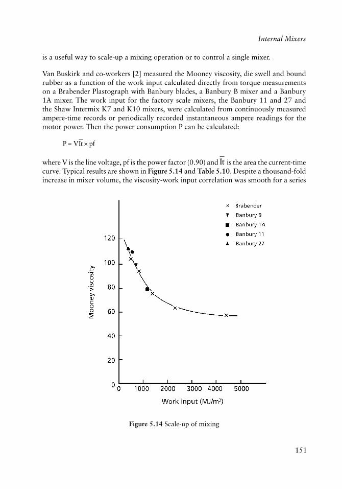
151

Internal Mixers

is a useful way to scale-up a mixing operation or to control a single mixer.

Van Buskirk and co-workers [2] measured the Mooney viscosity, die swell and bound rubber as a function of the work input calculated directly from torque measurements on a Brabender Plastograph with Banbury blades, a Banbury B mixer and a Banbury 1A mixer. The work input for the factory scale mixers, the Banbury 11 and 27 and the Shaw Intermix K7 and K10 mixers, were calculated from continuously measured ampere-time records or periodically recorded instantaneous ampere readings for the motor power. Then the power consumption P can be calculated:

P = VIt � pf

where V is the line voltage, pf is the power factor (0.90) and It is the area the current-time curve. Typical results are shown in Figure 5.14 and Table 5.10. Despite a thousand-fold increase in mixer volume, the viscosity-work input correlation was smooth for a series

Figure 5.14 Scale-up of mixing

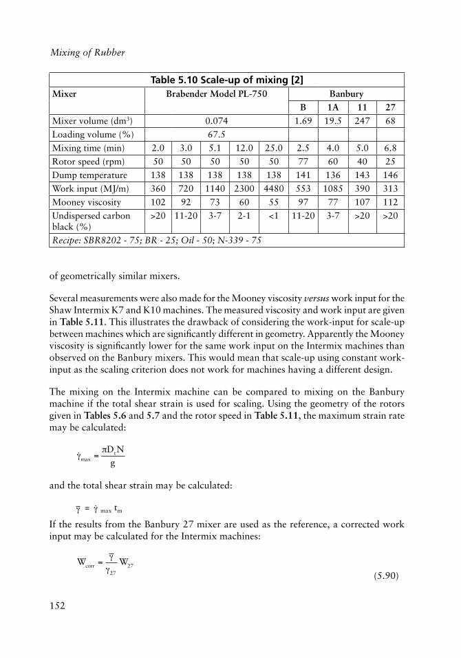
152

Mixing of Rubber

of geometrically similar mixers.

Several measurements were also made for the Mooney viscosity versus work input for the Shaw Intermix K7 and K10 machines. The measured viscosity and work input are given in Table 5.11. This illustrates the drawback of considering the work-input for scale-up between machines which are signifi cantly different in geometry. Apparently the Mooney viscosity is signifi cantly lower for the same work input on the Intermix machines than observed on the Banbury mixers. This would mean that scale-up using constant work-input as the scaling criterion does not work for machines having a different design.

The mixing on the Intermix machine can be compared to mixing on the Banbury machine if the total shear strain is used for scaling. Using the geometry of the rotors given in Tables 5.6 and 5.7 and the rotor speed in Table 5.11, the maximum strain rate may be calculated:

��max =

�DtNg

and the total shear strain may be calculated:

� = �� max tm

If the results from the Banbury 27 mixer are used as the reference, a corrected work input may be calculated for the Intermix machines:

Wcorr =

��27

W27

(5.90)

Table 5.10 Scale-up of mixing [2]Mixer Brabender Model PL-750 Banbury

B 1A 11 27Mixer volume (dm3) 0.074 1.69 19.5 247 68

Loading volume (%) 67.5

Mixing time (min) 2.0 3.0 5.1 12.0 25.0 2.5 4.0 5.0 6.8

Rotor speed (rpm) 50 50 50 50 50 77 60 40 25

Dump temperature 138 138 138 138 138 141 136 143 146

Work input (MJ/m) 360 720 1140 2300 4480 553 1085 390 313

Mooney viscosity 102 92 73 60 55 97 77 107 112

Undispersed carbon black (%)

>20 11-20 3-7 2-1 <1 11-20 3-7 >20 >20

Recipe: SBR8202 - 75; BR - 25; Oil - 50; N-339 - 75

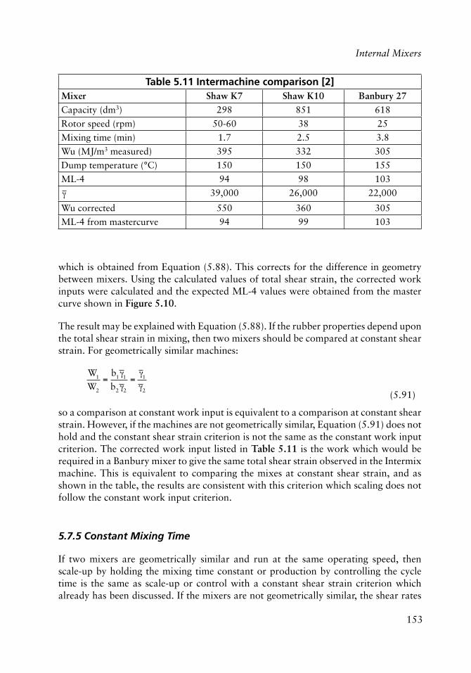
153

Internal Mixers

which is obtained from Equation (5.88). This corrects for the difference in geometry between mixers. Using the calculated values of total shear strain, the corrected work inputs were calculated and the expected ML-4 values were obtained from the master curve shown in Figure 5.10.

The result may be explained with Equation (5.88). If the rubber properties depend upon the total shear strain in mixing, then two mixers should be compared at constant shear strain. For geometrically similar machines:

W1

W2

=b1�1b2 �2

=�1�2

(5.91)

so a comparison at constant work input is equivalent to a comparison at constant shear strain. However, if the machines are not geometrically similar, Equation (5.91) does not hold and the constant shear strain criterion is not the same as the constant work input criterion. The corrected work input listed in Table 5.11 is the work which would be required in a Banbury mixer to give the same total shear strain observed in the Intermix machine. This is equivalent to comparing the mixes at constant shear strain, and as shown in the table, the results are consistent with this criterion which scaling does not follow the constant work input criterion.

5.7.5 Constant Mixing Time

If two mixers are geometrically similar and run at the same operating speed, then scale-up by holding the mixing time constant or production by controlling the cycle time is the same as scale-up or control with a constant shear strain criterion which already has been discussed. If the mixers are not geometrically similar, the shear rates

Table 5.11 Intermachine comparison [2]Mixer Shaw K7 Shaw K10 Banbury 27Capacity (dm3) 298 851 618

Rotor speed (rpm) 50-60 38 25

Mixing time (min) 1.7 2.5 3.8

Wu (MJ/m3 measured) 395 332 305

Dump temperature (°C) 150 150 155

ML-4 94 98 103

� 39,000 26,000 22,000

Wu corrected 550 360 305

ML-4 from mastercurve 94 99 103

154

Mixing of Rubber

may be considerably different, even at the same rotor speed so that the mixing time is not a reliable measure for scale-up. If the rotor speeds in two dissimilar mixers are in proportion, so that shear rate is the same in both machines, then the constant mixing time criterion is the same as the constant total shear criterion.

One possible diffi culty in using the cycle time as the control variable in a mixing operation is that the effective mixing time may be less than the total mixing time, particularly in low pressure mixers. In this operation, the rubber is not immediately drawn into the rotors because of slip at the wall, as discussed in Section 5.5. If this occurs, very little shear will be generated until fl ow commences. The length of the induction period will depend upon stock temperature, mixer temperature, rotor speed and other variables. Generally, the induction time will vary from batch to batch so that the effective mixing time will vary and the cycle time will not be a measure of the mixing time. In high pressure-high speed processes, this induction period is essentially eliminated so that cycle time does correspond to effective mixing time.

In the high pressure process, controlling at a constant cycle time corresponds to controlling at a constant mixing time, hence a constant shear strain when the rotor speed is constant for a single machine. Because of this simple correspondence, it was found that the Polymer-Physik Controller [22] which integrates the power to the motor to give the work input as a control variable did not improve the performance on a Banbury mixer compared to cycle time as the control variable. In the low pressure process where slip can be signifi cant, the controller may be expected to improve performance compared to the mixing time criterion.

If the geometry and rotor speeds are known for two mixers, so that the shear rates can be calculated, then the mixing time in scale-up can be calculated:

tm2

tm1

=��1

��2 (5.92)

Unless the ratio of shear rates in the two machines is known, the simple criterion of constant mixing time may be inadequate.

5.7.6 Constant Stock Temperature

The energy balance for an internal mixer was discussed in Section 5.4. The net motor work is dissipated in the rubber from viscous losses to generate heat. Some of this energy is conducted away by the cooling water and some of the energy raises the temperature of the stock and the machine walls. The rate of energy dissipation is a function of the shear rate. If two mixes are prepared at the same total shear strain but at two different shear rates, the higher shear rate material will generate more heat. In additions the contact time with the cooling walls will be less so that less heat will be conducted away at the

155

Internal Mixers

higher shear rate. Consequently the average stock temperature will be higher in the high rate mix for the same external cooling conditions. Alternatively, the temperature of the stock can be lowered for the same shear rate and mixing time by using chilled water. Thus the stock temperature can be controlled, at least within limits, independently of the work input or total shear strain. As can be seen in Table 5.11, the stock temperature at dump bears no relationship to the mix properties.

As seen in Tables 5.6 and 5.7, the cooling area-to-mixer volume ratio decreases rapidly for larger mixers. Consequently the rate of heat transfer decreases relative to the rate of heat generation for the same shear rate and the stock temperature will be higher for larger machines. If there is a maximum stock temperature because of scorchiness with curing additives, then the larger machine must be operated at a lower shear rate, hence longer mixing time, than the smaller machine. The relation in scale-up can be derived from the model given in Section 5.2 and Section 5.4. The higher stock temperature for larger machines may also be a problem if the temperature-dependence of viscosity lowers the maximum shear stress below the critical value for particle dispersion.

5.7.7 Constant Weissenberg and Deborah Numbers

One major limitation to internal mixer operation is the appearance of fl ow instabilities similar to those discussed for roll mills in Chapter 4. Region 1 behaviour where slip occurs at the wall in drag fl ow can delay the start of effective mixing by preventing fl ow between the rotors and the rotors and the wall. This problem is overcome by using higher ram pressures as discussed earlier. Region 2 and region 4 are both stable fl ow regimes but region 2 gives better dispersion because of a larger elongational stress which is more effective in agglomerate dispersion than is a shear stress. Region 3 gives poor mixing because a signifi cant portion of the stock forms crumbs with a ‘cheesy’ consistency [23]. The material behaves as if melt fracture occurs and there is plug fl ow in the high stress region rather than shearing fl ow. Consequently the dispersion is signifi cantly lower.

Another type of instability is also possible. When a pressure transducer is placed in the chamber wall with a Newtonian material it is observed that pressure rises as the rotor tip passes the transducer, then quickly returns to the baseline pressure. With viscoelastic materials, the stress relaxes slowly so that the pressure decays slowly. If the rotor speed is too high, then the material will not relax between subsequent passes so that the shear stress will increased for the imposed shear rate. The material is effectively pre-stressed before passing through the nip. If the pre-stress is great enough, then the shear stress at the wall will exceed the critical stress for slip and the rubber will not pass through the gap between the rotor tip and the chamber wall. This behaviour looks like a region 1 fl ow, but the onset of instability is controlled by a critical Deborah number rather than Weissenberg number.

Unfortunately, insuffi cient evidence is available to assign quantitative values to the critical

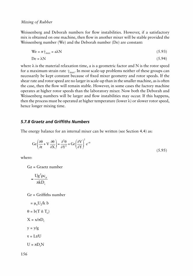
156

Mixing of Rubber

Weissenberg and Deborah numbers for fl ow instabilities. However, if a satisfactory mix is obtained on one machine, then fl ow in another mixer will be stable provided the Weissenberg number (We) and the Deborah number (De) are constant:

We = � ��max = a%N (5.93)

De = %N (5.94)

where % is the material relaxation time, a is a geometric factor and N is the rotor speed for a maximum strain rate

��max. In most scale-up problems neither of these groups can

necessarily be kept constant because of fi xed mixer geometry and rotor speeds. If the shear rate and rotor speed are no larger in scale-up than in the smaller machine, as is often the case, then the fl ow will remain stable. However, in some cases the factory machine operates at higher rotor speeds than the laboratory mixer. Now both the Deborah and Weissenberg numbers will be larger and fl ow instabilities may occur. If this happens, then the process must be operated at higher temperature (lower %) or slower rotor speed, hence longer mixing time.

5.7.8 Graetz and Griffi ths Numbers

The energy balance for an internal mixer can be written (see Section 4.4) as:

Gz

��t

+ V��X

�

��

�

�� =

�2�

�Y2+ Gr

�V�Y

�

��

�

��

2

e��

(5.95)

where:

Gz = Graetz number

=

Ug2�cp

�kDt

Gr = Griffi ths number

= �oU2/k b

* = b(T ñ To)

X = x/�Dt

y = y/g

� = Lt/U

U = �DtN

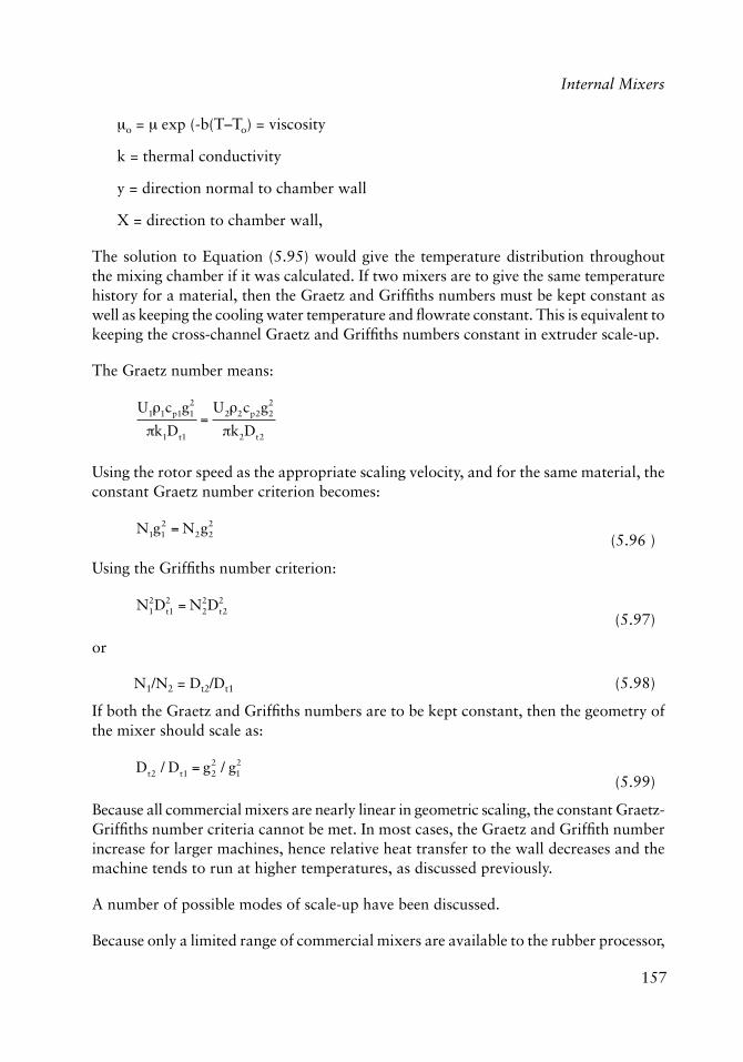
157

Internal Mixers

�o = � exp (-b(T–To) = viscosity

k = thermal conductivity

y = direction normal to chamber wall

X = direction to chamber wall,

The solution to Equation (5.95) would give the temperature distribution throughout the mixing chamber if it was calculated. If two mixers are to give the same temperature history for a material, then the Graetz and Griffi ths numbers must be kept constant as well as keeping the cooling water temperature and fl owrate constant. This is equivalent to keeping the cross-channel Graetz and Griffi ths numbers constant in extruder scale-up.

The Graetz number means:

U1�1cp1g12

�k1Dt1

=U2�2cp2g2

2

�k2Dt2

Using the rotor speed as the appropriate scaling velocity, and for the same material, the constant Graetz number criterion becomes:

N1g1

2 = N2g22

(5.96 )

Using the Griffi ths number criterion:

N1

2Dt12 = N2

2Dt22

(5.97)

or

N1/N2 = Dt2/Dt1 (5.98)

If both the Graetz and Griffi ths numbers are to be kept constant, then the geometry of the mixer should scale as:

Dt2 / Dt1 = g2

2 / g12

(5.99)

Because all commercial mixers are nearly linear in geometric scaling, the constant Graetz-Griffi ths number criteria cannot be met. In most cases, the Graetz and Griffi th number increase for larger machines, hence relative heat transfer to the wall decreases and the machine tends to run at higher temperatures, as discussed previously.

A number of possible modes of scale-up have been discussed.

Because only a limited range of commercial mixers are available to the rubber processor,

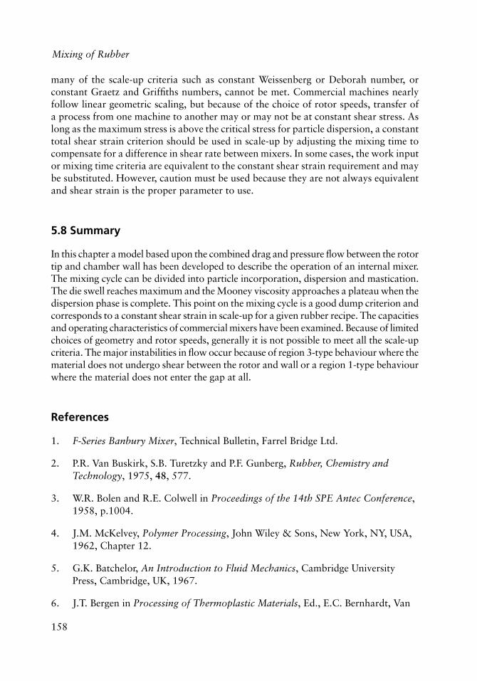
158

Mixing of Rubber

many of the scale-up criteria such as constant Weissenberg or Deborah number, or constant Graetz and Griffi ths numbers, cannot be met. Commercial machines nearly follow linear geometric scaling, but because of the choice of rotor speeds, transfer of a process from one machine to another may or may not be at constant shear stress. As long as the maximum stress is above the critical stress for particle dispersion, a constant total shear strain criterion should be used in scale-up by adjusting the mixing time to compensate for a difference in shear rate between mixers. In some cases, the work input or mixing time criteria are equivalent to the constant shear strain requirement and may be substituted. However, caution must be used because they are not always equivalent and shear strain is the proper parameter to use.

5.8 Summary

In this chapter a model based upon the combined drag and pressure fl ow between the rotor tip and chamber wall has been developed to describe the operation of an internal mixer. The mixing cycle can be divided into particle incorporation, dispersion and mastication. The die swell reaches maximum and the Mooney viscosity approaches a plateau when the dispersion phase is complete. This point on the mixing cycle is a good dump criterion and corresponds to a constant shear strain in scale-up for a given rubber recipe. The capacities and operating characteristics of commercial mixers have been examined. Because of limited choices of geometry and rotor speeds, generally it is not possible to meet all the scale-up criteria. The major instabilities in fl ow occur because of region 3-type behaviour where the material does not undergo shear between the rotor and wall or a region 1-type behaviour where the material does not enter the gap at all.

References

1. F-Series Banbury Mixer, Technical Bulletin, Farrel Bridge Ltd.

2. P.R. Van Buskirk, S.B. Turetzky and P.F. Gunberg, Rubber, Chemistry and Technology, 1975, 48, 577.

3. W.R. Bolen and R.E. Colwell in Proceedings of the 14th SPE Antec Conference, 1958, p.1004.

4. J.M. McKelvey, Polymer Processing, John Wiley & Sons, New York, NY, USA, 1962, Chapter 12.

5. G.K. Batchelor, An Introduction to Fluid Mechanics, Cambridge University Press, Cambridge, UK, 1967.

6. J.T. Bergen in Processing of Thermoplastic Materials, Ed., E.C. Bernhardt, Van

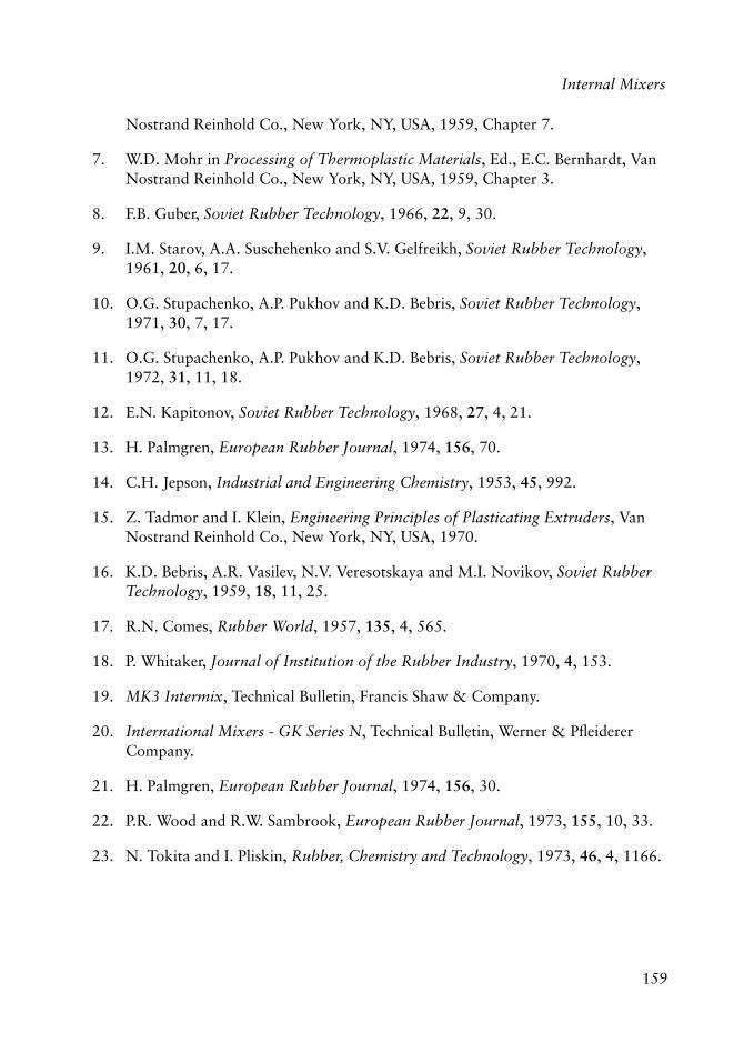
159

Internal Mixers

Nostrand Reinhold Co., New York, NY, USA, 1959, Chapter 7.

7. W.D. Mohr in Processing of Thermoplastic Materials, Ed., E.C. Bernhardt, Van Nostrand Reinhold Co., New York, NY, USA, 1959, Chapter 3.

8. F.B. Guber, Soviet Rubber Technology, 1966, 22, 9, 30.

9. I.M. Starov, A.A. Suschehenko and S.V. Gelfreikh, Soviet Rubber Technology, 1961, 20, 6, 17.

10. O.G. Stupachenko, A.P. Pukhov and K.D. Bebris, Soviet Rubber Technology, 1971, 30, 7, 17.

11. O.G. Stupachenko, A.P. Pukhov and K.D. Bebris, Soviet Rubber Technology, 1972, 31, 11, 18.

12. E.N. Kapitonov, Soviet Rubber Technology, 1968, 27, 4, 21.

13. H. Palmgren, European Rubber Journal, 1974, 156, 70.

14. C.H. Jepson, Industrial and Engineering Chemistry, 1953, 45, 992.

15. Z. Tadmor and I. Klein, Engineering Principles of Plasticating Extruders, Van Nostrand Reinhold Co., New York, NY, USA, 1970.

16. K.D. Bebris, A.R. Vasilev, N.V. Veresotskaya and M.I. Novikov, Soviet Rubber Technology, 1959, 18, 11, 25.

17. R.N. Comes, Rubber World, 1957, 135, 4, 565.

18. P. Whitaker, Journal of Institution of the Rubber Industry, 1970, 4, 153.

19. MK3 Intermix, Technical Bulletin, Francis Shaw & Company.

20. International Mixers - GK Series N, Technical Bulletin, Werner & Pfl eiderer Company.

21. H. Palmgren, European Rubber Journal, 1974, 156, 30.

22. P.R. Wood and R.W. Sambrook, European Rubber Journal, 1973, 155, 10, 33.

23. N. Tokita and I. Pliskin, Rubber, Chemistry and Technology, 1973, 46, 4, 1166.

160

Mixing of Rubber

161

Continuous Mixers

Continuous Mixers

AuthorAuthor 6Many mixing lines use an extruder to form strand, sheet, slab or pellets from the dumped stock of an internal mixer. Although some laminar shear mixing does occur in these extruders, they are primarily designed to alter the shape of the materials for subsequent use and the mixing which occurs is secondary. The design and operation of these machines is beyond the scope of this text.

In a number of product lines, mixing is achieved in two steps. Carbon black and other inert ingredients are added in the fi rst stage internal mixer which incorporates the fi ller and partially disperses the particles. The incompletely mixed material is dumped from the mixer onto a mill or extruder to shape the stock, which is then allowed to cool. Vulcanising agents are added to the stock in a second mixer which completes the particle dispersion while the temperature-history of the active ingredients is held to a lower heat level to prevent scorching. In many cases internal mixers are used for both mixing steps. However, it is often possible to replace one or both internal mixers by a continuous mixer.

6.1 Mixing in Single Screw Extruders

Among the earliest analyses of fl ow in conventional single screw extruders is that developed by Carley, McKelvey and co-workers [1-3]. Mohr, Saxton and Jepson [4, 5] then adapted that analysis to describe mixing. Their analysis is presented here.

The starting point for the simplifi ed fl ow analysis is to treat the fl ow in the screw channel as combined pressure and drag fl ow in a rectangular channel with no-slip conditions at the wall. The coordinate system is shown in Figure 6.1. Further assumptions are that the fl ow is Newtonian, incompressible and isothermal; the channel width is large compared to the depth so the effect of channel sides can be neglected; no leakage fl ow occurs across the screw fl ight. The effect of these assumptions on the analysis will be considered next:

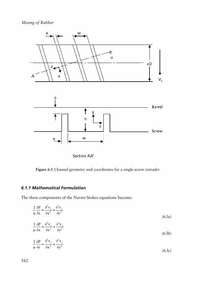
162

Mixing of Rubber

6.1.1 Mathematical Formulation

The three components of the Navier-Stokes equations become:

1�

�P�z

=�2vz

�x2+�2vz

�y2

(6.la)

1�

�P�x

=�2vx

�x2+�2vx

�y2

(6.lb)

1��P�y

=�2vy

�x2+�2vy

�y2

(6.lc)

Figure 6.1 Channel geometry and coordinates for a single-screw extruder

163

Continuous Mixers

and

�2vz

�x2<<

�2vz

�y2

(6.2)

because of the wide channel. The boundary conditions are:

vz(O,y) = 0 (6.3a)

vz{x,O) = 0 (6.3b)

vz (w,y) = 0 (6.3c)

vz (x,h) = V (6.3d)

where Vz is the downstream component of the barrel velocity relative to the screw. Using Equation (6.2), Equation (6.la) becomes:

1�

�P�z

=�2vz

�y2

(6. 4a)

vz(O) = 0 (6. 4b)

vz(x,h) = Vz (6.4c)

The solution to this equation is:

vz =

Vzyh

�y h� y( )

2��P�z

(6.5)

The volumetric throughput is calculated by:

Q = w vz y( )dy

0

h

� (6.6)

Substituting from Equation (6.5) yields:

Q =

Vzwh2

�wh2 �P / �z( )

12� (6.7)

The drag velocity component of the barrel with respect to the screw in the cross-channel direction Vx causes circulation in the channel which improves mixing. Equations (6.1b-c) and (6.2) combine to become:

1�

�P�x

=�2vx

�y2

(6.8)

164

Mixing of Rubber

with boundary conditions:

vx(0) = 0 (6.9a)

vx(h) = Vx (6.9b)

with a solution:

vx =

�yVx

h�

y h� y( )2�

�P�x

(6.10)

By assuming no leakage fl ow over the fl ight tips, the net fl ow in the cross-channel becomes:

vx y( )dy = 0

0

h

� (6.11)

Substituting Equation (6.10) and solving:

�P�x

=6�Vx

h (6.12)

and

vx =

yVx

h2

3yh

�

��

�

��

(6.13)

The relative barrel velocities are given by:

Vz = �DNcos* (6.l4a)

Vx = �DNsin* (6.14b)

where D is the barrel diameter, N is the screw speed and * is the screw pitch. The combined circulation fl ow cross-channel and drag fl ow down channel means that each fl uid element of the fl uid follows a helical trajectory. Following the analysis of Mohr, Saxton and Jepson [4], the amount of shear received by a fl uid element can be calculated. The shear in the cross-channel direction can be approximated by allowing an element to cross the entire width at one height h1 and then to return immediately at its complementary height h2 (Figure 6.2) given by:

vxdH = �

0

H1

� vxdHH2

1

� (6.15)

where the distance normal to the barrel surface has been made non-dimensional:

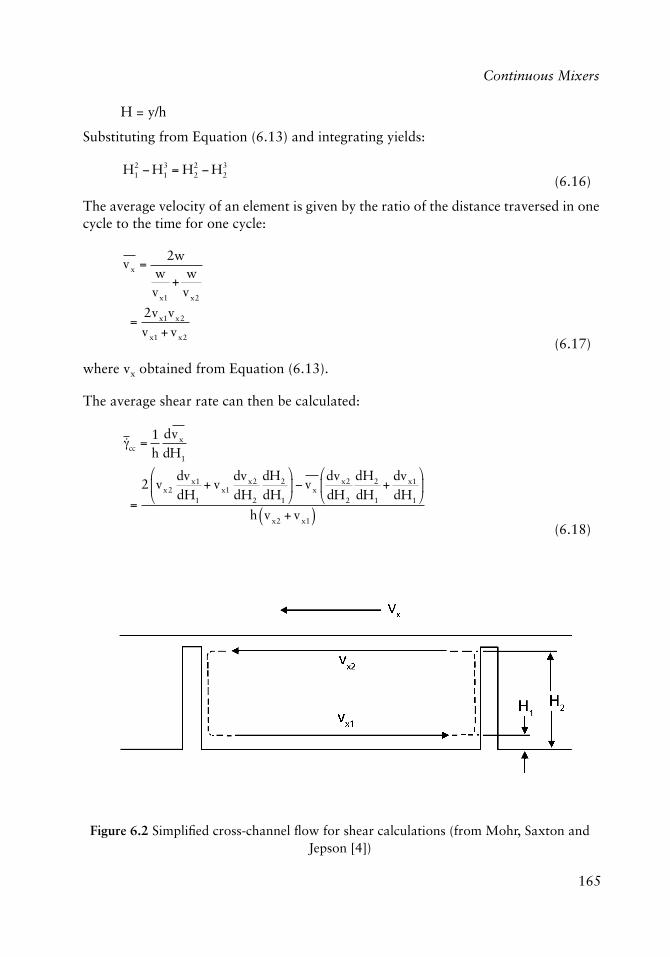
165

Continuous Mixers

H = y/h

Substituting from Equation (6.13) and integrating yields:

H12 H1

3 = H22 H2

3

(6.16)

The average velocity of an element is given by the ratio of the distance traversed in one cycle to the time for one cycle:

vx =2w

wvx1

+w

vx2

=2vx1vx2

vx1 + vx2 (6.17)

where vx obtained from Equation (6.13).

The average shear rate can then be calculated:

��cc =1h

dvx

dH1

=

2 vx2

dvx1

dH1

+ vx1

dvx2

dH2

dH2

dH1

�

��

�

� vx

dvx2

dH2

dH2

dH1

+dvx1

dH1

�

��

�

�

h vx2 + vx1( ) (6.18)

Figure 6.2 Simplifi ed cross-channel fl ow for shear calculations (from Mohr, Saxton and Jepson [4])

166

Mixing of Rubber

The average residence time in the channel for an element at H1 in a screw with length L is:

t =

L

vz1 sin� (6.19)

where vz1 is given below in Equation (6.25), and the total cross-channel shear is given by:

�cc =

1h

dvx

dH1

L

vz1 sin� (6.20)

Substituting:

a =

h2

6vz�

dPdz

(6.21)

into Equation (6.5) and using:

Vx

Vz

tan�

(6.22)

Equation (6.20) becomes:

�cc =L

h 1 a( ) cos�

dvx1

dH1

1

Vx

vz1

Vz

�

��

�

��a = 0

�

�

��

�

�

��

(6.23a)

=L

h 1 a( ) cos�Fc

(6.23b)

where:

Fc =dvx1dH1

1

Vx

vz1

Vz

�

��

�

��a = 0

(6.24)

and Fc depends only on H1 as tabulated in Table 6.1. As a, the ratio of pressure to drag fl ow, increases, the cross-channel shear In a similar manner, the average downstream velocity of a fl uid element initially at height H1 can be calculated:

167

Continuous Mixers

vz1 =

vz1

wvx1

�

��

�

��+ vz2

wvx2

�

��

�

��

wvx1

+wvx2

=vz1vx2 + vz2vx1

vx2 + vx1 (6.25)

where vz and vx correspond to heights H1 and H2. The average downstream shear rate can be calculated by differentiating with respect to H1 and substituting for the residence time yields the total shear downstream:

�DC =1h

dvz1

dH1

L

vz1 sin�

=L

hsin�FD

(6.26)

where FD is a dimensionless function of H1 (Table 6.1) given by:

FD =dv1

dH1

1

v1

�

��

�

��a = 0

=

vx2 + H1

dvx2

dH2

dH2

dH+ vx1

dH2

dH1

+ H2

dvx1

dH1

�

��

�

��

H1vx2 + H2vx1

+

v1

Vz

�

��

�

��

a=0

dvx2

dH2

dH2

dH1

+dvx1

dH1

�

��

�

��

H1vx2 + H2vx1 (6.27)

The shear components calculated in Equations (6.20) and (6.26) can be resolved into components parallel and perpendicular to the screw axis:

�D = �DC sin� �cc cos�

=Lh

FD Fc

1 a

�

��

�

��

(6.28a)

for the component parallel to the axis and:

�C = �DC cos� �cc sin�

=Lh

FD

tan�+

Fc tan�

1 a

�

��

�

��

(6.28b)

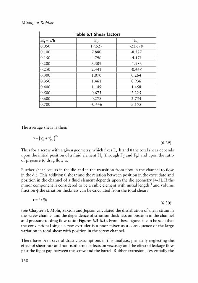
168

Mixing of Rubber

The average shear is then:

� = �cc

2 + �DC2( )1/2

(6.29)

Thus for a screw with a given geometry, which fi xes L, h and * the total shear depends upon the initial position of a fl uid element H1 (through FC and FD) and upon the ratio of pressure to drag fl ow a.

Further shear occurs in the die and in the transition from fl ow in the channel to fl ow in the die. This additional shear and the relation between position in the extrudate and position in the channel of a fl uid element depends upon the die geometry [4-5]. If the minor component is considered to be a cubic element with initial length l and volume fraction �,the striation thickness can be calculated from the total shear:

r = � / ��

(6.30)

(see Chapter 3). Mohr, Saxton and Jepson calculated the distribution of shear strain in the screw channel and the dependence of striation thickness on position in the channel and pressure-to-drag fl ow ratio (Figures 6.3-6.5). From these fi gures it can be seen that the conventional single screw extruder is a poor mixer as a consequence of the large variation in total shear with position in the screw channel.

There have been several drastic assumptions in this analysis, primarily neglecting the effect of shear rate and non-isothermal effects on viscosity and the effect of leakage fl ow past the fl ight gap between the screw and the barrel. Rubber extrusion is essentially the

Table 6.1 Shear factorsH1 = y/h FD FC

0.050 17.527 -21.678

0.100 7.880 -8.527

0.150 4.796 -4.171

0.200 3.309 -1.983

0.250 2.441 -0.648

0.300 1.870 0.264

0.350 1.461 0.936

0.400 1.149 1.458

0.500 0.675 2.225

0.600 0.278 2.754

0.700 -0.446 3.155

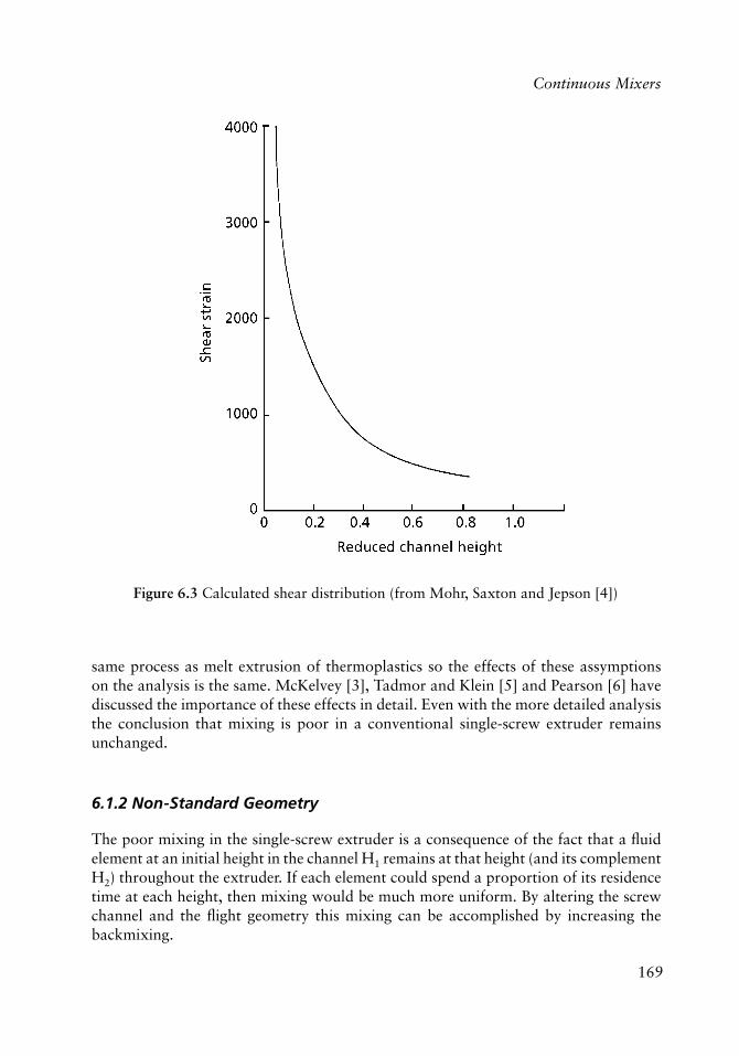
169

Continuous Mixers

same process as melt extrusion of thermoplastics so the effects of these assymptions on the analysis is the same. McKelvey [3], Tadmor and Klein [5] and Pearson [6] have discussed the importance of these effects in detail. Even with the more detailed analysis the conclusion that mixing is poor in a conventional single-screw extruder remains unchanged.

6.1.2 Non-Standard Geometry

The poor mixing in the single-screw extruder is a consequence of the fact that a fl uid element at an initial height in the channel H1 remains at that height (and its complement H2) throughout the extruder. If each element could spend a proportion of its residence time at each height, then mixing would be much more uniform. By altering the screw channel and the fl ight geometry this mixing can be accomplished by increasing the backmixing.

Figure 6.3 Calculated shear distribution (from Mohr, Saxton and Jepson [4])

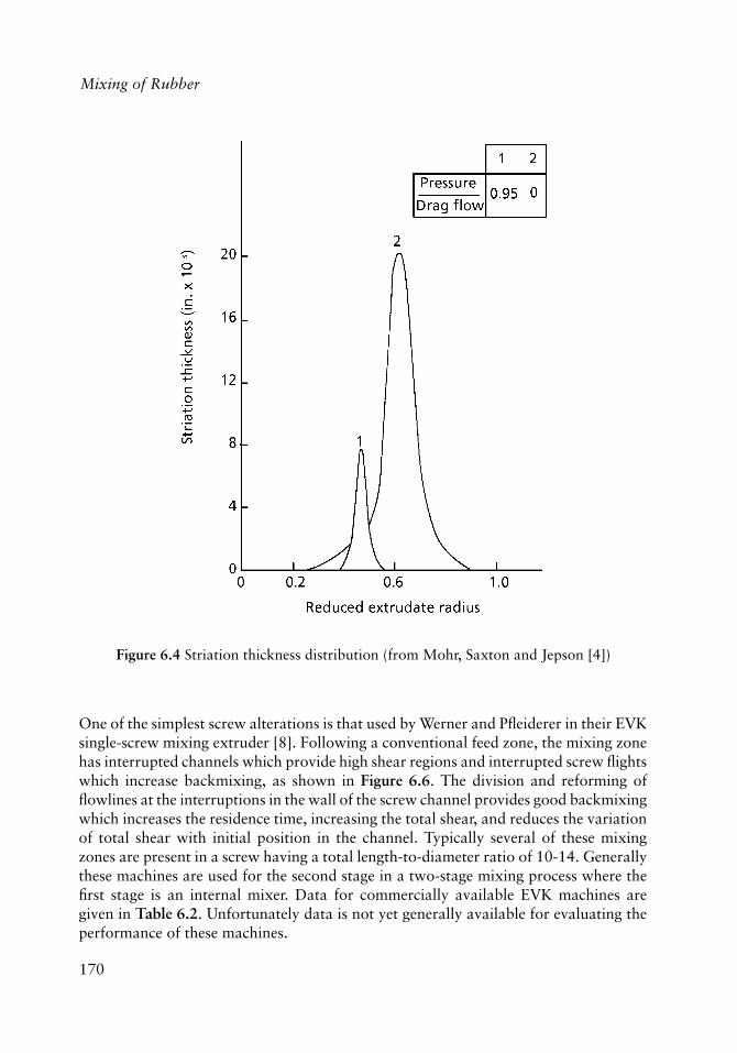
170

Mixing of Rubber

One of the simplest screw alterations is that used by Werner and Pfl eiderer in their EVK single-screw mixing extruder [8]. Following a conventional feed zone, the mixing zone has interrupted channels which provide high shear regions and interrupted screw fl ights which increase backmixing, as shown in Figure 6.6. The division and reforming of fl owlines at the interruptions in the wall of the screw channel provides good backmixing which increases the residence time, increasing the total shear, and reduces the variation of total shear with initial position in the channel. Typically several of these mixing zones are present in a screw having a total length-to-diameter ratio of 10-14. Generally these machines are used for the second stage in a two-stage mixing process where the fi rst stage is an internal mixer. Data for commercially available EVK machines are given in Table 6.2. Unfortunately data is not yet generally available for evaluating the performance of these machines.

Figure 6.4 Striation thickness distribution (from Mohr, Saxton and Jepson [4])

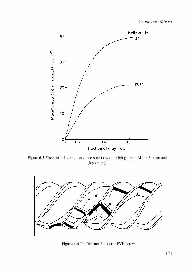
171

Continuous Mixers

Figure 6.5 Effect of helix angle and pressure fl ow on mixing (from Mohr, Saxton and Jepson [4])

Figure 6.6 The Werner-Pfl eiderer EVK screw

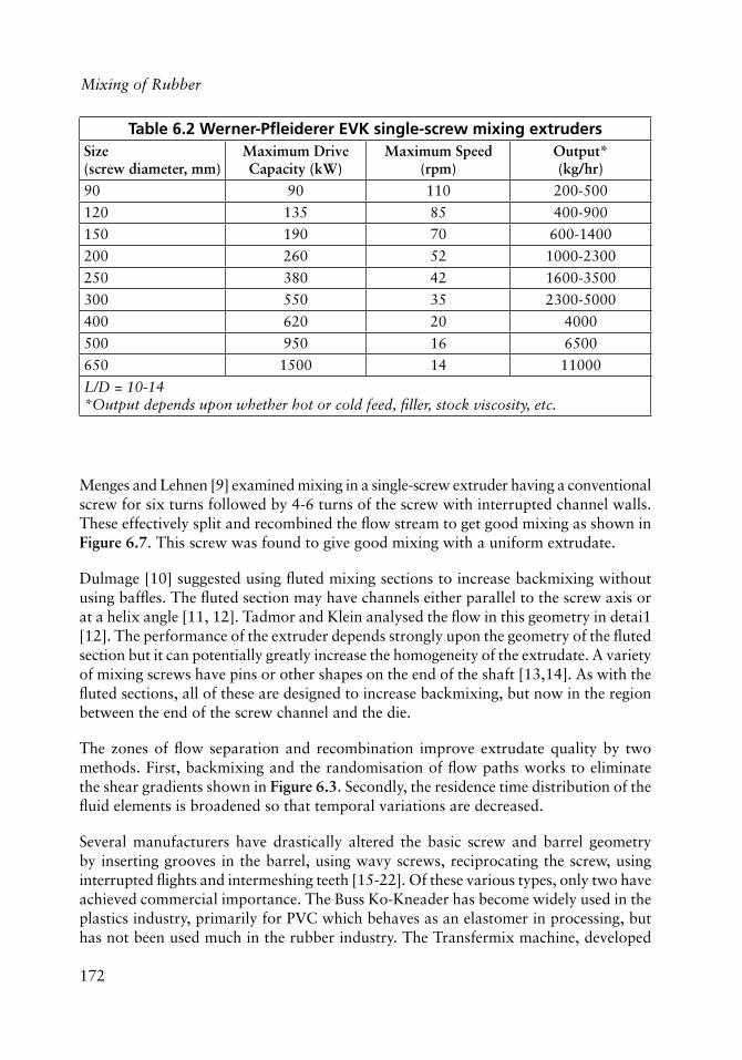
172

Mixing of Rubber

Menges and Lehnen [9] examined mixing in a single-screw extruder having a conventional screw for six turns followed by 4-6 turns of the screw with interrupted channel walls. These effectively split and recombined the fl ow stream to get good mixing as shown in Figure 6.7. This screw was found to give good mixing with a uniform extrudate.

Dulmage [10] suggested using fl uted mixing sections to increase backmixing without using baffl es. The fl uted section may have channels either parallel to the screw axis or at a helix angle [11, 12]. Tadmor and Klein analysed the fl ow in this geometry in detai1 [12]. The performance of the extruder depends strongly upon the geometry of the fl uted section but it can potentially greatly increase the homogeneity of the extrudate. A variety of mixing screws have pins or other shapes on the end of the shaft [13,14]. As with the fl uted sections, all of these are designed to increase backmixing, but now in the region between the end of the screw channel and the die.

The zones of fl ow separation and recombination improve extrudate quality by two methods. First, backmixing and the randomisation of fl ow paths works to eliminate the shear gradients shown in Figure 6.3. Secondly, the residence time distribution of the fl uid elements is broadened so that temporal variations are decreased.

Several manufacturers have drastically altered the basic screw and barrel geometry by inserting grooves in the barrel, using wavy screws, reciprocating the screw, using interrupted fl ights and intermeshing teeth [15-22]. Of these various types, only two have achieved commercial importance. The Buss Ko-Kneader has become widely used in the plastics industry, primarily for PVC which behaves as an elastomer in processing, but has not been used much in the rubber industry. The Transfermix machine, developed

Table 6.2 Werner-Pfl eiderer EVK single-screw mixing extrudersSize (screw diameter, mm)

Maximum Drive Capacity (kW)

Maximum Speed (rpm)

Output* (kg/hr)

90 90 110 200-500

120 135 85 400-900

150 190 70 600-1400

200 260 52 1000-2300

250 380 42 1600-3500

300 550 35 2300-5000

400 620 20 4000

500 950 16 6500

650 1500 14 11000

L/D = 10-14*Output depends upon whether hot or cold feed, fi ller, stock viscosity, etc.

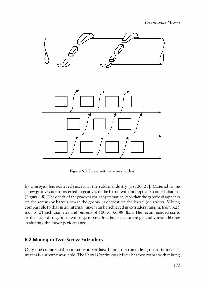
173

Continuous Mixers

Figure 6.7 Screw with stream dividers

by Uniroyal, has achieved success in the rubber industry [18, 20, 23]. Material in the screw grooves are transferred to grooves in the barrel with an opposite handed channel (Figure 6.8). The depth of the grooves varies systematically so that the groove disappears on the screw (or barrel) where the groove is deepest on the barrel (or screw). Mixing comparable to that in an internal mixer can be achieved in extruders ranging from 3.25 inch to 21 inch diameter and outputs of 600 to 35,000 lb/h. The recommended use is as the second stage in a two-stage mixing line but no data are generally available for evaluating the mixer performance.

6.2 Mixing in Two-Screw Extruders

Only one commercial continuous mixer based upon the rotor design used in internal mixers is currently available. The Farrel Continuous Mixer has two rotors with mixing

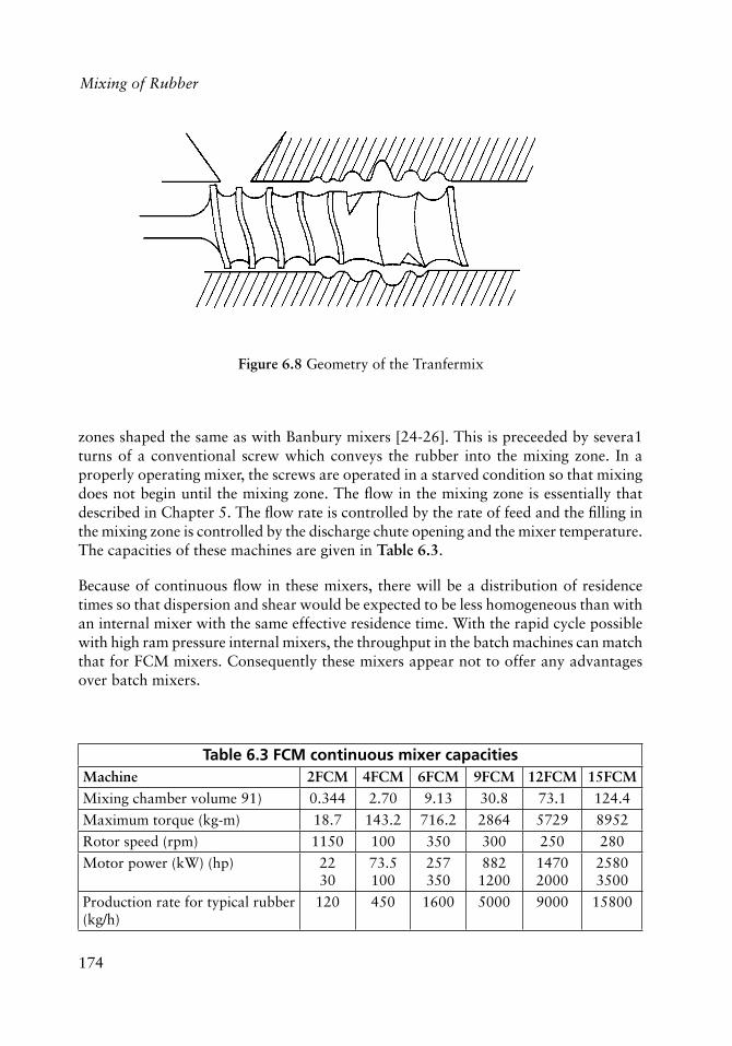
174

Mixing of Rubber

zones shaped the same as with Banbury mixers [24-26]. This is preceeded by severa1 turns of a conventional screw which conveys the rubber into the mixing zone. In a properly operating mixer, the screws are operated in a starved condition so that mixing does not begin until the mixing zone. The fl ow in the mixing zone is essentially that described in Chapter 5. The fl ow rate is controlled by the rate of feed and the fi lling in the mixing zone is controlled by the discharge chute opening and the mixer temperature. The capacities of these machines are given in Table 6.3.

Because of continuous fl ow in these mixers, there will be a distribution of residence times so that dispersion and shear would be expected to be less homogeneous than with an internal mixer with the same effective residence time. With the rapid cycle possible with high ram pressure internal mixers, the throughput in the batch machines can match that for FCM mixers. Consequently these mixers appear not to offer any advantages over batch mixers.

Figure 6.8 Geometry of the Tranfermix

Table 6.3 FCM continuous mixer capacitiesMachine 2FCM 4FCM 6FCM 9FCM 12FCM 15FCMMixing chamber volume 91) 0.344 2.70 9.13 30.8 73.1 124.4

Maximum torque (kg-m) 18.7 143.2 716.2 2864 5729 8952

Rotor speed (rpm) 1150 100 350 300 250 280

Motor power (kW) (hp) 2230

73.5100

257350

8821200

14702000

25803500

Production rate for typical rubber (kg/h)

120 450 1600 5000 9000 15800

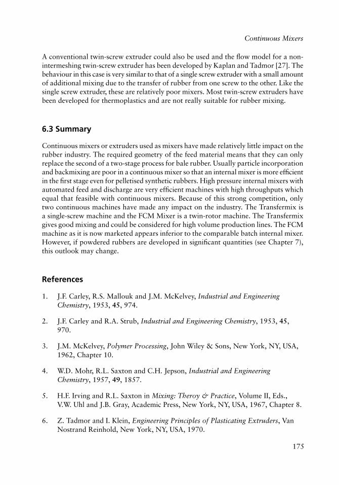
175

Continuous Mixers

A conventional twin-screw extruder could also be used and the fl ow model for a non-intermeshing twin-screw extruder has been developed by Kaplan and Tadmor [27]. The behaviour in this case is very similar to that of a single screw extruder with a small amount of additional mixing due to the transfer of rubber from one screw to the other. Like the single screw extruder, these are relatively poor mixers. Most twin-screw extruders have been developed for thermoplastics and are not really suitable for rubber mixing.

6.3 Summary

Continuous mixers or extruders used as mixers have made relatively little impact on the rubber industry. The required geometry of the feed material means that they can only replace the second of a two-stage process for bale rubber. Usually particle incorporation and backmixing are poor in a continuous mixer so that an internal mixer is more effi cient in the fi rst stage even for pelletised synthetic rubbers. High pressure internal mixers with automated feed and discharge are very effi cient machines with high throughputs which equal that feasible with continuous mixers. Because of this strong competition, only two continuous machines have made any impact on the industry. The Transfermix is a single-screw machine and the FCM Mixer is a twin-rotor machine. The Transfermix gives good mixing and could be considered for high volume production lines. The FCM machine as it is now marketed appears inferior to the comparable batch internal mixer. However, if powdered rubbers are developed in signifi cant quantities (see Chapter 7), this outlook may change.

References

1. J.F. Carley, R.S. Mallouk and J.M. McKelvey, Industrial and Engineering Chemistry, 1953, 45, 974.

2. J.F. Carley and R.A. Strub, Industrial and Engineering Chemistry, 1953, 45, 970.

3. J.M. McKelvey, Polymer Processing, John Wiley & Sons, New York, NY, USA, 1962, Chapter 10.

4. W.D. Mohr, R.L. Saxton and C.H. Jepson, Industrial and Engineering Chemistry, 1957, 49, 1857.

5. H.F. Irving and R.L. Saxton in Mixing: Theroy & Practice, Volume II, Eds., V.W. Uhl and J.B. Gray, Academic Press, New York, NY, USA, 1967, Chapter 8.

6. Z. Tadmor and I. Klein, Engineering Principles of Plasticating Extruders, Van Nostrand Reinhold, New York, NY, USA, 1970.

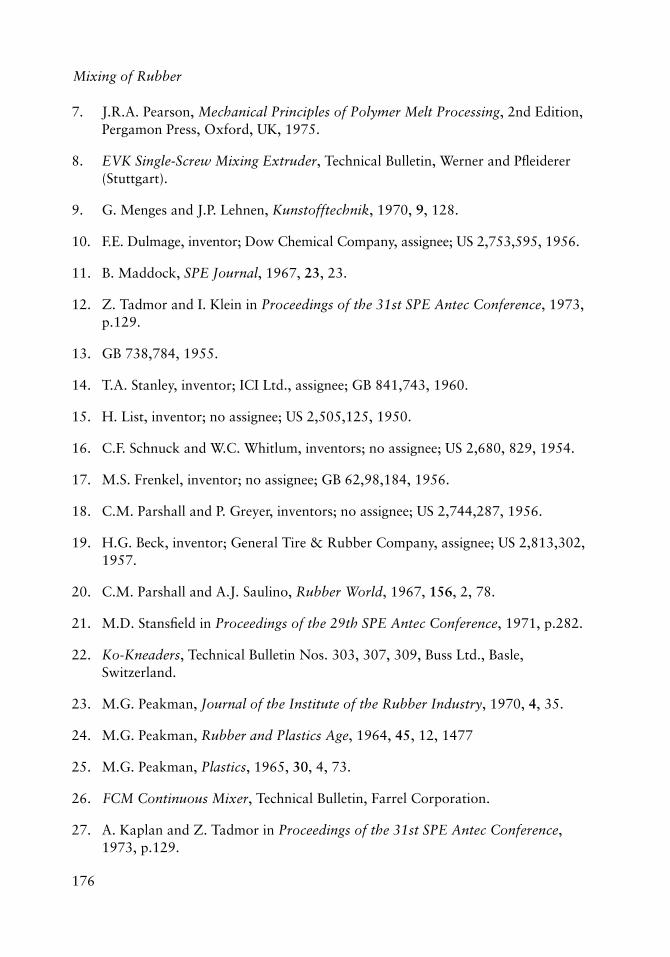
176

Mixing of Rubber

7. J.R.A. Pearson, Mechanical Principles of Polymer Melt Processing, 2nd Edition, Pergamon Press, Oxford, UK, 1975.

8. EVK Single-Screw Mixing Extruder, Technical Bulletin, Werner and Pfl eiderer (Stuttgart).

9. G. Menges and J.P. Lehnen, Kunstofftechnik, 1970, 9, 128.

10. F.E. Dulmage, inventor; Dow Chemical Company, assignee; US 2,753,595, 1956.

11. B. Maddock, SPE Journal, 1967, 23, 23.

12. Z. Tadmor and I. Klein in Proceedings of the 31st SPE Antec Conference, 1973, p.129.

13. GB 738,784, 1955.

14. T.A. Stanley, inventor; ICI Ltd., assignee; GB 841,743, 1960.

15. H. List, inventor; no assignee; US 2,505,125, 1950.

16. C.F. Schnuck and W.C. Whitlum, inventors; no assignee; US 2,680, 829, 1954.

17. M.S. Frenkel, inventor; no assignee; GB 62,98,184, 1956.

18. C.M. Parshall and P. Greyer, inventors; no assignee; US 2,744,287, 1956.

19. H.G. Beck, inventor; General Tire & Rubber Company, assignee; US 2,813,302, 1957.

20. C.M. Parshall and A.J. Saulino, Rubber World, 1967, 156, 2, 78.

21. M.D. Stansfi eld in Proceedings of the 29th SPE Antec Conference, 1971, p.282.

22. Ko-Kneaders, Technical Bulletin Nos. 303, 307, 309, Buss Ltd., Basle, Switzerland.

23. M.G. Peakman, Journal of the Institute of the Rubber Industry, 1970, 4, 35.

24. M.G. Peakman, Rubber and Plastics Age, 1964, 45, 12, 1477

25. M.G. Peakman, Plastics, 1965, 30, 4, 73.

26. FCM Continuous Mixer, Technical Bulletin, Farrel Corporation.

27. A. Kaplan and Z. Tadmor in Proceedings of the 31st SPE Antec Conference, 1973, p.129.

177

Powdered Rubbers

Powdered Rubbers

AuthorAuthor

Powdered rubbers have periodically generated great interest in the past ten years, primarily based on the efforts with BF Goodrich in the USA and its European affi liates. The possible advantages of powdered rubbers will be presented in this chapter.

7.1 Preparation

To date the only commercially available powdered rubber is an acrylonitrile-butadiene rubber (NBR) manufactured by BF Goodrich. Powdered rubbers have a particle size less than 1 mm diameter which distinguishes them from conventional pellets or granules for use in the common extrusion line. Because of their small unit size, powders have a relatively large surface-to-volume ratio. Three methods have been described for the preparation of powders from emulsion rubbers, although the same processes could be used for natural rubber latex [1].

7.1.1 Mechanical Pulverisation (Grinding)

Conventional shredders produce too large a particle (2-20 mm) so high impact pulverisers are used. Large amounts of air are needed to remove the frictional heat. As an alternative, the rubber may be cooled below its glass transition temperature with liquid nitrogen and then pulverised. The main disadvantage of this method is the energy costs.

7.1.2 Spray Drying

The emulsion is forced through a nozzle countercurrent to a stream of hot air which dries the particles before they coalesce. The main disadvantage of this process is that the emulsifi ers will be incorporated into the product and this may adversely affect vulcanisation rate and other compound properties.

7

178

Mixing of Rubber

7.1.3 Coagulation

By proper selection of electrolytes, a fi nely divided powder can be formed. This can be coagulated with large amounts of carbon black as a masterbatch or treated with small amounts of antimassing agents such as zinc oxide or zinc stearate. The wet powder is dried on a vacuum fi lter followed by a fl uidised bed.

Each of these methods require additional raw materials handling and energy expenditure which sets a price premium on the cost to the rubber processor. This has been one of the major obstacles to acceptance of powdered rubbers in the industry despite the offsetting advantages of this material.

7.2 Mixing Powdered Rubbers

Initially the fi llers and additives such as carbon black and the rubber are intimately mixed, as in blending (Chapter 2), before phase coalescence occurs and the rubber forms a continuous matrix. In this regime, simple mixing occurs rapidly with little shear mixing. When coalescence occurs, fi ller particles are already well distributed throughout the bulk of the material so the only energy required is that to reduce the carbon black agglomerate particle size and to move the particles small distances, on the length scale of the initial rubber particle size. Less shear is required for this process than is required for slab rubber, where large shears are required to distribute the material uniformly through the rubber. The stock temperature is signifi cantly lower in the powdered rubber so that the viscosity, hence the shear stress, is higher and particle breakup is more readily achieved. Another advantage of the lower temperature is that often vulcanising ingredients can be added with the carbon black in a one-stage process rather than two stages.

Wardle and Sercombe [2] pre-blended the powdered nitrile rubber, carbon black and vulcanising agents in a T.K. Felder Turbo Rapid Mixer such as is used in PVC technology [3] The dry ingredients were added at the beginning of the cycle and mixed 2 minutes at 800 rpm and 1 minute at 2000 rpm. Speed was reduced to 800 rpm for the addition of liquid ingredients then increased to 2000 rpm for 1 minute. The total mixing time in the blender was 5 minutes and the product was a free-fl owing powder with a maximum temperature of 60-65 °C, which means low scorch. The powder was then sheeted and mixed an additional nine minutes on a conventional 6 inch two-roll mill. The mill capacity was 300-350 kg/h compared to 70 kg/h for slab rubber mixed on the same mill.

A more useful comparison is powdered rubber versus bale rubber in an internal mixer [4]. Bale rubber, pre-mixed powdered rubber and unmixed powdered nitrile rubber were mixed in a small Banbury mixer at 77 rpm and with cooled rotors. It was found that powdered rubbers had a higher power peak than bale rubbers. The mixing was complete in one stage with the powdered rubbers but bale rubbers required 25-60% more energy in a second stage to reach the same degree of carbon dispersion. Consequently, the mixing

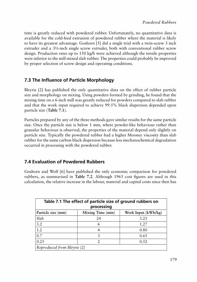
179

Powdered Rubbers

time is greatly reduced with powdered rubber. Unfortunately, no quantitative data is available for the cold-feed extrusion of powdered rubber where the material is likely to have its greatest advantage. Goshorn [5] did a single trial with a twin-screw 3 inch extruder and a 3½-inch single screw extruder, both with conventional rubber screw design. Production rates up to 150 kg/h were achieved although the tensile properties were inferior to the mill-mixed slab rubber. The properties could probably be improved by proper selection of screw design and operating conditions.

7.3 The Infl uence of Particle Morphology

Bleyrie [2] has published the only quantitative data on the effect of rubber particle size and morphology on mixing. Using powders formed by grinding, he found that the mixing time on a 6-inch mill was greatly reduced for powders compared to slab rubber and that the work input required to achieve 99.5% black dispersion depended upon particle size (Table 7.1).

Particles prepared by any of the three methods gave similar results for the same particle size. Once the particle size is below 1 mm, where powder-like behaviour rather than granular behaviour is observed, the properties of the material depend only slightly on particle size. Typically the powdered rubber had a higher Mooney viscosity than slab rubber for the same carbon black dispersion because less mechanochemical degradation occurred in processing with the powdered rubber.

7.4 Evaluation of Powdered Rubbers

Goshorn and Wolf [6] have published the only economic comparison for powdered rubbers, as summarised in Table 7.2. Although 1965 cost fi gures are used in this calculation, the relative increase in the labour, material and capital costs since then has

Table 7.1 The effect of particle size of ground rubbers on processing

Particle size (mm) Mixing Time (min) Work Input (kWh/kg)Slab 24 3.23

3.2 6 1.27

1.2 4 0.80

0.7 3 0.65

0.25 2 0.52

Reproduced from Bleyrie [2]

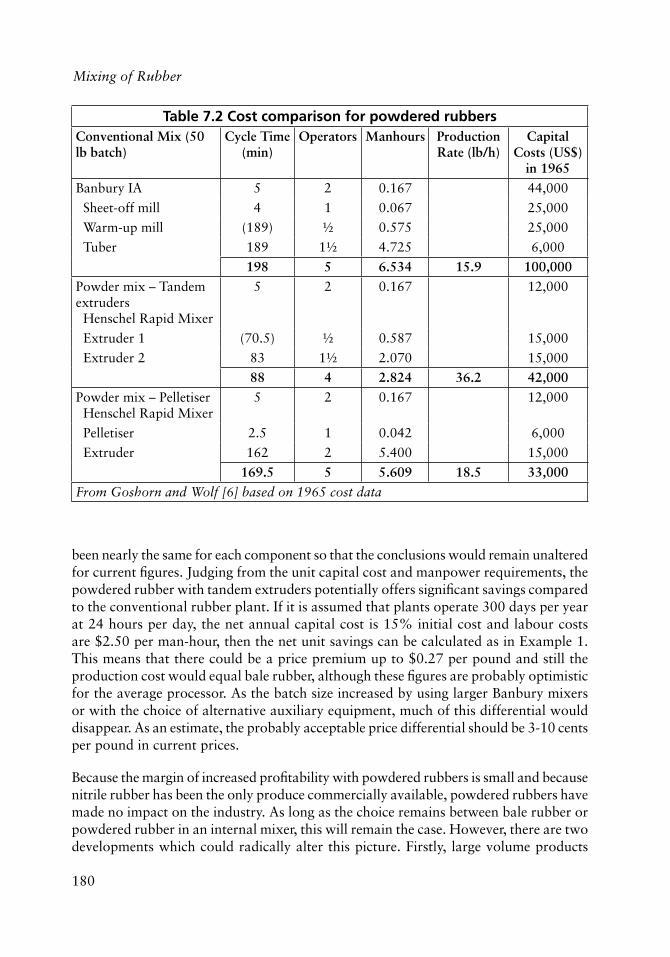
180

Mixing of Rubber

been nearly the same for each component so that the conclusions would remain unaltered for current fi gures. Judging from the unit capital cost and manpower requirements, the powdered rubber with tandem extruders potentially offers signifi cant savings compared to the conventional rubber plant. If it is assumed that plants operate 300 days per year at 24 hours per day, the net annual capital cost is 15% initial cost and labour costs are $2.50 per man-hour, then the net unit savings can be calculated as in Example 1. This means that there could be a price premium up to $0.27 per pound and still the production cost would equal bale rubber, although these fi gures are probably optimistic for the average processor. As the batch size increased by using larger Banbury mixers or with the choice of alternative auxiliary equipment, much of this differential would disappear. As an estimate, the probably acceptable price differential should be 3-10 cents per pound in current prices.

Because the margin of increased profi tability with powdered rubbers is small and because nitrile rubber has been the only produce commercially available, powdered rubbers have made no impact on the industry. As long as the choice remains between bale rubber or powdered rubber in an internal mixer, this will remain the case. However, there are two developments which could radically alter this picture. Firstly, large volume products

Table 7.2 Cost comparison for powdered rubbersConventional Mix (50 lb batch)

Cycle Time (min)

Operators Manhours Production Rate (lb/h)

Capital Costs (US$)

in 1965Banbury IA 5 2 0.167 44,000

Sheet-off mill 4 1 0.067 25,000

Warm-up mill (189) ½ 0.575 25,000

Tuber 189 1½ 4.725 6,000

198 5 6.534 15.9 100,000Powder mix – Tandem extruders Henschel Rapid Mixer

5 2 0.167 12,000

Extruder 1 (70.5) ½ 0.587 15,000

Extruder 2 83 1½ 2.070 15,000

88 4 2.824 36.2 42,000Powder mix – Pelletiser Henschel Rapid Mixer

5 2 0.167 12,000

Pelletiser 2.5 1 0.042 6,000

Extruder 162 2 5.400 15,000

169.5 5 5.609 18.5 33,000From Goshorn and Wolf [6] based on 1965 cost data

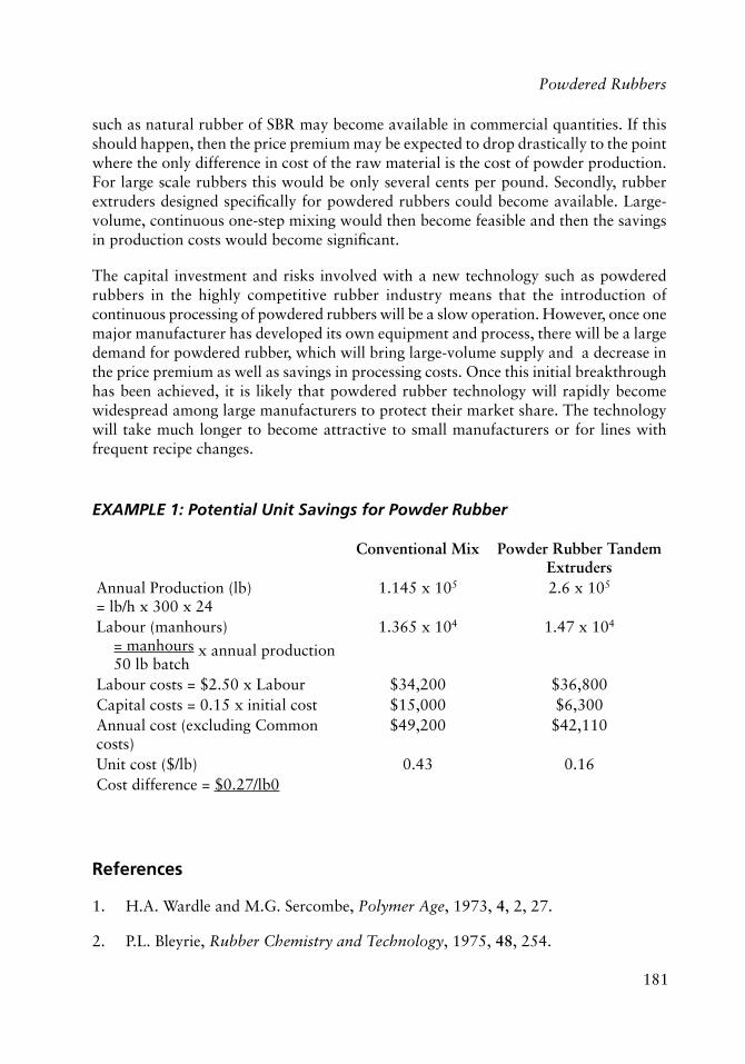
181

Powdered Rubbers

such as natural rubber of SBR may become available in commercial quantities. If this should happen, then the price premium may be expected to drop drastically to the point where the only difference in cost of the raw material is the cost of powder production. For large scale rubbers this would be only several cents per pound. Secondly, rubber extruders designed specifi cally for powdered rubbers could become available. Large-volume, continuous one-step mixing would then become feasible and then the savings in production costs would become signifi cant.

The capital investment and risks involved with a new technology such as powdered rubbers in the highly competitive rubber industry means that the introduction of continuous processing of powdered rubbers will be a slow operation. However, once one major manufacturer has developed its own equipment and process, there will be a large demand for powdered rubber, which will bring large-volume supply and a decrease in the price premium as well as savings in processing costs. Once this initial breakthrough has been achieved, it is likely that powdered rubber technology will rapidly become widespread among large manufacturers to protect their market share. The technology will take much longer to become attractive to small manufacturers or for lines with frequent recipe changes.

EXAMPLE 1: Potential Unit Savings for Powder Rubber

Conventional Mix Powder Rubber Tandem Extruders

Annual Production (lb)= lb/h x 300 x 24

1.145 x 105 2.6 x 105

Labour (manhours) = manhours 50 lb batch

1.365 x 104 1.47 x 104

Labour costs = $2.50 x Labour $34,200 $36,800Capital costs = 0.15 x initial cost $15,000 $6,300Annual cost (excluding Common costs)

$49,200 $42,110

Unit cost ($/lb) 0.43 0.16Cost difference = $0.27/lb0

x annual production

References

1. H.A. Wardle and M.G. Sercombe, Polymer Age, 1973, 4, 2, 27.

2. P.L. Bleyrie, Rubber Chemistry and Technology, 1975, 48, 254.

182

Mixing of Rubber

3. Turbo Rapid Mixers, Technical Bulletin, T.K. Felder Ltd., Eastleigh, UK.

4. W.H. Whittington and M.E. Woods, European Rubber Journal, 1975, 157, 9, 24.

5. T.R. Goshorn, Journal of the Institution of the Rubber Industry, 1972, 6, 2, 77.

6. T.R. Goshorn and F.R. Wolf, Rubber Age, 1965, 97, 8, 77.

183

Index

AAcrylonitrile-butadiene rubber 177

BBack-mixing 12, 169-170, 172, 175Blender, drum 32Blenders, pneumatic 41Blending efficiency 16, 22, 24Blending, particle 43Blending ratios calculation 15Brabender mixer 61Brabender mixing curve 109

CCartesian coordinate system 45, 53, 71, 112Coagulation 178Cold-feed extrusion 179Commercial internal mixers 134Confidence limits 9-10

confidence limits for the mean 9confidence limits for the variance 10

Confidence of the mean test 12Confidence of the variance test 13

DDeborah number 94, 102, 103, 105, 155-156, 158Dibutyl phosphate absorption test 65

GGardner pre-mixer 36Gaussian distribution 8, 18Graetz number 98, 103, 156-158Griffiths number 98, 103-104, 156-158Guth-Gold equation 65

184

Mixing of Rubber

HHoppers, meter-blending 40

MMarkov chain 24-26, 41Markov process 25, 27Masterbatches 62-64Maxwell fluid 94Mechanical pulverisation 177Mill, capacities of 104Mixedness 15-16, 18Mixer, Banbury 63, 89, 133, 140, 147, 152, 153, 174, 178Mixer, Banbury 11d 119Mixer, Battaggion ribbon 3Mixer, Bolen and Colwell model 126Mixer, continuous 2, 161, 175Mixer, dispersive 43, 52, 61, 113, 116Mixer, Farrel continuous 173Mixer, Farrel-Bridge Banbury 134-135Mixer, FCM 174-175Mixer, Francis-Shaw intermix 134Mixer. fluidised 38Mixer, gravity feed 36Mixer, internal 2, 43, 63, 69, 100, 103, 107, 108, 112, 124-126, 131, 133, 137-138,

154-155, 161, 173-174, 180Mixer, Pari 36Mixer, pneumatic 40Mixer, Winkworth ribbon blade 35Mixer, rapid batch 37Mixing cycle 131Mixing, degree of 16-18, 20-21, 29, 31, 40, 45, 60Mixing equipment 30

tumble blender 30-33, 41blade mixers 30, 33air mixers 30, 36

Mixing, kinetics of simple 18Mixing, laminar 1, 50Mixing, laminar shear 43, 51, 64, 67, 88, 161Mixing time, constant 153Mixing, in single screw extruders 161Mixing, in twin screw extruders 173Mixing process 27, 29, 40, 67, 70, 137Mixing, of powdered rubbers 178Mixing, simple 5-6, 20, 24, 43, 51, 110Mixing time 89, 99, 100-101, 103, 107, 119, 133, 146, 154, 158

185

Index

Mixing, scale of 45Mill, two-roll rubber 69Mill, two-roll 2, 78, 107Morphology, particle 179Mohr’s analysis 121Mooney viscosity 67, 95, 148, 151-152, 158Multicomponent mixtures 24

NNatural rubber 181Navier-Stokes equations 162Newtonian fluid 53-54, 56, 70-71, 76, 82, 84, 86, 96, 98, 100-102, 105, 115-116,

142-143Newtonian liquid 58Newtonian viscosity 97Null hypothesis test 10

PPoisson distribution 8, 18Polybutadiene milling 95Powdered rubber 177-178, 180-181Power-law fluid 80, 87, 119-120, 142, 150

RRam pressure 131-132Ribbon blender blades 33-34, 40-41

Gardner interrupted spiral agitator 34Winkworth ribbon blade 34-35Winkworth contra-flow blade 34

Rubber, bale 178, 180Rubber extrusion 168Rubber industry 1, 65, 69, 172, 175, 181Rubber matrix 43, 48, 50, 52, 63, 65, 67, 109-110Rubber mill 93, 137Rubber, milling of 69Rubber, mill-mixed slab 179Rubber mixing 1, 3, 44

SScale-up process 101Scaling laws 84, 121, 137Scaling rules 139Schematic Brabender mixing curve 109Shaw intermix 136, 141Shear stress, maximum 142-144

186

Mixing of Rubber

Significance tests 10significance of the mean test (Student’s t-test) 10, 14

significance of the variance (F-test) 11significance of the distribution ( 2 –test) 11, 14

Silicone rubbers 69Single screw extruder 162, 169, 172, 175, 179Sisind meter blender 39Spray drying 177Student’s t-test 9Stupachenko model 126Symmetric mill 76-77, 82Synthetic rubber 89

TTemperature, constant stock 154Total shear strain 145, 148, 154-155, 158Trough blender 33Tumbler blender geometry 31Tumble blending, kinetics of 23Tumbler mixers, kinetics of 19

VViscoelastic Model 123Vulcanisation 1

WWeissenberg number 93, 95, 102-103, 155-156, 158Werner and Pfleiderer internal mixers GKN 134, 137, 142Werner-Pfleiderer EVK screw 171Werner-Pfleiderer EVK single-screw mixing extruders 172

Shawbury, Shrewsbury, Shropshire, SY4 4NR, UK Telephone: +44 (0)1939 250383 Fax: +44 (0)1939 251118 Web: www.rapra.net

Published by Smithers Rapra, 2009

Since the discovery of vulcanisation in the nineteenth century, rubber has

been a major industrial product. From its inception, the use of vulcanising

agents, reinforcing fillers and other additives has been a major feature of the

rubber industry. Innumerable articles and texts attest to the chemist’s skill in

balancing the chemical and physical properties of the manufactured prod-

ucts.

In most cases, experimenters have been concerned with how recipe changes

affect the product properties while the physical processes which formed the

test specimen are not considered. For the rubber processor, however, it is

these mechanical operations which form the heart of his business. Despite

the commercial importance of the mixing process, no comprehensive analysis

of rubber mixing, considered as a unit operation, is currently available. This

monograph is designed to fill that gap in the arsenal available for problem

solving by the production engineer or the machine designer.

This book is a reprint of a book originally published in the 1970s and has

been republished due to the interest that there still is for this type of infor-

mation about rubber mixing.

It will be of interest to all those who are involved in the manufacture of rub-

ber goods and to those who are studying the subject.

ISBN: 978-1-84735-151-7

Documents

Mixing Of Rubber - ccsuniversity.ac.in · Mixing as a general operation may be considered as three basic processes occurring simultaneously. Simple mixing ensures that the mixture