Embed Size (px)
Citation preview
*The corresponding authors: Robert K. Prud’homme: Email [email protected]
Phone (609) 258-4577 Fax (609) 258-0211 Rodney O. Fox: Email rofox iastate.edu Phone (515) 294-9104 Fax (515) 294-2689
Mixing in a Multi-Inlet Vortex Mixer (MIVM) for Flash NanoPrecipitation
Ying Liu1, Chungyin Cheng2, Ying Liu2, Robert K. Prud’homme1*and Rodney O. Fox2 *
1 Department of Chemical Engineering, Princeton University
2 Department of Chemical and Biological Engineering, Iowa State University
Abstract
Rapid precipitation of both organic and inorganic compounds at high supersaturation
requires homogenous mixing to control the particle size distribution. We present the
design and characterization of a new Multi-Inlet Vortex Mixer (MIVM). The four-stream
MIVM allows control of both the supersaturation and the final solvent quality by varying
stream velocities. The design also enables the separation of reactive components prior to
mixing. Finally, the design enables mixing of streams of unequal volumetric flows, which
is not possible with alternate confined impinging jet (CIJ) mixing geometries. We
characterize the mixing performance of the MIVM using competitive fast reactions (the
so called “Bourne reactions”). Adequate micromixing is obtained with a suitably defined
Reynolds number when Re > 1600. The experimental results are compared to CFD
simulations of the fluid mechanics and parallel reactions in the MIVM. Excellent
correspondence is found between the simulation and the experimental results with no
adjustable parameters. The CFD simulations provide a powerful tool for the optimization
of these complex mixing geometries.
2
Keywords: mixing, Multi-Inlet Vortex Mixer (MIVM), Nanoprecipitation,
Computational Fluid Dynamics (CFD), Reynolds number, competitive reactions.
Introduction
The production of uniform-sized nanoparticles of hydrophobic organic compounds by an
economical, scalable process is a considerable challenge. It is motivated by the use and
potential use of nanoparticles in drug delivery, especially poorly water soluble drugs1-4,
cosmetics 5-7, dyes 3, 8, medical imaging and diagnostic9, 10, and pesticides 11. One of the
advanced processes to produce nanoparticles is “Flash NanoPrecipitation”12, which
requires fast mixing of two or more streams to create supersaturation. A dissolved solute
and stabilizing amphiphilic polymer are rapidly mixed with an anti-solvent to create high
supersaturation over a time scale shorter than the characteristic nucleation and growth
time scales for the nanoparticles. This rapid growth from a uniform concentration field
and uniform “poisoning” of the nanoparticle surfaces by adsorbed amphiphilic polymer
uniformly stops the growth to produce narrow particle size distributions. The process can
also provide the capability to coat particles and create composite multi-functional
particles.
An understanding of rapid precipitations requires an understanding of the role of
macro-, meso- and micromixing on the development of supersaturation. Various mixing
devices have been proposed and characterized, including semibatch stirred-tank
precipitators 13 and impinging-jet precipitators 14. In a previous study, Johnson and
Prud’homme determined the dependence of mixing time on Reynolds number and
geometry in a Confined Impinging Jet (CIJ) mixer using the conversion of competitive

3
reactions (the so called “Bourne reactions”) 15. Mixing in the CIJ can be as fast as
milliseconds, but the CIJ mixer is limited by the requirement of equal momenta of the
solvent and anti-solvent streams. The final concentration of the effluent is the average of
the two stream concentrations which may compromise particle stability.
To overcome the limitation of the CIJ mixer, but to retain its ability to provide rapid
micromixing, scalability, and ease of operation, we developed a Multi-Inlet Vortex Mixer
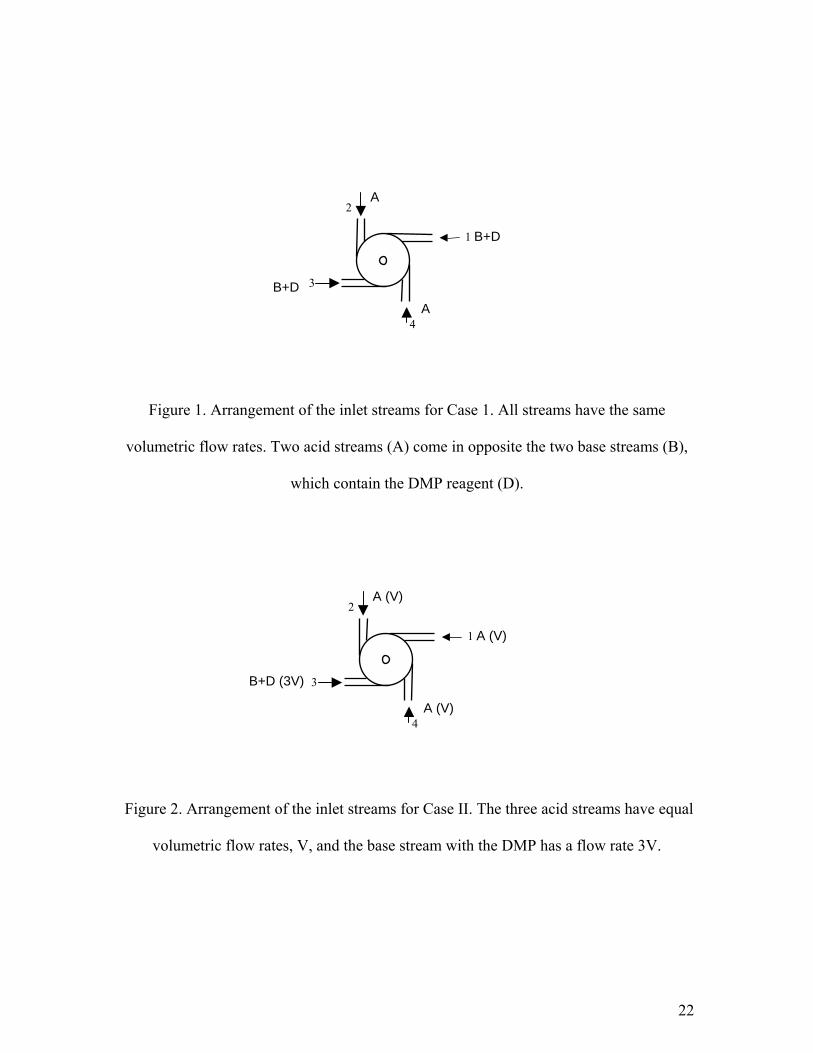
(MIVM) (Fig. 1). The concept of the MIVM is that the momentum from each stream
contributes independently to drive micromixing in the cell. Therefore, it is possible to
have one or more streams at high volumetric flow rate and another steam at a lower flow
rate and still get good micromixing. The design question is -- how efficiently will the
mixer operate at different flow velocities and stream ratios? How does it compare to the
CIJ where two opposing streams impinge and all the momentum is dissipated in the
central region of the cavity? If the MIVM provides rapid micromixing then it has the
operational advantages that the final fluid phase is predominantly anti-solvent. This
increases the stability of the nanoparticles by depressing the rate of Ostwald ripening 16-
19. In addition, being able to separate inlet streams enables the introduction of reactive
compounds in different streams so that reactive precipitations can be accomplished.
In this paper, we establish the functionality of the mixing time of this MIVM with
Reynolds number, inlet velocity, physical properties of the streams and the geometry of
the mixer. The characteristic mixing time of the MIVM is measured by the competitive
Bourne reactions.15, 20-23 The characteristic mixing time of the MIVM can be in the range
of milliseconds at Re > 1600. A CFD model that was previously used to model the CIJ
4
mixer was used to model the MIVM mixer.24 The CFD results provide additional insights
as to the mixing mechanisms in the MIVM mixer.
Reaction kinetics
Baldyga, Bourne, and Walker20, 22 developed a competitive reaction scheme that is fast
enough to probe the mixing performance of mixing in the MIVM. This “fourth Bourne
reaction” has stable reactants and products, and is easily quantified by gas
chromatography (GC). Conceptually, the scheme works in this way. The reagents for the
competitive reactions are segregated in two (or more) flow streams. If the micromixing is
faster than the reaction kinetics of the slow reaction then the conversion of the limiting
reagent in the slow reaction will correspond to the ratio of the two reaction rate constants;
that is, the conversion can be calculated from the conversion from a homogeneous initial
state. However, if the reacting streams are not well mixed, then diffusion limitations will
decrease the conversion of the limiting reagent.15
The fast reaction of the competitive reactions is the neutralization of sodium
hydroxide with a second-order rate constant 8 31 1.4 10 m /mol s= × ⋅k ,
2OH H H O− ++ → .
The slow reaction is the acid catalyzed hydrolysis of 2,2-dimethoxypropane (DMP) to
form one mole of acetone and two moles of methanol,
3 3 2 3 2 3 3 3CH C(OCH ) CH H ( H O) CH COCH 2CH OH H+ ++ + → + + . .
The rate constant of this reaction is 32 0.63m /mol s= ⋅k .

5
Since the rate constant of the fast reaction is more than 108 times the rate constant of
the slow reaction, the reaction time can be expressed as a pseudo first-order time constant
of the slow reaction:
2 0
1τ =rxnDMPk C
, (1)
where 0DMPC is the DMP concentration after mixing but before the reaction. The mixing
effectiveness is measured by the fraction of DMP reacted,
0
1= − DMP
DMP
NXN
, (2)
where DMPN and 0DMPN are the molar flow rate of DMP after and before the reaction,
respectively. For the experiments, Eqn. 2 was cast in the form,
,
,
112
⎛ ⎞= +⎜ ⎟⎝ ⎠
MeOH outlet
DMP inlet
CX
C F, (3)
where F is the flow ratio of the DMP and NaOH streams/HCl streams. ,MeOH outletC is the
methanol concentration at the outlet of the MIVM, which can be accurately measured by
GC, and ,DMP inletC is the DMP concentration before mixing at the inlet of the MIVM. The
constant “2” in front of CDMP,inlet comes from the fact that every mole of DMP that reacts
will generate two moles of methanol.
Conceptually, mixing can be described by a mixture fraction ξ 25, which is
independent of chemistry. By convention, we will set 0ξ = in the streams containing acid,
and 1ξ = in the streams containing base and DMP. The value of the average mixture
fraction at the outlet is,

6
2
1 2
ξ =+m
m m, (4)
where m2 is the summation of the mass flow rate of the streams containing DMP, and m1
is the summation of the mass flow rate of other streams. The fraction of DMP converted
can be evaluated numerically from,
,
,
1ξ
= − DMP outlet
DMP inlet
CX
C, (5)
where,
,1 2
1 ρ=+ ∫ iDMP outlet DMPC c U ndS
m m (6)
is the “mixing-cup” average at the outlet. Note if DMP were completely mixed at the
outlet (which is usually not the case) then ,DMP outletC would be equal to the outlet
concentration of DMP.
Experimental Section
Experiment apparatus
Digitally controlled syringe pumps (Harvard Apparatus, PHD 2000 programmable,
Holliston, MA) were used to provide constant and accurate flow rates for the inlet
streams of the MIVM. Gas chromatography (GC) HP 5890A (Hewlett Packard,
Wilmington, DE) with an autosampler (6890 series injector, Agilent Technologies, Palo
Alto, CA) was used to analyze the amount methanol generated compared with ethanol.
Samples preparation
7
Samples were prepared using MilliQ water. The molar ratio of HCl and NaOH is 1:1.05
to ensure that all the acid is consumed. The molar ratio of DMP and NaOH is 1:1 in
solution. In every acid or base and DMP solution, 25 vol% of ethanol and 90 mmol/L
NaCl were added to DI water. The ethanol serves as an internal GC standard, and the salt
suppresses ionic interactions in the reaction. DMP 99+ and 1.000 molar standard NaOH
and HCl were purchased from Aldrich.
Arrangement of Inlet Streams
Case I:
The arrangement of the inlet streams is symmetric as shown in Figure 1.
The streams have equal velocities. Two opposing streams are acid with initial
concentration 33.0 mole/m3, and the other two opposing streams are base and DMP
streams with base concentration 34.65 mole/m3 and DMP concentration 33.0 mole/m3.
The ratio of acid to base to DMP is 1:1.05:1. After homogenous mixing without reaction,
the DMP concentration would be 16.5 mole/m3, which gives a characteristic reaction time
is 96.2 ms.
Case II:
The arrangement of the inlet streams is shown in Figure 2. Three streams are acid streams
with the same velocity. The last stream is the base and DMP stream with velocity three
times that of the acid streams. The acid concentration in each of the acid streams is 33.0
mole/m3. Base concentration is 34.65 mole/m3, and DMP is 33.0 mole/m3. The
stoichiometry of the acid, base and DMP is 1:1.05:1. The reaction time is 96.2 ms (from
Eqn. 1).

8
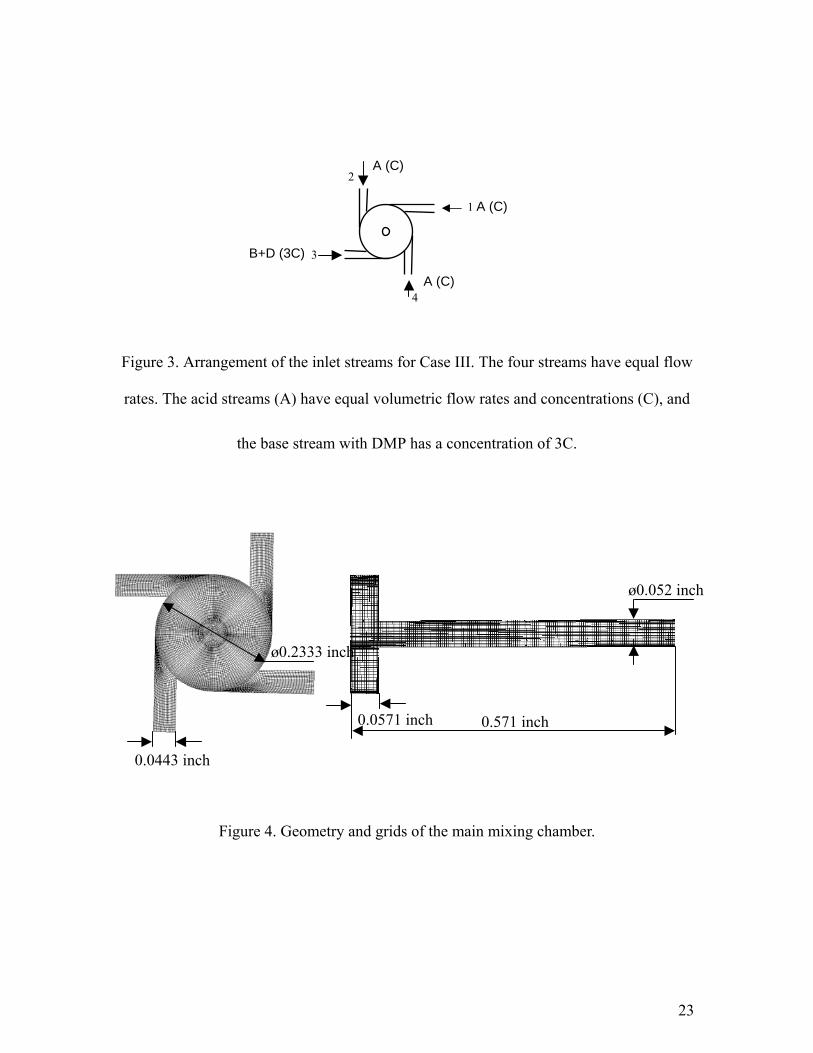
Case III:
The arrangement of the inlet streams is shown in Figure 3. All the streams have the same
velocity. Three of them are acid streams with concentration 22.0 mole/m3. The fourth
stream is base and DMP stream with base concentration 69.3 mole/m3and the DMP
concentration is 66.0 mole/m3. The ratio of acid, base and DMP, after homogenous
mixing before any reaction occurs, is 1:1.05:1, therefore the reaction time is 96.2 ms.
The definition of the Reynolds number (Re) is
1,
Re i
i N i
V Dν=
= ∑ , (7)
where iV is the velocity of nth inlet stream, D is the chamber diameter (D=0.2333 inch as
in Figure 1), iν is the kinematic viscosity of the nth inlet stream, and N is the number of
inlet streams.
Numerical Simulation
CFD model
In this work, we used the two-environment DQMOM-IEM model implemented by Liu
and Fox26. The transport equations for the mixture fraction ξn , and slow reaction progress
variable nY in the nth (n=1 or 2) environments are solved. The conserved scalars are
1p , 1 1ξp , 2 2ξp , 1 1p Y , 2 2p Y , and 2 11= −p p . 1p and 2p are the mass fraction of fluid
coming from the acid streams and the streams containing base and DMP, respectively.
Without showing the detailed derivation, the model equations are,
( ) ( )11 1
ρρ ρ
∂+∇ ⋅ = ∇⋅ Γ ∇
∂ T
pU p p
t (8)
9
( ) ( ) ( ) ( ) ( )2 21 11 1 1 1 1 2 2 1 1 1 2 2
1 2
ρ ξ ρρ ξ ρ ξ ργ ξ ξ ξ ξξ ξ
∂ Γ+∇⋅ = ∇ ⋅ Γ ∇ + − + ∇ + ∇⎡ ⎤⎣ ⎦∂ −
TT
pU p p p p p p
t (9)
( ) ( ) ( ) ( ) ( )2 22 22 2 2 2 1 2 1 2 1 1 2 2
2 1
ρ ξ ρρ ξ ρ ξ ργ ξ ξ ξ ξξ ξ
∂ Γ+∇⋅ =∇⋅ Γ ∇ + − + ∇ + ∇⎡ ⎤⎣ ⎦∂ −
TT
pU p p p p p p
t(10)
( ) ( ) ( ) ( )
( ) ( )
1 11 1 1 21 1 2 2 1
2 21 1 2 2 1 1 1
1 2
,
ρρ ρ ργ
ρ ρ ξ∞
∂+∇ ⋅ = ∇ ⋅ Γ ∇ + −⎡ ⎤⎣ ⎦∂
Γ+ ∇ + ∇ +
−
T
T
p YU p Y p Y p p Y Y
t
p Y p Y p S YY Y
(11)
( ) ( ) ( ) ( )
( ) ( )
2 22 2 2 2 1 2 1 2
2 21 1 2 2 2 2 2
2 1
,
ρρ ρ ργ
ρ ρ ξ∞
∂+∇ ⋅ = ∇ ⋅ Γ ∇ + −⎡ ⎤⎣ ⎦∂
Γ+ ∇ + ∇ +
−
T
T
p YU p Y p Y p p Y Y
t
p Y p Y p S YY Y
(12)
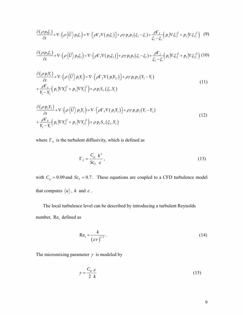
where TΓ is the turbulent diffusivity, which is defined as
2
TT
C kSc
µ
εΓ = , (13)
with 0.09Cµ = and 0.7TSc = . These equations are coupled to a CFD turbulence model
that computes u , k and ε .
The local turbulence level can be described by introducing a turbulent Reynolds
number, 1Re defined as
( )1 1/ 2Re kεν
= . (14)
The micromixing parameter γ is modeled by
2φ εγ =
Ck
(15)

10
with 2φ ≈C for high-Reynolds-number flow. It has been demonstrated by Liu and Fox
that at finite turbulent Reynolds numbers 2Cφ = overestimates the micromixing rate.
They propose the expression,26
( )6
10 1 10
lg Re for Re 0.2nn
nC aφ
=
= ≥∑ (16)
to account for finite Reynolds-number effects when the Schmitt number is large. Here,
0 1 2 3 4 5 60.4093, 0.6015, 0.5815, 0.09472, 0.3903, 0.1461 and 0.01604a a a a a a a= = = = = − = = − .
More detailed derivation can be found from Fox’s articles as well as others24-26.
With the assumption that the fast reaction was instantaneous, which implies that acid
and base cannot coexist at any point, the chemical reaction progress variable for the slow
reaction, Y , is determined by ξ through the chemical source term, S∞ , which is
( )2 2 0 2 2 11 2 2
, 1 if 0 and 0ss s s
S Y A k Y Yξ ξ ξξ ξ ξξ ξ ξ∞
⎛ ⎞⎛ ⎞= − − ≤ ≤ ≤ ≤⎜ ⎟⎜ ⎟
⎝ ⎠⎝ ⎠, (17)
where,
01
0 0
ξ =+sA
A B (18)
and
02
0 0
ξ =+sA
A D. (19)
0A , 0B and 0D are the inlet molar concentrations of the acid, base and DMP.
11
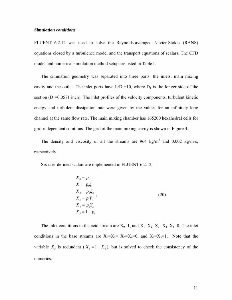
Simulation conditions
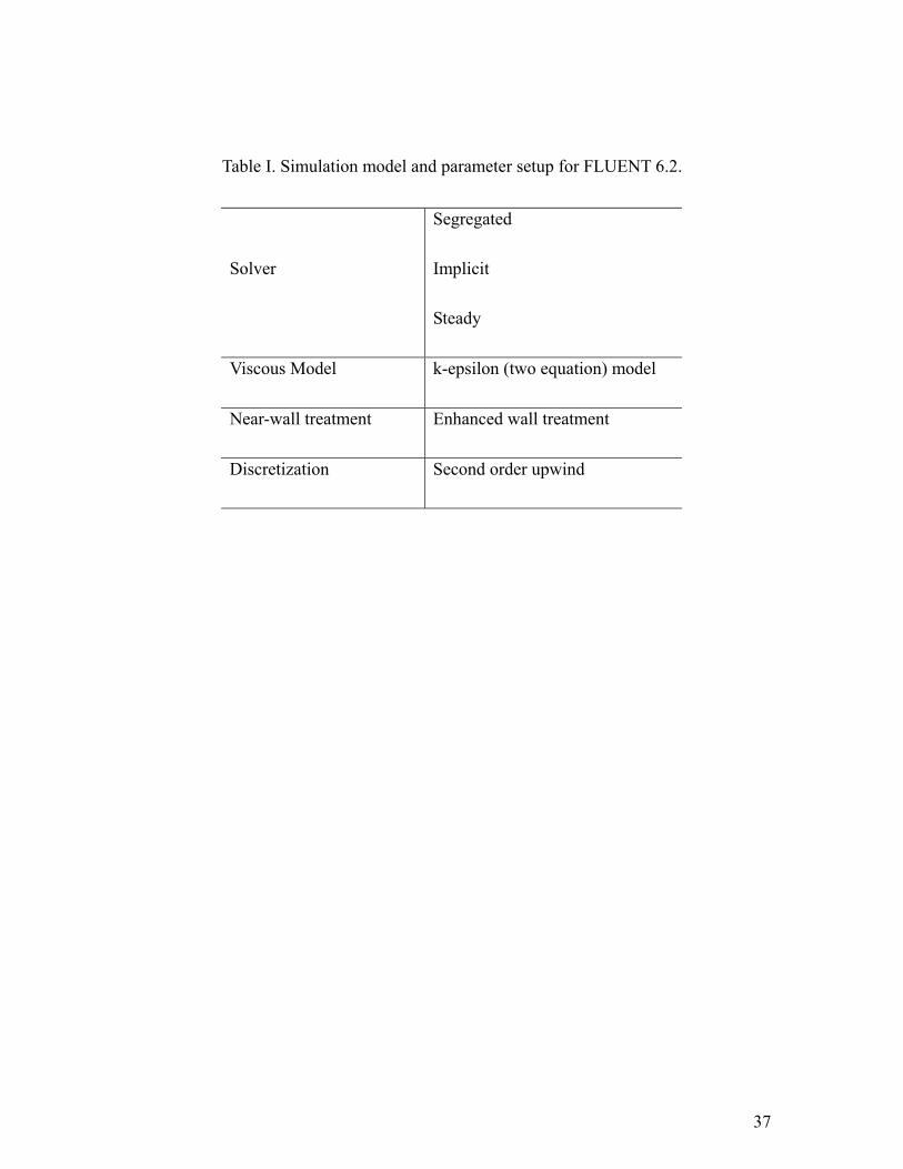
FLUENT 6.2.12 was used to solve the Reynolds-averaged Navier-Stokes (RANS)
equations closed by a turbulence model and the transport equations of scalars. The CFD
model and numerical simulation method setup are listed in Table I.
The simulation geometry was separated into three parts: the inlets, main mixing
cavity and the outlet. The inlet ports have L/D1=10, where D1 is the longer side of the
section (D1=0.0571 inch). The inlet profiles of the velocity components, turbulent kinetic
energy and turbulent dissipation rate were given by the values for an infinitely long
channel at the same flow rate. The main mixing chamber has 165200 hexahedral cells for
grid-independent solutions. The grid of the main mixing cavity is shown in Figure 4.
The density and viscosity of all the streams are 964 kg/m3 and 0.002 kg/m-s,
respectively.
Six user defined scalars are implemented in FLUENT 6.2.12,
0 1
1 1 1
2 2 2
3 1 1
4 2 2
5 11
X pX pX pX p YX p YX p
ξξ
====== −
, (20)
The inlet conditions in the acid stream are X0=1, and X1=X2=X3=X4=X5=0. The inlet
conditions in the base streams are X0=X1= X3=X4=0, and X2=X5=1. Note that the
variable 5X is redundant ( 5 01X X= − ), but is solved to check the consistency of the
numerics.

12
Results and discussion
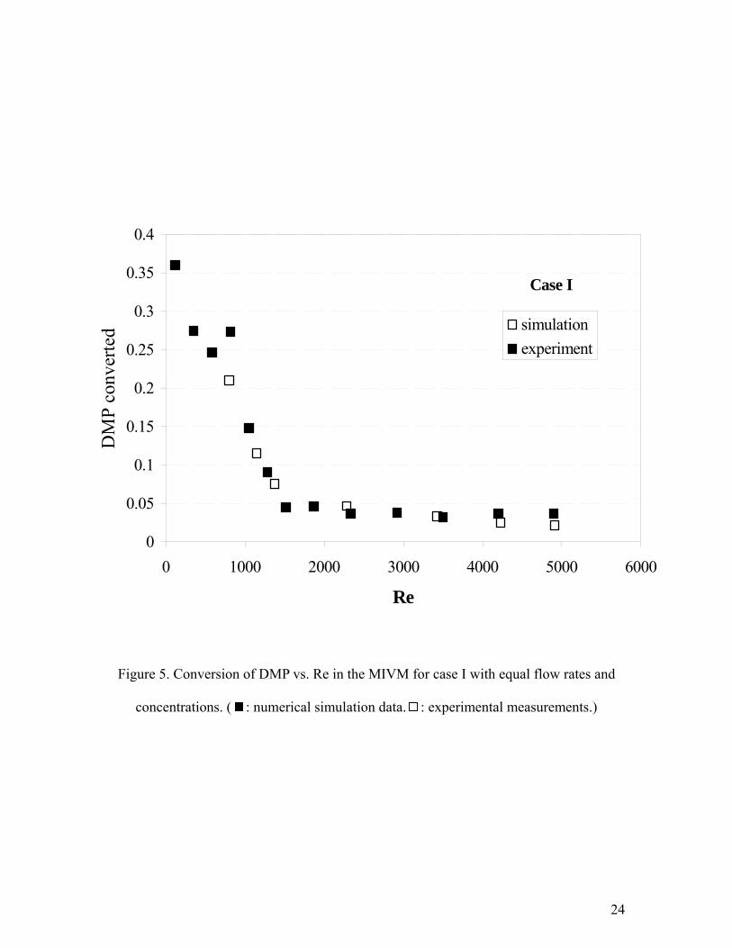
Case I:
The experimental and numerical simulation data for the DMP conversion versus
Reynolds number are reported in Fig. 5.
The simulation results and the experimental measurements are in close agreement in
the range 800 Re 5000≤ ≤ . At higher Re, experimental measurements reach a lower limit,
since DMP can be hydrolyzed in water solution even without the presence of acid.
The numerical simulation shows that when Re > 1600, essentially all of the mixing is
completed in the main mixing chamber, all the acid is consumed at the outlet of the main
mixing cavity, and DMP conversion ceases to increase. But with lower Re, reaction
continues in the outlet tube. Computational studies were conducted using an extended
outlet tube. Each time a tube with a length ten times of the outlet diameter was added at
the end and the solution was recomputed. This procedure was continued until the DMP
conversion was complete (i.e., acid was completely consumed).
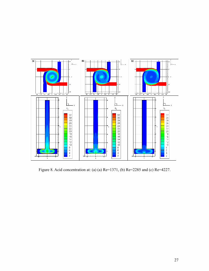
The mixing details of the points at Re=4227 (inlet velocity=0.37 m/s), Re=2285 (inlet
velocity=0.2 m/s) and Re=1371 (inlet velocity=0.12 m/s) are shown in Fig. 6. The highest
turbulent kinetic energy is near the outlet of the chamber for each case. But for low Re,
the very center of the chamber has a low kinetic energy. With increasing Re, the zone of
highest kinetic energy moves into the center of the chamber. This observation is in
contrast to our previous results for the CIJ mixer in which the kinetic energy dissipation
is maximum in the center of the mixing cavity24. As a result considerable mixing occurs
in the exit region of the MIVM.

13
From Figs. 7 and 8, it can be seen that with higher Re, the mixing volume increases;
compositional uniformity is achieved faster; and acid is consumed more quickly.
Case II:
The experimental and numerical simulation data of DMP conversion versus Reynolds
number are reported in Fig. 9. Once more we observe both experimentally and
numerically that at higher Re, the mixing was improved, and the turning point appears
near Re=1600.
Case III:
The experimental and numerical simulation data of the DMP conversion versus
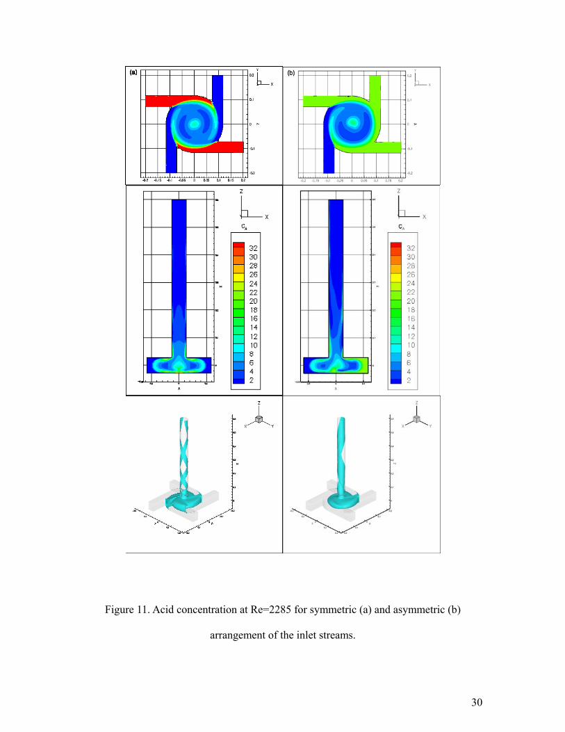
Reynolds number are reported in Fig. 10. A comparison of case I and case III shows that
at low Re the symmetric arrangement of the inlet streams results in somewhat better
mixing; that is the conversion of DMP is always lower for the symmetric arrangement.
Concentrating the reagents in a single stream (case III) results in somewhat worse mixing.
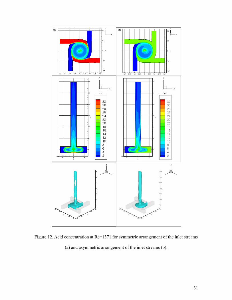
The 3-dimensional depiction of the acid concentration in Figs. 11 and 12 shed light on the
origin of the effect. In case I, Fig. 11a, the two acid streams swirl down the exit tube as
thin filaments. For case III, Fig. 11b, with the single concentrated acid stream the length
scale of acid segregation is obviously larger, and therefore mixing poorer. At the lower
Reynolds number (Fig. 12) the effect is even more pronounced.
Mixing Scales
At high Re, there is generally a separation of mixing scales. The large-scale motions
are mainly influenced by the geometry of the reactor, and the small-scale motions are
determined by energy dissipation rate and viscosity.
14
For the case of two types of inlet streams, the mixture-fraction mean, ξ , can be
written as
1 1 2 2p pξ ξ ξ= + , (21)
Likewise, the mixture-fraction variance, 2'ξ , can be written as
22 2 21 1 2 2' p pξ ξ ξ ξ= + − , (22)
Large-scale segregation (LSS) in the reactor can be described by introducing a LSS
variance,
( )22'LSS
ξ ξ ξ= − . (23)
where ξ is the average mixture fraction after complete mixing, which is equal to 0.5 in
our cases.
The LSS zone can be determined using 2 2'ξ σ>LSS
and 2 2'ξ σ< , where σ is the
cut-off standard deviation. The reactions are controlled by SSS alone if 2 2'ξ σ<LSS
and
2 2'ξ σ≥ . And in the condition that 2 2'LSS
ξ σ≥ and 2 2'ξ σ≥ , the reactions are
controlled by both LSS and SSS.
From the transport equations of 2'LSS
ξ reported by Ying Liu25, the characteristic
decay time for 2'LSS
ξ is given by,
2
2
'
2
ξ
ξ=
Γ ∇LSS
LSS
T
t . (24)
15
The characteristic decay time for SSS variance, also known as the micromixing time in
turbulent-mixing theory, is given by,
12γ
=SSSt . (25)
Then, the characteristic mixing time is obtained by
= +mix LSS SSSt t t . (26)
Considering case I (the case with one opposing pair of inlets containing acid and the
other containing base and DMP), extracting data at different heights of the reactor can
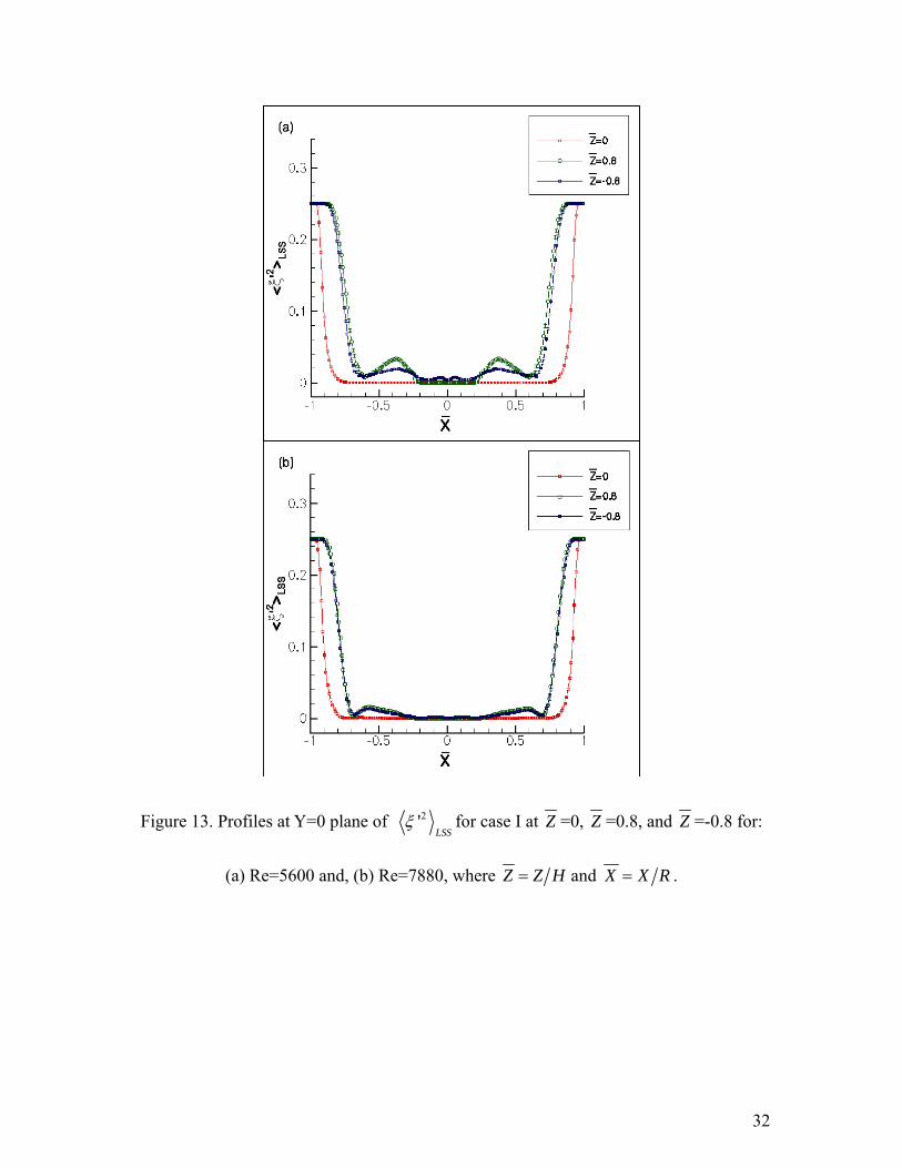
provide more detailed information about the change of 2'LSS
ξ and 2'ξ . The heights
are chosen to emphasize the changes in mixing variables. In the reactor chamber, ξ is
not equal to ξ , indicating the presence of LSS. As seen in Figure 13, 2'LSS
ξ decays
quickly after inlet streams enter the reactor. At 0Z = , where Z Z H= and H is the half
thickness of the reactor chamber, 2'LSS
ξ remains 0, indicating that mixing is mainly
affected by SSS in this zone. On the other hand, 2'LSS
ξ has slight variations at
0.8Z = − and 0.8Z = , indicating mixing is affected by LSS in these regions.
Considering the change of 2'ξ at 0Z = in Figure 14, the SSS mixture-fraction
variance is slightly lower at the edge area for the lower Re than higher Re; on the other
hand, it changes faster and is higher near the reactor center ( 0Z = ) for lower Re. The
same characteristics are also shown at 0.8Z = − , 2'ξ is much larger for lower Re than
higher Re. These differences arise when Re is small -- the flow motions are more

16
laminar-like and thus φC is smaller. The flow streams are mostly dominated by the
geometry of the reactor as they enter and swirl from periphery to the center, where the
velocity is the highest and therefore the change of mixture-fraction is greatest. Compared
to a low Re case, better mixing takes place at higher Re. Since the flow motions tend to
be more turbulent, the variation of mixture-fraction is not as great.
Segregation Zones
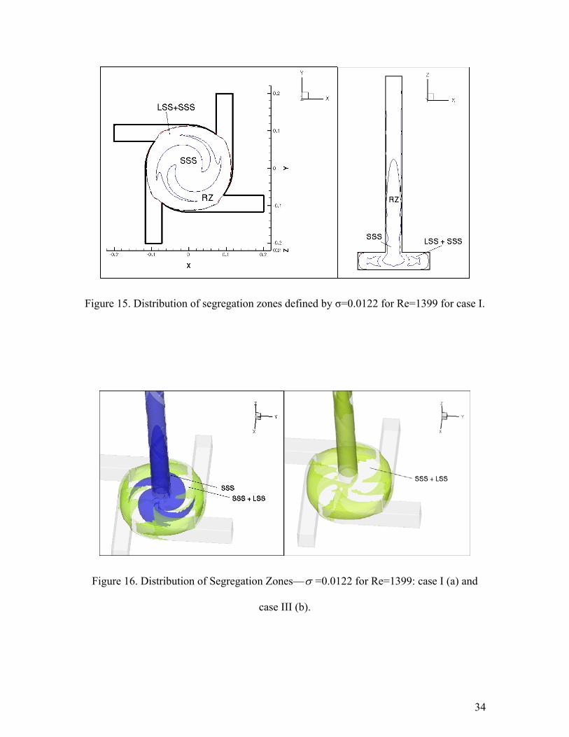
In case I, both LSS + SSS and SSS overlap with the reaction zone at the center planes as
shown in Figure 15, where the cut-off standard deviation was defined as the distance in
mixture-fraction space from the end of the reactions ( 1sξ ) to complete mixing (ξ ); i.e.,
0122.01 =−= sξξσ .
While in case I the reaction zone overlaps with both SSS and LSS+SSS zones, in case
III, 2'LSS
ξ decays much more slowly and only an LSS+SSS zone can be identified as
shown in Figure 16. These results show that in case III, mixing and reaction are
influenced mainly by the geometry of the MIV reactor, resulting in relatively poorer
mixing performance.
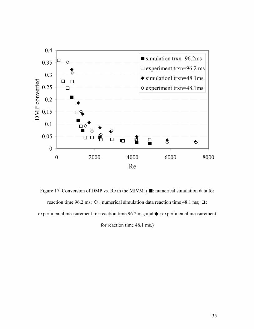
Reaction time
The reaction time is expressed as the pseudo first-order time constant of the slow
reaction, as in Eqn. 1. Therefore, the reaction time is dependent on the initial DMP
concentration.
The experimental and numerical simulation results with reaction time 48.1ms and
96.2ms are shown in Figure 17 for case I.
17
At high Re, for both reaction times, the conversion of DMP reaches the same limit,
which is set by the sensitivity of the competitive reactions. That is the mixing time is
faster than the reaction time and the compositions appear essentially homogeneous. For
both reaction times the agreement between the simulations and experimental data is good.
Four inlet streams vs. two inlet streams
The comparison of the MIVM with four inlet streams and two inlet streams by numerical
simulation is show in Figure 18.
The results show that at the same total volume flow rate, the MIVM with four inlet
streams has better mixing than the MIVM with the same geometry but two inlet streams.
The mixing difference can be attributed to the initially larger segregation length scales
with only two inlets. However, the differences in performance are not substantial.
Conclusion
The flexibility and capability of the MIVM for fast micromixing has been demonstrated.
The concept behind that MIVM is that each stream contributes independently to the
micromixing in the chamber. Both competitive reactions and CFD simulations show that
the mixer operates in essentially this way. Changes in the flow rate of individual streams,
or concentration of reactants in one stream rather than distribution between two streams
makes a relatively minor change in the performance of the MIVM. Another way of
saying this is that the choice of definition of the Reynolds number as a linear combination
of the stream velocities (Eqn. 7) seems to represent the mixing performance of the MIVM
over a relatively wide range of inlet conditions. Operation of the MIVM at Reynolds
number above 1600 ensures homogeneous mixing for reactions with time constants

18
longer than 50 ms. This insensitivity of the MIVM to inlet stream configuration makes it
a flexible and useful mixing device.
There are observable, second-order, differences between operations with different
inlet configurations. Four equal velocity streams with the reactants distributed
symmetrically between the four streams (case I) is more efficient than either unequal
stream velocities (case II) or equal stream velocities but unequal reactant distributions
(case III). Also, four symmetric streams is more efficient than two symmetric streams at
the same Reynolds number. The CFD simulations show that with two inlet streams the
length scales of segregation are larger, which results in somewhat inferior mixing.
The ability of the CFD to quantitatively predict mixing and fast competitive
reactions is quite striking. It demonstrates that the CFD simulations can be used to design
and optimize the design of mixing geometries with a high level of confidence.
Acknowledgments:
This work was supported financially by the U.S. National Science Foundation though the
NIRT “Nanoscale Interdisciplinary Research Teams” (CTS-0506966) awarded to
Princeton University, University of Minnesota, and Iowa State University.
Reference:
1. Muller, R. H.; Peters, K., Nanosuspensions for the formulation of poorly soluble
drugs - I. Preparation by a size-reduction technique. International Journal of
Pharmaceutics 1998, 160, (2), 229-237.

19
2. Kipp, J. E., The role of solid nanoparticle technology in the parenteral delivery of
poorly water-soluble drugs. International Journal of Pharmaceutics 2004, 284, (1-2),
109-122.
3. Horn, D.; Rieger, J., Organic nanoparticles in aqueous phase. Angew. Chem. Int.
Ed. 2001, 40, 4330-4361.
4. Allemann, E.; Gurny, R.; Doelker, E., Drug-loaded nanoparticles - Preparation
methods and drug targeting issues. European Journal of Pharmaceutics and
Biopharmaceutics 1993, 39, (5), 173-191.
5. Muller, R. H.; Radtke, M.; Wissing, S. A., Solid lipid nanoparticles (SLN) and
nanostructured lipid carriers (NLC) in cosmetic and dermatological preparations.
Advanced Drug Delivery Reviews 2002, 54, S131-S155.
6. Zhao, Q. Q.; Boxman, A.; Chowdhry, U., Nanotechnology in the chemical
industry-opportunities and challenges. Journal of Nanoparticle Research 2003, 5, 567-
572.
7. Crandall, B. C.; Lewis, J., Nanotechnology: Research and perspectives.
Cambridge: MIT press., 1992; p 251-267.
8. Gesquiere, A. J.; Uwada, T.; Asahi, T.; Masuhara, H.; Barbara, P. F., Single
molecule spectroscopy of organic dye nanoparticles. Nano Letters 2005, 5, (7), 1321-
1325.
9. Romanus, E.; Huckel, M.; Gross, C.; Prass, S.; Weitschies, W.; Brauer, R.; Weber,
P., Magnetic nanoparticle relaxation measurement as a novel tool for in vivo diagnostics.
Journal Of Magnetism And Magnetic Materials 2002, 252, (1-3), 387-389.

20
10. Riviere, C.; Boudghene, F. P.; Gazeau, F.; Roger, J.; Pons, J. N.; Laissy, J. P.;
Allaire, E.; Michel, J. B.; Letourneur, D.; Deux, J. F., Iron oxide nanoparticle-labeled rat
smooth muscle cells: Cardiac MR imaging for cell graft monitoring and quantitation.
Radiology 2005, 235, (3), 959-967.
11. Boehm, A. L. L. R.; Zerrouk, R.; Fessi, H., Poly epsilon-caprolactone
nanoparticles containing a poorly soluble pesticide: formulation and stability study.
Journal of Microencapsulation 2000, 17, 195-205.
12. Johnson, B. K.; Prud'homme, R. K., Flash NanoPrecipitation of organic actives
and block copolymers using a confined impinging jets mixer. Australian Journal of
Chemistry 2003, 56, (10), 1021-1024.
13. Garside, J.; Tavare, N. S., Mixing, Reaction And Precipitation - Limits of
micromixing in an Msmpr crystallizer. Chemical Engineering Science 1985, 40, (8),
1485-1493.
14. Mahajan, A. J.; Kirwan, D. J., Micromixing effects in a two-impinging-jets
precipitator. AIChE Journal 1996, 42, 1801.
15. Johnson, B. K.; Prud'homme, R. K., Chemical processing and micromixing in
confined impinging jets. AIChE Journal 2003, 49, (9), 2264-2282.
16. Lifshitz, I. M.; Slyozov, V. V., The kinetics of precipitation from supersaturated
solid solutions. Journal of Physics and Chemistry of Solids 1961, 19, (1-2), 35-50.
17. Wang, Q.-b.; Finsy, R.; Xu, H.-b.; Li, X., On the critical radius in generalized
Ostwald ripening. 2005.
18. Voorhees, P. W., Ostwald ripening of two-phase mixtures. Annual Review of
Material Science. 1992, 22, 197-215.
21
19. Hoang, T. K. N.; Deriemaeker, L.; La, V. B.; Finsy, R., Monitoring the
simultaneous Ostwald ripening and solubilization of emulsions. Langmuir 2004, 20, (21),
8966-8969.
20. Bourne, J. R.; Kozicki, F.; Rys, P., Mixing and fast chemical-reaction .1. Test
reactions to determine segregation. Chemical Engineering Science 1981, 36, (10), 1643-
1648.
21. Belevi, H.; Bourne, J. R.; Rys, P., Mixing and fast chemical-reaction .2. Diffusion-
reaction model for the Cstr. Chemical Engineering Science 1981, 36, (10), 1649-1654.
22. Bourne, J. R.; Kozicki, F.; Moergeli, U.; Rys, P., Mixing and fast chemical-
reaction .3. Model-experiment comparisons. Chemical Engineering Science 1981, 36,
(10), 1655-1663.
23. Baldyga, J.; Bourne, J. R.; Walker, B., Non-isothermal micromixing in turbulent
liquids: Theory and experiment. Canadian Journal of Chemical Engineering 1998, 76,
(3), 641-649.
24. Wang, L.; Fox, R. O., Comparison of micromixing models for CFD simulation of
nanoparticle formation. AIChE Journal 2004, 50, 2217-2232.
25. Fox, R. O., Computational models for turbulent reacting flows. Cambridge
University Press: Cambridge, 2003.
26. Liu, Y.; Fox, R. O., CFD predictions for chemical processing in a confined
impinging-jets reactor. AIChE Journal 2006, 52, (2), 731-744.
22
Figure 1. Arrangement of the inlet streams for Case 1. All streams have the same
volumetric flow rates. Two acid streams (A) come in opposite the two base streams (B),
which contain the DMP reagent (D).
Figure 2. Arrangement of the inlet streams for Case II. The three acid streams have equal
volumetric flow rates, V, and the base stream with the DMP has a flow rate 3V.
B+D 3
A 4
B+D 1
2A
B+D (3V)
A (V)
A (V)
A (V)
3
4
1
2
23
Figure 3. Arrangement of the inlet streams for Case III. The four streams have equal flow
rates. The acid streams (A) have equal volumetric flow rates and concentrations (C), and
the base stream with DMP has a concentration of 3C.
Figure 4. Geometry and grids of the main mixing chamber.
B+D (3C)
A (C)
A (C)
A (C)
3
4
1
2
ø0.052 inch
0.571 inch
ø0.2333 inch
0.0443 inch
0.0571 inch
24
Case I
0
0.05
0.1
0.15
0.2
0.25
0.3
0.35
0.4
0 1000 2000 3000 4000 5000 6000
Re
DM
P co
nver
ted simulation
experiment
Figure 5. Conversion of DMP vs. Re in the MIVM for case I with equal flow rates and
concentrations. ( : numerical simulation data. : experimental measurements.)

25
Figure 6. Turbulent kinetic energy for case I with equal stream velocities and
concentrations at: (a) Re=1371, (b) Re=2285 and (c) Re=4227.

26
Figure 7. Mass fraction of acid (p1) for case I with equal stream velocities and
concentrations at: (a) Re=1371, (b) Re=2285 and (c) Re=4227.
27
Figure 8. Acid concentration at: (a) (a) Re=1371, (b) Re=2285 and (c) Re=4227.

28
Case II
0
0.05
0.1
0.15
0.2
0.25
0.3
0 2000 4000 6000 8000 10000Re
DM
P co
nver
ted
simulaitonexperiment
Figure 9. Conversion of DMP vs. Re in the MIVM for case II with unequal stream
velocities. ( : numerical simulation data. : experimental measurement.)

29
0
0.1
0.2
0.3
0.4
0.5
0 1000 2000 3000 4000 5000 6000Re
DM
P co
nver
ted
experiment case IIIexperiment case Isimulation case IIIsimulation case I
Figure 10. Conversion of DMP vs. Re in the MIVM. ( : numerical simulation data for
case I; : numerical simulation data for case III; : experimental measurement for case
I; and : experimental measurement for case III.)
30
Figure 11. Acid concentration at Re=2285 for symmetric (a) and asymmetric (b)
arrangement of the inlet streams.
31
Figure 12. Acid concentration at Re=1371 for symmetric arrangement of the inlet streams
(a) and asymmetric arrangement of the inlet streams (b).
32
Figure 13. Profiles at Y=0 plane of 2'LSS
ξ for case I at Z =0, Z =0.8, and Z =-0.8 for:
(a) Re=5600 and, (b) Re=7880, where Z Z H= and X X R= .

33
Figure 14. Profiles at Y=0 plane of SSS variance at Z =0, Z =0.8, and Z =-0.8 for (a):
Re=5600 and (b): Re=7880, where Z Z H= and X X R= .
34
Figure 15. Distribution of segregation zones defined by σ=0.0122 for Re=1399 for case I.
Figure 16. Distribution of Segregation Zones—σ =0.0122 for Re=1399: case I (a) and
case III (b).
35
0
0.05
0.1
0.15
0.2
0.25
0.3
0.35
0.4
0 2000 4000 6000 8000Re
DM
P co
nver
ted
simulation trxn=96.2ms
experiment trxn=96.2 ms
simulationl trxn=48.1ms
experiment trxn=48.1ms
Figure 17. Conversion of DMP vs. Re in the MIVM. ( : numerical simulation data for
reaction time 96.2 ms; : numerical simulation data reaction time 48.1 ms; :
experimental measurement for reaction time 96.2 ms; and : experimental measurement
for reaction time 48.1 ms.)

36
0
0.05
0.1
0.15
0.2
0.25
0 1000 2000 3000 4000 5000 6000Re
DM
P co
nver
ted
simulation four inlet streams
simulaiton two inlet streams
Figure 18. Numerical simulation results of the conversion of DMP vs. Re in the MIVM.
( : numerical simulation data for mixing with two inlet streams. Two streams are
opposite. One is acid stream and one is base stream with DMP. : numerical simulation
data of mixing with four inlet streams arranged as in case I.)
37
Table I. Simulation model and parameter setup for FLUENT 6.2.
Solver
Segregated
Implicit
Steady
Viscous Model k-epsilon (two equation) model
Near-wall treatment Enhanced wall treatment
Discretization Second order upwind