Open Journal of Fluid Dynamics, 2017, 7, 231-262 http://www.scirp.org/journal/ojfd

ISSN Online: 2165-3860 ISSN Print: 2165-3852

Mixed Convection and Heat Transfer Studies in Non-Uniformly Heated Buoyancy Driven Cavity Flow

A. D. Abin Rejeesh1, Selvarasu Udhayakumar1, T. V. S. Sekhar2, Rajagopalan Sivakumar1*

1Department of Physics, Pondicherry University, Puducherry, India 2School of Basic Sciences, Indian Institute of Technology Bhubaneswar, Bhubaneswar, India

Abstract We analyse the mixed convection flow in a cavity flow which is driven by buoyancy generated due to a non-uniformly heated top wall which is moving uniformly. A fourth order accurate finite difference scheme is used in this study and our code is first validated against available data in the literature. The results are obtained for different sets of Reynolds number Re , Prandtl number Pr and Grashof number Gr which are in the ranges 100 - 3000, 0.0152 - 10 and 102 - 106 respectively. Here Gr is related to the Richardson number according to 2Ri Gr Re= . While increasing the Richardson num-ber, the growth of upstream secondary eddy (USE) is observed together with a degradation of downstream secondary eddy (DSE). When mixed convection is dominant, the upstream secondary eddy and the downstream secondary eddy merge to form a large recirculation region. When the effect of Pr is studied in the forced convection regime, 1Ri , the temperature in the central re-gion of the cavity remains nearly a constant. However, in the mixed convec-tion regime, the temperature in cavity undergoes non-monotonic changes. Finally, using the method of divided differences, it is shown that numerical accuracy of the derived numerical scheme used in this work is four. Keywords Navier-Stokes Equation, High Order Compact Scheme, Mixed Convection, Divided Difference Principle

1. Introduction

In order to fill the gap between the results of numerical simulations and experi-ments, several factors have to be considered and one among them is the accuracy and reliability of numerical scheme employed in the simulations. If we use the

How to cite this paper: Rejeesh, A.D.A., Udhayakumar, S., Sekhar, T.V.S. and Siva-kumar, R. (2017) Mixed Convection and Heat Transfer Studies in Non-Uniformly Heated Buoyancy Driven Cavity Flow. Open Journal of Fluid Dynamics, 7, 231-262. https://doi.org/10.4236/ojfd.2017.72016 Received: May 3, 2017 Accepted: June 20, 2017 Published: June 23, 2017 Copyright © 2017 by authors and Scientific Research Publishing Inc. This work is licensed under the Creative Commons Attribution-NonCommercial International License (CC BY-NC 4.0). http://creativecommons.org/licenses/by-nc/4.0/

Open Access

DOI: 10.4236/ojfd.2017.72016 June 23, 2017

A. D. A. Rejeesh et al.

traditional second order accurate central difference method, they suffer from computational instability and may not converge when convective terms domi-nate. While the upwind method suppresses the unwanted physical oscillations and enables us to get solutions for a large range of cell Reynolds numbers, the major disadvantage associated with the upwind method is that its order of accu-racy is very low, which is ( )h where h is the grid size. In the past, in order to get optimal solution for the wide range of parameters, researchers generate benchmark results by applying the central difference operator to diffusion terms and upwind to convection dominated part of the governing equation [1]. Re-cently higher order finite difference schemes have gained importance due to their interesting properties such as unconditional stability, computational cost, effectiveness and hence efficiency in solving non-linear problems.

The study of recirculation of the fluid inside a square cavity forms the basis to many applications including energy engineering, nuclear reactor [2], cooling of electronic devices [3] [4] [5], the study of chaotic mixing [6], production of plane glass, study of coupling between evaporation and condensation [7], and in understanding dynamics of water in lakes and ponds [8]. In particular, if the viscosity of the fluid is strongly temperature dependent, then buoyancy effects mix with the inertial effects, leading to complex flow dynamics. In the fluid flow, if the natural buoyancy driven effect and forced shear driven convection effect have comparable magnitude, we have the mixed convective heat transfer. Expe-rimental results on the mixed convection in the bottom-heated rectangular cavi-ty flow show that the heat transfer coefficient is insensitive to the Richardson number [9]. Experimental studies on the natural convection in tilted rectangular cavity have been studied [10] and it is found that the heat transfer depends on the angle of heating the top wall. It is found that for 10Ri = multi-cellular flow is observed which alter the isotherm structure. The instability in the mixed con-vective flow and heat transfer in a cavity for positive and negative values of Gra-shof number Gr in which top upper wall is heated with constant temperature are studied [11] and it is found that if the aspect ratio of the cavity is equal to 2, a Hopf bifurcation takes place. A numerical study on the mixed convection lid driven flow in a square cavity with cold vertical walls and sinusoidally heated bottom wall show that the strength of circulation increases with Gr and irres-pective of Re and Pr and further that the overall power law correlation for mean Nu could not be obtained [12]. The effect of different orientation of temperature gradient in the mixed convective heat transfer is studied recently [13] using a finite difference scheme similar to the one in [14] and found that heat transfer rate increases with the decrease of Ri which is independent of the orientation of temperature gradient on the adiabatic walls. It is also found that a thermally stratified fluid will result when the top wall is heated and bottom wall is kept cold. A further extension of studies to evaluate the effect of Richardson and Prandtl number is also reported [15]. Essentially, most of the studies in the literature focus on the flow and heat transfer properties due to bottom uniformly and non-uniformly heated surfaces [13] [15]-[25], studies emerging due to

232

A. D. A. Rejeesh et al.

heating of vertical walls [26]-[33], reports on uniformly heated top wall [34] [35], and studies employing internal heat sources [36] [37]. A summary of pre-vious studies employing different numerical schemes with various heating con-figurations is listed in Table 1. In the present work, we undertake a systematic analysis of mixed convection flow and associated heat transfer effects in a flow induced by a non-uniformly heated top lid which is moving uniformly using a high order accurate numerical scheme coupled with multigrid method. Table 1. An overview of previous reports on the lid-driven cavity flows with various types of heating configuration and numerical methods used.

Authors Heat transfer

studies Adiabatic

walls Heating configuration

Numerical method

Ahmed et al. (2016) MC Horizontal Constant heating of bottom corner FVM

Malleswaran and Sivasankaran (2016)

MC Horizontal Constant heating of bottom corner FVM

Mamourian et al. (2016)

MC Horizontal Constant heating of left wall FVM

Kareem et al. (2016) MC Horizontal Constant heating of bottom wall FVM

Bettaibi et al. (2015) MC None Varying temperature on bottom

wall LBM

Garoosi et al. (2015) NC and MC All walls Constant heating on square pillars FVM

Nayak et al. (2015) MC Horizontal Constant heating of left wall FVM

Kefayati (2015) MC Horizontal Constant heating of left wall LBM

Kefayati (2014) MC Horizontal Varying temperature on right wall LBM

Jamai et al. (2014) NC Horizontal Varying temperature on vertical

walls FEM

Karimipour et al. (2014)

MC Vertical Constant heating of top wall LBM

Hussein and Ali (2014) MC Vertical Varying temperature on bottom

wall FDM

Ismael et al. (2014) MC Vertical Constant heating of bottom wall FDM

Mahapatra et al. (2013) NC Horizontal Varying temperature on left and

bottom walls FDM

Mekroussi et al. (2013) MC Vertical Constant heating on bottom wall FVM

Al−Salem et al. (2012) MC Vertical Varying temperature on bottom

wall FVM

Kefayati et al. (2012) MC Horizontal Varying temperature on left wall LBM

Arani et al. (2012) MC Horizontal Varying temperature on vertical

walls FVM

Chamkha and Abu−Nada (2012)

MC Vertical Constant heating of top wall FVM

Basak et al. (2011) MC Horizontal Varying temperature on vertical

and bottom walls FEM

Billah et al. (2011) MC Horizontal Constant heating of rod at the

centre FEM

Cheng (2011) MC Vertical Constant heating on bottom wall FDM

Nasrin (2011) MC Horizontal Constant heating on right wall FEM

Cheng and Liu (2010) MC Vertical Constant heating on bottom wall FDM

Abbreviation: MC: Mixed Convection; NC: Natural Convection; LBM: Lattice Boltzmann Method; FVM: Finite Volume Method; FEM: FiniteElement Method; FDM: Finite Difference Method.

233

A. D. A. Rejeesh et al.

2. Modelling and Governing Equations

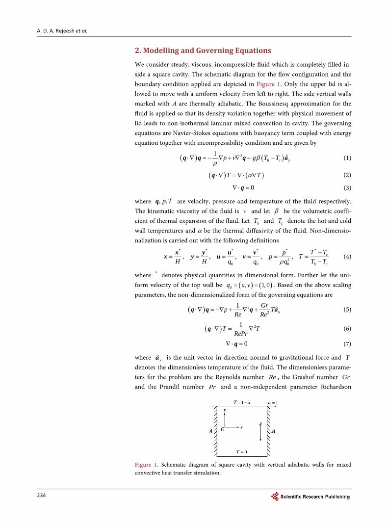
We consider steady, viscous, incompressible fluid which is completely filled in-side a square cavity. The schematic diagram for the flow configuration and the boundary condition applied are depicted in Figure 1. Only the upper lid is al-lowed to move with a uniform velocity from left to right. The side vertical walls marked with A are thermally adiabatic. The Boussinesq approximation for the fluid is applied so that its density variation together with physical movement of lid leads to non-isothermal laminar mixed convection in cavity. The governing equations are Navier-Stokes equations with buoyancy term coupled with energy equation together with incompressibility condition and are given by

( ) ( )21 ˆh c yp g T Tν βρ

⋅∇ = − ∇ + ∇ + −q q q a (1)

( ) ( )T Tα⋅∇ = ∇ ⋅ ∇q (2)

0∇ ⋅ =q (3)

where , ,p Tq are velocity, pressure and temperature of the fluid respectively. The kinematic viscosity of the fluid is ν and let β be the volumetric coeffi-cient of thermal expansion of the fluid. Let hT and cT denote the hot and cold wall temperatures and α be the thermal diffusivity of the fluid. Non-dimensio- nalization is carried out with the following definitions

** * * * *

20 0 0

, , , , , c

h c

T Tpp TH H q q T Tqρ

−= = = = = =

−x y u vx y u v (4)

where * denotes physical quantities in dimensional form. Further let the uni-form velocity of the top wall be ( ) ( )0 , 1,0q u v= = . Based on the above scaling parameters, the non-dimensionalized form of the governing equations are

( ) 22

1 ˆGrp TRe Re

⋅∇ = −∇ + ∇ + yq q q a (5)

( ) 21T TRePr

⋅∇ = ∇q (6)

0∇ ⋅ =q (7)

where ˆ ya is the unit vector in direction normal to gravitational force and T denotes the dimensionless temperature of the fluid. The dimensionless parame- ters for the problem are the Reynolds number Re , the Grashof number Gr and the Prandtl number Pr and a non-independent parameter Richardson

Figure 1. Schematic diagram of square cavity with vertical adiabatic walls for mixed convective heat transfer simulation.

234

A. D. A. Rejeesh et al.

number Ri . In the stream function-vorticity or ψ-ω formulation, the governing equations become

2 2

2 2x yψ ψ ω∂ ∂

+ = −∂ ∂

(8)

2 2

2 21 Tu v Ri

x y Re xx yω ω ω ω ∂ ∂ ∂ ∂ ∂+ = + + ∂ ∂ ∂∂ ∂

(9)

2 2

2 21T T T Tu v

x y RePr x y ∂ ∂ ∂ ∂

+ = + ∂ ∂ ∂ ∂ (10)

where ω is vorticity of the fluid, u and v are defined in terms of streamfunc-tion as

= ∇× qω (11)

uyψ∂

=∂

(12)

vxψ∂

= −∂

(13)

The boundary conditions used in the present case are as follows. Let the hori-zontal and vertical components of velocity q be u and v respectively. Only for the top horizontal wall, 1u = and 0v = is applied. For all other walls,

0u v= = . Also, 0ψ = on all walls. The viscosity of the fluid which is in con-tact with the surface of the wall generates vorticity ω in the fluid, which is given by 2 2nω ψ= −∂ ∂ where n refers to a direction perpendicular to the wall. The boundary conditions for temperature is as follows. A linearly varying tem-perature given by 1T x= − is prescribed for the top moving wall while the bottom horizontal wall is held at fixed temperature given by 0T = . The two vertical walls are held thermodynamically adiabatic which means no heat flux can enter or leave the wall and therefore we have 0T∂ ∂ =n on the vertical walls. Here n refers to a direction normal to the surface of the wall.

3. Discretization Scheme

Here, we describe the discretization procedure for to the governing set of partial differential equations. Let h and k denotes the grid spacing ( )h k≠ then, from Taylor series expansion, we have, the fourth order accurate finite difference re-presentation for the first and second derivatives as follows.

( )2 3

436

hD hξφ φφξ ξ∂ ∂

= − +∂ ∂

(14)

( )2 2 4

2 42 412

hD hξφ φφξ ξ∂ ∂

= − +∂ ∂

(15)

( )2 3

436

kD hηφ φφη η∂ ∂

= − +∂ ∂

(16)

( )2 2 4

2 42 412

hD hηφ φφη η∂ ∂

= − +∂ ∂

(17)

235

A. D. A. Rejeesh et al.

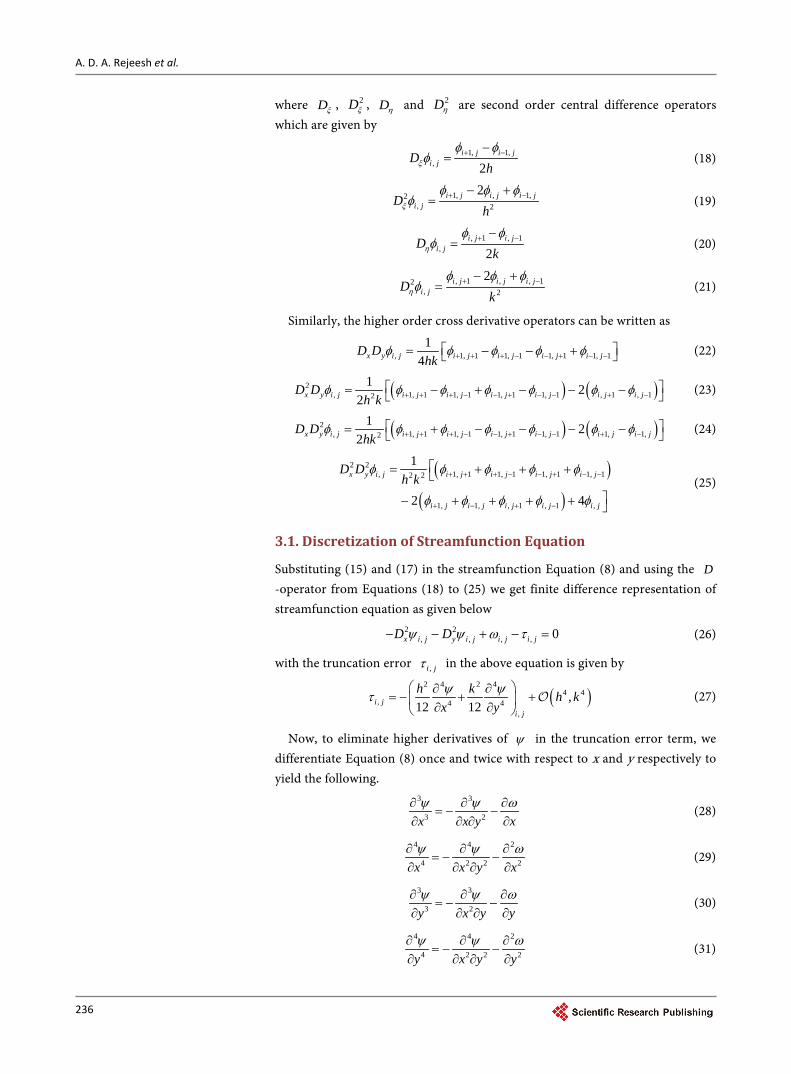
where Dξ , 2Dξ , Dη and 2Dη are second order central difference operators which are given by

1, 1,, 2

i j i ji jD

hξ

φ φφ + −−

= (18)

1, , 1,2, 2

2i j i j i ji jD

hξ

φ φ φφ + −− +

= (19)

, 1 , 1, 2

i j i ji jD

kη

φ φφ + −−

= (20)

, 1 , , 12, 2

2i j i j i ji jD

kη

φ φ φφ + −− +

= (21)

Similarly, the higher order cross derivative operators can be written as

, 1, 1 1, 1 1, 1 1, 11

4x y i j i j i j i j i jD Dhk

φ φ φ φ φ+ + + − − + − − = − − + (22)

( ) ( )2, 1, 1 1, 1 1, 1 1, 1 , 1 , 12

1 22x y i j i j i j i j i j i j i jD D

h kφ φ φ φ φ φ φ+ + + − − + − − + −

= − + − − − (23)

( ) ( )2, 1, 1 1, 1 1, 1 1, 1 1, 1,2

1 22x y i j i j i j i j i j i j i jD D

hkφ φ φ φ φ φ φ+ + + − − + − − + −

= + − − − − (24)

( )( )

2 2, 1, 1 1, 1 1, 1 1, 12 2

1, 1, , 1 , 1 ,

1

2 4

x y i j i j i j i j i j

i j i j i j i j i j

D Dh k

φ φ φ φ φ

φ φ φ φ φ

+ + + − − + − −

+ − + −

= + + +

− + + + +

(25)

3.1. Discretization of Streamfunction Equation

Substituting (15) and (17) in the streamfunction Equation (8) and using the D-operator from Equations (18) to (25) we get finite difference representation of streamfunction equation as given below

2 2, , , , 0x i j y i j i j i jD Dψ ψ ω τ− − + − = (26)

with the truncation error ,i jτ in the above equation is given by

( )2 4 2 4

4 4, 4 4

,

,12 12i j

i j

h k h kx yψ ψτ

∂ ∂= − + +

∂ ∂ (27)

Now, to eliminate higher derivatives of ψ in the truncation error term, we differentiate Equation (8) once and twice with respect to x and y respectively to yield the following.

3 3

3 2 xx x yψ ψ ω∂ ∂ ∂

= − −∂∂ ∂ ∂

(28)

4 4 2

4 2 2 2x x y xψ ψ ω∂ ∂ ∂

= − −∂ ∂ ∂ ∂

(29)

3 3

3 2 yy x yψ ψ ω∂ ∂ ∂

= − −∂∂ ∂ ∂

(30)

4 4 2

4 2 2 2y x y yψ ψ ω∂ ∂ ∂

= − −∂ ∂ ∂ ∂

(31)

236

A. D. A. Rejeesh et al.

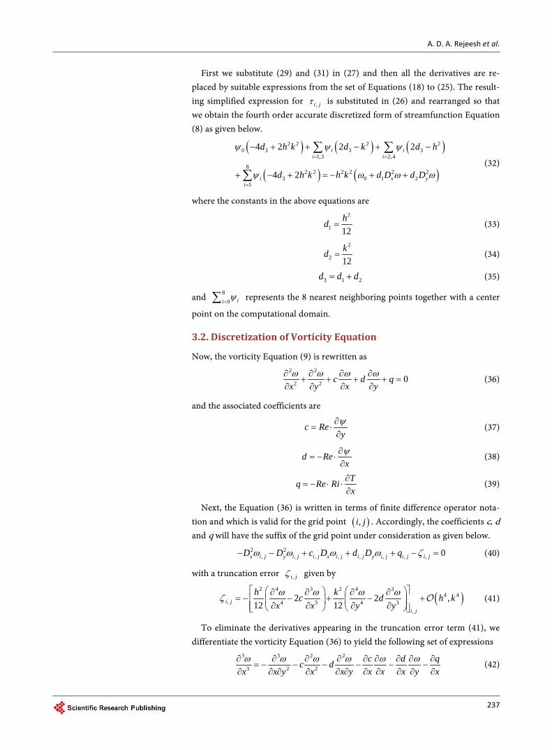
First we substitute (29) and (31) in (27) and then all the derivatives are re-placed by suitable expressions from the set of Equations (18) to (25). The result-ing simplified expression for ,i jτ is substituted in (26) and rearranged so that we obtain the fourth order accurate discretized form of streamfunction Equation (8) as given below.

( ) ( ) ( )

( ) ( )

2 2 2 20 3 3 3

1,3 2,4

82 2 2 2 2 2

3 0 1 25

4 2 2 2

4 2

i ii i

i x yi

d h k d k d h

d h k h k d D d D

ψ ψ ψ

ψ ω ω ω

= =

=

− + + − + −

+ − + = − + +

∑ ∑

∑ (32)

where the constants in the above equations are 2

1 12hd = (33)

2

2 12kd = (34)

3 1 2d d d= + (35)

and 80 ii ψ

=∑ represents the 8 nearest neighboring points together with a center

point on the computational domain.

3.2. Discretization of Vorticity Equation

Now, the vorticity Equation (9) is rewritten as 2 2

2 2 0c d qx yx y

ω ω ω ω∂ ∂ ∂ ∂+ + + + =

∂ ∂∂ ∂ (36)

and the associated coefficients are

c Reyψ∂

= ⋅∂

(37)

d Rexψ∂

= − ⋅∂

(38)

Tq Re Rix

∂= − ⋅ ⋅

∂ (39)

Next, the Equation (36) is written in terms of finite difference operator nota-tion and which is valid for the grid point ( ),i j . Accordingly, the coefficients c, d and q will have the suffix of the grid point under consideration as given below.

2 2, , , , , , , , 0x i j y i j i j x i j i j y i j i j i jD D c D d D qω ω ω ω ζ− − + + + − = (40)

with a truncation error ,i jζ given by

( )2 4 3 2 4 3

4 4, 4 3 4 3

,

2 2 ,12 12i j

i j

h kc d h kx x y yω ω ω ωζ

∂ ∂ ∂ ∂= − − + − +

∂ ∂ ∂ ∂ (41)

To eliminate the derivatives appearing in the truncation error term (41), we differentiate the vorticity Equation (36) to yield the following set of expressions

3 3 2 2

3 2 2c d qc d

x y x x x y xx x y xω ω ω ω ω ω∂ ∂ ∂ ∂ ∂ ∂ ∂ ∂ ∂= − − − − − −

∂ ∂ ∂ ∂ ∂ ∂ ∂∂ ∂ ∂ ∂ (42)

237

A. D. A. Rejeesh et al.

4 4 3 3 22

4 2 2 2 2 2

2 2

2

2 2

2 2

2

2

cc d cxx x y x y x y x

d c ccd cx x y x xx

d d q qc cx y xx x

ω ω ω ω ω

ω ω

ω

∂ ∂ ∂ ∂ ∂ ∂ = − + − + − ∂∂ ∂ ∂ ∂ ∂ ∂ ∂ ∂

∂ ∂ ∂ ∂ ∂ + − + − ∂ ∂ ∂ ∂ ∂∂ ∂ ∂ ∂ ∂ ∂

+ − + − ∂ ∂ ∂∂ ∂

(43)

3 3 2

3 2

2

2

cx yy x y

c d qdy x y y yy

ω ω ω

ω ω ω

∂ ∂ ∂= − −

∂ ∂∂ ∂ ∂

∂ ∂ ∂ ∂ ∂ ∂− − − −

∂ ∂ ∂ ∂ ∂∂

(44)

4 4 3 3 22

4 2 2 2 2 2

2 2

2

2 2

2 2

2

2

dc d dyy x y x y x y y

c c ccd dy x y y xy

d d q qd dy y yy y

ω ω ω ω ω

ω ω

ω

∂ ∂ ∂ ∂ ∂ ∂= − − + + − ∂∂ ∂ ∂ ∂ ∂ ∂ ∂ ∂

∂ ∂ ∂ ∂ ∂+ − + − ∂ ∂ ∂ ∂ ∂∂ ∂ ∂ ∂ ∂ ∂

+ − + − ∂ ∂ ∂∂ ∂

(45)

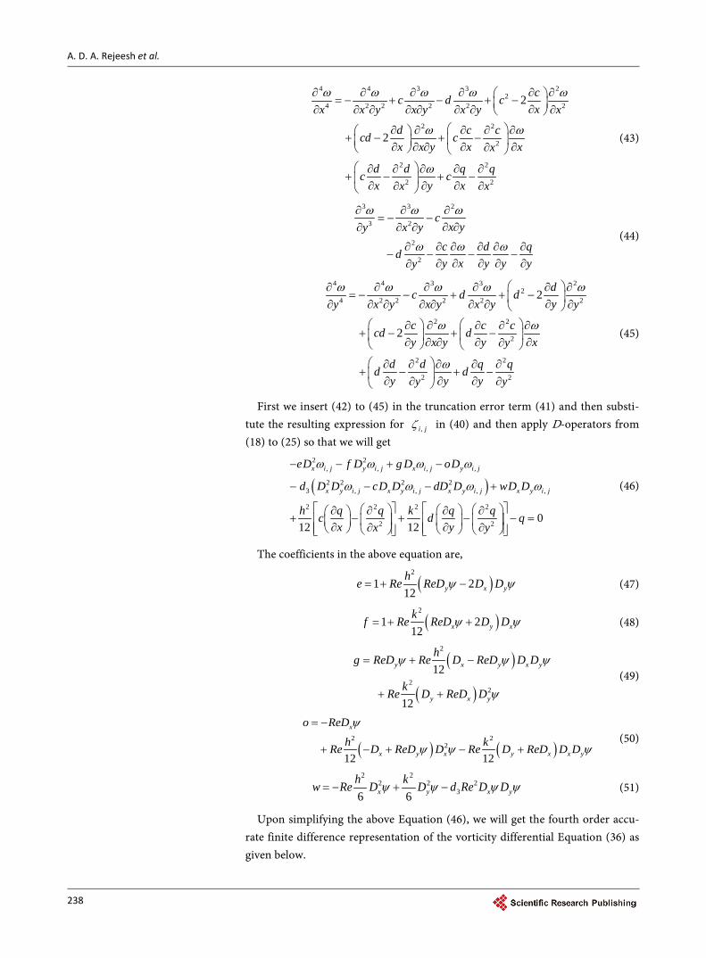
First we insert (42) to (45) in the truncation error term (41) and then substi-tute the resulting expression for ,i jζ in (40) and then apply D-operators from (18) to (25) so that we will get

( )

2 2, , , ,

2 2 2 23 , , , ,

2 2 2 2

2 2 012 12

x i j y i j x i j y i j

x y i j x y i j x y i j x y i j

eD f D g D oD

d D D cD D dD D wD D

h q q k q qc d qx yx y

ω ω ω ω

ω ω ω ω

− − + −

− − − +

∂ ∂ ∂ ∂ + − + − − = ∂ ∂∂ ∂

(46)

The coefficients in the above equation are,

( )2

1 212 y x yhe Re ReD D Dψ ψ= + − (47)

( )2

1 212 x y xkf Re ReD D Dψ ψ= + + (48)

( )

( )

2

22

12

12

y x y x y

y x y

hg ReD Re D ReD D D

kRe D ReD D

ψ ψ ψ

ψ

= + −

+ + (49)

( ) ( )2 2

2

12 12

x

x y x y x x y

o ReD

h kRe D ReD D Re D ReD D D

ψ

ψ ψ ψ

= −

+ − + − + (50)

2 22 2 2

36 6x y x yh kw Re D D d Re D Dψ ψ ψ ψ= − + − (51)

Upon simplifying the above Equation (46), we will get the fourth order accu-rate finite difference representation of the vorticity differential Equation (36) as given below.

238

A. D. A. Rejeesh et al.

( ) ( )( ) ( )( ) ( )( ) ( )

2 2 2 20 3 1 3 3

2 2 2 22 3 3 3 3 3

2 24 3 3 5 3 3 3

6 3 3 3 7 3 3 3

8 3 3 3

16 8 8 8 4 4 2

8 4 4 2 8 4 4 2

8 4 4 2 4 2 2

4 2 2 4 2 2

4 2 2

d h f k e d hd c k e hk g

d kd d h f h ko d hd c k e hk g

d kd d h f h ko d hd c kd d hkw

d hd c kd d hkw d hd c kd d hkw

d hd c kd d hk

ω ω

ω ω

ω ω

ω ω

ω

− + + + − − +

+ − − + + + − −

+ + − − + − + + +

+ − − + − + − − − +

+ − + − −( )

( ) ( )2 2

2 2 2 24 112 12y x x y Y x

w

h kh k Re Ri ReD D ReD D D D Tψ ψ

= − ⋅ − + + + +

(52)

It may be noted that before implementing the code for Equation (10), the ex-pressions for the quantities c, d and q should also be replaced by fourth order accurate relations as given below.

32

, 2 2 23i j y y x y yc Re D d Re D d D D Re d Dyψψ ψ ω

∂ = − = + − ∂ (53)

[ ]3

2, 1 1 13i j x x y x xd Re Pr D d Re D d D D Re d D

xψψ ψ ω

∂ = − ⋅ − = − + − ∂ (54)

[ ]3

2, 1 1 13i j x x y x x

Tq Re Pr D d Re Pr D d D D T Re Pr d Dx

ψ ω ∂ = − ⋅ − = − ⋅ + − ⋅ ∂

(55)

3.3. Discretization of Energy Equation

Now, the temperature Equation (10) is rewritten as 2 2

2 2 0T T T Tc dx yx y

∂ ∂ ∂ ∂′ ′+ + + =∂ ∂∂ ∂

(56)

Let us define primed variables c′ and d ′ at the grid point ( ),i j as

2Re Prc

yψ ⋅ ∂′ = − ∂

(57)

2Re Prd

xψ⋅ ∂ ′ = ∂

(58)

Using Equations (14) to (17) together with the above two primed variables in (10), we get discretized version with truncation error term as follows.

2 2, , , , , , , 0x i j y i j i j x i j i j y i j i jD T D T c D T d D T γ′ ′+ + + − = (59)

and the truncation error term ,i jγ in the previous equation is

( )

2 3 2 4 2 3 2 4

, 3 4 3 4,

4 4

6 12 6 12

,

i ji j

c h T h T d k T k Tx x y y

h k

γ ′ ′∂ ∂ ∂ ∂

= − + + + ∂ ∂ ∂ ∂

+

(60)

Now the higher order derivatives of T present in the previous expression for truncation error can be eliminated by differentiating the energy Equation (10) with respect to x and y to yield the following.

3 3 2 2

3 2 2

T T T T c T d Tc dx y x x x yx x y x

′ ′∂ ∂ ∂ ∂ ∂ ∂ ∂ ∂′ ′= − − − − −∂ ∂ ∂ ∂ ∂ ∂∂ ∂ ∂ ∂

(61)

239

A. D. A. Rejeesh et al.

( )4 4 3 3 2

24 2 2 2 2 2

2 2 2

2 2

2

2'

T T T T c Tc d cxx x y x y x y x

d T c c T d d Tc d c cx x y x x x yx x

′∂ ∂ ∂ ∂ ∂ ∂ ′ ′ ′= − + − + − ∂∂ ∂ ∂ ∂ ∂ ∂ ∂ ∂

′ ′ ′ ′ ′∂ ∂ ∂ ∂ ∂ ∂ ∂ ∂ ′ ′ ′+ − + − + − ∂ ∂ ∂ ∂ ∂ ∂ ∂∂ ∂

(62)

3 3 2 2

3 2 2

T T T T c T d Tc dx y y x y yy x y y

′ ′∂ ∂ ∂ ∂ ∂ ∂ ∂ ∂′ ′= − − − − −∂ ∂ ∂ ∂ ∂ ∂∂ ∂ ∂ ∂

(63)

( )4 4 3 3 2

24 2 2 2 2 2

2 2 2

2 2

2

2

T T T T d Tc d dyy x y x y x y y

c T c c T d d Tc d d dy x y y x y yy y

′ ∂ ∂ ∂ ∂ ∂ ∂′ ′ ′= − − + + − ∂∂ ∂ ∂ ∂ ∂ ∂ ∂ ∂ ′ ′ ′ ′ ′ ∂ ∂ ∂ ∂ ∂ ∂ ∂ ∂′ ′ ′ ′+ − + − + − ∂ ∂ ∂ ∂ ∂ ∂ ∂∂ ∂

(64)

Substituting the set of Equations (61) to (64) in the equation for truncation error (60) and also applying the D operators from (18) to (25), in the Equation (59) we get

( )

2 2

2 2 2 21 2 0

x y x y x y

x y x y x y

D D D D D D T

d d D D c D D d D D T

ς ρ ϖ ϑ ε − − + + + ′ ′− + − − =

(65)

where the coefficients ς , ρ , ϖ , ϑ , ε appearing in the above equation are

( )21 11 x yd c Re Pr d D Dς ψ′= + − ⋅ ⋅ (66)

( )2 22 21 yd d Re Pr d Dρ ψ′= + − ⋅ ⋅ (67)

( ) ( )2 21 2x x y yc d c D c D c d d D c D cϖ ′ ′ ′ ′ ′ ′ ′= + + + + (68)

( ) ( )2 21 2x x y yd d c D d D d d d D d D dϑ ′ ′ ′ ′ ′ ′ ′= + + + + (69)

( ) ( )2 21 2 1 2x yRe Pr d D d D d d c dε ψ ′ ′= ⋅ − + − + ⋅ (70)

It may be noted that before implementing the code for Equation (65), the ex-pressions for primed quantities c′ and d ′ should also be replaced by fourth order accurate relations as given below.

( )3

2 3,

22 2

yi j

y y x y

c Re Pr D dy

Re Pr d D Re Pr D d D D

ψψ

ω ψ

∂′ = − ⋅ − ∂

= ⋅ − ⋅ +

(71)

( )

[ ]

3

1 3,

21 1

xi j

x x y x

d Re Pr D dx

Re Pr d D Re Pr D d D D

ψψ

ω ψ

∂′ = ⋅ − ∂ = ⋅ + ⋅ +

(72)

and the constants 1d , 2d and 3d are already defined in Equations (33) to (35). Finally, we have arrived at a set of three coupled discretized Equations (32), (52) and (65) whose accuracy is ( )4 4,h k .

4. Implementation of Numerical Scheme

The set of coupled discretized equations as mentioned above is applied to each grid point in the computational domain and this produces a large linear sparse

240

A. D. A. Rejeesh et al.

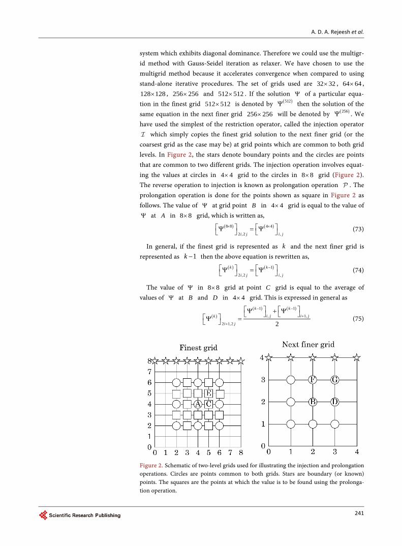
system which exhibits diagonal dominance. Therefore we could use the multigr-id method with Gauss-Seidel iteration as relaxer. We have chosen to use the multigrid method because it accelerates convergence when compared to using stand-alone iterative procedures. The set of grids used are 32 32× , 64 64× , 128 128× , 256 256× and 512 512× . If the solution Ψ of a particular equa-tion in the finest grid 512 512× is denoted by ( )512Ψ then the solution of the same equation in the next finer grid 256 256× will be denoted by ( )256Ψ . We have used the simplest of the restriction operator, called the injection operator which simply copies the finest grid solution to the next finer grid (or the coarsest grid as the case may be) at grid points which are common to both grid levels. In Figure 2, the stars denote boundary points and the circles are points that are common to two different grids. The injection operation involves equat-ing the values at circles in 4 4× grid to the circles in 8 8× grid (Figure 2). The reverse operation to injection is known as prolongation operation . The prolongation operation is done for the points shown as square in Figure 2 as follows. The value of Ψ at grid point B in 4 4× grid is equal to the value of Ψ at A in 8 8× grid, which is written as,

( ) ( )8 8 4 4

2 ,2 ,i j i j

× × Ψ = Ψ (73)

In general, if the finest grid is represented as k and the next finer grid is represented as 1k − then the above equation is rewritten as,

( ) ( )1

2 ,2 ,

k k

i j i j

− Ψ = Ψ (74)

The value of Ψ in 8 8× grid at point C grid is equal to the average of values of Ψ at B and D in 4 4× grid. This is expressed in general as

( )( ) ( )1 1

, 1,

2 1,2 2

k k

i j i jk

i j

− −

+

+

Ψ + Ψ Ψ = (75)

Figure 2. Schematic of two-level grids used for illustrating the injection and prolongation operations. Circles are points common to both grids. Stars are boundary (or known) points. The squares are the points at which the value is to be found using the prolonga- tion operation.

241

A. D. A. Rejeesh et al.

Here k means finest grid and 1k − means next finer (or coarsest) grid. Si-milarly, the values at all other square points are obtained using the following av-eraging scheme.

( ) ( ) ( )1 1

2 ,2 1 , , 1

12

k k k

i j i j i j

− −

+ +

Ψ = Ψ + Ψ (76)

( ) ( ) ( )

( ) ( )

1 1

2 1,2 1 , 1,

1 1

, 1 1, 1

14

k k k

i j i j i j

k k

i j i j

− −

+ + +

− −

+ + +

Ψ = Ψ + Ψ + Ψ + Ψ

(77)

The above set of Equations (74) to (77) comprise the 9-point prolongation operator [38]. The three coupled discretized Equations (32), (52) and (65) are relaxed simultaneously and the boundary conditions are incorporated implicitly. A point Gauss-Seidel iterative scheme is used for the relaxation procedure. This pre-smoothing iterations are carried out on the finest grid. Then we restrict (or inject) the residual on the coarsest grid. Let the residual be denoted by r . By solving the matrix equation Ae r= we get the error in the coarsest grid. This error e is prolongated to the finest grid and then added to oldΨ as below

[ ]coarse grid corrected old eΨ = Ψ + (78)

where is the prolongation operator (for more details, see [38]). After per-forming a few post-smoothing operation, one multigrid cycle is completed. This procedure is repeated until the following condition is satisfied for convergence.

17

110

n n

n

X X

X

+−

+

−≤ (79)

where X is any of , ,Tψ ω and n is the iteration number.

Treatment of Boundary Points

At all the boundary points, fourth order accurate one sided finite-difference formula is used for derivatives involving ,ψ ω and T . The first derivative of temperature along all points in left vertical wall is

( ) ( ) ( ) ( ) ( )11, 48 2, 36 3, 16 4, 3 5,25

T j T j T j T j T j= − + − (80)

and similarly the same for the right vertical wall is expressed as

( ) ( ) ( ) ( ) ( )11, 48 , 36 1, 16 2, 3 3,25

T m j T m j T m j T m j T m j+ = − + − − − + − (81)

A fourth order backward difference scheme is used to find ω at top moving wall.

( ) ( ) ( ) ( )

( ) ( ) ( )2

1, 1 45 , 1 154 , 214 , 112

156 , 2 61 , 3 10 , 4

i n i n i n i nh

i n i n i n

ω ψ ψ ψ

ψ ψ ψ

−+ = + − + −

− − + − − −

(82)

Similarly, the fourth order one sided finite difference is used to find ω at all other walls

242

A. D. A. Rejeesh et al.

( ) ( ) ( ) ( )

( ) ( ) ( )2

11, 45 1, 154 2, 214 3,12

156 4, 61 5, 10 6,

j j j jh

j j j

ω ψ ψ ψ

ψ ψ ψ

−= − +

− + −

(83)

( ) ( ) ( ) ( )

( ) ( ) ( )2

11, 45 1, 154 , 214 1,12

156 2, 61 3, 10 4,

m j m j m j m jh

m j m j m j

ω ψ ψ ψ

ψ ψ ψ

−+ = + − + −

− − + − − −

(84)

( ) ( ) ( )

( ) ( ) ( )2

1,1 45 ( ,1) 154 ,2 214 ,312

156 ,4 61 ,5 10 ,6

i i i ih

i i i

ω ψ ψ ψ

ψ ψ ψ

−= − +

− + −

(85)

5. Results and Discussion

The flow characteristics together with thermal fields are computed for different Re , Pr and Gr (or equivalent Ri ). The density variation is induced through a linearly varying top moving wall. The effect of mixed convection is analyzed through streamlines, isothermal contours and Nusselt number for 100 3000Re≤ ≤ , 0.015 10Pr≤ ≤ and Grashof number 2 610 10Gr≤ ≤ and further explained through contours of components of velocity and temperature in the mid-cross-section of the cavity. At the end, the numerical accuracy of the proposed scheme is established.

5.1. Code Validation and Grid Independence Study

To validate our coding we have run the program with aiding and opposing shear boundary conditions available in the literature. The validations are done for various values of Re and a fixed value of 0.73Pr = . The parameter used to study the mixed convection is Richardson number Ri which is also equal to

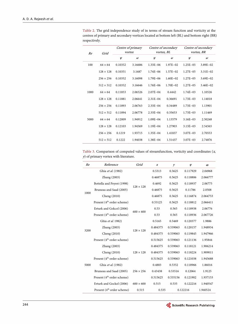
2Gr Re . The case of 1Ri belongs to the class of forced convection and if 0.1 10Ri≤ ≤ we may describe as mixed convection. Table 2 shows the grid in-dependence results for 0Gr = case in terms of values of streamfunction, ψ , and vorticity, ω which are evaluated at the centers of primary and two sec-ondary vortices for different values of Re . Here a fluid with a constant

0.73Pr = is considered. In our computation, the coarser grids are 64 64× , 128 128× , and 256 256× while the finest grid used in the present study is 512 512× . From the tabulated data, it is seen that 256 256× grid is found to be optimum. Further refining of grids will not give more accuracy because the ac-curacy of the numerical scheme is decided by method of discretization and not by the fineness of the grid. The advantage with the present higher order scheme is that we can achieve the accurate results in smaller grid itself. Table 3 shows the location of primary vortex and flow parameters such as streamfunction and vorticity in different grids, and they are compared with the literature data that include data that might have been computed using a lower order finite difference method [1] [13] [14] [39] [40] [41], and from the tabulated data it is observed that there is a very good agreement among different reports. In particular, the results of [14] is matching to a good degree with that of our computed value. In

243

A. D. A. Rejeesh et al.

Table 2. The grid independence study of in terms of stream function and vorticity at the centres of primary and secondary vortices located at bottom left (BL) and bottom right (BR) respectively.

Re Grid

Centre of primary vortex

Centre of secondary vortex, BL

Centre of secondary vortex, BR

ψ ω ψ ω ψ ω

100 64 × 64 0.10352 3.16686 1.33E−06 1.97E−02 1.25E−05 3.89E−02

128 × 128 0.10351 3.1687 1.74E−06 1.57E−02 1.27E−05 3.31E−02

256 × 256 0.10352 3.16098 1.79E−06 1.60E−02 1.27E−05 3.69E−02

512 × 512 0.10352 3.16646 1.76E−06 1.70E−02 1.27E−05 3.46E−02

1000 64 × 64 0.11853 2.06526 2.07E−04 0.4442 1.74E−03 1.10526

128 × 128 0.11881 2.06641 2.31E−04 0.36691 1.73E−03 1.14018

256 × 256 0.11893 2.06763 2.33E−04 0.34489 1.73E−03 1.13901

512 × 512 0.11894 2.06778 2.33E−04 0.35653 1.73E−03 1.11469

5000 64 × 64 0.12009 1.94912 1.09E−04 1.13579 3.16E−03 2.50248

128 × 128 0.12103 1.94569 1.19E−04 1.27903 3.13E−03 2.54565

256 × 256 0.1219 1.93715 1.35E−04 1.41837 3.07E−03 2.70553

512 × 512 0.1222 1.94038 1.38E−04 1.51437 3.07E−03 2.74876

Table 3. Comparison of computed values of streamfunction, vorticity and coordinates (x, y) of primary vortex with literature.

Re Reference Grid x y ψ ω

1000

Ghia et al. (1982)

128 × 128

0.5313 0.5625 0.117929 2.04968

Zhang (2003) 0.46875 0.5625 0.118806 2.066777

Bottella and Peyret (1998) 0.4692 0.5625 0.118937 2.06775

Bruneau and Saad (2005) 0.46875 0.5625 0.11786 2.0508

Cheng (2010) 0.46875 0.5625 0.116874 2.064753

Present (4th order scheme) 0.53125 0.5625 0.118812 2.066411

Erturk and Gokcol (2006) 600 × 600

0.53 0.565 0.118938 2.06776

Present (4th order scheme) 0.53 0.565 0.118936 2.067726

3200

Ghia et al. 1982)

128 × 128

0.5165 0.5469 0.120377 1.9886

Zhang (2003) 0.484375 0.539063 0.120157 1.948934

Cheng (2010) 0.484375 0.539063 0.119845 1.947966

Present (4th order scheme) 0.515625 0.539063 0.121136 1.95844

5000

Zhang (2003)

128 × 128

0.484375 0.539063 0.118121 1.906214

Cheng (2010) 0.484375 0.539063 0.118224 1.909011

Present (4th order scheme) 0.515625 0.539063 0.121038 1.945688

Ghia et al. (1982)

256 × 256

0.4883 0.5352 0.118966 1.86016

Bruneau and Saad (2005) 0.43438 0.53516 0.12064 1.9125

Present (4th order scheme) 0.515625 0.535156 0.121902 1.937153

Erturk and Gockol (2006) 600 × 600 0.515 0.535 0.122216 1.940547

Present (4th order scheme) 0.515 0.535 0.122216 1.940524

244

A. D. A. Rejeesh et al.

order to perform validation for heat transfer studies, we have exclusively run the code with the boundary condition 1T = for the top moving wall and the re-sults are shown in Table 4 and the data is compared with literature [15] [42] [43]. Essentially there is hardly a 0.03% variation among other reported values that has been computed using some fourth order scheme and 0.1% variation among second order accurate computations.

5.2. Flow Structure and Isotherms

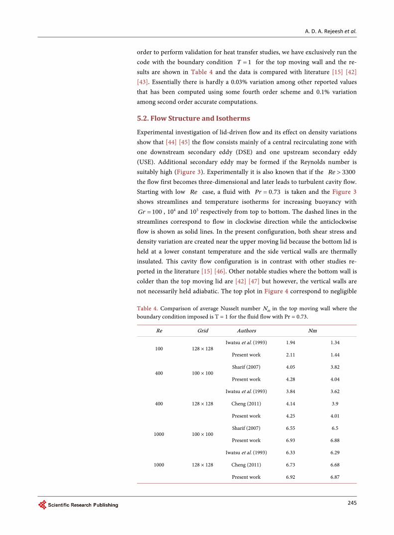
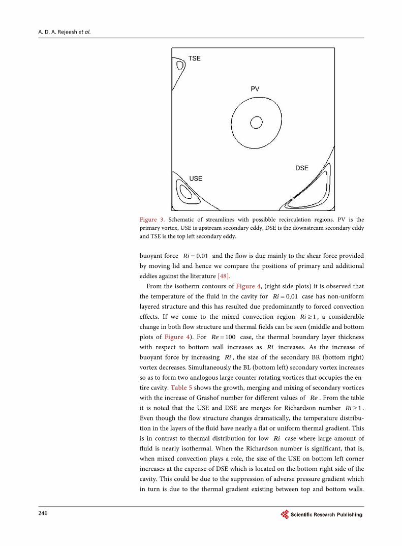
Experimental investigation of lid-driven flow and its effect on density variations show that [44] [45] the flow consists mainly of a central recirculating zone with one downstream secondary eddy (DSE) and one upstream secondary eddy (USE). Additional secondary eddy may be formed if the Reynolds number is suitably high (Figure 3). Experimentally it is also known that if the 3300Re > the flow first becomes three-dimensional and later leads to turbulent cavity flow. Starting with low Re case, a fluid with 0.73Pr = is taken and the Figure 3 shows streamlines and temperature isotherms for increasing buoyancy with

100Gr = , 104 and 105 respectively from top to bottom. The dashed lines in the streamlines correspond to flow in clockwise direction while the anticlockwise flow is shown as solid lines. In the present configuration, both shear stress and density variation are created near the upper moving lid because the bottom lid is held at a lower constant temperature and the side vertical walls are thermally insulated. This cavity flow configuration is in contrast with other studies re-ported in the literature [15] [46]. Other notable studies where the bottom wall is colder than the top moving lid are [42] [47] but however, the vertical walls are not necessarily held adiabatic. The top plot in Figure 4 correspond to negligible Table 4. Comparison of average Nusselt number Nm in the top moving wall where the boundary condition imposed is T = 1 for the fluid flow with Pr = 0.73.

Re Grid Authors Nm

100 128 × 128 Iwatsu et al. (1993) 1.94 1.34

Present work 2.11 1.44

400 100 × 100 Sharif (2007) 4.05 3.82

Present work 4.28 4.04

400 128 × 128

Iwatsu et al. (1993) 3.84 3.62

Cheng (2011) 4.14 3.9

Present work 4.25 4.01

1000 100 × 100 Sharif (2007) 6.55 6.5

Present work 6.93 6.88

1000 128 × 128

Iwatsu et al. (1993) 6.33 6.29

Cheng (2011) 6.73 6.68

Present work 6.92 6.87

245

A. D. A. Rejeesh et al.

Figure 3. Schematic of streamlines with possibble recirculation regions. PV is the primary vortex, USE is upstream secondary eddy, DSE is the downstream secondary eddy and TSE is the top left secondary eddy. buoyant force 0.01Ri = and the flow is due mainly to the shear force provided by moving lid and hence we compare the positions of primary and additional eddies against the literature [48].

From the isotherm contours of Figure 4, (right side plots) it is observed that the temperature of the fluid in the cavity for 0.01Ri = case has non-uniform layered structure and this has resulted due predominantly to forced convection effects. If we come to the mixed convection region 1Ri ≥ , a considerable change in both flow structure and thermal fields can be seen (middle and bottom plots of Figure 4). For 100Re = case, the thermal boundary layer thickness with respect to bottom wall increases as Ri increases. As the increase of buoyant force by increasing Ri , the size of the secondary BR (bottom right) vortex decreases. Simultaneously the BL (bottom left) secondary vortex increases so as to form two analogous large counter rotating vortices that occupies the en-tire cavity. Table 5 shows the growth, merging and mixing of secondary vortices with the increase of Grashof number for different values of Re . From the table it is noted that the USE and DSE are merges for Richardson number 1Ri ≥ . Even though the flow structure changes dramatically, the temperature distribu-tion in the layers of the fluid have nearly a flat or uniform thermal gradient. This is in contrast to thermal distribution for low Ri case where large amount of fluid is nearly isothermal. When the Richardson number is significant, that is, when mixed convection plays a role, the size of the USE on bottom left corner increases at the expense of DSE which is located on the bottom right side of the cavity. This could be due to the suppression of adverse pressure gradient which in turn is due to the thermal gradient existing between top and bottom walls.

246

A. D. A. Rejeesh et al.

Figure 4. Streamfunction contours (left) and isotherms (right) for 0.01,1Ri = and 10 respectively (top to bottom) for a flow of fluid with 100Re = and 0.73Pr = . Equivalent values of Gr are 102, 104 and 105 respectively from top to bottom. Table 5. Growth, degradation and merging of secondary vortices due to increased mixed convection.

Re Gr Ri Area of USE Area of DSE Area of TSE

100

102 0.01 0.28E−2 0.98E−2 0

104 1 2.10E−2 0.78E−2 0

106 10 USE and DSE merges

400

104 0.0625 0.90E−2 3.70E−2 0

105 0.625 4.50E−2 2.60E−2 0

106 6.25 USE and DSE merges

1000

104 0.01 1.90E−2 5.20E−2 0

105 0.1 2.10E−2 4.90E−2 0

106 1 USE and DSE merges

3000

103 0.0011 3.60E−2 7.00E−2 0.080E−2

104 0.011 3.70E−2 6.60E−2 0.085E−2

105 0.11 4.30E−2 5.70E−2 0.090E−2

247

A. D. A. Rejeesh et al.

When Richardson number is increased to 10Ri = , a significant change in the fluid flow is observed, wherein the USE grows until it occupies nearly half of the cavity, which is attributed to the buoyancy effects. The direction of flow in this eddy is opposite to that of the main or primary vortex. In addition, the center of primary vortex moves towards the right wall as Ri increases. The size of the clockwise and anticlockwise rotating vortices have same size, which shows that the effect of shear driven forced convection effect and buoyancy driven convec-tion effects shows equal strength. The thermal contours have more shift than

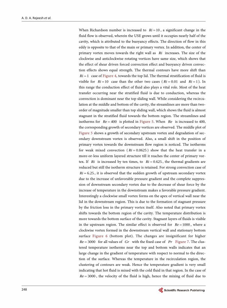
1Ri = case of Figure 4, towards the top lid. The thermal stratification of fluid is visible for 10Ri = case than the other two cases ( 0.01Ri = and 1Ri = ). In this range the conduction effect of fluid also plays a vital role. Most of the heat transfer occurring near the stratified fluid is due to conduction, whereas the convection is dominant near the top sliding wall. While considering the recircu-lation at the middle and bottom of the cavity, the streamlines are more than two- order of magnitude smaller than top sliding wall, which shows the fluid is almost stagnant in the stratified fluid towards the bottom region. The streamlines and isotherms for 400Re = is plotted in Figure 5. When Re is increased to 400, the corresponding growth of secondary vortices are observed. The middle plot of Figure 5 shows a growth of secondary upstream vortex and degradation of sec-ondary downstream vortex is observed. Also, a small shift in the position of primary vortex towards the downstream flow region is noticed. The isotherms for weak mixed convection ( 0.0625Ri = ) show that the heat transfer in a more-or-less uniform layered structure till it reaches the center of primary vor-tex. If Ri is increased by ten times, to 0.625Ri = , the thermal gradients are reduced but still the isotherm structure is retained. For strong convection case of

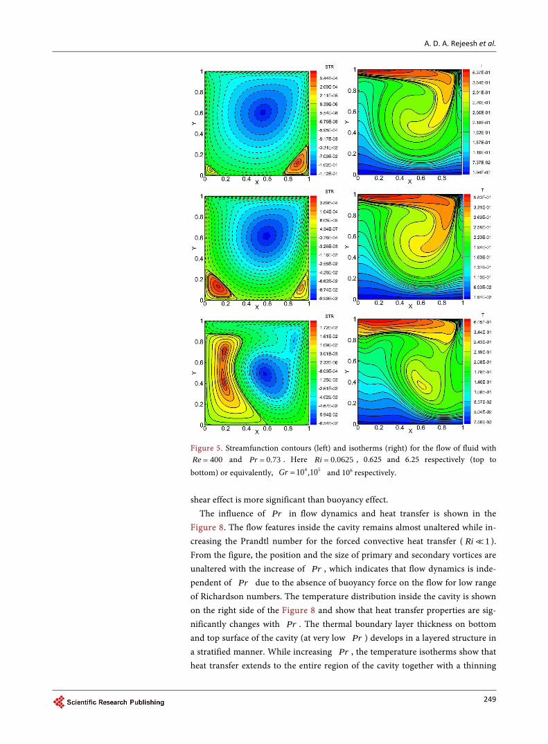
6.25Ri = , it is observed that the sudden growth of upstream secondary vortex due to the increase of unfavorable pressure gradient and the complete suppres-sion of downstream secondary vortex due to the decrease of shear force by the increase of temperature in the downstream makes a favorable pressure gradient. Interestingly a clockwise small vortex forms on the apex of vertical wall near the lid in the downstream region. This is due to the formation of stagnant pressure by the friction loss in the primary vortex itself. Also noted that primary vortex shifts towards the bottom region of the cavity. The temperature distribution is more towards the bottom surface of the cavity. Stagnant layers of fluids is visible in the upstream region. The similar effect is observed for 1000Re = , where a clockwise vortex formed in the downstream vertical wall and stationary bottom surface Figure 6 (bottom plot). The changes are insignificant for higher

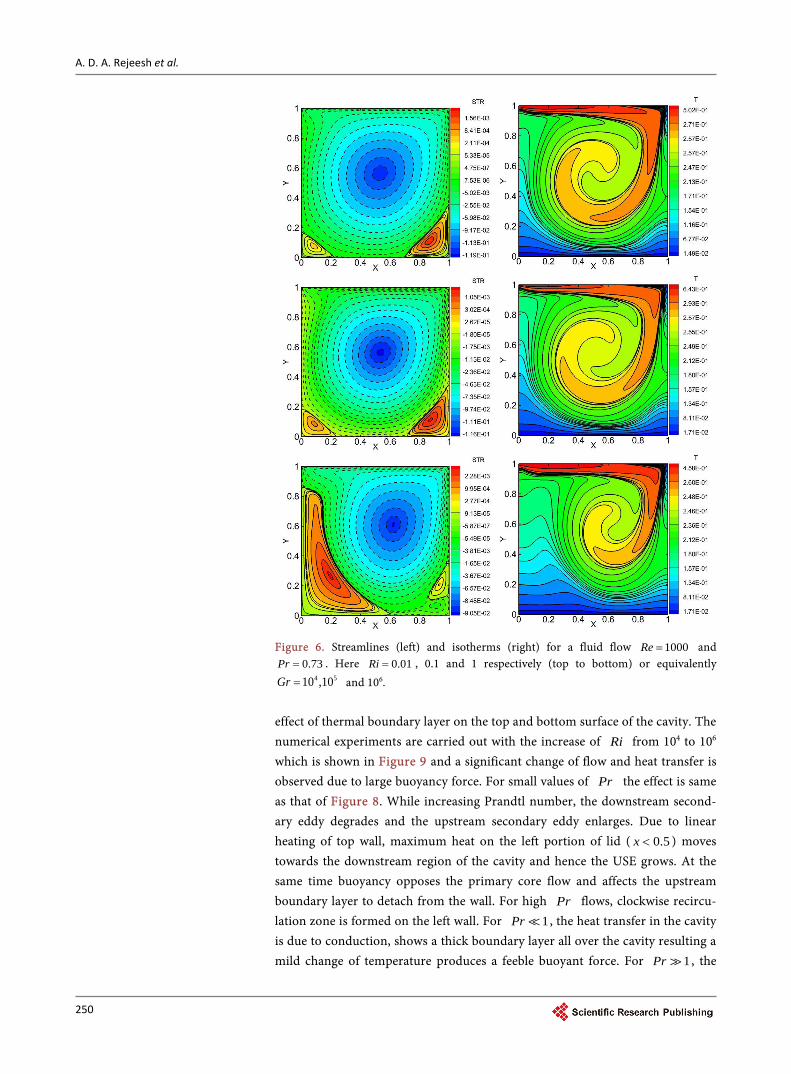
3000Re = for all values of Gr with the fixed case of Pr Figure 7. The clus-tered temperature isotherms near the top and bottom walls indicates that an large change in the gradient of temperature with respect to normal to the direc-tion of the surface. Whereas the temperature in the recirculation region, the clustering of contours are weak. Hence the temperature gradient is very small indicating that hot fluid is mixed with the cold fluid in that region. In the case of

3000Re = , the velocity of the fluid is high, hence the mixing of fluid due to

248

A. D. A. Rejeesh et al.

Figure 5. Streamfunction contours (left) and isotherms (right) for the flow of fluid with

400Re = and 0.73Pr = . Here 0.0625Ri = , 0.625 and 6.25 respectively (top to bottom) or equivalently, 4 510 ,10Gr = and 106 respectively. shear effect is more significant than buoyancy effect.

The influence of Pr in flow dynamics and heat transfer is shown in the Figure 8. The flow features inside the cavity remains almost unaltered while in-creasing the Prandtl number for the forced convective heat transfer ( 1Ri ). From the figure, the position and the size of primary and secondary vortices are unaltered with the increase of Pr , which indicates that flow dynamics is inde-pendent of Pr due to the absence of buoyancy force on the flow for low range of Richardson numbers. The temperature distribution inside the cavity is shown on the right side of the Figure 8 and show that heat transfer properties are sig-nificantly changes with Pr . The thermal boundary layer thickness on bottom and top surface of the cavity (at very low Pr ) develops in a layered structure in a stratified manner. While increasing Pr , the temperature isotherms show that heat transfer extends to the entire region of the cavity together with a thinning

249

A. D. A. Rejeesh et al.

Figure 6. Streamlines (left) and isotherms (right) for a fluid flow 1000Re = and

0.73Pr = . Here 0.01Ri = , 0.1 and 1 respectively (top to bottom) or equivalently 4 510 ,10Gr = and 106.

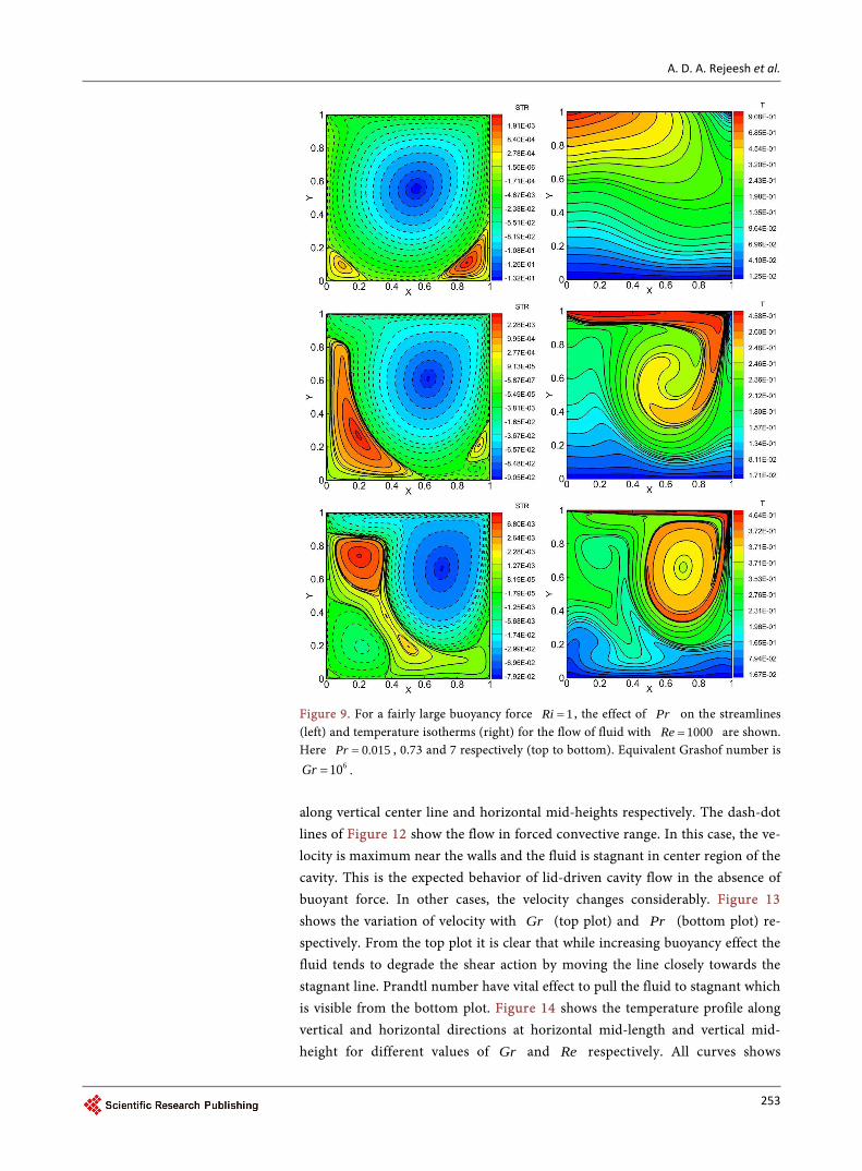
effect of thermal boundary layer on the top and bottom surface of the cavity. The numerical experiments are carried out with the increase of Ri from 104 to 106 which is shown in Figure 9 and a significant change of flow and heat transfer is observed due to large buoyancy force. For small values of Pr the effect is same as that of Figure 8. While increasing Prandtl number, the downstream second-ary eddy degrades and the upstream secondary eddy enlarges. Due to linear heating of top wall, maximum heat on the left portion of lid ( 0.5x < ) moves towards the downstream region of the cavity and hence the USE grows. At the same time buoyancy opposes the primary core flow and affects the upstream boundary layer to detach from the wall. For high Pr flows, clockwise recircu-lation zone is formed on the left wall. For 1Pr , the heat transfer in the cavity is due to conduction, shows a thick boundary layer all over the cavity resulting a mild change of temperature produces a feeble buoyant force. For 1Pr , the

250

A. D. A. Rejeesh et al.

Figure 7. Streamlines (left) and isotherms (right) for a fluid flow with 3000Re = and

0.73Pr = . Here 0.0011Ri = , 0.011 and 0.11 respectively (top to bottom) or equivalently 3 410 ,10Gr = and 105. heat transfer is mainly due to convective effect and the fluid is well mixed in the core of the cavity, hence the buoyant effect exhibits near the walls of the cavity. This makes the degradation of downstream eddy and upgradation of upstream secondary vortex. The reverse will happens for a gravitationally unstable condi-tion [46], where they observed the degradation of upstream secondary vortex and growth of downstream secondary vortex.

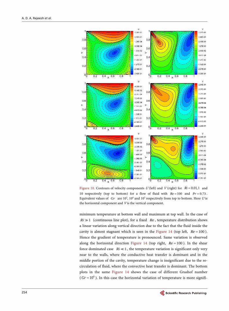
Contours of the horizontal and vertical components of velocity u and v are plotted in Figure 10 and Figure 11 for 100Re = and 1000 respectively. In the case of 100Re = (Figure 10), we could see that the vertical components of ve-locity V is modified to a great extent in the left half of the cavity because of the nature of buoyancy which is ( )1 x− in our case. Consequently, the density variations are more in left half and they are least in the right half of the cavity. This leads a way to develop two large circulations in opposite directions as seen in

251

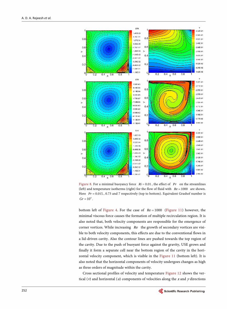
A. D. A. Rejeesh et al.

Figure 8. For a minimal buoyancy force 0.01Ri = , the effect of Pr on the streamlines (left) and temperature isotherms (right) for the flow of fluid with 1000Re = are shown. Here 0.015Pr = , 0.73 and 7 respectively (top to bottom). Equivalent Grashof number is

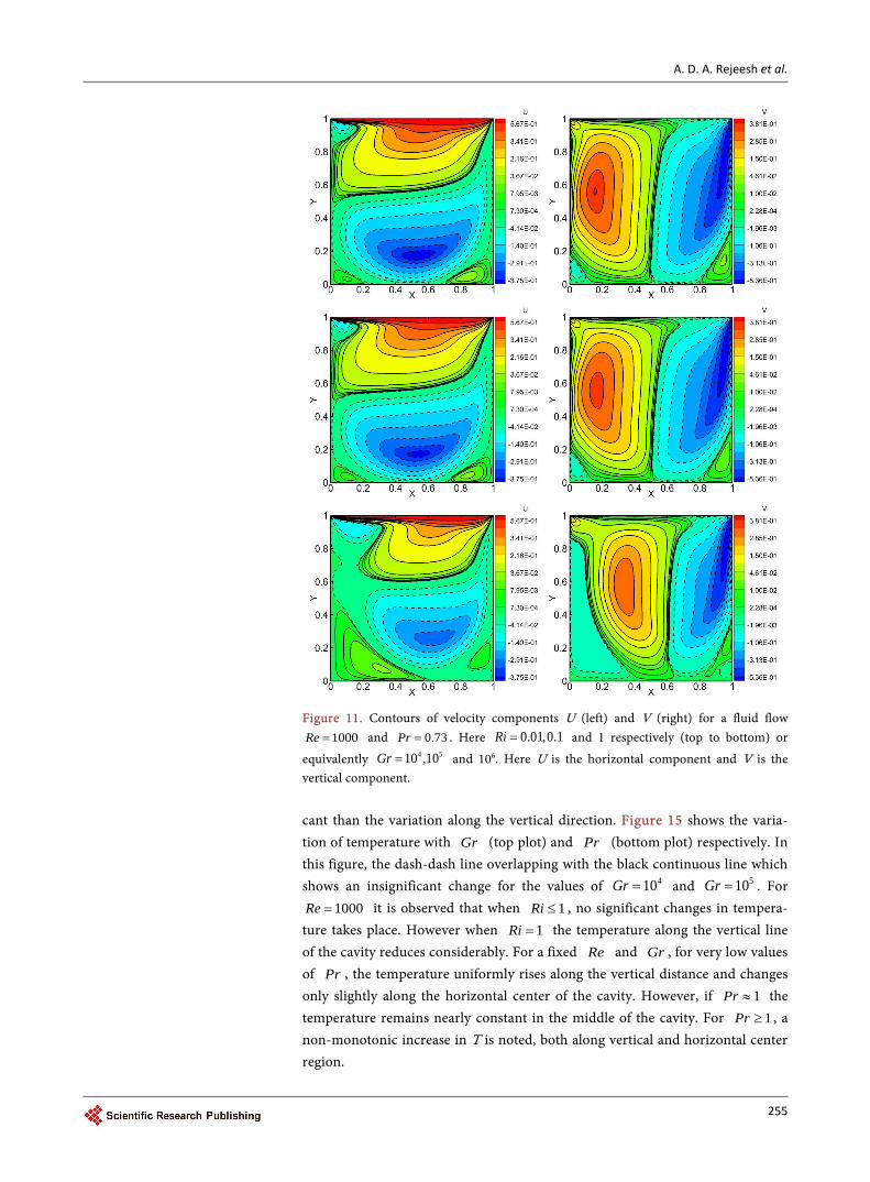
410Gr = . bottom left of Figure 4. For the case of 1000Re = (Figure 11) however, the minimal viscous force causes the formation of multiple recirculation region. It is also noted that, both velocity components are responsible for the emergence of corner vortices. While increasing Re the growth of secondary vortices are visi-ble to both velocity components, this effects are due to the conventional flows in a lid-driven cavity. Also the contour lines are pushed towards the top region of the cavity. Due to the push of buoyant force against the gravity, USE grows and finally it form a separate cell near the bottom region of the cavity in the hori-zontal velocity component, which is visible in the Figure 11 (bottom left). It is also noted that the horizontal components of velocity undergoes changes as high as three orders of magnitude within the cavity.

Cross sectional profiles of velocity and temperature Figure 12 shows the ver-tical (v) and horizontal (u) components of velocities along the x and y directions

252

A. D. A. Rejeesh et al.

Figure 9. For a fairly large buoyancy force 1Ri = , the effect of Pr on the streamlines (left) and temperature isotherms (right) for the flow of fluid with 1000Re = are shown. Here 0.015Pr = , 0.73 and 7 respectively (top to bottom). Equivalent Grashof number is

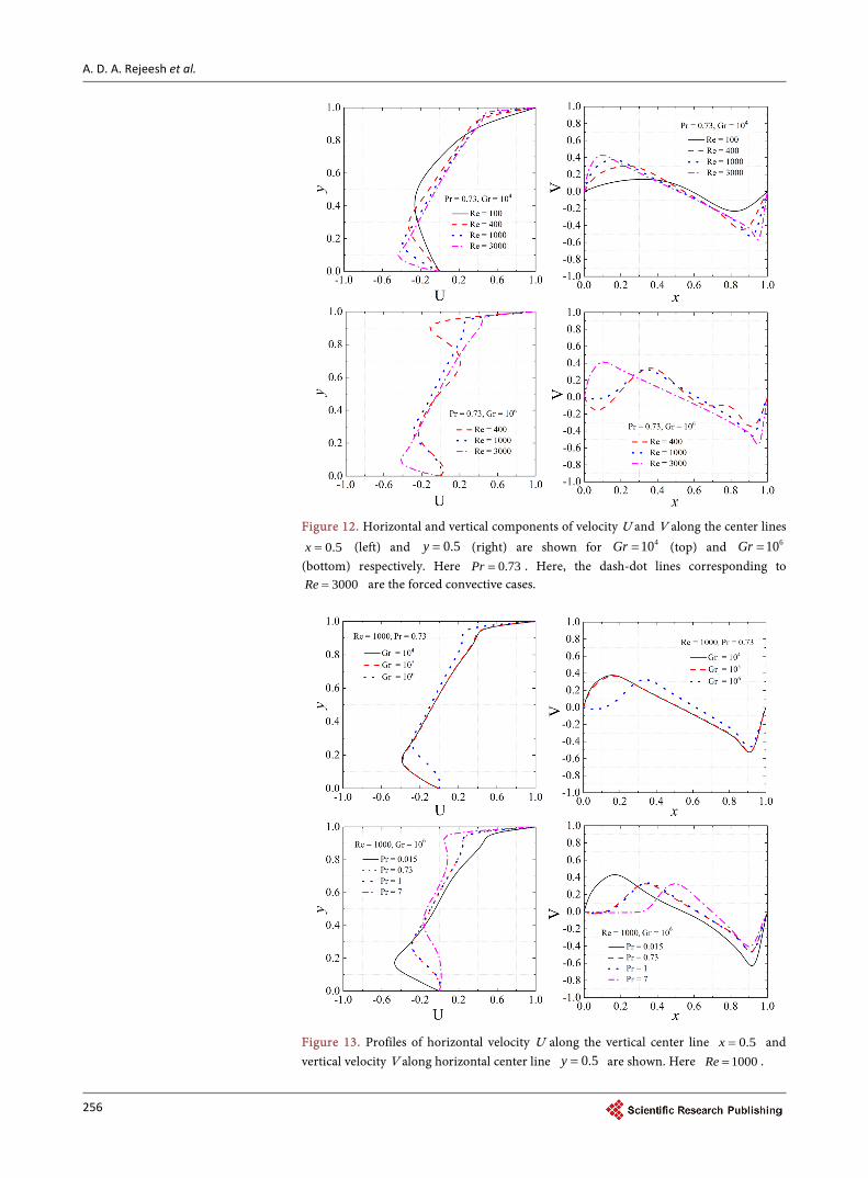
610Gr = . along vertical center line and horizontal mid-heights respectively. The dash-dot lines of Figure 12 show the flow in forced convective range. In this case, the ve-locity is maximum near the walls and the fluid is stagnant in center region of the cavity. This is the expected behavior of lid-driven cavity flow in the absence of buoyant force. In other cases, the velocity changes considerably. Figure 13 shows the variation of velocity with Gr (top plot) and Pr (bottom plot) re-spectively. From the top plot it is clear that while increasing buoyancy effect the fluid tends to degrade the shear action by moving the line closely towards the stagnant line. Prandtl number have vital effect to pull the fluid to stagnant which is visible from the bottom plot. Figure 14 shows the temperature profile along vertical and horizontal directions at horizontal mid-length and vertical mid- height for different values of Gr and Re respectively. All curves shows

253

A. D. A. Rejeesh et al.

Figure 10. Contours of velocity components U (left) and V (right) for 0.01,1Ri = and 10 respectively (top to bottom) for a flow of fluid with 100Re = and 0.73Pr = . Equivalent values of Gr are 102, 104 and 105 respectively from top to bottom. Here U is the horizontal component and V is the vertical component. minimum temperature at bottom wall and maximum at top wall. In the case of

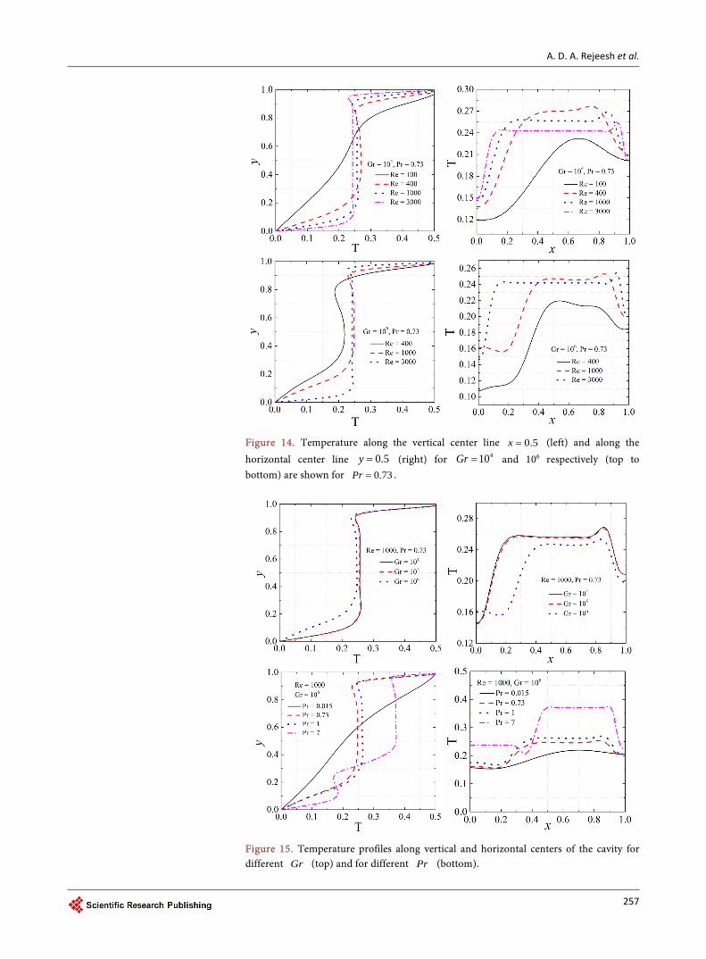
1Ri (continuous line plot), for a fixed Re , temperature distribution shows a linear variation along vertical direction due to the fact that the fluid inside the cavity is almost stagnant which is seen in the Figure 14 (top left, 100Re = ). Hence the gradient of temperature is pronounced. Same variation is observed along the horizontal direction Figure 14 (top right, 100Re = ). In the shear force dominated case 1Ri , the temperature variation is significant only very near to the walls, where the conductive heat transfer is dominant and in the middle portion of the cavity, temperature change is insignificant due to the re-circulation of fluid, where the convective heat transfer is dominant. The bottom plots in the same Figure 14 shows the case of different Grashof number ( 610Gr = ). In this case the horizontal variation of temperature is more signifi-

254

A. D. A. Rejeesh et al.

Figure 11. Contours of velocity components U (left) and V (right) for a fluid flow

1000Re = and 0.73Pr = . Here 0.01,0.1Ri = and 1 respectively (top to bottom) or

equivalently 4 510 ,10Gr = and 106. Here U is the horizontal component and V is the vertical component. cant than the variation along the vertical direction. Figure 15 shows the varia-tion of temperature with Gr (top plot) and Pr (bottom plot) respectively. In this figure, the dash-dash line overlapping with the black continuous line which shows an insignificant change for the values of 410Gr = and 510Gr = . For

1000Re = it is observed that when 1Ri ≤ , no significant changes in tempera-ture takes place. However when 1Ri = the temperature along the vertical line of the cavity reduces considerably. For a fixed Re and Gr , for very low values of Pr , the temperature uniformly rises along the vertical distance and changes only slightly along the horizontal center of the cavity. However, if 1Pr ≈ the temperature remains nearly constant in the middle of the cavity. For 1Pr ≥ , a non-monotonic increase in T is noted, both along vertical and horizontal center region.

255

A. D. A. Rejeesh et al.

Figure 12. Horizontal and vertical components of velocity U and V along the center lines

0.5x = (left) and 0.5y = (right) are shown for 410Gr = (top) and 610Gr = (bottom) respectively. Here 0.73Pr = . Here, the dash-dot lines corresponding to

3000Re = are the forced convective cases.

Figure 13. Profiles of horizontal velocity U along the vertical center line 0.5x = and vertical velocity V along horizontal center line 0.5y = are shown. Here 1000Re = .

256

A. D. A. Rejeesh et al.

Figure 14. Temperature along the vertical center line 0.5x = (left) and along the horizontal center line 0.5y = (right) for 410Gr = and 106 respectively (top to bottom) are shown for 0.73Pr = .

Figure 15. Temperature profiles along vertical and horizontal centers of the cavity for different Gr (top) and for different Pr (bottom).

257

A. D. A. Rejeesh et al.

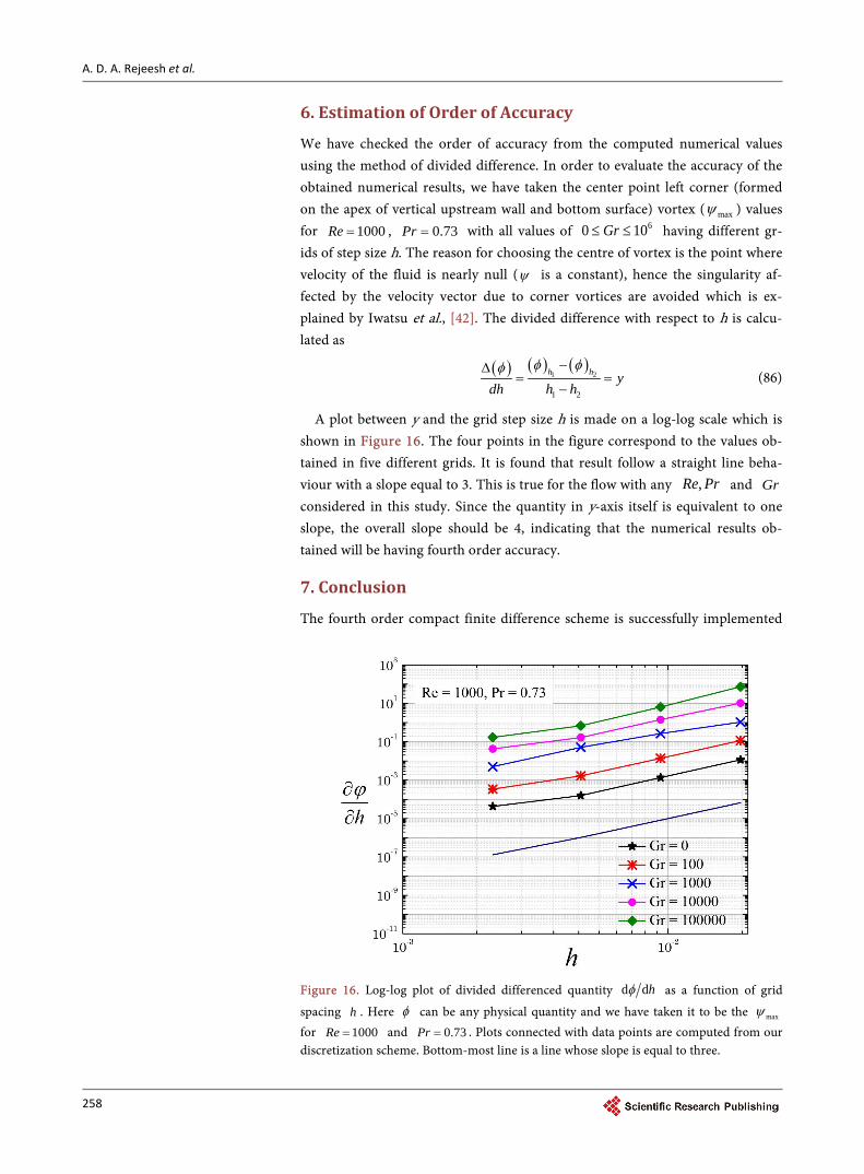
6. Estimation of Order of Accuracy

We have checked the order of accuracy from the computed numerical values using the method of divided difference. In order to evaluate the accuracy of the obtained numerical results, we have taken the center point left corner (formed on the apex of vertical upstream wall and bottom surface) vortex ( maxψ ) values for 1000Re = , 0.73Pr = with all values of 60 10Gr≤ ≤ having different gr-ids of step size h. The reason for choosing the centre of vortex is the point where velocity of the fluid is nearly null (ψ is a constant), hence the singularity af-fected by the velocity vector due to corner vortices are avoided which is ex-plained by Iwatsu et al., [42]. The divided difference with respect to h is calcu-lated as

( ) ( ) ( )1 2

1 2

h h ydh h h

φ φφ −∆= =

− (86)

A plot between y and the grid step size h is made on a log-log scale which is shown in Figure 16. The four points in the figure correspond to the values ob-tained in five different grids. It is found that result follow a straight line beha-viour with a slope equal to 3. This is true for the flow with any ,Re Pr and Gr considered in this study. Since the quantity in y-axis itself is equivalent to one slope, the overall slope should be 4, indicating that the numerical results ob-tained will be having fourth order accuracy.

7. Conclusion

The fourth order compact finite difference scheme is successfully implemented

Figure 16. Log-log plot of divided differenced quantity d dhφ as a function of grid

spacing h . Here φ can be any physical quantity and we have taken it to be the maxψ for 1000Re = and 0.73Pr = . Plots connected with data points are computed from our discretization scheme. Bottom-most line is a line whose slope is equal to three.

258

A. D. A. Rejeesh et al.

To study the mixed convection in a lid driven cavity flow with linearly heated top wall. The multigrid iterative procedure allowed a fast convergence to the ex-act solution. The effect of heat transfer is affected by all the governing parame-ters as well as the effect of linear heating. The growth and the degradation of USE and DSE are observed for the increase of Richardson number, which shows a significant effect of Ri over heat transfer. In the mixed convection range, the USE and DSE are merging. The velocity contour shows that, both velocity com-ponents are responsible for the emergence of corner vortices. For 1Ri ≥ , a push of buoyant force against the gravity occurs and hence the USE grows and finally it forms a separate cell near the bottom region of the cavity in the horizontal ve-locity component. The order of accuracy of the derived numerical scheme is found to be four.

Acknowledgements

One of the authors (R. Sivakumar) would like to thank the UGC for supporting this research work through major project grant vide UGC project grant letter F. No. 37-312/2009 (SR) dated January 12, 2010, and also DST for infrastructure development funds through FIST program vide order SR/FST/PSII-021/2009 dated August 13, 2010. A. D. Abin. Rejeesh acknowledges the DST-INSPIRE fel-lowship vide DST/INSPIRE/Fellowship/2011/361 order dated August 01, 2013 and finally S. Udhayakumar acknowledges Pondicherry University for providing scholarship.

References [1] Ghia, U. and Ghia, K.N. and Shin, C.T. (1982) High-Re Solution for Incompressible

Flow Usingg the Navier-Stokes Equations and a Multigrid Method. Journal of Computational Physics, 48, 13-15.

[2] Cha, C.K. and Jaluria, Y. (1984) Recirculating Mixed Convection Flow for Energy Extraction. International Journal of Heat and Mass Transfer, 27, 1801-1812.

[3] Hsu, T.H. and Hsu, P.T. and How, S.P. (1997) Mixed Convection in a partially Di-vided Rectrangular Enclosure. Numerical Heat Transfer, Part A: Applications, 31, 655-683. https://doi.org/10.1080/10407789708914058

[4] Hsu, T.H. and Wang, S.G. (2000) Mixed Convection in a Rectrangular Enclosure with Discrete Heat Sources. Numerical Heat Transfer, Part A: Applications, 38, 627-652. https://doi.org/10.1080/104077800750021170

[5] Fedorov, A.G. and Visakanta, R. (2000) Three-Dimensional Conjugate Heat Trans-fer in the Microchannel Heat Sink for Electronic Packaging. International Journal of Heat and Mass Transfer, 43, 399-415.

[6] Leong, C.W. and Ottono, J.M. (1989) Experiments on Mixing Due to Chaotic Ad-vection in a Cavity. Journal of Fluid Mechanics, 209, 463-499. https://doi.org/10.1017/S0022112089003186

[7] Alleborn, N. and Rasziller, H. (1999) Lid-Driven Cavity with Heat and Mass Transport. International Journal of Heat and Mass Transfer, 42, 833-853.

[8] Imberger, J. (1982) Dynamics of Lakes, Reservoirs and Cooling Ponds. Annual Re-view of Fluid Mechanics, 14, 153-187. https://doi.org/10.1146/annurev.fl.14.010182.001101

259

A. D. A. Rejeesh et al.

[9] Prasad, A.K. and Koseff, J.R. (1996) Combined Forced and Mixed Convection Heat Transfer in a Deep Lid-Driven Cavity Flow. International Journal of Heat and Fluid Flow, 17, 460-467.

[10] Elsherbiny, S.M. (1996) Free Convection in Inclined Air layers Heated from Above. International Journal of Heat and Mass Transfer, 39, 3925-3930.

[11] Prasad, Y.S. and Das, M.K. (2007) Hopt Bifurcation in Mixed Convection Flow in-side a Rectangular Cavity. International Journal of Heat and Mass Transfer, 50, 3583-3598.

[12] Basak, T., Roy, S., Sharma, P.K. and Pop, I. (2009) Analysis of Mixed Convection Flows within a Square Cavity with Uniform and Non-Uniform Heating of Bottom Wall. International Journal of Thermal Sciences, 48, 891-912.

[13] Cheng, T.S. and Liu, W.H. (2010) Effect of Temperature Gradient Orientation on the Characteristics of Mixed Convection Flow in a Lid-Driven Square Cavity. Computers and Fluids, 39, 965-978.

[14] Erturk, E. and Gokol, C. (2006) Fourth Order Compact Formulation of Navier- Stokes Equations and Driven Cavity Flow at High Reynolds Numbers. Numerical Methods in Fluids, 50, 421-436.

[15] Cheng, T.S. (2011) Characteristics of Mixed Convection Heat Transfer in a Lid-Driven Square Cavity with Various Richardson and Prandtl Numbers. Interna-tional Journal of Thermal Sciences, 50, 197-205.

[16] Ahmed, S.E., Oztop, H.F. and Al-Salem, K. (2016) Effects of Magnetic Field and Viscous Dissipation on Entropy Generation of Mixed Convection in Porous Lid-Driven Cavity with Corner Heater. International Journal of Numerical Methods for Heat and Fluid Flow, 26, 1548-1566. https://doi.org/10.1108/HFF-11-2014-0344

[17] Malleswaran, A. and Sivasankaran, S. (2016) A Numerical Simulation on MHD Mixed Convection in a Lid-Driven Cavity with Corner Heaters. Journal of Applied Fluid Mechanics, 9, 311-319. https://doi.org/10.18869/acadpub.jafm.68.224.22903

[18] Kareem, A.K., Gao, S. and Ahmed, A.Q. (2016) Unsteady Simulations of Mixed Convection Heat Transfer in a 3D Closed Lid-Driven Cavity. International Journal of Heat and Mass Transfer, 100, 121-130.

[19] Bettaibi, S., Sediki, E., Kuznik, F. and Succi, S. (2015) Lattice Boltzmann Simulation of Mixed Convection Heat Transfer in a Driven Cavity with Non-Uniform Heating of the Bottom Wall. Communications in Theoretical Physics, 63, 91-100. https://doi.org/10.1088/0253-6102/63/1/15

[20] Hussein, I.Y. and Ali, L.F. (2014) Mixed Convection in a Square Cavity Filled with Porous Medium with Bottom Wall Periodic Boundary Condition. Journal of Engi-neering, 20, 99-119.

[21] Ismael, M.A., Pop, I. and Chamkha, A.J. (2014) Mixed Convection in a Lid-Driven Cavity with Partial Slip. International Journal of Thermal Sciences, 82, 47-61.

[22] Mahapatra, T.R., Pal, D. and Mondal, S. (2013) Effects of Buoyancy Ratio on Double-Diffusive Natural Convection in a Lid-Driven Cavity. International Journal of Heat and Mass Transfer, 57, 771-785.

[23] Mekroussi, S., Nehari, D., Bouzit, M. and Chemloul, N.E.S. (2013) Analysis of Mixed Convection in an Inclined Lid-Driven Cavity with a Wavy Wall. Journal of Mechanical Science and Technology, 27, 2181-2190. https://doi.org/10.1007/s12206-013-0533-9

[24] Al-Salem, K., Oztop, H.F., Pop, I. and Varol, Y. (2012) Effects of Moving Lid Direc-tion on MHD Mixed Convection in a Linearly Heated Cavity. International Journal of Heat and Mass Transfer, 55, 1103-1112.

260

A. D. A. Rejeesh et al.

[25] Basak, T., Pradeep, P.V.K., Roy, S. and Pop, I. (2011) Finite Element Based Heatline Approach to Study Mixed Convection in a Porous Square Cavity with Various Wall Thermal Boundary Conditions. International Journal of Heat and Mass Transfer, 54, 1706-1727.

[26] Mamourian, M., Shirvan, K.M. and Rahimi, R.E.A.B. (2016) Optimization of Mixed Convection Heat Transfer with Entropy Generation in a Wavy Surface Square Lid-Driven Cavity by means of Taguchi Approach. International Journal of Heat and Mass Transfer, 102, 544-554.

[27] Nayak, R.K., Bhattacharyya, S. and Pop, I. (2016) Numerical Study of Mixed Con-vection and Entropy Generation of Cu-Water Nanofluid in a Differentially Heated Skewed Enclosure. International Journal of Heat and Mass Transfer, 85, 620-634.

[28] Kefayati, G.H.R. (2015) FDLBM Simulation of Mixed Convection in a Lid-Driven Cavity Filled with Non-Newtonian Nanofluid in the Presence of Magnetic Field. International Journal of Thermal Sciences, 95, 29-46.

[29] Kefayati, G.H.R. (2014) Mixed Convection of Non-Newtonian Nanofluid in a Lid-Driven Enclosure with Sinusoidal Temperature Profile using FDLBM. Powder Technology, 256, 268-281.

[30] Jamai, H., Fakhreddine, S.O. and Sammouda, H. (2014) Numerical Study of Sinu-soidal Temperature in Magneto-Convection. Journal of Applied Fluid Mechanics, 3, 493-502.

[31] Kefayati, G.H.R., Bandpy, M.G., Sajjadi, H. and Ganji, D.D. (2012) Lattice Boltzmann Simulation of MHD Mixed Convection in Lid-Driven Square Cavity with Linearly Heated Wall. Scientia Iranica, 19, 1053-1065.

[32] Arani, A.A.A., Sebdani, S.M., Mahmoodi, M., Ardeshiri, A. and Aliakbari, M. (2012) Numerical Study of Mixed Convection Flow in a Lid-Driven Cavity with Si-nusoidal on Sidewalls Using Nanofluid. Superlattices and Microstructures, 51, 893- 911.

[33] Nasrin, R. (2010) Mixed Magnetoconvection in a Lid-Driven Cavity with a Sinu-soidal Wavy Wall and a Central Heat Conducting Body. Journal of Naval Architec-ture and Marine Engineering, 7, 13-24. https://doi.org/10.3329/jname.v8i1.6793

[34] Karimipour, A., Efse, M.H., Safaei, M.R., Semiromi, D.T., Jafari, S. and Kazi, S.N. (2014) Mixed Convection of Copper-Water Nanofluid in a Shallow Inclined Lid Driven Cavity Using the Lattice Boltzmann Method. Physica A: Statistical Mechan-ics and Its Applications, 402, 150-168.

[35] Chamkha, A.J. and Abu-Nada, E. (2012) Mixed Convection Flow in Single- and Double-Lid Driven Square Cavities Filled with Water-Al2O3 Nanofluid: Effect of Viscosity Models. European Journal of Mechanics B-Fluids, 36, 82-96.

[36] Garoosi, F. and Rashidi, M.M. (2015) Two Phase Simulation of Natural Convection and Mixed Convection of the Nanofluid in a Square Cavity. Powder Technology, 275, 239-256.

[37] Billah, M.M., Rahman, M.M., Sharif, U.M., Rahim, N.A., Sadidur, R. and Hasanuz-zaman, M. (2011) Numerical Analysis of Fluid Flow Due to Mixed Convection in a Lid-Driven Cavity Having a Heated Circular Hollow Cylinder. International Com-munications in Heat and Mass Transfer, 38, 1093-1103.

[38] Wesseling, P. (1982) Theoretical and Practical Aspects of a Multigrid Method. SIAM Journal on Scientific and Statistical Computing, 3, 387-407. https://doi.org/10.1137/0903025

[39] Zhang, J. (2003) Numerical Simulation of 2D Square Driven Cavity Using Fourth Order Compact Finite Difference Scheme. Computers and Mathematics with Ap-plications, 45, 43-52.

261

A. D. A. Rejeesh et al.

[40] Botella, O. and Peyret, R. (1998) Benchmark Spectral Results on the Lid-Driven Cavity Flow. Computers and Fluids, 27, 421-433.

[41] Bruneau, C.H. and Saad, M. (1998) The 2D Lid-Driven Cavity Problem Revised. Computers and Fluids, 35, 326-348.

[42] Iwatsu, R., Hyun, J.M. and Kuwamura, K. (1993) Mixed Convection in a Driven Cavity with a Stable Vertical Temperature Gradient. International Journal of Heat and Mass Transfer, 36, 1601-1608.

[43] Sharif, M.A.R. (2007) Laminar Mixed Convection in Shallwl Inclined Driven Cavi-ties with Hot Moving Lid on Top and Cooled from Bottom. Applied Thermal En-gineering, 27, 1036-1042.

[44] Koseff, J.R. and Street, R.L. (1984) Visualization Studies of a Shear Driven Three-Dimensional Re-Circulating Flow. Journal of Fluids Engineering, 106, 21-29. https://doi.org/10.1115/1.3242393

[45] Koseff, J.R. and Street, R.L. (1984) The Lid-Driven Cavity Flow: A Synthesis of Qua-litative and Quantitative Observations. Journal of Fluids Engineering, 106, 390-398. https://doi.org/10.1115/1.3243136

[46] Moallemi, M.K. and Jang, K.S. (1992) Prandtl Number Effects on Laminar Mixed Convection Heat Transfer in a Lid-Driven Cavity. International Journal of Heat and Mass Transfer, 35, 1881-1892.

[47] Torrance, K., Davis, R., Eike, K., Gill, P., Gutman, D., Hsui, A., Lyons, S. and Zien, H. (1972) Cavity Flows Driven by Buoyancy and Shear. Journal of Fluid Mechanics, 51, 221-213. https://doi.org/10.1017/S0022112072001181

[48] Schreiber, R. (1983) Driven Cavity Flows by Efficient Numerical Techniques. Jour-nal of Computational Physics, 49, 310-333.

Submit or recommend next manuscript to SCIRP and we will provide best service for you:

Accepting pre-submission inquiries through Email, Facebook, LinkedIn, Twitter, etc. A wide selection of journals (inclusive of 9 subjects, more than 200 journals) Providing 24-hour high-quality service User-friendly online submission system Fair and swift peer-review system Efficient typesetting and proofreading procedure Display of the result of downloads and visits, as well as the number of cited articles Maximum dissemination of your research work

Submit your manuscript at: http://papersubmission.scirp.org/ Or contact ojfd@scirp.org

262