Mittag-Leffler Distributions and Long-Run

Behavior of Some Macroeconomic Models

Masanao Aoki∗

Department of EconomicsUniversity of California, Los Angeles

Fax Number 310-825-9528, e-mail aoki@econ.ucla.edu

May,2006

Abstract

This paper discusses long-run behavior of economic models with many in-teracting heterogeneous agents, and point out the connection with the classof Mittag-Leffler distributions.

In the process, the paper summarizes some known asymptotic propertiesof a class of one- and two-parameter Poisson-Dirichlet distribution models,and those of the model discussed by Feng and Hoppe. These models havealso known long-run behavior after some suitably normalized numbers ofpartitions and the components of partition vectors, such as non-vanishingvariances of cluster sizes as the number of agents becomes large. Some dif-ferences in the long-run behavior between the class of one-parameter modelsand that with two-parameters are pointed out. Convergence behavior is ex-pressed in terms of generalized Mittag-Leffler distributions in the statisticsliterature. We exhibit power laws when they exist as well.

Second, a numerical example of a model which is outside the frameworkof one- and two-parameter Poisson Dirichlet models mentioned above. Thismodel has more than two parameters but is a simple model composed oftwo types of agents, innovators and immitators. This model has non-selfaveraging variaces and the covariance of the sizes of the two sectors, thatis the variances and the covariance do not vanish as the number of agentsapproach infinity.

Key Words:Two-parameterPoisson-Dirichlet distributions; Mittag-Lefflerdistributions; nom-self averaging phenomena, Power laws.

∗The author is grateful for many helps he received from M. Sibuya. Ted Theodosopou-los and an anonymous referee’s comments are useful in revising the original draft. I thankthem all. The simulation was run by G. Yoshida and K. Ono, Department of Physics,Chuo University, Tokyo.

1

Introduction

In old industrial organization literature, several tests and measures of degreeof industrial concentration have been used to to decide if a given industryis monopolistic or not. See for example Scherer (1980) for various casestudies. One such test is called Herfindahl, or Herfindahl-Hirschman indexof concentration. It is defined as the sum of squares of fractions of shares,i.e.,

H =∑

i

x2i ,

where xi is the fraction of ”share” of markets or sales by sector i or firmi. By definition xi is positive, and sum to one,

∑i xi = 1. As we discuss

shortly, this literasture used a rudimentary version of the size-biased sam-pling scheme as a test for oligopoly. This meassure of concentration is usedin both domestic and foregin trade context. It is sometimes (mistakenly)called Gini-index.1

The question of concentration is that of distribution of fractions of thenumbers of clusters, and the numbers of agents by types. A simple ap-plication of shares of market by two types of agents, using one-parameterPoisson-Dirichlet distribution (also called Ewens distribution, Ewens (1972,1979, 1990)) has been made by Aoki (2000a, 2000b).

This paper develops further the original ideas in these papers by applyingsome of the results from two-parameter Poisson-Dirichlet distributions inthe recent combinatorial stochastic process literature, by Kingman (1993),Carlton (1999), Holst (2001), Pitman (1999, 2002), and his associates.

In physics literature, Mekjian and Chase (1997) have used two-parametermodels. They refer to the work by Pitman (1996). There are other works inthe physics literature, in particular the papers by Derrida-Flyvbjerg men-tioned in footnote 1, and Derrida (1994a, 1997).2 There are other papersin the physics literature that deal with random partitions. Higgs (1995)have noted the similarities of some physical distributions and power laws,and mention population genetics papers by Ewens in particular. Frontera,Goicoechea, Rafols, and Vivies (1995), and Krapivsky, Grosse, and BenNadin (2002) discuss partitions and fragmentations, that is, stick-breadingversion of the residual allocation processes explicitly. They have not touchon connections with the two-parameter Poisson-Dirichlet distributions.

In macroeconomic and finance modelings, agents of different character-istics or strategies are of different types and form separate clusters andaffect aggregate behavior. In this paper, we therfore explore more broadlyeconomic implications of long-run relations that may exist among non-selfaveraging economic or financial variables.

1Sometimes it is called Gini-Simpson index of divesity. See Hirschman (1960) aboutthe origin and mis-attribution of this notion to Herfindahl. In the population geneticsliterature H is called homozygosity. See Ewens (1972). Interestingly, the same measure hasbeen used by Derrida-Flyvbjerk (1989) in discussing relative sizes of basins of attractions ofKaufman random maps and ramdom dynamics in statistics and physics. These, however,involve a sigle parameter θ in their statistical description. See also Aldous (1985).

2Derrida (1994b) has added some material on residual allocation models.

2

In the first part of this paper we introduce the reader to some basicnotions on random partitions from the literature of combinatorial stochasticprocesses, in particular the works by statisticians, J. Pitman (1996, 2002)and Yamato and Sibuya (2000). Size-biased permutation, residual allocationmodels, notions of frequency spectrum and structure distribution, Mittag-Leffler probability density and power-laws are introduced in the process ofdescribint long-run behavior of models.

We show, among other things, that components of partition vectors inPD(α, θ) with positive α have non-vanishing variances (non-self averagingin the physics terminology), while in PD(θ) they do not.

Invariance under Size-biased Permutation

We introduce the notion of invariance under size-biazed sampling or permu-tation in the statistics literature as a proper concepts of distribution of sizesof types in statisstical equilibrium.

Heuristically this notion may arise in the following way: Suppose thatfractions of ”shares” are arranged in decreasing order, x1 > x2 > · · ·. Wemay be interested in the question of how large is the share of the secondtype, excluding the presence of the first, that is the largest type. This isthe fraction x2/(1 − x1). Analogously, we may be interested in the i-thlargest type excluding or correcting for the effects of the first through the(i − 1)th shares, given by xi/(1 − x1 − · · ·xi−1). Actually, this is one ofthe ways industrial organizaation economists measured the concentration ofindustries, even though they did not know of the notion of the size-biasedsampling or permutation. This is precisely what is involved in size-biasedsampling.

More formally, we consider the set of all possible fractions (p1, p2, . . .)where pi, the fraction of type i agents, is posistive, and the fractions sum to1,∑

i pi = 1. Suppose that one agent is sampled. The probability that thefirst sampled agent is of type j is

Pr(p1 = pj |p1, p2, . . . , pn) = pj , : j = 1, 2, . . .n.

This first pick is called the size-biased pick, because types of agents withlarger fraction are most likely to be sampled. This equation says that thesample is taken in proportion to the sizes of various types. More generally,having picked p1, . . . , pk, the next sampled agent is of type n with probabilitygiven by

Pr(pk+1 = pn|pi, i = 1, 2, . . . , k; p1, p2, . . .) =pn

1 − p1 − p2 − · · · − pk,

provided that pn 6= pi, i = 1, 2, . . . , k. The collection, {pj}, is called size-biased sampling or permutation abbreviated as SBP.

Since distributions of agents by types are more useful when they are instatistical equilibrium, we define the set of fractions is invariant under sizebiased permutation (abbreviated as ISBP) when

{pn} =d {pn},

3

where =d means equality in distribution.Pitman (1996) considered {pn}, pn > 0, a.s., for all n,

∑n pn = 1, such

that {pn} are distributed as RAM (residual allocation model) for indepen-dent random variables Wi, i = 1, 2, . . ., that is ps are generated by thefollowing formula

p1 = W1, p2 = W2(1−W1), · · · , pn = Wn(1 −W1)(1−W2) · · ·(1 −Wn−1).

Note that p1 = W1, p2/(1− p1) = W2, · · · , pn/(1− p1 −· · ·− pn−1) = Wn

are independent.Let α and θ be such that 0 ≤ α < 1, and θ > −α > 0. Let Wi be Beta

distriuted random variable, Be(1−α, θ+ iα), where random variable X hasdensity Be(a, b) when the density is given by

fX(x) =1

B(a, b)xa−1(1− x)b−1,

for 0 < x < 1, where B(a, b) = Γ(a)Γ(b)/Γ(a+ b).Then {pn} is said to have a GEM(α, θ) distribution.3 With α = 0, the

above reduces to the one-parameter Poisson-Dirichlet distribution, due toKingman (1978). See Perman, Pitman, and Yor (1992), and Pitman andYor (1997) on earlier works.

Then he showed that {pn} is invariant under size-biased permutation,abbreviated as ISBP, if and only if {pn} is distributed as GEM(α, θ).

Next, arrange samples by order statistics, i.e., we reorder pi, i = 1, 2, . . .as

p(1) > p(2) > · · · .

When {pn} is distributed as GEM(α, θ), then the ranked sequence {p(n)}is said to have the two-parameter Poisson Dirichlet distribution, PD(α, θ).

To summarize, if fractions of agents of type n is given by {pn}, pn > 0,a.s., and

∑n pn = 1, the size-biased permutation of PD(α, θ) is aGEM(α, θ),

and the ranked sequence of a GEM(α, θ) is a PD(α, θ). Furthermore,GEM(α, θ) is ISBP. See Carlton (1999), for example.

With α = 0, PD(α, θ) reduces to the Ewens distribution, denoted fromnow on by PD(θ).

Structural Distribution and Frequency Spectrum

The structural distribution, F , of {pn}, is defined by Engen to be the dis-tribution on (0, 1] of the first size-biased pick, that is the first term of asize-biased permutation of the distribution of agents by type, {pn}, that isp1. The importance of this first pick is demonstrated by the lemma belowof Pitman and Yor (1997).

When {pn} is distriubted as a two parameter Poisson-Dirichlet distribu-tion PD(α, θ), let W1 be distributed as Be(1−α, θ+α) (Beta distribution).We drop subscript 1 from W1 from now on. The first size-biased pick is

3The name GEM was given by Ewens to honor the pioneers, Griffiths, Engen, andMcCloskey.

4

p1 = W as we have shown above. The structural distribution is importantbecause it shows that p1 summarizes the distribution of {pn} as shown next.

Lemma: For any positive measureable function g(t) ∼ O(t) as t goes tozero,

E[g(W )/W ] = E[g(p1/p1]

= E{E∑

i

g(pn)pn

Pr(p1 = pn|p1, p2, . . .)}

= E(∑ g(pn)

pnpn) = E[

∑g(pn)].

Pitman (1996) pointed out that v−1F (dv) is the frequency spectrum. Bythe above lemma, the expected value of any positive measurable function gis expressible in terms of the structural distribution as

E(∑

n

g(pn)) =∫ 1

0

g(v)vF (dv).

If one takes g to be I(a < v < b), this expression gives the average number ofn such that a < pn < b, hence v−1F (dv) is the same as the frequency spec-trum in population genetics literature. In that literature, there is a measureof cluster size distribution called frequency spectrum. See Ewens (1979).Aoki (2002, p.173, 2002a) has some elementary economic applications ofthis notion. In words, the frequency spectrum is the expected number oftypes with fraction in the interval (x, x+ dx).

Given order statistics of cluster sizes governed by PD(θ), x1 > x2 > · · ·,the largest size x1 has the density

f(x1) = θx−11 (1 − x1)θ−1,

for x1 in the range 1/2 < x1 < 1, that is when the largest cluster is morethan 1/2 of the whole.4 This density behaves like x−1

1 for small x1. Thisindicates that there are many types with small fractions and f(x) is notnormalizable. However, g(x) = xf(x) = θ(1 − x)θ−1 is normalizable. Thisfunction is interpreted as the probability that a randomly selected sampleis of the type with fraction in (x, x+ dx).

The two largest fractions, x1 and x2 have the joint density

f(x1, x2) = θ2(x1x2)−1(1− x1 − x2)θ−1,

when the two sizes are such that 0 < x1 + x2 < 1, and more importantlywhen

x2

1 − x1>

12.

Note that similar inequalities arise in size-biased permutation. See Aoki(2002, Sec. 10.6) for heuristic derivations based on Watterson and Guess(1977). 5

4The expression is more complicated when x1 is less than 1/2. See Watterson andGuess (1977).

5Karlin (1967) focussed on the situation with many types of small probabilities suchthat β(x) = x−γL(x), with 0 < γ < 1, and where β(x) =

∑∞i

I(pn ≥ x), and where L(.)is some slowly varying function.

5

In economic applications we are more interested in a few types with largeshares, such as the ones discussed in Aoki (2000a).

For the one-parameter Poisson-Dirichlet process, the expected sizes ofthe three largest clusters are shown in the next table (see Griffiths (2005))

θ largest second third

0.1 0.935 .059 .005

0.5 .758 .171 .049

1.0 .624 .210 .088

For example, with θ = 0.1, the expected size of the largest and the secondlargest clusters sum to 99 per cent of the whole agents. With θ = 1/2, thesum is about 93 per cent.

Number of Clusters in two-parameter Poisson-Dirichlet

Distributions

The probabilities of new types entering models in PD(θ), and the num-ber of clusters have been applied for example in Aoki (2002, p.176, App.A.5). In the two-parameter Poisson-Dirichlet distribution the conditionalprobabilities for the number of clusters in a sample of size n, Kn is given by

Pr(Kn+1 = k + 1|K1, . . . , Kn = k) =kα+ θ

n + θ, (1)

andPr(Kn+1 = k|K1, . . . , Kn = k) =

n− kα

n+ θ. (2)

In other words, the random variable Kn is the number of different typesof agents present in a sample of size n. Eq.(1) means that the (n + 1)thentrant is a new type. Eq.(2) means that it is one of the previously existingtypes. Hence the number of clusters does not change.

From (1) and (2) the probability for Kn = k, q(n, k), can be recursivelycomputed using the conditional probability equation above

q(n+ 1, k) =(n− kα)(n+ θ)

q(n, k) +θ + (k − 1)α

n+ θq(n, k − 1), (3)

for 1 ≤ k ≤ n, given the boundary formula

q(n, 1) =(1 − α)(2 − α) · · ·(n− α)(θ + 1)(θ + 2) · · ·(θ + n)

,

andq(n, n) =

(θ + α)(θ + 2α) · · ·(θ + nα)(θ + 1)(θ + 1 + α) · · ·(θ + 1 + α(n − 1))

.

6

These expressions generalize the recurrence relation for the one-parameterPD(θ). In the one-parameter case, θ/(θ+n) is a probability that the (n+1)thagent that enter the model is a new type, and n/(θ + n) is the probabilitythat the next agent is one of the types already in the model.

In the one-parameter case, qn,k := P (Kn = k) is governed by the recur-rence relation

qn+1,k =n

n+ θqn,k +

θ

θ + nqn,k−1.

The solution of this recurrence equation is expressible as

qn,k =c(n, k)θk

θ[n],

where θ[n] := θ(θ + 1) · · ·(θ + n − 1) = Γ(θ+n)Γ(θ) , and c(n, i) is the unsigned

(signless) Stirling number of the first kind. It satisfies the recursion

c(n+ 1, k) = nc(n, k) + c(n, k− 1).

Since qn,k sums to one with respect to k we have

θ[n] =n∑

k=1

c(n, k)θk. (4)

See Aoki (2002, p.208) for example on the Stirling numbers, and theircombinatorial interpretations. In the two-parameter PD(α, θ) case, theprobability of the number of clusters is given by

Pα,θ(Kn = k) =θ[k,α]

αkθ[n]c(n, k;α), (5)

whereθ[k,α] := θ(θ + α)(θ + 2α) · · ·(θ + (k − 1)α),

and the expression c(n, k;α) generalizes the signless Stirling number of thefirst kind of one-parameter situation.

Let Sα(n, k) := 1αk c(n, k;α). It satisfies the recursion

Sα(n+ 1, k) = (n− kα)Sα(n, k) + Sα(n, k − 1).

This is called generalized Stirling number of the first kind. See Char-alambides (2002). Instead of (4) we have

θ[n] =n∑

k=1

Sα(n, k)θ[k,θ]. (6)

Pitman (1999) obtained its asymptotic expression as

Sα ∼ Γ(n)Γ(k)

n−αα1−kgα(x),

where k ∼ xnα. Here, gα is the Mittag-Leffler function. This function isdiscussed in the next section.

7

Asymptotic Behavior of Cluster Sizes

We collect here some known facts about cluster sizes as n→ ∞.

The number of clusters Kn

Yamato and Sibuya (2000) obained

EKn =θ

α[(θ + α)[n]

θ[n]− 1],

where we note that

(θ + α)[n]

θ[n]=

Γ(θ)Γ(θ + α)

Γ(θ + α+ n)Γ(θ + n)

.

Applying the asymptotic expression for the Gamma function for large n

Γ(n + a)Γ(n)

∼ na,

to the above expression, we have an asymptotic expression,

E(Kn

nα) ∼ Γ(θ + 1)

αΓ(θ + α). (7)

They also calculate the asymptotic value of the variance of Kn/nα,

var(Kn/nα) ∼ Γ(θ + 1)

α2γα,θ ≥ 0, (8)

whereγα,θ :=

θ + α

Γ(θ + 2α)− Γ(θ + 1)

[Γ(θ + α)]2. (9)

Note thatFact: γ0,θ = 0.This fact is important in the long-run behavior of components of the

partition vectors, to be discussed in the next subsection.Actually they calculate more generally

limE(Kn

nα)r = µ′r ,

where µ′r is the r− th moment of the generalized Mittag-Leffler distributionwith density

gα,θ :=Γ(θ + 1)

Γ(θ/α + 1)x

θα gα(x),

where θ/α > −1, and where gα(x) is the Mittag-Leffler (α) density func-tion. It is known that this function is uniquely determined by the momentconditions ∫ ∞

0xpgα(x)dx =

Γ(p+ 1)Γ(pα+ 1)

,

for all p > −1. Note that the integral of gα,θ over the interval from zero toinfinity is 1, as it should be.

See also Blumenfeld and Mandelbrot (1997) who credit Feller (1949) asthe original source.

8

Mittag-Leffler distributions

As we discuss more fully later, Pitman (2002, Sec. 3) has stronger result:

Kn/nα → L, a.s.,

where the expression L has the density

d

dsPα,θ(L ∈ ds) = gα,θ

where letting η = θα we define

gα,θ(s) :=Γ(θ + 1)Γ(η + 1)

sγgα(s),

where s > 0, and where gα = gα,0 is the Mittag-Leffler density

gα(s) =1π

∞∑

k=1

[Γ(kα)Γ(k)

sin(kπα)(−s)k−1].

We note that

µ′1 = Eα,θ(L) = Γ(θ + 1)/αΓ(θ + α),

andµ′2 = Eα,θ(L2) = Γ(θ + 1)(θ + α)/α2Γ(θ + 2α).

Hence variance of L is given as µ′2 − (µ′1)2.

For the record we have

varα,θ{Kn

nα} = varα,θL.

The partition vector a

Denote the partition vector by a = (a1, a2, . . .), where we recall that ai isthe number of distinct clusters of size i, hence

∑i ai = Kn, and

∑i iai = n.

Yamato and Sibuya obtain the limit of the first component, a1

limE[a1

nα] =

Γ(θ + 1)Γ(θ + α)

,

andlim var(

a1

nα) = Γ(θ + 1)γα,θ ≥ 0.

In fact aj/nα are all non-self averaging, as well as jaj/n

α, where jaj isthe total number of agents in the clusters of size j. Note that their variancesare all zero with α = 0, that is the asymptotic variance of aj/n

α are all zeroin PD(θ) models.

FactThe expression ai/n

α, i ≥ 1 are all non-self averaging.

9

Sibuya (2005) used Formula 6.1.41 in Abramovitz and Stegun (1965) toobtain asymptotic expression

E(aj

nα) ≈ (1− α)[j−1]

j!Γ(θ + 1Γ(θ + α)

+O(n−1).

We state this asProposition: As in (9)

lim varα,θ(Kn/nα) = varα,θ(L),

andlim varα,θ(aj/n

α) = α2varα,θ(L).

They also show that covariances of components of the partition vectorsare non-self averaging with positive α values:

limCov(ai

nα,aj

nα) = Γ(θ + 1)γα,θ ×

(1 − α)[i−1]

i!(1− α)[j−1]

j!> 0, : α > 0.

It is also known that

j!Γ(1− α)αΓ(j − α)

→d L. (10)

We have

E(aj

nα|kn = k) ∼ (1 − α)[j−1]

j!(1 − j/n)−(1+α) × ξ,

where ξ depends on g(α,θ).The number of clusters, Kn is spread among the components of the

partition vector, ai, i = 1, 2, . . . , n at the proportion α(1 − α)[j−1]/j!, 0 <α < 1. Devroye (1993) calls this Sibuya distribution.

We also note that

LimE(ai)E(Kn

=α2

Γ(θ + α)γα,θ.

We note that aj/Kn is self-averaging for all j = 1, . . . , n. Yamato andSibuya also examined the clusters of size k or less

K[1, k] := a1 + a2 + · · ·+ ak,

and the number of agents in K[1, k], denoted by N [1, k] and obtained theirlimiting expressions as

K[1, k]nα

→d {1− (1− α)[k]

k!}L,

and

N [1, k]nα

→d α(2 − α)[k−1]

(k − 1)!L,

10

Sibuya also notes that

{ a1

nα,2a2

nα· · · .kak

nα}

converges in distribution to a sequence of random variables depending on Las

{1, (1 − α)1!

, · · · , (1− α)[k−1]

(k − 1)!}.

In PD(α) it is known that

Kn − θlnn√θlnn

→ N(0, 1).

Hence (Kn/lnn) is self-averaging.

Almost sure convergence

Denote by aj(n) the number of clusters of size j when there are n agents inthe model. We noted earlier that

∑nj=1 jaj(n) = n, and Kn :=

∑nj aj(n) is

the total number of clusters formed by the total of n agents.By Rouault (1976, 1978)

aj(n)Kn

→ αΓ(j − α)Γ(1 − α)j!

, a.s.

Recallint that Kn/nα → L,a.s., we have

aj(n)/nα → αΓ(j − α)Γ(1 − α)j!

L, a.s.

wbereaj(n)Kn

→ α

j!Pα,j ,

wherePαj =

Γ(j − α)Γ(1 − α)

,

for every j = 1, 2, . . . a.s. as n goes to infinity, and that aj(n) ∼ Pα,jLnα

in a two-parameter Poisson-Dirichlet case.

Local Limit Theorem

Suppose N independent positive random variables Xi, i = 1, 2, . . .N arenormalized by their sum SN = X1 + · · ·+XN

xi = Xi/SN , i = 1, . . .N,

so thatY1 :=

∑

i

xi = 1.

11

Suppose that the probability density ofXi is such that it has a power-lawtail,

ρ(x) ∼ Ax−1−µ,

with 0 < µ < 1. Then, SN/N1/µ has a stable distribution (called Levy

distribution).Pitman’s formula for the probability of Kn = k, with k ∼ snα indicates

that the power law nα which is 2α < 2 or 2α = 1 + µ with 0 < µ < 1, thecase in Derrida.

With the 2-parameter PD distribution satisfying the power law condi-tion, Derrida’s conclusion that the Hs are non-self averaging applies to thiscase as well.

Estimating the Parameters

Carlton (1999) and Sibuya (2005)are the only systematic source on estimat-ing the parameters of two-parameter Poisson-Dirichlet distributions.

With α = 0, Ewens had shown that Kn is the sufficient statistics for θ.Carlton discusses the case where α is known and θ unknown. He derivesthe asymptotic distribution of the maximum likelihood estimate of θ, givenn samples.

LemmaGiven α in (0,1), the maximum-likelihood estimate of θ, θn is given by

ψ(1 + θn/α) − αψ(1 + θn) → logS, as.

Here ψ is the digamma function.With θ known, and α unknown, Carlton provesLemmaLet {A1, . . . , An} is distributed according to the two-parameter Ewens

distribution of size n. (His Eq. (4.2) on page 55.) Then,

αn =logKn

logn→ α a.s.

Sibuya uses the conditional probability distribution of the partition vec-tor components, given that

∑i ai = k, and expresses the distribution

P (a|∑

aj = k) =1

Sα(n, k)n!∏aj !

∏

j

{(1− α)[j−1]

j!}aj

which is proportional to

exp{−∑ j

2(j − 2)!aj}α+ O(α2)

and test the hypothesis α = 0, against the alternative hypothesis α < 0.He proposes the rejection region

∑ j

2(j − 2)!− aj > const.k.

When both parameters are unknown, the estimation problem is appar-ently unsolved.

12

Some Potential Applications

In physics literature, Derrida (1994 a, b)sketched a derivation that the ex-pected values of Yk =

∑i x

ki , k = 2, 3, . . . can be calculated for mean field

spin glass models using the Parisi replica approach, and remarkably theformula is the same as the GEM model described above.

In the rest of this section we focus on economic examples.Example 1 Scaling of GDP growth rates was considered by Canning,

Amaral, Lee, Meyer, and Stanley (1998). They showed that the standarddeviation of the GDP growth rate may sclae as Y −β , with β about 0.15.Here, we heuristically explain how their finding may be explained using arandom partition framework.

We modify the model of Huang and Solomon (2001) and apply the sameprocedures to estimate the growth rate of real GDP.6 View the real economyas composed of K sectors of various sizes. Stochastically one or more of thesectors experience what we call elementary events, the aggregate of whichyields the real growth of the economy, leading to its random growth rates. Tobe simple one may assume that the individual elementary growth of sectorsis random λ = 1+g, where g = ±γ randomly with some positive γ. Further,we adopt the mechanism of Huang and Solomon that a random number τof this type of elementary events are experienced in a unit of calendar time.The random growth rate is the composite effects of these random elementaryevents.

We refer the detail of the mechanism to their paper, and mention onlythat the growth rate will be exponential only if the number of changes τ isless than some critical value τc, and change in GDP has a power law densitywith index −(1 + α).

The value of α is defined to be the ratio of minimum and average realconsumption in the model q = cmin/caverage, and is tied to α by

α ≈ 1/(1− q),

when K is sufficiently larger that e1/q, due to inherent normalization condi-tions of densities involved.

For example, setting q = 0.25 leads to α = 1.33, and K must be suchthat K >> e4 > 55. The value of τc is defined by (N/2q)α. With τ less thanτc, the growth rate r can be shown to have the density

p(r) = Cexp(−a|r − rm|),

for r > rm, with a different constant for the case r < rm.The deviation of r is then related to variability ofK and τ , among others.

From this one can deduce that the average deviation in the growth rates isbasically determined by percentage changes of the size of the largest clusterwhich can be related to the GDP when the productivity is assumed not tovary too much, and the conclusion follows that the standard deviation of

6Their focus is on financial sector, not real sector. See Aoki and Yoshikawa (2006 a,b).

13

the growth rate is Y −µ with µ less than 1. See Aoki and Yoshikawa (2006a,b) for detail.

Example 2: Long-run effects of innovation and imitationThis example is based on a two-sector model discussed in Aoki (2002,

Sec. 7.4), Aoki, Nakano, Yoshida (2004), and Aoki, Nakano, and Ono (2006).There are two types of firms, innovators and imitators.

Our model has two sectors; one technically advanced sector and the otherless so. By a suitable choice of units we denote the sizes of the two sectorsby a vector (n1, n2). We may think of them as the number of firms in somesuitably chosen standard units. Firms in sector one succeed in creatinginnovative firms at rate f which is, for simplicity, exogenously fixed in thismodel.7

Firms’ stochastic behavior is described by a continuous time Markovchain which is uniquely determined by a set of transition rates. We write thetransition rate from state a to b by w(a, b). This means that the probabilitythat the system moves from state a to b in some small time interval is givenby the time interval times the transition rates up to o(time interval size).They are specified as follows: The first two describe entry (growth) rates

w{(n1, n2), (n1 + 1, n2)} = c1n1 + f,

w{(n1, n2), (n1, n2 + 1)} = c2n2.

Here ci is the rate of growth of type i firm size, i = 1, 2.The next two specify exit rates from the model

w{(n1, n2), (n1 − 1, n2)} = d1n1,

w{(n1, n2), (n1, n2 − 1)} = d2n2.

Here di is the exit (death) rate of type i firms from the economy, i = 1, 2.The last set of two transition rates describes how firms change their types

w{(n1, n2), (n1 + 1, n2 − 1)} = µg1n2(n1 + h),

with g2 = c2/d2, and h = f/c1, and

w{(n1, n2), (n1 − 1, n2 + 1)} = µg2n1n2,

with gi = ci/di, i = 1, 2, and µ = λd1d2. This parameter λ is the coefficientin the transition rates of type changes by firms in the two sectors. The firstof the two shows the rate at which one of type 1 firm becomes technologicallyobsolete and join the cluster made up of type 2 firms. The second equationspecifies how firms of type 2 successfully imitate firms of type 1 and jointheir cluster. for example.

With these transition rates, we write the master equation. We computethe probability generating function, and then convert it into the cumulantgenerating function, since we are interested in calculating only the first andsecond order moments, k1, k2, k1,1, k1,2, and k2,2, and verify that the 2× 2

7It will be interesting to endogenize this rate in a way that is not equivalent to increasingthe birth rate c1 in the model of this section.

14

covariance matrix is positive definite in steady state. Fortunately, this modelis specified in such a way that the equations for the moment are closed at thesecond moments, that is no higher order moments appear in the equationsfor the first and second moments. We derive a coupled ordinary differentialequations for these moments. With the help of Mathematica we calculatethe stationary state values of these moments for varioous parameter values,and verify the positive definiteness of the second moment matrix.

To the knowledge of the author this is the first example of Schumpert-erian dynamics with innovations and immitation effects for which the firsttwo moments have been analytically derived and numerically evaluated. Themodel allows us to examine parametrically the relative importance of netdeath rate and innovation rate, and draw conclusions about qualitative be-havior of interacting two sectors. The model shows that both sectors co-existin the long-run. We show also that the means of stationary locally stableequilibria scale with parameters of the innovation rate, and death rate.

The stochastic dynamic equation is easy to state. It is a backwardChapman-Kolmogorov equation, also known as the master equation. (Weuse the latter name as it is short, and implies that everything you need toknow about stochastic behavior is implicit in the master equation.)

∂P (n1, n2; t)∂t

= I(n1, n2; t) −O(n1, n2; t), (11)

where the first term collects all inflows of probability flux into state (n1, n2),and the second term collects all outflows of probability fluxes out of thisstate. There are six distinct flows. In detail we have

I(n1, n2; t) = P (n1 + 1, n2; t)d1(n1 + 1) + P (n1, n2 + 1; t)d2(n2 + 1)

+P (n1 − 1, n2; t)c1(n1 − 1 + h) + P (n1, n2 − 1)c2(n2 − 1)

+P (n1+1, n2−1; t)µg2(n1+1)(n2−1)+P (n1−1, n2+1; t)µg1(n1−1+h)(n2+1).

The second term in (1) is given by

O(n1, n2; t) = P (n1, n2; t){c1+n1+f+c2n2+d1n1+d2n2+µg1n2(n1+h)+µg2n1n2)}.

To solve the master equation, we first convert it into the probabilitygenerating function

G(z1, z2; t) =∑

n1 ,n2

P (n1, n2; t)zn11 zn2

2 .

We obtain a partial differential equation for G(z1, z2; t). It is given inAppendix. This partial differential equation is rather intractable, and forthat reason we convert it into the cumulant generating function and solvefor the expected values of first and second moments.8

Cumulant generating functions are related to the probability generatingfunctions by

K(θ1, θ2; t) = lnG(e−θ1 , e−θ2),8In some cases the resulting ordinary differential equations for the moments turn out

to be an infinite set of coupled ordinary differential equation. Fortunately, the differentialequations for the first and second cumulants are self-contained in this model.

15

where we change variables from z1, and z2 into θ1 and θ2.It is known that the cumulant generating function has a Taylor series

expansion of the form

K(θ1, θ2; t) = k1θ1 + k2θ2 +12(θ1, θ2)Θ(θ1, θ2)′ + · · · ,

where k1 = E(n1), and k2 = E(n2), that is, they are the expected sizes ofthe two types, and where Θ is a covariance matrix made up of the variancesand covariances of the two sizes,

Θ =

(k1,1 k1,2

k1,2 k2,2

).

See Aoki (2002, Chapt. 7) for further information on these generatingfunctions, and some simple examples.

From the cumulant generating functions we derive a set of five ordinarydifferential equations for k1, k2, k1,1, k1,2, and k2,2.

Appendix gives the explicit expressions.

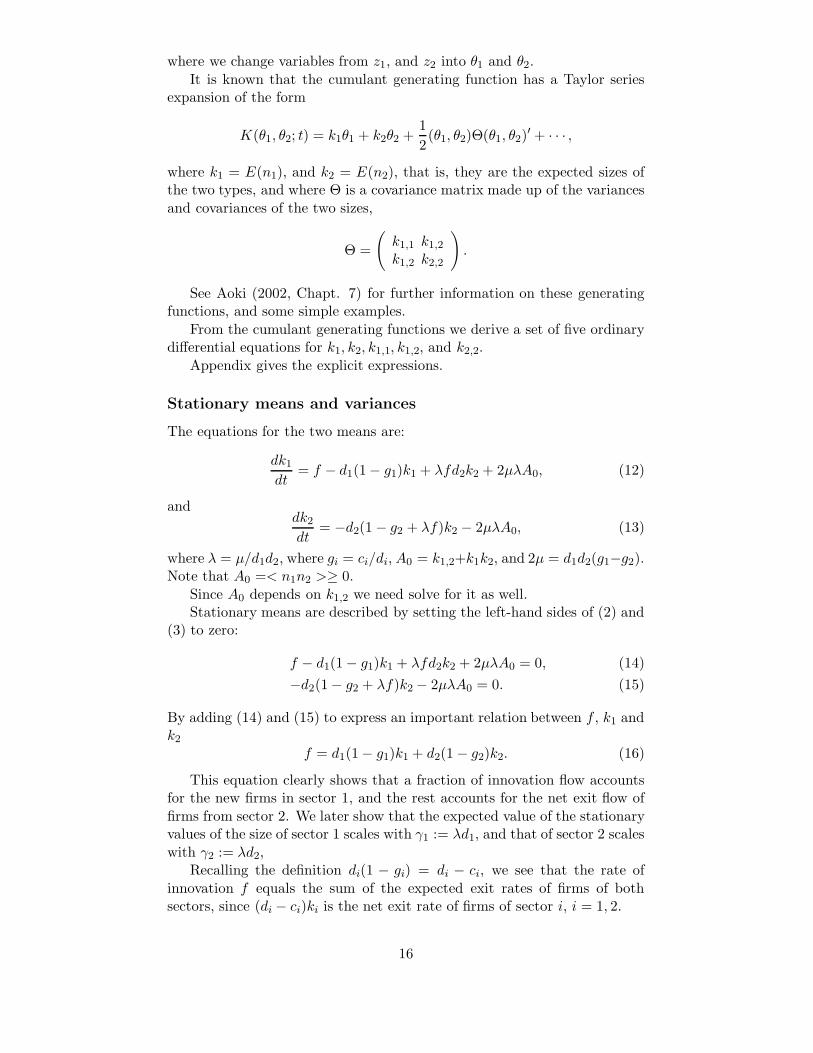
Stationary means and variances

The equations for the two means are:

dk1

dt= f − d1(1− g1)k1 + λfd2k2 + 2µλA0, (12)

anddk2

dt= −d2(1 − g2 + λf)k2 − 2µλA0, (13)

where λ = µ/d1d2, where gi = ci/di,A0 = k1,2+k1k2, and 2µ = d1d2(g1−g2).Note that A0 =< n1n2 >≥ 0.

Since A0 depends on k1,2 we need solve for it as well.Stationary means are described by setting the left-hand sides of (2) and

(3) to zero:

f − d1(1− g1)k1 + λfd2k2 + 2µλA0 = 0, (14)−d2(1− g2 + λf)k2 − 2µλA0 = 0. (15)

By adding (14) and (15) to express an important relation between f , k1 andk2

f = d1(1− g1)k1 + d2(1 − g2)k2. (16)

This equation clearly shows that a fraction of innovation flow accountsfor the new firms in sector 1, and the rest accounts for the net exit flow offirms from sector 2. We later show that the expected value of the stationaryvalues of the size of sector 1 scales with γ1 := λd1, and that of sector 2 scaleswith γ2 := λd2,

Recalling the definition di(1 − gi) = di − ci, we see that the rate ofinnovation f equals the sum of the expected exit rates of firms of bothsectors, since (di − ci)ki is the net exit rate of firms of sector i, i = 1, 2.

16

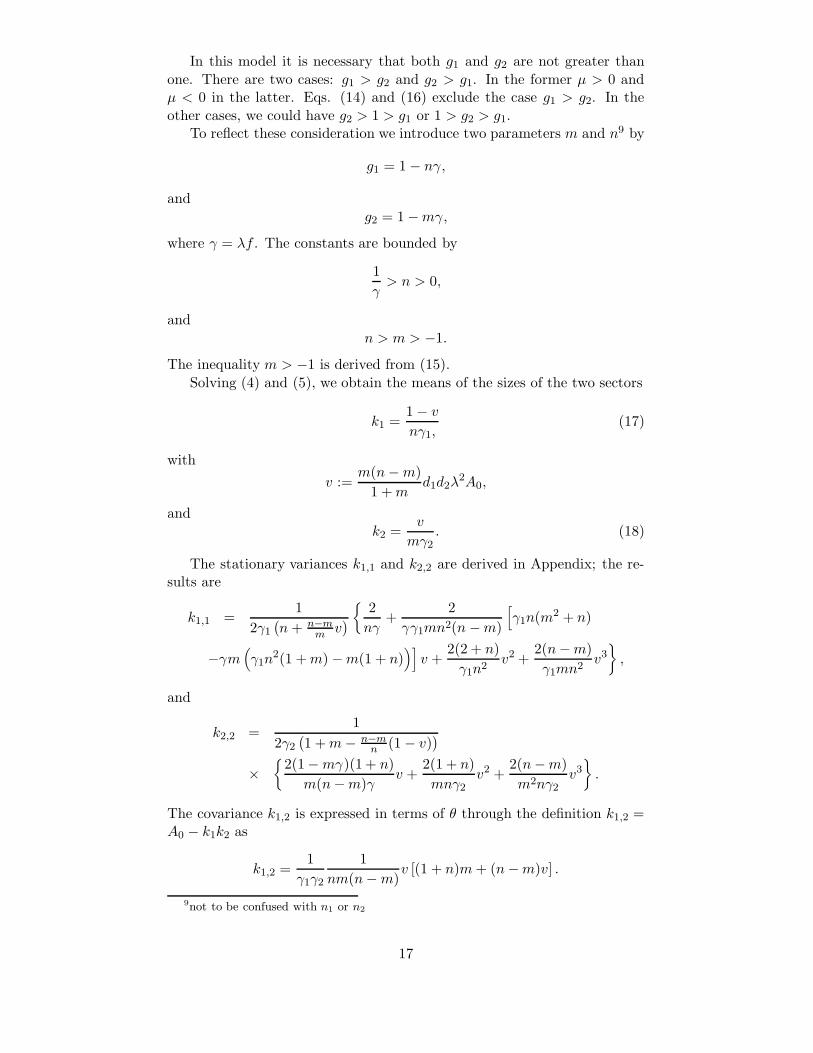
In this model it is necessary that both g1 and g2 are not greater thanone. There are two cases: g1 > g2 and g2 > g1. In the former µ > 0 andµ < 0 in the latter. Eqs. (14) and (16) exclude the case g1 > g2. In theother cases, we could have g2 > 1 > g1 or 1 > g2 > g1.

To reflect these consideration we introduce two parameters m and n9 by

g1 = 1 − nγ,

andg2 = 1 −mγ,

where γ = λf . The constants are bounded by

1γ> n > 0,

andn > m > −1.

The inequality m > −1 is derived from (15).Solving (4) and (5), we obtain the means of the sizes of the two sectors

k1 =1 − v

nγ1,(17)

withv :=

m(n−m)1 +m

d1d2λ2A0,

andk2 =

v

mγ2. (18)

The stationary variances k1,1 and k2,2 are derived in Appendix; the re-sults are

k1,1 =1

2γ1

(n + n−m

m v){

2nγ

+2

γγ1mn2(n −m)

[γ1n(m2 + n)

−γm(γ1n

2(1 +m) −m(1 + n))]v +

2(2 + n)γ1n2

v2 +2(n−m)γ1mn2

v3},

and

k2,2 =1

2γ2

(1 +m− n−m

n (1 − v))

×{

2(1−mγ)(1 + n)m(n−m)γ

v +2(1 + n)mnγ2

v2 +2(n−m)m2nγ2

v3}.

The covariance k1,2 is expressed in terms of θ through the definition k1,2 =A0 − k1k2 as

k1,2 =1

γ1γ2

1nm(n−m)

v [(1 + n)m+ (n−m)v] .

9not to be confused with n1 or n2

17

What remains is to determine v. The self-consistent equation for v isderived in Appendix. Although the equation is a fifth order equation of vbecause of the five unknown quantities, the highest term vanishes so that

vF (v) = 0 (19)

whereF (θ) = r0 + r1v + r2v

2 + r3v3. (20)

The forms of ri are given in Appendix.The root θ = 0 is of interest because this value of θ yields a stationary

state in which sector 2 vanishes, k2 = 0, k2,2 = 0, and k12 = 0.Hence we have the solutions for (19); solutions of F (v) = 0 in addition

to v = 0. For v = 0 one has

k1 =1nγ1

, k11 =1

n2γγ1, k2 = k22 = k12 = 0,

which corresponds to the situation that only sector 1 survives. From F (v) =0 we obtain three values of v The roots must be such that v is real and theobtained values of k1, k2, k1,1 and k2,2 are positive; k1,2 is not necessarilypositive. Although the analytic solutions may be obtained for special set ofparameters, such solutions are not possible in general.

Mathematica, however, enables us to numerically solve F (v) = 0. Inorder that those solutions exist in reality, the solutions must be the stablefixed points.

As an example we describe in detail the case where m = .01; n = 2,γ = γ1, and γ2 = γ1 + ε, with a small positive ε. In this case there is onlyone root for which the dynamics are locally stable. It is given by v = 0.472.

The stability of the stationary states is examined in the following way.The starting equations are (12), (13) and (21), (22) and (23) in Appendix.By setting the left hand sides of those equations we have the stationaryvalues, which are confirmed to numerically coincide with the solutions fromvF (v) = 0. Then the linearized equations for deviations δk1, δk2, δk11, δk22

and δk12 from the stationary values are derived. The eigenvalues of thoseequations are numerically calculated with a help of Mathematica. If realparts of all five eigenvalues associated with a stationary point are negative,the stationary point is stable.

The value of v = .472 corresponds to a locally stable solution. This leadsto

k1 =.264γ1

, k2 =47.2γ2

.

From (5) we obtain

A0 =v

γ1γ2

1 +m

m(n−m)=

23.956γ1γ2

.

From this we derive

k1,2 = A0 − k1k2 =11.495γ1γ2

.

18

From (9) through (11) we can obtain approximate order of magnitude valuesfor the second moments k1,1 and k2,2 as follows.

k1,1 =C1,1

γ21

,

withC1,1 ≈ 1

n2(1 + v2) ≈ .31,

which is close to .309 obtained in the numerical example below, and

k2,2 =C2,2

γ22

,

withC2,2 ≈ 1

m2[v2 +

m(1 + n)n

v] = 2300.

We also have an approximate expression for k12 as C12/γ1γ2 with

C12 =θ2

mn≈ 11.15,

which is in good agreement with the value obtained above as 11.495.

Numerical Examples

We focus on a stationary solutions. Since there are five parameters, we havemany solutions.

To keep the sizes of the two sectors at reasonable values, we examinecases with the death rates close to the birth rates. Namely, we choose gi tobe close to unity. Previously we have indicated that g2 can be either largerthan one or smaller than one, while g1 is always less than one. First, weconsider the case that the death rate di is slightly larger than the birth rateci, so that nγ, mγ � 1. Although the death rate of sector 2 is consideredto be larger than that of sector 1, we assume that both are almost thesame. We focus on the following parameters; γ = γ1 = γ2 = 0.01, n =2.0, m = 0.01. Then we have three types of solutions; (1) k1 = 50, k11 =2500, k2 = k22 = k12 = 0, (2) k1 = 49.97, k2 = 4.77, k11 = 2501, k22 =46505, k12 = 3.71 and (3) k1 = 26.4, k2 = 4719, k11 = 3093, k22 = 2.37 ×107, k12 = 114918. The stable solution is only the first type; only sector1 survives. The second and third types are not stable. If we increase γ2

slightly to γ2 = 0.011, a remarkable change occurs in the type 3 solution.The numbers for (1) are the same as the previous case. On the other hand,(2) k1 = 49.977, k2 = 4.122, k1,1 = 2501, k2,2 = 40232, k1,2 = 3.2 and (3)k1 = 23.94, k2 = 4738, k1,1 = 3216.7, k2,2 = 2.378 × 107, k1,2 = 127042. Thesecond solution is not stable, but the third solution turns out to be stablein this case.

We vary a value of γ2 with other parameters fixed. We found that thestable fixed point exists in a narrow range such that 0.02>∼γ2>∼0.0102.

What parameters are chosen to increase the number of companies? Forthat purpose we should decrease γ, γ1, γ2. When n = 2.0 and m = 0.01

19

are fixed, we employ γ = γ1 = 0.001, γ2 = 0.0011. Then we have thestable third solution k1 = 264, k2 = 47193 with the correlation coefficientk1,2/

√k1,1k2,2 = 0.42. In other sets of parameters with n and m fixed at

the above values, γ = γ1 and γ2 being slightly larger than γ, we have thefollowing scaling relation

k1 =0.264γ1

, k2 =47.2γ2

, k1,1 =0.309γ2

, k2,2 =2374γ2

, k1,2 =11.5γ2

.

The correlation coefficient is 0.42.The coefficient of variations are 2.11 and 1.03 for the two sectors respec-

tively. We also note that with γ2 nearly the same as γ1 only 0.6 percent ofthe total sizes of the capital resides in sector 1.

Next we examine negative values of m. Take m = −0.01 while keepingthe values of the other parameters the same as before. The numerical calcu-lation gives a negative value of k2. Although we have not done an extensivestudy, a negative value of m, i.e., g2 is larger than one, may not yield stablestationary situations.

Aoki, Nakano, and Ono (2006) has more extensive simulations and verifynon-self averaging property for the stationary sizes of the two sectors.

Example3: Disequilibrium theory of long run profits. Iwai’smodel has more than two sectors with different productivity coefficients.His paper is too long and involved to give a thumb-nail sketch here. Insteadwe offer three quotes from his paper to explain what he does.

...while both the differential growth rates among different efficiencyfirms and the diffusion of better technologies through imitations pushthe state of technology towards uniformity, the punctuated appearanceof technological innovations disrupts this equilibrating tendency.

... over a long passsage of time these conflicting microscopic forceswill balance each other in a statistical sense and give rise to a long-rundistribution of relative efficiencies across firms. This long-run distribu-tion will in turn allow us to deduce an upward-sloping long-run supplycurves...

This paper has challenged this long-held tradition in economics. Ithas introduced a simple evolutionary model which is capable of analyz-ing the development of the industry’s state of technology as a dynamicinterplay among many a firm’s growth, imitation and innovation activ-ities. And it has demonstrated that what the industry will approachover a long passage of time is not a classical or neoclassical equilib-rium of uniform technology but a statistical equilibrium of technolog-ical disequilibria which maintains a relative dispersion of efficienciesin a statistically balanced form. Positive profits willl never disappearfrom the economy nomatter how long it is run. ’Disequilibrium’ theoryof ’long-run profits’ is by no means a condtradition in terms.

We see that our random partiton framework along the line of Aoki,Nakano, and Yoshida (2004) can be applied to at least three types of firms,and their tail distribution may satisfy power laws to substantiate Iwai’sclaim by using long-run in time rather than the thermodynamic limits.

20

Concluding Remarks

In physics non-self-averaging phenomena abound. In traditional microe-conomic foundations of economics, one deals almost exclusively with well-posed optimization problems for the representative agents with well definedpeaks and valleys of the cost functions. It is also taken for granted thatas the number of agents goes to infinity, any unpleasant fluctuations vanishand well defined deterministic macroeconomic relations prevail. In otherwords, non-self-averaging phenomena are not in the mental pictures of av-erage macro- or microeconomists.

However, we know that as we go to problems which require agents tosolve some combinatorial optimization problems, this nice picture may dis-appear. In the limit of the number of agents going to infinity some resultsare sample-dependent and deterministic results will not follow. Some of thistype of phenomena have been reported in Aoki (1996, Sec. 7.1.7) and also inAoki (1996, p. 225) where Derrida’s random energy model was introduced tothe economic audience. Unfortunately it did not catch the attention of theeconomic audiences. See Mertens (2000) for a simple example, or Krpisvskyet al (2000). This paper is another attempt at exposing non-self-averagingphenomena in economics, in particular in problems involving combinatorialoptimization. We also have mentioned a possibility of extending the phraseto cover existence of non-degenerate distributions with time going to infinity.What are the implications if some economic models have non-self averagingproperty? For one thing, it means that we cannot blindly try for larger sizesamples in the hope that we obtain better estimates.

The example above is just an indication of the potential of this approachof using exchangeable random partition methods. It is the opinion of thisauthor that subjects such as in the papers by Fabritiis, Pammolli, and Ric-caboni (2003), or by Amaral et al (1998) could be re-examined from therandom combinatorial partition approach with profit. Another example isSutton (2002). He modeled independent business in which the business sizesvary by partitions of integers to discuss the dependence of variances of firmgrowth rates. He assumed each partition is equally likely, however. Useof random partitions discussed in this paper may provide more realistic orflexible framework for the question he examined. It would be an interest-ing application of the random partition theory and see if non-self-averagingphenomena exist in the sense of physics literture in this area.

References

Aldous, D.J., (1985), ”Exchangeability and related topics” in Lecture notesin mathemaatics, No.1117, Springer-Verlarg, Berlin

Amaral, Luis A. Nunes, S. V. Buldyrev, S. Havlin, M.A. Salinger andH.E. Stanley,(1998) ”Power law scaling for a system of interacting units withcomplex internal structure, Phys. Rev. Lett,80, 1385–1388.

Aoki, M., and H. Yoshikawa (2002). ”Demand saturation-creation andeconomic growth ” J. Econ. Behav. Org.,48, 127-154. Aoki, M., ( 2000a),”Open models of share markets with two dominant types of participants, ”,

21

J.Econ. Behav. Org.49 199-216.—-, (2000b), ”Cluster size distributions of economic agents of many types

in a market”, J. Math Anal. Appl, 249,32-52.——, (2002) Modeling Aggregate Behavior and Fluctuations in Economics:

Stochastic Views of Interacting Agents , Cambridge Univ. Press, New York.Aoki, M., T. Nakano, and G. Yoshida, (2004), ”Two sector Schumpert-

erian model of Industry” Mimeo, Dept. Physics, Chuo University, Tokyo.—–, ——, and K. Ono, (2006), ”Simulation Results of a Two-sector

Model of Innovation and Immitation”—–, H. Yoshikawa (2006a), Reconstructing Macroeconomics: A Perspec-

tive from Statistical Physics and Combinatorial Stochastic Processes , forth-coming from Cambridge University Press, New York.

—– , and—-, (2006b),”Stock prices and real economy: Exponential andPower-Law Distributions”, forthcoming invited paper Journal of Interac-tion and Coordination of Heterogeneous Agents, No.1, Volume 1. Springer-Verlag, New York.

Arratia, R., and S. Tavare (1992) ”The cycle structure of random per-mutation”, Ann. prob. 20,1567-1591.

Blumenfeld, R., and B. B. Mandelbrot (1997), ”Levy dusts, Millag-Leffler statistics, mass fractal lacunarity, and perceived dimension,” Phy.Rev. E, 56, 112-118.

Charambides, A. C., Enumerative Combinatorics , Chapman Hall/CRC,2002, london

Canning, D., L.A.N.Amaral, Y. Lee, M. Meyer, H. E. Stanley, (1998) ”Scaling the volatility of GDP growth rates”, Econ. Lett., 60, 335-341.

Carlton, M. A. (1999) Applications of the Two-Parameter Poisson-DirichletDistribution Ph.D. thesis, Dept. Math. Univ. California, Los Angeles

Derrida, B.,(1981) ”Random energy model”, Phys. Rev. B, 24, 2613-2626.

Derrida, B., (1994a), ”From Random Walks to Spin Glasses”,Physica D,107, 166-198.

——, (1994b) ” Non-self-averaging effects in sums of random variables,spin glasses, random maps and random walks” in On Three Levels Micro-Meso- and Macro-Approaches in Physics, M. Fannes, C. Maies, and A. Ver-berre (eds), Plenum Press, New York

—–, and H. Flyvbjerg (1987), ”The random map model: a disorderedmodel with deterministic dynamics”, J. Physique, 48,971-978.

Devroye, (1993), ” A triptych of discrete distributions related to thestable law”, Probab. Letters 18, 349–351.

Ewens, W. J. (1972), ”The sampling theory of selectively neutral alleles,”Theor. Pop. Biol., 3, 87-112.

—–, (1979), Mathematical Population Genetics , Springer-Verlag, Berlin.—–, (1990) ”Population genetics theory —The past and the future”, in

Mathematical and statistical problems in evolution ed. by S. Lessard, KluwerAcademic Pulbishers, Boston.

Fabritiis, G.de, F.Pammolli, and M. Riccaboni, (2003) ”On size andgrowth of business firms,” Physica A324, 38–44.

22

Feller, W., (1949) ”Fluctuation theory of recurrent events” Trans. Am.Math. Soc,67, 98-119.

Griffiths, R., (2005), ” Poisson Dirichlet Process” Version o.1 Mimeo.Higgs, P. (1995), ”Frequency distributions in population genetics parallel

those in statistical physics”, Phy. Rev. E 51, 95-101.Hirschman, A.O. (1960)”The paternity of an index”, Amer. Econ. Re-

view bf 54 761.Huang, Z-F, and S.Solomon (2001), ” Power, Levy, Exponential and

Gaussian Regimes in Autocatalytic Financial Systems,” Euro.Phys. Jou.B, 20, 601–607.

Iwai, K.(1997).”A contribution to the evolutionary theory of innovation,imitation and growth,”,J. Econ. Behav. Org., 43, 167-198

——- (2001), ”Schumperterian dynamics: A disequilibrium theory oflong run profits” in L.Punzo (ed) Cycles, Growth and Structural Change:Theories and empirical evidence, Routledge, London and New York.

Karlin, S. (1967), ”Central limit theorem for certain infinite urn schemes”,J. Math. Mech., 17, 373-401.

Kingman, J.F.C. (1978), ”The representtion of partition structure”, J.London Math. Soc.,18, 374–380. Krapivsky, P.L., I. Grosse, and E. Ben-Nadin, (2000). ”Scale invariance and lack of self-averaging in fragmenta-tion”, Phy. Rev. E, 61, R993-R996.

Mekjian, A.Z.,and K.C. Chase (1997), Phy. Lett A 229,340-346.Mertens, S. (2000) ”Random costs in combinatorial optimization”, Phy.

Rev. Lett. 84, 1347-1350.Pitman, D (2002) ”Sequential construction of random partitions” Lec-

ture notes, St.Flour Summer Institute.——, (1996) ”Random discrete distributions invariant under size-biased

permutation”, Adv. Appl. Prob. 28, 525–539.—-, and M.Yor (1997), ” The two-parameter Poisson-Dirichlet distribu-

tion derived from a stable subordinator,” Ann. prob. 25, 855-900Sherer, F. M. (1980) Industrial Market Structure and Economic Perfor-

mance , 2nd ed. Houghton Mifflin Co. BostonSutton, J., (2002) ”The variance of firm growth rates: the ”scaling’

puzzle”,Physica A,312, 577-590.Yamoato H., M. Sibuya, (2000), ”Moments of some statistics of Pitman

sampling formula”,Bull. Inform. Cybernet. 32, 1-10.Watterson, G. A., (1974), ”The Sampling Theory of Selectively Neutral

Alleles,” Adv. Appl. Probab. 6, 463–488.—–, and H. A. Guess (1977), ”Is the most frequent allele the oldest ? ”

Theor. Pop. Biol. 11, 141-160.

Appendices

Markov Chains

We can construct Markov chains using the transition probabilities of (1)and (2). Some special cases of these equations for the case α = 0 have beensimulated by Aoki (2002, Sec. 8.6). We give some details later in this paper

23

as Example 2. More extensive examples are to be found in the forthcomingbook by Aoki and Yoshikawa (2006).

The probability generating function

With only one state variable n, the probability generating function is definedby G(z, t) =

∑k z

nP (n, t). Its partial differential equation is obtained bynoting that that ∑

k

zkPk−1(t) = zG(z, t),

∑

k

= 1∞(k + 1)zkPk+1(t) = ∂G(z, t)/∂z,

∞∑

k=1

kzkPk(t) = z∂G(z, t)/∂z,

and∞∑

k=1

(k − 1)zkPk−1(t) = z2∂G/∂z.

With two state variables n1 and n2, similar relations. The result is

∂G

∂t= [d1(1− z1) + c1z1(z1 − 1) + µg2(z2 − z1)]

∂G

∂z1

+[d2(1 − z2) + c2z2(z2 − 1) + µg1h(z1 − z2)]∂G

∂z2

+[µg1z1(z1 − z2) + µg2z2(z2 − z1)]∂2G

∂z1∂z2+ f(z1 − 1)G.

The cumulant generating function

Noting that∂G

∂t= G

∂K

∂t,

∂G

∂zi= −Geθi

∂K

∂θi,

i = 1, 2, and∂2G

∂z1∂z2= Geθ1+θ2H

with

H =∂K

∂θ1

∂K

∂θ2+

∂2K

∂θ1∂θ2,

we convert the partial differential equation for G into that for K

∂K

∂t=

1G

∂G

∂t= −

2∑

i=1

[di(eθi − 1) + ci(e−θi − 1)∂K

∂θi+ f(e−θ1 − 1)

+µ[g1(e(θ2−θ1 − 1) + g2(e(θ1−θ2) − 1)]H.

24

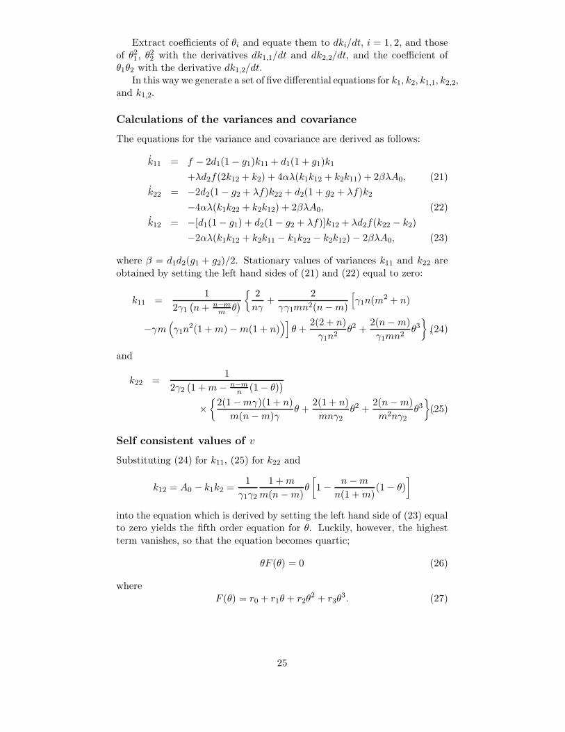
Extract coefficients of θi and equate them to dki/dt, i = 1, 2, and thoseof θ21, θ

22 with the derivatives dk1,1/dt and dk2,2/dt, and the coefficient of

θ1θ2 with the derivative dk1,2/dt.In this way we generate a set of five differential equations for k1, k2, k1,1, k2,2,

and k1,2.

Calculations of the variances and covariance

The equations for the variance and covariance are derived as follows:

k11 = f − 2d1(1 − g1)k11 + d1(1 + g1)k1

+λd2f(2k12 + k2) + 4αλ(k1k12 + k2k11) + 2βλA0, (21)k22 = −2d2(1− g2 + λf)k22 + d2(1 + g2 + λf)k2

−4αλ(k1k22 + k2k12) + 2βλA0, (22)k12 = −[d1(1− g1) + d2(1− g2 + λf)]k12 + λd2f(k22 − k2)

−2αλ(k1k12 + k2k11 − k1k22 − k2k12) − 2βλA0, (23)

where β = d1d2(g1 + g2)/2. Stationary values of variances k11 and k22 areobtained by setting the left hand sides of (21) and (22) equal to zero:

k11 =1

2γ1

(n+ n−m

m θ){

2nγ

+2

γγ1mn2(n−m)

[γ1n(m2 + n)

−γm(γ1n

2(1 +m)−m(1 + n))]θ +

2(2 + n)γ1n2

θ2 +2(n−m)γ1mn2

θ3},(24)

and

k22 =1

2γ2(1 +m− n−m

n (1− θ))

×{

2(1−mγ)(1 + n)m(n−m)γ

θ +2(1 + n)mnγ2

θ2 +2(n−m)m2nγ2

θ3}.(25)

Self consistent values of v

Substituting (24) for k11, (25) for k22 and

k12 = A0 − k1k2 =1

γ1γ2

1 +m

m(n−m)θ

[1 − n −m

n(1 +m)(1 − θ)

]

into the equation which is derived by setting the left hand side of (23) equalto zero yields the fifth order equation for θ. Luckily, however, the highestterm vanishes, so that the equation becomes quartic;

θF (θ) = 0 (26)

whereF (θ) = r0 + r1θ + r2θ

2 + r3θ3. (27)

25

Here

r0 =m(1 + n)γ(n−m)

{γ1γ2

[−m+ 2n(1 + n)

]+ γ

[γ1n

2(1 + n)

+γ2

(− γ1n

2(1 + n) +m[1 + 2n+ (1− γ1)n2])]}

, (28)

r1 = − 1γm

{γ1γ2

[n3 − 4mn(1 + n) +m2(2 + n)

]+ γm

[− γ1n(1 + 5n+ 4n2)

+γ2

(γ1n

2(2 + n) −m[4 + 8n+ (4− γ1)n2])]}

(29)

r2 = −n −m

γm2

{γ1γ2(n−m)2 − γm

[5γ2m(1 + n) + γ1n(3 + 5n)

]}, (30)

r3 =2(n−m)2

m2

{γ2m+ γ1n

}.(31)

26