Mitotic Chromosome Compaction via Active Loop Extrusion_Biology Et Al._2015

BIOLOGICAL SCIENCES: Biophysics and Computational Biology

Mitotic chromosome compaction via active loop extrusion Short title: Chromosome compaction via loop extrusion Anton Goloborodko1, John F. Marko2, Leonid A. Mirny1,3

1 Department of Physics, Massachusetts Institute of Technology, Cambridge MA 02139 2 Department of Molecular Biosciences and Department of Physics and Astronomy, Northwestern University,

Evanston IL 60208 3 Institute for Medical Engineering & Science, Massachusetts Institute of Technology, Cambridge MA 02139 Corresponding author: Leonid Mirny, Institute for Medical Engineering & Science, Massachusetts Institute of

Technology, 77 Mass Ave, Cambridge MA 02139, [email protected], +16174524862 Keywords: prophase, statistical physics, stochastic processes, condensin, structural maintenance of

chromosomes

. CC-BY-NC 4.0 International licensethis preprint is the author/funder. It is made available under a The copyright holder for; http://dx.doi.org/10.1101/021642doi: bioRxiv preprint first posted online June 29, 2015;

mailto:[email protected]

http://dx.doi.org/10.1101/021642

http://creativecommons.org/licenses/by-nc/4.0/

Abstract

During cell division chromosomes are compacted in length by more than a hundred-fold. A wide range of experiments demonstrated that in their compacted state, mammalian chromosomes form arrays of closely stacked consecutive ~100Kb loops. The mechanism underlying the active process of chromosome compaction into a stack of loops is unknown. Here we test the hypothesis that chromosomes are compacted by enzymatic machines that actively extrude chromatin loops. When such loop-extruding factors (LEF) bind to chromosomes, they progressively bridge sites that are further away along the chromosome, thus extruding a loop. We demonstrate that collective action of LEFs leads to formation of a dynamic array of consecutive loops. Simulations and an analytically solved model identify two distinct steady states: a sparse state where loops are highly dynamic but provide little compaction, and a dense state with more stable loops and dramatic chromosome compaction. We find that human chromosomes operate at the border of the dense steady state. Our analysis also shows how the macroscopic characteristics of the loop array are determined by the microscopic properties of LEFs and their abundance. When number of LEFs are used that match experimentally based estimates, the model can quantitatively reproduce the average loop length, the degree of compaction, and the general loop-array morphology of compact human chromosomes. Our study demonstrates that efficient chromosome compaction can be achieved solely by an active loop-extrusion process.

Significance Statement During cell division chromosomes are compacted in length more than a hundred-fold and are folded in arrays of loops. The mechanism underlying this essential biological process is unknown. Here we test whether chromosome compaction can be performed by molecular machines that actively extrude chromatin loops. These machines bind to DNA and progressively bridge sites that are further and further away along the chromosome. We demonstrate that the collective action of loop-extruding machines can fold a chromosome into a dynamic array of loops. Simulated chromosome agrees with compact human chromosomes in its degree of compaction, loop size and the general loop-array morphology. Our study demonstrates that efficient chromosome compaction can be achieved solely by such active loop-extrusion process.


http://dx.doi.org/10.1101/021642


\body

Introduction

During cell division, initially decondensed interphase human chromosomes are compacted in length by more than a hundred-fold into the cylindrical, parallel-chromatid metaphase state. Several lines of evidence suggest that this compaction is achieved via formation of loops along chromosomes (1, 2). First, chromatin loops of

have long been observed via electron microscopy (2–4). These observations served as a basis for the “radial loop” models of the mitotic chromosome (4) and are consistent with optical imaging data (5). Second, theoretical studies showed that compaction into an array of closely stacked loops could explain the observed shape, the mechanical properties and the degree of compaction of mitotic chromosomes (6–8). More recently, the general picture of mitotic chromosomes as a series of closely packed chromatin loops was supported by Hi-C experiments, which measure the frequency of physical contacts within chromosomes (9). The same study independently confirmed the length of the chromatin loops. The mechanism underlying compaction of chromosomes into a stack of loops is unknown. Several lines of evidence suggest that this compaction cannot be achieved by simple mechanisms of chromatin condensation, e.g., “poor solvent” conditions, or non-specific chromatin “cross-linker” proteins. First, the loops are formed overwhelmingly within individual chromatids. Different chromosomes and sister chromatids are not extensively cross-linked to each other as would tend to happen during nonspecific condensation, but instead become individualized during the compaction process. Second, loops are arranged in essentially genomic order and are non-overlapping (9), without the strong overlap of loops that would be expected from nonspecific cross-linking. Finally, metaphase chromosomes compact into elongated structures with a linear arrangement of loops along the main axis. A cross-linking agent would generate surface tension and shrink chromosomes into spherical globules with a random spatial arrangement within a globule (6, 10, 11). In fact, the term “condensation”, which generally refers to the effects of chemical interactions driving phase separation and surface tension, is inappropriate for description of mitotic chromosome compaction where neither effect occurs. Chromatin is clearly being actively compacted during mitosis. An alternative hypothesis is that chromosomes are condensed by enzymatic machines that actively extrude chromatin loops (12, 13). When these enzymes bind to chromosomes, they first link two adjacent sites, but then move both contact points along the chromosome in opposite directions, so that they progressively bridge more distant sites (12). Loop-extruding functions have been observed for other enzymes acting on naked DNA (14–17). Condensin complexes, which play an central role in chromosome compaction (18) and which are present in all domains of life (19), are likely to be a key component of such “loop-extruding factors” (LEFs). A key question is whether LEFs alone are sufficient to drive formation of arrays of non-overlapping loops essential for linear compaction of chromatids, or if other factors are required, e.g., to define the loop bases. In this paper, we model the collective action of loop-extruding factors (LEFs) that dynamically exchange between the nucleoplasm and chromatin fiber. We find that LEFs self-organize into a dynamic array of consecutive loops, which has two distinct steady states: a sparse state where loops are separated by gaps and provide moderate compaction, and a dense state where jammed LEFs drastically compact a long chromatin fiber. These states can be described by a simple analytical model of loop dynamics. We show how the macroscopic characteristics of the loop array are determined by the microscopic properties of the LEFs and their abundance, and we demonstrate that efficient chromosome compaction can be achieved solely by LEFs.

Results

Model for LEFs on a long chromatin segment To understand the dynamics of loops formation and chromatin compaction by loop-extruding factors (LEFs) we carried out stochastic simulations of the process shown in Fig. 1 (13). We focus on the organization and dynamics of loop formation and dissolution without considering 3D organization of the chromatin fiber and assume that emerging topological conflicts can be resolved by topoisomerase II enzymes active during metaphase compaction. We consider a single piece of chromatin fiber of length , occupied by LEFs. We model a LEF very generally as having two “heads” connected by a linker. The LEF heads bind to nearby sites along the chromatin fiber and


http://dx.doi.org/10.1101/021642


proceed to slide away from each other stochastically with an average velocity , thus extruding a loop with rate (Fig. 1a). When the heads of two neighboring LEFs collide, they block each other and halt (Fig 1b). For the LEFs to be able to organize robust loop domains, it is essential that they be able to relocate via

unbinding and rebinding (13). We allow each LEF to dissociate at a rate ⁄ which is independent of their state and location (Fig 1c). When a LEF dissociates, we suppose that it immediately rebinds to a random site elsewhere on the chromosome, where it begins to extrude a new loop (Fig. 1d). The model is fully determined by the four parameters , of which and can be estimated from the experimental studies of

condensins (20–22). We divide the chromosome into sites, so that each site can be occupied by

one LEF head. With each site roughly corresponding to a nucleosome with a DNA linker ( or , a fraction of a size of a condensin complex), our simulated chromosome corresponds to of chromatin fiber.

LEFs can generate a tightly stacked loop array and strong chromosome compaction

In initial simulations we observed that the LEFs generated tightly stacked loops with a high degree of chromatin compaction, despite their constant dissociation (Fig. 1e-g, Supplemental Movie 1). To test that this was a steady state rather than a frozen (glassy) configuration we performed simulations ten times longer than the apparent time needed to reach the steady state, and used a broad range of initial conditions (SI). Simulations converged to states with degree of compaction and distribution of loop size which depended on the control parameters, but were independent of initial states (Fig 1f,g and SI Appendix), providing further support to the existence of a well-defined loop-stacked steady state.

Two characteristic lengths control whether LEFs form dense or sparse chromatin loops

To understand how the microscopic characteristics of the LEFs control the compaction process, we performed simulations systematically exploring the control parameter space. This revealed that there are two distinct steady states of loop-extrusion dynamics in the model (Fig. 2): i) a sparse, poorly compacted state where loops are formed by single LEFs and separated by gaps (Fig. 2c); and ii) a dense state, where the chromosome is compacted into an array of consecutive loops each having multiple LEFs at its base (Fig. 2d). In the sparse state, LEFs do not efficiently condense chromosomes, since even a small fraction of fiber length remaining unextruded in the gaps between loops prevents efficient linear compaction (Figure S7). In the dense state, however, the whole chromosome is folded into a gapless array of loops, where the end of one loop adjacent to the beginning of the following one (Fig 2). Such organization was found to be essential to achieve agreement with Hi-C data for mitotic chromosomes (9). Below we show that realistic LEF abundance (one condensin per ) can give rise to loop sizes of consistent with mitotic Hi-C and earlier direct measurements (3, 21–24) and inferred from Hi-C data (9). These findings suggest a dense state as an attractive model of chromosome compaction.

Two steady states arise from the interplay of two length scales characterizing the LEFs: i) processivity , the average size of a loop extruded by an isolated LEF during its residency time on chromatin; and ii) the

average linear separation between LEFs ⁄ (Fig 2a). When ⁄ , the system resides in the sparse state: LEFs work in isolation, a small fraction of the chromosome is extruded into loops and large gaps between them prevent efficient compaction. In the opposite dense case, when ⁄ , the whole chromosomal fiber is extruded into loops, leading to a high degree of compaction. When the loop coverage is plotted as a function of ⁄ , rather than individual parameters, the curves collapse into a single transition curve

indicative of the central role of ⁄ in controlling the compaction (Figure S1)

Loop organization and dynamics are distinct in the sparse and dense steady states

To understand the process of chromosome compaction by LEFs, we consider the dynamics of loop formation and disassembly. In the sparse state, LEFs rarely interact; each loop is extruded by a single LEF and it disappears once the LEF dissociates, leading to a highly dynamic state with a rapid ( ) turnover of loops (Fig S1a, SI Appendix). Since LEFs extrude loops continuously and the distribution of LEFtheir residence times is exponential, the distribution of loop size is exponential too (Figure S2). Two aspects of the loop organization control the dense state dynamics: i) loops have no gaps between each other; and (ii) individual loops are reinforced by multiple LEFs, i.e. several LEFs are stacked on top of each


http://dx.doi.org/10.1101/021642


other at the base of a loop (13). Both phenomena result from the competition for chromosomal fiber among abundant LEFs. The gaps disappear because, in the dense state, LEFs have enough time to extrude all available fiber until colliding with adjacent LEFs. Abundant collisions lead to a non-exponential distribution of loop sizes (Figure S2, SI Appendix). Loop reinforcement is also caused by LEF collisions (Fig 3): every time a new LEF binds within an existing loop, it re-extrudes this loop until colliding with the LEF residing at the loop base. As a result, each loop is stabilized by multiple LEFs at its base. The absence of gaps and the reinforcement of loops preserve the structure of loops on the timescales (Fig S1b, SI Appendix): loops cannot grow because their LEFs are blocked by the neighbors, and they do not disband when individual LEFs dissociate, as remaining LEFs support them. Thus, the loops of a condensed chromosome are maintained despite continuously exchanging LEFs, like the planks in the ship of Theseus (25).

Steady state loop dynamics is controlled by competition between loop death and division

To develop an analytical model of the system’s steady state we consider its dynamics. Loops in the dense state are not completely static: Two stochastic processes, loop “death” and loop “division”, change the structure of the loop array and drive self-organization of the steady state. A loop “dies” when the number of LEFs at its base supporting it fluctuates to zero. When all LEFs dissociate, neighboring LEFs become unblocked and extrude the released fiber into their own loops (Fig 4a). We compute the rate at which a stack of LEFs supporting a loop of size can stochastically fluctuate to zero. The stack can shrink due to LEFs dissociation (at rate ) and can grow due to association of new LEFs to the loop (at

rate

). Fluctuations of the LEF stack size are equivalent to the stochastic immigration-death

process, for which the rate of fluctuation to zero can be computed as

(SI Appendix) (26).

A loop “divides” into two smaller loops when two LEFs land within a single loop almost simultaneously and extrude two smaller consecutive loops (Fig 4b). These newly created loops become subsequently reinforced by other LEFs that land into them. The original “parent” loop, on the contrary, is effectively cut off from the supply of reinforcing LEFs, and disintegrates on a timescale , with the two child loops taking its place. The rate-limiting process for loop division is the landing of two LEFs onto the same loop, giving an estimate for the

rate of division:

(

)

(SI Appendix). These scaling laws accurately predict the dynamics of loop

birth and death (Fig. 4c, d) In the steady state, the number of loops is approximately constant. By equating the rate of loop creation by division to the rate of loop death, the average loop size is obtained as:

(√

) (

) (1)

and the average number of LEFs per loop is:

(√

) (

) (2)

where is the Lambert W function. Our analytical model agrees with simulations (Fig 4e) and explains how the number of LEFs and their microscopic properties affect the morphology of compacted chromosomes. First, Eq. (1) and (2) show that is the key control parameter of the system, which determines not only the state of the system (sparse vs dense), but also loop sizes and the degree of loop reinforcement in the dense state. Using these scaling laws plus available experimental data we can estimate LEF processivity and dynamic state for human metaphase chromosomes. The average loop length has been estimated by miroscopy and via

modeling of Hi-C data as (3, 9, 23, 24). The spacing between bound condensin molecules was measured as (21). Using these values we obtain a range of ⁄ that is shown on Fig 4e

and corresponds to ⁄ . These values shows that human mitotic chromosomes operate at the lower bound of the dense state, have each loop reinforced by LEFs, and human LEF have processivity .


http://dx.doi.org/10.1101/021642


Second, our analysis allows to compute the degree of chromosomal compaction by LEFs. Since the length of a compacted chromosome in the gapless dense state equals the sum of the widths of the loop bases, (Fig 1E),

the coefficient of chromosomal compaction is ⁄ . While addition of extra LEFs leads to better loop reinforcement, it also makes loops shorter ( ⁄ ) and thus reduces the degree of chromosomal

compaction (Fig S7, SI Appendix). For the loop base size close to the chromatin fiber diameter

we obtain the degree of compaction ⁄ . Interestingly, our estimate for the compaction achieved through folding of a chromosome into a gapless array of loops is in a good agreement with the

experimentally measured degree of human chromosome compaction in mid-prophase ( ) (27). Third, our model predicts how the loop array morphology changes in response to biological perturbations. Specifically, factors that decrease the speed of loop extrusion or reduce LEF residence time will decrease the processivity and thus decrease the average loop size, degree of loop reinforcement and the degree of chromatid compaction. The effects of LEF overexpression depend on the state of the system: for sparse loop arrays, it does not affect the average loop size and only increases the number of loops and, thus the degree of compaction. In the dense systems, LEF overexpression decreases the average loop size and degree of compaction, but increases the degree of loop reinforcement. Finally, this analytical model shows how LEFs robustly self-organize chromosomes into a globally stable steady state. The rates of death and division and scale differently with the loop length: large

loops are more likely to divide into smaller ones ( ), and smaller loops are more likely to die

( ) allowing neighboring loops to grow. This negative feedback drives the system to a steady state with a relatively narrow distribution of loop lengths. These results indicate that loop sizes and hence chromosome diameter and length will be sensitive to concentrations of LEFs while the overall morphology as a gapless array of consecutive loops will remain unchanged as long as the system remains in the dense state.

Discussion Our model of loop-extrusion provides a resolution of the puzzle of how roughly nanometer-sized enzyme complexes can drive the regular organization of a chromosome at scales well beyond a micron, as occurs in eukaryote cells during mitosis. A fundamental problem with almost any mechanism based on non-specific crosslinking of chromatin fibers is that chromosomes will end up crosslinked together: our model avoids this fate by having LEFs bind to chromatin at one location and then actively extrude loops without the possibility of forming inter-chromosome attachments. Through unbinding, rebinding, and re-extrusion, enzymatic machines of this type gradually build larger loops anchored by multiple LEFs, eventually reaching a steady state. A key feature of our model is that the compaction process proceeds by a combination of stochastic loop “death” and “division” events, which gradually but not strictly monotonically leads to a highly compacted chromosome. Compaction driven by LEFs is distinct from the usual polymer “condensation” occurring under “poor solvent” conditions. Unlike proposed linear compaction, nonspecific adhesion of chromatin fibers to one another would generate surface tension, driving adhesion of chromosomes together into spherical masses of chromatin (11), increasing entanglement and working against chromosome segregation and individualization (8, 13). An important feature of the LEF-compacted state is that despite its robust structure, it is entirely dependent on DNA connectivity; intermittent cleavage of DNA alone can lead to dissolution of the entire chromosome, as has been observed experimentally (28, 29). We emphasize that in the compacted steady state the loops have a well-defined size, and that inside the chromosome the LEFs establish internal tension, rather than the surface tension generated by nonspecific crosslinking. This internal tension is an essential contributor to the uniform folding and well-regulated cylindrical morphology of chromatids, and also generates repulsive forces between folded chromosomes essential to segregation of sister chromatids and individualization of different chromosomes (6). Note that achieving a compacted steady state by this mechanism can be a slow process, i.e. it would require

, while the turnover rate for condensin was measured to be at least a few minutes (20). However, we found that gradual or step-wise loading/activation of LEFs can lead to a significant speed-up of


http://dx.doi.org/10.1101/021642


the process (SI Appendix). For the optimal activation rate, the compact steady state can be achieved in a fraction of time (see Fig S9, SI Appendix). A sign of this dynamics occurring in vivo would be its gradual up-regulation/activation of condesin during early chromosome compaction. On the other hand, if there are too few LEFs we have found that a distinct, disordered, poorly compacted chromosome steady state occurs. This outcome has been observed in experiments where condensins were interfered with, both in cells (30) and in Xenopus egg extracts (18, 30). Modulation of chromosome structure also has been observed to occur through development, for example in Xenopus, where mitotic chromosomes become gradually shorter and fatter with maturation (31); this gradual change in chromosome morphology could be due to changes in LEF amount or activity with development. While the mechanisms of loop extrusion remain unknown, a relative simple molecular organization of a protein complex could produce loop-extruding activity. A LEF composed of two connected heads, each able to move along chromatin fiber processively, can achieve a loop extrusion activity. Moreover relative dynamics of the two heads (motors) does not have to be coordinated. In fact, of four possible relative orientation of heads’ directions ( , , , ), two ( , ) produce LEFs that slide along chromatin without loop extrusion,

one ( ) makes LEFs with heads pushing against each other and thus stuck on chromatin, and the last one ( ) makes LEFs with heads moving away from each other and thus extruding loops. It remains to be seen how these functions are implemented in structures of SMC complexes (cohesins and condensins) that have enzymatic (ATP-hydrolyzing) domains. We note that our model does not discern between condensin I and condensin II, and also that the considered compaction process is the prophase compaction driven by condensin II (30). Experiments aimed at disrupting LEFs would perhaps be best targeted at condensin II; however other proteins may be involved as condensin II by itself is not thought to have motor function. Intriguingly, the motor KIF4A has been shown to be involved with mitotic chromosome compaction (32); it is conceivable that condensins are somehow aided in a LEF function by a separate motor molecule such as KIF4A. Alternately, condensins may be able to cooperatively organize so as to generate contractile LEF behavior, for example by “directional polymerization” (13).

Materials and methods Simulations were performed using the Gillespie algorithm (13, 33). The Python code performing the simulations of loop extrusion and the data analysis and is available online at https://bitbucket.org/golobor/loop-extrusion-1d. See SI Appendix for details of simulations.

Acknowledgements Work at NU was supported by the NSF through Grants DMR-1206868 and MCB-1022117, and by the NIH through Grants GM105847 and CA193419. Work at MIT was supported by the NIH through Grants GM114190 R01HG003143. We are grateful to Maxim Imakaev, Geoffrey Fudenberg, Christopher McFarland, Nezar Abdennur, Rotem Gura, Mehran Kardar and the members of MIT Biophysics for productive discussions.


https://bitbucket.org/golobor/loop-extrusion-1d

https://bitbucket.org/golobor/loop-extrusion-1d

http://dx.doi.org/10.1101/021642


References

1. Maeshima K, Laemmli UK (2003) A two-step scaffolding model for mitotic chromosome assembly. Dev Cell 4(4):467–80.

2. Maeshima K, Eltsov M, Laemmli UK (2005) Chromosome structure: improved immunolabeling for electron microscopy. Chromosoma 114(5):365–75.

3. Paulson JR, Laemmli UK (1977) The structure of histone-depleted metaphase chromosomes. Cell 12(3):817–828.

4. Marsden M, Laemmli U (1979) Metaphase chromosome structure: evidence for a radial loop model. Cell 17(August):849–858.

5. Liang Z, et al. (2015) Chromosomes Progress to Metaphase in Multiple Discrete Steps via Global Compaction/Expansion Cycles. Cell 161(5):1124–1137.

6. Marko JF, Siggia ED (1997) Polymer models of meiotic and mitotic chromosomes. Mol Biol Cell 8(11):2217–31.

7. Zhang Y, Heermann DW (2011) Loops Determine the Mechanical Properties of Mitotic Chromosomes. PLoS One 6(12):e29225.

8. Marko JF (2008) Micromechanical studies of mitotic chromosomes. Chromosome Res 16(3):469–97.

9. Naumova N, et al. (2013) Organization of the mitotic chromosome. Science 342(6161):948–53.

10. Grosberg A, Khokhlov A (1994) Statistical Mechanics of Macromolecules (AIP, Woodbury, NY).

11. Strick R, Laemmli UK (1995) SARs are cis DNA elements of chromosome dynamics: Synthesis of a SAR repressor protein. Cell 83(7):1137–1148.

12. Nasmyth K (2001) Disseminating the genome: joining, resolving, and separating sister chromatids during mitosis and meiosis. Annu Rev Genet 35:673–745.

13. Alipour E, Marko JF (2012) Self-organization of domain structures by DNA-loop-extruding enzymes. Nucleic Acids Res 40(22):11202–12.

14. Allen DJ (1997) MutS mediates heteroduplex loop formation by a translocation mechanism. EMBO J 16(14):4467–4476.

15. Prasad TK, et al. (2007) A DNA-translocating Snf2 molecular motor: Saccharomyces cerevisiae Rdh54 displays processive translocation and extrudes DNA loops. J Mol Biol 369(4):940–53.

16. Crampton N, et al. (2007) Fast-scan atomic force microscopy reveals that the type III restriction enzyme EcoP15I is capable of DNA translocation and looping. Proc Natl Acad Sci 104(31):12755–12760.

17. Seidel R, et al. (2004) Real-time observation of DNA translocation by the type I restriction modification enzyme EcoR124I. Nat Struct & Mol Biol 11(9):838–843.

18. Hirano T, Mitchison TJ (1994) A heterodimeric coiled-coil protein required for mitotic chromosome condensation in vitro. Cell 79(3):449–58.


http://dx.doi.org/10.1101/021642


19. Hirano T (2012) Condensins: universal organizers of chromosomes with diverse functions. Genes Dev 26(15):1659–78.

20. Gerlich D, Hirota T, Koch B, Peters J-M, Ellenberg J (2006) Condensin I stabilizes chromosomes mechanically through a dynamic interaction in live cells. Curr Biol 16(4):333–44.

21. Fukui K, Uchiyama S (2007) Chromosome protein framework from proteome analysis of isolated human metaphase chromosomes. Chem Rec 7(4):230–7.

22. Takemoto A, Kimura K, Yokoyama S, Hanaoka F (2004) Cell cycle-dependent phosphorylation, nuclear localization, and activation of human condensin. J Biol Chem 279(6):4551–9.

23. Jackson D, Dickinson P, Cook PR (1990) The size of chromatin loops in HeLa cells. EMBO J 9(2):567–71.

24. Earnshaw WC, Laemmli UK (1983) Architecture of metaphase chromosomes and chromosome scaffolds. J Cell Biol 96(1):84–93.

25. Plutarch (75AD) Life of Theseus.

26. Pinsky MA, Karlin S (2011) An Introduction to Stochastic Modeling (Academic Press).

27. Yunis JJ (1981) Mid-prophase human chromosomes. The attainment of 2000 bands. Hum Genet 56(3):293–298.

28. Poirier MG, Marko JF (2003) Micromechanical Studies of Mitotic Chromosomes. Chromosome Research, pp 75–141.

29. Sun M, Nishino T, Marko JF (2013) The SMC1-SMC3 cohesin heterodimer structures DNA through supercoiling-dependent loop formation. Nucleic Acids Res 41(12):6149–6160.

30. Ono T, et al. (2003) Differential contributions of condensin I and condensin II to mitotic chromosome architecture in vertebrate cells. Cell 115(1):109–21.

31. Micheli G, Luzzatto A, Carrì M, de Capoa A, Pelliccia F (1993) Chromosome length and DNA loop size during early embryonic development of Xenopus laevis. Chromosoma 102(7):478–83.

32. Mazumdar M (2004) Human chromokinesin KIF4A functions in chromosome condensation and segregation. J Cell Biol 166(5):613–620.

33. Gillespie DT (1977) Exact stochastic simulation of coupled chemical reactions. J Phys Chem 81(25):2340–2361.


http://dx.doi.org/10.1101/021642


Figure Legends Figure 1. Simulations of chromosome compaction by loop extruding factors (LEFs). The action of LEFs can be simulated using a one-dimensional lattice model with four dynamic rules (a)-(d): (a) LEFs extrude loops by moving the two connected heads along the chromosome, (b) LEF heads block each other, (c) LEFs dissociate from chromatin, and (d) LEFs in the solution rebind to the chromosome. (e) Simulations show that LEFs can fold a chromosome into an array of consecutive loops. The diagram shows the loops formed by LEFs in a simulation with , , , after 45000 time steps. (f),(g) The system of LEFs on a long chromatin fiber converges to a steady state. The steady distribution of loop sizes and the degree of compaction depends on the control parameters, but is independent of initial state. Results are shown for different simulation parameters and starting conditions; data for each curve is averaged over 10 simulation replicas.

Figure 2. Simulations of LEFs reveal two distinct steady states. (a-b) The properties of loop arrays formed by LEFs, such as the portion of the chromosome extruded into loops, the portion of branched loops and the number of LEFs per loop, depend on the dimensionless ratio ⁄ . This ratio defines the two steady states of

the system: (c) the sparse state ( ⁄ ) where the loops are supported by single LEFs and separated by big loop-free gaps and (d) the dense state ( ⁄ ) where the whole chromosome is extruded into an array of consecutive loops supported by multiple LEFs. In both steady states, the loops are not branched (a). The

vertical dotted lines at ⁄ and roughly show the transition region. Figure 3. The mechanism of loop reinforcement in the dense state. Upon binding to an existing loop, a LEF re-extrudes it and stacks on top of the LEFs already supporting the loop.

Figure 4. The model of loop death and division explains the origin of the dense steady state. (a) Loops occasionally disassemble when the number of reinforcing LEFs fluctuates to zero. The chromatin of the disassembled loop is immediately extruded into the adjacent loops. (b) A loop splits upon simultaneous landing of two reinforcing LEFs. The rates of loop death (c) and division (d) in the dense state can be estimated using simple analytical formulas (red dots) or more accurate computational models (blue dots). (f) In the dense state, the steady-state balance between loop death and division provides an approximate analytical expression for the average loop length (the red line). In the sparse state, the average loop length is predicted to be equal (the red line). Both predictions agree well with the simulations (the black line). The four horizontal overlapping

gray bands show the available independent experimental estimates of in mitotic human

chromosomes: (3), (24), (23) and (9) and (21).

Abbreviations

LEF – loop extuding factor

SMC – structural maintenance of chromosomes


http://dx.doi.org/10.1101/021642


Figures

Figure 1. Simulations of chromosome compaction by loop extruding factors (LEFs). The action of LEFs can be simulated using a one-dimensional lattice model with four dynamic rules (a)-(d): (a) LEFs extrude loops by moving the two connected heads along the chromosome, (b) LEF heads block each other, (c) LEFs dissociate from chromatin, and (d) LEFs in the solution rebind to the chromosome. (e) Simulations show that LEFs can fold a chromosome into an array of consecutive loops. The diagram shows the loops formed by LEFs in a simulation with , , , after 45000 time steps. (f),(g) The system of LEFs on a long chromatin fiber converges to a steady state. The steady distribution of loop sizes and the degree of compaction depends on the control parameters, but is independent of initial state. Results are shown for different simulation parameters and starting conditions; data for each curve is averaged over 10 simulation replicas.


http://dx.doi.org/10.1101/021642


Figure 2. Simulations of LEFs reveal two distinct steady states. (a-b) The properties of loop arrays formed by LEFs, such as the portion of the chromosome extruded into loops, the portion of branched loops and the number of LEFs per loop, depend on the dimensionless ratio ⁄ . This ratio defines the two steady states of

the system: (c) the sparse state ( ⁄ ) where the loops are supported by single LEFs and separated by big loop-free gaps and (d) the dense state ( ⁄ ) where the whole chromosome is extruded into an array of consecutive loops supported by multiple LEFs. In both steady states, the loops are not branched (a). The

vertical dotted lines at ⁄ and roughly show the transition region.


http://dx.doi.org/10.1101/021642


Figure 3. The mechanism of loop reinforcement in the dense state. Upon binding to an existing loop, a LEF re-extrudes it and stacks on top of the LEFs already supporting the loop.


http://dx.doi.org/10.1101/021642


Figure 4. The model of loop death and division explains the origin of the dense steady state. (a) Loops occasionally disassemble when the number of reinforcing LEFs fluctuates to zero. The chromatin of the disassembled loop is immediately extruded into the adjacent loops. (b) A loop splits upon simultaneous landing of two reinforcing LEFs. The rates of loop death (c) and division (d) in the dense state can be estimated using simple analytical formulas (red dots) or more accurate computational models (blue dots). (f) In the dense state, the steady-state balance between loop death and division provides an approximate analytical expression for

the average loop length (the red line). In the sparse state, the average loop length is predicted to be equal (the red line). Both predictions agree well with the simulations (the black line). The four horizontal overlapping

gray bands show the available independent experimental estimates of in mitotic human

chromosomes: (3), (24), (23) and (9) and (21).


http://dx.doi.org/10.1101/021642


Supplementary Information Appendix

Mitotic chromosome compactionvia active loop extrusionContents1 Materials and methods. 3

2 The two regimes of LEFs on a chromosome. 32.1 Loops have different dynamics in the sparse and dense regimes. . 42.2 The distribution of loop lengths is exponential in the sparse

regime and normal in the dense regime. . . . . . . . . . . . . . . 52.3 Gaps disappear exponentially with λ/d. . . . . . . . . . . . . . . . 6

3 The theory of self-organization of loop arrays in the denseregime. 73.1 In the dense regime, loops have stable lengths and fluctuating

numbers of reinforcing LEFs. . . . . . . . . . . . . . . . . . . . . 73.2 The number of LEFs in a loop is approximately Poisson-distributed

around ℓ/d. . . . . . . . . . . . . . . . . . . . . . . . . . . . . . . . 73.3 The lifespan of reinforced loops increases exponentially with their

length. . . . . . . . . . . . . . . . . . . . . . . . . . . . . . . . . . 93.4 Loops in the dense regime stochastically divide in two. . . . . . . 103.5 The balance between loop death and division gives rise to the

steady state of the dense regime. . . . . . . . . . . . . . . . . . . 103.6 Maximal lengthwise compaction is achieved on the lower border

of the dense regime. . . . . . . . . . . . . . . . . . . . . . . . . . 123.7 The maximal degree of total compaction depends on the length

of the chromosome and the size of LEFs. . . . . . . . . . . . . . . 133.8 Gradual activation of LEFs speeds up convergence to the steady

state. . . . . . . . . . . . . . . . . . . . . . . . . . . . . . . . . . . 14

4 Corrections to the theory of self-organization of loop arrays. 184.1 The theory of stochastic processes provides an exact expression

for the lifespan of loops. . . . . . . . . . . . . . . . . . . . . . . . 18

1


http://dx.doi.org/10.1101/021642


4.2 Loops supported by a single LEF can die immediately. . . . . . . 204.3 Accounting for immediate death gives a simple and accurate es-

timate for the rate of loop death. . . . . . . . . . . . . . . . . . . 214.4 The lifespan of a loop after interruption of reinforcement is ap-

proximately Gumbel-distributed. . . . . . . . . . . . . . . . . . . 224.5 Selection for the minimal daughter loop size slows down loop

division. . . . . . . . . . . . . . . . . . . . . . . . . . . . . . . . . 234.6 Immediate death of daughter loops slows down loop division. . . 244.7 Loop size selection and immediate death affects daughter loops

independently. . . . . . . . . . . . . . . . . . . . . . . . . . . . . 25

5 Glossary and mathematical notation 26

References 29

2


http://dx.doi.org/10.1101/021642


1 Materials and methods.We study the action of loop extruding factors (LEFs) using the previously de-scribed model [1]. In this model, we model a chromosome as a one-dimensionallattice with L sites with N LEFs. Each LEF is represented as a pair of “heads”,each occupying an individual site on the chromosome. The positions of LEFheads are stochastically updated using the Gillespie algorithm with four rules:

1. The two heads of each LEF stochastically step away from each other withthe average rate v.

2. The heads of different LEFs cannot step over each other and thus stopextrusion upon reaching another LEF. However, the two heads of the sameLEF extrude loops independently and if one head of a LEF is blocked,another head continues extrusion.

3. LEFs stochastically unbind from the fiber with the rate of 1τ , where τ is

the average residence time.

4. Free LEFs immediately rebind to the chromatin fiber at a random uni-formly chosen pair of adjacent sites.

In this study we modeled 12Mb of chromatin fiber, close to the size of thesmallest human chromosomal arm 21p (12.7 Mb). Without loss of generality,we divided the fiber into a lattice of L = 60000 cells of 200 bp each, roughlythe size of a nucleosome with a DNA linker. We simulated systems with N =100, 400, 800, 1200 and 1600 LEFs, where 400-1200 LEFs corresponded to theexperimental estimates of the abundance of condensin in mitotic human cells (1per 10-30kb) [2, 3]. The speed of extrusion v varied in a broad range between1 and 100 sites per time unit and the residence time τ varied between 10 and105 time units. At the beginning of each simulation, LEFs were distributedrandomly along the chromosome with both heads in adjacent lattice sites. Wesimulated each system for 104 · τ units of time, with 10 simulations per eachparameter set.

We found that the average loop length ℓ in the steady state did not dependon the initial positions of LEFs, with only 1 out of 75 tested parameter setsfailing the Bonferroni-corrected one-way ANOVA comparison of ℓ between tenrandomly initiated replicas. Additionally, we found that the same final values ofℓ were achieved if the system was initiated with 20 or 60 loops of equal length,each supported by closely stacked LEFs.

2 The two regimes of LEFs on a chromosome.We found that the system of LEFs has two distinct regimes: the sparse regime,where loops are formed by individual LEFs and are separated by gaps, andthe dense regime, where loops are supported by multiple LEFs and cover thechromosome completely. The transition between the two regimes occurs when

3


http://dx.doi.org/10.1101/021642


we increase the parameter λd , where λ = 2vτ is the LEF processivity, i.e. the

average length of a loop extruded by an obstructed LEF over its residence timeon chromatin and d = L

N is the average linear separation between LEFs. Oursimulations suggested that this ratio, and not each of the parameters alone,determines the average loop coverage, i.e. the portion of chromatin extrudedinto loops (Figure S1).

a b c

Figure S1: Loop coverage as (a) a function of the LEF processivity λ for differentnumbers of LEFs N and (b) as a function of N for several values of λ. (c) Thecurves collapse when plotted relative to the ratio λ/d = λN/L.

2.1 Loops have different dynamics in the sparse and denseregimes.

We found that loops in the two regimes of LEFs display very different dynamics(Fig. S2). As a proxy for the timescale of loop stability we measured the au-tocorrelation time of the LEF footprint on chromatin. This measure allowed usto estimate the characteristic times of change in loop structures across multipleorders of magnitude. In the sparse regime, autocorrelation time is much shorterthan τ , inversely proportional to the speed of loop extrusion v and independentof other parameters, indicating unobstructed loop extrusion by LEFs. In thedense regime, dynamics slows down drastically and the autocorrelation time ex-ceeds τ , showing that the loop structure persists after multiple rounds of LEFexchange. In the dense regime, the autocorrelation time normalized by τ scalesas√

λd .

4


http://dx.doi.org/10.1101/021642


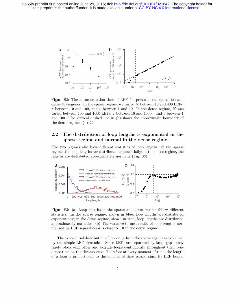
a b

Figure S2: The autocorrelation time of LEF footprints in the sparse (a) anddense (b) regimes. In the sparse regime, we varied N between 10 and 400 LEFs,τ between 10 and 100, and v between 1 and 10. In the dense regime, N wasvaried between 100 and 1600 LEFs, τ between 10 and 10000, and v between 1and 100. The vertical dashed line in (b) shows the approximate boundary ofthe dense regime, λ

d ≈ 20.

2.2 The distribution of loop lengths is exponential in thesparse regime and normal in the dense regime.

The two regimes also have different statistics of loop lengths: in the sparseregime, the loop lengths are distributed exponentially; in the dense regime, thelengths are distributed approximately normally (Fig. S3).

a b

Figure S3: (a) Loop lengths in the sparse and dense regime follow differentstatistics. In the sparse regime, shown in blue, loop lengths are distributedexponentially; in the dense regime, shown in read, loop lengths are distributedapproximately normally. (b) The variance-to-mean ratio of loop lengths nor-malized by LEF separation d is close to 1.0 in the dense regime.

The exponential distribution of loop lengths in the sparse regime is explainedby the simple LEF dynamics. Since LEFs are separated by large gaps, theyrarely block each other and extrude loops continuously throughout their resi-dence time on the chromosome. Therefore at every moment of time, the lengthof a loop is proportional to the amount of time passed since its LEF bound

5


http://dx.doi.org/10.1101/021642


to the chromosome. In the theory of renewal processes this amount of time iscalled age and, like the residence time of LEF, it is distributed exponentiallyaround its mean of τ [4]. Thus, the lengths of loops in the sparse regime alsobecome exponentially distributed with the average length of ℓ = λ = 2vτ .

In the dense regime, the distribution of loop lengths can be approximatedby the normal distribution, with the mean and the standard deviation thatdepend on the parameters of the system. Interestingly, the variance-to-meanratio of loop lengths in units of LEF separation d is very close to unity in thedense regime. Our theory presented below explains why the distribution ofloop lengths ℓ has a non-zero peak and predicts its approximate location, butit cannot predict the exact analytical form of this distribution nor its width.

2.3 Gaps disappear exponentially with λ/d.The simple structure of loops in the sparse regime allows us to explain theobserved dependence of loop coverage 1 − g on λ

d (where g is the portion ofgaps, i.e. the portion of chromatin fiber that is not extruded into any loop)(Fig. S4). When we increase the number of LEFs N , while keeping L, v and τfixed, the portion g of gaps should decrease. This dependence is, however, notlinear: as more chromatin fiber is extruded into loops, it becomes increasinglylikely for LEFs to form nested loops (i.e. bind within already extruded loops)and thus not contribute to the overall loop coverage. Therefore, every new LEFin the system that lands in a gap between loops increases loop coverage byℓL ≈ λ

L (i.e. reduces the portion of gaps g by the same amount). The chance ofa LEF landing in a gap is g, which gives us a simple differential equation:

dg

dN= −λ

Lg,

g = e−λd (S1)

Comparison with the simulations (Figure S4) shows that this solution cap-tures the transition between the sparse and the dense regimes, but noticeablyunderestimates the portion of gaps as we approach the dense regime, 1 < λ

d < 20.This discrepancy is due to the growing difference between ℓ and λ in the denseregime (see below).

6


http://dx.doi.org/10.1101/021642


Figure S4: The comparison of the theoretically predicted loop coverage withthe results of the simulations. The vertical dashed lines show the approximateboundaries of the sparse and dense regimes.

3 The theory of self-organization of loop arraysin the dense regime.

3.1 In the dense regime, loops have stable lengths andfluctuating numbers of reinforcing LEFs.

At λ ≫ d, gaps between loops disappear and the system transitions into thedense regime. The condition λ ≫ d means that LEFs can potentially formloops that are much larger than the amount of chromatin available to each ofthem, so the size of the extruded loop become limited by collisions betweenLEFs. Also, because there are no gaps between loops, LEFs that rebind to thechromatin always start new loops within other already existing loops. Finally, aswe show in the main text, in the extreme dense regime loop branching becomesincreasingly rare and the majority of LEFs just stack on top of each other,forming reinforced loops. Thus, LEFs in the dense regime fold chromatin intoan array of consecutive reinforced loops. The length ℓ of each reinforced loop isrelatively stable: supported by multiple LEFs, it does not disappear or shrink,when some of them unbind, but it cannot grow either, because its LEFs areblocked by the neighbors. Conversely, the number of LEFs n in each reinforcedloop constantly fluctuates: the loops constantly lose LEFs due to their unbindingand receive new LEFs that rebind to the chromosome from the solution. Belowwe describe the fluctuations of loop structure in the dense regime and show howthey lead to a globally stable steady state.

3.2 The number of LEFs in a loop is approximately Poisson-distributed around ℓ/d.

Let us derive the distribution of the number of LEFs n supporting a singlereinforced loop of length ℓ. The loop loses LEFs due to their dissociation from

7


http://dx.doi.org/10.1101/021642


the chromatin fiber. Since individual LEFs unbind with a rate µ = 1τ , the overall

rate of LEF loss depends on n and equals

µn = nµ =n

τ(S2)

The loop also receives a flux of incoming LEFs that bind back to the chro-mosome from the solution. In our simple model, LEFs rebind to random sitesand thus have a chance ℓ

L of landing within the chosen loop. As a result, thebody of the loop serves as an antenna: the larger the loop is, the more LEFsit receives. At every moment of time, LEFs unbind and immediately rebind tothe chromosome with the rate N · 1

τ , so that the rate r of LEF binding to thechosen loop equals

r =N

τ· ℓ

L=

1

τ

ℓ

d(S3)

This stochastic gain and loss of LEFs produces fluctuations of the numberof LEFs in the loop. The equations S2 and S3 allow us to find the probabilitypn for the loop to have n LEFs. In a population of loops of equal length ℓ, thefraction pn of loops supported by n LEFs changes over time because of threefactors: a) these loops gain or lose LEFs with a combined rate r+µn , b) loopswith n− 1 LEFs gain LEFs at rate r and c) loops with n+ 1 LEF lose LEFs atrate µn+1. The dynamics of the fraction pn is then described with:{

dpn

dt = − (r + µn) pn + rpn−1 + µn+1pn+1, n > 1dp1

dt = − (r + µ1) p1 + µ2p2, n = 1

The loss of the last LEF is irreversible and loops without LEFs disappear.In order to find a quasi steady state distribution of pn described by dpn

dt = 0,we have to ignore this fact for now and set µ1 = 0. This gives us the followingsystem of equations [5]:{

(r + µn)pn = rpn−1 + µn+1pn+1, n > 1

rp1 = µ2p2

The solution of this system shows that the number of LEFs n, n ≥ 1 in aloop is Poisson-distributed:

pn =n−1∏i=1

riµi+1

p1 =1

n!

(r

µ

)n1

erµ − 1

We can relate this distribution to the size of the loop and density of LEFsusing the expressions (S3) and (S2):

pn (ℓ/d) =1

n!(ℓ/d)

n 1

eℓ/d − 1(S4)

8


http://dx.doi.org/10.1101/021642


The average number of LEFs n in a loop then equals:

n =ℓ

d

1

1− e−ℓ/d(S5)

This expression highlights the importance of the length scale d: the lengthof a loop expressed in units of LEF separation d is approximately equal to theaverage number of LEFs in this loop. Below we will often use the loop lengthnormalized by d:

ℓd ≡ ℓ

d(S6)

such that:

n ≈ ℓd (S7)

3.3 The lifespan of reinforced loops increases exponen-tially with their length.

The derived distribution (S4) of the number of LEFs per loop allows us toestimate the average lifespan of a loop t. Loops get disassembled when theylose their last LEF. Therefore, the rate of loop death can be estimated as:

Rdeath ≈ µp1 =1

τ

ℓdeℓd − 1

≈ 1

τℓde

−ℓd (S8)

And the average lifespan t of a loop of length ℓd is

t =1

Rdeath≈ τ

eℓd − 1

ℓd(S9)

The asymptotic dependence of t on the length of the normalized loop lengthℓd is then:

tasymp =1

Rasympdeath

≈ τeℓd

ℓd(S10)

The equation (S10) reveals that the lifespan of a loop grows almost expo-nentially with its length. Thus, reinforcement makes longer loops essentiallyimmortal: for example, loops with length ℓd = 6.5 live 100 times longer thanindividual LEFs, and those with ℓd = 9 live 1000 times longer. However, theeffects of reinforcement are significant only for longer loops (ℓd ≳ 3.5) with thelifespan extension to 10τ and more.

The simple functional form of Eq. (S10) allows us to use it in analyticalcalculations. However, in its derivation we assumed that loop death does notperturb the distribution of n, which is not necessarily true. In chapter (4.1),we will derive the expression for t without this assumption and show that ourestimates (S9) and (S10) are, in fact, very accurate.

9


http://dx.doi.org/10.1101/021642


3.4 Loops in the dense regime stochastically divide in two.Loops in the dense regime divide when two LEFs land within the same loopand extrude two separate loops instead of stacking on top of one another. Bothdaughter loops then start receiving reinforcing LEFs, thus, cutting the suppliesoff the mother loop. This causes the mother loop to disassemble on the timescaleof several τ (for more accurate estimate, see Chapter (4.4)) and the two daughterloops take its place. This process creates new loops on the chromatin in thedense regime.

We can estimate how the rate of loop division depends on the parametersof the system. LEFs land into a loop of size ℓ with a rate of Nℓ

τL = 1τ

ℓd . A loop

divides when the second LEF lands before the first LEF has fully expanded tothe loop borders, within a time window of ∼ ℓ

2v . Thus, the rate of loop divisionscales as:

Rdiv ∼(1

τ

ℓ

d

)2ℓ

2v=

1

τℓ3d

d

λ(S11)

However, these two LEFs can still stack on one another. In fact, as the firstLEF extrudes a bigger and bigger loop, there is less chance for the second LEFto land outside of its loop. Thus, a more accurate general expression for Rdiv

should look like:

Rdiv = r2ˆ ∞

0

Pdiv(ℓ, t) dt, (S12)

where Pdiv(ℓ, t) is the probability for two LEFs to divide a loop of length ℓif they land with a time delay t.

The loop splits if the second LEF lands outside of the loop extruded by thefirst. Integrating over all possible positions of the two LEFs, x1 and x2, we get:

Pdiv(ℓ, t) =1

l2

ˆ l

0

dx1

ˆ l

0

dx2 (1x2>x1+vt + 1x2<x1−vt) = (S13)

=

(1− vt

ℓ

)2

Here, 1condition is the indicator function, which equals 1 is the condition istrue and 0 otherwise. The expression for Rdiv is then:

Rdiv

(ℓd,

λ

d

)= r2

ˆ ℓ/v

0

Pdiv(ℓ, t) dt =2

3

1

τℓ3d

d

λ(S14)

In other words, stacking of LEFs decreases the rate of loop division by 2/3.

3.5 The balance between loop death and division gives riseto the steady state of the dense regime.

In the steady state of the dense regime, the average length ℓ of all loops in thesystem stays approximately constant over time. This implies that the number

10


http://dx.doi.org/10.1101/021642


of loops on the chromosome is also constant, therefore, the global rate of loopcreation through division should be equal the global rate of loop death. Assum-ing that all loops in the system have the same length ℓ = dℓd, we get the steadystate condition:

Rdiv

(ℓd,

λ

d

)= Rdeath

(ℓd)

(S15)

Plugging in the previously obtained estimates for Rdeath (S8) and Rdiv (S14),we get:

2

3

1

τℓ3d

d

λ=

1

τℓde

−ℓd

The solution of this equation defines us the average length and the numberof LEFs per loop in the steady state:

ℓ = 2dW

(√3λ

8d

)(S16)

n ≈ ℓd = 2W

(√3λ

8d

)(S17)

Here, W (x) is the Lambert W function, defined as the solution of W (x)eW (x) =x. For λ

d varying between 20 and 106, we can use the approximation W (x) ≈0.3 + ln(x)− ln(ln(x)):

ℓ ≈ d

[0.3 + ln

(3λ

8d

)− ln ln

(3λ

8d

)](S18)

n ≈ 0.3 + ln(3λ

8d

)− ln ln

(3λ

8d

)(S19)

Our theory also explains why the steady state is globally stable. The averagesteady state loop length ℓ (S16) is located at the intersection of the curvesRdeath(ℓ, d) (S10) and division Rdiv(ℓ, λ, d) (S14) (Fig. S5); loops longer than ℓare more likely to divide into smaller loops, loops shorter than ℓ are more likelyto die and let their neighbors grow. Thus, the scalings of Rdeath(ℓ, d) (S10) anddivision Rdiv(ℓ, λ, d) (S14) focus the distribution of the loop sizes around theaverage value ℓ, which explains the approximately normal distribution of loopsizes shown on Fig.(S3).

11


http://dx.doi.org/10.1101/021642


Figure S5: The scalings of Rdeath and Rdiv with the loop length ℓ. The averageloop length at the steady state is located at the intersection of the two curves.The difference in the derivative signs of Rdeath and Rdiv provides global stabilityof the steady state.

The equation (S16) is approximate and thus can be not accurate enough.For the applications requiring ~1% precision, we used a 7-th degree polynomialexpression which was fit to log10 ℓ(λd ) observed in the simulations with λ

d in therange (10−1.5; 105.5):

log10(ℓ

d

)= −0.08238 + 0.7258x− 0.2514x2 − 0.003995x3

+0.03445x4 − 0.01077x5 + 0.001371x6 − 6.472 · 10−5x7, x = log10(λ

d

)

3.6 Maximal lengthwise compaction is achieved on thelower border of the dense regime.

LEFs fold a chromosome into a system of consecutive loops and thus dramat-ically reduce its length (Fig. S6). A biologically important question is whatamount of LEFs would maximize lengthwise compaction of the chromosome,given their microscopic properties.

The length of a chromosome compacted by LEFs, Lcomp, has two compo-nents: (a) the combined widths of loop bases and (b) the length of gaps betweenloops (Fig. S6). A loop base has a width of at least the thickness of chromatinfiber, a (in our model, it equals 1 site or ~10 nm), so that the minimal estimatefor Lcomp is:

Lcomp = anloops + gL = aL

ℓ+ gL, (S20)

The coefficient of lengthwise compaction is then given by

12


http://dx.doi.org/10.1101/021642


LcompL

loop-free gaps

before compaction after compaction

a

Figure S6: LEFs drastically reduce the length of a chromosome by folding itinto a system of consecutive loops. The length of a compacted chromosome isdetermined by the combined length of the loop bases and the length of gapsbetween loops.

clen =L

Lcomp=

1a/ℓ + g

(S21)

The portion of loop-free gaps g decreases almost exponentially with the num-ber of LEFs as the system approaches the dense regime (see Section 2.3). Oncontrary, the combined length of loop bases is proportional to the number ofloops in the system and grows almost linearly with the number of LEFs. There-fore, maximal compaction is achieved at the lower boundary of the dense regime,where the gaps disappear, but the number of loops is still low. Simulations con-firm our reasoning (Fig.S7), but show that the exact location of the optimumdepends slightly on λ. This dependence is caused by the presence of exponen-tially small residual gaps that prevent the system from achieving extremely highdegrees of compaction.

3.7 The maximal degree of total compaction depends onthe length of the chromosome and the size of LEFs.

The extreme values of the coefficient of lengthwise compaction can be mislead-ing: high lengthwise compaction is achieved when the chromosome is foldedinto a few very large loops, so that the width of the compacted structure can belarger than its length. Formally, the maximal lengthwise compaction is achievedwhen the whole chromosome is folded into one loop! A more meaningful mea-sure of compaction is the ratio of the chromosome length L to the maximumof its width and length, or, the coefficient of total compaction ctot. Since poly-mers folded into loop arrays naturally assume bottle-brush conformations [6]with loops extending away from the backbone formed by loop bases, we set thewidth of a compacted chromatin fiber to be roughly the size of individual loopsℓ:

ctot = min

(L

Lcomp,L

ℓ

)

13


http://dx.doi.org/10.1101/021642


Figure S7: (a) Given the microscopic properties of LEFs, there is an optimalamount of LEFs that provides maximal lengthwise compaction. (b) Maximallengthwise compaction occurs at the lower boundary of the dense regime wherethe gaps disappear, but the number of loops is relatively low.

Then the maximal total compaction is achieved when the width and lengthare equal:

ℓ∗= Lcomp = a

L

ℓ∗ + gL

Ignoring the contribution of gaps, we can obtain the expression for the op-timal loop length:

ℓ∗=

√aL

The maximal degree of total compaction is then:

c∗tot =L

ℓ∗ =

√L

a(S22)

Our simulations confirm the existence of a global maximum of ctot expressedby Eq. S22 (Fig. S8). The number of LEFs required to reach this maximumalmost does not depend on λ. This is not surprising given that the averageloop length in the steady state (Eq. (S16)) depends linearly on N and onlylogarithmically on λ. However, in order to reach the maximal total compaction,LEFs must have sufficiently large λ, otherwise they can not generate enoughlengthwise compaction (S7).

3.8 Gradual activation of LEFs speeds up convergence tothe steady state.

In our simulations, the steady state was achieved on long timescales, up to103τ . With the experimental estimates of τ of at least a few minutes [7], cells

14


http://dx.doi.org/10.1101/021642


Figure S8: (a) The maximal total compaction and the number of LEFs requiredto achieve it almost does not depend on λ. (b) As λ increases, the maximaltotal compaction is achieved at higher values of λ

d . The horizontal dashed linesshow the predicted maximal coefficient of total compaction c∗tot =

√L/a; the

vertical dashed line shows the lower boundary of the dense regime λ/d ≈ 20.

might not have enough time to compact their chromosomes using the mecha-nism described above. Below we show that gradual activation of LEFs reducesthe timescales of convergence to the steady state below τ , thus allowing fastchromosome compaction in mitosis.

The transition to the steady regime in our simulations is slow because weinitiate the system far from the steady state. When we activate all LEFs simul-taneously, they initially fold the chromosome into an array of small loops; someof these loops then slowly die and the remaining loops grow, until the averagesize of a loop reaches the steady state value. We can achieve a faster approachto the steady state if by initial activation of a small fraction of LEFs or if bytheir gradual activation.

By choosing a proper number of LEFs to activate, we can adjust the lengthof the initially extruded loops to be equal the steady state length. After initialloops are formed, we activate the rest of the LEFs. In this scenario the systemwill rapidly achieve the steady state because this second batch of LEFs willreinforce the loops formed by the first batch. The required number of initiallyactivated LEFs is then given by the condition L

Ninit= ℓ:

Ninit =L

ℓ

These LEFs would form an array of consecutive loops over the period of timetinit ∼ ℓ

2v , after which we could add the rest of the LEFs.The same result can be achieved using a more realistic scenario where all

LEFs are gradually (stochastically) activated with the activation rate 1/ta. Thenumber of active LEFs in a system at time t then equals:

15


http://dx.doi.org/10.1101/021642


N(t) = N(1− e−

t/ta)

The optimal activation period topta can be found by comparing this approachwith the two-step activation scheme, so that by the time tinit the system hasNinit active LEFs:

N

(1− e

− tinit

topta

)= Ninit

which gives us the following expression for optimal activation time topta :

topta = τℓ2

dλ= τ

d

λℓ2

d (S23)

In order to confirm Eq. (S23), we simulated stochastic activation of LEFsin a wide range of parameters and found the optimal LEF activation timestopta . These values of ta provided the fastest convergence to the steady state, asmeasured by the root mean square deviation of the loop length trajectory ℓ(t)from the steady state value. The simulations showed that the expression (S23)captured the major mechanism behind the optimal LEF activation (Fig. S9).

a b

Figure S9: (a) Stochastic activation of LEFs with a rate 1/ta speeds up conver-gence of the average loop length ℓ to its steady state value (the gray dashed line).The optimal activation delay topta minimizes the root mean square deviation ofthe curve ℓ(t) from the steady state value. (b) The values of topta predicted withEq. (S23) agree reasonably well with the optimal LEF activation times foundin simulations across a wide range of system parameters.

The systematic discrepancy between the optimal activation times in simula-tions and those predicted by Eq. (S23) is due to two major factors:

a) we assumed that the LEFs activated after formation of a loop array serveonly to reinforce the existing loops. However, these LEFs also divide the existingloops via the mechanism described in Chapter 3.4 and thus increase the numberof created loops.

16


http://dx.doi.org/10.1101/021642


b) Some portion of the initially established Ninitial loops dies before a looparray get established, thus decreasing the number of created loops.

Finally, it is important to note that we only considered convergence of themean loop length ℓ; convergence of the other moments of the distribution ofloop length might take a different amount of time.

17


http://dx.doi.org/10.1101/021642


4 Corrections to the theory of self-organizationof loop arrays.

4.1 The theory of stochastic processes provides an exactexpression for the lifespan of loops.

The estimate of the rate of loop death (S8) involved several approximations andthus can potentially be inaccurate. In the next four chapters 4.1-4.4, we willuse the theory of stochastic processes to derive an accurate model of loop deathand estimate the precision of (S8).

We model the fluctuations of the number of LEFs n supporting a loop withthe stochastic immigration-death process: the loop receives a steady flux ofincoming LEFs (immigration), but each of them lives for a finite period of time(death). This process has been extensively studied in the literature [5] and weadapt the existing derivations to our model.

In the language of immigration-death processes, the death of loops uponloss of all LEFs corresponds to an adsorbing state at n = 0. Then the averagelifespan of a loop is defined as the mean time to absorption into the state n = 0and depends on the initial number of LEFs n. The lifespans tn for different nare related to each other: a loop with n LEFs keeps the same n for an averageperiod of 1

r+µnand then either receives an extra LEF with a probability r

r+µn

and lives for another period tn+1 or loses a LEF with a probability µn

r+µnand

lives for tn−1 (µn and r were defined in Eq.(S2) and Eq.(S3)). This allows usto relate different tn with a system of equations:{

tn = 1r+µn

+ rr+µn

tn+1 +µn

r+µntn−1, n > 0

t0 = 1r+µ0

+ rr+µ0

t1(S24)

This system can be converted into a recursive equation using a new variableδtn,

δtn = tn − tn+1,

such that δt0 = −t1 and tn = −∑n−1

i=0 δti. Plugging δtn into the system ofequations (S25), we obtain a recursive relation

δtn =1

r+

µn

rδtn−1

Then,

δt1 =1

r+

µ1

rδt0 =

1

r− µ1

rt1

δt2 =1

r+

µ2

rδt0 =

1

r+

µ2

r2− µ1µ2

r2t1

. . .

δtn =n∑

i=1

1

r

n∏j=i+1

µj

r−

(n∏

i=1

µi

r

)t1

18


http://dx.doi.org/10.1101/021642


Defining an auxiliary variable ρn, we get:

ρn =µ1 . . . µn

r1 . . . rn=

n!

ℓnd

δtn =

n∑i=1

1

r

ρnρi

− ρnt1 = ρn

(n∑

i=1

1

rρi− t1

)

t1 =∞∑i=1

1

rρi+ lim

n→∞

1

ρn(tn − tn+1)

The second term is zero because limn→∞en

n! = 0, therefore

t1 =∞∑i=1

1

rρi

This finally allows us to find tn:

tn = −n−1∑i=0

δti = t1 −n−1∑i=1

δti =

= t1 −n−1∑i=1

ρi

i∑j=1

1

rρj− t1

= t1 −n−1∑i=1

ρi

i∑j=1

1

rρj−

∞∑j=1

1

rρj

= t1 +

n−1∑i=1

ρi

∞∑j=i+1

1

rρj=

=∞∑i=1

1

rρi+

n−1∑i=1

ρi

∞∑j=i+1

1

rρj=

=1

r

∞∑i=1

1

i!

(r

µ

)i

+n−1∑i=1

i!(µr

)i ∞∑j=k+1

1

j!

(r

µ

)j =

=1

r

e rµ − 1 +

n−1∑i=1

∞∑j=1

i!

(i+ j)!

(r

µ

)j =

=1

r

[e

rµ − 1 + e

rµ

n−1∑i=1

(µr

)i(Γ(i+ 1)− Γ(i+ 1,

r

µ)

)]

tn(ℓd) =τ

ℓd

[eℓd − 1 + eℓd

n−1∑i=1

i!− Γ(i+ 1, ℓd)

ℓid

](S25)

where Γ(a, x) is the upper incomplete Gamma function. Interestingly, thepreviously obtained expression for t (S9), in fact, equals the average lifespan ofa loop with a single LEF:

19


http://dx.doi.org/10.1101/021642


t1(ℓd) = τeℓd − 1

ℓd(S26)

The expression (S25) is too bulky to be used in analytical derivations orprovide any new intuitive understanding. Below we show that most of the termsin (S25) in fact can be dropped to obtain a compact, yet accurate approximationof tn.

4.2 Loops supported by a single LEF can die immediately.The Eq. (S25) gives us the average loop lifespan, but does not tell anythingabout the distribution of tn. In order to find it, we simulated 105 stochasticimmigration-death processes with n = 3 with n0 = 1 and n0 = 3 initial LEFs(Fig. (S10)). Both distributions had exponential tails, but the distribution oft1 had an additional peak around zero (Figure S10). The normalized tails ofthe distributions for the two initial conditions perfectly matched at tn ≥ 3τ ,indicating that the starting number of LEFs did not affect the later stages ofloop dynamics.

Figure S10: The distribution of the lifespans of immigration-death processeswith different initial conditions. (a) The overall distribution; (b) the normalizedlifespan frequency for the processes that survived the initial period tn < 3τ .

The increased frequency of short lifespans of single-LEF loops is causedby stochastic fluctuations: with some probability these loops immediately losetheir only LEF and disassemble before receiving any reinforcing LEFs. A roughestimate for the probability of such immediate death is:

pdeath1 (ℓd) ≈µ

r + µ=

1

ℓd + 1(S27)

We can find a more accurate expression for pdeath using the theory of immigration-death processes. If we define immediate death more generally as an event when a

20


http://dx.doi.org/10.1101/021642


loop dies before reaching its fully reinforced level n = n, we get an immigration-death process with two adsorbing boundaries at n = 0 and n = n. Then theprobability pdeathi that a loop with i LEFs will die before accumulating n LEFs,obeys the following system of equations:

pdeath0 = 1

· · ·pdeathi =

µi

r + µipdeathi−1 +

r

r + µipdeathi+1

· · ·pdeathn = 0

And the solution is:

pdeathi =

∑n−1k=i k!

(µr

)k∑n−1k=0 k!

(µr

)kParticularly, a loop formed by a single LEF dies before accumulating n LEFs

with the probability

pdeath1 (ℓd) = 1−

[ld−1∑k=0

k!

(ℓd)k

]−1

(S28)

4.3 Accounting for immediate death gives a simple andaccurate estimate for the rate of loop death.

The analysis above suggests two different processes lead to loop death: (a)immediate death before full reinforcement, which probability depends on theinitial number of LEFs n0, (b) exponential death of fully reinforced loops, whichrate is independent of n0. This allows us to find a compact estimate for tn(ℓd).Roughly, a single-LEF loop either dies immediately with a chance pdeath1 orquickly accumulates n LEFs and lives for tn:

t1(ℓd) ≈ pdeath1 (ℓd) · 0 +(1− pdeath1 (ℓd)

)tn(ℓd)

Then the lifespan of a loop with n0 = n LEFs is given by:

tn(ℓd) ≈t1(ℓd)

1− pdeath1 (ℓd)=

τ

ℓd

(eℓd − 1

) ℓd−1∑k=0

k!

ℓkd(S29)

This formula can be generalized for an arbitrary initial number of LEFsn0, 1 ≤ n0 ≤ n :

tn0(ℓd) ≈1− pdeathn0

(ℓd)

1− pdeath1 (ℓd)t1(ℓd) (S30)

21


http://dx.doi.org/10.1101/021642


Now we can compare the accuracy of the expressions (S25), (S10) and (S29).We simulated the dynamics of LEF number n using a stochastic immigration-death process with different average numbers of LEFs n, n0 = n. Simulationsat each value of n were repeated 1000 times to obtain enough statistics (Figure(S11)).

Figure S11: The average lifespan of a loop can be predicted accurately withanalytical expressions. The black dots show the results of simulations, thepredictions with analytical expressions (S25), (S10) and (S29) are shown inblue, green and red, correspondingly.

The simulations show that the asymptotic expression (S10) significantlyoverestimates the lifespan t of short loops (ℓd < 2) and underestimates tn forlonger loops. On contrary, the approximate expression (S29) is as accurate asthe exact expression (S25) and thus can be used instead.

4.4 The lifespan of a loop after interruption of reinforce-ment is approximately Gumbel-distributed.

In our theory of loop division, we assumed that “mother” loops die soon afterinterruption of reinforcement. In this chapter we support this assumption withanalytical derivations and obtain the full distribution of residual lifetimes ofloops.

A loop exists as long as it has at least one LEF at its base. Therefore,its residual lifespan tres after interruption of reinforcements is given by themaximum of the residence times of its n0 LEFs. This allows us to write thecumulative distribution function (CDF) of tres as the CDF of the maximum ofn0 exponentially distributed lifetimes of individual LEFs:

Fn0(tres) = F{max(t1, .., tn0) ≤ tres} =

[1− exp

(− tres

τ

)]n0

The probability density function of tres is then given by:

22


http://dx.doi.org/10.1101/021642


fn0(tres) =d

dtresF{max(t1, .., tn0) ≤ tres} =

1

τn0

[1− exp

(− tres

τ

)]n0−1

exp(− tres

τ

)We can rephrase this expression in terms of the known loop length ℓd by

summing over all possible LEF number n0:

fℓd(tres)dtres =1

τ

∞∑n0=1

pn0(ℓd)fn0

(tres)dtres

Since the number of LEFs n0 is roughly Poisson-distributed around n (Eq.(S4)), we get

fn(t′)dt′ = e

(−t′−e−t′

)dt′,where t′ =

tresτ

− ln ℓd (S31)

The average lifespan of a loop tres after interruption of LEFs is then

tres = τ[ln ℓd + γ − Ei(−ℓd) + e−ℓd ln ℓd

]Here, γ ≈ 0.577 . . . is the Euler–Mascheroni constant and Ei(x) is the expo-

nential integral. At larger values of ℓd this expression can be further simplifiedto:

tres ≈ τ (ln ℓd + γ) (S32)The expression (S31) looks exactly like the Gumbel distribution, with the

only difference that it is defined on t′ ∈ [− ln ℓd;∞), while the Gumbel distri-bution is defined on the whole real line. The fact that the lifespan of a stack ofLEFs is roughly Gumbel-distributed is not surprising: the residual lifespan of aloop equals the maximum of n0 exponentially-distributed lifespans of individualLEFs and the Gumbel distribution is the limiting distribution of a maximum ofn exponential numbers when n → ∞.

4.5 Selection for the minimal daughter loop size slowsdown loop division.

In the next three chapters 4.5-4.7, we will analyze the inaccuracies of our simplemodel of loop division and will come up with better estimates for Rdiv.

The first major correction to Eq. (S14) is due to the fact that both daughterloops must be large enough to survive and receive stable reinforcements. A moreaccurate estimate of Rdiv therefore must discard the configurations of daughterloops where one of them is too small to be viable. The condition on the minimalsize of the loop then can be plugged into the expression for the probability ofdivision Pdiv (S13):

Pminlendiv (ℓ, t) =

1

ℓ2

ˆ ℓ

0

dx1

ˆ ℓ

0

dx2 (1x2>x1+vt + 1x2<x1−vt)1ℓ1>ℓ01ℓ2>ℓ0

23


http://dx.doi.org/10.1101/021642


Here, ℓ0 is the minimal length of a daughter loop, ℓ1 and ℓ2 are the lengthsof the fully-extruded daughter loops, defined as:{

ℓ1 = x2+x1+vt2 , x1 < x2

ℓ1 = x2+x1−vt2 , x1 > x2

(S33)

ℓ2 = ℓ− ℓ1

This gives us the following expression for the rate of loop division:

Rminlendiv = r2

ˆ ℓ/v

0

Pdiv(t) dt =2

3

1

τℓ3d

d

λ

(1− 6

(ℓ0ℓ

)2

+ 4

(ℓ0ℓ

)3)(S34)

We choose the minimal loop size to be ℓ0 = 3d, since it is the minimal loopsize required for an order of magnitude increase of the lifespan.

4.6 Immediate death of daughter loops slows down loopdivision.

Eq. (S14) also ignores the fact the newborn daughter loops have only one LEFand thus can die before becoming fully reinforced. This can happen even tolarge loops with the length ℓ > ℓ0 and thus this effect is different from the oneconsidered in the previous chapter.

The expression for the probability of successful division (S13) can be modi-fied to take into account a chance of immediate death:

P imdeathdiv (ℓ, t) =

1

ℓ2

ˆ ℓ

0

dx1

ˆ ℓ

0

dx2 (1x2>x1+vt + 1x2<x1−vt)(1− pdeath1 (ℓ1)

) (1− pdeath1 (ℓ2)

)The rate of loop division then can be calculated analytically if we truncate

the expression for p1death (S28) at the second term:

pdeath1 (ℓd) ≈ 1− 1

1 + ℓd=

ℓdℓd + 1

Rimdeathdiv = r2

ˆ ℓ/v

0

Pdiv(ℓ, t) dt =

=2

3

1

τℓ3d

d

λ

(1− 6ℓ−1

d − 6ℓ−2d + 12ℓ−3

d

(ℓd + 1)2

(ℓd + 2)ln (1 + ℓd)

)(S35)

24


http://dx.doi.org/10.1101/021642


4.7 Loop size selection and immediate death affects daugh-ter loops independently.

The most accurate expression for Rdiv should account both for the size selectionand immediate death of daughter loops:

P fulldiv (ℓ, t) =

1

ℓ2

ˆ ℓ

0

dx1

ˆ ℓ

0

dx2 (1x2>x1+vt + 1x2<x1−vt)1ℓ1>ℓ01ℓ2>ℓ0

(1− pdeath1 (ℓ1)

) (1− pdeath1 (ℓ2)

)

Rfulldiv = r2

ˆ ℓ/v

0

P fulldiv (ℓ, t) dt (S36)

This expression does not have a short analytical form and has to be calcu-lated numerically.

We compare the accuracy of the four different expressions for Rdiv(S14),(S34), (S35) and (S36) with the results of our simulations. For every testedcombination of parameters (L,N, v, τ), we measure the rate of loop divisionRdiv in the simulations and then estimate it with the equations (S14), (S34),(S35) and (S36) using the observed distribution of loop lengths (Fig. S12).We found that both corrections for loop size selection and immediate death ofdaughter loops significantly improve the accuracy of predicted Rdiv, with thecombined expression (S36) having the highest accuracy.

25


http://dx.doi.org/10.1101/021642


Figure S12: The rate of loop division in simulations can be predicted accuratelyusing analytical expressions. The predictions with analytical expressions (S14),(S34), (S35) and (S36) are shown in red, green, gray and blue, correspondingly.

5 Glossary and mathematical notation• Loop extruding factor (LEF) - a molecular machine which bridges two

adjacent sites on a chromosome and then moves the binding sites in theopposite directions along the chromosome, thus extruding a loop.

• Nested loop - a loop extruded inside some other loop (Fig.S13).

• Reinforced loop - a chromatin loop supported by several LEFs closelystacked on top of one another. Alternatively, a series of nested loops,formed by closely stacked LEFs.

• Branched loop - a loop containing two or more nested loops that are notnested into one another.

• Root loop - a loop that is not nested into any other loop; includes allnested loops, if it has any.

• L - the length of the chromosome.

• N - the number of LEFs in the system.

26


http://dx.doi.org/10.1101/021642


• τ - the average time that a LEF stays continuously bound to the chromo-some.

• v - the average speed with which a LEF motor translocates chromatinfiber.

• λ - LEF processivity, the average length of a chromatin loop that a singleunobstructed LEF can extrude over its residence time.

• d - LEF separation, the average spacing between LEFs if they were ran-domly dispersed along the chromosome.

• a - the thickness of the fiber.

• n - the number of LEFs supporting a reinforced loop.

• ℓ - the length of a loop.

• ℓd - the length of a loop normalized by the LEF separation.

• ℓ - the average length of a loop in the steady state.

• ℓd - the average length of a loop in the steady state normalized by theLEF separation.

• n - the average number of LEFs supporting a reinforced loop in the steadystate.

• r - the rate of LEF binding per loop.

• µ - the rate of LEF unbinding.

• f - the fraction of the chromosome contained in the gaps between theloops.

• clen - the coefficient of the lengthwise compaction.

• Rdeath - the rate of death of reinforced loops.

• Rdiv - the rate of division of reinforced loops.

• topta - the optimal rate of stochastic LEF activation that provides the fastestconvergence to the steady state.

27


http://dx.doi.org/10.1101/021642


nested loops

branched loop

reinforced loop

loop-free gap

root loops

a

b

Figure S13: (a) The illustration of the possible loop structures formed by loop-extruding factors (LEFs). (b) The corresponding diagram of the intramolecularlinks formed by LEFs.

28


http://dx.doi.org/10.1101/021642


References[1] Elnaz Alipour and John F Marko. Self-organization of domain structures

by DNA-loop-extruding enzymes. Nucleic acids research, 40(22):11202–12,December 2012.

[2] Kiichi Fukui and Susumu Uchiyama. Chromosome protein framework fromproteome analysis of isolated human metaphase chromosomes. Chemicalrecord (New York, N.Y.), 7(4):230–7, January 2007.

[3] Ai Takemoto, Keiji Kimura, Shigeyuki Yokoyama, and Fumio Hanaoka. Cellcycle-dependent phosphorylation, nuclear localization, and activation of hu-man condensin. The Journal of biological chemistry, 279(6):4551–9, February2004.

[4] Robert G. Gallager. Stochastic Processes: Theory for Applications. Cam-bridge University Press, 2013.

[5] Mark A. Pinsky and Samuel Karlin. An Introduction to Stochastic Modeling.Academic Press, 2011.

[6] Natalia Naumova, Maxim Imakaev, Geoffrey Fudenberg, Ye Zhan, Bryan RLajoie, Leonid a Mirny, and Job Dekker. Organization of the mitotic chro-mosome. Science (New York, N.Y.), 342(6161):948–53, November 2013.

[7] Daniel Gerlich, Toru Hirota, Birgit Koch, Jan-Michael Peters, and Jan Ellen-berg. Condensin I stabilizes chromosomes mechanically through a dynamicinteraction in live cells. Current biology : CB, 16(4):333–44, February 2006.

29


http://dx.doi.org/10.1101/021642


Documents

Mitotic Chromosome Compaction via Active Loop Extrusion_Biology Et Al._2015